Online Expectation-Maximisation

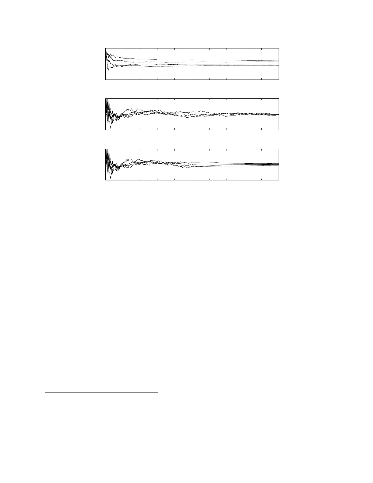
Online Exp ectation-Maximi sation ∗ Olivier Capp ´ e CNRS & T elecom P arisT ec h, Paris, F rance Con ten ts 1 Mo del and Assumptions 3 2 The E M Algorithm and the Limiting EM Recursion 5 2.1 The Batc h EM Algorithm . . . . . . . . . . . . . . . . . . . . . . . . . . . . . . . . 5 2.2 The Limiting EM Recursion . . . . . . . . . . . . . . . . . . . . . . . . . . . . . . . 6 2.3 Limitations of Batc h EM for Long Data Records . . . . . . . . . . . . . . . . . . . 7 3 Online E xp ectation-Maximisation 8 3.1 The Algorithm . . . . . . . . . . . . . . . . . . . . . . . . . . . . . . . . . . . . . . 8 3.2 Con v ergence Pr op erties . . . . . . . . . . . . . . . . . . . . . . . . . . . . . . . . . 9 3.3 Application to Finite Mixtures . . . . . . . . . . . . . . . . . . . . . . . . . . . . . 13 3.4 Use for Batc h Maxim um-Like liho o d Estimation . . . . . . . . . . . . . . . . . . . . 14 4 Discussion 17 Before en tering into any m ore details ab out the metho d ologica l asp ects, let’s discuss the motiv ations b ehind the asso ciation of the tw o phrases “online (estimation)” and “Exp ectatio n- Maximisation (algorithm)” as w ell as their p ertinence in the co nte xt o f mixtures and more general mo dels in vo lving laten t v ariables. The adjectiv e online refers to the idea of compu ting estimates of mo del parameters on-the-fly , without storing the data and b y con tinuously up dating the estimates as more observ ations b ecome a v ailable. In the mac hin e learning literature, the phrase online le arning h as been mostly used re- cen tly to r efer to a sp ecific w a y of analysing th e p erformance of algorithms that incorp orate obser- v ations p r ogressiv ely (C ´ esa-Bianc hi and Lugosi, 2006). W e d ot not refer here to this approac h and will only consider the more traditional setup in whic h the ob jectiv e is to estimate fixed parameters of a statistical mo d el and the p erformance is quantified b y the p ro ximit y b et ween the estimates and the parameter to b e estimated. In signal p ro cessing and con trol, the sort of algorithms con- sidered in the foll o wing is o ften referred to as adaptive or r e cursive (Lj ung and S¨ oderstr¨ om, 198 3 , Ben v eniste et al., 1990 ). The w ord recursive is so ubiquitous in compu ter science that its u se ma y b e s omewh at am biguous and is not recommended. Th e term adaptiv e m a y refer to the t yp e of algorithms co nsid ered in this c h apter b ut is also often used in cont exts where the focus is on the abilit y to trac k slow drifts or abrup t c h an ges in the m o del parameters, wh ich will not b e our primary concerns. ∗ T o app ear in Mixtur es , edited b y Kerrie Mengersen, Mike Titterington and Christian P . Rob ert. 1 T raditional applications of online algorithms in vo lve situations in whic h the data cannot b e stored, due to its v olum e and rate of sampling as in real-t ime signal pro cessing or s tr eam m in ing. The wide av ailabilit y of ve ry large datasets in volving thousands or millions of examples is also at the origin of the curren t renewe d in terest in online algorithms. In this con text, online algo- rithms are ofte n more efficien t —i.e., con v erging faster to wards the ta rget p arameter v alue— and need few er computer resource, in terms of memory or disk access, than their batc h counte rp arts (Neal and Hin ton , 1999). In this c hapter, w e are in terested in b oth con texts: when the online al- gorithm is used to p ro cess on-the-fly a potentia lly un limited amount of data or when it is applied to a fixed but large datase t. W e will r efer to the latter con text as the b atch estimation mod e. Our m ain in terest is maxim um lik eliho o d estimation and although we ma y consider adding a p enalt y term (i.e., Maxim u m A P osteriori estimatio n), w e will not consider “fully Ba yesia n” meth- o ds which aim at sequ entially sim ulating from the parameter p osterior. T h e main motiv ation f or this restriction is to stick to computationally simp le iterat ions whic h is an essen tial requir ement of successful online metho ds. In particular, when online algorithms are used for batc h estimation, it is required that eac h parameter up date can b e carried out v ery efficie ntly for the metho d to b e com- putationally comp etitiv e with traditio nal batc h estimation algorithms. F u lly Ba ye sian approac h es —see, e.g., (Ch opin, 2002)— t ypically require Mon te Carlo sim u lations ev en in simple mod els and raise some c hallenging stabilit y issues when used on v ery long data records (Kan tas et al., 2009). This quest for simplicit y of eac h of the parameter u p date is also the r eason for fo cussing on the EM (Exp ectation-Ma ximisation) algo rithm. Ev er since its in tro duction b y Dempster et al. (1977), th e EM al gorithm has been criticise d for its often sub-optimal conv ergence b eh a viour and man y v ariants ha ve b een p rop osed by , among others, Lange (1995), Meng and V an Dyk (199 7 ). This b eing said, thir t y y ears after the seminal pap er b y Dempster and his coauthors, the EM algorithm still is, b y far, the most widely used inference tool for laten t v ariable mo dels due to its n umerical stabilit y and ea se of implemen tation. Our main p oin t here is not to argue that the EM algorithm is alw ays preferable to other options. But the EM algo rithm whic h do es not rely on fine n umerical tunings in v olving, for instance, line-searc hes, r e-pro jections or pre-conditioning is a p erfect cand id ate for dev eloping online v ersions with very simple up dates. W e hop e to con v in ce the reader in the rest of this chapter that the online version of EM that is describ ed here shares man y of the attractiv e prop erties of the original prop osal of Demps ter et al. (1977) and pro vides an easy to implemen t and robust solution for online estimation in laten t v ariable mo dels. Quite obvio usly , guaran teeing the strict lik eliho o d ascen t pr op ert y of the original EM algorithm is hard ly feasible in an online co ntext. On the other hand, a remark able prop ert y of the onlin e EM algorithm is that it can reac h asymptotic Fisher efficiency b y conv erging tow ards the actual parameter v alue at a rate w hic h is equiv alen t to that of the Maxim um Lik eliho o d Es timator (MLE). Hence, w hen th e num b er of observ ations is sufficien tly large, the online EM alg orithm do es b ecomes h ighly comp etitiv e and it not necessary to consider p oten tially faster-con ve rging alternativ es. When used for batc h estimation, i.e., on a fixed large d ataset, the situation is more con trasted but w e will nonetheless sho w that the online algorithm do es con ve rge tow ards th e maxim um lik eliho o d parameter estimate corresp onding to the whole d ata. T o achiev e this resu lt, one t ypically needs to scan the data set rep eatedly . In terms of computing time, the adv an tages of using an online alg orithm in this situation will t ypically dep en d on the size of the problem. F or long data records how ev er, this approac h is certainly more recommendable than the use of the traditional batc h EM algorithm and preferable to other alternativ es considered in the literature. The r est of this c hapter is organised as follo ws. Th e fir st section is dev oted to the mo delling assumptions that are adopted throughout the c hapter. In Sectio n 2, w e co nsid er the large-sample b ehavio ur of the tr aditional EM algorithm, insisting on the concept of th e limiting EM recursion 2 whic h is instrumental in th e design of the online algorithm. The v arious asp ects of the online EM algorithm are then examined in Sections 3 and 4. Although th e c h ap ter is in tended to b e s elf-con tained, we will nonetheless assu me th at the reader is familiar with the fundamenta l concepts of classical statistical inference and, in p articular, with Fish er in f ormation, exp onent ial families of distributions and maxim um lik eliho o d estimation, at the lev el of Lehmann and Casella (199 8 ), Bic k el and Do ksum (200 0 ) or equiv alen t texts. 1 Mo d el and Assumptions W e assume that w e are able to observe an indep end en t sequence of iden tically distributed d ata ( Y t ) t ≥ 1 , with margi nal distr ibution π . An imp ortan t remark is that w e do not necessarily assume that π corresp onds to a distrib ution that is reac hable b y the statistical mo del that is used to fit the data. As discussed in Sectio n 3.4 b elo w, this distinction is imp ortan t to analyse the use of the online algo rithm for batc h maximum-lik eliho o d estimatio n. The statistical mo dels that w e consider are of the missing-data t yp e, with an unob s erv able random v ariable X t asso ciated to eac h observ ation Y t . The laten t v ariable X t ma y b e con tinuous or v ector-v alued and we w ill not b e restricting ourselv es to finite m ixtu re mo dels. F ollo wing the terminology in tro d uced by Dempster et al. (197 7 ), w e will r efer to the p air ( X t , Y t ) as the c omplete data . The lik eliho o d fu nction f θ ⋆ is th us defined as the marginal f θ ( y t ) = Z p θ ( x t , y t ) dx t , where θ ∈ Θ is the parameter of in terest to b e estimated. If the actual marginal distribu tion of the data b elongs to the family of the mo del d istr ibutions, i.e., if π = f θ ⋆ for some p arameter v alue θ ⋆ , the mo del is s aid to b e wel l-sp e c i fie d ; but, as mentio ned ab o v e, w e dot not restrict ourselve s to this case. In the follo w ing, the statistical m o del ( p θ ) θ ∈ Θ is assumed to v erify the follo wing k ey requirement s. Assumption 1. Mo del ling Assumptions (i) The mo del b elongs to a (curve d) exp onential family p θ ( x t , y t ) = h ( x t , y t ) exp ( h s ( x t , y t ) , ψ ( θ ) i − A ( θ )) , (1) wher e s ( x t , y t ) is a ve ctor of complete-data sufficient stat istics b elonging to a c onvex set S , h· , ·i denotes the dot pr o duct and A is the log-partition fu nction . (ii) The c omplete-data maximum-likeliho o d is explicit, in the sense that the function ¯ θ define d by ¯ θ : S → Θ S 7→ ¯ θ ( S ) = arg max θ ∈ Θ h S, ψ ( θ ) i − A ( θ ) is available in close d-form. Assumption 1 defines the con text wher e the EM algorithm ma y b e used directly (see, in particular, the discussion of Dempster et al., 1977). Note that (1) is not restricted to the sp ecific case of exp onentia l family distributions in c anonic al (or natur al ) parameterisation. The latter corresp ond to the situation wh er e ψ is the identit y function, whic h is particular in that p θ is then 3 log-co nca ve with the complete-data Fisher information matrix I p ( θ ) b eing given by th e Hessia n ∇ 2 θ A ( θ ) of the log- partition f unction. Of course, if ψ is an inv ertib le function, one could use the reparameterisation η = ψ ( θ ) to reco ve r the natural parameterisatio n but it is imp ortan t to recognise that for many mo dels of in terest, ψ is a function that maps lo w-dimensional parameters to higher-dimensional statistics. T o illustrate th is situation, we will use the follo wing simple runn in g example. Example 2 (Probabilistic PCA Mo d el) . Consider the probabilistic P r incipal Comp onen t Analysis (PCA) mo del of Tipping and Bishop (1999). The mo del p ostulates that a d -dimensional observa- tion v e ctor Y t c an b e r epr esente d as Y t = uX t + λ 1 / 2 N t , (2) wher e N t is a c entr e d unit-c ovarianc e d -dimensional multivaria te Gaussian ve ctor, while the la tent variable X t also is such a ve ctor but of much lower-dimension. Henc e , u is a d × r matrix with r ≪ d . Eq. (2) is thus f ul ly e qu i valent to assuming that Y t is a c entr e d d - dimensional Gaussian vari- able with a structur e d c ovarianc e matrix given by Σ( θ ) = uu ′ + λI d , wher e the prime denotes tr ansp osition and I d is the d -dimensional identity matrix. Cle arly, ther e ar e in this mo del many ways to estimate u and λ that do not r ely on the pr ob abilistic mo del of (2 ) ; the standar d P CA b eing pr ob ably the most wel l-known. Tipping and Bishop (1999) discuss sever al r e asons for using the pr ob abilistic appr o ach tha t include the use of priors on the p ar ameters, the ability to de al with missing or c ensor e d c o or dinates of the observations but also the ac c ess to quantitative diagnos- tics b ase d on the likeliho o d that ar e helpful, in p articular, for determining the numb e r of r elevant factors. T o c ast the mo del of (2 ) in the form given by (1) , the c omplete-data mo del   X t . . . Y t   ∼ N       0 . . . 0   ,     I r . . . u ′ . . . . . . . . . . . . . . . . u . . . uu ′ + λI d         must b e r ep ar ameterise d by the pr e cision matrix Σ − 1 ( θ ) , yielding p θ ( x t , y t ) = (2 π ) − d/ 2 exp  trace  Σ − 1 ( θ ) s ( x t , y t )  − 1 2 log | Σ( θ ) |  , wher e s ( x t , y t ) is the r ank one matrix s ( x t , y t ) = − 1 2   X t . . . Y t     X t . . . Y t   ′ . Henc e i n the pr ob abilistic PCA mo del, the ψ function in this c ase maps the p air ( u, λ ) to the ( d + 1) - dimensional symmetric p ositive definite matrix Σ − 1 ( θ ) . Y e t, Assu mption 1-(ii) holds in this c ase and the EM algorithm c an b e u se d —se e the gener al formulas given in (Tipping and Bishop, 1999) as wel l as the details of the p articular c ase wher e r = 1 b elow. In the fol lowing, we wil l mor e sp e ci fic al ly lo ok at the p articular c ase wher e r = 1 and u is thus a d -dimensiona l ve ctor. This very si mple c ase also pr ovides a nic e and c oncise il lustr ation of mor e c omplex situations, suc h as the Direction O f Arriv al (DO A) mo del c onsider e d by Capp ´ e et al. 4 (2006). The c ase of of a single factor PCA is also inter esting as most r e qu i r e d c alculations c an b e done explicitly. In p articular, it is p ossible to pr ovide the fol lowing expr ession for Σ − 1 ( θ ) using the b lo c k matrix i nv e rsion and Sherman-Morrison formulas: Σ − 1 ( θ ) =     1 + k u k 2 /λ . . . − u ′ /λ . . . . . . . . . . . . . . . . . . . . . . − u/λ . . . λ − 1 I d     . The ab ove expr ession shows that one may r e define the sufficient statistics s ( x t , y t ) as c onsisting solely of the sc alars s (0) ( y t ) = k y t k 2 , s (2) ( x t ) = x 2 t and of the d -dimensional ve ctor s (1) ( x t , y t ) = x t y t . The c omplete-data lo g - likeliho o d is then given by log p θ ( x t , y t ) = C st − 1 2 ( nd log λ + s (0) ( y t ) − 2 u ′ s (1) ( x t , y t ) + s (2) ( x t ) k u k 2 λ ) , (3) ignoring c onstant terms that do not dep e nd on the p ar ameters u and λ . Note that developing an online algo rithm for (2) in this p articular c ase i s e quiv alent to r e- cursively estimating the lar gest eigenvalue of a c ovarianc e matrix fr om a series of multivariate Gaussian observations. We r eturn to this example shortly b elow. 2 The EM Algorithm and the Limiting EM Recursion In this section, w e fir st r eview core elemen ts regarding the EM algorithm that will b e needed in the follo win g. Next, w e in tro d uce the key concept of the limiting EM r e cursion wh ic h corresp onds to the limit ing determin istic iterativ e algorithm obtained when the n umb er of observ ations gro ws to infinity . This limiting EM recursion is imp ortan t b oth to und erstand the b eha viour of classic b atc h EM when used with man y observ ations and for motiv ating the form of the online EM algorithm. 2.1 The Batch EM Algor ithm In ligh t of Assumption 1 and in p articular of the assumed form of the like liho o d in (1), the classic EM algo rithm of Dempster et al. (1977) tak es the follo wing form. Algorithm 3 (Batc h EM Algorithm) . Given n observations, Y 1 , . . . , Y n and an initial p ar ameter guess θ 0 , do, for k ≥ 1 , E-Step S n,k = 1 n n X t =1 E θ k − 1 [ s ( X t , Y t ) | Y t ] , (4) M-Step θ k = ¯ θ ( S n,k ) . ( 5) Returning to the single factor PCA mo d el of Example 2, it is easy to c hec k from the expression of the co mplete-data log-lik eliho o d in (3) and the definition of the sufficien t statistic s that the E- 5 step reduces to the computation of s (0) ( Y t ) = k Y t k 2 , E θ h s (1) ( X t , Y t )    Y t i = Y t Y ′ t u λ + k u k 2 , E θ h s (2) ( X t )    Y t i = λ λ + k u k 2 + ( Y ′ t u ) 2 ( λ + k u k 2 ) 2 , (6) with the corresp onding empirical a v erages S (0) n,k = 1 n n X t =1 s (0) ( Y t ) , S (1) n,k = 1 n n X t =1 E θ k − 1 h s (1) ( X t , Y t )    Y t i , S (2) n,k = 1 n n X t =1 E θ k − 1 h s (2) ( X t )    Y t i . The M-step equations whic h define the function ¯ θ are giv en b y u k = ¯ θ ( u ) ( S n,k ) = S (1) n,k /S (2) n,k , λ k = ¯ θ ( λ ) ( S n,k ) = 1 d n S (0) n,k − k S (1) n,k k 2 /S (2) n,k o . (7) 2.2 The Limiting EM Recursion Returning to th e general ca se, a v ery important remark is th at Algorithm 3 can b e fully reparam- eterised in the domain of sufficien t statistics, redu cing to the recursion S n,k = 1 n n X t =1 E ¯ θ ( S n,k − 1 ) [ s ( X t , Y t ) | Y t ] with th e con ven tion that S n, 0 is suc h that θ 0 = ¯ θ ( S n, 0 ). Clearly , if an uniform (wrt. S ∈ S ) la w of large num b ers holds for the empir ical a v erages of E ¯ θ ( S ) [ s ( X t , Y t ) | Y t ], the EM u p date te nd s, as the n umber of observ ations n tends to infin it y , to the deterministic mapping T S on S defined by T S ( S ) = E π  E ¯ θ ( S ) [ s ( X 1 , Y 1 ) | Y 1 ]  . (8) Hence, the sequence of EM iterates ( S n,k ) k ≥ 1 con v erges to the sequence ( T k S ( S 0 )) k ≥ 1 , whic h is deterministic except f or the c hoice of S 0 . W e refer to the limiting mapping T S defined in (8), as the limiting EM r e cursion . Of course, this mapp in g on S also in duces a mappin g T Θ on Θ by considering the v alues of θ associated to v alues of S b y the function ¯ θ . This second mappin g is defined as T Θ ( θ ) = ¯ θ { E π (E θ [ s ( X 1 , Y 1 ) | Y 1 ]) } . (9) Using exactly the same argumen ts as those of Dempster et al. (1977 ) for the classic EM algorithm, it is straigh tforward to c hec k that u n der suitable regularit y assumptions, T Θ is suc h that 6 1. Th e Kullbac k-Leibler diverge nce D ( π | f θ ) = R log π ( x ) f θ ( x ) π ( x )d x is a Lyapuno v function for the mapping T Θ , that is, D  π | f T Θ ( θ )  ≤ D ( π | f θ ) . 2. Th e set of fixed p oin ts of T Θ , i.e., suc h that T Θ ( θ ) = θ , is giv en b y { θ : ∇ θ D ( π | f θ ) = 0 } , where ∇ θ denotes the gradien t. Ob viously , (9) is not directly exploitable in a statist ical con text as it in v olv es integ rating und er the un kno wn distribution of the observ ations. Th is limiting EM recursion can ho w ev er b e used in the con text of adaptive Monte Carlo metho ds (Capp´ e et al., 2008) and is known in mac h in e learning as part of the informa tion b ottlene ck framework (Slonim and W eiss, 2003). 2.3 Limitations of Batch E M for Long Data R ecords But the main interest of (9) is to pro vide a clear understandin g of the b eha viour of the EM algo- rithm when used w ith very long data records, justifying muc h of th e in tuition of Neal and Hinton (1999). Note that a large part of the p ost 1980’s literature on the EM algo rithm focu s ses on accele rating conv ergence to wards the MLE for a fixed data size. Here, w e consider the related but v ery differen t issue of understand ing the b eha viour of the EM algorithm when the data size increases. Figure 1 displa ys the r esults obtained with the batc h EM algorithm for the single comp onen t PCA mo del estimated from data sim ulated u nder the mo d el w ith u b eing a 20-dimensional v ector of unit norm and λ = 5. Both u and λ are treated as unkno w n parameters bu t only the e stimated squared norm of u is displa ye d on Figure 1, as a fun ction of the num b er of EM iterations and for t wo differen t data sizes. Note that in this ve ry simple mo del, the observ ation lik eliho o d b eing giv en the N (0 , uu ′ + λI d ) densit y , it is straigh tforward to c hec k th at the Fisher information for the parameter k u k 2 equals { 2( λ + k u k 2 ) 2 } − 1 , w h ic h has b een used to represent the asymptotic confidence int erv al in grey . The width of this in terv al is m eant to b e directly comparable to that of the whisk ers in the b o x-and-whisker plots. Bo xplots are u s ed to su m marise the results obtained from one thousand indep end en t runs of the method . Comparing the top and b ottom plots clearly sho w s that wh en the n umb er of iteratio ns in- creases, the tra jectories of the EM al gorithm con verge to a fixed deterministic tra jectory whic h is that of the limiting EM r ecur sion ( T k Θ ( θ 0 )) k ≥ 1 . Of course, this tra jectory dep ends on the c h oice of the initial p oin t θ 0 whic h w as fixed throughout this exp eriment . It is also observ ed that the monotone increase in the lik eliho o d guaran teed b y the EM algo rithm do es not necessarily imply a monotone con v ergence of all parameters to wards the MLE. Hence, if the num b er of EM iterations is k ept fixed, the estimates returned b y the batc h EM alg orithm with the la rger num b er o f obser- v ations (b ottom p lot) are not significan tly imp r o v ed desp ite the ten-fold increase in computation time (the E step computations m ust b e done f or all observ ations and h ence th e complexit y of the E-step scales prop ortionally to th e num b er n of observ ations). F rom a statistic al p ersp ectiv e, the situation is e ven less satisfying a s estimation errors that were not statistically significan t for 2,00 0 observ ations can b ecome significan t when the n umb er of obs er v ations increases. In the upp er plot, in terruptin g th e EM al gorithm after 3 or 4 iterations do es pro d uce estimates that are statistically acceptable (comparable to the exact MLE) b ut in the lo wer p lot, ab out 20 iterations are n eeded to ac h iev e the desired precision. As suggested by Neal and Hinto n (1999), this parado xical situation can to some exten t b e a voided b y up dating the parameter (that is, applying the M-step) more often, without w aiting for a complete scan of the data record. 7 0 1 2 3 4 1 2 3 4 5 6 7 8 9 10 11 12 13 14 15 16 17 18 19 20 Batch EM iterations ||u|| 2 20 10 3 observations 0 1 2 3 4 1 2 3 4 5 6 7 8 9 10 11 12 13 14 15 16 17 18 19 20 ||u|| 2 2 10 3 observations Figure 1: Conv ergence of batc h EM estimates of k u k 2 as a fu nction of the n umb er of EM iterations for 2,00 0 (top) and 20,0 00 (b ottom) observ ations. The b o x-and-whisker plots (outliers plotting suppr essed) are computed from 1,00 0 ind ep end ent replicatio ns of the sim ulated data. The grey region corresp onds to ± 2 in terquartile range (appro x. 99 . 3% co v erage) under the asymptotic Gaussian appro ximation of the MLE. 3 Online Exp ectation-Maximisation 3.1 The Algorithm The limiting-EM argumen t dev elop ed in the follo w ing section sh o ws that when the num b er of observ ations tends to infinit y , the EM algorithm is tryin g to lo cate the fixed p oints of the mappin g T S defined in (8), that is, the ro ots of the equation E π  E ¯ θ ( S ) [ s ( X 1 , Y 1 ) | Y 1 ]  − S = 0 . (10) Although w e cannot compute the required exp ectation wrt. the un kno wn distribution π of the data, eac h new observ ation pro vides u s with an unbiased noisy observ ation of th is quantit y through E ¯ θ ( S ) [ s ( X n , Y n ) | Y n ]. Solving (10) is th u s an instance of the most basic case where the Stoc hastic Appro ximation (or Robb ins-Monro) metho d can b e used. Th e literature on Sto chastic App ro x- imation is h uge b ut we recommend the textb o oks b y Ben v eniste et al. (1990), Ku shner and Yin (2003) for more details and examples as w ell as the review pap er by Lai (2003) for a historical p ersp ectiv e. Th e standard s to c hastic approximat ion app r oac h to appr o ximate the solution of (10) is to compute S n = S n − 1 + γ n  E ¯ θ ( S n − 1 ) [ s ( X n , Y n ) | Y n ] − S n − 1  , (11) for n ≥ 1, S 0 b eing arbitrary and ( γ n ) n ≥ 1 denoting a sequence of p ositiv e stepsizes that decrease to zero. This equation, rewritten in an equiv alen t form b elo w, is the mai n in gredien t of the online 8 EM algo rithm. Algorithm 4 (Online EM Algorithm) . Given S 0 , θ 0 and a se q uenc e of stepsizes ( γ n ) n ≥ 1 , do, for n ≥ 1 , Sto c hastic E-Step S n = (1 − γ n ) S n − 1 + γ n E θ n − 1 [ s ( X n , Y n ) | Y n ] , (12) M-Step θ n = ¯ θ ( S n ) . (13) Rewriting (10) un der the form displa y ed in (12) is v ery enligh tening as it sh o ws that the n ew statistic S n is obtained as a con ve x com bination of the pr evious statistic S n − 1 and of an u p d ate that dep end s on the new observ ation Y n . In particular it sh o ws that the stepsizes γ n ha v e a natural scale as their highest a dmiss ible v alue is equal to one. This means th at one can safely take γ 1 = 1 and that only the rate at whic h th e stepsize decreases n eeds to b e selected carefully (see b elo w). It is also observ ed that if γ 1 is set to one, the initial v alue of S 0 is nev er used and it suffices to select the initial p ar ameter guess θ 0 ; this is the approac h used in the follo wing s imulations. The only adju stmen t to Alg orithm 4 that is n ecessary in p ractice is to o mit the M-step of (13) for the first observ ations. It typica lly ta ke s a few observ ations b efore the complete-data maximum lik eliho o d solution is well -defin ed and the parameter up date s h ould b e inh ibited during this early phase of training (Capp ´ e and Moulines, 2009). In the sim ulations presen ted b elo w in Sectio ns 3.2 and 3.4, the M-step w as omitt ed for the first fiv e obs er v ations o nly but in m ost complex scenarios a longer initial parameter freezing phase ma y b e necessary . When γ 1 < 1, it is tempting to in terp ret the v alue of S 0 as b eing asso ciated to a prior on the parameters. Indeed, the c hoice of a c onju gate prior for θ in the exp onen tial family defined b y (1) do es result in a complete-data Maxim um A P osteriori (MAP) estimate of ¯ θ giv en b y ¯ θ ( S n,k + S 0 /n ) (instead of ¯ θ ( S n,k ) for the MLE), w h ere S 0 is the h yp er-parameter of the prior (Rober t, 2001). Ho wev er, it is easily c heck ed that the in fluence of S 0 in S n decreases as Q n k =1 (1 − γ k ), w hic h for the suitable stepsize decrease sc hemes (see b eginning of S ection 3.2 b elo w), d ecreases faster than 1 /n . Hence, the v alue of S 0 has a rather limited impact on the con v ergence of the onlin e EM algorithm. T o ac hieve MAP estimation (assumin g a conjugate pr ior on θ ) it is thus recommend to replace (13) b y θ n = ¯ θ ( S n + S 0 /n ), where S 0 is the h yp erparameter of the prior on θ . A last remark of imp ortance is that Algorithm 4 can most naturally b e interpreted as a sto c hastic approximat ion r ecursion on the s u fficien t statistics r ather than on the parameters. T h ere do es not exists a similar algorithm that op erates directly on the parameters b ecause un biased appro ximations of the rhs. of (9) based on the observ ations Y t are n ot easily a v ailable. As w e will see b elo w, Algo rithm 4 is asymptotically equiv alen t to a gradien t recursion on θ n that inv olves an additional matrix w eigh ting w hic h is not necessary in (12). 3.2 Con v ergence Prop erties Under the assu m ption that the stepsize sequence s atisfies P n γ n = ∞ , P n γ 2 n < ∞ and other reg- ularit y h yp otheses that are omitte d here (see Capp´ e and Moulines , 200 9 for detai ls) the follo wing prop erties c haracterise the asymp totic b eha viour of the online EM algorithm. (i) Th e estimate s θ n con v erge to the set of ro ots of the equation ∇ θ D ( π | f θ ) = 0. 9 (ii) The algo rithm is asymptotically equiv alen t to a gradient al gorithm θ n = θ n − 1 + γ n J − 1 ( θ n − 1 ) ∇ θ log f θ n − 1 ( Y n ) , (14) where J ( θ ) = − E π  E θ  ∇ 2 θ log p θ ( X 1 , Y 1 )   Y 1  . (iii) F or a w ell sp ecified mo d el (i.e., if π = f θ ⋆ ) and u nder Polyak-Rup p ert aver aging , θ n is Fisher efficien t: sequences that do con v erge to θ ⋆ are suc h that √ n ( θ n − θ ⋆ ) con verges in distribution to a cen tred multiv ariate Gaussian v ariable with cov ariance matrix I π ( θ ⋆ ), wher e I π ( θ ) = − E π [ ∇ 2 θ log f θ ( Y 1 )] is the Fisher information matrix corresp onding to the observe d data. P oly ak-Rupp ert a veraging refers to a p ostpro cessing step whic h simply consists in r eplacing the estimate d parameter v alues θ n pro du ced b y the algorithm by their a ve rage ˜ θ n = 1 n − n 0 n X t = n 0 +1 θ n , where n 0 is a p ositive in dex at which a ve raging is started (P oly ak and Juditsky, 1992, Rupp ert, 1988). Regarding the state ments (i) and (ii) ab o v e, it is imp ortan t to understand that the limiting estimating equation ∇ θ D ( π | f θ ) = 0 ma y hav e m ultiple solutions, ev en in well- sp ecified mo dels. In practice, the most imp ortan t factor that influences the conv ergence to one of the stationary p oin ts of the Ku llbac k-Leibler dive rgence D ( π | f θ ) rather th an the other is the c hoice of the initial v alue θ 0 . An additional imp ortant remark ab out (i)–(iii) is the f act that the asymptotic equiv alent gradien t algorithm in (14) is not a practical algorithm as the matrix J ( θ ) dep ends on π and h ence cannot b e computed. Note also that J ( θ ) is (in general) neither equal to the complete-data information matrix I p ( θ ) nor to th e actual Fisher information in the obs er ved mo del I π ( θ ). The form of J ( θ ) as wel l as its role to a pp ro ximate th e conv ergence b ehavio ur of the EM algorithm follo ws the idea of Lange (199 5 ). F rom our exp erience, it is generally sufficien t to consider stepsize sequences of th e form γ n = 1 /n α where the useful range of v alues for α is from 0.6 to 0.9. The most robust setting is obtained when taking α close to 0 . 5 and using Poly ak-Rupp ert a ve raging. The latter ho wev er requires to c hose an index n 0 that is sufficient ly large and , hence, some idea of the con v ergence time is necessary . T o illustrate these observ ations, Figure 2 displa ys th e results of online EM estimation for the s ingle comp onen t PCA mo del, exactly in the same conditions as those considered previously for batc h EM estimati on in Section 2.3. F rom a computational p oint of view, the main differen ce b etw een the online EM algorithm and the batc h EM algorithm of S ection 2.1 is that the online algorithm p erforms the M-step up date in (7) after eac h observ ation, according to (13), wh ile the batc h E M algorithm only app lies the M-step up d ate after a complete scan of all a v ailable observ ations. Both algorithms ho w ev er require the computatio n of the E-step statistics follo wing (6) for eac h observ ation. In batc h EM, these lo cal E-step computation are acc umulated, follo wing (4), while the online algorithm recursiv ely a v erages these according to (12). Hence, as the computational complexit y of the E and M steps are, in this case, comparable, the compu tational complexit y of the online estimation is equiv alen t to that of one or t wo b atc h EM iterat ions. With this in mind, it is ob vious that the results of Figure 2 compare v er y fa vo urably to those of Figure 1 w ith an estimati on p erformance that is compatible with th e s tatistica l uncertain t y for observ ation lengths of 2,000 and larger (last tw o b o xplots on the righ t in eac h displa y). 10 0 1 2 3 4 0.2 10^3 2 10^3 20 10^3 Number of observations ||u|| 2 α = 0.6 with halfway averaging 0 1 2 3 4 0.2 10^3 2 10^3 20 10^3 ||u|| 2 α = 0.6 0 1 2 3 4 0.2 10^3 2 10^3 20 10^3 ||u|| 2 α = 0.9 Figure 2 : Online EM estimates of k u k 2 for v arious data sizes (2 00, 2,000 and 20,00 0 observ ations, from left to righ t) and algorithm settings ( α = 0 . 9, α = 0 . 6 and α = 0 . 6 with Poly ak-Rupp ert a v eraging, fr om top to b ottom). The b ox- and-wh isk er plots (outliers plotting su p pressed) are computed fr om 1,000 ind ep endent replications of the simulate d data. The grey regions corresp onds to ± 2 in terqu artile r ange (approx. 99 . 3% co ve rage) un der the asymp totic Gaussian appro ximation of the MLE. Regarding the choic e of the stepsize d ecrease exp onen t α , it is observ ed that while the c hoice of α = 0 . 6 (midd le plot) d o es resu lt in m ore v ariability than the c hoice of α = 0 . 9 (top p lot), esp ecially for smaller observ ation sizes, the long-run p erformance is somewhat b etter with the former. In particular, when P olya k-Rup p ert a veragi ng is used (b ottom plot), the p er f ormance for the longest data size (20,00 0 observ ations) is clea rly compatible with the claim that online EM is Fisher-efficien t in this case. A practical concern asso ciated with a v eraging is the c hoice of the initial instant n 0 where av eraging starts. In the case of Figure 2, we c ho ose n 0 to b e equal to half the length of eac h data record, h ence a verag ing is used only on the second half of the data. While it pro duces refined estimate s for the longer data sizes, one can observe that the p erformance is rather degraded for th e smallest observ ation size (200 observ ations) due to the fact that the algorithm is still very far from ha vin g conv erged after just 100 observ ations. Hence, a v eraging is efficien t b ut d o es r equire to c h ose a v alue of n 0 that is sufficien tly la rge so as to a vo id in tro du cing a bias due to the lac k of con verge nce. In our exp erience, the f act that c hoices of α close to 0.5 are more r eliable than v alues closer to the u pp er limit of 1 is a very constant obs er v ation. It ma y come to some surpr ise for readers familiar with th e gradien t d escen t algorithm as used in numerical optimisation, whic h shares some similarit y with (12). In this case , it is kno wn that the optimal stepsize choic e is of the form γ n = a ( n + b ) − 1 for a br oad cla ss of functions (Nestero v , 2003). Ho w ev er, the situation h ere is very different as w e do not observe exact gradien t or exp ectations but only noisy v ersion of 11 0 200 400 600 800 1000 1200 1400 1600 1800 2000 −2 0 2 u 1 Number of observations α = 0.6 with halfway averaging 0 200 400 600 800 1000 1200 1400 1600 1800 2000 −2 0 2 u 1 α = 0.6 0 200 400 600 800 1000 1200 1400 1600 1800 2000 −2 0 2 u 1 α = 0.9 Figure 3: F our sup erimp osed tra jectories of the estimate of u 1 (first comp onent of u ) for v arious algorithm settings ( α = 0 . 9, α = 0 . 6 and α = 0 . 6 w ith P olya k-Rupp ert a v eraging, from top to b ottom). The actual v alue of u 1 is equal to zero. them 1 . Figure 3 shows that while th e tra jectory of the p arameter estimate s app ears to b e muc h rougher and v ariable with α = 0 . 6 than with α = 0 . 9, the bias caused by the initialisation is also forgotten m uch more rapidly . It is also observed that the use of a v eraging (bottom d ispla y) mak es it p ossible to ac hiev e the b est of b oth w orld s (rapid forgetting of the initia l condition and smo oth tra jectories). Liang and Klein (2009) considered the p erformance of the online EM algorithm for large- scale natural language pro cessing ap p lications. This domain of application is charac terised by the use of v ery large-dimensional m o dels, most often related to the multinomial distribu tion, in v olving tens of thousands of differen t w ords and tens to hundreds of seman tic tags. As a consequence, eac h obs er v ation, b e it a sent ence or a whole do cumen t, is p o orly informativ e ab ou t the mo del parameters (typica lly a giv en text con tains only a v ery limited p ortion of the whole av ailable v o cabulary). In this con text, Liang and Klein (2009) found that the algorithm w as highly com- p etitiv e with other approac hes but only wh en com bined with mini-b atch blo cking : rather than applying Algorithm 4 at the observ ation sca le, the algorithm is u sed on min i-batc h es consisting of m consecutiv e observ ations ( Y m ( k − 1)+1 , Y mk +2 . . . , Y mk ) k ≥ 1 . F or the mo dels and data considered b y Liang and Klein (2009), v alues of m of up to a few thousands yielded optimal p erformance. More generally , mini-batc h blo c king can b e useful in dealing with mixture-lik e mo dels with rarely activ e comp onen ts. 1 F or a complete-data exp onential family mo d el in natural parameteris ation, it is easily chec ked th at E θ [ s ( X n , Y n ) | Y n ] = E θ [ s ( X n , Y n )] + ∇ θ log f θ ( Y n ) and hen ce that the recursion in the space of sufficient statis- tics is indeed very close to a gradien t as cent algorithm. H o wev er, w e only have access to ∇ θ log f θ ( Y n ) which is a noisy v ersion of th e gradient of th e actual limiting ob jective function D ( π | f θ ) that is minimised. 12 3.3 Application to Finite Mixtures Although we considered so far only the simple case of Example 2 whic h allo ws for the compu- tation of the Fisher information matrix and h ence f or quan titativ e assessmen t of the asymptotic p erforman ce, the online EM algorithm is easy to imp lement in mo dels in vo lving finite mixture of distributions. Figure 4 disp la y s the Ba yesian net work representa tion corresp ondin g to a mixtu re mo del: for eac h ob s erv ation Y t there is an unobserv able mixture indicator or allocation v ariable X t that tak es its v alue in the set { 1 , . . . , m } . A t ypical parameterisation for this mo d el is to hav e a separate sets of parameters ω and β for, resp ectiv ely , the parameters of the prior on X t and of the conditional distribu tion of Y t giv en X t . Usually , ω = ( ω (1) , . . . , ω ( m ) ) is c hosen to b e the collectio n of comp onent frequ en cies, ω ( i ) = P θ ( X t = i ), and hence ω is constrained to the p robabilit y simplex ( ω ( i ) ≥ 0 and P m i =1 ω ( i ) = 1). The observ ation p df is most often parameterised as f θ ( y t ) = m X i =1 ω ( i ) g β ( i ) ( y t ) , where ( g λ ) λ ∈ Λ is a p arametric family of probab ility densities and β = ( β (1) , . . . , β ( m ) ) are the comp onent -sp ecific p arameters. W e assume that g λ ( y t ) has an exp onen tial family r ep resen tation similar to that of (1) with sufficien t statistic s ( y t ) and maxim u m lik eliho o d function ¯ λ : S 7→ Λ, whic h is suc h that ¯ λ ( 1 n P n t =1 s ( Y t )) = arg max λ ∈ Λ 1 n P n t =1 log g λ ( Y t ). It is th en ea sily chec k ed that the complete- data lik eliho o d p θ b elongs to an exp onentia l family w ith su fficien t statistics s ( ω, i ) ( X t ) = 1 { X t = i } , s ( β ,i ) ( X t , Y t ) = 1 { X t = i } s ( Y t ) , for i = 1 , . . . , m . And the function ¯ θ ( S ) can then b e decomp osed as ω ( i ) = S ( ω, i ) , β ( i ) = ¯ λ  S ( λ,i ) /S ( ω, i )  , fo r i = 1 , . . . , m . . Hence the online EM algorithm tak es the follo wing sp ecific form. Algorithm 5 (Online EM Algorithm for Finite Mixtures) . Given S 0 , θ 0 and a se quenc e of stepsizes ( γ n ) n ≥ 1 , do, for n ≥ 1 , Sto c hastic E-Step Compute P θ n − 1 ( X t = i | Y t ) = ω ( i ) n − 1 g β ( i ) n − 1 ( Y t ) P m j =1 ω ( j ) n − 1 g β ( j ) n − 1 ( Y t ) , and S ( ω, i ) n = (1 − γ n ) S ( ω, i ) n − 1 + γ n P θ n − 1 ( X t = i | Y t ) , S ( β ,i ) n = (1 − γ n ) S ( β ,i ) n − 1 + γ n s ( Y t ) P θ n − 1 ( X t = i | Y t ) , (15) for i = 1 , . . . , m . 13 Y t X t ω β t ≥ 1 Figure 4: Ba yesian net w ork r ep resen tation of a mixture mo del. M-Step ω ( i ) n = S ( ω, i ) n , β ( i ) n = ¯ λ  S ( λ,i ) n /S ( ω, i ) n  . (16) Example 6 (Onlin e EM for Mixtures of P oisson) . W e c onsider a simplistic i nstanc e of Algorithm 5 c orr esp onding to the mixtur e of Poisson distr ibution (se e also Se ction 2.4 of Capp ´ e and Moulines, 2009). In the c ase of th e Poisson distribution, g λ ( y t ) = 1 y t ! e − λ λ y t , the sufficie nt statistic r e duc es to s ( y t ) = y t and the MLE function ¯ λ also is the identity ¯ λ ( S ) = S . Henc e, the online EM r e cursion for this c ase simply c onsists in i nstantiating (15) – (16) as S ( ω, i ) n = (1 − γ n ) S ( ω, i ) n − 1 + γ n P θ n − 1 ( X t = i | Y t ) , S ( β ,i ) n = (1 − γ n ) S ( β ,i ) n − 1 + γ n Y t P θ n − 1 ( X t = i | Y t ) , and ω ( i ) n = S ( ω, i ) n , β ( i ) n = S ( λ,i ) n /S ( ω, i ) n . 3.4 Use for Batch Maxim um-Lik eliho o d Estimation An interesti ng issue that deserv es some more comment s is th e use of the online EM algorithm for batc h estimation from a fixed data record Y 1 , . . . , Y N . In this case, the ob jectiv e is to sa ve on computational effort compared to the use of the batc h EM algorithm. The analysis of the con v ergence b eha viour of online EM in this con text is made easy b y the follo win g observ ation: Prop erties (i ) and (ii ) stated at the b eginning of Section 3.2 do not rely on the assum p tion that the mo del is well- sp ecified (i.e., that π = f θ ⋆ ) and can th us b e app lied with 14 π b eing th e empirical distribution ˆ π N ( dy ) = 1 N P N t =1 δ Y t ( dy ) asso ciated to the observe d sample 2 . Hence, if th e online EM algorithm is app lied by randomly d ra wing (with r eplacemen t) subsequent “pseudo-observ ations” from the fin ite set { Y 1 , . . . , Y N } , it con ve rges to p oints su c h that ∇ θ D ( ˆ π N | f θ ) = − 1 N ∇ θ N X t =1 log f θ ( Y t ) = 0 , that is, stationary p oint s of the log-l ike liho o d of the observ ations Y 1 , . . . , Y N . Prop erty (ii) also pro vides an asymptotic equiv alen t of the online EM u p d ate, wh er e the index n in (14) should b e understo o d as the num b er of online EM steps rather than the num b er of actual observ ation, whic h is here fixed to N . In practice, it d o esn’t app ear that dra wing r andomly the pseudo-observ ations make an y r eal difference when the observ ations Y 1 , . . . , Y N are themselv es already indep endent, except for v ery short data r ecords. H ence, it is more co nv enient to scan the observ ation systematically in tours of length N in w hic h eac h observ ation is visited in a predetermined order. A t th e end of eac h tour, k = n/ N is equal to the num b er of batc h tours completed since the start of the online EM algorithm. T o compare the n umerical efficiency of this approac h with that of th e usual batc h EM it is in teresting to bring together tw o r esults. F or online EM, based o n (14 ), it is p ossible to s ho w that √ n ( θ n − θ ∞ ) con verge s in distribu tion t o a m ultiv ariate Gaussian distribution, where θ ∞ denotes the limit of θ n 3 . In con tr ast, the batc h EM algorithm ac hiev es so-cal led linear con ve rgence whic h means that for suffi cien tly large k ’s, there exists ρ < 1 suc h that k θ k − θ ∞ k ≤ ρ k , where θ k denotes the p arameter estimate d after k batc h EM iterations (Dempster et al., 1977, Lange, 1995). In terms of compu ting effort, the num b er k of batc h EM iterations is comparable to the num b er k = n/ N of batc h tours in the online EM algorithm. Hence the previous theoretical results suggest that • If the num b er of a v ailable observ ations N is sm all, batc h EM can b e w a y faster than the online EM algorithm, esp ecially if one w an ts to obtain a v er y accurate numerical app r o ximation of the MLE. Note that from a statistical viewp oin t, this ma y b e un necessary as the MLE itself is o nly a pro xy for the actual parameter v alue, with an error th at is o f order 1 / √ N in regular statistical mo dels. • When N increases, the onlin e EM algorithm b ecomes p referable and, indeed, arbitrary so if N is sufficient large. Recall in particular from S ection 3.2 that w hen N increases, the online EM estimate obtained after a single b atch tour is asymptotically equiv alen t to the MLE whereas the estimate obtained after a single batc h EM iteratio n con ve rges to the deterministic limit T Θ ( θ 0 ). In their pioneering work on this topic, Neal and Hin ton (1999) suggested an algorithm called incr emental EM as an alternativ e to the batc h EM algorithm. The incremen tal EM algorithm turns out to b e exactl y equiv alent to Algo rithm 4 used with γ n = 1 /n u p to the end of the batc h tour only . After this initial b atch scan, the incremental EM pro ceeds a bit differen tly b y replacing one b y one the pr eviously co mpu ted v alues of E θ t − 1 [ s ( X t , Y t ) | Y t ] with E θ t − 1 +( k − 1) N [ s ( X t , Y t ) | Y t ] when pro cessing the observ ation at p osition t f or the k -th time. This in cremen tal EM algorithm is indeed more efficient than b atc h EM, although they do not necessarily hav e the same complexit y — a p oin t that will b e fu rther d iscu ssed in the next section. F or large v alues of N ho w ev er, incremental 2 Where δ u ( dy ) denotes the Dirac measure localised in u . 3 Strictly speaking, this has been show n only for random b atc h scans. 15 EM b ecomes imp ractical (d ue to the use of a storag e space that increases prop ortionally to N ) and less r ecommendable than the online EM alg orithm as shown by the follo wing example (see also the exp eriments of Liang and Klein, 2009 for similar conclusions). −1.58 −1.56 −1.54 1 2 3 4 5 batch tours Online EM −1.58 −1.56 −1.54 1 2 3 4 5 Incremental EM −1.58 −1.56 −1.54 1 2 3 4 5 Batch EM Figure 5: Normalised log-lik eliho o d of the estimates obtained with, fr om top to b ottom, batc h EM, incrementa l EM and online EM as a function of the n umb er of batc h tours (or iterat ions, for batc h E M). T h e data is of length N = 100 and the b o x an whisk ers plots summarise th e results of 500 indep endent ru ns of the alg orithms started from randomised starting p oints θ 0 . Figure 5 d ispla ys the normalised log -lik eliho o d v alues corresp onding to the th ree estimation algorithms (batc h EM, incremen tal EM and online EM) u sed to estimate the parameters of a mixture of t wo P oisson distribu tions (see Example 6 for implemen tation details) 4 . All data is sim ulated from a mixture mo del with p arameters ω (1) = 0 . 8, β (1) = 1 and β (2) = 3. In this setting, where the sample size is fixed, it is more difficult to come up with a faithfu l illustration of the merits o f eac h approac h as the con vergence b eha viour of the alg orithms d ep end v er y muc h on the data record and o n the initialisation. In Figures 5 and 6 , the t wo data sets w ere kept fixed throughout the simulations but the initiali sation of b oth Po isson means w as rand omly c hosen from the interv al [0.5,5]. This rand omisation a v oids fo cussing on particular algorithm tra jectories and giv es a goo d idea of the general situation, although some v ariations can still b e observ ed when v arying the observ ation records. Figure 5 corresp onds to the case of an observ ation sequence of length N = 100. In this case it is observ ed that the p erformance of incremen tal EM dominates that of the other tw o algorithms, while the online EM alg orithm only b ecomes preferable to batc h EM afte r the second b atc h tour. F or the data record of length N = 1,000 (Figure 6), online EM no w dominates the other tw o 4 Obviously , the fact t hat only log-likelihoo ds normalised by the length of the data are p lotted hides some imp or- tant asp ects of th e prob lem, in particular the lac k of iden tifiability caused b y t he u nknown lab elling of th e mixtu re compon ents. 16 −1.6 −1.58 −1.56 1 2 3 4 5 batch tours Online EM −1.6 −1.58 −1.56 1 2 3 4 5 Incremental EM −1.6 −1.58 −1.56 1 2 3 4 5 Batch EM Figure 6: Same display as in Figure 5 for a data record of length N = 1,000. algorithms, with incremen tal still b eing pr eferab le to batc h EM. Notice that it is also th e case after th e first b atc h tour, illustrating our claim that the c hoice of γ n = n − 0 . 6 used here for the online EM algorithm is ind eed pr eferab le to the v alue of γ n = n − 1 , wh ic h coincides with the u p date used b y the incremen tal EM algorithm during the first b atc h tour. Finally , one can observ e on Figure 6 t hat eve n after fiv e EM iterations there are a few starting v alues for whic h b atc h EM or incremen tal EM gets stuck in regions of lo w normalised log-lik eliho o d (around -1.6) . Th ese indeed corresp ond to lo cal maxima of the log- lik eliho o d and some tra jectories of batc h EM con ve rge to these regions, dep ending on the v alue of initialisatio n. The online EM with the ab o v e c hoice of step-size app ears to b e less affected by this issue, although w e h a v e s een that in general only con v ergence to a stationary p oin t of the log-lik eliho o d is guaran teed. 4 Discussion W e conclude th is c h apter b y a discussion of the online EM algorithm. First, the approac h presen ted here is not the only option for online parameter estimation in laten t v ariable mo dels. On e of the earliest and most widely used (see, e.g. , Liu et al., 2006) algorithm is that of Titterington (1984) consisting of the follo win g gradien t u p d ate: θ n = θ n − 1 + γ n I − 1 p ( θ n − 1 ) ∇ θ log f θ n − 1 ( Y n ) , ( 17) where the matrix I p refers to the complete-data Fisher information matrix. F or complete-dat a mo dels in n atural parameterisation —with ψ ≡ 1 in (1), I p ( θ ) coincides with ∇ 2 θ A ( θ ) and, as it do es not dep end on X t or Y t , is also e qual to the matrix J ( θ ) that app ears in (14). Th us, Titter- ington’s algorithm is in th is case asymptotica lly equiv alen t to online EM. In other cases, where I p and J differs, the recursion of (17) con v erges at the same rate as the online E M algorithm b ut is 17 not Fisher-efficien t. An other difference is the wa y Algorithm 4 deals w ith parameter constraints. Assumption 1 implies that the M-step up date, taking in to accoun t the p ossible parameter con- strain ts, is explicit. Hence, θ n = ¯ θ ( S n ) do es satisfy the parameter constr aint by definition of the function ¯ θ . In the ca se of Example 6 for instance, the pr op osed up date do es guaran tee that th e mixture weigh t v ector ω sta ys in the probabilit y simplex. This is not the case with the up date of (17) w h ic h requires reparameterisation or r epro jection to handle p ossib le parameter constraints. As discussed in Section 3.4 , th e online E M algorithm is inspired by the work of Neal and Hin ton (1999) but distinct from their incremen tal EM approac h. T o the b est of our kno w ledge, the online EM algorithm was first prop osed b y Sato (200 0 ) and Sato and Ishii (2000) who describ ed the algorithm and pro vided some analysis of conv ergence in the case o f exp onent ial families in natural parameterisation and for the case of mixtures of Gaussians. In Section 3.4, we ha v e see n that the online EM algorithm is preferable to batc h EM, in terms of c ompu tational effort, when th e observ ation size is sufficien tly large. T o op erate in b atc h mo de, the online EM needs to b e used rep eatedly by scanning the data record sev eral times so as to con v erge to ward the maxim um lik eliho o d estimate. It is imp ortan t to note ho wev er that one iteration of batc h EM op erating on N observ ations requires N individual E-step computations but only one application of the M-step up date; whereas online EM applies the M-step up date at eac h observ ation and, hence, requires N M-step u p dates p er complete batc h scan. T h us, the comparison b et we en b oth approac hes also dep ends on the resp ectiv e numerical complexities of the E and M steps. The online approac h is more attractiv e f or mo dels in which the M-step up date is relativ ely simple. The av ailabilit y of p arallel compu ting resources w ould b e m ost fa v ourable to b atc h EM f or w h ic h the E-step compu tations p ertaining to eac h observ ation ma y b e d one indep en d en tly . In con trast, in th e online app r oac h the compu tations are necessarily sequen tial as the parameter is up d ated when p ro cessing eac h observ ation. As indicated in the b eginning of this c hapter, the main strength of the online EM algorithm is its simp licit y and ease of implemen tation. As discussed ab ov e, this is particularly true in the presence of constrain ts on the parameter v alues. W e ha v e also seen in S ection 3.2, that Algorithm 4 is v ery robust with resp ect to the c hoice of the stepsize γ n . I n p articular, the absolute scale of the stepsize is fixed due to the u se of a conv ex com b ination in (12) and it is generally sufficient to consider stepsizes of the form γ n = n − α . W e ha ve shown that v alues of α of the order of 0.6 (i.e., closer to the low er limit of 0.5 than to the upp er one of 1) yield more robust conv ergence. In addition, P oly ak-Rupp ert a veragi ng can b e used to smo oth the parameter estimates and r eac h the optimal asymp totic r ate of con v ergence that m akes th e online estimate equ iv alen t to the actual MLE. As illustrated b y Figure 2, th e online EM algorithm is not optimal for short data records of, sa y , less than 100 to 1,000 observ ations and in this case p erforming batc h mo de estimation b y rep eatedly scanning the data is recommended (se e F igure 5 for the t y p ical imp ro v ement to exp ect from this pro cedure). The main limitation of the online EM algorithm is to r equire th at the M-step u p d ate ¯ θ b e a v ailable in closed-form. In particular, it w ould b e interesting to extend the approac h to cases where ¯ θ needs to be determined numerically , thus m aking it p ossible to handle mixtures of Generalised Linear Mo dels for in stance (and not only mixtures of linear regressions as in Capp ´ e and Moulines, 2009). W e fi nally mentio n t wo more directions in wh ic h recen t works ha v e pr op osed to extend the online EM framework. The fi rst one concerns the case of non-indep en den t observ ations and, in particular, of observ ations that follo ws a Hidden Marko v Mo d el (HMM ) w ith Mark ov dep en- dencies b et w een successiv e states. Mongillo and Den` ev e (2008) and Capp´ e (2009) hav e prop osed an algorithm f or HMMs that app ears to b e v ery reminiscent of Algorithm 4, although not di- 18 rectly int erpr etable as a stochastic appro ximation recursion on the exp ected sufficient statistics. The other topic of imp ortance is motiv ated by the man y cases where the E-step computation of E θ n − 1 [ s ( X n , Y n ) | Y n ] is n ot feasible. T his typical ly o ccurs wh en the hidden v ariable X n is a con tin uous v ariable. F or such cases, a promising solution consists in app ro ximating th e E-step using some form of Mon te Carlo simulations (see, e.g., Capp ´ e, 2009, Del Moral et al., 2009 for metho ds that use sequen tial Mon te Carlo approac h es). Ho we ve r muc h conceptual and theoreti - cal w ork r emains to b e done, as the consistency result summ arised in Section 3.2 only extends straigh tforw ardly to the —rather limited— case of indep endent Mon te Carlo dra ws X ( θ n − 1 ) n from the conditionals p θ n − 1 ( x n | Y n ). In that case, s ( X ( θ n − 1 ) n , Y n ) still pro vides an u nbia sed estimate of the limiting EM mapping in θ n − 1 and the theory is very similar. In the more general case w here Mark o v c hain or sequen tial Mon te Carlo sim u lations are used to pr o duce the draws X ( θ n − 1 ) n , the con v ergence of the online estimation pr o cedure needs to b e in v estigated with care. References Ben v eniste, A., M ´ etivier, M., and Priouret, P . (199 0). A daptive Algorithms and Sto chastic Ap- pr oximations , v olume 22. S pringer, Berlin. T rans lated from the F renc h by Stephen S . S . Wilson. Bic kel, P . J. and Doksum, K. A. (200 0). Mathematic al Statistics. Basic Ide as and Sele c te d T opics . Pren tice-Hall, 2nd edition. Capp´ e, O. (2009 ). Online EM algorithm for hidden Mark o v mo dels. Preprint. Capp´ e, O. (2009 ). Online sequenti al Mont e Carlo EM alg orithm. In IEEE Workshop Statist. Signal P r o c ess. (SSP) , Cardiff, W ales, UK. Capp´ e, O., Charbit, M., and Moulines, E. (200 6). Recursive EM algo rithm with applications to DO A estimation. In Pr o c. IEE E Int. Conf. A c oust., Sp e e c h, Signal Pr o c ess. , T oulous e, F rance. Capp´ e, O., Douc, R., Gu illin, A., Marin, J.-M., and Rob ert, C. P . (2008). Adaptiv e imp ortance sampling in general mixture classes. Statistics and Computing , 18(4):447– 459. Capp´ e, O. and Moulines, E. (2009). On-line exp ectation-maximiza tion algorithm for laten t data mo dels. J. R oy. Statist. So c. B , 71(3):5 93–613. C ´ esa-Bianc hi, N. and Lu gosi, G. (2006). Pr e diction, le arning, and games . Cambridge Univ. Pr ess. Chopin, N. (20 02). A sequent ial particle filter metho d for static models. Biometrika , 89:539– 552. Del Moral, P ., Doucet, A., and S ingh, S . S. (2009 ). F orw ard smo othing usin g sequential Mont e Carlo. T ec hnical Rep ort CUED/F-INFENG/TR 638, Cam brid ge Universit y Engineering De- partmen t. Dempster, A. P ., Laird, N. M., and Rubin, D. B. (1977 ). Maximum lik eliho o d from incomplete data via the EM algo rithm. J. R oy. Statist. So c. B , 39(1):1–38 (with discuss ion). Kan tas, N., Doucet, A., Singh, S., and Maciejo wski, J. (2009). An o verview of sequen tial Mon te Carlo metho d s for parameter estimation in general state-space mo dels. In P r o c. IF A C Symp o- sium on System Identific ation (SYSID) . 19 Kushn er, H. J. and Yin, G. G. (2003 ). Sto chastic Appr oximation and R e cursive Algorith ms and Applic ations , v olume 35. S pringer, New Y ork, 2nd edition. Lai, T. L. (20 03). Stochastic appro ximation. Ann. Statist. , 31(2):3 91–406. Lange, K. (1995). A gradien t algorithm locally equiv alent to the EM algorithm. J. R oy. Statist. So c. B , 57(2 ):425–43 7. Lehmann, E. L. and Casella , G. (1998). Th e ory of Point Estimation . Sp ringer, New-Y ork, 2nd edition. Liang, P . an d K lein, D. (200 9). Online EM for un sup ervised mod els. In Confer enc e of the North Americ an Chapter of the Asso ciation for Computational Lingu istics (NAACL) , p ages 611–6 19, Boulder, Colorado. Asso ciation for Computational Linguistics. Liu, Z., Almh ana, J., Choulakian, V., and McGorman, R. (2006 ). O nline EM algorithm for mixtu r e with application to in ternet traffic mo d eling. Comp ut. Statist. Data Anal . , 50(4):10 52–1071. Ljung, L. and S¨ oderstr¨ om, T. (198 3). The ory and Pr actic e of R e cursive Identific ation . MIT Pr ess. Meng, X.-L. and V an Dyk, D. (199 7). The EM algorithm — an old folk song sung to a fast new tune. J. R oy. Statist. So c. B , 5 9(3):511– 567. Mongillo, G. and Den` ev e, S. (2008 ). O nline learning with hid d en Marko v mo dels. Neu r al Com- putation , 20(7): 1706–171 6. Neal, R. M. and Hinton, G. E. (1999). A view of the EM algorithm that jus tifi es in cr emental, sparse, and other v arian ts. In J ordan, M. I., editor, L e arning in gr aphic al mo dels , pages 355–36 8. MIT Press, Cam bridge, MA, USA. Nestero v, Y. (2003 ). Intr o ductory le ctur es on c onvex optimization: A b asic c ourse. K lu we r. P oly ak, B. T. and Jud itsky , A. B. (19 92). Acceleratio n of stochastic appro ximation by a v eraging. SIAM J. Contr ol Optim. , 30(4):83 8–855. Rob ert, C. P . (2001). The Bayesian Choic e . Sp ringer, New Y ork, 2nd edition. Rupp ert, D. (1988). Efficien t estimation from a slo wly con verge nt Robbins-Monro pro cess. T ec h- nical Rep ort 781 , Cornell Univ ersit y , S c ho ol of O p erations Researc h an d Industr ial Engineering. Sato, M. (2000) . Con ve rgence of on-line EM algorithm. In pr o o c e e dings of the Internation al Confer enc e on Neur al Informat ion Pr o c essing , volume 1, pages 47 6–481. Sato, M. and Is h ii, S. (2000). On -line EM algorithm f or the normalized Gaussian netw ork. Neur al Computation , 12:407– 432. Slonim, N. and W eiss, Y. (2003 ). Maxim u m likel iho o d and the inf ormation b ottlenec k. In A dvanc es in Ne ur al Informat ion Pr o c essing Systems (NIPS) , v olume 15, pages 335–34 2. Tipping, M. and Bishop, C. (19 99). Probabilistic principal comp onent analysis. J. R oy. Statist. So c. B , 6(3) :611–622 . Titterington, D. M. (1984 ). Recursiv e parameter estimation using incomplete data. J. R oy. Statist. So c. B , 46(2 ):257–26 7. 20