Bid--Ask Martingale Optimal Transport

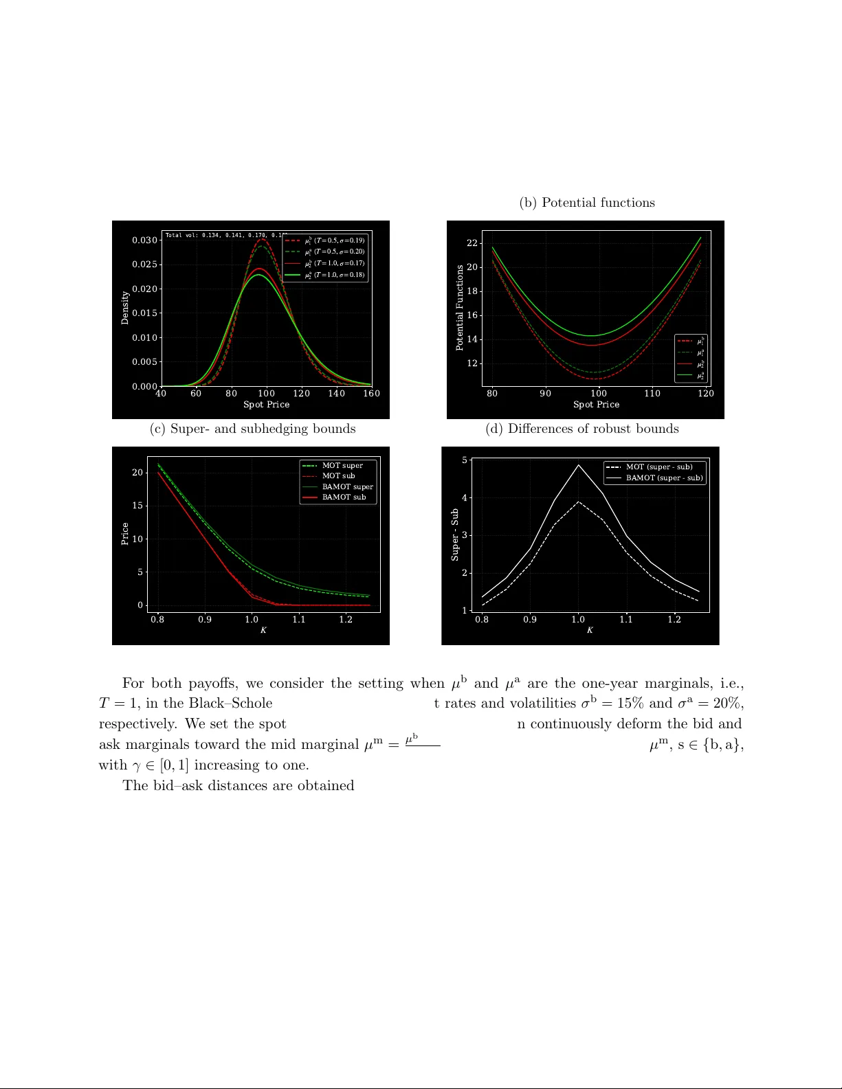
Bid–Ask Martingale Optimal T ransp ort Bry an Liang ∗ Marcel Nutz † Sh unan Sheng ‡ V alen tin Tissot-Daguette § Marc h 27, 2026 Abstract Martingale Optimal T ransp ort (MOT) pro vides a framew ork for robust pricing and hedging of illiquid deriv ativ es. Classical MOT enforces exact calibration of mo del marginals to the mid-prices of v anilla options. Motiv ated by the industry practice of ﬁtting bid and ask marginals to v anilla prices, we introduce a relaxation of MOT in which mo del-implied volatilities are only required to lie within observed bid–ask spreads; equiv alen tly , mo del marginals lie b et w een the bid and ask marginals in con v ex order. The resulting Bid–Ask MOT (BAMOT) yields realistic price b ounds for illiquid deriv ativ es and, via strong duality , can b e interpreted as the sup erhedging price when short and long p ositions in v anilla options are priced at the bid and ask, resp ectiv ely . W e further establish conv ergence of BAMOT to classical MOT as bid–ask spreads v anish, and quan tify the conv ergence rate using a nov el distance in trinsically linked to bid–ask spreads. Finally , we supp ort our ﬁndings with several synthetic and real-data examples. Keyw ords Martingale Optimal T ransp ort, Financial Deriv atives, Robust Hedging, Bid–Ask F riction AMS 2020 Sub ject Classiﬁcation 91G20, 62P05, 60G42 JEL Classiﬁcation G11, G13, D52 Ac kno wledgmen ts W e w ould lik e to thank Bruno Dupire, Martin F orde, Sergey Nadto chiy , W alter Sc hacherma yer, Mete Soner, and Josef T eichmann for helpful discussions on this topic. Sh unan Sheng is supp orted by a Blo om berg Quantitativ e Finance Ph.D. F ellowship. 1 In tro duction Martingale Optimal T ransp ort (MOT) [ 3 , 6 , 7 , 19 , 22 ] oﬀers a p ow erful framework to price and hedge illiquid deriv atives. Consider a claim H con tingen t on the evolution of a liquidly traded asset ( X t ) 0 ≤ t ≤ T up to some ﬁxed maturity T > 0. Supp ose also that the static hedging instrumen ts consist of all T -v anilla options (i.e., all put and call options with maturity T and an y strike K ≥ 0), in addition to dynamic trading in ( X t ) 0 ≤ t ≤ T . Absent market frictions, one classically extracts a ∗ Quan titative Researc h, Oﬃce of the CTO, Bloomberg. Email: bliang17@blo om berg.net. † Colum bia Universit y , Departments of Statistics and Mathematics. Research supp orted by NSF Grants DMS- 2106056, DMS-2407074. Email: mnutz@colum bia.edu. ‡ Colum bia Univ ersity , Department of Statistics. Email: ss6574@columbia.edu. Researc h initiated during an in ternship at Blo om berg. § Quan titative Researc h, Oﬃce of the CTO, Bloomberg. Email: vtissotdague@blo om berg.net 1 unique risk-neutral distribution µ consisten t with the Black–Sc holes implied volatilit y (IV) skew σ ( K, T ). Indeed, assuming zero carry , we hav e by [11] that µ (d K ) d K = ∂ 2 K c ( K, T ) , c ( K, T ) := c BS ( K, T , σ ( K, T )) , (1) where c BS ( K, T , σ ) is the price of the ( K, T ) call option in the Black–Sc holes mo del with volatilit y σ . MOT then considers the set of all arbitrage-free mo dels (martingale measures) for ( X t ) 0 ≤ t ≤ T suc h that the marginal law µ Q T of X T under Q coincides with µ , leading to the primal (or measure) problem sup Q ∈Q ( µ ) E Q [ H ] , Q ( µ ) =  Q | martingale measure, µ Q T = µ  . (2) A similar logic applies when the static hedging instruments are a v ailable at multiple maturities T 1 , . . . , T N , leading to marginal constraints µ Q T i = µ i for i = 1 , . . . , N . T o wit, MOT requires admissible mo dels to exactly match the market’s implied volatilit y (IV) skews, thus imp osing hard constrain ts on the marginal distributions. The dual of MOT, discussed in more detail b elow, is a semi-static sup erhedging problem, whic h assumes that v anilla options can b e b ought and sold at the prices implied by those IV skews, with no bid–ask friction. 1.1 Bid–Ask F riction The present work develops an extension of MOT that accoun ts for the presence of bid–ask spreads for v anilla prices in real markets. Indeed, in practice, v anilla options are often represented in terms of bid and ask IV skews σ b ( K, T ) ≤ σ a ( K, T ). Then a martingale measure Q is consistent with the options mark et if and only if the implied v olatilities σ Q ( K, T ) that it generates (see Fig. 1) satisfy σ b ( K, T ) ≤ σ Q ( K, T ) ≤ σ a ( K, T ) , K ≥ 0 . (3) Of course, order b ooks only con tain quotes for ﬁnitely many strikes at any giv en moment. Data v endors provide bid/ask IV skews by in terp olating/extrapolating the a v ailable quotes. As detailed in Section 2.1, a common approac h for this task is to ﬁt bid and ask mar ginal distributions µ b , µ a within a parametric family to the a v ailable quotes. This motiv ates the primal formulation of our problem, which replaces the single (mid-price) marginal µ of the MOT problem (2) b y a set of p ossible marginals determined via µ b and µ a as follo ws. 1.2 Primal F orm ulation T o b e consis ten t with the bid and ask IVs, the p ossible marginals µ Q T = La w Q ( X T ) for the asset price X T m ust satisfy certain conv ex order constraints. Indeed, (3) implies E µ b [( X − K ) + ] = c BS ( K, T , σ b ( K, T )) ≤ c BS ( K, T , σ Q ( K, T )) = E µ Q T [( X − K ) + ] for all K ≥ 0 since c BS ( K, T , σ ) is nondecreasing in σ . This means that µ b and µ Q T are in c onvex or der, denoted µ b ⪯ c µ Q T , by the prop erty of conv ex order recalled in (7) b elo w. Similarly , µ Q T ⪯ c µ a . This leads us to form ulate the following extension of the MOT problem (2) , whic h w e call the Bid–Ask Martingale Optimal T r ansp ort (BAMOT) problem: sup Q ∈Q ( µ b ,µ a ) E Q [ H ] , Q ( µ b , µ a ) =  Q | martingale measure, µ b ⪯ c µ Q T ⪯ c µ a  . (4) 2 Figure 1: Bid, mo del, and ask implied volatilit y skews for S&P 500 Index (SPX) options expiring on 03-21-2025, as of 02-27-2025. More generally , we will consider a version of this problem with multiple maturities T 1 , . . . , T N . In con trast to its classical counterpart, BAMOT captures mo del uncertaint y ab out the underlying asset ( X t ) 0 ≤ t ≤ T arising not only from its price dynamics, but also from its marginal distributions: while MOT prescrib es the marginal µ exactly , the bid and ask marginals merely imply inequality constrain ts for the marginal distribution of the asset. In particular, BAMOT is nontrivial ev en for claims that dep end only on X T , suc h as a digital option, whereas MOT simply prices them by taking exp ectation under µ . In general, the v alue of (4) is no less than the v alue of (2) (for any µ b ⪯ c µ ⪯ c µ a ), reﬂecting that the seller of the claim faces additional mo del uncertaint y . 1.3 Dual F orm ulation Next, we consider the eﬀect of bid–ask spreads from the hedging p ersp ectiv e. In the classical MOT setting with a single marginal µ , the dual (or p ortfolio) problem aims at minimizing the sup erhedging cost of the claim H , given by inf { µ ( ψ ) | ψ ∈ Ψ( H ) } , Ψ( H ) = n ψ ∈ L 1 ( µ ) | ∃ ∆ such that P&L H ψ , ∆ ≥ 0 o . Here ∆ is a dynamic hedging strategy trading in the asset ( X t ) 0 ≤ t ≤ T and P&L H ψ , ∆ ( X ) = ψ ( X T ) + (∆ • X ) T − H is the proﬁt and loss resulting from three terms: the static hedge ψ , whic h is constructed from v anilla options at cost µ ( ψ ) := R ψ d µ , dynamic (self-ﬁnancing) trading according to ∆ leading to the sto c hastic integral (∆ • X ) T , and selling the claim H . F or the static hedge ψ , it is suﬃcient (cf. [22]) to lo ok for proﬁles of the form ψ ( x ) = γ $ + Z R + ( x − K ) + λ (d K ) (5) where γ $ is a cash amoun t and λ is a signed measure describing the weigh ts of a call options p ortfolio (as even tual p ositions in the forward contract can b e absorb ed b y the delta hedge). 3 Gran ted that F ubini’s theorem applies, the cost of ψ reads µ ( ψ ) = γ $ + R R + c ( K, T ) λ (d K ), where c ( K, T ) = E µ [( X − K ) + ]. In our problem formulation, w e keep the assumption that trading in ( X t ) 0 ≤ t ≤ T is frictionless but highligh t the static proﬁle ψ , whic h is now exp osed to the bid–ask frictions in the options market. W e naturally assume that static hedging is limited to put and call options (and the forw ard). In fact, puts would b e redundan t given calls and the forw ard, hence we may supp ose again that ψ consists of a cash amount and a p ortfolio of call options as in (5) . In the presence of bid–ask spreads, we need to separate the con tracts that w ere b ough t from those that were sold. T o this end, consider the Jordan decomp osition λ = λ + − λ − of the p ortfolio weigh ts in to nonnegative measures λ ± . W e can then decomp ose the static proﬁle as ψ = ψ a − ψ b , ψ a ( x ) = γ $ + Z R + ( x − K ) + λ + (d K ) , ψ b ( x ) = Z R + ( x − K ) + λ − (d K ) . Since λ ± are nonnegativ e, b oth ψ a , ψ b are c onvex proﬁles, the ﬁrst b eing b ough t at the ask and the second sold at the bid. W riting c b ( K, T ) and c a ( K, T ) for the bid and ask call option prices, the cost of ψ b ecomes γ $ + Z R + c a ( K, T ) λ + (d K ) − Z R + c b ( K, T ) λ − (d K ) . Figure 2 displa ys the bid–ask spread for put and call options on the S&P 500 Index (SPX) across strik es and maturities as of the close of 02-07-2025. As can b e seen, the spreads are non-negligible, ev en for liquid underlyings suc h as SPX. With bid and ask marginals µ b ⪯ c µ a as in Section 1.2, we can write the cost of the static proﬁle succinctly as µ a ( ψ a ) − µ b ( ψ b ). Figure 2: Bid–ask spread ($) of S&P 500 Index (SPX) options as of 02-07-2025. More generally , we formulate our dual problem ov er p airs ψ b , a = ( ψ a , ψ b ) of con vex functions, with ψ a corresp onding to call options b ough t (plus a cash p osition) and ψ b corresp onding to call options sold. 1 W riting cost( ψ b , a ) = µ a ( ψ a ) − µ b ( ψ b ) for ψ b , a = ( ψ a , ψ b ) , 1 W e do not insist that ψ a − ψ b b e a Jordan decomp osition. How ev er, a Jordan decomposition has the minimal cost µ a ( ψ a ) − µ b ( ψ b ) among all decomp ositions in to con v ex functions. 4 w e arrive at the dual formulation inf ψ b , a ∈ Ψ b , a ( H ) cost( ψ b , a ) , (6) where Ψ b , a ( H ) =  ψ b , a = ( ψ a , ψ b ) con vex | ∃ ∆ suc h that P&L H ψ a − ψ b , ∆ ≥ 0  . Our strong duality result (Theorem 3.4) will prov e that the optimal sup erhedging cost (6) coincides with the v alue of the primal problem (4) . The presence of bid–ask spreads increases the v alue of the dual problem as cost ( ψ b , a ) ≥ µ ( ψ a − ψ b ) for any µ b ⪯ c µ ⪯ c µ a . W e will see in Section 5 that the v alue may diﬀer substan tially from the price under the mid-marginal µ = ( µ a + µ b ) / 2 given real mark et data. In con trast to the dual in classical MOT, (6) is non trivial ev en for v anilla claims H = h ( X T ). Ev en if h = ψ 0 − ψ 1 is itself a diﬀerence of con v ex functions, e.g., via Jordan decomp osition, there ma y b e conv ex pairs ( ψ a , ψ b ) =: ψ b , a suc h that ψ a − ψ b ≥ h and cost ( ψ b , a ) < µ a ( ψ 0 ) − µ b ( ψ 1 ). That is, the Jor dan de c omp osition c an b e sub optimal for the dual problem. A concrete example is shown in Fig. 8, where the risk-rev ersal strategy h ( x ) = ( x − 1 . 05) + − (0 . 95 − x ) + is optimally sup erhedged by a linear combination of thr e e call options. 1.4 Con tributions On the conceptual side, we introduce a no vel generalization of martingale optimal transp ort that is consisten t with bid–ask spreads for v anilla options. While directly using order b o ok data of bid and ask quotes would lead to a general linear programming problem, a k ey observ ation is that the existing market practice of ﬁtting bid and ask marginal distributions op ens the do or to a tractable form ulation in the realm of optimal transp ort. On the theoretical side, in Section 2, we ﬁrst formalize the corresp onding primal (transp ort) problem and the dual (sup erhedging) problem. W e also describ e more precisely the relation b et w een discrete bid and ask quotes in order b o oks and the corresp onding idealized marginal distributions. In Sec tion 3, we then establish strong duality: the BAMOT primal v alue (4) coincides with the dual sup erhedging cost (6) for any upp er semicontin uous pay oﬀ h ( X T 1 , . . . , X T N ) with, at most, linear growth. Metho dologically , w e ﬁrst show strong duality for the single-maturity case by a Hahn–Banac h argument (Theorem 3.2). This case corresp onds to sup erhedging a pa y oﬀ h ( X T ) b y a diﬀerence ψ a − ψ b of conv ex functions of X T and is genuinely nov el compared to MOT. W e then show strong duality for the general, m ulti-maturit y case (Theorem 3.4) by combining the single-p eriod result with MOT dualit y via a minimax argument. Section 4 contin ues the theoretical analysis by studying the relationship b et w een BAMOT and the classical MOT problem without bid–ask spreads. Prop osition 4.1 establishes consistency , in the sense that the BAMOT v alue conv erges to the MOT limit as the bid–ask spread v anishes. By dualit y , the optimal sup erhedging costs then also conv erge. In the imp ortan t sp ecial case of a single maturit y , we further pro vide a quantitativ e analysis. T o that end, we in tro duce a no v el metric, the bid–ask distanc e , which aligns with the spreads of quoted v anilla options and captures the conv ex ordering b etw een marginals. W e then sho w a linear rate of conv ergence of the BAMOT price for pa y oﬀs, which are diﬀerences of conv ex functions (Prop osition 4.5), and a square-ro ot rate for upp er semicon tin uous pa yoﬀs (Prop osition 4.6). Both rates are shown to b e numerically sharp in examples, namely , for a risk-reversal strategy and an at-the-money digital option (Section 5.3). 5 On the practical side, we provide analytical and computational examples illustrating the form ulation and its implications. In Section 5.1, we derive a closed-form solution for digital call options in a one-sided market and v alidate the impact of bid–ask frictions using real mark et data on the S&P 500 Index (SPX). Our ﬁndings rev eal that the common practice of pricing digital options using the mid-price marginal can substan tially underestimate (sup erhedging) prices relative to BAMOT in the presence of bid–ask frictions. In Section 5.2, w e compare BAMOT sup er- and subhedging b ounds for a forw ard-start pay oﬀ with those obtained under classical MOT. Finally , in Section 5.3, w e do cument the con vergence b eha vior as bid–ask spreads shrink for a risk-reversal strategy and an at-the-money digital call option. 1.5 Related Literature Addressing mark et friction arising from bid–ask spreads has a long history in robust ﬁnance (see, e.g., [ 2 , 10 , 13 , 17 , 26 ] and the references therein). T ransaction cost analysis w as pioneered by [ 26 ], whic h introduced a sublinear pricing op erator to capture the bid–ask spread of trading a contingen t claim. It is shown that the sup erhedging cost of the claim agrees with the maxim um contract v alue among all martingale measures consisten t with the bid and ask prices of the hedging instruments. Closer to our robust ﬁnance framework, [ 15 ] utilized sublinear op erators to describ e the cost of static hedging and established general duality results that also include prop ortional transaction costs for dynamic hedging. In the present work, we assume that costs for trading in the underlying are negligible relative to the bid–ask spreads of the v anilla options, as is typically satisﬁed in practice for mo derate trading frequency . Moreov er, w e fo cus on a particular mo del close to industry practices, rather than aiming for general results. A related duality was recently established by [ 17 ] in the con text of generalized Limit Order Bo oks (LOB) inv olving bundles of sec urities. Ov er the past several y ears, researc hers ha v e increasingly leveraged MOT to address market frictions. Ho w ever, many works fo cus on capturing bid–ask spreads in less liquid exotic options [ 18 , 21 ]. In particular, these studies assume that v anilla options can still b e b ought and sold at a unique price, leading to exact calibration of the marginal distributions. Other approaches within the MOT framework sp eciﬁcally accommo date the uncertaint y in inferring marginal distributions from mark et spreads. F or instance, [ 24 ] in tro duced η -market mo dels , which utilize a uniform tolerance parameter η for all v anilla options, eﬀectively resulting in a constant bid–ask spread across all strik es. Alternatively , [ 40 ] directly optimized ov er a set of martingale measures whose marginals reside within a pre-deﬁned ε -tolerance set. Nonetheless, selecting appropriate hyperparameters for η and ε is often c hallenging in practice. By con trast, the bid and ask marginals imp osed in the presen t w ork are motiv ated by industry practice and can b e directly calibrated to the bid and ask prices observ ed in market data. W e mention that [ 32 ] to ok steps tow ard addressing these concerns, alb eit from a more empirical p erspective: the authors prop osed a neural net w ork-based approach to solve the dual problem, incorp orating an ob jective function that explicitly accounts for the discrepancy b et w een bid and ask prices. In a diﬀerent direction, not directly related to optimal transp ort, the mo deling of bid–ask spreads using separate marginals has b een explored through “low er” and “upp er” measures by [ 28 , 29 ]. In these studies, p ositions are group ed b y directional sentimen t: bullish views (long calls, short puts) are v alued under the upp er measure, while b earish views (long puts, short calls) utilize the lo w er measure. Consequently , the ask prices for calls and puts originate from diﬀeren t distributions. 6 While empirically robust, this framew ork do es not provide the uniﬁed marginal constraints required for MOT, where bid and ask prices are reco v ered from a single consistent pair of distributions. Finally , our results in Section 4 ab out conv ergence of BAMOT for shrinking bid–ask spreads are related to the literature on the stability of MOT, that is, its b eha vior as a function of the giv en marginals. Here [ 27 ] derived the stability of the left-curtain coupling, thereby establishing stability results for MOT. Indep endently , [ 5 , 38 ] obtained contin uit y of the v alue functions and optimal couplings b y exploiting the adapted W asserstein top ology . Subsequen t w orks [ 4 , 31 ] further conﬁrmed this top ology as the natural framew ork for studying stability in MOT. On the computational side, [ 20 ] inv estigated stabilit y in order to provide guaran tees for n umerical metho ds when the marginals are appro ximated discretely . 1.6 Notation Let C L ( R N + ) b e the Banach space of con tin uous functions f : R N + → R with linear growth, endow ed with the norm ∥ f ∥ L := sup x ∈ R N + | f ( x ) | 1 + ∥ x ∥ . In tro duce also the larger set USC L ( R N + ) of upper semicon tinuous (u.s.c.) functions with linear gro wth, and the smaller set CVX L ( R N + ) of con v ex functions with linear growth. When N = 1, we drop the dep endence on the am bien t space and simply write C L , CVX L , USC L . Let P 1 ( R N + ) b e the set of probability measures on R N + with ﬁnite ﬁrst moment, and abbreviate again P 1 = P 1 ( R + ). The 1-W asserstein distance W 1 ( µ, ν ) is deﬁned via W 1 ( µ, ν ) = inf R ∥ x − y ∥ P (d x, d y ) , where the inﬁmum is taken ov er all couplings P of ( µ, ν ), i.e., all P ∈ P ( R N + × R N + ) with marginals ( µ, ν ). Integrals are denoted, interc hangeably , b y µ ( f ) = E µ [ f ] = Z f d µ. W e say that µ, ν ∈ P 1 are in c onvex or der ( µ ⪯ c ν ) if µ ( ψ ) ≤ ν ( ψ ) for all ψ ∈ CVX L . In fact, it is suﬃcien t to v erify the latter inequalit y for call pay oﬀs, provided that the measures hav e identical barycen ters µ ⪯ c ν ⇐ ⇒ E µ [ X ] = E ν [ X ] and E µ [( X − K ) + ] ≤ E ν [( X − K ) + ] ∀ K ≥ 0 . (7) See, e.g., [ 34 ] for further bac kground on con v ex order, and in particular [ 34 , Theorem 3.A.1] for the ab o v e equiv alence. Organization The remainder of the pap er is organized as follo ws. Section 2 presents a practitioners’ construction of bid–ask marginals and formulates the primal and dual BAMOT problems. Section 3 establishes strong duality . Section 4 prov es consistency and derives the conv ergence rate in the single-maturit y case N = 1. Section 5 presen ts illustrative examples and numerical results. W e conclude by discussing p ossible directions for future w ork in Section 6. Section A discusses the existence of bid and ask measures. T ec hnical pro ofs and other complemen tary materials are presen ted in Sections B and C. 7 2 Bid–Ask MOT This section introduces the primal (measure) problem and the dual (p ortfolio) problem of BAMOT in detail. Both problems dep end crucially on the assumption of bid and ask marginals that induce the prices of liquidly traded call and put options. W orking with such marginals is mark et practice, oﬀering a ﬂexible metho d to calibrate bid–ask implied v olatilit y sk ews, while ruling out static arbitrage. Fig. 1 replicates a typical market interface for implied volatilit y skews, suc h as the OVD V function on the Blo omberg T erminal. On the other hand, a snapshot of real-world order b ook data ma y contain quotes that cannot b e exactly repro duced by tw o distributions. The next subsections explain how practitioners typically calibrate bid and ask marginals to quotes; see [ 12 ] and the OVD V do cumen tation av ailable on the Blo om berg T erminal. 2.1 Bid and Ask Marginals Next, we describ e a common pro cedure used by practitioners to construct bid and ask marginals b y calibrating to bid and ask quotes of out-of-the-money (OTM) put and call options. 2 Fix a maturity T , let F T , x 0 denote, resp ectiv ely , the forw ard and spot price of the underlying, let { K m } m ∈ [ M ] b e the set of av ailable strikes, and let { OTM a ( K m , T ) } m ∈ [ M ] and { ϑ a ( K m , T ) } m ∈ [ M ] denote, resp ectiv ely , the ask prices and V egas of the corresp onding OTM options (put if x 0 < K m and call otherwise). Practitioners then select a parametric family of densities { ϕ θ | θ ∈ Θ } , where Θ is chosen so that the forward price is matched (i.e., R xϕ θ ( x ) d x = F T for all θ ∈ Θ), and solve the optimization θ a ∈ arg min θ ∈ Θ X m ∈ [ M ]     OTM a ( K m , T ) − OTM θ ( K m , T ) ϑ a ( K m , T )     2 , where OTM θ ( K, T ) denotes the OTM option price under ϕ θ . Here pricing errors are weigh ted by V egas to appro ximately con v ert price discrepancies into errors in implied v olatilities (IVs). The resulting distribution µ a (d x ) = ϕ θ a ( x ) d x is referred to as the calibrated ask mar ginal . One then p erturbs the ﬁtted parameters θ a to obtain bid parameters θ b that matc h bid quotes, and sets µ b (d x ) = ϕ θ b ( x ) d x as the corresp onding bid mar ginal . In particular, one uses a p erturbation such that µ b ⪯ c µ a to rule out static arbitr age . A common choice of parametric family is mixtures of log-normal densities [ 12 ]. Supp ose the ask marginal is calibrated as a log-normal mixture with J comp onen ts, i.e., ϕ a ( x ) = J X j =1 w j ϕ BS ( x ; z j , σ a j ) , J X j =1 w j = 1 , where ϕ BS ( · ; z , σ ) denotes the densit y of a log-normal distribution with mean and v olatilit y parameters ( z , σ ) ∈ R 2 + . The bid marginal is then constructed b y scaling down the volatilit y parameters, while k eeping the remaining parameters unchanged: ϕ b ( x ) = J X j =1 w j ϕ BS ( x ; z j , σ b j ) , 2 OTM options are chosen as they are usually more liquid and therefore lead to more reliable and consisten t quotes. 8 for some calibrated σ b j ≤ σ a j , j ∈ [ J ]. Giv en multiple maturities T 1 ≤ T 2 ≤ · · · ≤ T N , we apply the ab o v e pro cedure at each maturity and obtain bid and ask marginals µ b i , µ a i suc h that µ b i ⪯ c µ a i for eac h i ∈ [ N ] := { 1 , . . . , N } . F or simplicity , assume zero interest rate and no carry cost. 3 In this case, F T i = x 0 for all i ∈ [ N ]. The absence of c alendar arbitr age across maturities suggests the cross-maturit y condition µ b i ⪯ c µ a j for an y 1 ≤ i ≤ j ≤ N . Indeed, if there exists K ≥ 0 suc h that E µ b i [( X − K ) + ] > E µ a j [( X − K ) + ], then one could sell the ( K, T i ) call at a price at least E µ b i [( X − K ) + ] and buy the ( K, T j ) call at a price at most E µ a j [( X − K ) + ]; together with dynamic trading in the underlying, this yields an arbitrage. The ab ov e discussion motiv ates the following assumption, which we adopt throughout the pap er. Assumption 2.1. There exist bid and ask marginals µ b = ( µ b 1 , . . . , µ b N ) and µ a = ( µ a 1 , . . . , µ a N ) with ﬁnite ﬁrst momen t, which determine the bid and ask prices of all call and put options with the resp ectiv e maturities and satisfy µ b i ⪯ c µ a j , ∀ 1 ≤ i ≤ j ≤ N . (8) Remark 2.2. (a) Condition (8) rules out butterﬂy arbitrage; for an y i ∈ [ N ], K ∈ R + , E µ a i [( X − K − ) + ] − 2 E µ b i [( X − K ) + ] + E µ a i [( X − K + ) + ] ≥ 0 , K ± = K ± δ , δ > 0 . (9) Indeed, E µ b i [( X − K ) + ] ≤ E µ a i [( X − K ) + ] by (8) , so the left-hand side of (9) is b ounded from b elo w b y E µ a i [ B ( X , K )], with the butterﬂy spread B ( x, K ) = ( x − K − ) + − 2( x − K ) + +( x − K + ) + . Since B ( · , K ) ≥ 0, its price under µ a i (and hence under an y admissible bid–ask calibration) m ust b e nonnegative. (b) By a suitable choice of the bid and ask marginals, our framework co v ers situations in which the pa y oﬀ dep ends on maturities for which v anilla options are not liquidly traded. F or example, if N = 2 and the pay oﬀ is H = h ( X T 1 , X T 2 ), while v anillas are av ailable at T 2 but not at T 1 , one ma y tak e µ b 1 := δ x 0 and µ a 1 := µ a 2 , thereb y lea ving the T 1 -marginal eﬀectiv ely unconstrained, while still enforcing the cross-maturity condition (8) . Such a situation naturally arises when the pro duct references an intermediate ﬁxing date, e.g., forw ard-start, whereas market quotes are only liquid at coarser maturities. 2.2 Primal (Measure) Problem Fix maturities T 1 ≤ T 2 ≤ · · · ≤ T N with corresp onding bid marginals µ b = ( µ b 1 , . . . , µ b N ) and ask marginals µ a = ( µ a 1 , . . . , µ a N ). W e write X 1 , . . . , X N for the canonical pro cess represen ting the sp ot price, where we identify X i = X T i for notational simplicity . By con v en tion, the initial price X 0 := x 0 ∈ R + is deterministic. Th us, a martingale me asur e is a probability measure Q on R N + suc h that ( X i ) 0 ≤ i ≤ N is a Q -martingale. The set of c alibr ate d martingale measures is Q ( µ b , µ a ) := n Q | martingale measure , µ b i ⪯ c µ Q i ⪯ c µ a i , i ∈ [ N ] o , (10) 3 With positive interest rates and/or dividends, the marginals µ b i , µ a i should be calibrated from disc ounte d, dividend- adjuste d quotes . 9 where µ Q i denotes the i -th marginal distribution of Q . Fix a contingen t claim H = h ( X 1 , . . . , X N ) for some pay oﬀ function h ∈ USC L ( R N + ). Then the primal (or me asur e ) problem is deﬁned as P ( h ) := sup Q ∈Q ( µ b ,µ a ) E Q [ h ( X 1 , . . . , X N )] . (11) W e observe that Assumption (8) ⇐ ⇒ Q ( µ b , µ a )  = ∅ . Indeed, deﬁne µ i = min j ≥ i µ a j , where the inﬁmum is with resp ect to the con v ex order. Then µ i ⪯ c µ j for all i ≤ j and µ b i ⪯ c µ i ⪯ c µ a i for all i . By Strassen’s theorem, the former implies the existence of a martingale measure Q with marginals µ = ( µ 1 , . . . , µ N ), and Q ∈ Q ( µ b , µ a ) b y the latter. Con v ersely , if Q ∈ Q ( µ b , µ a ), let ( µ 1 , . . . , µ N ) b e its vector of marginals. The martingale prop ert y implies µ i ⪯ c µ j for all i ≤ j and then Q ∈ Q ( µ b , µ a ) implies (8). Remark 2.3. Consider again the low er en v elop e µ a i := min j ≥ i µ a j used in the ab ov e argumen t, and similarly the upp er env elop e µ b i := max j ≤ i µ b j . W e see that (8) , and in turn Q ( µ b , µ a )  = ∅ , are equiv alent to µ b i ⪯ c µ a i for all i . That is, the prices of conv ex pay oﬀs with resp ect to the low er and upp er env elop es do not cross, as illustrated in Fig. 3 for an illiquid, in-the-money call on the S&P 500 Index (SPX). Figure 3: T erm structure of S&P 500 Index (SPX) call options struc k at K = 5550 as of 2025-02-27, and corresp onding price env elop es. 2.3 Dual (P ortfolio) Problem Consider a pay oﬀ function h ∈ USC L ( R N + ), meaning that the claim is h ( X 1 , . . . , X N ), and static hedging instrumen ts ψ = ( ψ 1 , . . . , ψ N ) with pa yoﬀs ψ i ( X i ). Moreov er, let ∆ = (∆ 1 , . . . , ∆ N − 1 ) b e a progressiv ely measurable trading strategy (delta hedge), that is, ∆ i is a measurable function of X 1 , . . . , X i . The proﬁt and loss asso ciated with ψ , ∆ , h is deﬁned as P&L h ψ , ∆ ( x 1 , . . . , x N ) = N X i =1 ψ i ( x i ) + N − 1 X i =1 ∆ i ( x 1 , . . . , x i )( x i +1 − x i ) − h ( x 1 , . . . , x N ) . 10 As customary in MOT [3, 22], it is suﬃcien t to lo ok for static proﬁles of the form ψ i ( x ) = γ $ i + Z R + ( x − K ) + λ i (d K ) , noting that even tual positions in the forw ard con tract can b e absorb ed by the delta hedge. In our dual problem, the delta hedges are arbitrary , whereas the static p ositions are expressed as the diﬀerence ψ i = ψ a i − ψ b i of con vex functions. Here ψ a i corresp onds to a combination of call options with maturity T i that are b ought, while ψ b i corresp onds to call options which are sold. (Put options are redundant given calls and the forw ard contract, hence can b e ignored.) F or brevity , w e combine these functions into a vector ψ b , a = ( ψ a , ψ b ) = ( ψ a 1 , . . . , ψ a N , ψ b 1 , . . . , ψ b N ) ∈ CVX 2 N L whose total cost is cost( ψ b , a ) = N X i =1 µ a i ( ψ a i ) − µ b i ( ψ b i ) . W e denote the set of all admissible sup erhedging strategies by Ψ b , a ( h ) = n ( ψ a , ψ b ) ∈ CVX 2 N L | ∃ ∆ s.t. P&L h ψ a − ψ b , ∆ ≥ 0 o ; (12) here and b elo w, it is tacitly understo od that ∆ is progressively measurable. The dual (or p ortfolio ) problem is then deﬁned as D ( h ) := inf ψ b , a ∈ Ψ b , a ( h ) cost( ψ b , a ) , (13) The in terpretation is straightforw ard: sell one unit of h ; at each maturity T i , buy a conv ex proﬁle ψ a i priced at the ask, sell another proﬁle ψ b i at the bid, and hold ∆ i shares of the underlying asset to hedge against p oten tial losses and minimize cost. 3 Dualit y The goal of this section is to show the strong duality P ( h ) = D ( h ), where P ( h ) and D ( h ) denote the v alues of the primal (11) and dual (13) problems, resp ectiv ely . W e ﬁrst state the weak dualit y P ( h ) ≤ D ( h ), which is straightforw ard. Lemma 3.1 (W eak Duality) . We have P ( h ) ≤ D ( h ) for al l h ∈ USC L ( R N + ) . Pr o of. Let Q ∈ Q ( µ b , µ a ) and ψ b , a = ( ψ a , ψ b ) ∈ Ψ b , a ( h ), and let ∆ b e a corresp onding dynamic strategy such that P&L h ψ a − ψ b , ∆ ≥ 0. Since Q is a martingale measure with µ b i ⪯ c µ Q i ⪯ c µ a i , and ψ a i , ψ b i are con vex with linear growth, we deduce E Q [ h ( X 1 , . . . , X N )] ≤ E Q  N X i =1 ψ a i ( X i ) − ψ b i ( X i )  + E Q  N − 1 X i =1 ∆ i ( X 1 , . . . , X i )( X i +1 − X i )  = N X i =1 µ Q i ( ψ a i ) − µ Q i ( ψ b i ) ≤ N X i =1 µ a i ( ψ a i ) − µ b i ( ψ b i ) = cost( ψ b , a ) . 11 Here we hav e used that the discrete sto c hastic integral has v anishing exp ectation. Indeed, the negativ e part of the terminal v alue of this lo cal martingale is Q -in tegrable due to the sup erhedging prop ert y and the linear gro wth of h , and that implies that it is a true martingale [ 25 , Theorem 2]. The result follows by taking supremum ov er Q and inﬁm um ov er ψ b , a ∈ Ψ b , a ( h ). The nontrivial direction of the strong duality will b e established in tw o steps. W e ﬁrst fo cus on the single-maturity case N = 1, where w e pro v e strong duality from ﬁrst principles via a Hahn–Banac h argumen t. W e then sho w the result for the general case b y combining the strong dualit y of classical MOT with the single-maturit y case. 3.1 Single Maturit y Let N = 1 and consider the single maturity T 1 > 0 as well as corresp onding bid and ask marginals µ b , µ a ∈ P 1 satisfying µ b ⪯ c µ a . W e sligh tly abuse notation b y writing µ s for µ s 1 , etc., and iden tifying martingale measures with their marginal µ at T 1 (rather than using the full martingale measure δ x 0 ⊗ µ ). Then the primal problem (11) b oils down to P ( h ) = sup µ ∈Q ( µ b ,µ a ) µ ( h ) , Q ( µ b , µ a ) = { µ ∈ P 1 | µ b ⪯ c µ ⪯ c µ a } , (14) where h ∈ USC L is the pa y oﬀ function of a T 1 -claim h ( X 1 ). On the other hand, the dual problem (13) b ecomes D ( h ) = inf ψ b , a ∈ Ψ b , a ( h ) cost( ψ b , a ) , cost( ψ b , a ) = µ a ( ψ a ) − µ b ( ψ b ) , Ψ b , a ( h ) = { ψ b , a = ( ψ a , ψ b ) ∈ CVX 2 L | ψ a − ψ b ≥ h } . That is, D ( h ) is the cost of the cheapest static sup erhedging p ortfolio of h , given by the diﬀerence of con v ex functions. Observe that P ( h ) = µ a ( h ) = D ( h ) if h is con v ex, and P ( h ) = µ b ( h ) = D ( h ) when h is concav e. The next result extends strong duality to general pay oﬀs. Theorem 3.2 (Strong Duality , N = 1) . F or al l h ∈ USC L , we have P ( h ) = sup µ ∈Q ( µ b ,µ a ) µ ( h ) = inf ψ ∈ Ψ b , a ( h ) cost( ψ ) = D ( h ) . Mor e over, ther e exists a primal optimizer µ ⋆ ∈ Q ( µ b , µ a ) . Pr o of. The w eak duality P ( h ) ≤ D ( h ) w as shown in Lemma 3.1. T o show the reverse inequality , w e ﬁrst assume that h ∈ C L ( R + ). Our aim is to construct a measure µ ⋆ ∈ Q ( µ b , µ a ) suc h that µ ⋆ ( h ) = D ( h ). Since we already kno w that µ ⋆ ( h ) ≤ P ( h ) ≤ D ( h ), this will imply that P ( h ) = D ( h ) and µ ⋆ is a maximizer. Step 1. W e sho w that D : C L ( R + ) → R is a sublinear functional. Clearly D ( λf ) = λD ( f ) for all λ > 0 and f ∈ C L ( R + ). Note also that D ( λ ) = λ for all λ ∈ R , using, e.g., ψ ≡ ( λ, 0) ∈ Ψ b , a ( λ ). Moreo v er, D is subadditive, D ( f + f ′ ) ≤ D ( f ) + D ( f ′ ) ∀ f , f ′ ∈ C L ( R + ) . 12 Indeed, Ψ b , a ( f ) + Ψ b , a ( f ′ ) ⊆ Ψ b , a ( f + f ′ ), whic h gives D ( f + f ′ ) = inf ψ ∈ Ψ b , a ( f + f ′ ) cost( ψ ) ≤ inf ψ ∈ Ψ b , a ( f ) , ψ ′ ∈ Ψ b , a ( f ′ ) cost( ψ + ψ ′ ) = D ( f ) + D ( f ′ ) since cost( · ) is linear. This completes the pro of that D is sublinear. Step 2. Consider the one-dimensional linear subspace M := { λh : λ ∈ R } ⊆ C L ( R + ) and in tro duce the linear functional ℓ ( λh ) := λD ( h ) on M . Then ℓ ( λh ) = D ( λh ) ∀ λ > 0 due to the p ositiv e homogeneity of D . Moreo v er, ℓ ( − λh ) ≤ D ( − λh ) for all λ ≥ 0, as follo ws from ℓ ( λh ) + ℓ ( − λh ) = ℓ (0) = 0 = D (0) = D ( λh − λh ) ≤ D ( λh ) + D ( − λh ) . Hence ℓ ( f ) ≤ D ( f ) for all f ∈ M , that is, ℓ is dominated b y D on M . By the Hahn–Banac h Dominated Extension Theorem, ℓ can b e extended to a linear functional (again denoted ℓ ) on C L ( R + ) such that ℓ ( f ) ≤ D ( f ) for all f ∈ C L ( R + ). Moreo v er, ℓ is a p ositiv e functional in the sense that ℓ ( f ) ≥ 0 whenev er f ≥ 0. Indeed, if f ≥ 0 but ℓ ( f ) < 0, then as (0 , 0) ∈ Ψ b , a ( − f ), w e obtain the con tradiction 0 < − ℓ ( f ) = ℓ ( − f ) ≤ D ( − f ) ≤ cost(0) = 0 . Finally , by the deﬁnition of ∥·∥ L , the conv ex function ψ a ( x ) := ∥ f ∥ L (1 + | x | ) dominates f . In other w ords, ( ψ a , 0) ∈ Ψ b , a ( f ), leading to ℓ ( f ) ≤ D ( f ) ≤ µ a ( ψ a ) = (1 + c ) ∥ f ∥ L , where the constant c = R | x | µ a (d x ) is ﬁnite due to µ a ∈ P 1 . In summary , ℓ is a b ounded, linear, p ositiv e functional on C L ( R + ). Step 3. Let us v erify the following tightness condition: for an y ε > 0, there exists R > 0 suc h that | ℓ ( f ) | ≤ ε ∥ f ∥ L , ∀ f ∈ C L ( R + ) s . t . f ≡ 0 on [0 , R ] . Let f ∈ C L ( R + ) satisfy f ≡ 0 on [0 , R ], where R ≥ 2. Then | f ( x ) | ≤ 3 ∥ f ∥ L ( x − R/ 2) + =: ∥ f ∥ L g R ( x ). Moreo v er, as µ a has ﬁnite ﬁrst moment, dominated conv ergence shows that µ a ( g R ) → 0 for R → ∞ . By the p ositivit y of ℓ , we deduce that ℓ ( f ) ≤ ℓ ( ∥ f ∥ L g R ) ≤ ∥ f ∥ L D ( g R ) = ∥ f ∥ L µ a ( g R ) → 0 , R → ∞ . The same argument applies to − ℓ ( f ) = ℓ ( − f ), completing the pro of of tightness. Step 4. As ( C L , ∥·∥ L ) is isomorphic to ( C b , ∥·∥ ∞ ) via f 7→ f 1+ |·| and ℓ is b ounded linear (Step 2) satisfying the tightness condition (Step 3), the Riesz Represen tation Theorem [ 9 , Theorem 7.10.6] implies the existence of a signed Radon measure µ ⋆ on R + (with ﬁnite ﬁrst momen t), which represen ts ℓ via ℓ ( f ) = µ ⋆ ( f ). Positivit y of ℓ implies that µ ⋆ is a nonnegativ e measure. Moreov er, ℓ (1) = 1 due to ℓ ( ± 1) ≤ D ( ± 1) = ± 1, so that µ ⋆ is a probabilit y measure. Let f ∈ CVX L , then ( f , 0) ∈ Ψ b , a ( f ) and µ ⋆ ( f ) = ℓ ( f ) ≤ D ( f ) = µ a ( f ) . Similarly , (0 , f ) ∈ Ψ b , a ( − f ), leading to µ ⋆ ( f ) ≥ µ b ( f ). Th us µ b ( f ) ≤ µ ⋆ ( f ) ≤ µ a ( f ) for all f ∈ CVX L , sho wing that µ ⋆ ∈ Q ( µ b , µ a ). This completes the pro of that D ( h ) = ℓ ( h ) = µ ⋆ ( h ) ≤ P ( h ) 13 for the given claim h ∈ C L ( R + ). Step 5. It remains to extend the result to h ∈ USC L . Consider the sup con volution h ε ( x ) = sup y ∈ R +  h ( y ) − 1 ε | y − x |  , ε > 0 . Then h ε is ﬁnite for all ε < ε := ∥ h ∥ − 1 L . F or any such ε , recall that h ε is Lipschitz contin uous with constan t 1 /ε , as follows from h ε ( x ) − h ε ( x ′ ) ≤ 1 ε sup y ∈ R +  | y − x | − | y − x ′ |  ≤ 1 ε | x − x ′ | , x, x ′ ∈ R + . Hence h ε ∈ C L ( R + ) and from the previous steps, P ( h ε ) = D ( h ε ). Moreov er, h ε ↓ h as ε ↓ 0. By the W 1 -compactness of the set Q ( µ b , µ a ) in the deﬁnition (14) , this implies that P ( h ε ) ↓ P ( h ) (as in, e.g., [ 14 , Theorem 31]). On the other hand, D ( h ε ) ≥ D ( h ) for all ε > 0 by monotonicity , so that P ( h ) = lim ε → 0 P ( h ε ) ≥ D ( h ). This completes the pro of that P ( h ) = D ( h ). The existence of a maximizer µ ⋆ ∈ Q ( µ b , µ a ) follo ws from the W 1 -compactness of Q ( µ b , µ a ) and h ∈ USC L . Remark 3.3. Dolinsky and Soner [ 15 ] treat mark et friction in the static hedging instruments through an abstract pricing op erator P ( · ) describing their prices . This op erator is used in b oth the dual and the primal formulation. In the primal, the marginal constraint b ecomes µ ( f ) ≤ P ( f ) for all measurable functions f : R + → R satisfying a certain gro wth condition. By con trast, our primal form ulation (14) with the suprem um o ver µ ∈ Q ( µ b , µ a ) mak es the constrain t explicit in terms of bid and ask marginals obtained from market data. While Theorem 3.2 could also b e deriv ed from the abstract duality of [ 15 ] with some additional work, we preferred to provide an elementary pro of. 3.2 Multiple Maturities W e now turn to strong duality for path-dep enden t claims inv olving N ≥ 1 maturities. Fix marginals µ b , µ a ∈ P N 1 satisfying Assumption 2.1. W e recall the set Q ( µ b , µ a ) = n Q | martingale measure , µ b i ⪯ c µ Q i ⪯ c µ a i , i ∈ [ N ] o of calibrated martingale measures and consider a pa y oﬀ of the form h ( X 1 , . . . , X N ). Theorem 3.4 (Strong Duality) . F or al l h ∈ USC L ( R N + ) , we have P ( h ) = sup Q ∈Q ( µ b ,µ a ) E Q [ h ( X 1 , . . . , X N )] = inf ψ ∈ Ψ b , a ( h ) cost( ψ ) = D ( h ) and ther e exists an optimizer Q ⋆ ∈ Q ( µ b , µ a ) to the primal pr oblem. Pr o of. Set Q i := Q ( µ b i , µ a i ) and Q ⊗ := Q N i =1 Q i . Then Q ⊗ is con vex and W 1 -compact b y Lemma B.2. Next, observ e that P ( h ) = sup µ ∈Q ⊗ sup Q ∈Q ( µ ) E Q [ h ] , where Q ( µ ) =  Q | martingale measure , µ Q i = µ i , i ∈ [ N ]  . (15) 14 Consider µ ∈ Q ⊗ satisfying µ i ⪯ c µ j for 1 ≤ i < j ≤ N . W e then apply the strong duality of classical MOT [3, Corollary 1.2] to obtain sup Q ∈Q ( µ ) E Q [ h ] = inf ψ ∈ Ψ( h ) N X i =1 µ i ( ψ i ) , (16) where Ψ( h ) = { ψ ∈ C N L | ∃ ∆ s.t. P&L h ψ , ∆ ≥ 0 } . F or µ ∈ Q ⊗ with µ i ⪯ c µ j for some i < j , we hav e Q ( µ ) = ∅ and hence the supremum on the left-hand side equals −∞ . On the other hand, such µ allo ws for calendar arbitrage, and using also the linear growth of h , we see that the righ t-hand side also equals −∞ . In summary , (16) holds for an y µ ∈ Q ⊗ , and combining with (15) yields P ( h ) = sup µ ∈Q ⊗ sup Q ∈Q ( µ ) E Q [ h ] = sup µ ∈Q ⊗ inf ψ ∈ Ψ( h ) N X i =1 µ i ( ψ i ) . Next, w e apply the minimax theorem. Consider X = Q ⊗ equipp ed with the W 1 -top ology and Y = Ψ( h ) equipp ed with the pro duct top ology induced b y ∥ · ∥ L . Then X , Y are con v ex and X is compact. Moreov er, X × Y ∋ ( µ, ψ ) 7→ P N i =1 µ i ( ψ i ) is linear and con tin uous with resp ect to the pro duct top ology . Therefore, the minimax theorem [35, Corollary 3.3] yields P ( h ) = inf ψ ∈ Ψ( h ) sup µ ∈Q ⊗ N X i =1 µ i ( ψ i ) = inf ψ ∈ Ψ( h ) N X i =1 sup µ i ∈Q i µ i ( ψ i ) . (17) F or each i , applying Theorem 3.2 to the claim f = ψ i ∈ C L yields sup µ i ∈Q i µ i ( ψ i ) = inf ψ b , a i ∈ Ψ b , a ( ψ i ) µ a i ( ψ a i ) − µ b i ( ψ b i ) . Inserting this in (17) yields P ( h ) = inf ψ ∈ Ψ( h ) N X i =1 inf ψ b , a i ∈ Ψ b , a ( ψ i ) µ a i ( ψ a i ) − µ b i ( ψ b i ) ≥ inf ψ b , a ∈ Ψ b , a ( h ) N X i =1 µ a i ( ψ a i ) − µ b i ( ψ b i ) = D ( h ) . with Ψ b , a ( h ) given in (12) , and no w combining with weak duality of Lemma 3.1 concludes the pro of of P ( h ) = D ( h ). The existence of a primal optimizer again follo ws by compactness and semicon tin uit y . 4 Con v ergence to Classical MOT In this section, we study the con v ergence of BAMOT to classical MOT when the bid–ask spread con v erges to zero. That is, for eac h maturit y , the bid and ask marginals conv erge to a single marginal, ge nerating the unambiguous prices of v anillas for that maturity . The ﬁrst subsection establishes consistency in the sense that the BAMOT v alue (and hence the optimal sup erhedging cost) con verges to the natural limit. Section 4.2 introduces a nov el metric, termed the bid–ask distanc e , whic h is directly tied to the bid–ask spreads of call and put options. Section 4.3 uses 15 this metric for a quan titativ e analysis of the conv ergence to MOT. W e restrict our attention to the single-maturity case N = 1 and establish tw o results: a linear rate of con v ergence when h can b e written as a diﬀerence of Lipschitz conv ex functions, and a square-ro ot rate of con vergence when h ∈ USC L with bounded v ariation. The general multi-maturit y setting is left for future in v estigation. 4.1 Consistency The follo wing result sho ws the contin uity of the BAMOT v alue for a sequence of bid and ask marginals with monotonically decreasing spread. In particular, if the spread conv erges to zero, meaning that bid and ask marginals con verge to the same limit, it establishes the consistency of BAMOT with classical MOT. Th us, if the spread is small, the sup erhedging price with bid–ask spread is appro ximately equal to the sup erhedging price obtained with static hedging instruments priced with the mid marginal. Prop osition 4.1. L et { ( µ b n , µ a n ) } n ∈ N ⊂ P N 1 × P N 1 b e a se quenc e of bid and ask mar ginals such that µ b n,i ⪯ c µ b m,i ⪯ c µ a m,i ⪯ c µ a n,i ∀ n ≤ m, i ∈ [ N ] , which implies the existenc e of limits µ b ∞ = lim m µ b m and µ a ∞ = lim m µ a m that ar e again valid bid and ask mar ginals. Consider the c orr esp onding BAMOT pr oblems P n ( h ) := sup Q ∈Q ( µ b n ,µ a n ) E Q [ h ( X 1 , . . . , X N )] , n ∈ N ∪ {∞} for a ﬁxe d p ayoﬀ function h ∈ USC L ( R N + ) that is b ounde d fr om ab ove. Then P n ( h ) → P ∞ ( h ) . In p articular, if µ b ∞ = µ a ∞ =: µ ∞ , then P n ( h ) c onver ges to the value sup Q ∈Q ( µ ∞ ) E Q [ h ( X 1 , . . . , X N )] of the classic al MOT pr oblem asso ciate d with µ ∞ . Pr o of. The existence of lim µ b n can b e seen from the asso ciated call prices (or p oten tial functions), whic h are monotone in n and therefore con v ergen t. Similarly for µ a n . Set Q n = Q ( µ b n , µ a n ), so that Q ∞ = ∩ n Q ( µ b n , µ a n ). Since Q n decreases to Q ∞ , clearly { P n ( h ) } n ∈ N is a decreasing sequence with lim n →∞ P n ( h ) ≥ P ∞ ( h ). W e show that lim n →∞ P n ( h ) ≤ P ∞ ( h ). Supp ose ﬁrst that h is b ounded and contin uous. Let Q ∗ n ∈ Q n denote a maximizer to P n ( h ). As { Q ∗ n } n ∈ N ⊂ Q 1 and Q 1 is weakly compact, after taking a subsequence, there exists Q ∗ ∞ suc h that Q ∗ n con v erges weakly to Q ∗ ∞ . Then E Q ∗ n [ h ] → E Q ∗ ∞ [ h ] since h is b ounded and contin uous. Moreov er, as {Q m } m ∈ N is decreasing, Q ∗ m ∈ Q m ⊂ Q n for all m ≥ n . Letting m → ∞ yields Q ∗ ∞ ∈ Q n as Q n is w eakly closed, and as n w as arbitrary , we conclude that Q ∗ ∞ ∈ ∩ n ∈ N Q n = Q ∞ . In summary , lim n →∞ P n ( h ) = lim n →∞ E Q ∗ n [ h ] = E Q ∗ ∞ [ h ] ≤ P ∞ ( h ), completing the pro of when h is b ounded and con tin uous. In the general case, there exist h k ∈ C b ( R N + ) decreasing to h , and the ab o v e shows that P n ( h k ) decreases to P ∞ ( h k ) for every k . F or each n ∈ N ∪ {∞} , the sublinear exp ectation P n satisﬁes P n ( h k ) ↓ P n ( h ) by [ 14 , Theorem 31]. Given ε > 0, choose k suc h that | P ∞ ( h ) − P ∞ ( h k ) | < ε/ 2 and then n ∈ N suc h that | P ∞ ( h k ) − P n ( h k ) | < ε/ 2. By monotonicity of P n , we hav e P n ( h ) ≤ P n ( h k ) ≤ P ∞ ( h ) + ε , sho wing that lim n →∞ P n ( h ) ≤ P ∞ ( h ) as desired. 16 4.2 The Bid–Ask Distance Next, w e introduce a metric that is directly tied to the bid–ask spreads of call and put options. It also pro vides a characterization of the conv ex order b et ween probability measures. Deﬁnition 4.2. Given µ, ν ∈ P 1 , in tro duce the directed distance  d ( µ, ν ) = sup { ( µ − ν )( ψ ) | ψ conv ex, Lip( ψ ) ≤ 1 } , and the bid–ask distanc e given by the symmetrization d ( µ, ν ) =  d ( µ, ν ) +  d ( ν, µ ) 2 . Recen tly , [ 39 ] (see also [ 1 ]) proposed an alternativ e characterization of con v ex order in the 2-W asserstein space. Their criterion relies on maximal cov ariances, a formulation that do es not directly translate to the bid–ask in terpretation needed for our analysis. The bid–ask distance also relates to the relaxed L ∞ metric in tro duced in [ 36 ], whic h is constructed from an asymmetric distance to compare semicontin uous functions in a nearly uniform manner. The following proposition collects k ey prop erties of  d and d . Prop osition 4.3. L et W 1 denote the 1-Wasserstein distanc e. Then the fol lowing hold. (i)  d ( µ, ν ) = 0 if and only if µ ⪯ c ν . (ii)  d is an asymmetric distanc e [ 30 ]; it is nonne gative, satisﬁes the triangle ine quality, and sep ar ates p oints in the sense that  d ( µ, ν ) =  d ( ν, µ ) = 0 implies µ = ν . Conse quently, d is a metric. (iii) If µ, ν have identic al b aryc enters, then  d ( µ, ν ) = 2 sup K ≥ 0  E µ [( X − K ) + ] − E ν [( X − K ) + ]  . (iv) We have d ( µ, ν ) ≤ W 1 ( µ, ν ) for al l µ, ν ∈ P 1 . Mor e over, ther e exist se quenc es ( µ n ) , ( ν n ) in P 1 such that lim n →∞ d ( µ n , ν n ) = 0 , while W 1 ( µ n , ν n ) = 1 ∀ n ∈ N . In p articular, d and W 1 induc e distinct top olo gies. Pr o of. See Section B. Remark 4.4. (a) Prop ert y (iii) highlights the connection b et w een the prop osed distance and the bid–ask spreads of quoted v anilla options; if c s ( K, T ) = E µ s [( X − K ) + ], s ∈ { b , a } , denotes the price of the ( K , T ) call option on each side of market, then d ( µ b , µ a ) = 1 2  d ( µ a , µ b ) = sup K ≥ 0  c a ( K, T ) − c b ( K, T )  , (18) where the ﬁrst equalit y follo ws from prop erty (i). As eac h spread in (18) represen ts the (round-trip) transaction cost of trading these options, the distance indeed measures the level of bid–ask friction in the market. 17 (b) The bid–ask distance d is equiv alent to the following inte gr al pr ob ability metric , ˜ d ( µ, ν ) = sup  ( µ − ν )( ψ ) | ψ = ψ a − ψ b  , (19) where ψ a and ψ b are con vex and 1-Lipsc hitz. Indeed, observe that  d ( µ, ν ) ≤ ˜ d ( µ, ν ), so d ( µ, ν ) ≤ ˜ d ( µ, ν ) as well. On the other hand, for an y test function ψ = ψ a − ψ b in (19), ( µ − ν )( ψ ) = ( µ − ν )( ψ a ) + ( ν − µ )( ψ b ) ≤  d ( µ, ν ) +  d ( ν, µ ) = 2 d ( µ, ν ) . (c) The directed distance  d is related to weak optimal transp ort through the conv ex Kantoro vic h– Rubinstein dualit y formula (see, e.g., [8]), sup ψ conv ex , Lip( ψ ) ≤ 1 ( µ − ν )( ψ ) = inf P ∈ Π( µ,ν ) E P  | E P [ X 1 | X 0 ] − X 0 |  , (20) where ( X 0 , X 1 ) ∼ P and Π( µ, ν ) denotes the set of all couplings b et w een µ and ν . The righ t-hand side of (20) th us pro vides an alternative characterization of  d ( µ, ν ). As observed in [ 8 ], (20) is a quantitativ e analogue of Strassen’s theorem; the left-hand side quantiﬁes the exten t to which conv ex order is violated, while the dual measures the deviation from the martingale prop ert y . 4.3 Con v ergence Rate Next, we fo cus on the single-maturity case N = 1 and show how the bid–ask distance con trols the discrepancy b et ween the BAMOT price and its frictionless coun terpart. When h is given by the diﬀerence of conv ex functions, then the rate is linear as shown next. In particular, the result applies to all multi-leg option strategies h ( x ) = R R + ( x − K ) + λ (d K ) such as bull, b ear, and butterﬂy spreads. The following results are presented from the primal p ersp ectiv e (14) , noting that similar rates apply to the dual v alue by strong duality . Prop osition 4.5. L et µ b ⪯ c µ a and denote the mid mar ginal by µ m = µ b + µ a 2 . Supp ose that h = ψ a − ψ b for some Lipschitz p air ( ψ a , ψ b ) ∈ CVX 2 L . Then, 0 ≤ P ( h ) − µ m ( h ) ≤ C d ( µ b , µ a ) , wher e C = Lip( ψ a ) + Lip( ψ b ) . Pr o of. The lo wer b ound follows as µ m ∈ Q ( µ b , µ a ). On the other hand, from the deﬁnitions of µ m and  d , w e obtain after rearranging that P ( h ) − µ m ( h ) ≤ 1 2 ( µ a − µ b )( ψ a ) + 1 2 ( µ a − µ b )( ψ b ) ≤ 1 2 (Lip( ψ a ) + Lip( ψ b ))  d ( µ a , µ b ) . (21) Since  d ( µ b , µ a ) = 0 b y µ b ⪯ c µ a and Proposition 4.3 (i), w e kno w that 1 2  d ( µ a , µ b ) = d ( µ a , µ b ), whic h, together with (21), concludes the upp er b ound. If h is upper semicontin uous with b ounded v ariation, as in the case of digital options, the con v ergence rate is t ypically square-ro ot, as shown next. W e will see in Section 5.3 that this rate is in fact numerically sharp. 18 Prop osition 4.6. L et µ b ⪯ c µ a and assume that the mid-mar ginal µ m = µ b + µ a 2 admits a density ϕ m that is b ounde d by M > 0 . L et h ∈ USC L have b ounde d variation V ( h ) < ∞ . Then, 0 ≤ P ( h ) − µ m ( h ) ≤ C q d ( µ b , µ a ) , wher e C = √ 2 M V ( h ) . Pr o of. Fix µ ∈ Q ( µ b , µ a ) and denote its call price function by c ( K ) = E µ [( X − K ) + ]. Deﬁne also c s ( K ) = E µ s [( X − K ) + ], s ∈ { b , m , a } . F or technical reasons, w e extend c to R b y setting c ( K ) = E µ [ X ] − K when K < 0. Since µ ∈ Q ( µ b , µ a ), Prop osition 4.3 (iii) implies that | c ( K ) − c m ( K ) | ≤ 1 2  c a ( K ) − c b ( K )  ≤ 1 2 d ( µ b , µ a ) , ∀ K ≥ 0 . In addition, c ( K ) − c m ( K ) = 0 for an y K < 0 b ecause E µ [ X ] = E µ m [ X ] and b oth µ and µ m are supp orted on R + . Thus, sup K ∈ R | c ( K ) − c m ( K ) | ≤ 1 2 d ( µ b , µ a ) . Moreo v er, since ϕ m is b ounded b y M , we hav e c m ∈ C 1 , 1 ( R ) and ∂ K c m is M -Lipsc hitz. Applying Lemma B.3 to the conv ex functions ψ = c m , φ = c , and ε = 1 2 d ( µ b , µ a ) on R , we obtain sup K ≥ 0   ∂ + K c ( K ) − ∂ K c m ( K )   ≤ q 2 M d ( µ b , µ a ) , (22) where ∂ + K c denotes the right deriv ative of c . Recall the identities ∂ + K c = Φ − 1 and ∂ K c m = Φ m − 1, where Φ and Φ m denote the distribution functions of µ and µ m , resp ectively [ 11 ]. T ogether with (22) , this yields sup K ≥ 0 | Φ( K ) − Φ m ( K ) | ≤ q 2 M d ( µ b , µ a ) . (23) Since h has b ounded v ariation, integration by parts for the Riemann–Stieltjes in tegral gives ( µ − µ m )( h ) = Z R + h (dΦ − dΦ m ) = − Z R + (Φ − Φ m ) d h. The b oundary terms v anish since Φ(0 − ) = Φ m (0 − ) = 0 and lim K →∞ Φ( K ) = lim K →∞ Φ m ( K ) = 1. Com bining this with (23) yields ( µ − µ m )( h ) ≤ V ( h ) sup K ≥ 0 | Φ( K ) − Φ m ( K ) | ≤ V ( h ) q 2 M d ( µ b , µ a ) . T aking the supremum ov er Q ( µ b , µ a ) sho ws the claim with C = √ 2 M V ( h ). 5 Examples This section presen ts a c ollection of n umerical examples in v olving multiple illiquid claims in the mark et. In Section 5.1, we fo cus on digital call options and present a closed-form solution in a one-sided market. W e further v alidate our theoretical ﬁndings via a numerical exp erimen t using 19 options data on the S&P 500 Index (SPX). 4 In Section 5.2, w e compare the sup er- and subhedging prices obtained under BAMOT with those derived using classical MOT. Finally , in Section 5.3, w e demonstrate the con vergence b eha vior as the bid–ask spread shrinks for a risk-reversal pa yoﬀ and an at-the-money digital call option. Unless stated otherwise, all numerical solutions are obtained via a discretization scheme (see Section C for details) and solved using linear programming. W e refer to the resulting n umerical solutions as the primal and dual optimizers. How ever, it should b e emphasized that a dual optimizer for the original, undiscretized BAMOT problem need not exist. 5.1 Digital Options This section is devoted to digital options. Bey ond their long-standing use in ﬁxed income, foreign exc hange, and commo dities markets, their p opularit y has surged recently on prediction market platforms such as Polymark et and Kalshi. W e ﬁrst study a sp ecial case in which the market is one-sided, that is, bid quotes are absent, leading to explicit primal and dual optimizers. W e then presen t numerical results for a digital call option written on the S&P 500 Index (SPX) using real mark et data, from whic h we observe that pricing digital options using mid marginals can substan tially underestimate the sup erhedging prices in the presence of bid–ask frictions. Our analysis relies on the concept of lo c al c onc entr ation . Giv en µ ∈ P 1 , w e can construct another probabilit y measure µ ′ suc h that µ ′ ⪯ c µ as follows. Let I 1 , . . . , I n b e a partition of R + in to disjoint in terv als { I i } suc h that w i := µ ( I i ) > 0 for each i . Let x i = 1 w i R I i x µ (d x ) denote the barycenter of µ on I i . Then µ ′ = P n i =1 w i δ x i ∈ P 1 , and µ ′ ⪯ c µ . 5.1.1 Digital Option in a One-Sided Market W e consider a one-sided option mark et with a single maturity T and no av ailable bid quotes. Hence µ b = δ x 0 , where we choose x 0 = 1, while the ask marginal distribution is an arbitrary atomless measure with mean x 0 . W e aim to ﬁnd the sup erhedging price and construct an optimal measure for an out-of-the-money (OTM) digital call option with pay oﬀ h ( x ) = 1 { x ≥ K } , where K > x 0 . Then, Theorem 3.2 b ecomes P ( h ) = sup µ ∈Q ( µ a ) µ ([ K, ∞ )) = inf ψ b , a ∈ Ψ b , a ( h ) µ a ( ψ a ) − ψ b ( x 0 ) = D ( h ) . (24) It turns out that b oth primal and dual optimizers of (24) can b e found explicitly . Indeed, introduce b a ( L ) := R ∞ L ( x − K ) µ a (d x ). Since b a (0) = x 0 − K < 0, b a ( K ) ≥ 0 and b y the con tin uit y of L 7→ b a ( L ), there exists a critical strike L ⋆ ≤ K suc h that b a ( L ⋆ ) = 0. F or our purp oses, we assume that L ⋆ < K as otherwise µ a is supp orted on [0 , K ], in which case the problem is trivial. Prop osition 5.1. Intr o duc e the c onvex pr oﬁle ψ L ( x ) := 1 K − L ( x − L ) + . Then, (i) µ ⋆ := µ a   [0 ,L ⋆ ] + µ a ([ L ⋆ , ∞ )) δ K ∈ Q ( µ a ) is a primal optimizer of (24) . (ii) ( ψ L ⋆ , 0) ∈ Ψ b , a ( h ) is a dual optimizer of (24) . (iii) P ( h ) = D ( h ) = c a ( L ⋆ ,T ) K − L ⋆ = µ a ([ L ⋆ , ∞ )) . 4 Data retrieved from Blo om b erg. 20 Pr o of. By lo cal concentration, µ ⋆ ∈ Q ( δ x 0 , µ a ) = Q ( µ a ). It is also clear that ( ψ L ⋆ , 0) ∈ Ψ b , a ( h ), as illustrated in the right panel of Fig. 4. Then by deﬁnition of µ ⋆ , L ⋆ , and ψ L , D ( h ) ≤ µ a ( ψ L ⋆ ) = 1 K − L ⋆ Z ∞ L ⋆ ( x − L ⋆ ) µ a (d x ) = µ a ([ L ⋆ , ∞ )) = µ ⋆ ( h ) ≤ P ( h ) . The primal and dual optimality follow by weak duality . Primal-Dual Relations Let σ ⋆ ( · , T ) denote the implied volatilit y skew of the optimal measure µ ⋆ . Then, the implied volatilit y at the optimal strike L ⋆ satisﬁes σ ⋆ ( L ⋆ , T ) = σ a ( L ⋆ , T ) . (25) Indeed, the price of the ( L ⋆ , T ) call under µ ⋆ is c ⋆ ( L ⋆ , T ) = µ ⋆ ( h )( K − L ⋆ ) = c a ( L ⋆ , T ). Similarly , observ e that c ⋆ ( K, T ) = c b ( K, T ) = ( x 0 − K ) + = 0, since the optimal measure is supp orted on [0 , K ]. Equiv alently , σ ⋆ ( K, T ) = σ b ( K, T ) = 0, as shown in the following example. Example 5.2. Let T = 1 / 12 (one month), K = 1 . 05, and µ a is the one-month marginal distribution in the Black–Sc holes mo del with volatilit y σ a = 20% and zero in terest rates. Then the sup erhedging price is approximately equal to D ( h ) = 0 . 46, with optimal low er strik e L ⋆ ≈ 1 . 004. Fig. 4 displa ys the cost function L 7→ µ a ( ψ L ) and the optimal sup erhedging p ortfolio. The sup erhedging price is signiﬁcan tly higher than the price of the digital under the ask marginal, roughly equal to 0 . 19. As sho wn in Fig. 5, diﬀerent optimal measures can b e constructed by v arying the distribution on [0 , L ⋆ ] using lo cal concentration. Figure 4: Sup erhedging of a digital call in a one-sided market. (a) Sup er-replication cost as function of L (b) Optimal sup erhedging p ortfolio Connection with One-touch Options. The present example can b e seen as a static analogue of Hobson’s robust hedging of one-touch (American digital) options [ 23 ]. Indeed, consider the discrete optimal measure µ ⋆ displa y ed in the b ottom left c hart of Fig. 5. In view of δ x 0 = µ b ⪯ c µ ⋆ ⪯ c µ a , there exists a contin uous-time c` adl` ag martingale ( X t ) t ∈ [0 , 1] suc h that X 0 = x 0 , which jumps to X 1 / 2 ∼ µ ⋆ at t = 1 / 2 and to X 1 ∼ µ a at the terminal time. This is precisely the mo del constructed in [23] that achiev es the sup erhedging price for the one-touc h call option. Sp eciﬁcally , we hav e sup Q , X T ∼ µ a Q ( X τ ≥ K ) = sup µ ⪯ c µ a µ ([ K, ∞ )) , (26) 21 Figure 5: Digital call in a one-sided market. Illustrations of diﬀeren t optimal measures (left) and corresp onding implied volatilit y skews (right). where τ is the ﬁrst time X exceeds the strik e K (equal to τ = 1 if X t < K for all t ), and Q is a con tin uous-time martingale measure. In fact, the identit y still holds if the marginal constrain t on the left-hand side is relaxed to La w Q ( X T ) ⪯ c µ a . This is b ecause Hobson’s optimal sup erhedging strategy utilizes only long p ositions in call options alongside a dynamic hedge; since no options are sold, the strategy is indep enden t of the bid marginal. As the right-hand side corresp onds to a simpler problem, our framework also provides a useful compression to ol for some path-dep enden t robust pricing problems. In addition, by the optional sampling theorem and Strassen’s theorem, (26) can b e extended to connect our framework with the robust pricing of American options, sup τ ≤ T sup Q , X T ∼ µ a E Q [ h ( X τ )] = sup µ ⪯ c µ a µ ( h ) , where h ∈ USC L and τ ranges o ver all stopping times taking v alues in [0 , T ]. 5.1.2 Digital Option on the S&P 500 Index (SPX) W e now compute the sup erhedging price of an out-of-the-money digital call using real market data. The bid and ask marginals are calibrated to the option chains of SPX put and call options quoted on 2025-02-27 with maturit y on 2025-07-18, using four-comp onen t log-normal mixture mo dels. The parameters are ﬁtted using the discounted forward price x 0 = 5861 and are rep orted in T able 1. Observ e that the mixture weigh ts and comp onen t means are shared across the bid and ask marginals, while the comp onen t v olatilities are calibrated so as to preserv e conv ex order as men tioned in Section 2.1. 22 Figure 6: A dual optimizer, the p oten tial function, and implied volatilit y skew of a primal optimizer for the digital pay oﬀ h ( x ) = 100 1 { x ≥ 1 . 05 x 0 } on the S&P 500 Index (SPX). (a) Dual optimizer 5800 6000 6200 6400 x 0 25 50 75 100 125 150 P ayoff Function digital option a b (b) P otential function 5800 6000 6200 6400 x 525 550 575 600 625 650 675 700 P otential Function a b * (c) Implied volatilit y 6000 6200 6400 S t r i k e K 0.130 0.135 0.140 0.145 0.150 0.155 Implied V ol a b * T able 1: Log-normal mixture parameters for µ a and µ b (v alues are k ept up to 4 signiﬁcant ﬁgures). Bid Ask Index means v ols w eigh ts means v ols w eigh ts 1 6250 0.04008 0.09591 6250 0.04009 0.09591 2 6098 0.07222 0.5814 6098 0.07408 0.5814 3 5531 0.1293 0.2741 5531 0.1360 0.2741 4 4116 0.3150 0.04852 4116 0.3198 0.04852 Figure 6 presen ts a dual optimizer, the p oten tial function and the implied volatilit y skew of a primal optimizer for the discretized BAMOT problem with N = 1 and pay oﬀ h ( x ) = 100 1 { x ≥ K } with K = 1 . 05 x 0 . Recall that the p oten tial function of a probabilit y measure µ ∈ P 1 is deﬁned as U µ ( x ) := R | x − y | µ (d y ), and that U µ ≤ U ν if µ ⪯ c ν . The computed sup erhedging price is 46 . 84, while the price obtained under the mid marginal is 37 . 14, resulting in a premium of P ( h ) − µ m ( h ) = 9 . 70. This suggests that the common practice of pricing digital options using the mid marginal can substantially underestimate prices relative to BAMOT in the presence of bid–ask frictions. The dual optimizer shown in Fig. 6a is a call spread with strikes L ⋆ = 6032 and K = 1 . 05 x 0 = 6154 . 05, yielding a tradable optimal sup erhedging p ortfolio in the market. On the other hand, Fig. 6b illustrates that the p oten tial function of the primal optimizer µ ⋆ is squeezed b etw een the p oten tial functions of the bid and ask marginals, thereby v alidating the feasibility of the solution. In addition, the p otential function asso ciated with µ ⋆ touc hes those of the ask and bid marginals at L ⋆ , K , resp ectiv ely . This behavior is consisten t with the structure of the digital call pa y oﬀ, whic h is a step function that v anishes b elo w the strik e. Finally , Fig. 6c illustrates that the implied v olatilit y sk ew of the primal optimizer lies within the region delineated by the bid and ask marginals and touc hes the bid and ask implied volatilit y skews at L ⋆ , K . T o understand this, note that the p oten tial function of µ ⋆ in Fig. 6b is linear b et w een the lo wer strike L ⋆ and K , implying that 23 µ ⋆ ([ L ⋆ , K ]) = 0. Hence, the digital call pay oﬀ and the dual optimizer ψ ⋆ ( x ) = 100 ( x − L ⋆ ) + − ( x − K ) + K − L ⋆ ha v e the same price under µ ⋆ . Therefore, P ( h ) = µ ⋆ ( h ) = µ ⋆ ( ψ ⋆ ) = 100 × c ⋆ ( L ⋆ , T ) − c ⋆ ( K, T ) K − L ⋆ ≤ 100 × c a ( L ⋆ , T ) − c b ( K, T ) K − L ⋆ = D ( h ) . By strong dualit y , we conclude that c ⋆ ( L ⋆ , T ) = c a ( L ⋆ , T ) and c ⋆ ( K, T ) = c b ( K, T ), and the same holds for the corresp onding implied v olatilities. 5.2 F orward Start Option In this section, w e compare the price b ounds computed under BAMOT with those obtained from MOT. Consider the case N = 2 and take the forw ard-start pa yoﬀ h ( x 1 , x 2 ) = ( x 2 − K x 1 ) + . Observ e that | x 2 − x 1 | = 2( x 2 − x 1 ) + − ( x 2 − x 1 ), and hence E Q [ | X 2 − X 1 | ] = 2 E Q [( X 2 − X 1 ) + ] for any martingale coupling Q ∈ Q ( µ b , µ a ), where µ a = ( µ a 1 , µ a 2 ) and µ b = ( µ b 1 , µ b 2 ). Assume zero in terest rates, w e initialize the bid–ask marginals µ a i , µ b i , i = 1 , 2, from the Black–Sc holes mo del with parameters ( T 1 , σ b 1 ) = (0 . 5 , 0 . 19) , ( T 1 , σ a 1 ) = (0 . 5 , 0 . 20) , ( T 2 , σ b 2 ) = (1 , 0 . 17) , ( T 2 , σ a 2 ) = (1 , 0 . 18) , whose densit y and p oten tial functions are presented in Fig. 7a and Fig. 7b, resp ectiv ely . Fix a collection of call strikes { K m } m ∈ [ M ] a v ailable at b oth T i , i = 1 , 2. The dual problem D ( h ) then leads to the following discretized optimization (see Section C for details): inf a + 2 X i =1 b i x 0 + 2 X i =1 M X m =1  c a i,m c a ( K m , T i ) − c b i,m c b ( K m , T i )  suc h that a + 2 X i =1 b i x i + 2 X i =1 M X m =1 ( c a i,m − c b i,m )( x i − K m ) + + ∆( x 1 )( x 2 − x 1 ) ≥ ( x 2 − K x 1 ) + , ( x 1 , x 2 ) ∈ ( R + ) 2 , a, b i ∈ R , c a i,m , c b i,m ≥ 0 , i = 1 , 2 , m ∈ [ M ] . W e compute and compare the sup er- and subhedging prices under BAMOT and MOT using mid marginals, whic h are constructed b y a v eraging the bid and ask marginals, for K ∈ { 0 . 8 , 0 . 85 , . . . , 1 . 2 } , and presen t the results in Fig. 7. As illustrated in Fig. 7c and Fig. 7d, BAMOT pro duces a wider price range than MOT. The discrepancy is most pronounced near K = 1 and diminishes as K approac hes the b oundary v alues. 5.3 Con v ergence Rates In this section, we present tw o results on the conv ergence rate of BAMOT to classical MOT when the pay oﬀ is either a risk-rev ersal strategy or an at-the-money (A TM) digital option. W e show that the former exhibits a linear rate of con v ergence, while the latter admits a square-ro ot rate. 24 Figure 7: (a)–(b): The left sho ws the density functions of µ b 1 , µ a 1 , µ b 2 , µ a 2 , and the righ t displa ys the call prices across strikes, conﬁrming Assumption 2.1. (c)–(d): Sup er- and subhedging b ounds and their diﬀerences for h ( x 1 , x 2 ) = ( x 2 − K x 1 ) + with K ∈ { 0 . 8 , 0 . 85 , . . . , 1 . 15 , 1 . 2 } , given strikes { 60 , 65 , 70 , . . . , 140 } at maturities T 1 , T 2 , sp ot x 0 = 100 and zero interest rates. (a) Densities of µ b 1 , µ a 1 , µ b 2 , µ a 2 40 60 80 100 120 140 160 Spot Price 0.000 0.005 0.010 0.015 0.020 0.025 0.030 Density Total vol: 0.134, 0.141, 0.170, 0.180 b 1 ( T = 0 . 5 , = 0 . 1 9 ) a 1 ( T = 0 . 5 , = 0 . 2 0 ) b 2 ( T = 1 . 0 , = 0 . 1 7 ) a 2 ( T = 1 . 0 , = 0 . 1 8 ) (b) P otential functions 80 90 100 110 120 Spot Price 12 14 16 18 20 22 P otential Functions b 1 a 1 b 2 a 2 (c) Sup er- and subhedging b ounds 0.8 0.9 1.0 1.1 1.2 K 0 5 10 15 20 Price MOT super MOT sub BAMOT super BAMOT sub (d) Diﬀerences of robust b ounds 0.8 0.9 1.0 1.1 1.2 K 1 2 3 4 5 Super - Sub MOT (super - sub) BAMOT (super - sub) F or b oth pa y oﬀs, w e consider the setting when µ b and µ a are the one-y ear marginals, i.e., T = 1, in the Black–Sc holes mo del with zero interest rates and volatilities σ b = 15% and σ a = 20%, resp ectiv ely . W e set the sp ot price x 0 = 1 for simplicity . W e then contin uously deform the bid and ask marginals to w ard the mid marginal µ m = µ b + µ a 2 b y setting µ s ,γ = (1 − γ ) µ s + γ µ m , s ∈ { b , a } , with γ ∈ [0 , 1] increasing to one. The bid–ask distances are obtained by maximizing the bid–ask spread among call options; see Remark 4.4 (a). By a ﬁrst-order T aylor expansion of the Blac k–Scholes price c BS ( K, T , σ ) with resp ect to σ , the bid–ask spread of call options is maximized where the V ega is large, namely near the money ( K ≈ 1). This b ehavior is conﬁrmed in the left panel of Fig. 8, sho wing the spread for the initial Black–Sc holes marginals µ b , µ a . F or the risk-reversal pay oﬀ h ( x ) = ( x − 1 . 05) + − (0 . 95 − x ) + , whic h is a diﬀerence of tw o conv ex functions, Prop osition 4.5 implies a linear con v ergence rate. The right panel of Figure 8 displays the pa y oﬀ together with an optimal dominating proﬁle ψ a ,⋆ − ψ b ,⋆ , and Fig. 9 conﬁrms the linear rate of conv ergence. On the other hand, for the A TM digital option h ( x ) = 1 { x ≥ 1 } , Prop osition 4.6 predicts a square-ro ot conv ergence rate, and Fig. 10 illustrates that this rate is sharp. 25 Figure 8: Left: Bid–ask spread of one-year call options in the Black–Sc holes mo del with σ b = 15% and σ a = 20%. Comparison with Blac k–Scholes V ega based on bid prices. Righ t: Risk-rev ersal strategy h ( x ) = ( x − 1 . 05) + − (0 . 95 − x ) + and optimal dominating proﬁle. Figure 9: BAMOT con v ergence for a 95% − 105% risk-reversal strategy . (a) Sup erhedging price P ( h ) (b) Premium P ( h ) − µ m ( h ) Figure 10: BAMOT con v ergence for an at-the-money digital option. (a) Sup erhedging price P ( h ) (b) Premium P ( h ) − µ m ( h ) 26 6 Conclusion In this work, we prop ose BAMOT as a practical and mathematically tractable framework for robust pricing that incorp orates bid–ask spreads on v anilla options. W e establish strong dualit y for upp er semicon tin uous pay oﬀ functions and conv ergence to classical MOT as the bid–ask spreads v anish. This op ens the do or to extending n umerous classical MOT results to the bid–ask setting, including strong duality for more general pay oﬀs, dual attainment and regularity of dual optimizers, and the stabilit y under general p erturbations of the bid and ask marginals. Another line of research could extend this framew ork to a contin uous-time setting [ 16 , 24 ], either by incorp orating con tin uous price dynamics and delta hedging, or by allowing option quotes across a con tinuum of maturities. A Construction of Bid and Ask Marginals from Enhanced Quotes As noted in Section 2.1, the existence of bid and ask marginals is implicitly assumed in practice in order to pro duce arbitrage-free implied volatilit y sk ews. A natural question is whether these marginals alw a ys exist, which is the fo cus of this section. Sp eciﬁcally , we present a pro cedure for enhancing market quotes b y replacing them with the “b est” a v ailable sup er- and subhedging prices, whic h enables exact calibration of the ask marginals; see Fig. 11. On the other hand, our ﬁndings suggest that marginal distributions can only pro duce a b est-ﬁt approximation of bid mark et quotes. Consider a strip of av ailable strikes K 0 < . . . < K M for ﬁxed maturity T , and c orresponding bid and ask quotes p b m ≤ p a m , c b m ≤ c a m , of put and call options struck at K m , m = 0 , . . . , M . Supp ose that K 0 = 0, with p b 0 = p a 0 = 0 and c b 0 , c a 0 equal to the T − forw ard price F . If the bid or ask price is una v ailable for some strike, w e impute it according to p b m = 0 , p a m = K m , c b m = 0 , c a m = F , using the b ounds ( K m − X T ) + ≤ K m and ( X T − K m ) + ≤ X T for puts and calls, resp ectiv ely . Assume the market quotes are free of static arbitrage, ensuring that the family of calibrated mo dels Q b , a M =  Q | martingale measure, v b m ≤ v Q m ≤ v a m ∀ m  ,    v Q m = E Q [( K m − X T ) + ] , v s m = p s m , v Q m = E Q [( X T − K m ) + ] , v s m = c s m , for s ∈ { b , a } , is non-empty . This section explains how Q b , a M relates to the admissible set Q ( µ b , µ a ) in (10) with N = 1. Sp eciﬁcally , we construct bid and ask marginals µ b , µ a suc h that the latter precisely reco v ers the ask quotes following a no v el quotes enhancement pro cedure. A similar pro cedure is applied to the bid prices, facilitating the calibration of the bid marginal to market quotes. A.1 Com bining Put and Call Options Recall that c b 0 = c a 0 = F , i.e., the forw ard contract has zero bid–ask spread. Then in view of put-call parit y , we can replace the call quotes b y c b m ← max  c b m , p b m + F − K m  , c a m ← min  c a m , p a m + F − K m  . Then the put quotes no longer carry an y additional information and can b e discarded. 27 Figure 11: Quotes enhancement of 10-17-2025 call options on the Swiss Market Index, as of 10-09-2025. (a) Global view (b) Zo om-in View A.2 Quotes Enhancemen t Eac h quote ma y be further enhanced using other call options as hedging instrumen ts. T o wit, consider the following sup er- and subhedging problems, c a m = inf λ ∈ Λ + m cost + ( λ ) , Λ + m = n ( λ a , λ b ) ∈ ( R M +1 + ) 2 | M X ℓ =0 ( λ a ℓ − λ b ℓ )( x − K ℓ ) + ≥ ( x − K m ) + ∀ x ≥ 0 o , c b m = sup λ ∈ Λ − m cost − ( λ ) , Λ − m = n ( λ b , λ a ) ∈ ( R M +1 + ) 2 | M X ℓ =0 ( λ b ℓ − λ a ℓ )( x − K ℓ ) + ≤ ( x − K m ) + ∀ x ≥ 0 o , with the cost functions cost ± ( λ ) = ± P M ℓ =0 ( λ a ℓ c a ℓ − λ b ℓ c b ℓ ). By construction, we hav e that c b m ≤ c b m and c a m ≤ c a m for all m . Hence, the ab o v e quotes enhancement pro cedure generates tighter bid–ask spreads. Fig. 11 illustrates this for v anilla options on the Swiss Mark et Index (SMI) expiring on 10-17-2025, as of 10-09-2025. As can b e seen, the bid and ask enhanced quotes do not cross and b ecome non-increasing in strik e. Moreov er, while the bid quotes exhibit mixed conv exit y—b eing con v ex in some regions and concav e in others—the ask quotes app ear to b e conv ex in the strike. W e formalize these empirical observ ations in the next result. Prop osition A.1. The enhanc e d bid and ask quotes satisfy the fol lowing pr op erties: (i) (Consistency) c b m ≤ c a m for al l m . (ii) (Monotonicity) F = c a 0 ≥ . . . ≥ c a M , and F = c b 0 ≥ . . . ≥ c b M . (iii) (Convexity, ask quotes) F or al l m − < m < m + , c a m ≤ γ c a m − + (1 − γ ) c a m + when K m = γ K m − + (1 − γ ) K m + . (27) 28 Pr o of. (i) Supp ose that c b m > c a m for some m ≤ M . Then there exists λ ± ∈ Λ ± m suc h that cost − ( λ − ) > cost + ( λ + ). Consequently , M X ℓ =0 ( λ b , − ℓ − λ a , − ℓ )( x − K ℓ ) + ≤ ( x − K m ) + ≤ M X ℓ =0 ( λ a , + ℓ − λ b , + ℓ )( x − K ℓ ) + . Then the p ortfolio asso ciated with λ := ( λ a , + + λ a , − , λ b , + + λ b , − ) yields a nonnegative pa y oﬀ for a negativ e price, contradicting our assumption that the options mark et is arbitrage-free. (ii) Fix ℓ < m . As ( x − K ℓ ) + ≥ ( x − K m ) + , an y sup erhedging p ortfolio of ( x − K ℓ ) + also sup erhedges ( x − K m ) + . Hence Λ + ℓ ⊆ Λ + m and c a ℓ ≥ c a m follo ws. Similarly , Λ − m ⊆ Λ − ℓ , which yields c b ℓ ≥ c b m . (iii) F or any ε > 0, let λ m − ∈ Λ + m − , λ m + ∈ Λ + m + b e ε 2 -appro ximate optimizers to c a m − and c a m + , resp ectiv ely . Since K m = γ K m − + (1 − γ ) K m + , w e ha ve γ ( x − K m − ) + + (1 − γ )( x − K m + ) + ≥ ( x − K m ) + b y the conv exity of K 7→ ( x − K ) + . Thus, λ m := γ λ m − + (1 − γ ) λ m + ∈ Λ + m . Therefore, c a m ≤ cost + ( λ m ) = γ cost + ( λ m − ) + (1 − γ )cost + ( λ m + ) ≤ γ c a m − + (1 − γ ) c a m + + ε. As ε > 0 is arbitrary , the result follo ws. F rom Section A.1 and the consistency prop ert y in Prop osition A.1, the set of calibrated mo dels can b e equiv alen tly describ ed as Q b , a M =  Q | martingale measure, c b m ≤ c Q m ≤ c a m ∀ m  . The quote enhancement mechanism describ ed ab o v e ensures the existe nce of an ask marginal that precisely recov ers the ﬁltered ask quotes. A construction is pro vided in the next section for completeness, k eeping in mind that the parametric approach in Section 2.1 yields more realistic implied v olatilit y skews and is thus preferred in practice. Moreov er, the following approach shows the existence of a generalized bid marginal, p oten tially in v olving negative mass, see Remark A.3. A.3 Existence of an Ask Marginal Let M = sup { 1 ≤ m ≤ M | c a m < c a m − 1 } . 5 When M < M , then the enhanced ask quotes c a m = c a M for all m > M , meaning that the cheapest sup erhedging of the call at K m is given by the call at K M . W e can therefore truncate the quotes to c a 0 ≥ . . . ≥ c a M , as rational agents w ould alwa ys prefer ( X T − K M ) + o v er ( X T − K m ) + for m > M , or b e indiﬀerent if the support of the risk-neutral distribution is contained in [0 , K M ]. W rite M in lieu of M . By the maximality of M , we hav e c a M < c a M − 1 , hence ∂ + c a ( K M ) := c a M − c a M − 1 K M − K M − 1 < 0. Let K M +1 := K M − c a M /∂ + c a ( K M ) ≥ K M and set c a M +1 = 0. Deﬁne ∂ + c a ( K ) := M X m =0 1 [ K m ,K m +1 ) ( K ) c a m +1 − c a m K m +1 − K m . 5 If the set is empty , then c a 0 = . . . = c a M = F , and also c a 0 = . . . = c a M = F , leading to a degenerate market. 29 Then ∂ + c a = 0 b ey ond K M +1 , and the conv exity prop erty (27) implies that c a ( K ) := F + Z K 0 ∂ + c a ( L ) d L, c a (0) = F , ∀ K ≥ 0 , is a piecewise linear conv ex function that interpolates the enhanced ask quotes { c a m } m ∈ [ M ] . W e then in tro duce the measure µ a (( L, K ]) := ∂ + c a ( K ) − ∂ + c a ( L ) , L ≤ K , µ a ( { 0 } ) = 1 + ∂ + c a (0) < 1 , (28) whic h is nonnegative as ∂ + c a is nondecreasing in strik e. W e ﬁnally show that µ a is a probabilit y measure and matches all enhanced ask quotes, thus corresp onding to a feasible ask measure. Prop osition A.2. The c onstruction µ a in (28) is a discr ete pr ob ability me asur e on 0 = K 0 < . . . < K M +1 , such that E µ a [( X − K m ) + ] = c a m for al l m . In p articular, its b aryc enter c oincides with the forwar d F = c a 0 . Pr o of. Clearly , µ a is supp orted on { K m } M +1 m =0 . Moreov er, its total mass is given by µ a ( R + ) = µ a ( { 0 } ) + µ a ((0 , K M +1 ]) = 1 + ∂ + c a (0) + ∂ + c a ( K M +1 ) − ∂ + c a (0) = 1 . Since ∂ + c a is nondecreasing and ∂ + c a (0) ≥ − 1 (noting that c a 1 − c a 0 ≥ ( F − K 1 ) + − F ≥ − K 1 and K 0 = 0), µ a is nonnegative. Hence µ a is a probability measure. Finally , by construction and in tegration by parts, E µ a [( X − K m ) + ] = Z K M +1 K m ( x − K m ) µ a (d x ) = − Z K M +1 K m ∂ + c a ( x ) dx = c a ( K m ) = c a m . Remark A.3. A parallel construction applies to the enhanced bid quotes, leading to an exact ﬁt. How ev er, b ecause the curve formed by the enhanced bid quotes is not necessarily conv ex, the resulting ob ject is generally a signe d measure. The latter nonetheless yields nonnegative prices for all call options and by extension, for all nonnegative conv ex pay oﬀs. This points to ward a generalization of conv ex order to signed measures, a sub ject w e leav e for future research. B T ec hnical Results and Pro ofs The ﬁrst tw o lemmas are standard results related to the conv ex order. Given µ ∈ P 1 , we introduce the sublev el set Q ( µ ) :=  µ ′ ∈ P 1   µ ′ ⪯ c µ  . Observ e that Q ( µ ) ⊆ P 1 ( A ) whenev er A := supp( µ ) is an interv al in R + . Lemma B.1. F or al l f ∈ C L , the functional Q ( µ a ) ∋ µ 7→ R f d µ is we akly c ontinuous. Pr o of. Let Q ( µ a ) ∋ µ n w → µ , then for any R > 0, we hav e     Z f d µ n − Z f d µ     ≤      Z [0 ,R ] f d( µ n − µ )      +      Z R + \ [0 ,R ] f d µ n      +      Z R + \ [0 ,R ] f d µ      . 30 The ﬁrst term conv erges to 0 by the deﬁnition of weak conv ergence. W e now control the second term. Since | f ( x ) | ≤ ∥ f ∥ L (1 + x ) and x 1 { x>R } ≤ 2( x − R/ 2) + for all x ∈ R + ,      Z R + \ [0 ,R ] f d µ n      ≤ ∥ f ∥ L Z R + \ [0 ,R ] (1 + x ) µ n (d x ) ≤ ∥ f ∥ L µ n ( R + \ [0 , R ]) + ∥ f ∥ L Z 2( x − R/ 2) + µ n (d x ) ≤ ∥ f ∥ L R Z xµ a (d x ) + 2 ∥ f ∥ L Z ( x − R/ 2) + µ a (d x ) , where the last line follows from Marko v’s inequality and the conv exit y of x 7→ ( x − R/ 2) + , x 7→ x . Since ( x − R/ 2) + → 0 p oint wise as R → ∞ , ( x − R/ 2) + ≤ x and µ a ∈ P 1 , we conclude by the dominated con vergence theorem that lim sup R →∞ sup n      Z R + \ [0 ,R ] f d µ n      = 0 . The third term can b e controlled using similar arguments. Lemma B.2. L et µ a , µ b ∈ P 1 satisfy µ b ⪯ c µ a . Then the sets Q ( µ a ) and Q ( µ b , µ a ) ar e c onvex and c omp act with r esp e ct to W 1 . Pr o of. Con v exit y is easily veriﬁed. Fix a sequence ( µ n ) in Q ( µ a ) conv erging weakly to some limit µ . By (7) and Lemma B.1, w e derive that µ ⪯ c µ a . Thus, Q ( µ a ) is weakly closed. Next, w e show that ( µ n ) contains a subsequence that conv erges weakly to some µ ∈ Q ( µ a ). First, tak e ψ ( x ) = | x | , and observ e that sup µ ∈Q ( µ a ) µ ( ψ ) = µ a ( ψ ). Hence, applying Marko v’s inequality implies the tigh tness of ( µ n ). By Prokhoro v’s theorem (see, e.g., [ 9 , Theorem 8.6.2]) and b y the w eak closedness of Q ( µ a ), there exists a subsequence ( µ n ), up to re-indexing, suc h that µ n w → µ ∈ Q ( µ a ). Moreo v er, the mapping Q ( µ a ) ∋ µ → µ ( ψ ) is w eakly contin uous by Lemma B.1, implying that µ n → µ with resp ect to W 1 . Mo ving on to the general case, note that Q ( µ b , µ a ) ⊆ Q ( µ a ) for all µ b ⪯ c µ a . It is th us suﬃcien t to sho w the closedness of Q ( µ b , µ a ) under W 1 -top ology , whic h follows from the Kan torovic h–Rubinstein theorem [37, Theorem 1.14] and (7). Pr o of of Pr op osition 4.3. (i) If µ ⪯ c ν , then clearly  d ( µ, ν ) ≤ 0. Moreo v er, choosing ψ ( x ) = x yields 0 ≥  d ( µ, ν ) ≥ E µ [ X ] − E ν [ X ] = 0 , recalling that measures in conv ex order hav e identical barycen ters. Con v ersely , supp ose that  d ( µ, ν ) = 0. Then E µ [ X ] = E ν [ X ] and E µ [( K − X ) + ] ≤ E ν [( K − X ) + ] ∀ K ≥ 0, so we conclude from (7) that µ ⪯ c ν . (ii) The triangle inequality is clear. Also,  d is nonnegative since ψ ≡ 0 is conv ex and 1-Lipschitz. Finally , supp ose that  d ( µ, ν ) =  d ( ν, µ ) = 0. Then µ ⪯ c ν and ν ⪯ c µ , whic h implies that µ = ν . (iii) Let  d C ( µ, ν ) := sup { E µ [( X − K ) + ] − E ν [( X − K ) + ] | K ≥ 0 } . Let ψ con v ex with Lip ( ψ ) ≤ 1. F rom Carr–Madan’s formula, ψ can b e decomp osed as ψ ( x ) = ψ (0) + ψ ′ (0) x + Z R + ( x − K ) + λ ψ (d K ) , (29) 31 where ψ ′ is the right deriv ativ e of ψ and λ ψ the nonnegativ e Radon measure on R + induced b y ψ ′ . Note that since Lip ( ψ ) ≤ 1 and ψ ′ is nondecreasing, w e ha ve λ ψ ( R + ) ≤ 2. In addition, ( µ − ν )(1) = ( µ − ν )( x ) = 0 as µ, ν ∈ P 1 with iden tical barycenters. Therefore, by (29), we hav e ( µ − ν )( ψ ) = Z  Z ( x − K ) + λ ψ (d K )  ( µ − ν )(d x ) . (30) Applying F ubini’s theorem to (30) yields ( µ − ν )( ψ ) = Z R +  E µ [( X − K ) + ] − E ν [( X − K ) + ]  λ ψ (d K ) ≤ sup K ≥ 0  E µ [( X − K ) + ] − E ν [( X − K ) + ]  λ ψ ( R + ) ≤ 2  d C ( µ, ν ) . Next, w e show that 2  d C ( µ, ν ) ≤  d ( µ, ν ). Fix K ≥ 0, tak e ψ ( x ) = | x − K | . Then, using | x − K | = 2( x − K ) + + ( K − x ), we derive that  d ( µ, ν ) ≥ ( µ − ν )( ψ ) = 2  E µ [( X − K ) + ] − E ν [( X − K ) + ]  . T aking supremum ov er K ≥ 0 on b oth sides, we conclude that  d ( µ, ν ) ≥ 2  d C ( µ, ν ), as desired. (iv) Recall that W 1 ( µ, ν ) = sup { ( µ − ν )( φ ) | ∥ φ ∥ Lip ≤ 1 } b y Kantoro vich–Rubinstein theorem. Then  d ( µ, ν ) ≤ W 1 ( µ, ν ) for all µ, ν ∈ P 1 , hence d ( µ, ν ) ≤ W 1 ( µ, ν ). Let us mo v e on to the second statemen t. F or ease of presentation, we construct sequences or discrete probability measures on R satisfying the desired prop erty . Given their compact supp ort, these measures can b e shifted to R + , leading to v alid sequences in P 1 . Let ξ = 1 2 ( δ − 1 + δ 1 ) b e the Rademac her distribution. F or each n ≥ 1, introduce µ n = c n X | m |≤ n δ 2 m , c n = 1 2 n + 1 , ν n = µ n ∗ ξ := c n X | m |≤ n δ 2 m − 1 + δ 2 m +1 2 . Observ e that ν n is supp orted on the o dd in tegers − 2 n − 1 , − 2 n + 1 , . . . , 2 n + 1, with probability c n except at the endp oin ts where the probabilit y is halv ed. W e ﬁrst verify that W 1 ( µ n , ν n ) = 1 irresp ectiv e of n . Indeed, consider the butterﬂy spreads p ortfolio φ ( x ) = X | m |≤ n B ( x, 2 m ) , B ( x, K ) = ( x − K + 1) + − 2( x − K ) + + ( x − K − 1) + . Then φ (2 m ) = 1 for all | m | ≤ n , while φ v anishes on the supp ort of ν n . It is easy to chec k that φ is 1-Lipsc hitz, then we conclude from Kantoro vic h–Rubinstein theorem that W 1 ( µ n , ν n ) ≥ ( µ n − ν n )( φ ) = µ n ( φ ) = 1 2 n + 1 X | m |≤ n φ (2 m ) = 1 . Next, consider the coupling Q n = La w ( X 0 , X 1 ), where X 0 ∼ µ n and X 1 = X 0 + Z with Z ∼ ξ indep enden t of X 0 . Then X 1 ∼ ν n , and Q n is a coupling b et w een µ n and ν n . Hence, W 1 ( µ n , ν n ) ≤ E Q n [ | X 1 − X 0 | ] = E Q n [ | Z | ] = 1 , 32 Figure 12: Discrete measures µ n , ν n , n = 1, and dual optimizers of W 1 ( µ n , ν n ) and  d ( ν n , µ n ) ( φ and ψ , resp ectively) in the pro of of Prop osition 4.3 (iv). whic h shows that W 1 ( µ n , ν n ) = 1. Mo ving to the bid–ask distance, observe that µ n ⪯ c ν n as ξ is centered. This can also b e seen from the ab o v e martingale coupling and Strassen’s theorem. Hence  d ( µ n , ν n ) = 0 by the second prop ert y . Flipping the roles of µ n , ν n , observ e that  d ( ν n , µ n ) = c n = 1 2 n +1 . Indeed, for any 1-Lipsc hitz conv ex function ψ , we hav e after rearranging that 1 c n ( ν n − µ n )( ψ ) = n X m = − n +1 ψ (2 m − 1) − 1 2 [ ψ (2 m − 2) + ψ (2 m )] + 1 2 [ ψ ( − 2 n − 1) − ψ ( − 2 n ) + ψ (2 n + 1) − ψ (2 n )] . The ﬁrst term is nonp ositiv e using the (midp oin t) conv exity of ψ , while the second is b ounded by 1 2  | ψ ( − 2 n − 1) − ψ ( − 2 n ) | + | ψ (2 n + 1) − ψ (2 n ) |  ≤ 1 , since ψ is 1-Lipsc hitz. As ψ is arbitrary , we conclude that  d ( ν n , µ n ) ≤ c n , where the upp er b ound is ac hiev ed, e.g., by the strangle ψ ( x ) = ( − 2 n − x ) + + ( x − 2 n ) + ; see Fig. 12. As lim n →∞ c n = 0, the claim follo ws. Lemma B.3. L et ψ ∈ CVX ( R ) ∩ C 1 ( R ) with ψ ′ M -Lipschitz for some M > 0 . Then for any φ ∈ CVX( R ) satisfying sup x ∈ R | ( ψ − φ )( x ) | ≤ ε, we have sup x ∈ R sup γ ∈ ∂ φ ( x ) | γ − ψ ′ ( x ) | ≤ 2 √ M ε, wher e ∂ φ ( x ) denotes the sub diﬀer ential of φ at x . Pr o of. Fix x , let γ ∈ ∂ φ ( x ). As ψ ′ is M -Lipschitz, [33, Theorem 9.22] implies that ψ ′ ( x ) δ − M 2 δ 2 ≤ ψ ( x + δ ) − ψ ( x ) ≤ ψ ′ ( x ) δ + M 2 δ 2 , δ > 0 . (31) 33 On the other hand, from sup x ∈ R | ( ψ − φ )( x ) | ≤ ε and the con v exit y of φ , we derive that ψ ( x + δ ) + ε ≥ φ ( x + δ ) ≥ φ ( x ) + γ δ ≥ ψ ( x ) − ε + γ δ. Subtracting ψ ( x ) and applying the upp er b ound in (31), w e arriv e at ψ ′ ( x ) δ + M 2 δ 2 + ε ≥ γ δ − ε. Rearranging the terms gives γ − ψ ′ ( x ) ≤ 2 ε δ + M 2 δ. (32) Minimizing the right-hand side of (32) o v er δ > 0 yields the optimal δ ∗ = 2 p ε/ M , which gives the upp er b ound γ − ψ ′ ( x ) ≤ 2 √ M ε. When δ < 0, rep eating the argument for ψ ( x − δ ) − ψ ( x ) sho ws the low er b ound γ − ψ ′ ( x ) ≥ − 2 √ M ε, as desired. C Discretized Problems Supp ose the sp ot price of the underlying asset is x 0 , and options at strikes { K m } m ∈ [ M ] are av ailable at time T i , i ∈ [ N ]. By the same argument as in [3], we could restrict the dual optimization to Ψ b , a S ( h ) = n ψ b , a = ( ψ a , ψ b ) ∈ ( S ) 2 N | ∃ ∆ s . t . P&L h ψ a − ψ b , ∆ ≥ 0 o where S := ( ψ : R + → R | ψ ( x ) = a + bx + M X m =1 c m ( x − K m ) + , a, b ∈ R , c m ≥ 0 ) . In tro ducing the restricted sup erhedging problem as D ﬁn := inf ψ b , a ∈ Ψ b , a S ( h ) N X i =1 µ a i ( ψ a i ) − µ b i ( ψ b i ) . W rite c s ( K m , T i ), i ∈ [ N ], m ∈ [ M ], for the call option price with strik e K m and maturity T i under the marginal µ s i , s ∈ { a , b } . As E µ b i [ X ] = E µ a i [ X ] = x 0 for all i ∈ [ N ], the optimization b ecomes min a + N X i =1 b i x 0 + N X i =1 M X m =1 c a i,m c a ( K m , T i ) − N X i =1 M X m =1 c b i,m c b ( K m , T i ) s . t . a + N X i =1 b i x i + N X i =1 M X m =1  c a i,m − c b i,m  ( x i − K m ) + + N − 1 X i =1 ∆( x 1 , . . . , x i )( x i +1 − x i ) ≥ h ( x 1 , . . . , x N ) , ( x 1 , . . . , x N ) ∈ ( R + ) N , a, b i ∈ R , c a i,m , c b im ≥ 0 . 34 The problem is then solved by linear programming. F or completeness, we presen t the discretized v ersion of the primal problem (14) in the single-maturit y case N = 1, which is used to ﬁnd a primal optimizer in Section 5.1.2. T o that end, we construct a ﬁnite grid { y i } i ∈ [ I ] on the supp ort of µ a . Giv en the precomputed call option prices { c s ( K m ) } m ∈ [ M ] , s ∈{ a , b } , the discretized problem reads: max p I X i =1 p i h ( y i ) s.t. I X i =1 p i = 1 , p i ≥ 0 , I X i =1 p i y i = x 0 , I X i =1 p i ( y i − K m ) + − c a ( K m ) ≤ 0 , I X i =1 p i ( y i − K m ) + − c b ( K m ) ≥ 0 , m ∈ [ M ] . References [1] B. Acciaio and G. P ammer. A short pro of of the c haracterisation of conv ex order using the 2-Wasserstein distance. , 2022. [2] E. Bayraktar and Y. Zhang. F undamental theorem of asset pricing under transaction costs and mo del uncertaint y . Math. Op er. R es. , 41(3):1039–1054, 2016. [3] M. Beiglb¨ oc k, P . Henry-Lab ord ` ere, and F. P enkner. Mo del-indep enden t b ounds for option prices—a mass transp ort approach. Financ e Sto ch. , 17(3):477–501, 2013. [4] M. Beiglb¨ ock, B. Jourdain, W. Margheriti, and G. Pammer. Approximation of martingale couplings on the line in the adapted weak top ology . Pr ob ab. The ory R elate d Fields , 183(1- 2):359–413, 2022. [5] M. Beiglb¨ oc k, B. Jourdain, W. Margheriti, and G. Pammer. Stabilit y of the weak martingale optimal transp ort problem. Ann. Appl. Pr ob ab. , 33(6B):5382–5412, 2023. [6] M. Beiglb¨ ock and N. Juillet. On a problem of optimal transp ort under marginal martingale constrain ts. Ann. Pr ob ab. , 44(1):42–106, 2016. [7] M. Beiglb¨ oc k, M. Nutz, and N. T ouzi. Complete duality for martingale optimal transp ort on the line. A nn. Pr ob ab. , 45(5):3038–3074, 2017. [8] M. Beiglb¨ oc k, G. P ammer, L. Riess, and S. Sc hrott. The fundamen tal theorem of w eak optimal transp ort. , 2025. [9] V. I. Bogac hev. Me asur e the ory. Vol. I, II . Springer-V erlag, Berlin, 2007. [10] B. Bouchard and M. Nutz. Arbitrage and duality in nondominated discrete-time mo dels. Ann. Appl. Pr ob ab. , 25(2):823–859, 2015. 35 [11] D. T. Breeden and R. H. Litzen b erger. Prices of state-conti ngent claims implicit in option prices. The Journal of Business , 51(4):621–651, 1978. [12] D. Brigo and F. Mercurio. Lognormal-mixture dynamics and calibration to mark et volatilit y smiles. Int. J. The or. Appl. Financ e , 5(4):427–446, 2002. [13] P . Cheridito, M. Kupp er, and L. T angpi. Duality form ulas for robust pricing and hedging in discrete time. SIAM J. Financial Math. , 8(1):738–765, 2017. [14] L. Denis, M. Hu, and S. Peng. F unction spaces and capacit y related to a sublinear exp ectation: application to G -Brownian motion paths. Potential Anal. , 34(2):139–161, 2011. [15] Y. Dolinsky and H. M. Soner. Robust hedging with prop ortional transaction costs. Financ e Sto ch. , 18(2):327–347, 2014. [16] Y. Dolinsky and H. M. Soner. Martingale optimal transp ort in the Skorokhod space. Sto chastic Pr o c esses and their Applic ations , 125(10):3893–3931, 2015. [17] B. Dupire. A mark et design to trade bundles of securities and applications to options. Bachelier Col lo quium, Pr esentation Slides , 2026. [18] A. F ahim and Y.-J. Huang. Mo del-indep enden t sup erhedging under portfolio constraints. Financ e Sto ch. , 20(1):51–81, 2016. [19] A. Galichon, P . Henry-Lab ord ` ere, and N. T ouzi. A sto c hastic control approach to no-arbitrage b ounds given marginals, with an application to lookback options. Ann. Appl. Pr ob ab. , 24(1):312– 336, 2014. [20] G. Guo and J. Ob l´ oj. Computational metho ds for martingale optimal transp ort problems. The A nnals of Applie d Pr ob ability , 29(6):3311–3347, 2019. [21] P . Henry-Labord` ere. Automated option pricing: numerical metho ds. Int. J. The or. Appl. Financ e , 16(8):1350042, 27, 2013. [22] P . Henry-Labord` ere. Mo del-fr e e He dging: A Martingale Optimal T r ansp ort Viewp oint . Chapman and Hall/CR C Financial Mathematics Series. CRC Press, Bo ca Raton, 2017. [23] D. Hobson. The Sk orokho d embedding problem and mo del-indep enden t b ounds for option prices. In Paris-Princ eton Le ctur es on Mathematic al Financ e 2010 , volume 2003 of L e ctur e Notes in Math. , pages 267–318. Springer, Berlin, 2011. [24] Z. Hou and J. Ob l´ oj. Robust pricing-hedging dualities in contin uous time. Financ e Sto ch. , 22(3):511–567, 2018. [25] J. Jaco d and A. N. Shiry aev. Lo cal martingales and the fundamen tal asset pricing theorems in the discrete-time case. Financ e Sto ch. , 2(3):259–273, 1998. [26] E. Jouini and H. Kallal. Martingales and arbitrage in securities markets with transaction costs. J. Ec onom. The ory , 66(1):178–197, 1995. 36 [27] N. Juillet. Peacocks parametrised by a partially ordered set. In S´ eminair e de Pr ob abilit´ es XL VIII , v olume 2168 of L e ctur e Notes in Math. , pages 13–32. Springer, Cham, 2016. [28] D. B. Madan and W. Schoutens. Tw o processes for tw o prices. International Journal of The or etic al and Applie d Financ e , 17(01):1450005, 2014. [29] D. B. Madan, W. Schoutens, and K. W ang. Mo deling the bid and ask prices of options. The Journal of Computational Financ e , 26(4):1–36, 2023. [30] A. C. G. Menn ucci. On asymmetric distances. A nal. Ge om. Metr. Sp ac es , 1:200–231, 2013. [31] A. Neufeld and J. Sester. On the stability of the martingale optimal transp ort problem: a set-v alued map approach. Statist. Pr ob ab. L ett. , 176:Paper No. 109131, 7, 2021. [32] A. Neufeld and J. Sester. A deep learning approach to data-driven mo del-free pricing and to martingale optimal transp ort. IEEE T r ans. Inform. The ory , 69(5):3172–3189, 2023. [33] R. T. Ro c k afellar and R. J.-B. W ets. V ariational Analysis , volume 317 of Grund lehr en der mathematischen Wissenschaften . Springer-V erlag, Berlin, 1998. [34] M. Shak ed and J. G. Shanthikumar. Sto chastic or ders . Springer Series in Statistics. Springer, New Y ork, 2007. [35] M. Sion. On general minimax theorems. Paciﬁc J. Math. , 8:171–176, 1958. [36] H. M. Soner and V. Tissot-Daguette. Stopping times of b oundaries: relaxation and contin uit y . SIAM J. Contr ol Optim. , 63(4):2835–2855, 2025. [37] C. Villani. Optimal T r ansp ort: Old and New , volume 338 of Grund lehr en der mathematischen Wissenschaften . Springer-V erlag, Berlin, 2009. [38] J. Wiesel. Contin uity of the martingale optimal transp ort problem on the real line. Ann. Appl. Pr ob ab. , 33(6A):4645–4692, 2023. [39] J. Wiesel and E. Zhang. An optimal transp ort-based characterization of con vex order. Dep end. Mo del. , 11(1):Paper No 20230102, 15, 2023. [40] Z. Zhou, J. Blanchet, and P . W. Glynn. Distributionally robust martingale optimal transp ort. arXiv pr eprint arXiv:2106.07191 , 2021. 37

Bid--Ask Martingale Optimal Transport

Original Paper

Comments & Academic Discussion

Leave a Comment

Original Paper

Related Papers

Comments & Academic Discussion

Leave a Comment