Ghosts of Softmax: Complex Singularities That Limit Safe Step Sizes in Cross-Entropy

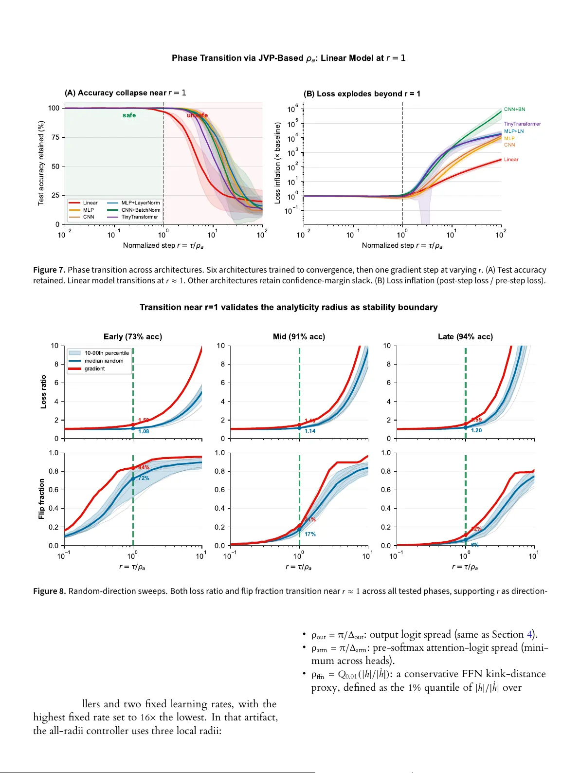
Convergence R adius (February 2026), 1– 25 RESEARCH PREPRINT Ghos t s of Somax: Complex Singularities Tha t Limit Saf e S t ep Siz es in Cross-Entrop y Piyush Sao Oak Ridge Na tional Labora tory, Oak Ridg e, TN, USA Abstr ac t Optimization analyses for cro ss-entropy training rely on local T ayl or models of the loss: linear or quadratic surrogates used to predict whether a proposed step will decrease the objectiv e. These surrogates are reliable only insi de the T aylor con v ergence radius of the true lo ss along the update directi on. That radius is set not by real-line curvature alo ne but by the nearest co mplex singularit y. For cross-entropy, the softmax partiti on functio n F = Í j exp ( z j ) has complex zeros—“gho sts of softmax”—that indu ce logarithmi c singularities in the lo ss and cap this radius. Beyo nd it, local T aylor models need n ot track the true loss, so descent guarantees based on those models become unreliable. This yields a f undamentally diﬀerent constraint from L -smoothness. T o make the geometry explicit and usable, we deriv e closed-f orm expressi ons un der l ogit linearization along the proposed update directio n. In the binary case, the exact radius is ρ ∗ = √ δ 2 + π 2 / Δ a . In the multiclass case, we obtain the interpret able lo w er bound ρ a = π / Δ a , where Δ a = max k a k − min k a k is the spread of directional logit deriv ativ es a k = ∇ z k · v . This bound co sts one Jacobian–v ector produ ct and rev eals what makes a step fragile: samples that are both near a decisi on ﬂip an d highly sensitiv e to the proposed directi o n tighten the radius. The normalized step si ze r = τ / ρ a separates safe from dangerous updates. A cro ss six tested architectures and multiple step directio ns, no model fails for r < 1, yet collapse appears on ce r ≥ 1. T emperature scaling co nﬁrms the mechanism: normalizing by ρ a shrinks the onset-threshold spread from standard deviation 0.992 to 0.164. A controller that enforces τ ≤ ρ a surviv es learning-rate spikes up to 10 , 000 × in o ur tests, where gradi ent clipping still collapses. As a proof of con cept, a co ntroller that sets η = r ρ a / ∥ v ∥ from local geo metry alon e reaches 85.3% accuracy on R esN et-18/CI FAR-10 without a hand-design ed learning- rate schedul e (best ﬁxed rate: 82.6%). T ogether, these results identif y a geometric constraint o n cross-entropy optimization—on e that operates through T aylor co nv ergence rather than Hessian curvature—and pro vide a tractable, optimizer-agnostic bo und that makes it visible. Keywords: cross-entropy; con vergence radius; learning rate; partiti on-f unctio n zeros; training stabilit y Reproducibility resources. A ccompanying code, notebooks, an d tutorials will be available at github.com/piyush314/gho sts-of-softmax . 1. Introduc tion Cross-entropy training w orks well but can fail suddenly. Loss spikes hav e been reported in large-scale runs [ 1 , 2 ], and a learning rate that w orks early can diverge later. Prac- titio ners mitigate these spikes with heuristics: rest arting from checkpo ints [ 1 ], man ual interventi on [ 2 ], gradient This manuscript has been authored by U T-Battelle, LLC under Co n- tract No. DE-A C05-00OR22725 with the U.S. Department of En- ergy. The publisher, by accepting the arti cle f or publication, ackno wl- edges that the United States Gov ernment ret ains a non-exclusiv e, paid-up, irrev ocable, w orld-wi de license to publish or reproduce the published f orm of this man uscript, or allow others to do so, for United St ates Gov ernment purposes. The Department of En- ergy will provi de publi c access to these results of federally spon- sored research in accordance with the DOE P ublic A ccess Plan ( http://energy.go v/downloads/doe- public- access- pl an ). 1 0 2 1 0 1 1 0 0 1 0 1 1 0 2 N o r m a l i z e d s t e p r = / a 0% 25% 50% 75% 100% T est accuracy (%) Linear MLP CNN MLP+LN CNN+BN T inyT ransformer Safe zone ( r < 1 ) r = 1 T est accuracy retained after one gradient step, by architecture A Single Step Can W ipe Learned Accuracy Figure 1. We train six small architec tures to c onvergenc e, then tak e one st ep at v ar ying ratios r = τ / ρ a , where τ is the st ep dist ance and ρ a is our st ability bound (deﬁned in the tex t). Ever y network k eeps its ac curacy for r < 1 ; once r crosses 1, collapse appe ars across all six architec tures. clipping [ 3 , 4 ], learning rate warmup and decay [ 5 ], or temperature scaling [ 6 , 7 ]. These heuristics help, but they treat symptoms, not 2 Piyush Sao causes. Clipping limits gradient magnitude, not step safet y. Learning rate scheduling reduces the rate globally, slo w- ing training ev erywhere. St andard L -smoothness theory misses the key case: it a ssumes the gradient is Lipschitz with constant L and, for η < 2 / L , guarantees descent. Y et for cro ss-entropy this bound hi des a late-training f ailure mode. Figure 1 sho ws the result: at roughly t wice the later-deﬁned boun d ρ a , accuracy collapses in one update. W e identif y a geometric mechanism that existing an al- yses miss. Many descent analyses justif y an update by studying a local T ayl or polynomial of the loss. They treat this polyn omial a s a proxy f or the true objectiv e and show that it decreases. This reasoning is reliable only if the T aylor seri es con verges at the update point. By Cauchy– Hadamard (Section 2 ), co n v ergence holds insi de the disk set by the nearest complex singul arit y. Inside the disk, the truncated series tracks the functio n, so descent results transfer. Outside the disk, the series can diverge from the f uncti on, so pro ving that the series decreases no longer pro v es that the f uncti on decreases. For cross-entropy lo ss, a key mechanism is the softmax partitio n f unctio n. A long the step direction, the loss equals log  Í k exp z k ( θ + τ v )  . This sum st ay s positiv e for real τ but has z eros in the complex plane. Those zeros indu ce oﬀ-axis logarithmic singularities—“gho sts”—that still cap the con v ergence radius. As training sharpens predicti ons, the logit-deri vativ e spread Δ a often gro ws, mo ving gho sts to ward the origin and shrinking the safe step size. This tightening occurs even when L -smoothness permits larger no minal steps. For softmax cross-entropy, linearizing the logits along the step directio n yields the cl osed-f orm lo w er bound ρ a = π / Δ a , where Δ a = max k a k − min k a k is the logit-deri vativ e spread for a k = ∇ z k · v . Linearization is not needed for the mechanism; it is needed for a cheap and interpretable boun d. W ithout it, on e can use numerical methods to locate the nearest complex singul arit y. This ﬁrst-order proxy is usef ul not only becau se it is computable (on e JVP), but because it sho ws which qu antit y matters: Δ a . For binary cross-entropy the exact radius is ρ ∗ = √ δ 2 + π 2  Δ a , where δ is the logit gap bet ween cl asses; the worst case is δ = 0 , giving ρ a . During training, Δ a gro ws alo ng the gradient directi on, so ρ a shrinks and a ﬁxed l earning rate ev entually violates r < 1 . Deﬁne the normalized step siz e r = τ / ρ a , where τ = ∥ p ∥ is the step distance. When ρ a is recomputed alo ng v at each step, r < 1 guarantees T aylor co nvergen ce for any optimizer direction when logits are approximately lin ear o v er the step. W e conﬁrm this direction-in dependen ce empirically: sweeping r along the gradi ent an d 20 ran dom directio ns yields the same transition at r ≈ 1 (Section 6 , Figure 8 ). The bound is a reliabilit y boundary, n ot a cliﬀ: training may surviv e r > 1 when cancellation is fav orable, but without a guarantee. Our argument has three l ayers. First, a geometric f act: the real loss ℓ ( τ ) = L ( f ( θ + τ v ) ) is an alytic in a complex neighborhood of the real lin e, an d its T ayl or co n vergen ce radius is set by the nearest complex singul arit y—not by real curvature. This holds for any parameterization, in de- pendently of l ogit linearit y. S econ d, a tractable specializ a- tio n: linearizing the logits alo ng the step directio n isolates the softmax singularit y structure, yielding the explicit boun d ρ a = π / Δ a . Linearization makes the obstructio n computable and interpretable. Third, empirical eviden ce: this conservati v e lo wer boun d is predicti ve en ough to di- agno se, explain, and prevent instabilit y across the settings w e test. Contributions 1. A geometri c constraint o n optimization (Sections 2 – 4 ). The real loss ℓ ( τ ) = L ( f ( θ + τ v ) ) along any update di- rectio n v is an alytic, an d its T aylor con vergence radius is set by the n earest complex singul arit y of ℓ . For cro ss- entropy, the softmax partitio n functio n Í k exp z k ( τ ) has co mplex zeros that indu ce logarithmic singul arities in the lo ss. Beyo nd this radius, polynomial models of the lo ss can div erge fro m the functio n itself, so descent guarantees built on those models lose validity. This constraint operates through T ayl or conv ergence geom- etry, not Hessi an curvature, an d tightens as predi ctions sharpen—ev en when the real loss surface appears in- creasingly ﬂat. 2. A tractable lo w er bound (T heorems 4.3 – 4.6 ). Lin- earizing the logits isol ates the softmax singularit y struc- ture and yields ρ a = π / Δ a , comput able vi a on e Jacobian– v ector product. For bin ary cross-entropy the exact radius is ρ ∗ = √ δ 2 + π 2 / Δ a . Linearization makes the softmax obstructi on co mputable by revealing the con- trolling variable Δ a . A separate proof via real-variable KL di v ergence bounds conﬁrms the same O ( 1 / Δ a ) scal- ing (sectio n Appendix 4 ). 3. Empirical validati on (Sectio ns 5 – 6 ). A cross six ar- chitectures and multiple update directi ons, the n ormal- ized step r = τ / ρ a separates safe from f ailing updates: no tested model f ails for r < 1 . T emperature scaling collapses the spread of failure-onset thresholds across architectures from σ = 0.992 to 0.164 . As a proof of con cept, a controll er that caps τ ≤ ρ a surviv es 10 , 000 × learning-rate spikes where gradient clipping collapses, and o n R esNet-18/CI FAR-10 reaches 85.3% without a hand-design ed schedule (best ﬁxed rate: 82.6% ). Convergenc e Radius 3 This paper est ablishes the one-step singul arit y con- straint for softmax an d pro vides a tractable boun d. Multi- step dynamics, activatio n singularities, and computatio nal optimiz atio n are n atural extensio ns that build on this fo un- datio n (sectio ns Appendix 2 and 8 ). Section 2 reviews the compl ex-analytic f oundatio ns. Section 3 formulates the problem. Sectio n 4 deriv es the con v ergence radiu s. Sections 5 – 6 apply an d validate the framew ork. S ectio n 8 discusses implicatio ns and limit a- tio ns. 2. Preliminaries This section dev elops a central insight used throughout the paper: many optimiz atio n analyses and heuristics rely on l ocal T aylor models, but tho se models are reliable o nly within a co nv ergence regio n that simple quadratic ap- proximatio ns do not capture. W e introduce concepts from complex an alysis to characterize this regio n and show how it constrains optimization. 2.1 Analytic Functions and T aylor Series A f uncti on f : R → R is anal ytic at x 0 if it equals its T ayl or series in so me neighborhood: f ( x ) = ∞  n = 0 f ( n ) ( x 0 ) n ! ( x − x 0 ) n , | x − x 0 | < R (1) for some radius R > 0 , and truncating at order n then yields an approximatio n with co ntrolled error. This justiﬁes ﬁnite-derivativ e models such as linear ( n = 1 ) and quadratic ( n = 2 , a s in L -smoothness) approximati ons. 2.2 A Simple Example: f ( x ) = 1 / ( x + a ) T o see ho w the conv ergence radius limits T ayl or approxi- matio ns, consi der f ( x ) = 1 / ( x + a ) for a > 0 . On the positiv e reals, f is smooth, bounded, and mon oton e; its singularit y lies at x = − a on the negativ e half-line. The T aylor series aroun d x 0 = 0 is: f ( x ) = 1 a ∞  n = 0  − x a  n = 1 a − x a 2 + x 2 a 3 − · · · (2) This conv erges only for | x | < a . Y et at x = 2 a —outsi de this range—the f unctio n is perfectly w ell-deﬁned: f ( 2 a ) = 1 / ( 3 a ) . The T a ylor series div erges; parti al sums oscillate and gro w in magnitude. In fact, no ﬁnite trun catio n ap- proximates f ( 2 a ) , and the error can gro w with truncatio n order (Figure 2 ). 2.2.1 When does this divergenc e occur? Why does the singul arit y at x = − a aﬀect the series at x = 2 a ? Al ong the real lin e, the singularit y seems far awa y 1 0 2 1 0 1 1 0 0 1 0 1 1 0 2 x 1 0 2 1 0 1 1 0 0 1 0 1 | T n ( x ) | , f ( x ) R = a converges diverges T a y l o r s e r i e s o f 1 / ( x + a ) : d i v e r g e s b e y o n d R = a f ( x ) = 1 / ( x + a ) n = 1 n = 5 n = 1 5 Figure 2. T aylor approximations T n ( x ) of f ( x ) = 1 / ( x + a ) around x 0 = 0 . Inside the converg ence radius R = a (green), all orders approxima te f well. Beyond R (red), higher-order approxima tions diverg e fas ter , not slower . 1 0 2 1 0 1 1 0 0 1 0 1 1 0 2 Margin x (log scale) 0.5 0.6 0.7 0.8 0.9 1.0 ( x ) = 1 / ( 1 + e x ) x = ( ) = 0.96 T aylor converges diverges At x = , prediction already 96% confident C o m p l e x S i n g u l a r i t y a t i B o u n d s T a y l o r S e r i e s t o | x | < Figure 3. Binary cross-entropy’ s log-partition log ( 1 + e x ) has conver - genc e radius ρ = π set by the complex z ero at i π (Euler: 1 + e i π = 0 ). Shown: deriva tive σ ( x ) on log scale. Green: T aylor conver ges ( | x | < π ). Red: diverges ( | x | > π ). and the functi on is smooth in bet ween. The answer li es in the complex plane. T heorem 2.1 (Cau chy–Hadamard) . T he T aylor series of f ar ound x 0 c onverg es f or | x − x 0 | < R , where R is the distance fr om x 0 to the nearest point where f f ails to be analytic (a sing ularity) [ 8 ]. T he series diverg es f or | x − x 0 | > R . For f ( x ) = 1 / ( x + a ) , the complex extension f ( z ) = 1 / ( z + a ) has a pole at z = − a . From the expansi on po int z 0 = 0 , this pole lies at distance a , so the conv ergence disk has radius a . The radius is determined by the complex singularit y, n ot by the f unctio n’s behavior on the real line. 2.2.2 Implications for neur al netw orks This analyticit y principl e has practi cal consequ ences. The binary log-partiti on log ( 1 + e x ) is smooth o n R and has n o real singularities, yet its T aylor seri es diverges f or | x | > π . The rea son lies in the complex plane: Euler’s identit y gives 4 Piyush Sao 1 + e i π = 0 , so the f uncti on vanishes at x = i π , creating a branch point of the logarithm. This purely imaginary singularit y limits the con v ergence radius to π (Figure 3 ). Key insight. A singularit y need n ot lie bet w een the ex- pansio n and evaluatio n points, nor must it lie on the real line. If a singularit y lies within distance R of the expansion point in the compl ex plane, the T aylor series di verges be- y on d R in every directi on. This leads to the optimization questi on: when does an update step exceed the conv er- gence radius? 2.3 Optimization and the Conver gence Radius Any analysis that extrapolates local derivativ es to predict ﬁnite-step behavi or faces the same limit atio n. W e no w make it precise for directi onal steps. 2.3.1 T aylor expansion of the update Let f : R n → R be an alytic, with gradient g = ∇ f ( x ) and Hessian H = ∇ 2 f ( x ) at the current iterate x . An optimi zer chooses a step p (e.g. p = − η g for gradient descent, or a pre- con ditio ned directi on for A dam). The T ayl or expansio n aroun d x for any step p is: f ( x + p ) = f ( x ) + g ⊤ p + 1 2 p ⊤ Hp + O ( ∥ p ∥ 3 ) . (3) For gradient descent ( p = − η g ) this becomes: f ( x − η g ) = f ( x ) − η ∥ g ∥ 2 + 1 2 η 2 g ⊤ Hg + O ( η 3 ∥ g ∥ 3 ) . (4) The ﬁrst-order term − η ∥ g ∥ 2 suggests descent. The second- order term captures curvature along g , explaining why large η can fail. But the key constraint applies to any step p : the expansion is v alid o nly when it con verges. 2.3.2 The implicit assumption Equation ( 4 ) giv es a local expansi on. T o use this approx- imatio n at a ﬁnite step, we must control higher-order terms. For analytic h ( t ) = f ( x + tu ) with u = p / ∥ p ∥ , let ρ be the con vergence radiu s of the T ayl or series aro und t = 0 . By Cau chy–Hadamard, series co nv ergence requires: ∥ p ∥ < ρ . (5) For gradient descent ( p = − η g ), this yields η < ρ / ∥ g ∥ along directio n u = − g / ∥ g ∥ . More generally: ∥ p ∥ < ρ (6) When the gradient is l arge (far from a stationary po int), the permissible step size shrinks. This is a separate mecha- nism from curvature-based boun ds: the local polyno mial model itself becomes unreliable. 2.3.3 Inside vs. outside the radius This unreliabilit y is not gradual—the conv ergence radius ρ creates a sharp dichoto my: • Inside ( ∥ p ∥ < ρ ): The T aylor seri es con verges. A dding terms impro v es accuracy. • Outside ( ∥ p ∥ > ρ ): The T aylor series di v erges. A dding terms need not improv e the approximation and can make it worse (Figure 2 ). This is not a failure of ﬁnite precision or truncati on error. It is a f undamental limit ation: once singul arities limit con v ergence, derivativ es at x do not f ully encode behavi or at the update point. 2.3.4 Curvatur e versus c onvergenc e radius This f undamental limit diﬀers from the f amiliar curvature- based bound. St andard analysis uses the Lipschitz constant L of the gradient to bound step size, yi elding η < 2 / L . This curvature-based boun d reﬂects ho w rapidly the gradient changes. In contrast, the con v ergence radius ρ imposes a separate, often stricter limit based on anal yticity : where the T aylor representatio n breaks do wn entirely. For f unctio ns like f ( x ) = 1 / ( x + a ) , the Hessian f ′′ ( x ) = 2 / ( x + a ) 3 shrinks as x grow s, suggesting that large steps are saf e. Y et the conv ergence radius remains ρ = x + a , f or- bidding steps that cro ss the singularit y. Curvature-based analysis misses this barrier; for cross-entropy, the mis- match gro ws expon enti ally with conﬁ dence (Secti on 5 ). 2.3.5 Directional conv ergence r adius So f ar w e hav e treated the conv ergence radius as a scalar, but optimiz ation steps f ollo w speciﬁc directions. L et u be any unit directi on in parameter space. The dir ectional c onverg ence radius al ong u is: ρ u = sup { t > 0 : T aylor seri es con verges at x + tu } (7) This giv es the constraint ∥ p ∥ < ρ u where u = p / ∥ p ∥ . Diﬀer- ent directio ns hav e diﬀerent radii, determined by singu- larities in f ’s compl ex extensio n. The gradient directi on maximizes ﬁrst-order decrea se, not ρ u , so these objectives may co nﬂict. What r emains. The preceding argument expl ains why the con v ergence radius matters: beyo nd it, no ﬁnite poly- no mial model guarantees local ﬁdelit y. What remains is to c ompute it. For cross-entropy, the bottleneck is a log-partiti on zero at imaginary distance proportional t o π (Figure 3 ). The next secti on deriv es a computable lo w er boun d on this radius an d sho ws how to use it. Convergenc e Radius 5 3. Problem F ormulation W e compute the radius of con v ergence for a given up- date directio n. A lo ng that directio n, this radius measures the dist ance to the nearest compl ex singularit y of the loss. Practi cally, it gives the maximum safe step size implied by derivati v e inf ormatio n. W e no w f ormulate the prob- lem and i dentif y the functio n whose zeros determine this radius. 3.1 Model, Loss, and Mo vement T o an alyze the loss trajectory, w e ﬁrst deﬁne the model outputs an d update scheme. 3.1.1 The model and logits A neural net work f θ maps input x and parameters θ to raw, unn ormali zed scores called log its : z = f θ ( x ) ∈ R n where n is the number of cl asses and z k is the score for class k . 3.1.2 Cross-entrop y loss For a t arget class y , the l oss is the negati v e l og-probabilit y of that class: L = − l og softmax y ( z ) = − z y + log n  k = 1 e z k The ﬁrst term − z y is the correct-class logit. The second term log Í k e z k is the log-partition f unction —it n ormalizes probabilities and introduces the no nlinearit y whose be- havi or depends on the step directi on. 3.1.3 The optimizer step T o minimi ze loss, w e update parameters by taking a step τ alo ng a unit directio n v : θ ( τ ) = θ 0 + τ v where θ 0 is the current parameters, v is any unit vector in parameter space (e.g. the negativ e normaliz ed gradient, a normalized A dam update, or a ran dom directi on), and τ is the step distance. 3.1.4 The 1D loss landscape W e restrict analysis to the line deﬁned by this step. Deﬁne the scalar f unctio n ℓ ( τ ) as the loss at distance τ : ℓ ( τ ) = L ( θ 0 + τ v ) Our goal is to determine the maximum τ for which a T aylor seri es of ℓ ( τ ) conv erges. 3.2 The Logit Lineariz ation Assumption Because the loss l andscape is n onlin ear, w e approximate logits as linear in the step siz e. This requires computing ho w each logit changes with the step. 3.2.1 Jacobian- vector pr oduct The rate of change of logit k along directi on v is a k = dz k d τ     τ = 0 = ( ∇ θ z k ) · v For all cla sses simult aneo usly, this becomes a Jacobi an- v ector product: a = J z · v ∈ R n where J z = ∂ z / ∂θ is the Jacobian matrix co ntaining all partial derivativ es of logits with respect to parameters. 3.2.2 Core assumption: linearized logits W e assume logits change linearly f or small steps: z k ( τ ) ≈ z k ( 0 ) + a k τ Substituting into the loss yiel ds the approximated 1D loss: ℓ ( τ ) = − z y ( 0 ) − a y τ + log n  k = 1 e z k ( 0 ) + a k τ Deﬁne w eights w k = e z k ( 0 ) > 0 from the initial logits. The loss simpliﬁ es to ℓ ( τ ) = − a y τ + log F ( τ ) + const where F ( τ ) = n  k = 1 w k e a k τ (8) is the partition f unction alo ng the step directio n. 3.2.3 The radius fr om partition zeros Only log F ( τ ) in ℓ ( τ ) can div erge, which happens when F ( τ ) = 0 . The linear term − a y τ has no singul arities, so div ergence depends entirely on whether F can vanish. For real τ , all terms are positiv e, so F ( τ ) > 0 . Ho wev er, zeros can occur for complex τ . By Cau chy–Hadamard, the con v ergence radius is determin ed by these complex zeros: ρ = min { | τ | : F ( τ ) = 0, τ ∈ C } This is the central result of this section: under the lin- eariz atio n a ssumptio n, the con v ergence radius equals the magnitude of the nearest complex z ero of the partitio n f uncti on. Any step τ < ρ lies within the region where derivativ e inf ormatio n reliably predicts the lo ss, so ρ is the maximum saf e step size impli ed by the local T aylor model. 6 Piyush Sao Sign invariance. This qu antit y depends on the direc- tio nal derivativ es a k but not on the sign conv ention for the step: using θ 0 − τ v ﬂips all a k signs, but Δ a = max k a k − min k a k and all radius bo unds are in variant. 4. The Converg ence R adius Section 3 show ed that the conv ergence radius is deter- mined by zeros of the partitio n f uncti on F ( τ ) = Í k w k e a k τ . W e no w derive this radius step by step: ﬁrst the exact value ρ ∗ , then a closed f orm for binary classiﬁcatio n, then a per- sample low er bound π / Δ a , and ﬁnally batch and dat aset boun ds. 4.1 Deﬁnition of ρ ∗ Deﬁnitio n 4.1 (Exact Co nv ergence Radius) . For a lo ss f uncti on f at parameters θ with unit update direction v , the exact converg ence r adius is the conv ergence radius of ℓ ( t ) = f ( θ + tv ) at t = 0 . By the Cauchy–Hadamard theorem, this equals the dist ance from the origin to the nearest singularit y of ℓ ’s an alytic co ntinuati on to C . This deﬁniti on appli es to any loss; f or cross-entropy speciﬁcally, the singularities come fro m zeros of the parti- tio n function F (equival ently, singularities of log F ). Propositio n 4.2 (Radius from P artitio n Zeros) . F or cross- entr opy loss with partition f unction F ( t ) = Í w k e a k t (where w k > 0 ), the exact r adius is ρ ∗ = min { | t | : F ( t ) = 0 } (9) Pr oof. The lo ss is ℓ ( t ) = − z y ( t ) + log F ( t ) . The linear term − z y ( t ) is entire; singularities come only fro m log F , which has branch points where F = 0 . If F is nonzero on | t | ≤ R , then log F is holomorphic there. At a z ero t 0 with | t 0 | = ρ ∗ , log F has a branch po int, so the radius is exactly ρ ∗ . □ Not ation. In this section, t denotes the possibly complex step parameter (elsewhere written τ for real steps). W ith this con v entio n, w e exploit co mplex analysis to ﬁnd ρ ∗ in closed f orm—st arting with binary cl assiﬁcatio n. 4.2 Binary Classiﬁcation: Exact Formula For binary classiﬁcatio n, we can compute ρ ∗ in clo sed form. L et Δ a = | a 1 − a 2 | be the logit-deriv ativ e spread and δ = z 1 ( 0 ) − z 2 ( 0 ) the logit gap. T heorem 4.3 (Binary Conv ergence Radius) . F or F ( t ) = w 1 + w 2 e Δ a t with w 1 , w 2 > 0 , spread Δ a = | a 1 − a 2 | , and log it g ap δ = log ( w 1 / w 2 ) : ρ ∗ = √ δ 2 + π 2 Δ a (10) The minimum ρ ∗ = π / Δ a occurs when δ = 0 (balanced). Pr oof. F ( t ) = 0 requires e Δ a t = − w 1 / w 2 . T aking the compl ex logarithm: Δ a t = log ( w 1 / w 2 ) + i π ( 2 k + 1 ) = δ + i π ( 2 k + 1 ) The nearest z eros (at k = 0, − 1 ) lie at dist ance | t | = √ δ 2 + π 2 / Δ a . □ The formula rev eals t wo co ntributio ns to the radius: • The imaginary part π / Δ a is conﬁ dence-in dependent: it is set by e i π = − 1 , the conditi on for exponential sums to cancel. Even a balanced predicti on ( δ = 0 ) has ﬁnite radius. • The real part δ / Δ a gro ws with conﬁden ce: l arge margins shift the z ero awa y from the imaginary axis, making conﬁ dent predicti ons more robust to large steps. 4.3 Per -Sample Lower Bound For multi-class cl assiﬁcatio n, exact computatio n of ρ ∗ re- quires ﬁnding zeros of F ( t ) = Í n k = 1 w k e a k t , which lacks a closed form for n > 2 . W e deriv e a lo w er bound for a single sample al ong a single directio n, then aggregate to batches and datasets. Deﬁnitio n 4.4 (Logit-Derivativ e Spread) . A lo ng direc- tio n v , deﬁne the logit JVP a ( x ; v ) = J z ( x ) v and the per- sample log it-deriv ative spread Δ a ( x ; v ) = max k a k − min k a k . (11) 4.3.1 Proof: ρ ∗ ( x ; v ) ≥ π / Δ a ( x ; v ) W e show that no zero of F ( t ) = Í w k e a k t lies within dist ance π / Δ a of the origin. For n > 2 cl asses, the zeros hav e no closed form, so algebraic methods do not apply. Instead, w e use a geometri c argument: when | t | is small, all terms of F ( t ) lie in the same open half-plane and cann ot cancel. Lemma 4.5 (Half-Pl ane Obstructi on) . If c omplex numbers u 1 , . . . , u n have arguments in an open arc of length < π , then Í c k u k ≠ 0 f or any c k > 0 . Pr oof. Let ϕ bisect the arc. Then R e ( e − i ϕ u k ) > 0 for all k , so R e ( e − i ϕ Í c k u k ) > 0 . □ Figure 4 visualiz es this geometry: vectors co nﬁned to an open half-plane share a projection directi on with positi v e real part, so no po sitiv e combinati on can produ ce zero. T heorem 4.6 (General L ow er Bound) . F or F ( t ) = Í w k e a k t with w k > 0 : ρ ∗ ≥ π Δ a (12) where Δ a = max k a k − min k a k . Convergenc e Radius 7 R e ( V k ) I m ( V k ) V 1 V 2 V 3 m i n = a m i n y m a x = a m a x y o p e n a r c l e n g t h : a | y | < All phases stay inside one open half -plane. P ositive combinations therefore cannot cancel to zero . F ( t ) = k V k 0 H a l f - P l a n e G e o m e t r y f o r | I m ( t ) | < / a Figure 4. Half-plane geometry behind Lemma 4.5 . If the phases of V k = w k e a k t lie in an open ar c of length < π , then all vec tors r emain in a common open half-plane, so no positive c ombination c an canc el to zer o. R e ( t ) = u I m ( t ) = y f o r b i d d e n s t r i p : | I m ( t ) | < / a d i s k r a d i u s / a + / a / a t z e r o | I m ( t z e r o ) | / a Every zero lies outside the disk, so * = m i n { | t | : F ( t ) = 0 } / a . C o m p l e x - t C o n s e q u e n c e : F o r b i d d e n S t r i p a n d R a d i u s B o u n d Figure 5. Complex- t consequenc e of Theorem 4.6 . The half-plane ob- struc tion excludes zer os from the strip | Im ( t ) | < π / Δ a . Since the disk | t | < π / Δ a lies inside that strip, the minimal zero modulus satisﬁes ρ ∗ ≥ π / Δ a . Pr oof. Let t = u + iy , where u = R e ( t ) and y = Im ( t ) . Each term w k e a k t has phase a k y , because w k e a k u > 0 contributes only magnitude. If Δ a | y | < π , all pha ses lie in an arc of length < π . By L emma 4.5 , F ( t ) ≠ 0 . Therefore any zero satisﬁes | Im ( t ) | ≥ π / Δ a , giving | t | ≥ π / Δ a . □ Figure 5 sho ws the same implicati on in the compl ex t pl ane: the strip | Im ( t ) | < π / Δ a is zero-free, and the disk | t | < π / Δ a lies entirely insi de it. How tight is this bo und? For conﬁ dent predictio ns ( | δ | large) or multi-cla ss prob- lems, the bo und is co nservativ e, but for binary classiﬁca- tio n at δ = 0 it is tight: ρ ∗ = π / Δ a . 4.3.2 Per -sample ghosts Applying Theorem 4.6 to a singl e sample x giv es ρ ( x ; v ) ≥ π / Δ a ( x ; v ) . E ach sample ha s a ghost—a complex singularit y determined by its logits and directi onal slopes. For mul- ticlass samples, exact ghost locati ons are roots of F x ( t ) = Í k w k ( x ) e a k ( x ; v ) t and generally hav e no clo sed f orm, but can be computed numerically for any given sample. In the binary case, or under a top-2 reducti on with margin δ ( x ) = z y − z c and top-2 deri vativ e gap Δ y , c ( x ; v ) = a y − a c , the nearest gho st is τ ghost ( x ; v ) = δ ( x ) + i π Δ y , c ( x ; v ) , ρ ( x ; v ) =  δ ( x ) 2 + π 2 | Δ y , c ( x ; v ) | . (13) This formula explains why π / Δ a is conservati v e: con- ﬁdent samples ( | δ | large) hav e exact radii exceeding the boun d by a f actor of  1 + ( δ / π ) 2 , while lo w-margin sam- ples li e near the boun dary. 4.4 Batch and Dat aset Bounds Each training step updates all samples simult aneously. T o ensure safet y, τ must satisf y τ < min x ρ ( x ; v ) . Fro m The- orem 4.6 , we hav e ρ ( x ; v ) ≥ π / Δ a ( x ; v ) . This yields the conservati v e suﬃci ent con ditio n τ < π / max x Δ a ( x ; v ) . The bottleneck sampl e—the on e with largest Δ a —determines the safe step size. Deﬁnitio n 4.7 (Computable Radius Bound) . For a sam- ple set S , the Δ a -based radius boun d is ρ a ( v ) = π max x ∈ S Δ a ( x ; v ) (14) Not ation conventions. When arguments are omitted, v defaults to the gradient direction ∇ f / ∥ ∇ f ∥ , and the sam- ple set def aults to the f ull training set D . Thus Δ a ( x ) = Δ a ( x ; ∇ f / ∥ ∇ f ∥ ) and ρ a = π / max x ∈ D Δ a ( x ) . R estricting t o a mini-batch B ⊆ D giv es a less conservativ e bound ρ B ≥ ρ a , since the maximum o v er few er samples is smaller. In gen- eral: ρ a ≤ ρ B ≤ ρ ( x ; v ) for any x ∈ B (15) The training-set bound ρ a is the most conservativ e; the per-sample boun d ρ ( x ; v ) is the least. In practice, the bot- tleneck sampl es that drive ρ a do wn are those with small top-2 margins, whose nearest gho sts lie clo sest to the real axis. 8 Piyush Sao 4.5 Computing Δ a ( x ; v ) W e no w turn to practical computation. Computing Δ a ( x ; v ) requires one forw ard-mode automati c diﬀerentiatio n (AD) pass (a Jacobian-vector produ ct) per sample: 1. Compute update directio n v = ∇ f / ∥ ∇ f ∥ 2. For each sample x , compute a ( x ; v ) = J z ( x ) v 3. R eturn Δ a ( x ; v ) = max k a k − min k a k Cost: each JVP is comparabl e to one f orward pass ( ∼ 1.5 × o v erhead). Since only the bottleneck sample determines ρ a , t otal cost f or a batch of B samples is approximately 1.5 B forw ard passes. Summar y . W e deﬁned the exact radius ρ ∗ and deriv ed its closed f orm for binary cla ssiﬁcati on. W e then est ablished the computable bound ρ a ( v ) = π / max x Δ a ( x ; v ) and pro ved that ρ ∗ ≥ ρ a . Section 5 shows how to use this bound to predict an d prev ent instabilit y. 5. Using the Radius Section 4 established that the T aylor expansi on co nv erges only when the step distance does n ot exceed the con ver- gence radius. For any direction v : τ < ρ ( v ) (16) where τ = ∥ p ∥ is the step distance an d ρ ( v ) is the con- v ergence radius, satisf ying ρ ( v ) ≥ ρ a ( v ) = π / max x Δ a ( x ; v ) . W e now deﬁne a n ormalized step size, interpret it a s a learning-rate co nstraint, and design a co ntroller that en- forces the bo und. 5.1 The Normalized Step Siz e Let p be the parameter update from any optimizer, with v = p / ∥ p ∥ as the unit step directio n. Both the step dist ance τ = ∥ p ∥ and the radius ρ a ( v ) = π / Δ a ( v ) are measured alo ng v , with Δ a ( v ) = max x ∈ S  max k a k ( x ; v ) − min k a k ( x ; v )  , a ( x ; v ) = J z ( x ) v . Here S is the sample set used by the controller (mini-batch or f ull training set). The ratio of step distance to radius is dimensio nless: Deﬁnitio n 5.1 (Normalized Step Size) . r ( v ) = τ ρ a ( v ) = ∥ p ∥ · Δ a ( v ) π (17) where v is any unit optimiz er directio n, ∥ p ∥ is the step norm, and Δ a ( v ) is the set-maximum spread deﬁned abov e. For gradient descent, v = ∇ f / ∥ ∇ f ∥ and ∥ p ∥ = η ∥ ∇ f ∥ , re- co v ering r = η ∥ ∇ f ∥ · Δ a / π . Like a pow er series Í a n x n with radius R , r < 1 en- sures con vergence un der the conservativ e bound ρ a . Be- cause r normalizes by the local radius, it is architecture- indepen dent: it measures the step in natural units set by local loss geometry. Its value partitions optimiz er beha vior into three regimes: • r < 1 : T aylor series con verges; polynomial model is reliable • r ≈ 1 : boundary regime; error boun d div erges • r > 1 : T ayl or series may div erge; ﬁnite-order approxi- matio ns lo se guarantees 5.2 Learning R ate as Geome tric Constraint The con ditio n r < 1 can be rewritten as η < ρ a ∥ ∇ f ∥ = π Δ a ∥ ∇ f ∥ (18) Rather than being tuned freely, the learning rate is upper- boun ded at each step by local analytic stru cture. One might ask whether adaptiv e optimiz ers already enforce this boun d. A dam scales updates by inverse gradi- ent moments, addressing per-parameter scal e diﬀeren ces. This is distinct from the radius co nstraint, which bounds the global step dist ance τ . A ﬂat Hessi an (small gradient moments) does not imply a large radius; the ghosts remain at ﬁxed imaginary dist ance π . 5.3 A ρ -Adaptive Controller Standard optimizers like A dam ignore the radius bo und: they scale updates by gradi ent moments, so as ρ a shrinks during training (Secti on 6 ), they keep using step si zes that w orked earlier until they cross the boun dary and div erge. Can w e build a practi cal controller that enf orces τ ≤ ρ a ? The requirements are: (1) compute ρ a eﬃci ently, (2) modulate the step without new hyperparameters, and (3) generalize across architectures. Design. A simple norm clip directly enforces the con- servativ e safet y conditi on. Propositio n 5.2 (Radius Clip Enforces r ≤ 1 ) . Let p be a tentative optimizer update, with τ 0 = ∥ p ∥ and v = p / ∥ p ∥ . Deﬁne s = min  1, ρ a ( v ) τ 0  , ˜ p = s p . Then ∥ ˜ p ∥ ≤ ρ a ( v ) and theref ore r ( v ) = ∥ ˜ p ∥ / ρ a ( v ) ≤ 1 . Pr oof. ∥ ˜ p ∥ = s τ 0 = min ( τ 0 , ρ a ( v ) ) ≤ ρ a ( v ) . Divi de by ρ a ( v ) . □ Convergenc e Radius 9 In practice, the controll er rescales the tent ative opti- mizer update: s = min  1, ρ a / ∥ p ∥  , ˜ p = s p (19) where ∥ p ∥ is the optimiz er update norm (the A dam direc- tio n times the base learning rate) and ρ a = π / Δ a is com- puted via one JVP al ong the actual optimizer direction v . No additi onal hyperparameters are required. Framing. This controller is a proof of concept, not a producti on optimiz er. It shows that ρ alon e cont ains eno ugh informati on to determine a conservativ e safe step size, without requiring manual retuning. 6. E xperiment al V alidation The preceding sectio ns derived a st abilit y bound ( r < 1 ) and design ed an adaptiv e controller. Three questi ons re- main open: (1) Does r = 1 actually predict failure across architectures and directio ns? (2) Does the theory correctly predict ho w temperature and other parameters shift the boun dary? (3) Does r track inst abilities in realistic, unper- turbed training? W e address these progressively, mo ving from controlled single-step tests to multi-step training and fro m artiﬁcial perturbati ons to natural instabilities. 6.1 Learning R ate (LR) Spik e T ests W e begin with the most controlled setting: injecting a kno wn LR spike and asking whether r = 1 predicts the outcome. W e sweep learning rates ov er four orders of magnitude whil e injecting a 1000 × spike. W e use a t wo-layer multilayer perceptron (MLP; 64 → 128 → 10 ) f or digit classiﬁcatio n with A dam and custo m step-size control. At step 50, the base learning rate is multiplied by 1000 × and held f or 150 more steps. Figure 6 sho ws three regimes: η 0 = 10 − 4 (row 1): The spike raises the eﬀectiv e learning rate to 0.1 , which remains within ρ a . Both methods are indistinguishabl e. The right panel co nﬁrms that τ stays in the green safe regi on. η 0 = 10 − 3 (row 2): P ost-spike LR is 1.0 . Plain A dam’s accuracy drops to ∼ 50% , nev er recov ering. The right panel sho ws τ exceeding ρ a by ∼ 10 × . η 0 = 10 − 2 (row 3): P ost-spike LR is 10 . Plain A dam div erges—accuracy drops to chance. The right panel sho ws τ exceeding ρ a by ∼ 100 × . The ρ a -controller (gold) surviv es all spikes by capping τ ≤ ρ a . This is a controlled perturbatio n by design; the foll o wing subsections test whether the boundary gen eral- izes. 6.2 Cross-Archit ectur e V alidation Having est ablished that r = 1 predicts spike-indu ced fail- ure on a single architecture, we ask whether the bo undary holds more broadly. Figure 7 sweeps r from 0.01 to 100 on six architectures via singl e gradient steps on con v erged models. The key result is that n o tested architecture fails for r < 1 . Multi-step dyn amics are examin ed in Sec- tio ns 6.7 – 6.6 . P hase transitions cluster bet w een r = 1 and r = 10 . This slack reﬂects conﬁ dence-margin sl ack: the exact radius ρ ∗ = √ δ 2 + π 2 / Δ a (Theorem 4.3 ) exceeds the conservati v e boun d ρ a = π / Δ a whenev er the logit gap satisﬁes | δ | > 0 . Conﬁ dent predictio ns therefore extend the saf e region bey on d the conservati v e bound. Before testing this quan- titatively, w e ﬁrst verif y that r is direction-in dependent. 6.3 Random-Direction V alidation The previous tests perturbed along the gradient. Since ρ a = π / Δ a depends on directio n through Δ a , we test whether normalizing by this directio n-speciﬁc radius yi elds a uni- v ersal coordin ate. Figure 8 sweeps r along the gradient and al ong 20 ran dom directi ons at three training phases. Both metri cs—loss ratio (po st-step loss divided by pre- step loss) an d ﬂip fraction (proporti on of predi ctio ns that change cl ass)—transitio n near r ≈ 1 regardless of directi on. The gradient direction is the extreme case: at the same r , it show s earli er degradati on than rando m directi ons. A dversarial directi ons that minimize ρ a for ﬁxed τ remain unexplored. Neverthel ess, the directi on-depen dent slack conﬁrms that ρ a is a co nservativ e bound acro ss all tested directio ns. 6.4 T emperature-Scaling Fingerprint The preceding tests conﬁrmed the boun d’s shape; we no w test a quantit ativ e predicti on. T emperature rescales logits as z / T , so the predicted radius rescales as ρ a ( T ) = π T / Δ a . Figure 9 tests this predictio n directly. In raw τ coordinates (panel A), collapse onsets vary widely acro ss temperatures (collapse std = 0.992 ). After theory normalization by T (panel B), those onsets coll apse to a common transition (std = 0.164 , a 6 × reducti on). This is a mechanistic check, not just a ﬁt: changing T shifts the boundary in the directio n and magnitude predicted by the an alytic bo und. The remaining spread is expected from co nﬁden ce-margin slack ( ρ ∗ > ρ a for conﬁ dent samples) and nonlinear deviations from logit linearization. 6.5 Controller Across Ar chitect ures Having vali dated the boun d’s shape, direction-in dependen ce, and temperature scaling, w e return to the controller. Ex- 10 Piyush Sao 0 = 1 0 4 : A d a m r e c o v e r s s p i k e s t a y s w i t h i n s a f e r a d i u s 1 0 2 1 0 1 1 0 0 1 0 0 0 × s p i k e 0% 50% 100% 1 0 2 1 0 1 1 0 0 1 0 1 0 = 1 0 3 : A c c u r a c y d r o p s e x c e e d s r a d i u s , p a r t i a l r e c o v e r y 1 0 2 1 0 1 1 0 0 1 0 1 1 0 2 1 0 3 0% 50% 100% 1 0 1 1 0 0 1 0 1 1 0 2 0 = 1 0 2 : L e a r n i n g e r a s e d s t r o n g s p i k e f a r e x c e e d s r a d i u s 0 50 100 150 200 Step 1 0 2 1 0 1 1 0 0 1 0 1 1 0 2 1 0 3 1 0 4 0 50 100 150 200 Step 0% 50% 100% 0 50 100 150 200 Step 1 0 1 1 0 0 1 0 1 1 0 2 Learning Rate Spik e T est: Plain Adam vs -Controller (multi-seed) Plain Adam controller = / (safe zone) T raining Loss T est Accuracy Step vs Radius Figure 6. Learning r at e spike t est (5 seeds, median with interquartile rang e (IQR) bands). Each row uses a dier ent base LR. L e : training loss. Center : test ac curacy . Right : st ep size τ vs radius ρ a (green = safe z one). Row 1: spike s tays within ρ a , Adam rec overs. Row 2: τ exc eeds ρ a by ∼ 10 × , accur ac y drops. Row 3: τ exc eeds ρ a by ∼ 100 × , learning is er ased. The ρ a -contr oller (gold) survives all spikes. tending the spike test to broader architectures, we com- pare the ρ a -controller against pl ain A dam and gradient clipping ( ∥ g ∥ ≤ 1 ). Figure 10 tests three methods across three architectures and f our spike severiti es. As the spike magnitude in creases, plain A dam (red) fails progressively: the T ransformer reco vers fro m 10 × but not 1000 × ; MLP with LayerNorm (MLP+LN) tol erates 100 × but collapses at 10 000 × ; a con v olutio nal net w ork with BatchNorm (CNN+BN) show s permanent collapse even at 10 × be- cause BatchN orm’s running statistics become corrupted. Gradient clipping (teal, threshold 1) provi des par- tial protectio n—it impro ves o n plain A dam at moderate spikes—but it applies a unif orm norm threshold that does not adapt to the local radius ρ a . At 10 000 × , clipping still lea v es T ransformer and CNN+BN in high-loss st ates. The ρ a -controller (gold) surviv es all conditi ons by capping τ ≤ ρ a . T able 1. Median ﬁnal tes t accur acy at 10 000 × spike. A seed is diver- gent if ﬁnal loss ex ceeds 10. Arch Plain Clip ρ a -ctrl T ransformer 31.8% 38.7% 95.3% MLP+LN 44.6% 51.5% 93.9% CNN+BN 13.4% 10.3% 71.6% T able 1 quantiﬁes the 10 000 × column. Gradient clip- ping impro ves MLP+LN to 51.5% but still f alls far short of the 93.9% reached by the ρ a -controller. For T ransformer and CNN+BN, clipping fails entirely. The geometric dif- feren ce is the key: clipping imposes a ﬁxed norm threshold, whereas the ρ a -controller scal es the update against the lo- cal radius. When the safe radius co ntracts unevenly, a ﬁxed threshold can still permit r > 1 . Convergenc e Radius 11 1 0 2 1 0 1 1 0 0 1 0 1 1 0 2 N o r m a l i z e d s t e p r = / a 0 25 50 75 100 T est accuracy retained (%) safe unsafe ( A ) A c c u r a c y c o l l a p s e n e a r r = 1 Linear MLP CNN MLP+LayerNorm CNN+BatchNorm T inyT ransformer 1 0 2 1 0 1 1 0 0 1 0 1 1 0 2 N o r m a l i z e d s t e p r = / a 1 0 1 1 0 0 1 0 1 1 0 2 1 0 3 1 0 4 1 0 5 1 0 6 Loss inflation (× baseline) Linear MLP CNN MLP+LN CNN+BN T inyT ransformer (B) Loss explodes beyond r = 1 P h a s e T r a n s i t i o n v i a J V P - B a s e d a : L i n e a r M o d e l a t r = 1 Figure 7. Phase transition across ar chitectur es. Six architec tures tr ained to c onvergence, then one gr adient step a t varying r . (A) T est ac cur acy ret ained. Linear model tr ansitions at r ≈ 1 . Other architectur es ret ain conﬁdenc e -margin slack. (B) Loss inﬂation (post -step loss / pre-s tep loss). 0 2 4 6 8 10 Loss ratio 1.50 1.08 Early (73% acc) 10-90th percentile median random gradient 0 2 4 6 8 10 1.48 1.14 Mid (91% acc) 0 2 4 6 8 10 1.59 1.20 Late (94% acc) 1 0 1 1 0 0 1 0 1 r = / a 0.0 0.2 0.4 0.6 0.8 1.0 Flip fraction 84% 72% 1 0 1 1 0 0 1 0 1 r = / a 0.0 0.2 0.4 0.6 0.8 1.0 21% 17% 1 0 1 1 0 0 1 0 1 r = / a 0.0 0.2 0.4 0.6 0.8 1.0 12% 6% T ransition near r=1 validates the analyticity radius as stability boundary Figure 8. Random-direction sweeps. Both loss ra tio and ﬂip fraction tr ansition near r ≈ 1 across all tes ted phases, supporting r as direction- independent in these set tings. 6.6 T ransformer L ayer Analysis The preceding experiments used a single output-logit radius. The checked-in transf ormer artifact behind Fig- ure 11 compares four strategies on a tiny transf ormer ( d = 32 , 2 layers) train ed on the Digits dataset: t wo adap- tiv e controllers an d t wo ﬁxed learning rates, with the highest ﬁxed rate set to 16 × the lo w est. In that artif act, the all-radii controller u ses three local radii: • ρ out = π / Δ out : output logit spread (same as Section 4 ). • ρ attn = π / Δ attn : pre-softmax attention-l ogit spread (mini- mum across heads). • ρ ﬀn = Q 0.01 ( | h | / | ¤ h | ) : a conservativ e FFN kink-distance proxy, deﬁned a s the 1% quantile of | h | / | ¤ h | o v er FFN preactivati ons. This is the only included experiment that a ugments the softmax radii with a n on-softmax term; see Section Appen dix 2 . 12 Piyush Sao 1 0 4 1 0 3 1 0 2 1 0 1 1 0 0 R a w s t e p s i z e 1 0 0 1 0 1 1 0 2 1 0 3 1 0 4 One-step loss ratio A) Raw tau (curves spread) T=0.25 T=0.5 T=1 T=2 T=4 T=8 1 0 3 1 0 2 1 0 1 1 0 0 1 0 1 S c a l e d s t e p r T = a / ( T ) 1 0 0 1 0 1 1 0 2 1 0 3 One-step loss ratio B) Scaled r_T (curves collapse) T=0.25 T=0.5 T=1 T=2 T=4 T=8 T emperature Fingerprint: Multi-seed Median+IQR Figure 9. T emperature-scaling ﬁngerprint tes t. One-step loss inﬂation (post -st ep loss / pre-st ep loss) is measured across tempera tures T ∈ { 0.25, 0.5, 1, 2, 4, 8, 16, 64 } . A : plot ted ag ainst r aw step size τ , collapse thr esholds vary subst antially across T (collapse std = 0.992 ). B : plot ted agains t the theory-normalized coordina te r T = τ Δ a / ( π T ) = τ / ρ a ( T ) , cur ves align much more tightly (collapse s td = 0.164 ). 0% 50% 100% T ransformer 1 0 × s p i k e 1 0 0 × s p i k e 1 0 0 0 × s p i k e 1 0 0 0 0 × s p i k e 0% 50% 100% MLP+LN 0 50 100 150 200 Step 0% 50% 100% CNN+BN 0 50 100 150 200 Step 0 50 100 150 200 Step 0 50 100 150 200 Step Plain Adam G r a d c l i p ( g 1 ) a - c o n t r o l l e r Figure 10. Controller across archit ectures and spik e severities (5 seeds, median with IQR bands). Each column increases the spike magnitude from 10 × to 10 000 × . Red: plain Adam. T eal: Adam with gradient clipping ( ∥ g ∥ ≤ 1 ). Gold: ρ a -contr oller . Gradient clipping helps partially at modera te spik es but still c ollapses at high severity. The ρ a -contr oller survives all conditions. The n et work radius is ρ net = min ( ρ out , ρ attn , ρ ﬀn ) for the all-radii controller, whil e the output-only controll er uses only ρ out . The right panel sho ws that the eﬀectiv e learning rate allo wed by the con vergence-radius bound changes by orders of magnitude throughout training and oscillates unpredictably. No ﬁxed schedule can track this variatio n. A rate that w orks at step 50 ma y vi olate the bound by step 150—heuristics w ork until they f ail. The left panel sho ws the consequence. Fixed learning rates face an impossibl e tradeoﬀ: 1 × con v erges slo wly, while 16 × div erges. The adaptive controllers av oi d this tradeoﬀ by tracking the local radius. R emarkably, the most conservativ e strategy ( min ( ρ out , ρ attn , ρ ﬀn ) ) reaches the Convergenc e Radius 13 0 500 1000 Step 1 0 6 1 0 5 1 0 4 1 0 3 1 0 2 1 0 1 1 0 0 T raining Loss Loss all-radii output-only fixed-1x fixed-16x 0 500 1000 Step 0% 25% 50% 75% 100% T est Accuracy Accuracy all-radii output-only fixed-1x fixed-16x 0 500 1000 Step 1 0 4 1 0 3 1 0 2 1 0 1 1 0 0 Ef fective LR Effective Learning Rate all-radii output-only fixed-1x fixed-16x T iny T ransformer on Digits: Adaptive vs Fixed LR (Multi-seed) Figure 11. Tiny transformer on Digit s: adaptive vs ﬁxed le arning ra tes (5 seeds, median with IQR bands). Le: training loss. Center: tes t accur acy. Right: eective LR. The adap tive c ontrollers (all-r adii, output-only) vary their st ep size by orders of magnitude thr oughout training. Fixed LRs either conv erge slowly (1 × ) or diverg e (16 × ). The most c onser vative s trat egy (all-radii, using min ( ρ out , ρ attn , ρ n ) ) reaches the lowest loss and highest ac curacy. T able 2. Which r adius binds in the all-radii transformer run (Figure 11 ; 5 seeds, 61 logged evaluations per seed). Counts report how oen each term a tt ained ρ net = min ( ρ out , ρ attn , ρ n ) within each tr aining phase. Median radii ar e pooled over all logged point s in that phase. Phase FFN Out Attn med. n med. out med. attn Early 94/100 6/100 0/100 0.0164 0.0307 0.645 Middle 48/100 52/100 0/100 0.0111 0.0107 0.203 Late 8/105 97/105 0/105 0.0131 0.00793 0.168 lo west loss. C onserv ativ e steps compoun d; aggressive steps erase progress. T able 2 show s that the bottleneck pattern in this arti- fact is not attention-ﬁrst. A cross all 5 seeds and 61 logged evaluatio ns per seed, ρ attn nev er att ains the minimum. Early training is FFN-limited, the middle third mixes FFN and output bottlen ecks, and late training is ov erwhelm- ingly output-limited. Ev ery seed st arts FFN-limited and ends output-limited. So the observed transition in this artifact is FFN early → output late. 6.7 Natural Inst ability De tection The preceding experiments validate r through artiﬁcial perturbatio ns: injected LR spikes, single-step sw eeps, and controll ed temperature shifts. A natural questio n is whether r also tracks inst abilities that arise organically during stan- dard training—without any injected spike. Figure 12 tests this on a l arger-scale setting: R esNet- 18 trained from scratch on CI FAR-10 with S GD and momentum 0.9 . Four learning rates span fro m conser- vativ e ( η = 0.005 ) to aggressiv e ( η = 0.5 ), with r = τ / ρ a logged ev ery 50 steps using a ﬁnite-diﬀerence estimate of ρ a on a current-batch subset (up to 256 samples). The step size τ = η ∥ v ∥ uses the f ull momentum-corrected update v ector v , not the ra w gradient, an d we train f or 10 epochs to focus on the r –accuracy correlation (longer runs remain f uture w ork; Section 8 ). The results separate cleanly by r . At η = 0.005 , the ratio stay s near 1 and median ﬁnal accuracy is 80.4% . At η = 0.01 , occasio nal violatio ns appear and accuracy reaches 82.6% . At η = 0.1 , violations are frequent and accuracy drops to 78.5% . At η = 0.5 , the run sits deep in the r > 1 regime and degrades to 57.5% . Notably, even η = 0.005 exceeds r = 1 on ce due to momentum ampliﬁcatio n—no ﬁxed LR is uncon ditio nally safe. Can the controller do better? Four ρ a -controller targets conﬁrm the boun d’s role. Crucially, the controller uses no base learning rate: it sets η = r ρ a / ∥ v ∥ from the l ocal geometry an d the chosen target r , replacing a ba se-LR choi ce with a dimensionl ess aggressiv eness target. At r = 1 , the controller reaches the highest accuracy ( 85.3% ), exceeding every ﬁxed LR. At r = 0.5 (conservati v e), it matches the best ﬁxed rate ( 80.4% ). At r = 2 , accuracy remains strong ( 84.4% ), co nsistent with the conﬁ dence-margin slack observ ed in the single-step experiments. At r = 4 , accuracy drops to 72.1% with large seed-to-seed variance (I Q R 38.9 – 74.2% ), conﬁrming that suﬃci ently exceeding the boun d is genuin ely harmful. Three aspects strengthen this result. First, no pertur- batio n was injected—the instabilities emerge from the natural interaction of learning rate, gradient magnitu de, and local loss geometry. S econ d, the optimi zer is SGD rather than A dam, so the same qu alitative pattern appears outsi de the A dam-based spike tests. Third, the shrinking- 14 Piyush Sao 0 2 4 6 8 Epoch 1 0 0 4 × 1 0 1 6 × 1 0 1 2 × 1 0 0 T est L oss T est Loss LR=0.005 LR=0.01 LR=0.1 LR=0.5 a - c t r l r = 0 . 5 a - c t r l r = 1 a - c t r l r = 2 a - c t r l r = 4 0 2 4 6 8 Epoch 0.1 0.2 0.3 0.4 0.5 0.6 0.7 0.8 T est A ccuracy T est Accuracy LR=0.005 LR=0.01 LR=0.1 LR=0.5 a - c t r l r = 0 . 5 a - c t r l r = 1 a - c t r l r = 2 a - c t r l r = 4 0 2 4 6 8 Epoch 1 0 0 1 0 1 M a x r p e r e p o c h Max r per Epoch (r=1 boundary) LR=0.005 LR=0.01 LR=0.1 LR=0.5 a - c t r l r = 0 . 5 a - c t r l r = 1 a - c t r l r = 2 a - c t r l r = 4 Figure 12. Natural ins tability de tec tion: ResNet -18 on CIF AR-10 with SGD+momentum at f our ﬁxed le arning ra tes and f our ρ a -contr oller tar get s ( r = 0.5, 1, 2, 4 ; 5 seeds, median with IQR bands). Le : test loss. Center : test ac curacy. Right : maximum r = τ / ρ a per epoch with the r = 1 boundar y (dashed). St ep size τ includes the momentum bu er . The c ontroller at r = 1 r eaches the highes t ac curacy ( 85.3% ); r = 2 r emains s table; r = 4 de grades with high varianc e. Even η = 0.005 oc casionally ex ceeds r = 1 due to momentum. T able 3. ResNet -18 CIF AR -10 natur al inst ability summary (5 seeds, 10 epochs, momentum-correct ed τ ). The controller at r = 1 is optimal; r = 2 r et ains accuracy from conﬁdence-margin slack ; r = 4 de grades. Even η = 0.005 ex ceeds r = 1 due to momentum. Method max r r >1 Acc (med.) IQR η = 0.005 1.11 1 80.4% 80.0–81.9% η = 0.01 1.23 13 82.6% 82.6–83.4% η = 0.1 5.87 58 78.5% 78.1–81.7% η = 0.5 29.34 70 57.5% 48.1–64.8% ρ a -ctrl ( r = 0.5 ) 0.50 0 80.4% 80.2–80.5% ρ a -ctrl ( r = 1 ) 1.00 0 † 85.3% 85.1–85.4% ρ a -ctrl ( r = 2 ) 2.00 80 84.4% 84.3–84.5% ρ a -ctrl ( r = 4 ) 4.00 80 72.1% 38.9–74.2% † Stric t exc eedances are machine-precision noise only ( < 10 − 15 ). radius story still appears: as training sharpens predictio ns, ρ a contracts an d aggressiv e ﬁxed learning rates mo ve into progressiv ely higher- r regimes l ater in training. T able 3 quantiﬁes the separati on. No ﬁxed rate keeps r below 1 througho ut training on ce momentum is accounted f or. As violatio ns accumu- late, accuracy degrades mo noto nically. The controll er results bracket the bound: r = 1 is optimal, r = 2 ret ains accu- racy from co nﬁden ce-margin slack, and r = 4 collapses. Summar y . The normalized step siz e r = τ / ρ a reliably predicts instabilit y in our tested architectures an d direc- tio ns: r < 1 remained saf e throughout these experiments. The boun d generalizes across architectures (six tested), di- rectio ns (gradient and 20 ran dom), and optimizers (A dam and S GD), and temperature normalization collapses onset thresholds with a 6 × reducti on in spread. Beyo nd con- trolled perturbations, r tracks inst abilit y in n atural R esNet- 18/CI FAR-10 training without any injected spike, and controller targets that bracket the boun d ( r = 0.5, 1, 2, 4 ) sho w that r = 1 is optimal while degradatio n sets in bey ond r = 2 . The bound is co nservativ e—most models surviv e to r > 1 —but that co nservatism is explained by conﬁ dence- margin sl ack. Exploiting this boun d, the ρ a -controller surviv es adversarial LR spikes up to 10 , 000 × , inclu ding regimes where gradient clipping collapses. 7. Rela ted Work W e connect sev eral strands of optimi zation and deep- learning theory thro ugh a single quantit y: the com- putable conv ergence-radius bound ρ a . Each strand captures part of why training fails, but non e identiﬁ es a commo n mechanism or expl ains why inst abilities erupt on apparently smooth landscapes. The conv ergence-radius boun d serv es as both a theoreti cal lens an d a cheap diag- no stic. S tability and cur vatur e. Cohen et al. [ 9 ] observ e the e dg e of stability : gradient descent keeps λ max ( H ) ≈ 2 / η . Gilmer et al. [ 10 ] link curvature spikes to inst abilit y but use empirical sharpness rather than the underlying an alytic structure. Cl assic theory demands global L -smoothness ( η < 2 / L ) or local variants [ 4 ] that scale L with the gradi ent norm. These bounds control the qu adratic approximation error. The conv ergence radius controls the entire T aylor series rather than o nly its quadratic error. That shifts the questi on fro m “ho w wrong is the local model?” to “ does the series co nv erge at all at the proposed step?” S tep-size c ontrol. N atural-gradient methods [ 11 ] an d trust-regio n updates use Fisher informati on or KL div er- gence to stay insi de reliable regions; the conv ergence- radius boun d formalizes a similar idea in functio n space at Convergenc e Radius 15 the cost of o ne JVP. A dam [ 12 ] and gradient clipping [ 4 , 3 ] treat the symptoms of instabilit y without exposing the cause. Cl assical rules such as Polyak’s method [ 13 ] and Armijo line search [ 14 ] adapt step length thro ugh objec- tiv e values or suﬃci ent-decrease tests on R . Our controll er diﬀers in mechanism: it estimates dist ance to a compl ex singularit y before the step, so the gov erning variable is not a descent test on R but the analyticit y boundary itself. Scaling and p aramet eriz ation. Maximal update parametriz a- tio n ( µ P) and µ T ransfer [ 15 ] aim to preserve usef ul hy- perparameters across width an d model scale. That is com- plementary rather than competing with our goal. µ P addresses ho w to transfer hyperparameters acro ss a family of models; ρ a measures local step saf et y within one ﬁxed model and training run. Empirical tr aining dynamics. Chow dhery et al. [ 1 ] re- port sudden loss spikes during PaLM training; T ouvron et al. [ 2 ] document similar shocks in LLaMA training. Our interpret atio n is that these reﬂect steps that exceed a shrinking ρ a . L ewkowycz et al.’s “ cat apult phase” [ 16 ]— a brief divergence f ollo wed by con vergen ce to ﬂatter minima—is consistent with r moderately abov e 1 in our experiments. V ery large r values are much more likely to collapse runs. Somax and cross-entrop y dynamics. Agarwala et al. [ 17 ] sho w that early learning under softmax cross-entropy is go v erned by inv erse temperature and initial logit scale. Balduzzi et al. [ 18 ] an alyze optimiz atio n in rectiﬁer net- w orks through neural T aylor approximations. Ha as et al. [ 19 ] identif y a “ controlled div ergence” regime: under cross-entropy, logits can gro w unboun dedly while loss, gradients, an d activati ons remain st able. Our framework oﬀers a mechanism f or this phenomen on—partiti on zeros sit at ﬁxed imagin ary distance π regardless of logit magni- tude, so the l oss surface appears smooth on R ev en as the con v ergence radius shrinks. T o our kno wledge, non e of these works use the distance to complex partiti on zeros as a step-size variable. Theoretic al foundations. The step-siz e limit stems from classical bounds on zeros of exponential sums Í w k e a k t . The Lee–Y ang theorem [ 20 ] and extensions by R uelle [ 21 ], T urán [ 22 ], and Moreno [ 23 ] locate such zeros. In nu- merical linear algebra, Sao [ 24 ] sho wed that conv ergence- radius constraints on moment-generating f unctio ns cap trace-po w er estimators f or log-determinants. W e trans- fer this insight to optimization: the partitio n f uncti on F ( τ ) = Í w k e a k τ underlying cross-entropy has complex zeros, and tho se z eros set the T ayl or con v ergence radiu s and hen ce the safe step size. Singular learning theory. W at anabe’s singul ar learning theory [ 25 , 26 ] an d related work [ 27 ] u se zet a functions and analytic contin uation to characterize model com- plexit y via poles of a learning coeﬃci ent (the real log- cano nical threshold). This shares our l anguage of sin- gularities and analytic continuati on but addresses a dif- ferent qu esti on: generalization and model selecti on, not optimizer step control. Their singul arities are algebraic— poles of a z eta f unctio n encoding parameter-space ge- ometry. Ours are transcendental—zeros of the partiti on f uncti on F ( τ ) in the complex step-parameter plane. Singularity-aware step control. The clo sest precedent lies o utside machin e learning, in n umerical contin uatio n methods. V erschelde and V iswanathan [ 28 ] use Fabry’s ratio theorem a s a “radar” to detect nearby complex sin- gularities and adapt step si ze in homotopy path tracking. T elen et al. [ 29 ] use Padé approximants f or the same pur- pose: locate the nearest singularit y an d set the trust regi on accordingly. Timme [ 30 ] buil ds path-tracking controllers that exploit dist ance to the clo sest singul arit y f or precisi on and step-siz e decisions. Our work transfers this principle— measure singul arit y dist ance, boun d the step—from poly- no mial system solving to neural net work optimiz atio n, with partitio n-f uncti on zeros of cross-entropy as the rele- vant singularities. Continual learning. El astic W eight Consolidati on [ 31 ] and n atural-gradient methods [ 11 ] gu ard prior kno wledge with Fisher-based importance. The conv ergence-radius boun d oﬀers a functio n-space view: learned logits create singularities that shrink the region of reliable updates. The scalar ρ a = π / Δ a —on e JVP—measures the remaining headroom f or safe l earning. 8. Discussion and Conclusion 8.1 Summary W e show ed that cross-entropy loss carries a geometric con- straint that standard smoothness analysis does n ot capture: complex singul arities of the partition functio n cap the T aylor co nv ergence radius alo ng ev ery update directi on. U nder lin earized logits—a tract abilit y choice that makes the constraint both computable and interpret able—the radius yields the bound ρ a = π / Δ a (on e Jacobian–vector product). For binary cross-entropy the exact radius is ρ ∗ = √ δ 2 + π 2 / Δ a ; the bound ρ a is the worst case ( δ = 0 ) and applies to n classes. The bound is conservati v e: no 16 Piyush Sao tested architecture failed bel o w it, but some surviv e abo ve it. As training sharpens predictio ns, Δ a gro ws and the boun d tightens—expl aining why l ate-training updates become fragile ev en as the loss surface appears ﬂatter on R . This boun d has a simple interpret atio n. The loss land- scape remains smooth on R , but beyo nd the conv ergence radius the T aylor series div erges, so adding more terms w orsens the approximation rather than impro ving it. Step- size gu arantees that rely on local polyno mial extrapol atio n therefore lose predictiv e po w er beyo nd ρ a . Standard L - smoothness descent lemmas remain valid under their own assumptio ns but do not encode this singul arit y geometry— ρ a captures a separate, often stricter, co nstraint. 8.2 Interpre tation Single-st ep haz ard vs multi-st ep dynamics. Our bounds describe on e-step reliabilit y. They quantif y local haz ard, not full training dynamics. A run can survive occasi onal high-hazard updates if the iteration is self-correcting; ho w ev er, repeated high-hazard updates can accumulate through f eedback and destabilize training. This distinc- tio n matters f or interpretation: r is a risk scale, while long-run divergen ce depends on how r interacts with data conﬂict, architectural slack, and optimizer dyn amics. Global contr ols vs local stability . T emperature and learning- rate schedules both act as indirect global controls, while in- stabilit y is gov erned by the local n ormalized step r = τ / ρ a . When control t argets the wrong variable (raw τ or a ﬁxed global T ), updates can still violate r > 1 on hard batches or directions. The temperature-ﬁngerprint experiment (Section 6 ) co nﬁrms this: a ﬁxed T provides n o per-batch safet y guarantee, but normalization by ρ a collapses onset thresholds across temperatures. 8.3 Why One-Step Me trics Matter f or Instability The one-step metrics we report (loss inﬂ atio n, ret ained accuracy, and ﬂip fracti on) directly measure whether an update preserv ed or damaged local model reliabilit y. A l- though these metri cs capture single-step beha vior, they matter f or iterativ e training because each update sets the next model st ate and the next gradient. Large on e-step disruptio ns can produce decision-boun dary churn that ampliﬁes o ver subsequ ent updates. This is why the transitio n near r ≈ 1 is import ant: it provi des a practical operating boundary. W e do n ot claim that r > 1 alwa ys causes divergen ce. Rather, cro ssing this bo undary makes harmf ul o ne-step events more likely, which in creases inst abilit y risk when feedback dynamics are unfav orable. 1 0 1 1 0 0 1 0 1 M a r g i n 1 0 0 1 0 1 1 0 2 1 0 3 1 0 4 1 0 5 1 0 6 Step scale = H = O ( ) mild overestimate H = O ( e ) catastrophic overestimate e At margin =10: Hessian suggests 22,000; true limit is 10 H e s s i a n s c a l e H 1 / ( 1 ) T r u e r a d i u s = 2 + 2 Beyond Convergence Radius, Hessian Overestimates Safe Step Exponentially Figure 13. Hessian cur vature σ ( 1 − σ ) ∼ e − δ vanishes exponentially while the radius bound π / √ δ 2 + π 2 decays only algebr aically. At δ = 10 , the mismat ch exc eeds 4000 × . T ogether, these t w o lev els connect theory an d prac- tice: ρ a pro vides a co mputable local reliabilit y scale, while on e-step metrics sho w the observable consequences of violating that scale. 8.4 Why T raining Tightens the Bound During training, the model separates logits to sharpen predicti ons, ca using Δ a to gro w. Since ρ a = π / Δ a , the safe radius shrinks. A learning rate that met r < 1 early in training may vi ol ate this conditi on later. Concretely, ρ a ≈ 3.14 when Δ a = 1 , drops to 0.31 when Δ a = 10 , and to 0.10 when Δ a = 30 . W ith a ﬁxed η = 0.01 and ∥ ∇ f ∥ = 10 , the step τ = 0.1 gives r = 0.03 early but r = 1.0 later. Rather than arbitrary “ cooling down,” learning rate decay tracks the co ntracting safe regi on. W armup serves the opposite role. Early in training, Δ a is small (logits are similar), so ρ a is large. How ever, step n orms ∥ p ∥ can also be l arge. W armup caps η to prevent τ = ∥ p ∥ from exceeding this generou s radius bef ore updates stabili ze. 8.5 Hessian Intuition V ersus Radius Geometry Figure 13 is best read as an interpret ation of the bin ary theory, not as a separate empirical result. For scal ar logis- tic loss at margin δ , Hessian curvature decays like σ ( δ ) ( 1 − σ ( δ ) ) ∼ e − δ , while the exact bin ary con v ergence radius from Theorem 4.3 scales only like √ δ 2 + π 2 ∼ δ . So a curvature-only view say s conﬁ dent examples become ﬂat- ter and theref ore safer, wherea s the radius view says T a ylor reliabilit y can still tighten because the relev ant compl ex singularities remain at imaginary dist ance π . This resolves the apparent paradox from training prac- tice: the loss surface can look ﬂatter on R ev en as updates Convergenc e Radius 17 become more fragile. Fl atness on the real line and dist ance to complex singularities are diﬀerent noti ons of safet y, and cross-entropy f orces them apart. 8.6 Limitations Lineariz ation. Linearization is a tractabilit y choi ce, not the source of the phenomeno n. The true loss ℓ ( τ ) has a con v ergence radiu s set by its o wn complex singularities regardless of ho w logits depen d on τ . Lineariz atio n yiel ds the closed-f orm bound ρ a = π / Δ a and rev eals the control- ling variable; f or deep net works where l ogits curv e o v er the step, the tru e radius ma y be larger or smaller than this estimate. Empirical vali dati on (Sectio n 6 ) shows that the linearized bound remains predi ctiv e in the tested settings. Scale of v alidation. O ur motivating examples come from fronti er-scale training. As is st andard for mechanism- identiﬁ catio n w ork, the direct evidence here uses con- trolled small-scal e systems (plus R esNet-18/CI FAR-10 and a tiny transformer) where variables can be isolated. T esting the di agno stics at fronti er scale is an immediate next step. Bound vs e xact. The low er bound ρ a = π / Δ a is conserva- tiv e by constru ctio n—it is the worst-case (balanced-logit) specializ atio n of the exact binary radius. Conservativ eness is expected: a lo wer bound on a con vergence radius should not o v er-promise safet y. Tightening the bound via the sample-speciﬁ c logit gap δ is a n atural reﬁnement. Overhead. On ResN et-18/CI FAR-10 (batch 128, R TX 6000 A da), a baseline S GD+momentum step (f orward + back- ward + optimizer) t akes 12.6 ms. Finite-diﬀeren ce ρ a esti- matio n raises this to 20.9 ms ( + 66% ); exact JVP to 28.7 ms ( + 129% ). Finite diﬀerences are approximate but cheaper; JVP is exact. These numbers are for R esNet-18 only; o v erhead on large-scale models remains to be measured. Multi-st ep dynamics. The radius bounds single-step re- liabilit y, not training trajectories. Intermittent r > 1 can cause l oss oscillati ons that self-correct; div ergence in our experiments required r > 1 consistently ov er several it- eratio ns (S ectio n 8.2 ). Whether a run survives depends on data qualit y, architecture, optimiz er momentum, and schedule—variabl es bey on d the on e-step geometry. Gener aliza tion. The T aylor radius constrains local up- date reliabilit y, not what the model learns. It does not, by itself, prevent o verﬁtting or predict gen eralization. These depend o n data qualit y, regulari zation, an d architecture choi ces that the radius does not capture. Scope. This paper focu ses on softmax singularities: out- put logits and attentio n pre-softmax scores. A ctivatio n f uncti ons an d normalization layers introduce additio n al singularities (Sectio n Appen dix 2 ), whi ch can become the bottleneck in unn ormalized n et works. W e do not sys- tematically test activ atio n-function singularities, tho ugh the checked-in tiny-transf ormer artifact includes a con- servativ e FFN kink proxy ρ ﬀn = Q 0.01 ( | h | / | ¤ h | ) from Sec- tio n Appendix 2 a s a single data point. That experiment is FFN-limited early and output-limited l ate, while the attentio n-softmax radius nev er binds. A ll experiments use small models (up to 128 dimensions); validati on on large-scale producti on transf ormers is still needed. Computa tion. W e pro vide preliminary o verhead n um- bers f or computing ρ a via JVP and ﬁnite diﬀ erences; op- timizing this comput atio n is not the focus. The bound should be computed o ver all training samples, but this can be expensiv e; mini-batch estimates are practi cal but approximate. Higher -order ex tensions. Lin eariz atio n is n ot the only possible proxy. Quadratic, cubic, or Padé logit models can reﬁne the estimate (requiring Hessian-vector produ cts), but the linearized model is already valuable: it giv es a closed-f orm mechanism, a cheap diagn osti c, an d the right controlling v ariable Δ a . The underlying prin ciple—that complex zero s determine the radius—does n ot change. Controller . The ρ a -controller demonstrates that the bound is actio n able, not merely di agno stic. Integrating it with A dam’s momentum, modern schedulers, and produ ction- scale w orkloads are natural engineering extensio ns. 8.7 T akeaways The central ﬁn ding is that cross-entropy training operates under a con v ergence-radius constraint set by complex singularities of the loss—a constraint in visible to standard real-variable smoothn ess analysis. Three practical co nse- quen ces foll o w: 1. Diagnosis. If training diverges, compute r = ∥ p ∥ / ρ a at that step, where p is the optimiz er update and ρ a uses a JVP along p / ∥ p ∥ . If r > 1 , the instabilit y w as predict able from the analytic stru cture. 2. Monitoring. T rack ρ a = π / Δ a during training. This requires on e JVP per step, costing abo ut as much as a forw ard pass. A shrinking ρ a signals that the current learning rate may become unsafe; decay it preemp- tiv ely. 3. A daptiv e control. Cap τ ≤ ρ a to gu arantee r ≤ 1 . This reduces sensiti vit y to the learning rate: a wide range 18 Piyush Sao of learning rates can be made saf e by capping with the radius. The boun d is conserv ativ e—models often surviv e r > 1 —but no architecture in our small-scale experiments failed belo w it. Large-scale validati on is needed before producti on use. The deeper point is structural: the geo- metric constraint is intrinsic to cross-entropy and does not disappear with better optimization. The gho sts are alway s there; the questi on is whether the step reaches them. 8.8 Fut ure Work The most immediate next step is l arge-scale validati on on models such as Pythi a and OLMo. W e could also integrate our method with A dam, using ρ a to modulate the step siz e after momentum and secon d-moment scaling. A ltern ativ ely, regulariz ation that penalizes l arge Δ a could maintain a l arger boun d and oﬀer an alternative t o post- hoc learning-rate redu ctio n. Ref erenc es [1] Aakanksha Chow dhery et al. “P aLM: Scaling language mod- eling with Pathw ay s”. In: Journal of Machine Learning Research 24.240 (2023), pp. 1–113. [2] Hugo T ouvron et al. “LLaMA: Open and eﬃci ent fo undati on language models”. In: arXiv preprint arXiv:2302.13971 (2023). [3] Razvan P ascanu, T omas Mikolo v, an d Y oshua Bengi o. “On the diﬃcult y of training recurrent n eural networks”. In: Interna- tional C onfer ence on Machine Learning (2013), pp. 1310–1318. [4] Jingzhao Zhang et al. “Why gradient clipping accelerates train- ing: A theoretical justiﬁ catio n for adapti vit y”. In: International C onfer ence on Learning Representations . 2020. [5] Ilya L oshchilo v and Frank Hutter. “SGD R: Stochastic gradi- ent descent with warm restarts”. In: International C onf erence on Learning Representations . 2017. [6] Christian Szegedy et al. “R ethinking the in ception architecture for co mputer visio n”. In: IEEE C onf erence on C omputer V ision and P attern Rec ognition . 2016, pp. 2818–2826. [7] Gabriel P ereyra et al. “R egul arizing neural n et works by penali z- ing co nﬁdent output distributi ons”. In: arXiv pr eprint (2017). [8] J ohn B Conwa y. F unctions of One Complex V ariable I . Springer, 1978. [9] Jeremy M Cohen et al. “Gradi ent descent on n eural net w orks t ypically occurs at the edge of stabilit y”. In: International Con- f erence on Learning Repr esentations . 2021. [10] Justin Gilmer et al. “A loss curvature perspectiv e on training instabilities of deep learning models”. In: International Conf erence on Learning Representations (2022). [11] Shun-i chi Amari. “Natural gradient w orks eﬃciently in learn- ing”. In: N eural C omputation 10.2 (1998), pp. 251–276. [12] Diederik P Kingma and Jimmy Ba. “A dam: A method for stochastic optimization”. In: International C onfer ence on Learning Representations (2015). [13] B. T. P olyak. “Some methods of speeding up the conv ergence of iteratio n methods”. In: U.S.S.R. C omputational Mathematics and Mathematical Physics 4.5 (1964), pp. 1–17. DOI : 10 . 1016 / 0041- 5553(64)90137- 5 . [14] Larry Armijo. “Minimization of functions having Lipschitz contin uou s ﬁrst partial derivativ es”. In: P aciﬁc Journal of Mathe- matics 16.1 (1966), pp. 1–3. DOI : 10.2140/pjm.1966.16.1 . [15] Greg Y ang et al. T ensor Pr ogr ams V : T uning Larg e N eur al N et- works via Zer o-Shot Hyperpar ameter T ransf er . 2022. arXiv: 2203. 03466 [cs.LG] . [16] Aitor Lewkowycz et al. “The l arge learning rate phase of deep learning: the catapult mechanism”. In: arXiv preprint (2020). [17] Atish Agarwala et al. T emper ature check: theory and pr actice f or tr aining models with softmax-cross-entr opy losses . 2020. arXiv: 2010.07344 [cs.LG] . [18] Davi d Balduzzi, Brian McW illiams, and T ony Butler-Y eoman. “Neural T aylor approximati ons: co nv ergence an d explorati on in rectiﬁer net works”. In: International Conf erence on Machine Learning . V ol. 70. Proceedings of Machine Learning Research. PMLR, 2017, pp. 351–360. [19] Moritz Ha as et al. On the surprising ee ctiveness of large learn- ing r ates under standard width scaling . 2025. arXiv: 2505.22491 [cs.LG] . [20] T D L ee and C N Y ang. “St atistical theory of equ atio ns of state and phase transitions. II. Lattice gas and Ising model”. In: Physical Review 87.3 (1952), pp. 410–419. [21] Davi d R uelle. “Extensi on of the Lee–Y ang circle theorem”. In: Physical Review Letters 26.6 (1971), pp. 303–304. [22] Pál T urán. Eine neue Methode in der Analysis und deren Anwen- dung en . Akadémiai Kiadó, Budapest, 1953. [23] Carlos Julio Moreno. “On the zeros of exponential polynomials”. In: Journal of Mathematical Analysis and A pplications 44.2 (1973), pp. 418–426. [24] Piyush Sao. “What trace po wers reveal about log-determinants: closed-f orm estimators, certiﬁcates, and failure modes”. In: arXiv preprint arXiv:2601.12612 (2026). [25] Sumio W atan abe. “ Asymptotic equiv alence of Ba yes cross vali- datio n and wi dely applicable inf ormation criterio n in singular learning theory”. In: Journal of Machine Learning Research 11 (2010), pp. 3571–3594. [26] Sumio W at anabe. “A widely applicabl e Bayesian inf ormatio n criterio n”. In: Journal of Machine Learning Research 14.Mar (2013), pp. 867–897. [27] Koshi Y amada and Sumio W at anabe. Statistical learning theory of quasi-reg ular cases . 2011. arXiv: 1111.1832 [math.ST] . [28] Jan V erschelde and K yl ash Visw anathan. Locating the closest singularity in a polynomial homotopy . 2022. arXiv: 2205.07380 [math.NA] . [29] Simon T elen, Marc V an Barel, and Jan V erschelde. “A robust numeri cal path tracking algorithm f or polyno mial homotopy contin uation”. In: SIAM Journal on Scientiﬁc Computing 42.6 (2020), A3637–A3657. DOI : 10.1137/19M1288036 . [30] Sascha Timme. “Mixed precision path tracking for polyn omial homotopy contin u atio n”. In: Adv ances in Computational Mathe- matics 47.5 (2021), p. 75. DOI : 10.1007/s10444- 021- 09899- y . Convergenc e Radius 19 [31] James Kirkpatrick et al. “Ov ercoming catastrophic forgetting in neural n et works”. In: Pr oceeding s of the N ational Academy of Sciences 114.13 (2017), pp. 3521–3526. [32] Eugène R ou ché. Mémoire sur la série de Lagr ang e . V ol. 22. See also Conw ay (1978), Theorem VI.1.2. 1862, pp. 193–224. [33] Stefan Elf wing, Eiji Uchibe, an d Kenji Doya. “Sigmoi d-weighted linear units f or neural n et work functi on approximati on in re- inforcement l earning”. In: N eural N etworks 107 (2018), pp. 3– 11. [34] Noam Shazeer. “GLU V ariants Impro ve T ransformer”. In: arXiv preprint arXiv:2002.05202 . 2020. [35] Dan Hendrycks and Kevin Gimpel. “Gaussian Error Linear Units (GEL U s)”. In: arXiv preprint arXiv:1606.08415 (2016). [36] Tiberiu P opo viciu. “Sur les équatio ns algébriqu es ayant to utes leurs racines réell es”. In: Mathematica (Cluj) 9 (1935), pp. 129– 145. Appendix 1. F rom Line arized Theory t o Re al Netw orks The true loss ℓ ( τ ) has its own con vergence radius, set by its nearest compl ex singularit y. The linearized-logit model is usef ul because it yields a closed-f orm softmax lo wer boun d and makes the gov erning quantit y Δ a explicit. This appendix studies when that ﬁrst-order proxy remains reliable in deeper no nlinear n et works. Appendix 1.1 Fr om the T rue Radius to a T ractable Proxy The key approximatio n replaces the true (n onlin ear) logit trajectories z i ( τ ) = z i ( θ + τ v ) with their linearizations z i ( 0 ) + a i τ . This is exact when only the output layer mov es; for deeper la yers it introduces error depen ding on l ogit curvature. The true univariate loss ℓ ( τ ) = f ( θ + τ v ) has logits that are no nlinear functio ns of τ . W riting z i ( τ ) = z i ( 0 ) + a i τ + r i ( τ ) where | r i ( τ ) | ≤ C i | τ | 2 / 2 and C i captures the l ogit Hessian along v , the lin earized exponential sum F lin ( τ ) = Í w i e a i τ is perturbed to F true ( τ ) = Í e z i ( τ ) . Appendix 1.1.1 When linearization is ex act If the output layer is lin ear ( z = W h + b ) and o nly output- layer parameters mov e, then z i ( τ ) is exactly linear in τ . In this case, ρ ∗ is the true radius. For deeper layers, the compositi on of no nlinear activ atio ns makes C i > 0 . Appendix 1.1.2 Pert urbation of zeros The linearized F lin has zeros at imagin ary dist ance π / Δ a from the origin (Theorem 4.6 ). W e can bound ho w f ar these zeros shift under the no nlinear perturbati on. Factor F true as: F true ( τ ) = F lin ( τ ) ·  1 + F true ( τ ) − F lin ( τ ) F lin ( τ )  (20) For | τ | ≤ π / Δ a , each remainder satisﬁes | r i ( τ ) | ≤ C π 2 / ( 2 Δ 2 a ) where C = max i C i . Deﬁne the conserv ativ e perturbation parameter ε = C π 2 / ( 2 Δ 2 a · min i w i ) . By R ouché’s theo- rem [ 32 , 8 ], if ε < 1 then F true and F lin hav e the same number of zeros inside the strip | Im ( τ ) | < π / Δ a · ( 1 − ε ) . This giv es: Propositio n Appendix 1.1 (Linearizatio n qualit y) . Let v be the unit step dire ction, Δ a = max i a i − min i a i the logit- deriv ative spread, ρ a = π / Δ a the c onserv ative linearize d bound, and ρ true the true converg ence r adius. If the logit curv ature C = max i ∥ d 2 z i / d θ 2 ∥ along v satisﬁes ε = C π 2 / ( 2 Δ 2 a · min i w i ) ≪ 1 , then ρ true ≥ ρ a ( 1 − ε ) . The criterion ε ≪ 1 says: the logit Hessian must be small relative to Δ 2 a , after accounting for the weakest ex- pon ential weight in the local partiti on sum. R esidual con- necti ons help by keeping C moderate: skip conn ectio ns keep the logit respo nse approximately linear. Net works without residual connecti ons, such as very deep CNNs, can hav e large C , degrading the approximation. Why modera te error suices. The instabilit y conditi on r = τ / ρ a ≫ 1 is robust to constant factors in ρ a . If the linearized radius is oﬀ by a f actor of 2 , the qu alitative predicti on (safe vs. dangerous) is unchanged whenev er r > 2 or r < 0.5 . The theory does not need ρ a to be exact; it needs the right order of magnitu de. Appendix 1.2 Multi-Step and St ochastic Extensions Appendix 1.2.1 Single-step suices for de tection The theory pro vides a co nservativ e sucient con ditio n for one-step reliabilit y: τ < ρ a keeps the step inside the guaranteed local con v ergence regio n of the linearized softmax model. Crossing this bound places the update in a hazard regime where the local T aylor approximation need not conv erge, but it is n ot by itself a theorem of f ull-training div ergence. Capping τ ≤ ρ a at every step therefore enf orces a local one-step safet y con ditio n, not a proof of global con vergen ce. The theory does not guarantee multi-step conv er- gence. After a safe step, ρ a may decrease (as conﬁdence gro ws). The controller han dles this by recomputing ρ a at each step. Appendix 1.2.2 Stochastic gradients Mini-batch noise changes v , hence Δ a . Empirically, Δ a vari es little across batches (coeﬃcient of variatio n ∼ 1% ), so stochastic ﬂu ctuation is n egligible. 20 Piyush Sao Appendix 1.3 Failure Modes Appendix 1.3.1 Non-analytic activations R eLU net works are pi ecewise linear, n ot analytic. In the R eLU models tested in this paper, the output-side softmax boun d ρ a still tracked instabilit y usef ully, suggesting that softmax ghosts can remain an informativ e hazard scale ev en when activation kinks are present. That is an em- pirical observation about the tested architectures, not a general theorem that softmax singularities alwa ys do mi- nate piecewise linear obstru ctions. A rigorous extensi on to piecewise analytic or kinked n et works remains open. Appendix 1.3.2 Scale A ll experiments use small models (up to 128 dimensions, 10 classes). For large-v ocabulary models (50,000+ classes), Δ a will be l arger, making ρ a smaller. Whether l arge l anguage models (LLMs) operate perpetu ally at r ≫ 1 through fa- v orable cancellatio n, or whether the linearization slack scales fav orably with vocabulary size, is unkno wn. Appendix 1.3.3 Comparison to simpler heuristics The framew ork impro ves o n a generi c “reduce LR when logits are large” heuristic in two wa ys: (i) it pro vides the speciﬁc f ormul a ρ a = π / Δ a with the prin cipled threshol d r = 1 , and (ii) it co nnects this threshold to T aylor con- v ergence, explaining why large derivativ e spreads cause instabilit y. Whether this quantit ativ e threshold pro vides practical adv antages ov er simpler rul es at producti on scal e remains to be tested. Appendix 2. Activ ation Singularities Section 4 derived the loss radius by linearizing the log- its z k ( τ ) ≈ z k ( 0 ) + a k τ and locating zeros of the partiti on f uncti on. That lineariz atio n a ssumes every compon ent bet ween parameters and logits—in cluding activ atio ns—is analytic. A ctivatio n f uncti ons can ha v e compl ex singulari- ties of their o wn, and these can cap the loss radius bef ore the softmax ghosts do. W e apply the same lens to feed- forw ard net w ork (FFN) activati ons, whi ch can introduce softmax-like ghosts into the n et work. Appendix 2.1 Per -neuron radius For a scal ar activatio n ϕ , let Σ ϕ ⊂ C denote the singular or no nanalytic set of its complex contin uatio n. Consi der neu- ron j with preactivati on h j ∈ R . Al ong the update direction, it ev olv es as h j ( t ) = h j + t ¤ h j , and ϕ ( h j ( t ) ) ﬁrst becomes sin- gular when h j + t ¤ h j ∈ Σ ϕ . Here ¤ h j = d dt h j ( θ + tv )   t = 0 = ∇ θ h j · v is the directional derivati v e of the preactivatio n. W e com- pute all ¤ h j values simultaneou sly using on e forw ard-mode AD Jacobian–vector product along v . The activati on- limited directio nal radius for that n euron is ρ j = min s ∈ Σ ϕ | s − h j | | ¤ h j | , (21) and the FFN radius is min j ρ j . Since the loss depends on the activati ons thro ugh compositio n, a singularit y in any neu- ron propagates to the l oss. Thus the ov erall conv ergence radius cannot exceed min j ρ j . U nder the same logit linearizatio n used throughout this paper, the activatio n radius and the softmax radius ρ a = π / Δ a giv e t wo separate upper bounds. A co nservative combin ed bound is min ( min j ρ j , ρ a ) . Note the asymmetry: ρ a = π / Δ a carries a f actor of π because partiti on-functio n zeros lie at imaginary dist ance exactly π (the conditi on e i π = − 1 ). The per-neuron ra- dius ρ j has no universal π ; its scale is set by whi chev er singularit y in Σ ϕ lies n earest to the current preactivati on. For sigmoi d that dist ance happens to be π , for tanh it is π / 2 , and f or ReL U it can be arbitrarily small. The t w o radii theref ore measure diﬀerent geometric constraints: ρ a boun ds ho w far one can step bef ore exponential sums in the partitio n f uncti on can cel, while ρ j boun ds ho w far before a hi dden-layer nonlin earit y enco unters its own complex singularit y. Comparing activatio n families therefore reduces to on e questi on: where is Σ ϕ ? Appendix 2.2 Activation families Piecewise ac tiva tions (R eLU, L eaky R eLU, parametri c R eLU (PR eLU), Hard-Swish, Hard-Sigmoid, R eGLU—a gated linear unit (GLU) v ariant with R eLU gate). Σ ϕ lies on the real axis at the breakpoints. The local radius is the distance to the nearest breakpo int: ρ j = min b ∈ B ϕ | h j − b | | ¤ h j | , For R eLU the main breakpoint is 0 , giving ρ j = | h j | / | ¤ h j | . In normalized net w orks many preactivati ons li e near break surfaces, so min j ρ j is often small. Piecewise-linear func- tio ns are not analytic at their kinks: they l ack a T aylor series there entirely. This is a stri cter failure than complex singularities oﬀ the real axis. This class is cheap and works w ell in practi ce, but fro m the co nv ergence radius l ens it is structurally the w orst. Sigmoid family This inclu des sigmoid, softplus, sigmo id linear unit (SiLU/Swish) [ 33 ], an d SwiGLU (Swish-gated linear unit) [ 34 ]. The logisti c f uncti on σ ( z ) = 1 / ( 1 + e − z ) has poles where 1 + e − z = 0 , i.e. z = i π ( 2 k + 1 ) for inte- ger k ; SiLU gates built from it share these poles. S oftplus softplus ( z ) = log ( 1 + e z ) has branch points where 1 + e z = 0 , Convergenc e Radius 21 i.e. at the same locatio ns. The nearest singularit y lies at imaginary dist ance π —the same ghost lattice as the soft- max partition zeros. This f amily is much better than R eLU, but it still imposes a hard ﬁnite cap from the i π ( 2 k + 1 ) lat- tice. In the l anguage of this paper, these activatio ns bring softmax-like ghosts into the FFN. T anh family (tanh, anything built from t anh, including tanh-approximate Gaussian error linear unit (GELU)). tanh ( z ) = sinh z / cosh z ha s poles where cosh z = 0 , i.e. z = i ( π / 2 + π k ) . The nearest pole is at imaginary dist ance π / 2 , strictly cl oser than the sigmo id family. This matters because many “smooth R eLU” implementations use tanh- based approximations. In particular, exact GELU and tanh-approximate GEL U are analytically diﬀerent objects: the approximatio n lo ses the main structural advantage of exact GELU. Entire activa tions (exact GEL U [ 35 ], exact GeGLU (GELU-gated lin ear unit), erf-based gates). Exact GELU is x Φ ( x ) , where Φ is the Ga ussian cumulative distribution f uncti on (CD F) built from the entire functi on erf . Thus Σ ϕ = ∅ : there is no ﬁnite activati on singularit y. Fro m the con v ergence-radius viewpoint, this cl ass is stru cturally strongest because the activatio n contributes no ﬁnite ghost barrier. Appendix 2.3 Ranking Based on singularit y distance alon e, f or vanilla FFNs: exact GELU / erf-based | {z } Σ= ∅ > SiLU, softplus | {z } π > t anh | {z } π / 2 > ReL U | {z } real axis . For gated FFNs, the same ordering applies to the gate: ex- act GeGLU or entire erf-gated GLU > SwiGL U > R eGLU. The main ca v eat is that exact v ersus approximate GEL U matters. Cavea t : entire ≠ unbounded s tep. A no nconstant entire f uncti on cannot be bounded on all of C . For example, erf ( z ) gro ws as exp ( z 2 ) oﬀ the real axis. S o “inﬁnite activa- tio n radius” does n ot mean arbitrarily large steps are safe. It only means the activation itself contributes no ﬁnite singularit y barrier. The softmax radius ρ a and the growth rate in the relevant co mplex strip remain as separate con- straints. Appendix 2.4 Exact vs. appr o ximate GEL U The commo n tanh approximation GELU ( x ) ≈ 1 2 x  1 + tanh   2 / π ( x + 0.044715 x 3 )   reintroduces t anh poles. This seemingly harmless shortcut introduces artiﬁcial complex singul arities that the exact implementation av oi ds. Many modern frameworks pro- vide exact erf-ba sed GELU, but legacy codeba ses and some hardware paths still u se the tanh approximation. Appendix 2.5 Designing radius-friendly c omponents The ranking abo ve suggests a design principle: prefer entire activati ons (no ﬁnite singularities) ov er sigmoid- family or piecewise ones. Section Appendix 3 devel ops this idea, propo sing RIA (R ectiﬁed Integral A ctivati on, R eLU con v olv ed with a Gaussian) f or vanilla FFNs, GaussGL U (Gaussian cumulative distributi on f unctio n (CD F) gate) for gated FFNs, an d an analytic normalization layer via the W eierstrass transf orm. These are suggestions from the theory, not claims of optimalit y. Appendix 2.6 Limitations of this ext ension The per-neuro n radius ( 21 ) is a necessary co nditi on, not a suﬃci ent one. Cancellations across n eurons coul d make the actual loss radius larger. For R eLU, the framework requires reinterpretation since pi ecewise-linear functio ns are not analytic. A f ull treatment, including compo sitio n theorems for how activati on and softmax radii interact bey on d linearizatio n, is left to future work. Appendix 3. Activ ation Design from the Radius L ens U nder the conv ergence-radius lens, an ideal activati on w ould: 1. Entire. Hav e no ﬁnite compl ex singularities, or at least singularities far from the real axis. 2. ReLU-like on R . Suppress the negativ e side while re- maining approximately linear o n the positiv e side. 3. M onotone derivative. A vo id dead regi ons and the mild no nmon otoni cit y of exact Gaussian error lin ear unit (GELU). 4. Controlled strip growth. Grow moderately f or z = x + iy when | y | is in the range relevant to update steps. 5. Cheap and stable to implement. A voi d t anh approxima- tio ns that reintroduce pol es. A non constant entire f uncti on cannot be bounded on all of C . So the t arget is not a globally bo unded activ atio n, but on e that is entire, R eLU-like on R , and has mild gro wth in the relevant co mplex strip. 22 Piyush Sao Vanilla feed-forward netw ork (FFN): RIA (Rec tiﬁed Inte- gr al Activ ation). A ﬁrst-principles design that satisﬁes these criteria is RIA, the integral of the Gau ssian cumu- lative distributio n f unction (CD F)—equival ently, R eLU con v olv ed with a Gaussian: ϕ β ( x ) = ∫ x − ∞ Φ ( β t ) dt = x Φ ( β x ) + 1 β φ ( β x ) , (22) where φ is the Gaussian probabilit y densit y f unctio n (pdf ) and Φ is its cumulative distributio n f unction (CD F). This is exactly R eLU con v olv ed with a Gaussian—the clean est wa y to remov e the kink while pushing singul arities to inﬁnit y. Its properties: ϕ ′ β ( x ) = Φ ( β x ) ∈ ( 0, 1 ) , so it is mon oton e in crea sing; ϕ ′′ β ( x ) = β φ ( β x ) > 0 , so it is strictly con v ex; ϕ β ( x ) → 0 a s x → −∞ and ϕ β ( x ) ∼ x as x → +∞ ; and since Φ and φ are entire, ϕ β is entire. As β → ∞ it reco v ers R eLU; at ﬁnite β it has the qualit ativ e shape of softplus but without the i π ( 2 k + 1 ) ghost lattice. Gat ed FFN: GaussGL U. For gated FFNs, using g β ( x ) = Φ ( β x ) a s the gate instead of sigmoi d deﬁnes Ga ussGLU: GaussGL U β ( x ) = ( W v x ) ⊙ Φ ( β W g x ) . (23) This is the radius-clean analogue of SwiGLU (Swish- gated linear unit): SwiGLU inherits the logistic poles at i π ( 2 k + 1 ) , while GaussGLU ha s no ﬁnite singularities from its gate. Appendix 3.1 Analytic normalization The same principle appli es to normalizatio n layers. L ayer normalization (LayerN orm) and root mean squ are nor- malization (RMSN orm) use the scale factor f ( v ) = 1 / √ v , which has a bran ch-point singularit y at v = 0 . Applying the W eierstrass transform (Gaussian conv olution) to the thresholded v ersion f ( v ) = 1 /  max ( 0, v ) yields ˜ f σ ( v ) = 1 σ √ 2 π ∫ ∞ 0 1 √ t e − ( v − t ) 2 / ( 2 σ 2 ) dt . (24) Because the Ga ussian is entire an d the integran d is abso- lutely integrable, this integral deﬁnes an entire f unction of v . Consequently, the singularit y at v = 0 is remov ed. Closed form. The integral ( 24 ) equals ˜ f σ ( v ) = C e − v 2 / ( 4 σ 2 ) D − 1 / 2  − v / σ  , where C is a constant and D − 1 / 2 is a par abolic cylinder f unc- tion (solution of W eber’s equatio n). P arabolic cylinder f uncti ons are entire: no poles, no bran ch cuts. Implementa tion. Deep-learning framew orks l ack a na- tiv e diﬀerentiable parabolic cylinder f unctio n. Three prac- tical ro utes exist: 1. T aylor series. Since ˜ f σ is entire, its Macl aurin series con v erges everywhere; preco mpute coeﬃ cients oﬄin e and ev aluate a truncated polyno mial at runtime. 2. Randomized smoothing. Use the i dentit y ˜ f σ ( v ) = E ξ ∼ N ( 0, σ 2 )  ( max ( 0, v + ξ ) + ε ) − 1 / 2  ; sample ξ in the forward pass to recov er the analytic f uncti on in expectatio n. 3. Goldschmidt iter ations. Approximate 1 / √ v by a ﬁxed number of polyn omial iteratio ns; the N -step sequen ce is a polyno mial and hence entire. Remark. The con v ergence radius framework sugg ests the activati on, gating, and normaliz atio n designs abo ve; it does not pro ve they are optimal. Practical compo nents depend on many f actors beyo nd analyticit y, including gra- dient ﬂow, trainabilit y, and hardware eﬃcien cy. Whether this theoretical advant age yields measurable st abilit y gains must be tested empirically. Appendix 4. Kullb ack –Leibler (KL) Diver - genc e and the Converg ence R adius The main text uses co mplex analysis to deriv e ρ a = π / Δ a : the T aylor seri es of the loss div erges when the step si ze τ exceeds the distance to the nearest compl ex singularit y. This appendix deriv es the same scale from a completely diﬀerent mechanism: real an alysis of the KL div ergence. The KL div ergence KL ( P ∥ Q ) measures the informati on lost when approximating distributio n P by Q . For an optimizer step, it quantiﬁes ho w much the softmax output distributio n shifts, directly measuring predicti on change. W e show that the quadratic approximatio n to KL is accurate when τ is small on the same O ( 1 / Δ a ) scale high- lighted by the ghost boun d. The complex-analysis boun d giv es π / Δ a ≈ 3.14 / Δ a ; the KL crosso ver lies at or below 1 / ( 4 Δ a ) = 0.25 / Δ a —a roughly 12 × gap in the const ant. T w o unrelated derivatio ns, on e using compl ex zeros and the other using real T aylor remainders, po int to the same O ( 1 / Δ a ) controlling scale despite diﬀ ering constants. This conﬁrms that Δ a marks a genuin e transitio n variable, n ot an artifact of a single analysis method. Appendix 4.1 Set up An optimizer step perturbs logits from z to z + τ a , where a is the JVP directio n and τ the step si ze. The softmax distributio n shifts from p ( 0 ) to p ( τ ) : p i ( τ ) = e z i + τ a i Í j e z j + τ a j (25) W e measure the resulting change in predicti on with KL div ergence. Deﬁne the log-partitio n f unctio n K ( τ ) = Convergenc e Radius 23 log Í i e z i + τ a i and let Δ a = max i a i − min i a i be the logit- derivativ e spread. Appendix 4.2 KL as a Bregman Diver gence For expon ential families, KL has an elegant f orm. A lo ng the path τ ↦→ p ( τ ) , it equals the Bregman div ergence of the log-partiti on: KL ( p ( τ ) ∥ p ( 0 ) ) = K ( τ ) − K ( 0 ) − τ K ′ ( 0 ) (26) This is the gap bet ween K ( τ ) and its linear approximati on at τ = 0 . The derivativ es of K are the cumulants: K ′ ( τ ) = E τ [ a ] (mean), K ′′ ( τ ) = V ar τ ( a ) (variance), K ′′′ ( τ ) = E τ [ ( a − µ τ ) 3 ] (skewness). Appendix 4.3 Quadratic Appro ximation T aylor-expan d K ( τ ) to second order with L agrange re- mainder: K ( τ ) = K ( 0 ) + τ K ′ ( 0 ) + τ 2 2 K ′′ ( 0 ) + τ 3 6 K ′′′ ( ξ ) (27) Substituting into the Bregman formula, the constant and linear terms can cel: KL ( p ( τ ) ∥ p ( 0 ) ) = τ 2 2 V ar p ( 0 ) ( a ) + τ 3 6 K ′′′ ( ξ ) (28) The leading term is quadratic—proporti onal to the vari- ance of the slopes un der the ba se distributio n. The cubic remainder determin es when this approximatio n fails. Appendix 4.4 Sharp Bound on the Remainder Since a lies in an interval of width Δ a , w e can boun d the third cumulant K ′′′ ( ξ ) = E ξ [ ( a − µ ξ ) 3 ] . Lemma Appendix 4.1 (Sharp third moment) . F or any dis- tribution on an interv al of width Δ , | E [ ( X − EX ) 3 ] | ≤ Δ 3 / ( 6 √ 3 ) . Pr oof. The extremum is a t w o-point distributi on at en d- points. Setting X ∈ { 0, Δ } with P ( X =Δ ) = p , we get E [ ( X − EX ) 3 ] = Δ 3 p ( 1 − p ) ( 1 − 2 p ) . Maximizing ov er p giv es p ∗ = ( 3 ± √ 3 ) / 6 , yielding 1 / ( 6 √ 3 ) . □ T heorem Appendix 4.2 (Sharp KL remainder) . F or soft- max distributions p ( τ ) with logits z + τ a , step size τ , and log it-deriv ative spread Δ a = max i a i − min i a i :     KL ( p ( τ ) ∥ p ( 0 ) ) − τ 2 2 V ar p ( 0 ) ( a )     ≤ | τ | 3 Δ 3 a 18 √ 3 (29) The constant 1 / ( 18 √ 3 ) ≈ 0.032 is sharp. Appendix 4.5 Connection to the Conver gence R adius The qu adratic approximatio n is accurate when the cu- bic remainder is small compared to the qu adratic term: | τ | 3 Δ 3 a ≪ τ 2 V ar ( a ) , i.e. | τ | ≪ V ar ( a ) / Δ 3 a . Using P opo viciu’s inequalit y [ 36 ], V ar ( a ) ≤ Δ 2 a / 4 , so this cro sso v er lies at or belo w 1 / ( 4 Δ a ) . The KL an alysis therefore points to an O ( 1 / Δ a ) scale, matching the order of ρ / π = 1 / Δ a but not the exact constant π / Δ a . T wo derivations, one sc ale. • Complex analysis (main text): T aylor series of K ( τ ) = log Í i e z i + τ a i con v erges when | τ | < π / Δ a • Real analysis (this appen dix): KL quadratic approxima- tio n is accurate when | τ | ≪ 1 / Δ a Both inv olve Δ a and break down at essentially the same scale. The mechanisms are unrel ated: one counts complex zeros, the other bounds real T aylor remainders. They support the same order-of-magnitude story, not the same sharp boun dary. Interpr et ation. Inside the softmax co nv ergence radius, and more conserv ativ ely within the KL qu adratic regime, the lo ss and distributi on shift admit simple l ocal approxi- matio ns. The t w o analyses identif y the same controlling spread Δ a , but with diﬀerent co nstants and gu arantees. T ogether they show that softmax departs from locally quadratic beha vior o n an O ( 1 / Δ a ) step-si ze scale. Appendix 5. Why Hessian Bounds Miss Cross-Entrop y The main text deriv es ρ a = π / Δ a as the st abilit y limit for cross-entropy optimi zation. A n atural questio n is how this compares to classical Hessian-ba sed bounds. This appendix shows that Hessian boun ds can be wrong by orders of magnitude an d explains why. A common stabilit y heuristic models the loss al ong a directio n v a s quadratic: L ( θ + τ v ) ≈ L ( θ ) + τ g ⊤ v + τ 2 2 v ⊤ Hv . (30) For a true quadrati c, gradient descent beco mes unstable when the step exceeds 2 / λ max ( H ) . This suggests a boun d τ ≲ 2 / ( v ⊤ Hv ) . Experiments sho w that this Hessian-ba sed scale can be wrong by orders of magnitude, especially late in training. The issue is n ot just n on-quadraticity. As margins gro w, the anal ytic structur e of cross-entropy decouples from l ocal Hessian curvature. 24 Piyush Sao Appendix 5.1 Scalar Cross-Entropy Has Nearby Com- plex Singularities Consi der the scalar logistic lo ss: f ( x ) = log ( 1 + e − x ) , (31) where x is a logit margin. On the real line, f is smooth and co nv ex, with f ′′ ( x ) = σ ( x ) ( 1 − σ ( x ) ) ≤ 1 4 . (32) For a large margin x = δ ≫ 1 , the Hessian decays expo- nentially: f ′′ ( δ ) ∼ e − δ . (33) A quadratic model w ould theref ore suggest a safe step si ze scaling as ∼ e δ . Ho w ev er, f has complex singularities where 1 + e − x = 0 , located at x = ( 2 k + 1 ) i π . (34) These are logarithmi c branch points. The T aylor series of f abo ut a real point δ has a ﬁnite radius of conv ergence: R x ( δ ) = √ δ 2 + π 2 . (35) A lthough f ′′ ( δ ) vanishes expon entially, R x ( δ ) gro ws only linearly with δ . Consequently, 1 / f ′′ ( δ ) R x ( δ ) ∼ e δ δ ( δ → ∞) . (36) Key point . L ocal curvature gov erns the quadratic ap- proximatio n, but con vergence of the f ull T ayl or series is limited by the nearest complex singularit y. These qu anti- ties ha ve fundament ally diﬀerent asymptoti c behavi or. Appendix 5.2 T raining Direction Sc ales with R x / | Δ y , c | If the margin evolv es as x ( τ ) = δ + Δ y , c τ , the per-sample loss is ℓ ( τ ) = f ( δ + Δ y , c τ ) . The directio nal curvature and T aylor radius are: ℓ ′′ ( 0 ) = f ′′ ( δ ) Δ 2 y , c , ρ ( δ , Δ y , c ) = √ δ 2 + π 2 | Δ y , c | . (37) A Hessian-based step scales as e δ / Δ 2 y , c , whereas the true ra- dius scales as δ / | Δ y , c | . This mismatch grows expo nentially unless | Δ y , c | compensates. Appendix 5.3 Multiclass Case and Logit -JVP Gaps For multicla ss cross-entropy, the same mechanism appears through the t op-2 reducti on. L et δ = z y − z c be the margin and Δ y , c = a y − a c its directio n al slope, where a ( x ; v ) is the logit Jacobian-v ector product. The T aylor radiu s is: ρ i =  δ 2 i + π 2 | Δ y , c , i | . (38) Conﬁ dent samples ( δ ≫ 1 ) contribute n egligible Hessian curvature yet still limit con vergen ce at ρ i . Appendix 5.4 Δ a / ρ a Predicts L oss Inﬂation Onset Deﬁne f or a sample x : Δ a ( x ; v ) = max k a k ( x ; v ) − min k a k ( x ; v ) . (39) For a batch B , the worst-case spread is: Δ a , max ( v ) = max x ∈ B Δ a ( x ; v ) , (40) and the correspo nding radius: ρ a ( v ) = π Δ a , max ( v ) . (41) The constant π is exact: 1 + e Δ a τ has a zero at τ = i π / Δ a . Empirically, l oss inﬂatio n occurs near: r = τ ρ a ( v ) ≈ 1, (42) for random directions v . The Hessi an-based scale 2 / ( v ⊤ Hv ) is t ypically 10 – 100 × larger. A cross 20 rando m directions at three training stages (early, middl e, and late), w e ﬁnd ρ a < 2 / κ in ev ery case. The ov erestimatio n grows fro m ∼ 10 × early in training to ∼ 460 × late in training, consistent with τ H / ρ a ∝ e δ . Appendix 5.5 Hessian-to-Ghost Cr ossov er During T rain- ing The empirical ﬁndings abov e show Hessian o v erestimatio n gro wing from ∼ 10 × to ∼ 460 × during training. W e next ask when the Hessian ceases to be binding. W e compare t wo candi date st abilit y scales at each checkpoint: Appendix 5.5.1 Quadratic/Hessian scale For a directi on v , a quadratic model predi cts a characteris- tic step size τ H ( v ) = 2 κ ( v ) , κ ( v ) = v ⊤ Hv . (43) For a w orst-case bound, replace κ ( v ) by λ max ( H ) . Appendix 5.5.2 Ghost/ Δ a scale A long the same directio n v , deﬁne the logit Jacobian- v ector product a ( x ; v ) = J z ( x ) v and its spread Δ a ( x ; v ) = max k a k − min k a k . The ghost scale is ρ a ( v ) = π max x ∈ B Δ a ( x ; v ) . (44) Empirically, one-step loss inﬂation begins when τ crosses ρ a ( v ) , i.e. when r = τ / ρ a ( v ) ≈ 1 , while τ H ( v ) of- ten remains much larger l ate in training. T o see when Convergenc e Radius 25 the Hessian stops binding, consider the top-2 (binary) reducti on for o ne sample: δ ( τ ) = δ + Δ y , c τ , ℓ ( τ ) = log ( 1 + e − δ ( τ ) ) , (45) where δ = z y − z c and Δ y , c = a y − a c . The directional curvature is ℓ ′′ ( 0 ) = σ ( δ ) ( 1 − σ ( δ ) ) Δ 2 y , c , (46) which deca ys as e − δ for conﬁdent sampl es ( δ ≫ 1 ). Thus the quadrati c scal e τ H ∝ 1 / ℓ ′′ ( 0 ) gro ws exponentially with margin, while the ghost/ Δ a scale ρ a ∝ 1 / | Δ y , c | lacks the saturating factor σ ( 1 − σ ) . Their ratio therefore grows rapidly with co nﬁden ce: τ H ρ a ≈ 2 e δ π | Δ y , c | . (47) This predicts a crosso ver to ghost-dominated o ne-step reliabilit y once margins exceed δ ∗ ≈ ln  π | Δ y , c | 2  , (48) matching the transitio n point observed in our training- time tracking (Figure 13 ). Appendix 5.5.3 Edge-of-stability connection A cross l earning rates η , the cro sso v er margin δ ∗ at con ver- gence foll o ws δ ∗ ≈ A + B ln η with R 2 ≈ 1 . This is consistent with an edge-of-stabilit y-st yle mechanism: increasing η requires reducing an eﬀectiv e curvature scale, which cross- entropy can achieve by inﬂating margins until σ ( 1 − σ ) becomes suﬃciently small. Since σ ( 1 − σ ) ∼ e − δ ∗ , this yields δ ∗ ∝ ln η . In this regime, Hessian-based quadratic scales matter less f or one-step reliabilit y, while ρ a contin ues t o predict the observ ed onset at r ≈ 1 . Appendix 5.6 Interpre tation The Hessian measures curvature along the real line, which vanishes expon entially for conﬁ dent predictio ns. How- ev er, the true one-step st abilit y limit is set by complex singularities, captured by ρ a ( v ) . This explains why adaptiv e methods that scale by in- v erse curvature, su ch as A dam, can become o verly aggres- siv e late in training: the Hessian suggests l arge safe steps, while the con v ergence-radius boun d indicates a nearby singularit y. Connection to main result s. This an alysis compl ements the main text. Section 4 deriv es ρ a from complex singulari- ties, while this appendix explains why Hessian-based alter- natives f ail. Section Appendix 4 pro vides a third derivati on using KL div ergence boun ds. A ll three approaches co n- v erge on the same scale: 1 / Δ a .

Ghosts of Softmax: Complex Singularities That Limit Safe Step Sizes in Cross-Entropy

Original Paper

Comments & Academic Discussion

Leave a Comment

Original Paper

Related Papers

Comments & Academic Discussion

Leave a Comment