Lyapunov Stable Graph Neural Flow

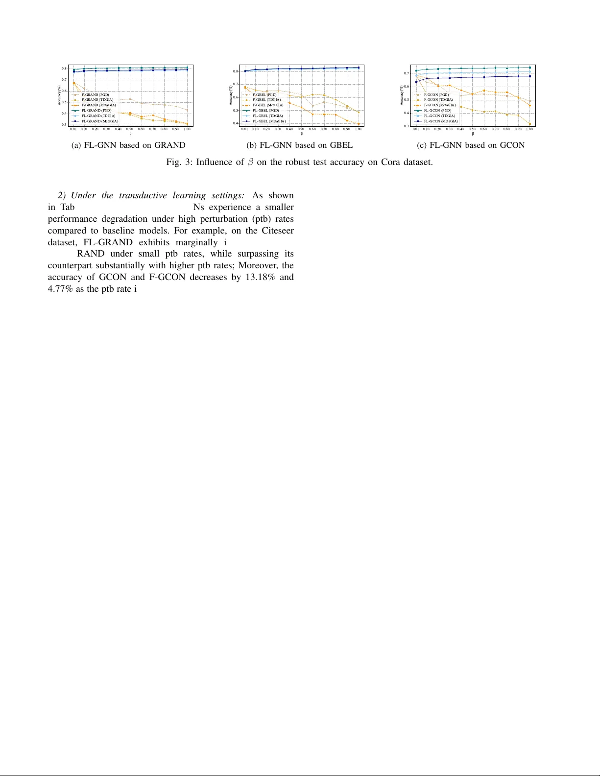
1 L yapuno v Stable Graph Neural Flo w Haoyu Chu, Xiaotong Chen, W ei Zhou, Senior Member , IEEE , W enjun Cui, Kai Zhao, Shikui W ei, Qiyu Kang Abstract —Graph Neural Networks (GNNs) ar e highly vulner - able to adversarial perturbations in both topology and features, making the learning of r obust r epresentations a critical challenge. In this work, we bridge GNNs with contr ol theory to introduce a novel defense framework grounded in integer - and fractional- order L yapuno v stability . Unlike con ventional strategies that rely on resour ce-hea vy adversarial training or data purification, our approach fundamentally constrains the underlying feature- update dynamics of the GNN. W e propose an adapti ve, lear nable L yapunov function paired with a nov el pr ojection mechanism that maps the network’ s state into a stable space, thereby offering theoretically prov able stability guarantees. Notably , this mech- anism is orthogonal to existing defenses, allowing for seamless integration with techniques like adversarial training to achieve cumulative rob ustness. Extensive experiments demonstrate that our L yapunov-stable graph neural flo ws substantially outperform base neural flows and state-of-the-art baselines across standard benchmarks and various adversarial attack scenarios. Index T erms —Graph neural flow , L yapunov stability , Adver- sarial attack, Certified r ob ustness. I . I N T RO D U C T I O N Graph neural networks (GNNs) hav e achie ved remarkable success and hav e found widespread application in numerous domains such as social network analysis [1], [2], traf fic flow prediction [3], [4], graph drawing [5], and molecular chem- istry [6]. Con ventional discrete GNNs, such as graph conv o- lutional networks (GCNs) [7] and graph attention networks (GA Ts) [8], propagate information between nodes through successiv e network layers. In recent years, driven by advances in continuous-time modeling techniques, GNN design guided by dynamical systems theory has emerged as a significant trend [9], [10]. The core idea underlying these kinds of GNN is to model the dynamic ev olution of the graph feature via ordinary or partial differential equations. Notable methods in this line of work include GRAND [11], which formu- lates information propagation via a heat diffusion equation; GRAND++ [12], extending GRAND with an additional source term; GREAD [13], which introduces a reaction term into the diffusion equation; and GraphCON [14], le veraging a second-order ordinary differential equation for dynamics mod- eling. These physically grounded formulations enhance the interpretability of the model and offer intuitive guidance for optimization and hyperparameter selection. Recognizing the demonstrated advantages of fractional differential operators in This work was supported in part by the Y oung Scientists Fund of the National Natural Science F oundation of China (No. 62506363) and the Fundamental Research Funds for the Central Univ ersities of Ministry of Education of China (No. 2025QN1151). (Corresponding author: Qiyu Kang.) Haoyu Chu is with the School of Computer Science and T echnology / School of Artificial Intelligence, China Univ ersity of Mining and T echnology , Xuzhou 221008, China (email: 6784@cumt.edu.cn). Qiyu Kang is with the School of Information Science and T echnology , Univ ersity of Science and T echnology of China, Hefei 230026, China. (email: kang0080@e.ntu.edu.sg) capturing comple x real-w orld phenomena [15], [16], Kang et al. [17] proposed FR OND, a frame work leveraging the non- local properties of fractional calculus to capture long-range dependencies during feature updates. Building on this, Cui et al. [18] introduced a flexible mechanism by parameterizing variable-order fractional deriv ati v es of hidden states through an auxiliary network. Despite these promising achiev ements, the security of GNNs faces severe threats from adversarial attacks. Adversar - ial examples, first introduced in computer vision [19], inv olve imperceptible perturbations to inputs that cause misclassifica- tions. Researchers hav e demonstrated that GNNs are similarly susceptible to adversarial attacks on the graph [20], [21]. While several graph adversarial defense strategies have been proposed to mitigate this issue, the underlying mechanisms remain unclear . In contrast, the dynamical systems perspectiv e has offered v aluable insights into the inherent stability prop- erties of graph-based learning, leading to the de velopment of new approaches aimed at enhancing GNN robustness. Y ang et al. [22] pioneered the robustness analysis of graph neural dif- fusion, theoretically and empirically demonstrating that such models exhibit intrinsic stability against graph perturbations. Subsequently , Kang et al. [23] demonstrated FR OND’ s ro- bustness from the perspective of fractional numerical stability . Zhao et al. [24] proposed Hamiltonian-inspired graph neural flows (HANG), leveraging energy conserv ation principles to enhance stability and mitigate the oversmoothing problem. In control theory , L yapunov stability theory establishes a foundational frame work for e v aluating system responses to initial perturbations, with established extensions to fractional- order dynamical systems. Furthermore, L yapunov theory has found applications in analyzing the stability of deep learning models [25], [26]. This naturally raises the question: Can L yapunov stability theory be le v eraged to pro vide rigorous the- oretical guarantees for the stability of dynamical system-based GNNs? Specifically , L yapunov methods comprise two primary approaches: the indirect method and the direct method [27]. The indirect method in volv es linearizing the nonlinear dynam- ical system near its equilibrium state and then judging stability based on the eigen values of the linearized system. The direct method characterizes stability by the L yapunov function (an abstract energy function), where a L yapunov stable dynamical system implies that its L yapunov function exists and it is positiv e definite and decreasing o ver time. T o this end, unlike con ventional defense methods such as adversarial training and detection, this work considers the robustness of GNNs from the dynamical systems perspective, providing a brand new certified robustness enhancement ap- proach based on the L yapunov stability theory . W e aim to constrain the graph neural flow to satisfy the conditions of L yapunov’ s direct method, which is simpler to implement than 2 the indirect method and can provide stricter stability criteria locally [28]. In addition, a special classification layer that can separate the equilibrium points is proposed to maximize the separation between the equilibrium points of different classes. As a result, when facing an input perturbation, the integer - and fractional-order L yapunov stable graph flow have the resilience to ev olv e to ward stable equilibrium points. Ex- perimental results demonstrate that the proposed models sig- nificantly outperform both the baseline integer and fractional graph neural flo w models. Furthermore, since our method is orthogonal to existing adversarial defenses, it can be combined with adv ersarial training to further enhance the rob ustness of GNN models. The remainder of this paper is structured as follows. Section II introduces related works on adversarial attacks and defenses on graphs, as well as the application of L yapunov theory in deep learning. Section III first establishes the necessary notations and preliminaries for graph neural networks, then provides the definition of L yapuno v stability and introduces L yapunov’ s direct method, co vering both the integer and fractional formulations. Section IV elaborates the proposed methodology , including the base fractional dynamical system, the integer- and fractional-order L yapunov stability module, and the equilibrium-separating classification layer . Section V provides comprehensi ve experiments and analyses to v erify the robustness of the proposed models across diverse adversarial scenarios. Finally , Section VI concludes the paper and outlines potential future research directions. The main contributions of this work are summarized as follows: • T o our knowledge, this work presents the first integration of L yapunov’ s direct method with graph neural flow , establishing a frame work for stability-guaranteed learning on graph datasets. • The proposed methodology is applicable to both integer - order and fractional-order dynamical systems, pro viding a comprehensiv e prov able robustness enhancement frame- work for a wide range of graph neural flo w models. • Extensive experiments demonstrate that the proposed ap- proach delivers consistent rob ustness performance gains across a wide spectrum of adversarial settings, including transductiv e and inductiv e black-box attacks as well as white-box attacks. • The proposed defense strategy is orthogonal to existing adversarial defense methods, enabling integration with strategies such as adversarial training to achie ve further improv ed robustness. I I . R E L A T E D W O R K S A. Adversarial Attacks and Defenses on Graph Adversarial attacks on graph are mainly categorized ac- cording to knowledge, objecti ves, and approaches. Regard- ing knowledge, black-box attacks lack access to the target model’ s internal details but can utilize graph data, while white- box attacks posses full model information [29]. Regarding objectiv es, poisoning attacks corrupt graph data to degrade model performance during training, whereas evasion attacks affect the inference of the trained model by altering input data [30]. Regarding approaches, modification attacks alter the original graph through edge changes or feature perturbations, while injection attacks introduce malicious nodes without manipulating the existing graph structure [31]. Adversarial defenses on graph include reactiv e methods and proactiv e methods. Reactiv e methods are characterized by their plug-and-play capability to resist adversarial attacks without retraining GNNs. For example, adversarial detection [32] uses a detector to identify anomalous edges or features in the input, adversarial purification [33] denoises adversarial perturbations in the input to restore clean graph structures or features typically by generativ e models. Proactive methods aim to enhance models’ rob ustness by modifying training data or internal mechanisms. For example, graph adversarial training methods [34] incorporate adversarial samples into the training dataset, network r obustification methods introduce stability constraints, such as Lipschitz constraints [35] or energy con- servation constraints [24], into graph neural networks. The proposed method falls under the category of network robustification. As an energy-based approach, we introduce energy dissipation other than conservation to driv e the state of graph neural flows tow ard a stable equilibrium point with minimal energy . B. Application of L yapunov theory in Deep Learning Recent adv ances hav e demonstrated the effectiv eness of combining L yapunov methods with neural network architec- tures to construct prov able certificates. Manek and K olter [36] introduced a scheme for the joint learning of a L yapunov func- tion and stable dynamics, with the application of this technique in physical simulation and video te xture generation. Storm et al. [25] de veloped a rob ustness assessment framework for multilayer perceptron using finite-time L yapunov exponents (FTLE), which can characterize the gro wth or decay of local perturbations in forward propagation. Chu et al. [37] proposed a L yapunov stable deep equilibrium model for defending adversarial attacks on images. Follo wing the emergence of neural ordinary differential equations (Neural ODEs) [38], there has been growing interest in integrating L yapunov theory with these continuous-depth models. Kang et al. [39] employed L yapunov’ s indirect method to enhance the robustness of Neural ODEs. Schlaginhaufen et al. [40] introduced a novel regularization term based on L yapunov-Razumikhin functions to stabilize neural delay dif- ferential equations. Building on LaSalle’ s in v ariance principle (a generalization of L yapunov’ s method), T akeishi et al. [41] dev eloped Neural ODEs that are capable of handling stability for general inv ariant sets, including limit cycles and line attractors. I I I . N OTA T I O N A N D P R E L I M I N A R I ES W e define an undirected graph without self-loops as G := ( V , W ) , where V = 1 , . . . , N denotes a collection of N nodes, |V | = N , The weighted connections between nodes are encoded in an adjacency matrix W := ( W ij ) ∈ R N × N , where each entry W ij corresponds to the weight of the edge linking node i to node j , satisfying W ij = W j i (that is, W is 3 symmetric). Let U =  [ u (1) ] ⊤ , · · · , [ u ( N ) ] ⊤  ⊤ ∈ R |V |× d be the features of the node, which is a matrix composed of row vectors ( u ( i ) ) ⊤ ∈ R d , with i being the index of the node. A typical integer -order dynamical system can be described by a first-order ODE: d u d t = f ( t, u ( t )) , (1) where u ( t ) represents the state of the system at time t , and f defines the dynamics that governs the ev olution of the system. If the function f does not explicitly depend on time t , the dynamical system is autonomous. In the analysis of such dynamical systems, the L yapunov stability theory provides a fundamental framework for studying the behavior of solutions without explicitly solving the dif ferential equations. Definition 1 (L yapunov stability) . An equilibrium u ⋆ is called stable in the L yapunov sense if, for an y gi v en ε > 0 , there exists δ > 0 such that whenever the initial condition satisfies ∥ u (0) − u ⋆ ∥ < δ , the solution remains within ∥ u ( t ) − u ⋆ ∥ < ε for all t ≥ 0 . Suppose u ⋆ is stable and satisfy lim t →∞ ∥ u ( t ) − u ⋆ ∥ = 0 , it is termed asymptotically stable. Further , suppose u ⋆ is stable and there exists some ν > 0 such that lim t →∞ ∥ u ( t ) − u ⋆ ∥ e ν t = 0 , it is termed asymptotically stable. Theorem 2 (L yapunov’ s direct method [42]) . Giv en a fixed point u ⋆ , suppose there exists a continuously differentiable function V : [0 , ∞ ) × U → R defined for t ≥ 0 in a neighborhood U of u ⋆ , fulfilling the following conditions: (1) V attains its minimum at u ⋆ for all t ≥ 0 . (2) Along every solution trajectory in U other than the equilibrium u ⋆ , V decreases strictly . then V is called a L yapunov function, and the equilibrium u ⋆ is asymptotically stable. Furthermore, u ⋆ is e xponentially stable if, in addition, there exist positive constants c and K ( α ) such that: (3) ∥ u ∥ 2 ≤ V ( t, u ) ≤ K ( α ) ∥ u ∥ 2 , ∀ u ∈ { u : ∥ u ∥ ≤ α } ; (4) ˙ V ( t, u ) ≤ − cV ( t, u ) , c > 0 . T o accommodate a broader range of application scenarios, we also consider fractional-order systems. Let u be a state vector in a state space, the dynamics of the non-autonomous fractional-order system is described by D β t u ( t ) = f ( t, u ) . (2) Here, we adopt the follo wing definition of the Caputo frac- tional deriv ati ve [43]: D β t u ( t ) := 1 Γ(1 − β ) Z t 0 ( t − τ ) − β u ′ ( τ ) dτ , (3) where β ∈ (0 , 1] denotes fractional order , Γ is the Gamma function, , and u ′ ( · ) denotes the first deri v ativ e of a differ - entiable function u ( t ) . When β = 1 , D 1 t u ( t ) = d u /dt , and Eq. (2) reduces to the first-order ODE (1). T o demonstrate the fractional-order extension of L yapunov’ s direct method, we first introduce the concept of Mittag–Leffler stability . Definition 3 (Mittag–Leffler stability) . A fractional dynamical system is called Mittag–Leffler stable if ∥ u ( t ) ∥ ≤ m [ u (0)] E β ( − λ ( t ) β ) b , (4) where λ ≥ 0 , b > 0 , the function m ( · ) fulfills m (0) = 0 , m ( u ) ≥ 0 , and is locally Lipschitz on u ∈ R n . Here E β ( z ) = ∞ X k =0 z k Γ( k β + 1) (5) is the Mittag–Leffler function [43]. In the case where β = 1 , this function reduces to the familiar e xponential function. Remark 1. W ithin the fr amework of fractional-or der dynam- ics, Mittag–Leffler stability serves as a key criterion. If a system is Mittag-Lef fler stable , it is inher ently asymptotically stable. Theorem 4 (Fractional L yapunov’ s direct method [44]) . Let u ⋆ be an equilibrium of a fractional-order system and D ⊂ R n a region containing the origin. Assume there exists a function V ( t, u ( t )) : [0 , ∞ ) × D → R that is continuously differentiable and locally Lipschitz in u , and suppose for some positiv e con- stants α i ( i = 1 , 2 , 3) , a, b , this candidate L yapuno v function satisfies α 1 ∥ u ∥ a ≤ V ( t, u ( t )) ≤ α 2 ∥ u ∥ ab , (6) and D β t V ( t, u ( t )) ≤ − α 3 ∥ u ∥ ab . (7) Then the system is Mittag–Lef fler stable. Remark 2. The inte ger-or der L yapunov stability theor em emer ges as a particular instance of the above r esult when the fractional or der is set to β = 1 . I V . M E T H O D O L O G Y This section presents the proposed framew ork for enhancing the robustness of GNNs through the lens of L yapunov stability theory . W e begin by introducing the base graph neural flo w , which formulates the node feature e volution as either an integer -order or fractional-order dynamical system. Next, we detail the integer- and fractional-order L yapunov stability mod- ule, a nov el mechanism that projects the base dynamics into a L yapunov-stable space via a learnable L yapunov function. W e then describe the architecture and training pipeline of the resulting L yapuno v stable GNNs, which integrate the stability module with an equilibrium-separating classification layer to maximize inter-class mar gin while preserving stability . Finally , we provide a theoretical analysis of certified robustness under perturbation, demonstrating that the proposed models exhibit robustness, and thus prov able resilience against adversarial perturbations. A. The Base Gr aph Neural Flow The node feature update process can be modeled as a time- ev olving feature extraction procedure, where the differential equation describes the information propagation between nodes. Let U ( t ) denote the node features at time t , and let F ( · ) 4 𝐔(0) 𝐔(𝑡 ! ) 𝐔(𝑡 " ) Time e volut ion Long-range memorie s (F ractional ca s e) 𝐔 ∗ Base graph neural flow Integral-order: d𝐔 𝑡 /d𝑡 % = ℱ 𝑡 , 𝐔 𝑡 ; 𝐖 Fractional-order: %𝐷 ! " 𝐔 𝑡 = ℱ (𝑡, 𝐔 𝑡 ; 𝐖) L yapunov-sta ble graph neural flow Integral-order: d𝐔 𝑡 /d𝑡 % = ℱ . (𝑡 , 𝐔 𝑡 ; 𝐖) Fractional-order : 𝐷 ! " 𝐔 𝑡 = ℱ . (𝑡 , 𝐔 𝑡 ; 𝐖) Projection !𝜎 !𝜎 !𝜎 !𝜎 !𝜎 !𝜎 !𝜎 !𝜎 !𝜎 ICNN & &𝑡 𝑼 & 𝑉 L yapunov func tion 𝑉 Feature attac k T opology attack Baseline model i s more prone to misclassificati on . Gound truth label Pr ediction: Energy Dissipation The proposed model can c lassify corr ectly . Pr ediction: Fig. 1: The scratch of the L yapunov stability module. The black dashed box illustrates the dynamic ev olution of the base graph neural flow over the time interv al [0 , t n ] , where the fractional case captures long-range memories by incorporating historical states, unlike the integer -order’ s behavior depends solely on the current state. The orange dashed box depicts the projected L yapunov-stable system, which satisfies the conditions of the L yapunov’ s direct method, where the L yapunov function is implemented by an input-conv ex neural network, a fully connected neural netw ork with special properties. represent the governing equation, the dynamic evolution of graph nodes can be expressed as a system of ODEs: d U ( t ) d t = F ( t, U ( t ); W ) (8) with the initial condition U (0) , where U ( t ) =  h u (1) ( t ) i ⊤ , · · · , h u ( N ) ( t ) i ⊤  ⊤ . Integer -order differential equations gov ern systems whose behavior depends solely on the current state, whereas fractional-order differential equations (FDEs) correlate a series of past states with the current state. This property grants them a distinct advantage in modeling non-uniform dynam- ical behaviors in complex networks, enabling more accurate characterization of cumulativ e memory effects and non-local properties. By incorporating the Caputo fractional deriv ati ve, this dynamic process can be reformulated as a fractional-order ODE: D β t U ( t ) = F ( t, U ( t ); W ) (9) with initial condition U (0) . The final node features U ( T ) , which can be used for node classification, can be obtained by solving this equation up to a terminal time t = T . B. Inte ger- and F ractional-Or der Lyapunov Stability Module Due to inherent cognitive deficiencies of deep neural net- works, the robustness of both integer -order and fractional- order differential equation-based GNNs remains challenging to guarantee. W e consider the failure of the current GNNs on adversarial examples to be the neglect of preserving the underlying stability structure. Therefore, we propose to impose a hard constraint concerning L yapunov stability on the graph neural flow and introduce a family of L yapunov-stable GNNs, which encompass the integer-order L yapunov-stable GNNs (IL-GNNs) and the fractional-order L yapunov-stable GNNs (FL-GNNs). The core innov ation lies in the unified L yapunov stability module, which integrates graph neural flo w with L yapunov theory to ensure the robustness of the GNN dynamics. This module applies L yapunov’ s direct method to ensure that the node features ev olve in a stable manner , avoiding unbounded growth or oscillations, thereby enhancing resilience against adversarial attacks. Specifically , the stability module is de- signed by constructing a L yapuno v function V that satisfies the conditions of Theorem 2 for the case of inte ger-order ( int ) or Theorem 4 for the case of fractional-order ( frac ) and projecting the base GNN dynamics onto a stable manifold. Figure 1 shows the scratch of the fractional L yapunov stability module. Let U ⋆ be the equilibrium points of the GNN dynamics, the L yapunov-stable module is defined as ˆ F ( t, U ⋆ ; W ) =        F ( t, U ⋆ ) if ϕ ( t, U ⋆ ) ≤ 0 , F ( t, U ⋆ ) − ∇ V ϕ ( t, U ⋆ ) ∥∇ V ( U ⋆ ) ∥ 2 otherwise (for int ) , F ( t, U ⋆ ) − D β t V ϕ ( t, U ⋆ ) ∥ D β t V ∥ 2 otherwise (for frac ) , (10) where ϕ ( t, U ⋆ ) = ∇ V ⊤ F + cV for the case of integer -order 5 and ϕ ( t, U ⋆ ) = D β t V + α 3 ∥ U ⋆ ∥ for the case of fractional- order . Assuming ϕ ( t, U ⋆ ) > 0 holds, the output of the basic model will be refined by projection operation, otherwise the output is returned unchanged. It is worth mentioning that the gradient is multiplied by the numerator, which prev ents the gradient from v anishing theoretically . The function V is constructed as a trainable neural network that is designed to meet the conditions of a L yapunov function: V = σ ( ICNN ( U ⋆ ) − ICNN ( 0 )) + ∥ U ⋆ ∥ 2 , (11) where σ represents a positive con vex acti v ation function sat- isfying σ (0) = 0 , and ICNN refers to an input-con vex neural network [45]: q 1 = σ 0  W I 0 U ⋆ + b 0  , q i +1 = σ i  P i q i + W I i U ⋆ + b i  , i = 1 , . . . , k − 1 , g ( U ⋆ ) ≡ q k , (12) where W I i , b i denote the weights and biases of the i -th layer, respectiv ely . P i are positive weights. σ is con ve x and non- decreasing acti v ation function to guarantee that each layer’ s operation maintains con ve xity , which can be chosen as smooth version of ReLU function [36]: σ ( x ) =      0 , if x ≤ 0 , x 2 / (2 d ) , 0 < x < d, x − d/ 2 , x ≥ d. (13) By incorporating this projection mechanism, the resulting graph nerual flo w is guaranteed to meet the requirements of the integer- or fractional-order L yapuno v’ s direct method. Consequently , the equilibrium points of the projected model are ensured to be L yapunov stable for the integer-order case or Mittag–Leffler stable for the fractional-order case. C. L yapunov Stable GNNs and their T raining Pr ocess The proposed L yapunov stable GNNs contain three key components, namely the base graph neural flow , the L yapunov stability module, and an equilibrium-separating classification layer . The dynamical system parameterized by IL-GNNs and FL-GNNs can be formalized as follows: d U ( t ) d t = Pro j( F , {F : ∇ V T F ≤ − cV ( t, U ) } ) , (14) D β t U ( t ) = Pro j( F , {F : D β t V ≤ − α 3 ∥ U ∥} ) , (15) where Pro j denotes the projection sho wn in Eqn.(10), and F can be chosen as one of the base dynamical systems. 1) Choices of the base dynamical system: W e consider three kinds of integer-order base dynamical system, namely GRAND [11], GraphBel [22] and GraphCON (GCON) [14], and their corresponding fractional-order extensions as the gov erning equations. GRAND and Fractional-GRAND models (F-GRAND) are gov erned by d U ( t ) d t = ( A ( U ( t )) − I ) U ( t ) , (16) D β t U ( t ) = ( A ( U ( t )) − I ) U ( t ) , (17) respectiv ely , where I ∈ R N × N is an identity matrix, A ( U ( t )) is a time-dependent learnable attention matrix: A = a ( u i , u j ) = softmax  ( W K u i ) ⊤ W Q u j d k  , (18) where W K and W Q are learnable matrices, and d k is a hyperparameter . GraphBel and Fractional-GraphBel models (F-GBel) are defined as d U ( t ) d t = ( A s ( U ( t )) ⊙ B s ( U ( t )) − Ψ ( U ( t ))) U ( t ) , (19) D β t U ( t ) = ( A s ( U ( t )) ⊙ B s ( U ( t )) − Ψ ( U ( t ))) U ( t ) , (20) respectiv ely , where ⊙ denotes the element-wise multiplication, A s ( · ) is a learnable attention function, B s ( · ) represents a normalization function, Ψ ( u , u ) = P v ( A s ⊙ B s )( u , v ) . GCON and Fractional-GraphCON model (F-GCON) can be formalized as      d U ( t ) d t = σ ( F ( U ( t ) , t ; W )) − γ U ( t ) − α Y ( t ) , d Y ( t ) d t = U ( t ) . (21) ( D β t U ( t ) = σ ( F ( U ( t ) , t ; W )) − γ U ( t ) − α Y ( t ) , D β t Y ( t ) = U ( t ) . (22) respectiv ely , where ζ is an activ ation function, γ and α are hyperparameters. The inte ger deriv ativ es are obtained by automatic dif feren- tiation, and the fractional deri v ati ves are computed using the fractional Adams–Bashforth scheme [46]. 2) Details of stability module: The ICNN architecture is specifically designed to ensure con vexity of the output with respect to the input variables, making it particularly suitable for learning L yapunov functions. It is implemented in this work as a two-layer feedforward neural network, which is composed of linear transformations, smooth version of ReLU activ ation functions, and skip connections as formalized in Eqn.(12). The L yapunov stability module is built upon the ICNN to enforce the necessary conditions for a valid L yapunov function, combining the ICNN output with a stabilization term to ensure positi ve definiteness. The module constructs a L yapuno v candidate and then maps the base system into a L yapunov stable half-space. 3) The equilibrium-separating classification layer: While stable equilibrium points can provide local robustness, their direct application to graph node classification faces a critical challenge. That is, equilibrium points corresponding to differ - ent classes may lie in close proximity , resulting in small and ov erlapping stability neighborhoods. This phenomenon may potentially diminish adversarial rob ustness, where perturba- tions can possibly push input across the decision boundary . T o mitigate this problem, we augment the fractional L yapunov stability module with an equilibrium-separating layer , which explicitly maximizes the separation between equilibriums of different classes while preserving stability guarantees. Let U ′ denote the output of the L yapunov stability module. T o enforce separation between class-wise equilibrium points, we employ 6 a fully connected layer to output the parametrized form of U ′ , ensuring orthogonality via the constraint ( U ′ ) ⊤ U ′ = I . 4) The training pr ocess: The training process for L yapunov stable GNNs contains two stages. In the first stage, we train the base dynamical system until con ver gence. T o determine whether the base dynamical system has reached an equilibrium state during the training, we monitor the training accurac y o ver successiv e epochs and declare con vergence to an equilibrium when the fluctuations in accuracy fall belo w a predefined small threshold. In the second stage, we focus on training the L yapunov stability module, mainly updating the parameters of the ICNN and the equilibrium-separating classification layer . D. Certified Robustness under P erturbation W e in vestigate the impact of initial adversarial perturbations on the model’ s behavior . Our analysis begins by establishing the robustness of the integer -order case, subsequently ex- tending these findings to the fractional-order frame work. It should be noted that in FR OND [23], the fractional extension of numerical stability analysis is applied to compare the numerical results of the model before and after adversarial perturbations, focusing on whether the accumulation of er- rors remains controlled when numerically solving FDEs. The difference between the two results is bounded by an upper bound, leading to the conclusion that FR OND exhibits inherent robustness against perturbations. For L yapunov stable GNNs, the research problem revolv es around whether the solutions of the continuous inte ger- and fractional-order dynamical systems deviate from the original solutions or conv er ge to equilibrium points under minor adversarial perturbations. Here, we show that when the node features at the initial time are subjected to initial perturbations, the systems can exhibit robustness against perturbations. Proposition 5. The equilibrium points of the projected integer -order dynamical system defined in Eqn.(14) are ex- ponentially stable. Pr oof. From Eqn.(13), it can be seen that when x takes values in [0 , ∞ ) , the activ ation function σ is linear , whereas when x takes v alues in (0 , d ) , σ is quadratic. Therefore, the function V has both upper and lower bounds. That is, ∀ α > 0 , assuming U ∈ { U : ∥ U ∥ ≤ α } , there exists a positiv e constant K ( α ) such that ∥ U ∥ 2 ≤ V ( t, U ( t )) ≤ K ( α ) ∥ U ∥ 2 , that is, the first condition of Theorem 2. Since the projected system defined in Eqn.(14) satisfies condition (4) of Theorem 2, we ha ve, dV ( t, U ( t )) V ( t, U ( t )) ≤ − cdt. Integrating both sides of the abov e equation yields V ( t, U ( t )) ≤ V (0 , U (0)) e − ct ( t ≥ 0) . Therefore, we can further obtain ∥ U ∥ 2 ≤ V (0 , U (0)) ≤ K ( α ) ∥ U (0) ∥ 2 e − ct . This implies ∥ U ∥ ≤ K ( α ) | U (0) ∥ e − ct/ 2 . Hence, the equi- librium points U ⋆ are exponentially stable. Proposition 6. The equilibrium points of the projected fractional-order dynamical system defined in Eqn.(15) are Mittag-Leffler stable. Pr oof. Let a = 2 and b = 1 , the function V satisfies the first condition of Theorem 4: α 1 ∥ U ∥ 2 ≤ V ( t, U ( t )) ≤ α 2 ∥ U ∥ 2 , (23) Since the projection operation ensure the fractional system satisfied Eqn.(7), there e xists a nonne gati ve function M ( t ) satisfying D β t V ( t, U ( t )) + M ( t ) = − α 3 α 2 V ( t, U ( t )) . (24) Performing the Laplace transform of Eqn.(24) gi ves, s β V ( s ) − V (0) s β − 1 + M ( s ) = − α 3 α 2 V ( s ) , where s represents the v ariable in Laplace domain. By lev eraging Lipschitz condition and the in verse Laplace transform, we can obtain the solution of Eqn.(24): V ( t ) = V (0) E β ( − α 3 α 2 t β ) − M ( t ) ∗  t β − 1 E β ( − α 3 α 2 t β )  | {z } ≥ 0 ≤ V (0) E β ( − α 3 α 2 t β ) . (25) Substituting Eqn.(25) to Eqn.(23), we have ∥ U ( t ) ∥ ≤  mE β ( − α 3 α 2 t β )  1 2 , (26) where m = V (0 , U (0)) /α 1 ≥ 0 and m = 0 holds if and only if U (0) = 0 , which imply the projected equilibrium points are Mittag–Leffler stable. Remark 3. The pr oposed L yapunov stable GNNs can be viewed as special association memory networks [47], wher e the functionality of association memory is modeled by an ener gy function and the equilibrium points (the local minima of the ener gy) serve as memories. The ener gy landscape of the system is shaped by the L yapunov function, which ensur es the positive definiteness and monotonic decr ease over time, corr esponding to the process of writing information into the network (i.e. learning). The dynamical trajectory of the system r epresents the memory recall (i.e. infer ence), wher e featur es evolve towar d stable equilibrium points. F r om this point of view , an association occurs between the initial state of the system and its asymptotic state. The stability pr operty ensur es that small perturbations to the initial state (pr ovided the y r emain within the basin of attraction) are automatically corr ected by the system dynamics, aligning with the certified r obustness of the proposed models. 7 T ABLE I: Benchmarks details and the attacks’ s b udgets of graph injection attacks (GIA) Dataset # Nodes # Edges # Features # Classes max # Nodes (for GIA) max # Edges (for GIA) Cora 2708 5429 1433 7 60 20 Citeseer 3327 4732 3703 6 90 10 Computers 18333 81894 6805 15 300 150 PubMed 19717 44338 500 3 200 100 T ABLE II: Node classification accuracy (%) on graph injection, ev asion, non-tar geted, black-box attack in INDUCTIVE learning. Results under adversarial attacks that surpass the competing methods are bold . Second best results are with the underline Dataset Attack GRAND IL-GRAND F-GRAND FL-GRAND GBel IL-GBel F-GBel FL-GBel GCON IL-GCON F-GCON FL-GCON HANG Cora clean 82.24±1.82 88.88±0.97 86.44±0.31 88.95±0.39 79.07±0.46 85.73±0.73 77.55±0.79 86.74±0.93 83.10±0.63 86.97±0.60 82.42±0.89 87.10±0.80 87.13±0.86 PGD 36.80±1.86 79.01±1.24 56.38±6.39 80.76±0.33 63.93±3.88 80.86±0.73 69.50±2.83 82.60±0.67 48.38±2.44 72.71±0.38 56.70±4.36 74.28±0.69 78.37±1.84 TDGIA 40.0±3.52 73.41±1.17 54.88±6.72 78.06±0.39 53.22±2.95 73.67±1.21 56.94±1.82 81.87±0.60 46.43±2.82 60.46 ±3.85 54.24±2.54 77.06±0.73 79.76±0.99 MetaGIA 37.89±1.56 74.64±1.64 53.36±5.31 78.69±0.36 66.74±3.23 82.20±1.66 71.98±1.32 82.84±0.56 52.21±2.71 61.56±1.51 63.97±2.09 67.74±0.92 77.48±1.02 Citeseer clean 72.52±0.73 75.47±0.64 71.91±0.43 75.66±0.48 74.75±0.28 74.58±0.70 71.09±0.30 75.03±0.47 72.07±0.93 63.08±1.02 73.50±0.43 74.61±0.80 74.11±0.62 PGD 42.20±2.77 71.62±1.39 61.26±1.23 72.04±1.23 47.73±5.87 72.79±0.52 60.78±2.37 73.22±1.23 37.71±7.0 61.03±0.95 54.47±1.0 61.52±0.77 72.31±1.16 TDGIA 30.02±1.33 71.65±0.64 50.74±1.20 73.14±0.47 47.88±1.83 71.68±1.33 65.52±0.55 72.17±0.79 30.93±3.00 60.19±0.83 54.71±1.69 64.08±0.98 72.12±0.52 MetaGIA 30.42±1.87 71.98±1.32 55.50±1.72 72.17±0.97 39.13±1.19 72.28±0.74 60.85±1.88 73.31±0.59 29.09±2.01 66.93±0.84 48.82±3.27 70.52±0.94 72.92±0.66 Computers clean 92.53±0.34 90.43±0.26 92.61±0.20 90.44±0.13 88.12±0.33 87.48±0.55 88.02±0.24 87.98±0.51 91.30±0.20 91.44±0.25 91.86±0.38 91.63±0.31 - PGD 70.45±11.03 89.89±0.30 89.90±1.33 90.02±0.33 87.38±0.37 87.32±0.57 87.60±0.33 87.66±0.60 81.28±7.99 91.11±0.28 91.36±0.74 91.55±0.27 - TDGIA 65.45±14.30 91.13±0.21 84.71±1.52 90.44±0.19 87.67±0.40 87.69±0.49 87.81±0.28 87.91±0.48 68.70±15.67 90.75±0.25 90.45±0.71 90.63±0.31 - MetaGIA 70.01±9.32 89.71±0.43 87.50±3.17 90.23±0.36 87.77±0.22 87.94±0.56 87.37±0.23 87.97±0.55 82.43±8.42 91.75±0.25 90.51±0.88 91.26±0.57 - Pubmed clean 88.44±0.34 86.89±0.65 88.39±0.47 87.43±0.42 88.18±1.89 90.25 ±0.20 89.51±0.12 93.78±0.13 88.09±0.32 86.73±0.25 90.30±0.11 87.27±0.74 89.93±0.27 PGD 44.61±2.78 63.01±0.40 59.62±11.66 61.74±0.31 67.81±12.23 69.06±0.26 72.04±2.08 74.18±0.09 45.85±1.97 61.49±0.29 51.16±6.04 61.77±0.22 81.81±1.94 TDGIA 46.26±1.32 60.10±0.94 54.31±2.38 60.64±1.10 68.66±10.64 73.15±0.34 72.49±0.83 72.93±0.18 45.57±2.02 69.81±0.33 55.50±4.03 70.21±0.32 86.62±1.05 MetaGIA 44.07±2.11 66.93±0.40 61.62±9.05 68.68±1.24 64.64±9.70 76.13±0.32 79.16±0.87 80.20±0.19 45.81±2.81 56.63±0.25 52.03±5.53 56.11±0.69 87.58±0.75 T ABLE III: Classification accuracy (%) under modification, poisoning, non-targeted attack (Metattack) in TRANSDUCTIVE learning Dataset Ptb(%) GRAND IL-GRAND F-GRAND FL-GRAND GBel IL-GBel F-GBel FL-GBel GCON IL-GCON F-GCON FL-GCON HANG Cora 0 82.24±1.82 78.56±0.39 81.25±0.89 81.75±0.75 80.28±0.87 79.32±0.49 79.05±0.73 78.40 ±0.18 83.10±0.79 80.67±0.09 80.91±0.54 80.00±0.06 - 5 78.97±0.49 77.04±0.49 78.84±0.57 81.04±0.12 77.70±0.66 77.53±0.47 76.10±0.74 76.26±0.55 77.90±1.14 77.11±0.21 77.80±0.44 76.20±0.33 - 10 75.02±1.25 76.58±0.15 76.61±0.15 80.08±0.29 74.30±0.88 74.19±0.21 74.03±0.47 75.15±0.29 72.53±1.08 75.55±0.20 74.63±1.42 75.20±0.52 - 15 71.43±1.09 76.48±0.17 73.42±0.97 79.83±0.27 72.14±0.69 72.35±0.70 73.01±0.75 74.31±0.63 69.83±0.68 73.99±0.27 73.01±0.78 73.22±0.55 - 20 60.53±1.99 76.48±0.20 69.27±2.10 78.20±0.43 65.41±0.99 72.91±0.48 69.35±1.23 73.64±0.09 57.28±1.62 72.48±0.22 69.23±1.35 72.99±0.39 - 25 55.26±2.14 75.99±0.20 64.47±1.83 76.70±0.60 62.31±1.13 71.72±0.33 67.63±0.93 72.72±0.22 53.17±1.52 70.02±0.73 65.27±1.33 72.17±0.61 Citeseer 0 71.50±1.10 71.94±0.31 71.37±1.34 71.65±0.49 71.37±1.34 71.05±0.43 68.90±1.15 71.06±0.22 70.48±1.18 71.42±0.38 71.49±0.71 70.46±0.14 - 5 71.04±1.15 71.61±0.43 71.47±0.96 69.89±0.16 68.45±1.02 70.24±0.65 68.36±0.93 70.66±0.14 69.75±1.63 70.33±0.62 70.77±1.15 70.89±0.45 - 10 68.88±0.60 71.27±0.83 69.76±0.71 69.78±0.12 69.54±0.82 69.12±0.10 66.72±1.31 70.20±0.38 67.40±1.78 70.51±0.19 69.54±0.82 70.93±0.24 - 15 66.35±1.37 69.40±0.57 67.94±1.42 68.43±0.22 63.63±1.67 68.73 ±0.23 63.56±1.95 69.98±0.15 65.78±1.97 70.00±0.83 67.37±0.87 70.30±0.26 - 20 58.71±1.42 68.62±0.32 64.18±0.93 68.03±0.13 58.90±0.84 66.56 ±0.32 63.38±0.96 68.37±0.15 56.79±1.46 70.03±0.07 66.52±0.68 70.23±0.21 - 25 60.15±1.37 65.30±0.20 65.46±1.12 67.23±0.12 61.24±1.28 65.18±0.22 64.60±0.48 67.71±0.17 57.30±1.38 69.77±0.10 66.72±1.12 69.20±0.23 - Pubmed 0 85.06±0.26 81.61±0.04 82.28±0.10 85.67±0.08 84.02±0.26 82.17±0.03 86.15±0.14 86.18±0.01 84.65±0.13 83.52±0.03 87.19±0.09 87.23±0.03 85.08±0.20 5 84.11±0.30 79.24±0.04 81.27±0.21 85.56±0.03 83.91±0.26 82.13±0.12 85.91±0.14 85.93±0.02 83.06±0.22 79.58±0.03 86.38±0.19 86.58±0.12 85.08±0.18 10 84.24±0.18 76.11±0.11 80.64±0.19 85.31±0.06 84.62±0.26 81.55±0.09 85.90±0.20 85.48±0.01 82.25±0.12 76.35±0.02 85.90±0.20 86.13±0.15 85.17±0.23 15 83.74±0.34 72.64±0.07 79.95±0.25 85.09±0.02 84.83±0.20 81.06±0.06 85.45±0.33 85.34±0.28 81.26±0.33 72.92±0.12 85.78±0.37 85.90±0.01 85.0±0.22 20 83.58±0.20 70.38±0.08 79.96±0.21 84.54±0.09 84.89±0.45 81.29±0.04 85.44±0.16 85.03±0.41 81.58±0.41 70.31 ±0.02 85.55±0.02 85.74±0.19 85.20±0.19 25 83.66±0.25 68.15±0.03 79.95±0.26 84.22±0.03 85.07±0.15 80.95±0.10 85.19±0.14 85.15±0.11 80.75±0.32 68.06±0.05 85.37±0.23 85.83±0.17 85.06±0.17 T ABLE IV: Node classification accuracy (%) on graph injection, ev asion, non-targeted, white-box attack in inductive learning. A T is the abbreviation for adversarial training. Dataset Attack GRAND IL-GRAND FL-GRAND FL-GRAND+A T GBel IL-GBel FL-GBel FL-GBel+A T GCON IL-GCON FL-GCON FL-GCON+A T HANG Cora clean 87.53±0.59 89.12±0.23 89.58±0.60 89.24±0.84 86.13±0.51 86.47±0.58 87.03±1.06 85.79±0.84 84.69±1.10 87.97±0.23 85.53±0.96 87.13±0.86 88.31±0.48 PGD 36.02±4.09 70.01±0.88 72.22±0.64 72.75±0.91 37.16±1.69 59.87±2.26 59.43±2.43 61.35±1.96 35.83±0.71 53.45±1.01 52.96±1.19 53.90±1.24 67.69±3.84 TDGIA 14.72±1.97 58.55±1.34 56.65±2.91 59.32±1.84 15.46±1.98 66.98±2.14 67.54±2.01 69.12±2.46 33.05±1.09 55.14±1.96 54.44±1.40 55.90±2.95 64.54±3.95 Citeseer clean 74.98±0.45 74.66±0.63 75.03±0.66 74.88±0.59 69.62±0.56 74.56±1.17 74.69±1.19 73.04±0.51 74.84±0.49 64.09±2.48 74.36±1.04 73.51±2.00 74.11±0.62 PGD 38.57±1.94 66.58±0.77 66.79±0.98 67.97±1.16 32.24±1.21 67.02±1.25 66.21±1.50 70.46±2.13 42.78±1.54 52.00±4.27 58.23±4.69 65.23±1.19 67.54±1.52 TDGIA 30.11±1.43 54.91±0.66 54.31±0.86 55.37±0.45 16.26±1.20 75.35±0.58 75.63±0.77 76.09±0.79 33.55±1.10 66.14±1.38 66.46±0.99 67.01±2.04 63.29±3.15 V . E X P E R I M E N T S This section elaborates on the experimental setup and comprehensiv e performance analysis. W e select representativ e benchmarks tailored to the task characteristics, with stan- dardized pre-processing to ensure reproducibility and fairness. For comparison, we adapt several state-of-the-art models to comprehensiv ely ev aluate the performance advantages of the proposed approach. In our experiments, all implementations are dev eloped in PyT orch [48] and executed on a single NVIDIA GeForce R TX 3090 GPU with 24GB of memory . The source codes are a v ailable at https://anonymous.4open. science/r/test- LSGNF. A. The Experimental Setup 1) Datasets: W e e valuate the f amily of L yapunov sta- ble GNNs, namely the IL-GNNs and FL-GNNs, on four datasets, including different graph-structures, such as citation networks and co-purchasing graphs. Citation networks, such as Cora [49], Citeseer [50], and Pubmed [51], represent academic articles as nodes and citation relationships as edges. The features of each node typically include text embeddings or topic distributions of the article, while the node labels correspond to the classification of the article. Co-purchasing graphs, such as Computer [52], model products as nodes, with edges indicating frequently co-purchased item pairs. These 8 T ABLE V: Classification accurac y (%) of the IL- and FL-GNNs without equilibrium-separating (ES) layer on graph injection, ev asion, non-tar geted attack in inductive learning Dataset Attack IL-GRAND (w/o ES layer) IL-GBel (w/o ES layer) IL-GCON (w/o ES layer) FL-GRAND (w/o ES layer) FL-GBel (w/o ES layer) FL-GCON (w/o ES layer) Cora clean 87.77±1.01 86.29±1.07 85.47±0.75 88.18±1.38 85.98±1.53 84.33±0.46 PGD 78.88±0.92 79.75±0.46 70.27±0.72 78.84±1.24 78.00±0.87 70.18±0.89 TDGIA 72.40±0.83 74.06±1.27 69.62±0.96 74.76±1.18 74.78±0.99 76.43±1.31 MetaGIA 76.44±0.89 76.20±0.87 61.50±1.51 76.98±0.58 83.02±1.54 64.08±1.55 Citeseer clean 73.39±0.85 72.93±0.63 66.70±1.68 73.26±1.08 73.52±1.13 63.47±1.18 PGD 70.79±0.80 71.98±1.41 60.84±0.94 71.21±0.65 72.29±1.37 61.12±0.36 TDGIA 71.76±0.59 71.28±0.76 63.95±1.68 72.26±0.72 71.73±1.20 62.21±1.98 MetaGIA 71.03±0.79 71.66±0.93 63.89±1.13 70.90±0.48 72.45±0.50 65.11±1.64 Pubmed clean 87.87±0.53 87.14±0.29 85.12±0.42 86.49±0.28 87.10±0.32 84.48±0.49 PGD 64.79±0.26 73.27±0.27 61.88±0.91 61.99±0.91 73.19±0.30 60.25±0.72 TDGIA 60.21±0.54 73.43±0.18 71.56±0.35 59.40±0.27 72.80±0.19 69.58±0.46 MetaGIA 60.42±0.77 74.12±0.33 50.83±0.28 65.78±0.19 79.76±1.05 53.03±3.62 datasets co ver multiple fields and vary in scale, offering a comprehensiv e foundation for the proposed models. 2) Adversarial attacks: T o ensure a thorough e v aluation of graph adversarial attacks, we perform two kinds of attack scenarios: graph injection attacks (GIA) in the inference phase and graph modification attacks (GMA) in the training phase. For GIA, we adapt three strategies: (1) PGD-GIA [31], which randomly injects nodes and modifies their features using projected gradient descent; (2) TDGIA [53], a topology-aware method that exploits structural deficiencies to guide edge creation while optimizing node features via a loss function; and (3) MetaGIA [31], which dynamically optimizes both node features and graph structure through iterative gradient-based updates. The selected attack parameters maintain uniformity with the criteria established in the literature. T o mitigate potential bias in adversarial robustness e valuation, we adopt a data filtering strategy proposed by Zheng et al. [30], which remov es nodes with the lowest 5% degrees and the highest 5% degrees, ensuring a balanced testbed for adversarial scenarios. The benchmarks and attack parameters employed in the paper are detailed in T able I. For GMA, the experiments strictly adhere to the established benchmark configuration [54]. The perturbation rate is in- creased from 0% (representing the clean graph) to 25% in increments of 5%, enabling a consistent comparison across different attack intensities. B. The Experimental Results and Analysis This paper emphasizes the robustness of GNNs. W e demon- strate that L yapunov stable graph neural flo ws achieve signif- icantly stronger robustness compared to vanilla integer- and fractional-order graph neural flows. 1) Under the inductive learning settings: As shown in T able II, both IL-GNNs and FL-GNNs achieve competitiv e performance on clean data and demonstrate significant robust- ness advantages across multiple datasets and GIA methods. For example, compared to F-GRAND on the Cora dataset, FL-GRAND not only improves the performance on clean data by average of 2.51%, but also achiev es an average increase in accuracy of 24.38%, 23.18%, 25.33% under PGD, TDGIA and MetaGIA, respectively . These results show that our method 1.16 2.28 1.98 2.78 0.02 0.08 0.05 0.11 1.42 2.7 1.43 2.48 0.03 0.12 0.04 0.13 1.22 2.27 1.19 2.07 0.02 0.08 0.02 0.08 0 0.5 1 1.5 2 2.5 3 Integer- order Integer- order Lyapunov stable Fractional -order Fractional -order Lyapunov stable Inference Time (GRAND ) Training Time (GRAND) Inference Tim e (GBel) Training Time (GBel) Infere nce Time (GCON) Training Time (GCON) Fig. 2: T raining time (s/epoch) and inference time (s) on the Cora dataset with t ∈ [0 , 10] and step size of 1. T ABLE VI: Node classification accurac y (%) on graph injec- tion, ev asion, non-targeted attack in inductiv e learning under different attack amplitudes on the Cora dataset. # N./E. means the number of nodes and edges injected. Attack # N./E. FL-GRAND FL-GBel FL-GCON PGD 80/40 73.76±0.52 81.67±0.82 68.14±0.76 120/80 65.39±1.06 77.18±0.99 61.44±1.79 160/120 55.63±2.49 73.56±0.94 56.49±1.37 200/160 52.02±4.91 66.41±0.74 55.23±2.09 TDGIA 80/40 75.20±1.25 79.66±0.85 72.71±0.66 120/80 68.54±0.66 73.58±0.95 59.34±3.99 160/120 60.24±2.61 71.48±1.28 52.34±2.81 200/160 55.49±1.87 64.30±2.44 50.24±4.24 MetaGIA 80/40 72.58±0.66 71.61±1.73 69.35±0.60 120/80 63.77±0.97 67.28±0.82 61.03±1.49 160/120 59.01±2.07 65.61±1.89 59.35±1.39 200/160 50.86±1.03 58.62±2.46 57.76±1.97 can ef fecti vely mitigate the impact of adversarial perturbations. Furthermore, because the L yapuno v function is designed to be dif ferentiable, its gradient can be computed directly using automatic differentiation. Consequently , as shown in Figure 2, the training and inference time of the proposed methods are slightly higher than that of the baselines, which is a justified trade-off gi ven the improved resilience against adversarial attacks. 9 0.01 0.10 0.20 0.30 0.40 0.50 0.60 0.70 0.80 0.90 1.00 0.3 0.4 0.5 0.6 0.7 0.8 Accuracy(%) F-GRAND (PGD) F-GRAND (TDGIA) F-GRAND (MetaGIA) FL-GRAND (PGD) FL-GRAND (TDGIA) FL-GRAND (MetaGIA) (a) FL-GNN based on GRAND 0.01 0.10 0.20 0.30 0.40 0.50 0.60 0.70 0.80 0.90 1.00 0.4 0.5 0.6 0.7 0.8 Accuracy(%) F-GBEL (PGD) F-GBEL (TDGIA) F-GBEL (MetaGIA) FL-GBEL (PGD) FL-GBEL (TDGIA) FL-GBEL (MetaGIA) (b) FL-GNN based on GBEL 0.01 0.10 0.20 0.30 0.40 0.50 0.60 0.70 0.80 0.90 1.00 0.3 0.4 0.5 0.6 0.7 Accuracy(%) F-GCON (PGD) F-GCON (TDGIA) F-GCON (MetaGIA) FL-GCON (PGD) FL-GCON (TDGIA) FL-GCON (MetaGIA) (c) FL-GNN based on GCON Fig. 3: Influence of β on the robust test accuracy on Cora dataset. 2) Under the transductive learning settings: As shown in T able III, IL-GNNs and FL-GNNs experience a smaller performance degradation under high perturbation (ptb) rates compared to baseline models. For example, on the Citeseer dataset, FL-GRAND e xhibits mar ginally inferior accurac y to F-GRAND under small ptb rates, while surpassing its counterpart substantially with higher ptb rates; Moreover , the accuracy of GCON and F-GCON decreases by 13.18% and 4.77% as the ptb rate increases from 0% to 25%, while that of IL-GCON and FL-GCON only decreases by 1.65% and 1.26% in the same case, indicating that IL-GNNs and FL-GNNs are insensitiv e to ptb rates and further validating the effecti veness of the stability module. In general, the average accuracy of IL-GNNs and FL- GNNs o ver ten rounds of experiments outperforms the baseline models, and its standard de viation is smaller than that of the baseline models in the vast majority of rob ustness e v aluation cases, demonstrating that the proposed models exhibits strong reliability . 3) Under the white-box attack settings: T o further ev aluate robustness, we no w expand our analysis to include white- box, injection, and ev asion attacks. Under white-box attack settings, adversaries possess complete knowledge of the target model, which constitutes a far more powerful threat compared to black-box scenarios. we conduct inductiv e learning tasks following the same setup as T able II, with results detailed in T able IV. For instance, on the Cora dataset under the PGD attack, the accuracy of GRAND drops drastically from 87.53% to 36.02%, while GBel and GCON experience sim- ilar declines. In contrast, our framew ork maintains stronger resilience compared to its baseline models. Our findings rev eal that under white-box attacks, all baseline models suffer sev ere performance degradation. In contrast, the FL-GNN framework maintains stronger resilience compared to baseline models. 4) The r ob ustness of FL-GNNs under differ ent attack am- plitudes: W e e v aluate the robustness of FL-GNNs against adversarial attacks with varying perturbation amplitudes, as summarized in T able VI. Our results demonstrate that FL- GNNs maintain strong robustness ev en under extreme attack budgets (up to 200 nodes and 160 edges perturbed), demon- strating consistently stable performance e ven as the attack budgets grow . This suggests inherent resilience to lar ge-scale adversarial perturbations. 5) The r ob ustness of FL-GNNs combining with graph ad- versarial training: W e demonstrate that incorporating adver - sarial training (A T) into FL-GNNs can further enhance robust- ness. This is because adv ersarial training and the proposed method improv e the resilience of a model from different perspectiv es. Specifically , the fractional L yapunov stability module operates on the model itself, ensuring its inherent capability to resist adversarial perturbations. In contrast, A T techniques introduce generated adversarial examples into the training data to strengthen the model’ s resilience against adversarial attacks. The vanilla A T is essentially a min-max optimization problem: min θ E ( x ,y ) ∼D [max ρ L ( z ( x + ρ ; θ ) , y )] , (27) where D denotes the data distribution, ρ represents the ad- versarial perturbation, x a clean input sample, and y its ground-truth label. The inner maximization searches for a perturbation ρ that maximizes the classification loss L , while the outer minimization then updates the model parameters θ to reduce the loss on these adversarial examples, which improves the model’ s robustness against such perturbations. The experimental results demonstrate that the proposed FL-GNNs (FL-GRAND, FL-GBel, and FL-GCON) com- bined with A T exhibit improved robustness against white- box adversarial attacks in inductive learning. Specifically , FL- GRAND+A T achiev es an accuracy boost of 4.25% under PGD attack and 0.46% under TDGIA attack, outperforming its non- A T counterpart on the Citeseer dataset. This highlights the effecti veness of adversarial training in further enhancing the robustness of the proposed method. 6) Comparison with the related method: Unlike the energy conservation-based rob ustification method HANG [24], our approach employs a learnable projection mechanism to explic- itly enforce energy dissipation. This guides the system tow ard the minimum energy state corresponding to stable equilibrium points. Empirically , the proposed models outperform HANG across most adv ersarial settings (with the exception of the Pubmed dataset in T able II). These results demonstrate that our framew ork is better suited for handling various adversarial settings and generalizes well across standard benchmarks. C. Ablation Study 1) Influence of the equilibrium-separating layer: T o verify the necessity of the equilibrium-separating layer , we con- duct an ablation study by replacing it with a standard fully connected layer . As shown in T able 5, the absence of this component generally leads to reduced robustness compared to the results in T able 2, confirming its role in enhancing 10 the resilience of FL-GNNs. Although we observe isolated cases where the equilibrium-separating layer could potentially degrade performance, its ov erall contribution to robustness outweighs these marginal drawbacks. 2) Influence of β : W e e v aluate the performance of our method by adjusting β . As shown in Figure 2, our approach consistently demonstrates superior robustness and minimal fluctuations compared to FR OND under three types of gov ern- ing equation with different values of β . It is worth mentioning the Eqn.(26) in the proof of Proposition 6 shows that larger β generally leads to f aster con vergence of the Mittag–Leffler stability , implying quicker stabilization of the system. The in- crementally increasing trend in adversarial rob ustness accurac y in Figure 2 indicates that larger β yields smaller adversarial fluctuations, which further supports the alignment between theory and experiment. V I . C O N C L U S I O N S In this paper , we proposed a model robustification frame- work against graph adversarial attacks by integrating L ya- punov stability theory with graph neural flo w and thereby introduced a new family of L yapunov stable GNNs. By constraining the GNN dynamics to satisfy the conditions of integer - or fractional-order L yapuno v’ s direct method, our approach ensures pro v able stability under malicious adver- sarial attacks. Experiments demonstrated that both integer - and fractional-order L yapunov stable neural flow substantially outperforms the base neural flow across standard benchmarks and various attack scenarios. There are several promising directions for future research, such as the extension of the framew ork to other graph-related tasks, and the in v estigation of the interplay between fractional dynamics with more ad- vanced theories (e.g., FTLE or finite-time stability analysis) to broaden the theoretical underpinnings of rob ust GNNs. R E F E R E N C E S [1] X. Li, L. Sun, M. Ling, and Y . Peng, “ A survey of graph neural network based recommendation in social networks, ” Neur ocomputing , vol. 549, p. 126441, 2023. [2] Q. Zhao, P . W u, G. Liu, D. An, J. Lian, and M. Zhou, “Sociological- theory-based multitopic self-supervised recommendation, ” IEEE T r ans- actions on Neural Networks and Learning Systems , vol. 36, no. 6, pp. 11 228–11 242, 2025. [3] T . W ang, R. Luo, D. Shi, H. Deng, and S. Zhao, “Robust traffic forecasting with disentangled spatiotemporal graph neural networks, ” IEEE T ransactions on Neural Networks and Learning Systems , pp. 1– 14, 2025. [4] G. Fan, A. Q. M. Sabri, S. S. A. Rahman, L. Pan, and S. Rahardja, “Emerging trends in graph neural networks for traffic flow prediction: A survey , ” Arc hives of Computational Methods in Engineering , pp. 1– 45, 2025. [5] M. T iezzi, G. Cirave gna, and M. Gori, “Graph neural networks for graph drawing, ” IEEE T ransactions on Neural Networks and Learning Systems , vol. 35, no. 4, pp. 4668–4681, 2024. [6] P . Reiser, M. Neubert, A. Eberhard, L. T orresi, C. Zhou, C. Shao, H. Metni, C. van Hoesel, H. Schopmans, T . Sommer et al. , “Graph neural networks for materials science and chemistry , ” Communications Materials , vol. 3, no. 1, p. 93, 2022. [7] T . N. Kipf and M. W elling, “Semi-supervised classification with graph con volutional networks, ” in Pr oceedings of the International Confer ence on Learning Representations (ICLR) , 2017, pp. 1–14. [8] P . V eli ˇ ckovi ´ c, G. Cucurull, A. Casanova, A. Romero, P . Lio, and Y . Ben- gio, “Graph attention netw orks, ” arXiv pr eprint arXiv:1710.10903 , 2017. [9] Y . Zheng, L. Y i, and Z. W ei, “ A survey of dynamic graph neural networks, ” Fr ontiers of Computer Science , vol. 19, no. 6, pp. 1–18, 2025. [10] Z. Liu, X. W ang, B. W ang, Z. Huang, C. Y ang, and W . Jin, “Graph odes and beyond: A comprehensi ve survey on integrating dif ferential equations with graph neural networks, ” in Pr oceedings of the 31st A CM SIGKDD Conference on Knowledge Discovery and Data Mining V . 2 , 2025, pp. 6118–6128. [11] B. Chamberlain, J. Ro wbottom, M. I. Gorinov a, M. Bronstein, S. W ebb, and E. Rossi, “Grand: Graph neural diffusion, ” in Pr oceedings of the International Conference on Machine Learning (ICML) . PMLR, 2021, pp. 1407–1418. [12] M. Thorpe, T . Nguyen, H. Xia, T . Strohmer, A. Bertozzi, S. Osher, and B. W ang, “Grand++: Graph neural diffusion with a source term, ” in Pro- ceedings of the International Conference on Learning Representations (ICLR) , 2022, pp. 1–21. [13] J. Choi, S. Hong, N. Park, and S.-B. Cho, “GREAD: Graph neural reaction-diffusion networks, ” in Proceedings of the International Con- fer ence on Machine Learning (ICML) . PMLR, 2023, pp. 5722–5747. [14] T . K. Rusch, B. Chamberlain, J. Rowbottom, S. Mishra, and M. Bron- stein, “Graph-coupled oscillator networks, ” in Pr oceedings of the Inter - national Confer ence on Machine Learning . PMLR, 2022, pp. 18 888– 18 909. [15] Y .-F . Pu, Z. Y i, and J.-L. Zhou, “Fractional hopfield neural networks: Fractional dynamic associati ve recurrent neural networks, ” pp. 2319– 2333, 2017. [16] S. Chakraverty , R. M. Jena, and S. K. Jena, Computational fractional dynamical systems: fr actional differ ential equations and applications . John W iley & Sons, 2022. [17] Q. Kang, K. Zhao, Q. Ding, F . Ji, X. Li, W . Liang, Y . Song, and W . P . T ay , “Unleashing the potential of fractional calculus in graph neural networks with frond, ” in Pr oceedings of the International Confer ence on Learning Representations (ICLR) , 2024, pp. 1–14. [18] W . Cui, Q. Kang, X. Li, K. Zhao, W . P . T ay , W . Deng, and Y . Li, “Neural variable-order fractional differential equation networks, ” in Pr oceedings of the AAAI Conference on Artificial Intelligence , vol. 39, no. 15, 2025, pp. 16 109–16 117. [19] C. Sze gedy , W . Zaremba, I. Sutsk ev er , J. Bruna, D. Erhan, I. Goodfello w , and R. Fergus, “Intriguing properties of neural networks, ” in Pr oceedings of the International Conference on Learning Representations (ICLR) , 2014, pp. 1–10. [20] F . Guan, T . Zhu, H. T ong, and W . Zhou, “T opology modification against membership inference attack in graph neural networks, ” Knowledge- Based Systems , vol. 305, p. 112642, 2024. [21] S. Li, X. Liao, H. Zhu, J. Le, and L. Chu, “Ghattack: Generative adversarial attacks on heterogeneous graph neural networks, ” IEEE T ransactions on Neural Networks and Learning Systems , pp. 1–15, 2026. [22] Y . Song, Q. Kang, S. W ang, K. Zhao, and W . P . T ay , “On the robustness of graph neural diffusion to topology perturbations, ” in Proceedings of the International Conference on Neur al Information Pr ocessing Systems , vol. 35, 2022, pp. 6384–6396. [23] Q. Kang, K. Zhao, Y . Song, Y . Xie, Y . Zhao, S. W ang, R. She, and W . P . T ay , “Coupling graph neural networks with fractional order continuous dynamics: A robustness study , ” in Pr oceedings of the AAAI Confer ence on Artificial Intelligence , vol. 38, no. 12, 2024, pp. 13 049–13 058. [24] K. Zhao, Q. Kang, Y . Song, R. She, S. W ang, and W . P . T ay , “ Adversarial robustness in graph neural networks: A hamiltonian approach, ” in Pr oceedings of the International Confer ence on Neural Information Pr ocessing Systems , vol. 36, 2023, pp. 3338–3361. [25] L. Storm, H. Linander, J. Bec, K. Gustavsson, and B. Mehlig, “Finite- time lyapunov exponents of deep neural networks, ” Physical Revie w Letters , vol. 132, no. 5, p. 057301, 2024. [26] H. Chu, M. Y uto, C. W enjun, W . Shikui, and F . Daisuke, “Structure- preserving physics-informed neural networks with energy or lyapunov structure, ” in Pr oceedings of the International Joint Conference on Artificial Intelligence (IJCAI) , 2024, pp. 3872–3880. [27] J.-J. E. Slotine and W . Li, Applied nonlinear contr ol . Prentice hall Englew ood Cliffs, NJ, 1991, vol. 199, no. 1. [28] L. Cui and Z.-P . Jiang, “ A lyapuno v characterization of rob ust policy optimization, ” Contr ol Theory and T echnology , vol. 21, no. 3, pp. 374– 389, 2023. [29] H. T ao, J. Cao, L. Chen, H. Sun, Y . Shi, and X. Zhu, “Black-box attacks on dynamic graphs via adversarial topology perturbations, ” Neural Networks , vol. 171, pp. 308–319, 2024. [30] Q. Zheng, X. Zou, Y . Dong, Y . Cen, D. Y in, J. Xu, Y . Y ang, and J. T ang, “Graph robustness benchmark: Benchmarking the adversarial robustness 11 of graph machine learning, ” in Proceedings of the International Confer - ence on Neural Information Pr ocessing Systems , 2021, pp. 1–21. [31] Y . Chen, H. Y ang, Y . Zhang, K. Ma, T . Liu, B. Han, and J. Cheng, “Understanding and improving graph injection attack by promoting unnoticeability , ” in Pr oceedings of the International Conference on Learning Representations (ICLR) , 2022. [32] G. Liu, J. Zhang, P . Lv , C. W ang, H. W ang, and D. W ang, “T aad: Time- varying adversarial anomaly detection in dynamic graphs, ” Information Pr ocessing & Management , vol. 62, no. 1, p. 103912, 2025. [33] W . Lee and H. Park, “Self-supervised adversarial purification for graph neural network, ” in Proceedings of the International Conference on Machine Learning (ICML) . PMLR, 2025, pp. 1–21. [34] L. Gosch, S. Geisler , D. Sturm, B. Charpentier , D. Z ¨ ugner , and S. G ¨ unnemann, “ Adversarial training for graph neural networks: pitfalls, solutions, and new directions, ” in Proceedings of the International Con- fer ence on Neural Information Processing Systems , 2023, pp. 58 088– 58 112. [35] S. Juvina, A.-A. Neacs , u, J.-C. Pesquet, B. Corneliu, J. Rony , and I. B. A yed, “Training graph neural networks subject to a tight lipschitz constraint, ” T ransactions on Machine Learning Resear ch Journal , pp. 1–29, 2024. [36] G. Manek and J. Z. Kolter , “Learning stable deep dynamics models, ” Pr oceedings of the International Confer ence on Neural Information Pr ocessing Systems , vol. 32, 2019. [37] H. Chu, S. W ei, T . Liu, Y . Zhao, and Y . Miyatake, “L yapunov-stable deep equilibrium models, ” in Proceedings of the AAAI Confer ence on Artificial Intelligence , vol. 38, no. 10, 2024, pp. 11 615–11 623. [38] R. T . Chen, Y . Rubanova, J. Bettencourt, and D. K. Duvenaud, “Neural ordinary differential equations, ” in Pr oceedings of the International Confer ence on Neural Information Pr ocessing Systems , vol. 31, 2018, pp. 6572–6583. [39] Q. Kang, Y . Song, Q. Ding, and W . P . T ay , “Stable neural ode with lyapunov-stable equilibrium points for defending against adversarial attacks, ” in Pr oceedings of the International Conference on Neural Information Pr ocessing Systems , vol. 34, 2021, pp. 14 925–14 937. [40] A. Schlaginhaufen, P . W enk, A. Krause, and F . Dorfler , “Learning stable deep dynamics models for partially observed or delayed dynamical systems, ” in Proceedings of the International Conference on Neural Information Pr ocessing Systems , vol. 34, 2021, pp. 11 870–11 882. [41] N. T akeishi and Y . Kawahara, “Learning dynamics models with stable in variant sets, ” in Proceedings of the AAAI Conference on Artificial Intelligence , vol. 35, no. 11, 2021, pp. 9782–9790. [42] P . Giesl and S. Hafstein, “Re vie w on computational methods for lya- punov functions, ” Discrete & Continuous Dynamical Systems-B , vol. 20, no. 8, p. 2291, 2015. [43] K. Diethelm and N. Ford, “The analysis of fractional differential equations, ” Lecture notes in mathematics , vol. 2004, 2010. [44] Y . Li, Y . Chen, and I. Podlubny , “Stability of fractional-order non- linear dynamic systems: L yapunov direct method and generalized mittag–leffler stability , ” Computers & Mathematics with Applications , vol. 59, no. 5, pp. 1810–1821, 2010. [45] B. Amos, L. Xu, and J. Z. K olter , “Input conv ex neural networks, ” in Proceedings of the International Conference on Machine Learning (ICML) . PMLR, 2017, pp. 146–155. [46] K. Diethelm, N. J. Ford, and A. D. Freed, “Detailed error analysis for a fractional adams method, ” Numerical Algorithms , vol. 36, no. 1, pp. 31–52, 2004. [47] D. Krotov , B. Hoover , P . Ram, and B. Pham, “Modern methods in associativ e memory , ” arXiv pr eprint arXiv:2507.06211 , 2025. [48] A. Paszke, S. Gross, S. Chintala, G. Chanan, E. Y ang, Z. DeV ito, Z. Lin, A. Desmaison, L. Antiga, and A. Lerer, “ Automatic differentiation in pytorch, ” in Pr oceedings of the International Conference on Neural Information Pr ocessing Systems , 2017, pp. 1–4. [49] A. McCallum, K. Nigam, J. D. M. Rennie, and K. Seymore, “ Automating the construction of internet portals with machine learning, ” Information Retrieval , vol. 3, pp. 127–163, 2000. [50] P . Sen, G. Namata, M. Bilgic, L. Getoor, B. Gallagher, and T . Eliassi- Rad, “Collective classification in network data, ” in The AI Magazine , 2008. [51] G. Namata, B. London, L. Getoor , and B. Huang, “Query-driv en acti ve surveying for collecti ve classification, ” in W orkshop Mining Learning Graphs , 2012. [52] J. McAuley , C. T argett, J. Qinfeng Shi, and A. van den Hengel, “Image- based recommendations on styles and substitutes, ” in Proceedings of the 38th International ACM SIGIR Conference on Resear ch and Develop- ment in Information Retrieval , 2015. [53] X. Zou, Q. Zheng, Y . Dong, X. Guan, E. Kharlamov , J. Lu, and J. T ang, “Tdgia: Effectiv e injection attacks on graph neural networks, ” in Pr oceedings of the ACM SIGKDD Conference on Knowledge Discovery & Data Mining , 2021, pp. 2461––2471. [54] W . Jin, Y . Ma, X. Liu, X. T ang, S. W ang, and J. T ang, “Graph structure learning for robust graph neural networks, ” in Proceedings of the ACM SIGKDD International Conference on Knowledge Discovery and Data Minin , 2020, pp. 66–74. 12 Haoyu Chu is currently a Lecturer at the School of Computer Science and T echnology , China Univ ersity of Mining and T echnology (CUMT). He receiv ed the Ph.D. de gree from the Institute of Information Science, Beijing Jiaotong University (BJTU), in 2024. Prior to that, he was a visiting Ph.D. student at the Graduate School of Information Science and T echnology , Osaka Univ ersity . His research mainly focuses on scientific machine learning, physics- informed deep learning, and AI for scientific com- puting. Xiaotong Chen received the B.E. degree from Henan University at Kaifeng and M.S. degree from Beijing Jiaotong Uni versity(BJTU), China, in 2020 and 2022. She is currently a Ph.D. candidate at the Institute of Information Science, Beijing Jiaotong Univ ersity , Beijing, China. Her research interests include cross-modal retriev al and multi-modal learning. W ei Zhou (IEEE Senior Member) is an Assistant Professor at Cardif f Univ ersity , United Kingdom. Previously , W ei studied and worked at other institu- tions such as the University of W aterloo (Canada), the National Institute of Informatics (Japan), the Univ ersity of Science and T echnology of China, Intel, Microsoft Research, and Alibaba Group. Dr Zhou is now an Associate Editor of IEEE Trans- actions on Neural Networks and Learning Sys- tems (TNNLS), A CM Transactions on Multime- dia Computing, Communications, and Applications (TOMM), and Pattern Recognition. W ei’s research interests span multimedia computing, perceptual image processing, and computational vision. W enjun Cui (IEEE Senior Member) is currently a Lecturer with School of Automation and Software Engineering, Shanxi University , China. He received the Ph.D. degree from Beijing Jiaotong Univ ersity . His research mainly focuses on machine learning and differential equations. Kai Zhao receiv ed the Ph.D. degree from the School of Electrical and Electronic Engineering, Nanyang T echnological Univ ersity , Singapore, in 2025. He receiv ed the B.Eng. degree in electrical engineering and automation from the Huazhong University of Science and T echnology , China, in 2017, and the M.Sc. degree in electrical engineering from the National University of Singapore in 2019. He is cur- rently with T ikT ok, Singapore. His research interests include graph learning and adversarial robustness in machine learning. Shikui W ei is a Professor at Beijing Jiaotong Uni- versity , China. He received his Ph.D. in Engineering from Beijing Jiaotong University in 2010. From 2008 to 2010, he was a joint Ph.D. student at Nanyang T echnological Univ ersity , Singapore. He then work ed as a Postdoctoral Fello w at Nanyang T echnological University from 2010 to 2011. In 2012, he visited Microsoft Research Asia for six months. In 2015, he joined the China Mobile Re- search Institute as a Deputy Principal Researcher . His research interests include cross-modal intelligent fusion and machine learning. Qiyu Kang receiv ed the B.S. degree in electronic information science and technology from the Uni- versity of Science and T echnology of China (USTC) in 2015, and the Ph.D. degree from Nanyang T ech- nological University (NTU), Singapore, in 2019. From 2020 to 2024, he was a Research Fellow with NTU. He is currently a Professor with the School of Information Science and T echnology , USTC. His research interests include machine learning and com- putational intelligence.