One-Shot Individual Claims Reserving

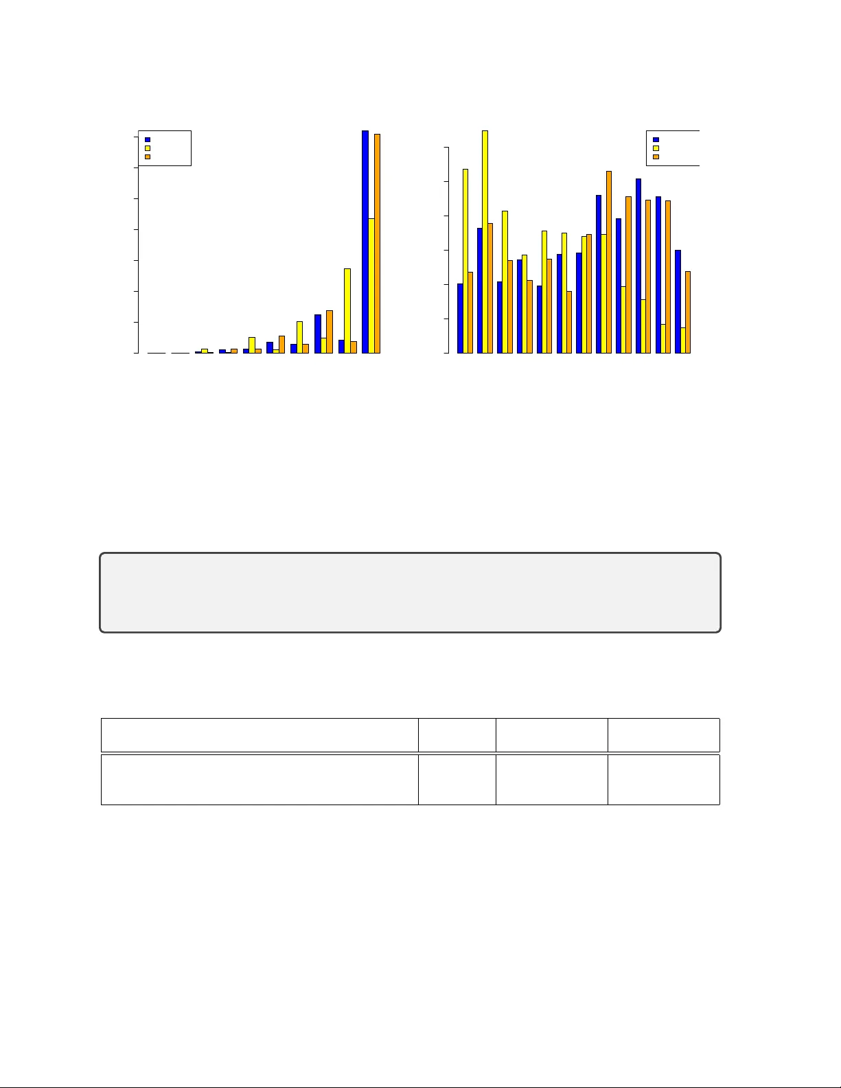
One-Shot Individual Claims Reserving Ronald Ric hman ∗ Mario V. W ¨ uthric h † V ersion of Marc h 13, 2026 Abstract Individual claims reserving has not y et b ecome established in actuarial practice. W e attribute this to the absence of a satisfactory metho dology: existing approac hes tend to b e either o verly complex or insufficien tly flexible and robust for practical use. Building on the classical c hain-ladder (CL) method, w e in tro duced a new persp ective on individual claims reserving in Richman and W ¨ uthric h []. This manuscript has spark ed considerable discussion within the actuarial communit y . The aim of the present pap er is to contin ue and deep en that discussion, with the ultimate goal of adv ancing to w ard a new standard for micro-lev el reserving. Keyw ords. Claims reserving, c hain-ladder method, individual claims reserving, micro-level reserving, gran ular reserving, neural net w orks, Mac k’s metho d. 1 In tro duction W e recently uploaded an individual claims reserving prop osal to arXiv:2602.15385 that ad- dressed many of the shortcomings presen t in the published micro-reserving literature; see Rich- man–W ¨ uthric h [10]. Starting from the classical chain-ladder (CL) method of Mack [8], we deriv ed an alternativ e represen tation of the ultimate claim predictor. This alternativ e represen- tation motiv ates a direct estimation of pro jection-to-ultimate (PtU) factors which allo w for a one-shot for e c ast of the ultimate claims. The approach extends naturally to individual claims reserving for rep orted but not settled (RBNS) claims, allowing one to incorp orate arbitrary input information (including dynamic sto chastic cov ariates) into the estimation procedure of individual RBNS claims reserv es. Our arXiv paper has stimulated substantial discussion of the prop osed approac h, indicating that this ma y b e a promising wa y forward for individual claims reserving. It has also b een noted that our main CL result is not new, it had previously appeared in the literature by Lorenz– Sc hmidt [5]. The purp ose of the present manuscript is to address the man y p oints raised in these discussions and to examine the op en issues identified, we also refer to Richman–W¨ uthrich [10, Section 5] for a list of p oten tial next steps. W e b egin b y summarizing some of the feedback receiv ed; an ac kno wledgemen t is found at the end of this section. ∗ insureAI, ronaldric hman@gmail.com † Departmen t of Mathematics, ETH Zurich, mario.wuethric h@math.ethz.ch 1 • “Ma yb e I am confusing the metho ds here but for triangles y our PtU factors are called grossing-up factors, could that b e? (b ecause I think this recursiv e tec hnique was already used for triangles in the grossing-up metho d of (Handb o ok of Loss Reserving, Radtk e, p 127))?”; commen t b y Florian Gerhardt. This is indeed correct – thank you! W e were not aw are of the corresp onding result of Lorenz– Sc hmidt [6, page 130]; in fact, this CL result w as first published by the same authors [5] in 1999. F ollowing their theorem in Lorenz–Schmidt [6, page 130], the authors state “..., the grossing up metho d is irrelev ant in practice.” W e b eliev e that this assessment is to o p essimistic in the era of mac hine learning. In our view, precisely this structural p ersp ectiv e provides the key to bringing individual claims reserving in to practical applications. This is also supp orted by the following commen ts that w e receiv ed: • “Y our comment ’An alternative of building full simulation mo dels for complex claims pro cesses with multiple sto chastic cov ariates and nested pro jections is not very practical’ is in teresting – this is basically what I w as working on at the start of m y career! Admittedly without a lot of the complexity y ou could build into it, b ecause it w as to o computationally in tensiv e bac k then. But I’m not at all con vinced it’s impractical now adays.”; comment b y Chris Dolman. • “I exp erimen ted with a similar idea sev eral years ago and a couple of clients reported bac k that it work ed well. They kept their existing triangle metho ds to keep the regulator happ y but used the individual claim ultimate cost machine learning approac h to inform the triangle parameters.”; commen t b y Colin Priest. • “I’v e w ork ed on something very similar t w o y ears ago. I called it ’Similarity score weigh ted micro chain ladder’. It also had the same recursive pattern, but predictions of the p oin t to ultimate estimates p er claim were made with simple classification techniques to estimate distance measures b etw een the claim to predict with older claims to take a weigh ted a v erage p oin t to ultimate (as opp osed to using a NN for this as in your case). It b ecomes computationally complex really quic kly . One thing I found quite useful for computational efficiency here was to group claims in op erational time bands instead of developmen t p erio ds. This works esp ecially w ell if y ou hav e transaction dates in y our data. In this w ork we w ere sp ecifically lo oking to close the gap b et w een micro reserving and triangle reserving since adoption of micro reserving has b een so p o or. Great to see you guys also mo ving in to this space.”; commen t b y Stephan Marais. • “W ondering if it’s the same idea as in the addendum [to Semenovic h [12]]? This is some- thing I lo ok ed into originally 10+ years ago. But nev er got to a satisfactory formulation around doing join t IBNR and IBNER estimation in a single regression mo del un til the metho d in the addendum.”; commen t b y Dimitri Semeno vic h. • “Did something similar to estimate prob default after 12 months in IFRS9 ...”; comment b y Willem Ras. • “This is really in teresting work. I think micro reserving is the next step in reserving, not just for improv ed accuracy , but also for greater flexibility . As so on as data is compressed 2 in to a triangle, m uch of the claim-level information is lost. P arodi’s triangle-free pap er [9] makes this p oint nicely with the analogy of moving from a high-resolution to a low- resolution picture. W orking at claim level makes it easier to reflect environmen tal shifts, suc h as inflation sho c ks, detect c hanges in business mix earlier or generate different views since IBNR is pro duced from b ottom-up. But triangles hav e survived for nearly a cen tury for a reason: they are simple, robust, and hard to fo ol. So I exp ect they will stick around for the foreseeable future.”; commen t b y Claudio Reb elo. The ab o ve feedback is v ery exciting, and it seems that man y colleagues hav e been considering suc h or a similar approach. W e see our first main con tribution in do cumenting all these similar though ts and in making the link to the PtU factors in a CL context, whic h turned out to b e the grossing-up metho d of Lorenz–Schmidt [6]. Concerning the last remark, (individual) claims reserving data has a natural triangular structure through censoring at the present ev aluation date. The present pap er illustrates ho w triangular metho ds on aggregated data can b e refined to b e able to op erate on individual claim-level information. There were t w o main critical p oints raised ab ov e: the computational side (whic h indeed may b e demanding) and the recursive structure (whic h ma y b e prone to biases). W e will come bac k to these issues in the next bullet p oints and in our numerical studies b elow. The prop osal in the addendum to Semenovic h [12] starts from a cross-classified Poisson mo del, whic h provides a different wa y of computing the CL reserv es; see Hac hemeister–Stanard [2], Kremer [3] and Mac k [7]. This cross-classified structure presents a more restrictiv e mo del from a mathematical p ersp ectiv e, but from a computational viewp oint it circumv en ts the recursive estimation and forecast structure. This indeed ma y pro vide another very promising alternative, i.e., by solving the mo del es timation by a single maximum likelihoo d estimation (MLE) pro cedure. • “The approach is v ery interesting and promising, esp ecially , b ecause it do es not propose another ML approach, but it is rather thinking ab out restructuring the data to preform individual claims reserving.”; commen t b y Christian Loren tzen. • “Wh y don’t you start with a GLM instead of the neural netw ork?”; comment b y Christian Loren tzen. • “Sounds interesting. Certainly jumping to ultimate is more interesting and aligned with UW views on v ariability . Do es the mo del allow one / n -time step forward pro jections? Helps S2 rep orters with MVM calcs.”; comment by David Menezes. • “Curious what the adv antage is ov er just building a GBM that samples ov er the future space for the underlying data and uses the length of the forecast horizon as one of the inputs?”; commen t b y Alex Ro wley . • “Nice approach for RBNS under CL! Being a fan of generic ligh t w eigh t neural mo dels, I recommend exploring an additional path wa y , further relaxing mo del assumptions: the use of a (neural) contin uous time-to-even t framework including in terv al censoring. In this con text IBNR and RBNS can b e in terpreted as in termediate states b etw een claim o ccurrence and final settlement. The entire sto c hastic claim pro cess then b ecomes fully explicit, with simulation as the to ol for deriving all estimates.”; comment b y Anne v an der Sc heer. 3 The first item of the ab o v e list is a p erfect summary of our in ten tion, i.e., it is not ab out a specific mo del architecture, but rather ab out ho w to organize the data. The second item, starting with a generalized linear mo del (GLM), is an excellent prop osal that w e should already ha v e considered in our first pap er [10]. Ultimately , any reasonable regression mo del may w ork, the s pecific choice will dep end on its purp ose, see Shmueli [13] on ‘T o explain or to predict?’, e.g., for cash flow forecasting or mid-year reserving transformer deco ders could b e useful to ols. Ho w ev er, the prop osal of starting with a GLM is a v ery v alid one, and one of the exciting findings of the presen t case study is that even a linear regression mo del do es an excellent job! The linear regression can b e computed v ery efficiently , and therefore, we can even build on an individual claims b o otstrap algorithm here to assess mo del uncertaint y . If we understand correctly , the last tw o items of the ab o v e list are related to the addendum of Semenovic h [12] who prop osed a cross-classified Poisson mo del that can simultaneously deal with incurred but not rep orted (IBNR) and RBNS claims. Using the cross-classified Poisson structure, the problem can be solv ed in closed-form using MLE. F or more complex architectures, this seems less clear. As explained in our previous pap er [10], we rather prefer to circumv ent a sim ulation extrap olation as this is a topic with its own difficulties. Adding the length of the forecast horizon may b e an interesting prop osal to shrink the num b er of necessary regression mo dels. How ev er, at the current stage, it seems not fully aligned with our recursive structure of estimating the PtU factors. • “One mo del p er accident p erio d seems a lot.” • “Can this also b e used for quarterly (mid-year) reserving?” • “It would be nice to hav e a simple IBNR mo del to b e able to compare the results to classical CL.” W e agree that computationally one mo del p er accident/dev elopment p erio d can b e demanding. Ho w ev er, this is not an y differen t from the CL metho d b ecause each CL factor needs to b e in terpreted as ’one mo del’ in this set-up: note that eac h CL factor solves a regression problem (without an in tercept). In the presen t pap er, we solve everything with linear regression mo dels whic h can b e computed v ery efficien tly . It allows for quarterly reserving. In fact, the input can b e in con tin uous time, ev en if the predic- tion is only on an ann ual grid. After year 2000, when many insurance companies transitioned from ann ual to quarterly rep orting, they initially used a grossing-up metho d to complete a partially observed calendar year to receive an end-of-year forecast. Based on this end-of-year forecast they p erformed a CL or Bornhuetter–F erguson [1] metho d on an annual grid. Finally , incurred but not rep orted (IBNR) claim forecasting is a crucial missing piece in our previous w ork, Ric hman–W ¨ uthric h [10], whic h w e are going to tackle in Section 6, b elo w. Organization of this manuscript. • Section 2 revisits the classic CL metho d. W e discuss the transition from the iterative one-p erio d ahead roll-forward extrap olation metho d to recursive one-shot ultimate claim prediction using the PtU factors. T ypically , this is done on aggregated cumulativ e pay- men ts, and we explain its decomp osition to individual claims observ ations. This pa v es the path to b ootstrapping individual claims histories, and we c hallenge Mack’s [8] mo del error estimate b y a corresp onding individual claims history b o otstrap analysis. 4 • In Section 3, we distinguish claims according to their rep orting status – resulting in RBNS and IBNR claims. This is a crucial step in individual claims reserving to ensure that PtU factors are estimated on consistent claims cohorts – this is the first step that significantly differs from CL reserving on aggregated claims, and it is the crucial step to prepare for individual claims reserving. This step also provides a no vel decomp osition of the classical CL reserv es in to RBNS reserv es and IBNR reserv es. • Section 4 is our core section. W e div e into individual claims reserving for RBNS claims, and interestingly , we see that a linear regression mo del on the individual claim features can attain an excellen t predictiv e p erformance. – Section 4.1 presents the generic recursiv e one-shot PtU forecast algorithm for RBNS claims. This is our core to ol for individual claims reserving; see Algorithm 3. – Section 4.2 gives the first real data application of Algorithm 3. This application is fully based on linear regression mo dels (and a Marko v assumption). – Section 4.3 applies an individual claims history b o otstrap to the previous individual claims reserving metho d. This can b e done efficiently b ecause all predictive mo dels are based on linear regressions. – Section 4.4 c hallenges the linear regression mo dels with neural netw orks, with the result that the net w orks do not pro vide a significan tly b etter predictiv e result. – Section 4.5 analyzes transformer arc hitectures to see whether w e can gain predictiv e p o w er by inputting the entire past claims history (by dropping the Marko v assump- tion). In our small-scale example, the answer is negative, but this should b e recon- sidered on bigger datasets to receive b etter answ ers, i.e., this section rather provides a pro of of concept in the sense that transformers can b e in tegrated into the forecast pro cedure, and they pro vide stable results. • In Section 5, w e analyze the predictiv e p ow er of claims incurred information. Our finding is that on a (small) liability insurance dataset, the claims incurred information gives more accurate forecasts than the individual cumulativ e paymen t information, in particular, in com bination with the claims status information. • In Section 6, we discuss setting the IBNR reserv es for late rep orted claims. This is p er- formed b y a simple CL application on the predicted ultimates of RBNS claims. • Section 7 concludes and giv es an outlo ok. Ac kno wledgemen t. Thank you v ery m uch for the n umerous and very useful feedbac k (in alphab etical order): Chris Dolman, Florian Gerhardt, Sy ed Kirmani, Christian Lorentzen, Stephan Marais, David Menezes, Colin Priest, Willem Ras, Claudio Reb elo, Alex Rowley , Dim- itri Semeno vic h, Anne v an der Sch eer. 2 Chain-ladder metho d - revisited W e b egin b y revisiting Mac k’s [8] CL algorithm and its reform ulation that leads to the app ealing structure for individual claims reserving using mac hine learning (ML) metho ds. This giv es us 5 the motiv ation and the basis for all subsequent deriv ations; for full technical details w e refer to Ric hman–W ¨ uthric h [10]. 2.1 Chain-ladder algorithm - recursiv e one-shot forecast This section presen ts the step going from the one-p erio d ahead roll-forward CL extrap o- lation to the recursive one-shot ultimate claim forecast. F or this w e define the PtU factor that allo ws one to gross-up the last observ ed cum ulativ e pa yments. W e consider I acciden t p erio ds and a maximal dev elopment delay J , throughout J < I . Cum ula- tiv e paymen ts for the claims in acciden t p erio d i ∈ { 1 , . . . , I } at developmen t delay j ∈ { 0 , . . . , J } are denoted b y C i,j , and w e assume that these cumulativ e paymen ts are strictly p ositive for all indexes ( i, j ); cumulativ e pa yments C i,j means that these v ariables collect all the pa ymen ts made for acciden t y ear i within the dev elopmen t p erio ds up to p eriod j . A t calendar time I , we hav e observed the upp er triangle/trap ezoid D I = { C i,j ; i + j ≤ I , 1 ≤ i ≤ I , 0 ≤ j ≤ J } , (2.1) this corresp onds to the green triangles in Figures 1 and 2. The general goal is to predict the ultimate c laims C i,J for all accident p erio ds i with i + J > I , i.e., the accident p erio ds that are not fully dev elop ed at time I . F or the CL reserving metho d, w e estimate the so-called CL factors ( f j ) J − 1 j =0 at time I b y b f CL j = P I − ( j +1) i =1 C i,j +1 P I − ( j +1) i =1 C i,j . (2.2) The CL pr e dictors at time I of the ultimate claims for acciden t p eriods i > I − J are defined by b C CL i,J = C i,I − i J − 1 Y j = I − i b f CL j ; (2.3) these are the classic CL predictors; see Mack [8]. Define the pr oje ction-to-ultimate (PtU) factors b F CL j = J − 1 Y l = j b f CL l for j ∈ { 0 , . . . , J − 1 } . (2.4) These giv e the iden tical CL predictors for i > I − J b C CL i,J = C i,I − i J − 1 Y j = I − i b f CL j = C i,I − i b F CL I − i . (2.5) In the actuarial literature, the PtU factors (2.4) are also called gr ossing-up factors , making the reserving metho d in (2.5) a grossing-up reserving metho d; see Lorenz–Schmidt [6]. The mechanics of the CL estimation and prediction pro cedure (2.3) is illustrated in Figure 1. It has the follo wing iterativ e one-p erio d ahead roll-forward structure b C CL i,J = C i,I − i J − 1 Y j = I − i b f CL j = C i,I − i · b f CL I − i | {z } I − i → I − i +1 · b f CL I − i +1 | {z } I − i → I − i +2 · . . . · b f CL J − 1 . 6 Figure 1: One-perio d ahead roll-forward extrap olation to predict the ultimate claims C i,J using the observ ations C i,I − i , i > I − J , at time I (for I = 7 and J = 6); this figure is taken from [10]. It is precisely this iterativ e one-p erio d ahead roll-forw ard extrap olation structure that p oses significan t difficulties in individual claims reserving using ML metho ds b ecause dealing with suc h extrap olations of sto chastic pro cesses is generally a difficult problem. This has led to the idea of trying to p erform a direct one-shot for e c ast of the ultimate claim by dir e ctly estimating the PtU factor, where ’directly estimating’ means that we do not go through the iterative one- p erio d ahead construction (2.4), but we directly estimate the PtU factor in a single computation, see (2.6). As pro v ed in Lorenz–Schmidt [6] and verified in Richman–W¨ uthrich [10, Prop osition 2.2], this is p ossible. Algorithm 1 gives this one-shot prediction v ariant of the CL predictors (2.3); for mathematical details see Richman–W¨ uthric h [10, Prop osition 2.2], and it is illustrated in Figure 2. Algorithm 1 Recursiv e one-shot CL prediction algorithm. (a) Initialization for j = J . F or the fully settled accident p erio ds i ∈ { 1 , . . . , I − J } , initialize the algorithm b y b C CL i,J = C i,J . (b) Iter ation j → j − 1 ≥ 0 . Compute recursiv ely b F CL j − 1 = P I − j i =1 b C CL i,J P I − j i =1 C i,j − 1 and b C CL I − ( j − 1) ,J = C I − ( j − 1) ,j − 1 b F CL j − 1 . (2.6) Remark, the predictors (2.6) and (2.3) are iden tical; see Richman–W¨ uthrich [10, Prop osition 2.2]. That is, (2.6) gives a different represen tation of (2.3) which is more app ealing in individual claims reserving. 2.2 Individual claims - a v ailable data This section introduces the individual claims and their individual claim histories. W e dis- tinguish b et w een cumulativ e claims and aggregated claims, and w e explain the difference b et w een RBNS and IBNR claims. The cumulativ e pa ymen ts C i,j consider aggregated pa ymen ts ov er al l claims ha ving o ccurred in acciden t p erio d i up to developmen t p erio d j . W e emphasize that we distinguish the meanings • of cumulative referring to summing pa ymen ts o v er dev elopment p erio ds j , and 7 Figure 2: Bac kw ard (in time) one-shot predictions of the ultimate claims C i,J , i > I − J , using the ‘directly estimated’ PtU factors ( b F CL j ) J − 1 j =0 giv en in (2.6): (left-middle-right) corresp ond to j − 1 = J − 1 = 5, j − 1 = 4 and j − 1 = 3; this figure is tak en from [10]. • of aggr e gate d referring to summing ov er different individual claims. W e no w shift our focus to individual claims mo deling. Assume there are N i claims that occurred in acciden t p eriod i . W e lab el these claims by ν = 1 , . . . , N i , and we study each of these claims individually . Denote the r ep orting delay of the ν -th claim of accident p erio d i by T i | ν ≥ 0; the rep orting delay is the time difference b etw een the o ccurrence p erio d i of the claim and its rep orting (notification) p erio d i + T i | ν at the insurance company . Thus, after rep orting dela y j , all claims ν with rep orting delay T i | ν ≤ j are rep orted at the insurance company , and the claims ν with T i | ν > j are not rep orted at time i + j . F or a fixed time p oin t I , called evaluation date , we hav e the following tw o classes of claims: • w e call the claims that are not rep orted y et, i + T i | ν > I , incurr e d but not r ep orte d (IBNR) claims, and • all other claims, i + T i | ν ≤ I , are called r ep orte d but not settle d (RBNS) claims. By con v en tion, RBNS claims include al l rep orted claims, these can b e open or closed (settled), as some closed claims may require a re-op ening due to late unexp ected further claim dev elopmen ts. As so on as a claim ν is rep orted (RBNS), the insurance company starts to collect information ab out this sp ecific claim. E.g., the insurance company can study its individual cumulative p ayment pr o c ess giv en b y C i, 0: J | ν = h C i, 0 | ν 1 { T i | ν ≤ 0 } , C i, 1 | ν 1 { T i | ν ≤ 1 } , . . . , C i,J | ν 1 { T i | ν ≤ J } i . (2.7) W e mask C i,j | ν = 0 all IBNR p erio ds j < T i | ν , i.e., b efore the claim has b een rep orted to the insurance compan y; one could also use an y other mask v alue. A lo wer index 0: J generically denotes a sequence that considers the time indexes j = 0 , . . . , J . The aggr e gate d cumulativ e paymen ts C i,j o v er all claims that hav e o ccurred in accident p erio d i up to dev elopmen t p erio d j are then computed b y C i,j = N i X ν =1 C i,j | ν 1 { T i | ν ≤ j } = X ν : T i | ν ≤ j C i,j | ν , (2.8) 8 Figure 3: (lhs) Individual cumulativ e pa ymen ts C i,j | ν in the upp er triangle i + j ≤ I (eac h row is one claim, p erio d i = 4 has twice as man y claims as i = 3), and (rhs) aggregated cumulativ e claims C i,j in the upp er triangle. Late rep ortings are illustrated by gra y bars in the left-hand side figure. w e are going to use the latter notation as it is more con v enien t. Naturally , but imp ortantly for the further understanding, only RBNS claims can hav e paymen ts, this motiv ates the expression C i,j | ν 1 { T i | ν ≤ j } in (2.7) and (2.8). Figure 3 (lhs) indicates individual cumulativ e paymen t histories C i, 0 | ν , . . . , C i,I − i | ν in the (ob- serv ed) upp er triangle – each row corresp onds to one claim. The gra y bars show late rep orted claims, e.g., in the first accident p erio d i = 1, there is one claim with rep orting delay T 1 | ν = 2. Suc h claims with a rep orting lag of 2 p erio ds are missing for the most recen t accident p erio ds i = 6 , 7, b ecause they are not rep orted y et, i.e., they are IBNR claims at the ev aluation date I = 7. The right-hand side of Figure 3 shows its aggregated version C i, 0 , . . . , C i,I − i , see (2.8), where all the pa ymen ts are aggregated within acciden t p erio ds i and developmen t p erio ds j . The individual pa ymen t information (2.7) is sufficien t to compute the CL predictors (2.3). How- ev er, often there is additional individual claim information av ailable. W e denote the pro cess of the additional individual information b y X i, 0: J | ν = h X i, 0 | ν 1 { T i | ν ≤ 0 } , X i, 1 | ν 1 { T i | ν ≤ 1 } , . . . , X i,J | ν 1 { T i | ν ≤ J } i , (2.9) where we again use a mask for X i,j | ν for all IBNR p erio ds j < T i | ν , this corresp onds to the gray bars in Figure 3 (lhs). Th us, each claim ν = 1 , . . . , N i of accident p erio d i is describ ed by a claim settlement pr o c ess ( individual claim history ) C i | ν = ( C i, 0: J | ν , X i, 0: J | ν ) . (2.10) The claim settlement comp onents ( C i,j | ν , X i,j | ν ) b efore rep orting j < T i | ν are masked as IBNR p erio ds, and at the ev aluation date I the en tries with indexes i + j > I ha v e not b een observ ed y et, b ecause they lie in the future at time I (this is the lo w er (white) triangle in Figure 3). 9 The additional claim features collect an y information ab out the individual claim, e.g., X i,j | ν =             rep orting dela y T i | ν business line claims t yp e settlemen t dela y j claim status closed/op en at delay j claims incurred at dela y j case reserv es at dela y j             . (2.11) The first three entries are static c ovariates that b ecome av ailable at rep orting, the fourth com- p onen t is a deterministic dynamic c ovariate (it is dynamic but p erfectly predictable), and the last three en tries are sto chastic dynamic c ovariates . The information in (2.11) is called tabular, b ecause it considers structured data that has a tabular form. How ev er, the algorithms presen ted b elo w can also deal with unstructured data, e.g., we could include a medical rep ort into X i,j | ν – medical rep orts are also of sto chastic dynamic nature. F or the CL metho d, we started from a fixed time grid, e.g., a monthly , quarterly or an ann ual grid, with acciden t p erio d index i and developmen t dela y index j living on that grid. The algorithms presen ted b elo w can also deal with con tin uous time inputs. In that case, w e replace the discrete time v ersion (2.10) b y C i | ν = ( C i,t | ν , X i,t | ν ) t ∈ [0 ,J ] , (2.12) that is, we keep a discrete time grid for the acciden t p erio d i , but the claim settlement pro cess liv es in con tinuous time t ∈ [0 , J ]. W e k eep the discrete time in the acciden t p erio d i b ecause the algorithms will b e recursive in that time index. 2.3 Chain-ladder algorithm on individual claims This section discusses the computation of the CL factors being ratios of tw o claim cohorts that are not fully consisten t. This precisely motiv ates the step going from total claims reserv es to RBNS claims reserves. Moreov er, w e represen t the CL factor computation as a minimization problem, whic h is the k ey to lift the CL factors to regression functions. The CL algorithm has b een computed on aggregated cumulativ e paymen ts C i,j . Naturally , w e can p erform the same computations on individual claims. In view of (2.8), the CL factors computed in form ula (2.2) are equally obtained b y b f CL j = P I − ( j +1) i =1 P ν : T i | ν ≤ j +1 C i,j +1 | ν P I − ( j +1) i =1 P ν : T i | ν ≤ j C i,j | ν . (2.13) There are tw o points b eing w orth to b e raised in this alternative representation. These tw o p oin ts are going to b e crucial for our further discussion and understanding. (1) The first p oin t is that the nominator and the n umerator of (2.13) do not consider the iden tical claim cohorts. The difference precisely concerns the claims with rep orting dela y T i | ν = j + 1. 10 This can b e seen as follows b f CL j = P I − ( j +1) i =1 P ν : T i | ν ≤ j C i,j +1 | ν + P I − ( j +1) i =1 P ν : T i | ν = j +1 C i,j +1 | ν P I − ( j +1) i =1 P ν : T i | ν ≤ j C i,j | ν . (2.14) That is, the CL factors include a margin for late rep orted (IBNR) claims – second term in the n umerator of (2.14) – and therefore these factors cannot serv e as predictors on individual RBNS claims b ecause they will lead to biased estimates on these individual RBNS claims, the total bias b eing of the size of the predicted IBNR claims. T o prop erly account for this, w e are going to mo dify the CL metho d in Section 3, b elow. Figure 4: Individual RBNS vs. IBNR pro jection. Figure 4 illustrates this issue for developmen t step j = 2 → j + 1 = 3. If we wan t to extrap olate the RBNS claims of accident p erio d i = 5, the CL factor should only contain the ratio of claims that hav e b een rep orted at settlement delay j = 2. In Figure 4, this is not the case: there is one claim ν of accident p erio d i = 2 with rep orting delay T i | ν = j + 1 = 3 (gray bar). Therefore, the columns for j = 2 and j + 1 = 3 do not contain the identical claims, and the corresp onding CL ratio (2.14) accoun ts for this IBNR claim as w ell. (2) The second p oint we wan t to emphasize is that the estimator (2.13) can b e receiv ed as the solution of a weigh ted square minimization problem. On aggregated claims, this is related to the v ariance assumption in Mack’s [8] distribution-free CL mo del. On individual claims, this needs some care. A t the moment, (2.14) contains IBNR claims at developmen t dela y j b eing mask ed b y zero, but it also contains RBNS claims that ma y hav e individual cumulativ e pa yments C i,j | ν ≥ 0 that are equal zero. That is, on aggregated cumulativ e claims C i,j w e ha ve made the assumption of strict p ositivity , see Section 2.1, but on individual cum ulative claims C i,j | ν w e do not wan t to mak e this assumption as for quite some of these claims the pa yments may only o ccur later. T o cop e with this problem in the estimation pro cedure, we select a small p ositive constan t ϵ > 0, and consider the weigh ted square minimization problem b f ϵ j = arg min f j    I − ( j +1) X i =1 X ν : T i | ν ≤ j +1 max { C i,j | ν , ϵ }  C i,j +1 | ν max { C i,j | ν , ϵ } − f j  2    , (2.15) 11 where w e impute ϵ for non-p ositiv e and IBNR claims T i | ν = j + 1 at settlemen t dela y j . The solution to (2.15) is giv en b y b f ϵ j = P I − ( j +1) i =1 P ν : T i | ν ≤ j +1 C i,j +1 | ν P I − ( j +1) i =1 P ν : T i | ν ≤ j +1 max { C i,j | ν , ϵ } ≤ b f CL j with b f ϵ j ↑ b f CL j for ϵ ↓ 0. (2.16) This shows that we can estimate the CL factors from minimization problems. This observ ation is the k ey to lift CL reserving to ML metho ds, namely , f j = f j ( C i, 0: j | ν , X i, 0: j | ν ) in (2.15) can b e made dep enden t on claim cov ariates ( C i, 0: j | ν , X i, 0: j | ν ), which op ens to do or for regression mo deling of the CL factors. Belo w, w e are going to mo dify this in three wa ys: (1) W e will use the one-shot ultimate claim forecast v arian t as outlined in Algorithm 1. This will a v oid complicated iterativ e one-step ahead extrap olations. (2) W e will ensure that the claim cohorts considered in the nominator and n umerator in (2.13) are identical, so that the metho d is suitable for individual RBNS claim prediction without adding a margin for IBNR claims. IBNR claims require a separate treatment. (3) W e will consider alternative ob jectiv e functions b ecause optimizing (2.15) on individual claims and for flexible regression functions f j ( C i, 0: j | ν , X i, 0: j | ν ) ma y result in stabilit y issues, caused b y non-p ositiv e (or small) individual cum ulativ e claims C i,j | ν . Remarks. Making the CL factors f j ( C i, 0: j | ν , X i, 0: j | ν ) co v ariate-dep enden t has already b een considered in W ¨ uthric h [14]. This reference used a one-step ahead roll-forward extrap olation similar to (2.3), resulting in the same difficulties as many other prop osed metho ds in the litera- ture. Another interesting v ariant is that we could replace the weigh ts of IBNR claims in (2.15) b y (premium) exp osures giving us a t yp e of incremental loss ratio metho d for IBNR claims. 2.4 Lab: Chain-ladder reserving and individual b o otstrap This section presents our tw o running examples (accident insurance and liabilit y insur- ance) that will b e revisited throughout the do cument. W e compute their CL reserves, Mac k’s prediction uncertaint y estimates, and w e benchmark Mack’s mo del error estimates b y individual claims history b o otstrap estimates, see T able 3. In this do cumen t, we study tw o small-scale examples. These small-scale examples provide a pro of of concept, and generalization to bigger datasets still needs to b e confirmed. T o b e able to p erform a prop er pro of of concept, we select comparably old data such that not only the upp er triangles are observed, but in these tw o datasets also the low er triangles are kno wn. Thus, an y metho d that we dev elop on the upp er triangle can b e b enchmark ed against the ground truth in the low er triangle in our tw o examples. Of course, this is very useful for providing evidence that our prop osals work; generally , the results that require knowledge of the low er triangle are earmark ed b y an upp er index ‡ in this do cument, see, e.g., T able 3, below. W e start by presenting the tw o datasets, these are the same as in Richman–W¨ uthrich [10], and we also cop y-paste the explaining text from that reference to describ e the data. 12 2.4.1 Acciden t insurance data The first dataset considers accident insurance on an ann ual scale with 5 fully observ ed accident y ears, i.e., w e hav e a fully observ ed 5 × 5 square. F or mo del fitting and forecasting, w e only use the upp er triangle , as in Figure 2, and we b enchmark the forecasts against the true ultimates whic h are a v ailable here (having also observ ed the lo wer triangle). Characteristic Time scale calendar y ears Num b er of acciden t years 5 Num b er of dev elopment years 5 Num b er of rep orted claims 66,639 Data description Ann ual individual cumulativ e paymen ts C i,j | ν Claim status O i,j | ν ∈ { 0 , 1 } for closed/open at the end of p erio d j Binary static cov ariate for work or leisure acciden t Calendar mon th of accident occurrence Rep orting dela y in daily units T able 1: Characteristics of acciden t dataset. T able 1 shows the a v ailable data. There are 66,639 rep orted claims with a fully observed de- v elopmen t history ov er the 5 × 5 square. Besides the individual cumulativ e paymen t pro cess C i, 0:4 | ν , there is information ab out the claim status pro cess O i, 0:4 | ν , with O i,j | ν = 1 meaning that the ν -th claim of accident year i is op en at the end of settlement dela y j , and closed oth- erwise. Then, there is static information ab out: w ork or leisure related acciden t, the calendar mon th of the accident and the rep orting delay in daily units. F or more information w e refer to Ric hman–W ¨ uthric h [10]. 2.4.2 Liabilit y insurance data The second dataset considers liability insurance. W e again ha v e a fully observ ed 5 × 5 square and for mo del fitting we only use the upp er triangle. Characteristic Time scale calendar y ears Num b er of acciden t years 5 Num b er of dev elopment years 5 Num b er of rep orted claims 21,991 Data description Ann ual individual cumulativ e paymen ts C i,j | ν Claim status O i,j | ν ∈ { 0 , 1 } for closed/open at the end of p erio d j Claims incurred I i,j | ν ≥ 0 Binary static cov ariate for priv ate vs. commercial liability Calendar mon th of accident occurrence Rep orting dela y in daily units T able 2: Characteristics of liabilit y dataset. 13 T able 2 shows the av ailable data of the liability insurance dataset. The main difference to the previous example is that for this dataset there is also a claims incurred pro cess I i, 0:4 | ν a v ailable. The claims incurred pro cess is a claims adjuster’s prediction of the individual ultimate claim that is contin uously up dated when new information arrives, i.e., this is a sto chastic process driv en b y the claims adjuster’s assessmen ts. 2.4.3 Mac k’s c hain-ladder metho d and individual b o otstrapping W e start with Mack’s [8] distribution-free CL metho d. It allows one to compute the CL reserv es at the ev aluation date I for eac h accident y ear i > I − J , giv en by b R CL i = b C CL i,J − C i,I − i . These CL reserv es are b enc hmarked against the true outstanding loss liabilities (OLL), given b y OLL i = C i,J − C i,I − i . These true OLL present the ground truth, and they are given in our small-scale examples b ecause we kno w the low er triangles. T able 3 shows the CL results for the t w o datasets summed o ver all accident y ears i , and the column ‘Error ‡ ’ gives the total for e c ast err or I X i = I − J +1 b C CL i,J − C i,J . (2.17) T rue OLL ‡ CL Reserv es Pro c.Unc. Est.Err. RMSEP Error ‡ % RMSEP ‡ Acciden t dataset Mac k’s CL mo del [8] 24,212 23,064 1,429 851 1,663 -1,148 69% Individual b ootstrap 24,212 22,988 – 937 – -1,224 – Liabilit y dataset Mac k’s CL mo del [8] 15,730 11,526 1,383 1,413 1,977 -4,204 213% Individual b ootstrap 15,730 11,531 – 1,201 – -4,199 – T able 3: Mack’s CL results on cumulativ e pa ymen ts and CL results using an individual claims history b ootstrap; the earmarked columns ‡ can only be computed b ecause we know the lo w er triangle in our t w o examples. W e observe that in b oth datasets we underestimate the true OLL by -1,148 and -4,204, resp ec- tiv ely , see column ‘Error ‡ ’ corresp onding to (2.17). T o assess the magnitude of this underesti- mation, w e additionally compute Mack’s [8] ro oted mean squared error of prediction (RMSEP), giv en b y the square ro ot of the conditional MSEP msep P i C i,J |D I  X i b C CL i,J  = E   I X i = I − J +1 b C CL i,J − C i,J ! 2       D I   = V ar I X i = I − J +1 C i,J      D I ! | {z } pr oc ess unc ertainty + I X i = I − J +1 b C CL i,J − E [ C i,J | D I ] ! 2 | {z } estimation err or , where D I refers to the a v ailable cum ulative pa ymen ts at time I , see (2.1). One of the main ac hiev emen ts of Mac k [8] was to compute/estimate the (rooted) pr o c ess unc ertainty (‘Proc.Unc.’; 14 also called irr e ducible risk ) and the (rooted) estimation err or (‘Est.Err.’; also called mo del err or ) under suitable CL assumptions. This then provides the RMSEP . The numerical results are presen ted in columns ‘Pro c.Unc.’, ‘Est.Err.’ and ‘RMSEP’ of T able 3 – we alwa ys sho w the ro oted versions. W e observ e that the forecast error (2.17) makes 1 , 148 / 1 , 663 = 69% of the RMSEP in the accident insurance case, this is a reasonable deviation (less than one RMSEP), and we cannot reject the CL metho d in this case. In the liability insurance case, the CL metho d seems to p erform worse, the forecast error (2.17) makes 4 , 204 / 1 , 977 = 213% of the RMSEP . This ma y lead us to doubt the application of the CL algorithm for the liabilit y insurance data. 1 Next, w e presen t an individual claims history (non-parametric) b o otstrap. In our con text, a non- parametric b o otstrap is useful to assess the (ro oted) estimation error ‘Est.Err.’, i.e., it is useful to analyze the mo del estimation uncertaint y term b y re-sampling new upp er triangles to ev aluate the resulting fluctuations in the CL factor estimates. It is not directly possible to assess the pro cess uncertaint y term with an individual claims history b o otstrap in our set-up. The issue is that only the oldest acciden t p erio ds i ≤ I − J hav e observe d ultimate claims C i,J (last column of upp er triangle/trap ezoid, see Figure 4), and for all other accident p erio ds i = I − J + 1 , . . . , I we cannot re-sample (b o otstrap) ultimate claims. If the ultimate claim observ ations C i,J , i ≤ I − J , are sufficien tly ric h, w e can pro ject those to the more recen t accident p erio ds, otherwise we would not recommend the b o otstrap to assess the process uncertain t y term, but only the (ro oted) estimation error ‘Est.Err.’. The (ro oted) estimation error ‘Est.Err.’ can b e rewritten as I X i = I − J +1 b C CL i,J − E [ C i,J | D I ] = I X i = I − J +1 C i,I − i   J − 1 Y j = I − i b f CL j − J − 1 Y j = I − i f j   . F or the non-parametric b o otstrap, w e randomly draw individual claims C i, 0: I − i | ν = ( C i,j | ν ) I − i j =0 with replacemen t from the upper individual claims triangle, see Figure 4, suc h that the bo otstrap sample has the same size as the original data sample of individual claims – we p erform this dra wing with replacemen t sim ultaneously o ver all acciden t p erio ds i ∈ { 1 , . . . , I } which also in tro duces some volatilit y across the acciden t p erio ds. The resulting b ootstrap sample is used to re-estimate the CL factors – by first aggregating the individual b o otstrapp ed claims similarly to (2.8) resulting in b o otstrapp ed aggregated cumulativ e pa ymen ts C ∗ i,j , i + j ≤ I – and these are then used to compute the estimated b ootstrapp ed CL factors ( b f ∗ j ) J − 1 j =0 similar to (2.2). Then, w e compute the b o otstrappe d ultimate claim predictors by b C ∗ i,J = C i,I − i J − 1 Y j = I − i b f ∗ j , (2.18) note that the basis C i,I − i remains fixed, as this corresp onds to the conditioning on D I in the RMSEP , i.e., we do not re-simulate the last diagonal of the upp er triangle, we only b ootstrap in order to assess the estimation uncertaint y in the CL factor estimates. Rep eating this re- estimation pro cedure man y times, allows us to assess the av erage and the standard deviation in the b ootstrap predictors b C ∗ i,J , the latter b eing an estimation uncertaint y estimate. W e rep ort these b ootstrap results (received from 1,000 b o otstrap samples) on the lines ‘Individual b o ot- strap’ in T able 3. The a v erage b o otstrap prediction is very well aligned with the original CL 1 The RMSEP is on the level of a standard deviation, so we typically chec k whether it exceeds tw o standard deviations (RMSEPs) or not. 15 predictors b C CL i,J , thus, the b o otstrap do es not indicate any bias. The magnitude of the b ootstrap standard deviation aligns w ell with the ro oted estimation error estimate of Mack [8], we hav e a slightly higher v alue in the ac ciden t dataset (937 vs. 851) and a low er v alue in the liability dataset (1,201 vs. 1,413), but o v erall the magnitudes align. In the ab ov e non-parametric b o otstrap analysis, we resample the entire upp er triangle b y drawing with replacemen t. Another interesting analysis w ould b e to re-sample only one selected accident p erio d i , this w ould allo w one to assess the impact of a single at ypical accident p erio d on the en tire claims reserv es. 3 Chain-ladder RBNS reserving In a preliminary step tow ards individual claims reserving, we separate RBNS from IBNR claims. A main motiv ation for this initial step is that there is individual claims information (2.9) av ailable for RBNS claims, and we try to optimally use this information to predict the individual ultimates C i,J | ν of RBNS claims ν , i + T i | ν ≤ I . This is not the case for IBNR claims (b ecause they are not rep orted y et) and only a collectiv e prediction is p ossible, e.g., based on exp osure information. 3.1 Chain-ladder RBNS prediction This section mo difies the recursive one-shot CL prediction algorithm, see Algorithm 1, suc h that it only predicts RBNS claims. This is achiev ed b y considering consistent claim cohorts in extrap olation; s ee Algorithm 2. The CL predictions b C CL i,J co v er b oth the RBNS and the IBNR claims. This comes from the fact that we do not consider the iden tical claims cohorts in the CL factor estimates, the second term in the numerator in (2.14) corresp onds to IBNR claims at dev elopmen t dela y j , see Figure 4. It is straightforw ard to correct for this, and to only consider RBNS claims. W e giv e the one-shot PtU factor v ersion in Algorithm 2, as this is more con v enien t. Algorithm 2 Recursiv e one-shot CL RBNS prediction algorithm. (a) Initialization for j = J . F or the fully settled accident p erio ds i ∈ { 1 , . . . , I − J } , initialize the algorithm b y setting b C RBNS i,J | ν = C i,J | ν for all claims ν = 1 , . . . , N i . (b) Iter ation j → j − 1 ≥ 0 . Compute recursiv ely b F RBNS j − 1 = P I − j i =1 P ν : T i | ν ≤ j − 1 b C RBNS i,J | ν P I − j i =1 P ν : T i | ν ≤ j − 1 C i,j − 1 | ν and b C RBNS I − ( j − 1) ,J | ν = C I − ( j − 1) ,j − 1 | ν b F RBNS j − 1 , (3.1) for all RBNS claims ν at time I , i.e., with T I − ( j − 1) | ν ≤ j − 1. Algorithm 2 only extrap olates RBNS claims, and it do es not add any margins for IBNR claims b ecause the numerator and nominator of the PtU factors b F RBNS j − 1 consider the identic al RBNS claims cohort T i | ν ≤ j − 1 . 16 3.2 Chain-ladder IBNR prediction This section pro vides a partition of the total CL reserv es into RBNS and IBNR reserv es. This is a natural consequence of the recursive one-shot CL RBNS prediction algorithm presen ted in the previous section in Algorithm 2. T o forecast the IBNR claims, w e can pro vide a similar algorithm. The IBNR reserv es will consist of tw o different terms in its estimation: (1) terms stemming from claims that are IBNR at time I , and (2) ultimate claims (estimates) that are used for IBNR prediction, but which are RBNS at time I . F or this reason, the following paragraphs will use b oth upp er indices IBNR and RBNS . Initialize b C RBNS i,J | ν = C i,J | ν for all claims ν = 1 , . . . , N i in accident p erio ds i ∈ { 1 , . . . , I − J } – all these are RBNS claims at time I . The first recursive step J → J − 1 considers b F IBNR J − 1 = P I − J i =1 P ν : T i | ν = J b C RBNS i,J | ν P I − J i =1 P ν : T i | ν ≤ J − 1 C i,J − 1 | ν . (3.2) This giv es the (aggregated) IBNR claim prediction for acciden t p erio d I − ( J − 1) b C IBNR I − ( J − 1) ,J =   X ν : T I − ( J − 1) | ν ≤ J − 1 C I − ( J − 1) ,J − 1 | ν   b F IBNR J − 1 = C I − ( J − 1) ,J − 1 b F IBNR J − 1 . This considers the grossing-up factor from the observ ed cum ulativ e paymen ts C I − ( J − 1) ,J − 1 to the IBNR prediction for accident p erio d I − ( J − 1). This can recursively b e iterated, but the iteration is cum b ersome. E.g., the next step J − 1 → J − 2 lo oks as follo ws b F IBNR J − 2 = P I − ( J − 1) i =1 P ν : T i | ν = J − 1 b C RBNS i,J | ν + P I − J i =1 P ν : T i | ν = J b C RBNS i,J | ν + b C IBNR I − ( J − 1) ,J P I − ( J − 1) i =1 P ν : T i | ν ≤ J − 2 C i,J − 2 | ν . The first term in the numerator corresp onds to the RBNS ultimate claim prediction of claims rep orted with delay T i | ν = J − 1, the second term to the prediction of the claims rep orted with dela y T i | ν = J (all these claims are rep orted at time I ), finally , the last term corresp onds to the IBNR part corresp onding to accident p erio d I − ( J − 1). Th us, we complete the upper- righ t triangle with IBNR predictions, and the missing part of this developmen t rectangle is directly completed with the previous IBNR predictions b C IBNR I − ( J − 1) ,J , so that all IBNR claims in the upp er-righ t square/rectangle are iden tified. A muc h easier wa y to receive the identical result is to subtract the RBNS ultimate claim pre- dictors from the CL ones, that is, for all acciden t p erio ds i > I − J w e hav e b C IBNR i,J = b C CL i,J − X ν : T i | ν ≤ I − i b C RBNS i,J | ν . (3.3) This giv es a simple IBNR predictor for all acciden t p erio ds. Remark. A similar, though different approach is considered in Sc hniep er [11]. The similarity concerns the fact that Schnieper [11] also considers developmen t ratios of type (3.2), how ev er, Sc hniep er [11] uses an external exposure as nominator in (3.2). Extrap olating this in a one- p erio d ahead roll-ov er fashion is then p eformed, this is doable but can b e cumbersome (RBNS 17 CL factors get contaminated b y IBNR parts – though in a mathematically consistent w ay). Ha ving a past cum ulative pa ymen ts nominator and turning the problem to the one-shot ultimate prediction v ersion allo ws us to receiv e an elegan t decomp osition (3.3) in our set-up. 3.3 Lab: Chain-ladder RBNS and IBNR reserving This section provides the example ho w the CL reserves of T able 3 can b e partioned into RBNS reserves and IBNR reserves. This uses the RBNS Algorithm 2 and the decomp o- sition form ula (3.3). W e revisit the tw o examples introduced in Section 2.4. W e apply Algorithm 2 to compute the RBNS reserves. The IBNR reserves are then calculated as the differences (3.3). The results are presen ted in T able 4. T rue OLL ‡ Reserv es RMSEP Error ‡ % RMSEP ‡ Acciden t dataset Mac k’s CL mo del [8] 24,212 23,064 1,663 -1,148 69% RBNS CL prediction, Algorithm 2 19,735 18,959 – -774 – IBNR CL prediction (3.3) 4,478 4,105 – -374 – Liabilit y dataset Mac k’s CL mo del [8] 15,730 11,526 1,977 -4,204 213% RBNS CL prediction, Algorithm 2 11,494 8,601 – -2,893 – IBNR CL prediction (3.3) 4,236 2,925 – -1,311 – T able 4: Mack’s CL results on cum ulativ e pa yments split to RBNS and IBNR reserves; the earmark ed columns ‡ can only b e computed b ecause w e know the low er triangle in our examples. F rom the results in T able 4 w e conclude that the CL metho d on RBNS claims seems to work v ery well for the acciden t insurance dataset. On the liabilit y insurance dataset, the CL metho d seems to b e negatively biased. W e are going to refine this assessment in Section 5, b elo w. W e use the ‘RBNS CL prediction’ results of T able 4 as b enchmarks for all subsequent individual claims reserving metho ds on RBNS claims. 3.4 Individual claims reserving - setting the stage In theory , we are no w fully prepared to dive into individual claims regression mo deling. Ho w ev er, we still wan t to mo dify the w eigh ted square loss minimization problem (2.15) b ecause in fine-grained regression problems, the solutions to the weigh ted square mini- mization may not be v ery robust in case max { C i,j | ν , ϵ } is small. This section introduces an un w eigh ted square loss minimization problem, and we verify that the tw o problems give similar solutions (in the case without cov ariates). W e do this in tw o steps, see Listings 1 and 2. Step 1. T o set the stage for individual claims reserving, we first implement a mo dified version of Algorithm 2. Namely , w e bring the PtU factor es timation in (3.1) in to a regression form so that it in v olv es a w eighted square loss minimization similar to (2.15). 18 Listing 1: Recursive one-shot CL RBNS algorithm with w eigh ted square loss minimization (2.15). 1 # # i n i t i a l i z e u l t i m a t e c l a i m s w i t h o b s e r v e d o n e s f o r a c c i d e n t y e a r s i < = I 0 - J 0 2 c l a i m s $ Y Y < - N A 3 c l a i m s [ w h i c h ( c l a i m s $ A c c D a t e < = I 0 - J 0 ) , ] $ Y Y < - c l a i m s [ w h i c h ( c l a i m s $ A c c D a t e < = I 0 - J 0 ) , ] $ U l t i m a t e 4 5 e p s i l o n < - 0 . 0 0 1 # # a v o i d d i v i s i o n b y z e r o 6 7 # # i t e r a t i v e P t U a l g o r i t h m f o r R B N S p r e d i c t i o n 8 f o r ( j i n r e v ( 0 : ( J 0 - 1 ) ) ) { 9 i < - I 0 - j - 1 10 # # # p r e p a r e l e a r n i n g d a t a f o r G L M 11 s e l e c t < - w h i c h ( ( c l a i m s $ A c c D a t e < = i ) & ( c l a i m s $ R e p D e l a y Y Y < = j ) ) 12 Y Y < - c l a i m s [ s e l e c t , ] $ Y Y # # h a s b e e n f i l l e d i n t h e p r e v i o u s l o o p 13 C C < - p m a x ( e p s i l o n , t r i C C [ s e l e c t , p a s t e 0 ( " X " , j ) ] ) # # t h e s e a r e c u m u l a t i v e c a s h f l o w s 14 l e a r n < - d a t a . f r a m e ( c b i n d ( Y Y , C C ) ) 15 # # # p r e p a r e t e s t d a t a f o r P t U p r o j e c t i o n 16 s e l e c t < - w h i c h ( c l a i m s $ A c c D a t e = = ( i + 1 ) ) 17 Y Y < - c l a i m s [ s e l e c t , ] $ Y Y # # i s N / A 18 C C < - t r i C C [ s e l e c t , p a s t e 0 ( " X " , j ) ] 19 t e s t < - d a t a . f r a m e ( c b i n d ( Y Y , C C ) ) 20 # # # p e r f o r m w e i g h t e d s q u a r e l o s s ( G ) L M - i d e n t i t y - l i n k i s u s e d 21 g l m 1 < - g l m ( Y Y / C C ~ 1 , s t a r t = 0 , w e i g h t s = C C , d a t a = l e a r n , f a m i l y = g a u s s i a n ( ) ) 22 c l a i m s [ s e l e c t , ] $ Y Y < - t e s t $ C C * p r e d i c t ( g l m 1 , n e w d a t a = t e s t , t y p e = c ( " r e s p o n s e " ) ) 23 } Listing 1 reform ulates Algorithm 2 with the PtU factor computation in (3.1) replaced by a linear regression (GLM with iden tit y link) and using a w eigh ted square loss minimization (2.15) for mo del fitting; see line 21 of Listing 1. Since RBNS claims can ha ve individual cum ulativ e pa ymen ts C i,j − 1 | ν b eing equal to zero, w e selected a small p ositiv e constant ϵ = 0 . 001 to a void dividing b y zero, see lines 13 and 21 of Listing 1. The solution of this algorithm giv es the iden tical reserv es as Algorithm 2, up to the ϵ > 0 correction factor, we also refer to (2.16). i T rue OLL ‡ RBNS Algorithm 2 RBNS Listing 1 Error ‡ Ind.RMSE ‡ 1 0 0 0 0 0 2 353 339 339 -14 1.499 3 1,017 1,305 1,305 288 2.956 4 3,102 3,099 3,099 -2 4.263 5 15,263 14,216 14,216 -1,046 8.240 T otal 19,735 18,959 18,959 -774 T able 5: Acciden t insurance: RBNS results of individual claims prediction using Algorithm 2 and Listing 1; the earmark ed columns ‡ use the ground truth in the lo w er triangle. T able 5 verifies that Algorithm 2 and Listing 1 give the same results. The first column shows the true OLL for each accident years i ∈ { 1 , . . . , 5 } . Columns ‘RBNS Algorithm 2’ and ‘RBNS Listing 1’ verify that the t w o algorithms give the same results. The column ‘Error ‡ ’ shows how the total RBNS forecast error of -774 splits across the different accident years i ∈ { 1 , . . . , 5 } , see also second line of T able 4. The final column ‘Ind.RMSE ‡ ’ of T able 5 will be the quan tity of ma jor in terest for all subsequen t mo dels. It considers the ro oted mean square error (RMSE) on an individual claims level , that 19 is, w e define the individual aver age RBNS pr e diction err ors b y Ind.RMSE ‡ i = v u u t 1 P ν : T i | ν ≤ I − i 1 X ν : T i | ν ≤ I − i  b C RBNS i,J | ν − C i,J | ν  2 for i ≥ I − J . (3.4) This is the av erage prediction accuracy on the individual claims level (measured b y the RMSE). T ypically , with improv ed mo dels, we exp ect these num b ers to decrease. Remark that we can compute (3.4) in our examples b ecause we know the low er triangle, earmarked by ‡ . Step 2. Before starting with individual claims reserving, w e still mo dify the algorithm once more. Namely , w e wan t to remov e the weigh ting in the square loss minimization to robustify the prediction algorithm (this also allows us to get rid of the constan t ϵ > 0). F or this, we replace the weigh ted square minimization (2.15) by the following line ar r e gr ession pr oblem for RBNS reserving b ϑ j − 1 = arg min ϑ =( ϑ 0 ,ϑ 1 ) ⊤ ∈ R 2    I − j X i =1 X ν : T i | ν ≤ j − 1  b C i,J | ν −  ϑ 0 + ϑ 1 C i,j − 1 | ν   2    . (3.5) W e add an in tercept ϑ 0 ∈ R and drop the weigh ting (for more robustness). Naturally , this gives a differen t solution. W e v erify in T able 6 that the solution is close to the w eigh ted v ersion. Moreo v er, using the identit y link in the square loss minimization (3.5) implies that the (in- sample) balance prop ert y is fulfilled; see Lindholm–W ¨ uthrich [4]. This is an imp ortan t prop erty that ensures bias con trol in our recursive estimation pro cedure. The co de is provided in Listing 2; and this is the basic co de to dive into regression mo deling for RBNS reserving. Listing 2: Recursive one-shot RBNS reserving algorithm using a Gaussian linear regression (3.5). 1 # # i n i t i a l i z e u l t i m a t e c l a i m s w i t h o b s e r v e d o n e s f o r a c c i d e n t y e a r s i < = I 0 - J 0 2 c l a i m s $ Y Y < - N A 3 c l a i m s [ w h i c h ( c l a i m s $ A c c D a t e < = I 0 - J 0 ) , ] $ Y Y < - c l a i m s [ w h i c h ( c l a i m s $ A c c D a t e < = I 0 - J 0 ) , ] $ U l t i m a t e 4 5 # # i t e r a t i v e P t U a l g o r i t h m f o r R B N S p r e d i c t i o n 6 f o r ( j i n r e v ( 0 : ( J 0 - 1 ) ) ) { 7 i < - I 0 - j - 1 8 # # # p r e p a r e l e a r n i n g d a t a f o r G L M 9 s e l e c t < - w h i c h ( ( c l a i m s $ A c c D a t e < = i ) & ( c l a i m s $ R e p D e l a y Y Y < = j ) ) 10 Y Y < - c l a i m s [ s e l e c t , ] $ Y Y # # h a s b e e n f i l l e d i n t h e p r e v i o u s l o o p 11 C C < - t r i C C [ s e l e c t , p a s t e 0 ( " X " , j ) ] # # t h e s e a r e c u m u l a t i v e c a s h f l o w s 12 l e a r n < - d a t a . f r a m e ( c b i n d ( Y Y , C C ) ) 13 # # # p r e p a r e t e s t d a t a f o r P t U p r o j e c t i o n 14 s e l e c t < - w h i c h ( c l a i m s $ A c c D a t e = = ( i + 1 ) ) 15 Y Y < - c l a i m s [ s e l e c t , ] $ Y Y # # i s N / A 16 C C < - t r i C C [ s e l e c t , p a s t e 0 ( " X " , j ) ] 17 t e s t < - d a t a . f r a m e ( c b i n d ( Y Y , C C ) ) 18 # # # p e r f o r m s q u a r e l o s s ( G ) L M - i d e n t i t y - l i n k i s u s e d 19 g l m 2 < - g l m ( Y Y ~ C C , d a t a = l e a r n , f a m i l y = g a u s s i a n ( ) ) 20 c l a i m s [ s e l e c t , ] $ Y Y < - p r e d i c t ( g l m 2 , n e w d a t a = t e s t , t y p e = c ( " r e s p o n s e " ) ) 21 } T able 6 compares the results of the algorithms given in Listings 1 and 2. This v erifies that the t w o algorithms provide very similar results. W e hav e a preference for the second algorithm, as it is more robust and easy to extend. In fact, this similarit y b etw een the results of Listings 1 20 RBNS RBNS Error ‡ Error ‡ Ind.RMSE ‡ Ind.RMSE ‡ i T rue OLL ‡ Listing 1 Listing 2 Listing 1 Listing 2 Listing 1 Listing 2 1 0 0 0 0 0 0 0 2 353 339 337 -14 -16 1.499 1.489 3 1,017 1,305 1,338 288 321 2.956 2.985 4 3,102 3,099 3,264 -2 163 4.263 4.262 5 15,263 14,216 14,137 -1,046 -1,126 8.240 8.218 T otal 19,735 18,959 19,076 -774 -658 T able 6: Acciden t insurance: RBNS results of individual claims prediction using Listings 1 and 2; the earmark ed columns ‡ use the ground truth in the lo w er triangle. and 2 should b e c heck ed case b y case, and on small p ortfolios with volatile claims it migh t b e violated. W e are now ready: The results of T able 6 serve as b enc hmark for all subsequen t deriv ations on individual RBNS claims reserving (in v olving past claims histories). 4 Individual ultimate prediction - one-shot micro reserving W e now turn our attention to ML applications for individual RBNS claims reserving. F or this w e recall the individual claim settlemen t pro cess (2.10), whic h is giv en b y C i | ν = " C i, 0 | ν X i, 0 | ν ! 1 { T i | ν ≤ 0 } , C i, 1 | ν X i, 1 | ν ! 1 { T i | ν ≤ 1 } , . . . , C i,J | ν X i,J | ν ! 1 { T i | ν ≤ J } # , (4.1) all IBNR p erio ds j < T i | ν are masked, and the p erio ds i + j > I ha v e not b een observed y et, b ecause they lie in the future at the ev aluation date I . Assumption. W e assume that the individual claims pro cesses C i | ν are indep endent, and that they are conditionally i.i.d., giv en the static co v ariates. 4.1 Recursiv e individual RBNS claims reserving This section introduces the generic algorithm for recursive one-shot forecasting using general ML regression mo dels. An imp ortant p oin t is the consistent consideration of past information for estimating and forecasting RBNS claims, see learning sample (4.2). In view of Algorithm 2 and Listing 2, it is obvious how to lift these algorithms to general ML regression mo dels for RBNS reserving. Algorithm 3 gives the generic algorithm. The imp ortan t p oin t is that one alwa ys considers consistent cohorts for PtU factor estimation and pro jection. This is indicated by the choice of the learning sample L j − 1 in Algorithm 3, see (4.2), constraining the inputs b y T i | ν ≤ j − 1 . 21 Algorithm 3 Generic recursive one-shot PtU forecast algorithm for RBNS claims. (a) Initialization for j = J . F or the fully settled accident p erio ds i ∈ { 1 , . . . , I − J } , initialize the algorithm b y setting b C i,J | ν = C i,J | ν for all claims ν = 1 , . . . , N i . (b) Iter ation j → j − 1 ≥ 0 . (b1) Select the learning sample L j − 1 = n b C i,J | ν , ( C i,l | ν , X i,l | ν ) j − 1 l =0  ; T i | ν ≤ j − 1 and i ≤ I − j o . (4.2) (b2) Fit a regression mo del µ j − 1 on the learning sample L j − 1 b y using ( C i,l | ν , X i,l | ν ) j − 1 l =0 7→ µ j − 1  ( C i,l | ν , X i,l | ν ) j − 1 l =0  = E h b C i,J | ν    ( C i,l | ν , X i,l | ν ) j − 1 l =0 i . (4.3) (b3) Compute the predictions of the RBNS claims ν of accident year I − ( j − 1) by b C I − ( j − 1) ,J | ν = µ j − 1  ( C I − ( j − 1) ,l | ν , X I − ( j − 1) ,l | ν ) j − 1 l =0  . (4.4) Remarks 4.1 (Algorithm 3) • Listing 2 is a sp ecial case of Algorithm 3, where the only input information used is the latest individual cum ulativ e pa ymen t, see (3.5). That is, µ j − 1  ( C i,l | ν , X i,l | ν ) j − 1 l =0  = µ j − 1  C i,j − 1 | ν  . (4.5) This mak es it ob vious ho w to lift Listing 2 to a general ML forecast algorithm. • Algorithm 3 describ es one-shot PtU forecasting of RBNS claims. Recursively going from settlemen t p erio d j to p erio d j − 1, we aim at forecasting the RBNS claims of accident p erio ds I − ( j − 1), see (4.4). Since these claims are RBNS claims at time I , they can hav e a maximal rep orting delay of T i | ν ≤ j − 1 . This is then reflected in the learning sample L j − 1 b y setting the corresponding side constrain t, see (4.2). Th us, the learning sample and the forecast problem consider the same side constrain t in building their claims cohorts. • Since we do not know the true ultimate claims C i,J | ν for accident p erio ds i > I − J , we recursiv ely replace them b y their forecasts b C i,J | ν , see (4.2). This is completely analogous to the one-shot RBNS prediction (3.1). Using the tow er prop erty for conditional exp ectation, this is justified as follo ws ( C i,l | ν , X i,l | ν ) j − 1 l =0 7→ µ j − 1  ( C i,l | ν , X i,l | ν ) j − 1 l =0  = E h C i,J | ν    ( C i,l | ν , X i,l | ν ) j − 1 l =0 i = E h b C i,J | ν    ( C i,l | ν , X i,l | ν ) j − 1 l =0 i . The latter can b e learned from the learning sample L j − 1 giv en in (4.2). Recursive iteration completes the forecasting, and it is aligned with Figure 2. • F rom Algorithm 3 it is obvious that this forecast pro cedure can deal with any (dynamic) input information, in particular, w e can also consider contin uous time inputs (2.12) and unstructured data. 22 • In practical applications, the only critical item of this algorithm is its recursive nature. In particular, we need to p erform a careful bias control b ecause a bias can easily propagate through the recursive forecast arc hitecture. In Listing 2 w e consider a Gaussian linear regression problem, and MLE provides the in-sample balance prop ert y , thus, it pro vides an in-sample guarantee of un biasedness. F or more complex ML algorithms we need to enforce this balance prop ert y manually , e.g., by a p ost correction or by regularization, w e come bac k to this in (4.9), b elo w. 4.2 Lab: Acciden t insurance example – linear regression This section giv es first explicit examples of the one-shot PtU forecast Algorithm 3. It uses a (simple) linear rgression on the av ailable cov ariates of the last observ ed p erio d. The first example in T able 7 only considers individual cum ulativ e pa yments and the claim status, the second example in T able 8 considers all a v ailable cov ariates at time j − 1. W e revisit the example of T able 6 and we c hallenge the results by more complex regression mo dels based on Algorithm 3. Listing 3: Recursiv e one-shot PtU RBNS algorithm including the latest claim status. 1 # # i n i t i a l i z e u l t i m a t e c l a i m s w i t h o b s e r v e d o n e s f o r a c c i d e n t y e a r s i < = I 0 - J 0 2 c l a i m s $ Y Y < - N A 3 c l a i m s [ w h i c h ( c l a i m s $ A c c D a t e < = I 0 - J 0 ) , ] $ Y Y < - c l a i m s [ w h i c h ( c l a i m s $ A c c D a t e < = I 0 - J 0 ) , ] $ U l t i m a t e 4 5 # # i t e r a t i v e P t U a l g o r i t h m f o r R B N S p r e d i c t i o n 6 f o r ( j i n r e v ( 0 : ( J 0 - 1 ) ) ) { 7 i < - I 0 - j - 1 8 # # # p r e p a r e l e a r n i n g d a t a f o r G L M 9 s e l e c t < - w h i c h ( ( c l a i m s $ A c c D a t e < = i ) & ( c l a i m s $ R e p D e l a y Y Y < = j ) ) 10 Y Y < - c l a i m s [ s e l e c t , ] $ Y Y # # h a s b e e n f i l l e d i n t h e p r e v i o u s l o o p 11 C C < - t r i C C [ s e l e c t , p a s t e 0 ( " X " , j ) ] # # t h e s e a r e c u m u l a t i v e c a s h f l o w s 12 S t a t u s < - t r i O O [ s e l e c t , p a s t e 0 ( " X " , j ) ] # # c l a i m s t a t u s p r o c e s s 13 l e a r n < - d a t a . f r a m e ( c b i n d ( Y Y , C C , S t a t u s ) ) 14 # # # p r e p a r e t e s t d a t a f o r P t U p r o j e c t i o n 15 s e l e c t < - w h i c h ( c l a i m s $ A c c D a t e = = ( i + 1 ) ) 16 Y Y < - c l a i m s [ s e l e c t , ] $ Y Y # # i s N / A 17 C C < - t r i C C [ s e l e c t , p a s t e 0 ( " X " , j ) ] 18 S t a t u s < - t r i O O [ s e l e c t , p a s t e 0 ( " X " , j ) ] 19 t e s t < - d a t a . f r a m e ( c b i n d ( Y Y , C C , S t a t u s ) ) 20 # # # p e r f o r m s q u a r e l o s s ( G ) L M - i d e n t i t y - l i n k i s u s e d 21 g l m 2 < - g l m ( Y Y ~ C C * S t a t u s , d a t a = l e a r n , f a m i l y = g a u s s i a n ( ) ) 22 c l a i m s [ s e l e c t , ] $ Y Y < - p r e d i c t ( g l m 2 , n e w d a t a = t e s t , t y p e = c ( " r e s p o n s e " ) ) 23 } W e start by a simple linear regression mo del that only additionally considers the latest claim status O i,j − 1 | ν ∈ { 0 , 1 } in the input information. Thus, we consider whether the ν -th claim of acciden t p erio d i is closed or op en after settlement dela y j − 1. The reason for this choice is that the claim status information is the most imp ortan t one to forecast whether there are more pa ymen ts on a given claim. F or the regression function (4.3), we select a simple linear regression 23 mo del with an in teraction term, that is, w e set µ j − 1  ( C i,l | ν , X i,l | ν ) j − 1 l =0  = ϑ 0 + ϑ 1 C i,j − 1 | ν + ϑ 2 O i,j − 1 | ν + ϑ 3 C i,j − 1 | ν O i,j − 1 | ν =  ϑ 0 + ϑ 2 O i,j − 1 | ν  +  ϑ 1 + ϑ 3 O i,j − 1 | ν  C i,j − 1 | ν , (4.6) for regression parameter ( ϑ k ) 3 k =0 ∈ R 4 . Basically , this means that open claims are regressed with parameters ϑ 0 + ϑ 2 and ϑ 1 + ϑ 3 , and closed claims are regressed with parameters ϑ 0 and ϑ 1 . This is implemented in Listing 3, and the results are shown in T able 7. RBNS RBNS Error ‡ Error ‡ Ind.RMSE ‡ Ind.RMSE ‡ i T rue OLL ‡ Listing 1 Listing 3 Listing 1 Listing 3 Listing 1 Listing 3 1 0 0 0 0 0 0 0 2 353 339 388 -14 36 1.499 1.455 3 1,017 1,305 1,407 288 390 2.956 3.012 4 3,102 3,099 3,285 -2 183 4.263 4.221 5 15,263 14,216 15,000 -1,046 -263 8.240 8.135 T otal 19,735 18,959 20,080 -774 346 T able 7: Acciden t insurance: RBNS results of individual claims prediction using Listings 1 and 3, the latter adds a linear regression on the latest claim status information O i,j − 1 | ν ∈ { 0 , 1 } , see (4.6); the earmark ed columns ‡ use the ground truth in the lo w er triangle. W e observ e a significan t impro vemen t of the individual claim RMSEs (column ‘Ind.RMSE ‡ ’, in blue color ) except in acc iden t p erio d i = 3. This sho ws that the latest claim status is imp ortan t information to forecast further pa ymen ts on a given claim ν . In terestingly , these results (with identit y link) outp erform the neural netw ork results (with log-link) of Ric hman– W ¨ uthric h [10, T able 6]. This shows that the netw ork results in that reference can b e impro v ed. Our exp eriments hav e shown that the identit y link leads to b etter results than the log-link in this accident insurance data example. The identit y link do es not guarantee non-negativity of ultimate claims, the log-link do es not allow ultimate claims to b e exactly equal to zero. Th us, b oth c hoices ha v e deficiencies and it remains an op en problem to improv e on this p oint. Figure 5 illustrates the results of Listing 3. It shows the resulting claims reserves p er accident y ear i = 1 , . . . , 5 and split according to the claim status O i,I − i | ν ∈ { 0 , 1 } (closed/op en) at the ev aluation date I . W e observ e that the claims reserv es of Listing 3 (in orange color) meet the true OLL (in blue color) very w ell (this is an out-of-sample consideration, ev aluating on the ground truth OLL), whereas the CL RBNS metho d (in yello w color) cannot distinguish b etw een closed and op en claims. This verifies the improv ements rep orted in T able 7. W e extend the regression mo del giv en in (4.6) to include all av ailable information (cov ariates) of p erio d j − 1. That is, w e make a Marko v assumption and the latest information is again included in a linear regression mo del (with identit y link) µ j − 1  ( C i,l | ν , X i,l | ν ) j − 1 l =0  = µ j − 1  C i,j − 1 | ν , X i,j − 1 | ν  (4.7) = ϑ 0 + ϑ 1 C i,j − 1 | ν + ϑ 2 C i,j − 1 | ν O i,j − 1 | ν + X k ≥ 1 ϑ k +2 X ( k ) i,j − 1 | ν , the last sum considers the comp onents of X i,j − 1 | ν as a linear regression, w e use dummy co ding for the calendar month of the accident date, and the rep orting delay is censored at 365 days; 24 i=1: closed i=1: open i=2: closed i=2: open i=3: closed i=3: open i=4: closed i=4: open i=5: closed i=5: open reserves per accident year 0 2000 4000 6000 8000 10000 12000 14000 true OLL RBNS CL Ind(Status) Figure 5: Claims reserves per acciden t y ear i = 1 , . . . , 5 and separated b y closed and op en claims at the ev aluation date I using the linear regression (4.6). see T able 1 for the a v ailable co v ariates. Moreov er, w e keep the in teraction term b etw een the individual cumulativ e pa yments C i,j − 1 | ν and the claim status O i,j − 1 | ν . The results are rep orted in T able 8, and the fitting results of the linear regression mo del of the last p erio d j − 1 = 0 (i.e., i = 5) are shown in Listing 4; we comment on this b elow. RBNS RBNS Error ‡ Error ‡ Ind.RMSE ‡ Ind.RMSE ‡ i T rue OLL ‡ Listing 1 All cov ariates Listing 1 All co v ariates Listing 1 All cov ariates 1 0 0 0 0 0 0 0 2 353 339 374 -14 22 1.499 1.455 3 1,017 1,305 1,411 288 394 2.956 3.013 4 3,102 3,099 3,358 -2 256 4.263 4.221 5 15,263 14,216 14,965 -1,046 -298 8.240 8.121 T otal 19,735 18,959 20,108 -774 374 T able 8: Accident insurance: RBNS results of individual claims prediction using Listing 1 and the linear regression (4.7) on all av ailable cov ariates of settlement p erio d j − 1; the earmarked columns ‡ use the ground truth in the lo w er triangle. Comparing T ables 7 and 8, we observe a h uge similarit y b et w een the results, there is only one impro v emen t in ‘Ind.RMSE ‡ ’ for the most recen t accident year i = 5 (compare blue colors in b oth tables). This verifies that the individual cumulativ e paymen ts and the claim status are the most imp ortant cov ariates in this forecast, and the remaining cov ariates giv e some further fine-tuning for the most recent acciden t year. Listing 4 shows the regression output of the last linear regression function µ 0 , i.e., for j = 0, whic h is used to extrapolate the most recen t acciden t y ear i = 5. F rom a quick insp ection w e conclude that w e may drop the input v ariable ’w ork or leisure acciden t’, and all the other v ariables should remain in the linear regression mo del. 25 Listing 4: GLM output of the linear regression function (4.7) for µ 0 (i.e., j = 0, resp., i = 5). 1 C a l l : 2 g l m ( f o r m u l a = Y Y ~ C C * S t a t u s + W o r k L e i s u r e + A c c M o n t h + 3 R e p D e l a y , f a m i l y = g a u s s i a n ( ) , d a t a = l e a r n ) 4 5 C o e f f i c i e n t s : 6 E s t i m a t e S t d . E r r o r t v a l u e P r ( > ! t ! ) 7 ( I n t e r c e p t ) - 0 . 2 1 9 8 3 3 1 0 . 1 7 0 4 3 1 5 - 1 . 2 9 0 0 . 1 9 7 1 1 8 C C 1 . 0 6 7 2 2 2 3 0 . 0 1 3 1 7 9 0 8 0 . 9 7 9 < 2 e - 1 6 * * * 9 S t a t u s 0 . 6 9 2 1 3 9 5 0 . 0 6 9 5 6 8 4 9 . 9 4 9 < 2 e - 1 6 * * * 10 W o r k L e i s u r e - 0 . 0 2 4 2 4 3 6 0 . 0 2 2 3 2 3 8 - 1 . 0 8 6 0 . 2 7 7 4 9 11 A c c M o n t h 2 0 . 0 1 4 6 8 4 5 0 . 1 1 0 8 4 5 2 0 . 1 3 2 0 . 8 9 4 6 1 12 A c c M o n t h 3 0 . 0 3 9 8 1 4 3 0 . 1 1 3 6 9 7 5 0 . 3 5 0 0 . 7 2 6 2 1 13 A c c M o n t h 4 0 . 1 6 4 9 8 7 9 0 . 1 2 0 5 3 7 7 1 . 3 6 9 0 . 1 7 1 0 8 14 A c c M o n t h 5 0 . 2 2 2 4 7 0 3 0 . 1 1 6 2 8 7 3 1 . 9 1 3 0 . 0 5 5 7 4 . 15 A c c M o n t h 6 0 . 0 8 5 0 9 6 7 0 . 1 1 6 6 2 5 0 0 . 7 3 0 0 . 4 6 5 6 0 16 A c c M o n t h 7 0 . 3 4 4 9 6 6 4 0 . 1 1 9 6 3 4 6 2 . 8 8 3 0 . 0 0 3 9 3 * * 17 A c c M o n t h 8 0 . 7 0 5 7 5 4 9 0 . 1 1 7 9 9 1 9 5 . 9 8 1 2 . 2 3 e - 0 9 * * * 18 A c c M o n t h 9 0 . 8 6 3 1 2 7 5 0 . 1 2 6 2 5 2 8 6 . 8 3 7 8 . 2 2 e - 1 2 * * * 19 A c c M o n t h 1 0 1 . 1 9 9 0 8 9 4 0 . 1 3 4 8 0 6 0 8 . 8 9 5 < 2 e - 1 6 * * * 20 A c c M o n t h 1 1 1 . 8 6 0 6 9 0 3 0 . 1 4 6 9 8 5 1 1 2 . 6 5 9 < 2 e - 1 6 * * * 21 A c c M o n t h 1 2 2 . 0 2 4 0 8 5 7 0 . 2 0 8 5 1 3 2 9 . 7 0 7 < 2 e - 1 6 * * * 22 R e p D e l a y 0 . 0 0 4 5 5 1 5 0 . 0 0 0 7 1 4 8 6 . 3 6 7 1 . 9 4 e - 1 0 * * * 23 C C : S t a t u s 0 . 4 1 6 5 1 6 2 0 . 0 1 4 8 0 9 3 2 8 . 1 2 5 < 2 e - 1 6 * * * 24 - - - 25 S i g n i f . c o d e s : 0 ’ * * * ’ 0 . 0 0 1 ’ * * ’ 0 . 0 1 ’ * ’ 0 . 0 5 ’ . ’ 0 . 1 ’ ’ 1 26 27 ( D i s p e r s i o n p a r a m e t e r f o r g a u s s i a n f a m i l y t a k e n t o b e 3 0 . 9 9 3 3 4 ) 28 29 N u l l d e v i a n c e : 3 1 4 1 6 0 7 o n 4 5 8 9 8 d e g r e e s o f f r e e d o m 30 R e s i d u a l d e v i a n c e : 1 4 2 2 0 3 6 o n 4 5 8 8 2 d e g r e e s o f f r e e d o m 31 A I C : 2 8 7 8 8 1 32 33 N u m b e r o f F i s h e r S c o r i n g i t e r a t i o n s : 2 F rom Listing 4 w e observ e that the OLL prediction is increasing in the ’acciden t mon th’ v ariable. This mak es sense for the most recen t acciden t y ear, as acciden t month ’January’ has a 12-months dev elopmen t by the end of the calendar year, and accident month ’December’ only a 1-month dev elopmen t. So, we exp ected more op en pa yments for later acciden ts during the calendar year (b ecause they are less dev elop ed caused by the accounting y ear cut-off ). The v ariable ’rep orting dela y’ also leads to increasing claims, this may b e caused b y the fact that longer reporting delays correlate with longer w aiting p erio ds, and hence larger claims (b ecause they are more severe). Figure 6 shows the resulting claims reserves of the linear regression mo del (4.7), see also Listing 4. The figure on the left-hand side splits the reserves w.r.t. the acciden t years and the claim status, and on the righ t-hand side the reserves are split w.r.t. the acciden t month. W e observe that the estimated reserves (in orange color) are w ell aligned with the true outcomes (in blue color) sa ying that w e ha ve rather accurate forecasts on the differen t co v ariate levels. On the other hand, the RBNS CL reserv es (in y ello w color) cannot cop e with this b eha vior. 26 i=1: closed i=1: open i=2: closed i=2: open i=3: closed i=3: open i=4: closed i=4: open i=5: closed i=5: open reserves per accident year 0 2000 4000 6000 8000 10000 12000 14000 true OLL RBNS CL Ind(GLM) 1 2 3 4 5 6 7 8 9 10 11 12 reserves per accident month accident month 0 500 1000 1500 2000 2500 3000 true OLL RBNS CL Ind(GLM) Figure 6: (lhs) Claims reserves p er acciden t year i = 1 , . . . , 5 and separated by closed and op en claims at the ev aluation date I , (rhs) claims reserves split w.r.t. the accident mon th b oth graphs using the linear regression (4.7), see also Listing 4. 4.3 Lab: Linear regression b o otstrap results Since the linear regressions of T ables 7 and 8 can b e computed very fast, this allows us to run an individual claims history b o otstrap to analyze mo del estimation uncertain t y . This section presen ts the b o otstrap results for the linear regression case. The individual claims reserving results of T ables 6, 7 and 8 can be computed v ery fast – eac h one in v olv es only 4 linear regressions. This mak es it feasible to run an individual claims b o otstrap analysis, similar to Section 2.4. T ables 6, 7 and 8 Bo otstrap T rue OLL ‡ RBNS Error ‡ Mean Est.Err. Cum ulative paymen ts, Listing 2 19,735 19,076 -658 19,000 942 Cum ulative paymen ts and claim status, Listing 3 19,735 20,080 346 19,998 955 Cum ulative paymen ts and all cov ariates, form ula (4.7) 19,735 20,108 374 20,020 963 T able 9: Bo otstrap results (aggregated all claims of all accident years) of the linear regression mo dels using different sets of cov ariates according to T ables 6, 7 and 8. Completely analogously to Section 2.4, w e p erform an individual claims history b o otstrap anal- ysis, resampling the upp er individual claims triangle by dra wing with replacement. The selected individual claims are used to compute the b o otstrap estimates b µ ∗ j − 1 of the three regression func- tions giv en in (3.5) (only individual cum ulative pa yments; T able 6), (4.6) (individual cumulativ e pa ymen ts and claim status; T able 7) and (4.7) (all cov ariates; T able 8). These b o otstrapp ed re- gression functions are then used to complete the lo wer triangle on the originally observ ed claims, 27 i.e., similar to (2.18) we extrapolate the real observed upper triangle with the b o otstrapp ed PtU factors. W e p erform this ov er 1,000 b o otstrap samples (each ha ving the same sample size as the original upp er individual claims triangle). The aggregated results o ver all claims are presented in T able 9, and they are compared to the non-b o otstrapp ed results of T able 6, 7 and 8. W e give the follo wing remarks on T able 9: • The original RBNS reserves and the b o otstrap means are very close (in all three cases the difference is roughly 80). This indicates consistency in the sense that the b o otstrap do es not collect a ma jor bias. • The b o otstrap ’Est.Err.’ corresp onds to the standard deviation in the b o otstrapp ed ulti- mate claim predictions (aggregated o ver all claims). This can be in terpreted as the a verage mo del estimation error, similar to the estimation error in Mack’s [8] RMSEP formula, see Section 2.4. This mo del uncertaint y estimate has a similar magnitude as in T able 3, indi- cating that the impact of IBNR claims is negligible in this example on mo del estimation error (this will b e different in the example in Section 5, b elow). Second, w e observe from T able 9 that this error is slightly increasing with mo del complexity . Thus, more mo del complexit y seems to increase estimation uncertain t y in this example. • The ’Est.Err.’ only accounts for model error and not for pro cess v ariance (irreducible risk). Nev ertheless, the n um b ers of ’Est.Err.’ in T able 9 dominate the observed forecast errors ‘Error ‡ ’, which implies that these linear regression mo dels cannot b e rejected for individual claims RBNS forecasting. Linear regression mo del (4.6); T able 7 Linear regression mo del (4.7); T able 8 Ind.RMSE ‡ Ind.RMSE ‡ Bo otstrap Ind.RMSE ‡ Ind.RMSE ‡ Bo otstrap i Listing 1 Listing 3 Difference Est.Err. Listing 1 All cov ariates Difference Est.Err. 2 1.499 1.455 -0.044 0.031 1.499 1.455 -0.044 0.048 3 2.956 3.012 0.056 0.049 2.956 3.013 0.057 0.086 4 4.263 4.221 -0.042 0.058 4.263 4.221 -0.042 0.110 5 8.240 8.135 -0.105 0.077 8.240 8.121 -0.119 0.154 T able 10: Bootstrap results on individual claims in the t w o linear regression mo dels (4.6) (pa y- men ts and claim status) and (4.7) (all co v ariates), see also T ables 7 and 8. W e can also analyze the b o otstrap results on an individual claims level. T able 10 presents the results p er accident year. The individual RMSE ‘Ind.RMSE ‡ ’ decreases in accident year i = 5 from the model of Listing 1 of 8.240 to 8.135 for the mo del of Listing 3. This is a decrease of -0.105, the b o otstrap standard deviation for this quantit y accoun ting for mo del uncertain t y is 0.077. Thus, in this example the decrease exceeds the size of the mo del uncertain ty . On the other hand, we observ e that the v alue of 0.077 is more than 100 times smaller than the individual RMSE of 8.135. Not surprisingly , this shows that the driv er of individual claims uncertain t y is irreducible risk, i.e., w e are in a typical situation of a low signal-to-noise ratio, and w e do not expect v ery accurate reserves on individual claims, but only on aggregated claims, e.g., aggregated within the accident p erio ds, see Figure 6. This low signal-to-noise situation can only b e impro ved by b etter cov ariates, e.g., claims incurred or medical rep orts ma y b e useful to 28 pro vide more accurate forecas ts on individual claims, for instance, making a statement ab out the exp ected re co v ery time after an accident. 4.4 Lab: Acciden t insurance example – feed-forward neural net w ork This section replaces the linear regression mo del of Section 4.2 by a feed-forward neural net w ork, still making the Mark o v assumption on the input co v ariates. The results of T able 8 are based on linear regressions (4.7). W e replace these linear regressions b y a feed-forward neural netw ork (FNN) architectures µ FNN j − 1 , for 1 ≤ j ≤ J , allowing for more mo deling flexibilit y , capturing non-linear terms and allo wing for more complex interactions b e- t w een the cov ariate com ponents. The sp ecific selected FNN architecture is do cumen ted in T able 11 and the full co de is given in Listing 5 in the app endix. Mo dule Dimension # W eigh ts Activ ation Input la yer 6 – – 1st hidden lay er 20 140 GELU 2nd hidden lay er 15 315 GELU Output la yer 1 16 iden tity T able 11: Selected FNN arc hitectures µ FNN j − 1 , for 1 ≤ j ≤ J , in the acciden t insurance example. The remaining mo deling parts are very similar to Section 4.2, only the linear regression part (4.7) is replaced b y the FNNs µ FNN j − 1 , for 1 ≤ j ≤ J . W e use the same co v ariates, but the acciden t mon th enters as a contin uous v ariable and w e manually add the interaction term b et w een the cum ulativ e paymen ts and the claim status. The sp ecifications of the sto chastic gradien t descent fitting pro cedure are pro vided in T able 12, see also Listing 5 in the app endix. Comp onen t Setting Loss function mean squared error (MSE) Optimizer Adam with learning rate 10 − 3 Batc h size and ep o c hs 8,192 and 500 Learning-v alidation split 9 : 1 Early stopping reduce learning rate on plateau, factor 0.9, patience 5 Ensem bling 10 net work fits with differen t seeds T able 12: Key implemen tation and h yp er-parameters for FNN fitting. There is one key feature that is worth mentioning, we refer to line 58 of Listing 5. Namely , the linear regression mo del using the square loss function provides an estimated solution b µ j − 1 that satisfies the balance prop ert y , i.e., for the MLE estimated linear regression w e ha v e I − j X i =1 X ν : T i | ν ≤ j − 1 b µ j − 1  ( C i,l | ν , X i,l | ν ) j − 1 l =0  = I − j X i =1 X ν : T i | ν ≤ j − 1 b C i,J | ν . (4.8) This is a consequence of w orking with the canonical link under the square loss function (in an exp onen tial disp ersion family (EDF) setting), and it says that the a v erage estimated mo del is 29 equal to the av erage resp onse (4.8); see also Lindholm–W ¨ uthrich [4, Prop osition 2.6]. This is an in-sample unbiasedness prop ert y , and it implies that there are no (obvious) biases that can propagate through the recursive structure (of course, assumed we ha v e stationarity along the acciden t p erio d axis). Unfortunately , stochastic gradien t descent (SGD) fitted mo dels fail to satisfy this balance prop ert y . Therefore, w e need to enforce it b y a p ost calibration step b µ FNN j − 1 ( · ) ← − P I − j i =1 P ν : T i | ν ≤ j − 1 b C i,J | ν P I − j i =1 P ν : T i | ν ≤ j − 1 b µ FNN j − 1  ( C i,l | ν , X i,l | ν ) j − 1 l =0  b µ FNN j − 1 ( · ) . (4.9) That is, we apply a m ultiplicativ e scaling step to enforce the balance prop erty (4.8) b y the new (scaled) regression function (one could also shift the intercept corresp ondingly). This p ost calibration step (4.9) helps to con trol a potential bias, as w e now hav e an in-sample un biased mo del, for the co de see line 58 of Listing 5. RBNS RBNS Error ‡ Error ‡ Ind.RMSE ‡ Ind.RMSE ‡ i T rue OLL ‡ Listing 1 FNN all cov. Listing 1 FNN all cov. Listing 1 FNN all cov. 1 0 0 0 0 0 0 0 2 353 339 512 -14 159 1.499 1.491 3 1,017 1,305 1,500 288 484 2.956 3.017 4 3,102 3,099 3,399 -2 297 4.263 4.218 5 15,263 14,216 15,395 -1,046 132 8.240 8.114 T otal 19,735 18,959 20,806 -774 1,072 T able 13: Acciden t insurance example following up T able 8: RBNS results of individual claims prediction using Listing 1 and a FNN arc hitecture on all a v ailable co v ariates of settlemen t perio d j − 1; the earmark ed columns ‡ use the ground truth in the lo w er triangle. T able 13 presents the results of the FNN arc hitectures and they should be compared to the linear regression results of T able 8. The conclusion is simple, the older acciden t years i = 2 , 3 do not b enefit from the additional modeling flexibilit y , mainly b ecause SGD fitting is not as efficien t as Fisher’s scoring metho d to fit a linear regression/GLM. In fact, the out-of-sample v alidation control triggering early stopping lets the older accident years b e worse than in the simple linear regression mo del. The more recen t accident years i = 4 , 5 marginally impro ve compared to the linear regression mo del, see T ables 8 and 13 ( blue colors ). Here, we b enefit from more flexible functional forms compared to the linear regression. How ever, the improv ement is comparably minor, and in view of the computational efficiency (and the explainability) of the linear regression, w e give preference to the linear regression mo del in this acciden t insurance example. Naturally , at this stage we could also exploit other ML metho ds such as gradient b o osting mac hines (GBMs). F or the momen t, we refrain from doing so. 4.5 T ransformer architecture In the last step of the accident insurance example, w e lift the regression mo del to a transformer architecture b eing able to pro cess the entire past claims history , i.e., we drop the Mark o v assumption on the input used in the previous section. 30 The natural next step is to replace the FNN architecture (used in the previous section) by a transformer arc hitecture that allo ws one to use the en tire past claim history ( C i,l | ν , X i,l | ν ) j − 1 l =0 7→ µ transf j − 1  ( C i,l | ν , X i,l | ν ) j − 1 l =0  . Listing 6 in the app endix giv es the co de that w e ha ve used to compute the next example (the listing fo cuses on the differences to Listing 5); w e mention that in this transformer architecture w e only select “simple” linear em b eddings, but this approach could easily accommodate more complex functional forms. The transformer arc hitecture can b e applied to all p eriods j − 1 = 1 , . . . , J − 1. F or j − 1 = 0, we hav e only one observ ed past perio d, and w e therefore use the FNN arc hitecture of the previous section. Since there are only the tw o sto chastic dynamic cov ariates of cumulativ e paymen ts and claim status, we restrict our next example to these tw o sto c hastic pro cesses ( C i,l | ν , O i,l | ν ) j − 1 l =0 7→ µ transf j − 1  ( C i,l | ν , O i,l | ν ) j − 1 l =0  , and the results of T able 14 should b e compared to T able 7. RBNS RBNS Error ‡ Error ‡ Ind.RMSE ‡ Ind.RMSE ‡ i T rue OLL ‡ Listing 1 T ransformer Listing 1 T ransformer Listing 1 T ransformer 1 0 0 0 0 0 0 0 2 353 339 296 -14 -57 1.499 1.533 3 1,017 1,305 1,338 288 322 2.956 3.004 4 3,102 3,099 3,260 -2 158 4.263 4.241 5 15,263 14,216 14,961 -1,046 -301 8.240 8.129 T otal 19,735 18,959 19,855 -774 122 T able 14: Accident insurance: RBNS results of individual claims prediction using Listings 1 and a transformer architecture considering the cumulativ e paymen ts and claim status history ( C i,l | ν , O i,l | ν ) j − 1 l =0 ; the earmark ed columns ‡ use the ground truth in the lo w er triangle. Comparing the results of T able 7 and T able 14, w e conclude that the additional model complexit y is not fully justified in our forecast problem. This is likely b ecause w e ha ve a rather small dataset (5 × 5 triangle) on a comparable coarse time grid. F or instance, for accident y ear i = 2, this implies that the input time-series has a total length of 4, i.e., this is not a t ypically length a transformer architecture brings ma jor b enefits. Th us, we ha v e technically v erified that this set- up can b e implemented and computed, the pro of whether it is b eneficial to increase predictiv e p erformance on bigger datasets still needs to b e done. 5 The role of claims incurred This section presents our second e xample where in addition to individual cumulativ e pa ymen ts and the claim status pro cess also individual claims incurred information is a v ailable. W e study differen t mo dels to ev aluate the explanatory p ow er of these different inputs. The results in Section 4.2 ha v e highligh ted the imp ortance of the claim status pro cess O i, 0: J | ν for forecasting ultimate claims. This section analyzes the role of claims incurred I i, 0: J | ν whic h 31 are individual case estimates set by claims adjusters. F or this we consider our second example in tro duced in T able 2. W e build a linear regression mo del including individual cumulativ e pa ymen ts C i,j − 1 | ν , claims incurred I i,j − 1 | ν and the claim status O i,j − 1 | ν of the latest p erio d j − 1 µ j − 1  ( C i,l | ν , X i,l | ν ) j − 1 l =0  = ϑ 0 + ϑ 1 C i,j − 1 | ν + ϑ 2 I i,j − 1 | ν + ϑ 3 O i,j − 1 | ν + + ϑ 4 C i,j − 1 | ν O i,j − 1 | ν + ϑ 5 I i,j − 1 | ν O i,j − 1 | ν . (5.1) This mo del considers linear terms in individual cumulativ e pa ymen ts, claims incurred and claim status, and w e also let the claim status in teract with the other t w o inputs. Mo del C i,j − 1 | ν I i,j − 1 | ν O i,j − 1 | ν C i,j − 1 | ν O i,j − 1 | ν I i,j − 1 | ν O i,j − 1 | ν Mo del C x Mo del I x Mo del CO x x x Mo del IO x x x Mo del CIO x x x x x T able 15: Liabilit y insurance: RBNS mo dels considering differen t v ersions of (5.1). W e consider five different versions of the linear regression function (5.1) b y excluding selected terms. The fiv e considered v ariants are illustrated in T able 15, the final Mo del CIO includes all the terms. Each of these models is fitted and w e compute the resulting individual claims RMSEs ’Ind.RMSE ‡ ’ measuring the individual claim forecast against the ground truth individual OLL, see (3.4). Linear regression (5.1) FNN i Mo del C Mo del I Mo del CO Mo del IO Mo del CIO Mo del CIO 1 0 0 0 0 0 0 2 2.628 10.066 2.612 4.781 2.571 2.633 3 19.964 16.748 19.794 16.481 17.749 17.076 4 12.489 9.791 12.339 8.559 8.794 8.510 5 14.290 14.402 14.268 14.138 13.872 13.786 T able 16: Liabilit y insurance: Individual claims RMSEs ‘Ind.RMSE ‡ ’, see (3.4). The results are presen ted in T able 16 and we giv e the following remarks. • Mo del C and Mo del I: W e observe that the claims incurred I i,j − 1 | ν seems to ha v e sup erior predictiv e p o w er compared to individual cumulativ e pa ymen ts C i,j − 1 | ν , except in accident y ear i = 2. A reason for the different b ehavior in this old accident year may b e that the claims incurred estimates hav e not b een contin uously up dated by the claims adjusters for claims close to settlemen t. In that case, the paymen ts made give a more accurate forecast. • Mo del CO and Mo del IO: In combination with the claim status information O i,j − 1 | ν , we giv e preference to the claims incurred information giving more accurate forecasts than the individual cum ulative claim version. Again only for the accident year i = 2, Mo del IO do es not outp erform Mo del CO, how ever, the gap has decreased. 32 • Mo del CIO: If we combine the t w o mo dels to Mo del CIO, we receiv e a generally strong mo del, though not in all accident y ears the b est one on individual claims. This indicates that w e should include all information, but it also seems that the linear regression structure can b e improv ed. This is v erified by the last column where we replace the linear regression mo dels (5.1) by FNNs µ FNN j − 1 on the identical input information; for the FNN arc hitecture see also Listing 5 in the app endix. RBNS RBNS Error ‡ Error ‡ Ind.RMSE ‡ Ind.RMSE ‡ Bo otstrap i T rue OLL ‡ Listing 1 Mo del CIO Listing 1 Mo del CIO Listing 1 Model CIO Est.Err. 1 0 0 0 0 0 0 0 2 361 635 442 274 81 2.717 2.571 0.061 3 3,233 1,497 1,398 -1,736 -1,835 19.988 17.749 0.119 4 3,287 2,488 2,938 -799 -349 12.400 8.794 0.156 5 4,613 3,982 4,172 -631 -440 14.901 13.872 0.216 T otal 11,494 8,601 8,950 -2,893 -2,543 Bo otstrap Est.Err. (aggregated claim) 886 T able 17: Liabilit y insurance: RBNS results of individual claims prediction using Listings 1 and the linear regression Mo del CIO considering ( C i,j − 1 | ν , I i,j − 1 | ν , O i,j − 1 | ν ); the earmarked columns ‡ use the ground truth in the lo w er triangle. W e come back to the RBNS CL predictions given in T able 4 for the liability insurance data set, and we complement these results with the individual claims reserving results of T able 16 – we select the linear regression mo del (5.1) called Mo del CIO. Moreov er, w e p erform an individual claims history b o otstrap analysis as describ ed in Section 4.3 – this can b e done b ecause linear regression fitting is v ery fast. W e in terpret the results of T able 17: • The linear regression Mo del CIO generally improv es the results compared to the RBNS CL of T able 4, saying that the com bination of individual cumulativ e paymen ts, claims incurred and claim status is b eneficial to impro v e forecast accuracy . This is also verified b y the individual claims RMSEs in columns ’Ind.RMSE ‡ ’. • There is a severe under-estimation in accident y ear i = 3. This under-estimation can b e traced back to tw o individual claims that b ecame very large in developmen t p erio ds j = 3 , 4, w e ha ve already documented this in [10]. These t w o ’outliers’ also explain the large v alue in the individual claims RMSE ’Ind.RMSE ‡ ’. Th us, the mo del could not capture these tw o strongly increasing claims (amounting to pa yments of 1,874), but apart from that the forecasts lo ok v ery goo d. PS: These tw o large claims should not be called ‘outliers’ b ecause they are not data error, but real claims that need to b e paid by the insurer. • The bo otstrap analysis pro vides an o verall mo del estimation uncertain t y of 886, which lo oks reasonable and adding the irreducible risk (not explicitly assessed here) explains the forecast error ’Error ‡ ’ of -2,543 (this includes the tw o large claims of accident y ear i = 3). • The last column of T able 17 giv es the b o otstrap estimation uncertain t y on individual claims. Similar to T able 10, we conclude that the b y far most dominant term is irreducible risk (low signal-to-noise ratio), but the gap is a bit smaller in this liability insurance 33 example compared to the accident insurance example in T able 10, which ma y b e explained b y the additional claims incurred information. 6 IBNR reserving The last missing piece is to compute the IBNR reserv es for the claims not rep orted yet at the ev aluation date I . The last part of the reserving exercise is to predict the IBNR claims. These are not included in the previously computed RBNS reserv es. There are many differen t wa ys to do so, and often a frequency-sev erit y mo del is proposed, see, e.g., Parodi [9]. The first mo deling part of the frequency-sev erit y mo del predicts the num b er of IBNR claims, which can b e seen as a rep orting dela y censoring problem. Popular metho ds for predicting these counts either use aggregate CL t yp e metho ds or they use metho ds from surviv al analysis. This will result in a rep orting pattern of the total num ber of claims N i o ccurred in p erio d i , which allows one to predict the n um b er of late rep ortings. This analysis can also inv olv e an exp osure measure, such as premium earned, and additional risk factor information. F or the severities, one then studies a cross-classified mo del having the acciden t date on one axis and the rep orting delay on the other axis. Using the RBNS predictions b C RBNS i,J | ν together with their claim’s rep orting delays T i | ν allo ws one to predict the sizes of the late rep orted claims in suc h a cross-classified mo del. One can further refine this b y contract and claim feature information which results in a prop osal similar to the one in the addendum to Semeno vic h [12]. W e take a simpler approach whic h is still very accurate for our data. W e directly estimate the IBNR amounts with a cross-classified CL mo del without going through the frequency-severit y split. Ob viously , this uses less granular data. Consider all RBNS claim predictions b C RBNS i,J | ν of the claims ν b eing rep orted by the ev aluation date I , i.e., with i + T i | ν ≤ I . This concerns the claims rep orted in the upp er triangle with ultimate claim forecasts obtained, e.g., by Algorithm 3. Based on this, we build a new upp er triangle given by defining the entries S i,j = N i X ν =1 b C RBNS i,J | ν 1 { T i | ν = j } = X ν : T i | ν = j b C RBNS i,J | ν for i + j ≤ I . (6.1) This is the total predicted claim amoun t of accident p erio d i that has b een rep orted with a rep orting lag of j . If w e w an ted to build a frequency-severit y mo del, we would divide this by the observ ed n um b er of rep orted claims with that rep orting lag, i.e., N i,j = N i X ν =1 1 { T i | ν = j } = X ν : T i | ν = j 1 . Ho w ev er, for the results b elo w w e directly use the data (upp er triangle) S I = { S i,j ; i + j ≤ I , 1 ≤ i ≤ I , 0 ≤ j ≤ J } , and the lo w er (IBNR) triangle at time I is forecasted with a simple CL prediction. The results are presented in T able 18, and they are compared to the CL analysis of T able 4. F rom T able 18 we observe that in our examples we get IBNR reserves that are very accurate, 34 T rue OLL ‡ Reserv es CL RMSEP Error ‡ % CL RMSEP ‡ Acciden t dataset Mac k’s CL mo del [8] 24,212 23,064 1,663 -1,148 69% RBNS CL prediction of T able 4 19,735 18,959 – -774 – IBNR CL prediction of T able 4 4,478 4,105 – -374 – T otal (of next tw o lines) 24,212 24,430 – 217 13% Individual RBNS of T able 8 19,735 20,108 – 374 – IBNR reserving using (6.1) 4,478 4,322 – -156 – Liabilit y dataset Mac k’s CL mo del [8] 15,730 11,526 1,977 -4,204 213% RBNS CL prediction of T able 4 11,494 8,601 – -2,893 – IBNR CL prediction of T able 4 4,236 2,925 – -1,311 – T otal (of next tw o lines) 15,730 12,486 – -3,244 164% Individual RBNS of T able 17 11,494 8,950 – -2,543 – IBNR reserving using (6.1) 4,236 3,536 – -700 – T able 18: Mack’s CL results on cumulativ e paymen ts split to RBNS and IBNR reserv es; the earmark ed columns ‡ can only b e computed b ecause w e know the low er triangle in our examples. i.e., more acc urate than the ones of T able 4. In the accident insurance example w e low er the prediction error from -374 to -156, and in the liabilit y insurance example from -1,311 to -700. Th us, this simple metho d p erforms very well on these t w o (small-scale) datasets. This also impacts the total RBNS + IBNR reserves, b eing more accurate than in Mack’s CL mo del. This completes our n umerical examples. 7 Summary Building on our previous pap er [10], w e introduced several refinements to the one-shot estimation and prediction pro cedure based on individual claims histories. An exciting observ ation in our examples was that linear regressions perform quite w ell in this one-shot forecasting problem. Since linear regressions can b e fitted v ery fast, this moreo ver allo ws one to perform an individual claims history b o otstrap to assess mo del estimation uncertaint y . Our examples are small-scale examples in the sense that they use 5 × 5 y ears observ ations, and it remains an op en question to v erify that our prop osal also works on bigger data. Another op en p oin t is to take care of non-stationarity , e.g., caused b y inflation. In our examples, a simple balance prop erty step w as sufficient. Ho wev er, in other situations manual interv entions ma y b e necessary to cop e with non-stationarity . • In a next step, bigger data should b e studied, and also the impact of longer time-series inputs for forecasting ultimate claims needs to b e understo o d, e.g., using transformer arc hitectures. • In our examples, an additive regression structure seems to b e b etter than a multiplicativ e one. The deep er reason for this preference is not entirely clear. Also the role of the claims that are precisely zero needs to b e explored, b ecause neither in the additive nor in the m ultiplicativ e setting, these can easily b e mo deled/fitted. 35 • The one-shot ultimate claim prediction can b e complemented b y a cash flo w pattern for the RBNS reserv es, e.g., using a transformer deco der arc hitecture. • W e used one of the most simple approaches to predict IBNR claims. Certainly there are man y differen t w a ys to enhance this pro cedure and estimate. References [1] Bornh uetter, R.L., F erguson, R.E. (1972). The actuary and IBNR. Pr o c e e dings CAS 59 , 181-195. [2] Hac hemeister, C.A., Stanard, J.N. (1975). IBNR claims count estimation with static lag functions. ASTIN Col lo quium 1975 , Portim˜ ao, Portugal. [3] Kremer, E. (1985). Einf¨ uhrung in die V ersicherungsmathematik . V andenho ek & Ruprech t, G¨ ottingen. [4] Lindholm, M., W¨ uthrich, M.V. (2025). The balance prop erty in insurance pricing. Sc andinavian A ctuarial Journal , in press. [5] Lorenz, H., Schmidt, K.D. (1999). Grossing-up, c hain-ladder and marginal-sum estimation. Bl¨ atter DGVFM 24 , 195-200. [6] Lorenz, H., Schmidt, K.D. (2016). Grossing up metho d. In: Handb o ok on L oss R eserving , Radtke, M., Sc hmidt, K.D., Schnaus, A. (eds.), Springer, 127-131. [7] Mac k, T. (1991). A simple parametric mo del for rating automobile insurance or estimating IBNR claims reserv es. ASTIN Bul letin - The Journal of the IAA 21/1 , 93-109. [8] Mac k, T. (1993). Distribution-free calculation of the standard error of chain ladder reserv e esti- mates. ASTIN Bul letin - The Journal of the IAA 23/2 , 213-225. [9] P aro di, P . (2013). T riangle-free reserving: a non-traditional framework for estimating reserves and reserv e uncertain ty . British A ctuarial Journal 19/1 , 168-218. [10] Ric hman, R., W ¨ uthrich, M.V. (2026). F rom chain-ladder to individual claims reserving. arXiv :2602.15385. [11] Sc hniep er, R. (1991). Separating true IBNR from IBNER claims. ASTIN Bul letin - The Journal of the IAA 21/1 , 111-127. [12] Semeno vich, D. (2014). A unified approach to reserving and pricing. A ctuaries Institute , General Insurance Seminar 2014. Priv ate communication. [13] Shm ueli, G. (2010). T o explain or to predict? Statistic al Scienc e 25/3 , 289-310. [14] W ¨ uthrich, M.V. (2018). Neural netw orks applied to c hain-ladder reserving. Eur op e an A ctuarial Journal 8/2 , 407-436. 36 Listing 5: Recursiv e one-shot PtU RBNS algorithm: FNN regression. 1 # # # p r e - p r o c e s s i n g c o v a r i a t e s 2 m 1 < - m e a n ( a s . m a t r i x ( t r i C C [ , p a s t e 0 ( " X " , 0 : J 0 ) ] ) , n a . r m = T R U E ) 3 s 1 < - s d ( a s . m a t r i x ( t r i C C [ , p a s t e 0 ( " X " , 0 : J 0 ) ] ) , n a . r m = T R U E ) 4 t r i C C [ , p a s t e 0 ( " X " , 0 : J 0 ) ] < - ( t r i C C [ , p a s t e 0 ( " X " , 0 : J 0 ) ] - m 1 ) / s 1 5 c l a i m s $ A c c M o n t h < - ( c l a i m s $ A c c M o n t h - 1 ) / 1 1 6 c l a i m s $ W o r k L e i s u r e < - a s . i n t e g e r ( c l a i m s $ W o r k L e i s u r e ) - 1 7 c l a i m s $ R e p D e l a y < - p m i n ( 3 6 5 , c l a i m s $ R e p D e l a y D a y s ) / 3 6 5 8 9 # # # n e t w o r k a r c h i t e c t u r e 10 F N N < - f u n c t i o n ( s e e d , q 0 ) { 11 t f $ k e r a s $ b a c k e n d $ c l e a r _ s e s s i o n ( ) ; s e t . s e e d ( s e e d ) ; s e t _ r a n d o m _ s e e d ( s e e d ) 12 D e s i g n < - l a y e r _ i n p u t ( s h a p e = c ( q 0 [ 1 ] ) , d t y p e = ’ f l o a t 3 2 ’ ) 13 N e t w o r k = D e s i g n % > % l a y e r _ d e n s e ( u n i t s = q 0 [ 2 ] , a c t i v a t i o n = ’ g e l u ’ ) % > % 14 l a y e r _ d e n s e ( u n i t s = q 0 [ 3 ] , a c t i v a t i o n = ’ g e l u ’ ) % > % 15 l a y e r _ d e n s e ( u n i t s = 1 , a c t i v a t i o n = ’ l i n e a r ’ ) 16 k e r a s _ m o d e l ( i n p u t s = c ( D e s i g n ) , o u t p u t s = c ( N e t w o r k ) ) 17 } 18 19 # # # i n i t i a l i z e u l t i m a t e c l a i m s w i t h o b s e r v e d o n e s 20 c l a i m s $ Y Y < - N A 21 c l a i m s [ w h i c h ( c l a i m s $ A c c D a t e < = I 0 - J 0 ) , ] $ Y Y < - c l a i m s [ w h i c h ( c l a i m s $ A c c D a t e < = I 0 - J 0 ) , ] $ U l t i m a t e 22 23 # # # r e c u r s i v e n e t w o r k f i t t i n g a n d P t U f o r e c a s t i n g 24 f o r ( j i n r e v ( 0 : ( J 0 - 1 ) ) ) { 25 i < - I 0 - j - 1 26 # # # p r e p a r e l e a r n i n g a n d f o r e c a s t d a t a f o r F N N 27 s e l e c t < - w h i c h ( ( c l a i m s $ A c c D a t e < = i ) & ( c l a i m s $ R e p D e l a y Y Y < = j ) ) 28 Y l e a r n 0 < - a s . m a t r i x ( c l a i m s [ s e l e c t , ] $ Y Y ) 29 m u . h o m < - m e a n ( Y l e a r n 0 ) 30 m u . s d < - s d ( Y l e a r n 0 ) 31 Y l e a r n < - ( Y l e a r n 0 - m u . h o m ) / m u . s d 32 X l e a r n < - a s . m a t r i x ( c b i n d ( t r i O O [ s e l e c t , p a s t e 0 ( " X " , j ) ] , 33 t r i C C [ s e l e c t , p a s t e 0 ( " X " , j ) ] * t r i O O [ s e l e c t , p a s t e 0 ( " X " , j ) ] , 34 c l a i m s [ s e l e c t , " W o r k L e i s u r e " ] , 35 c l a i m s [ s e l e c t , " R e p D e l a y " ] , 36 c l a i m s [ s e l e c t , " A c c M o n t h " ] , 37 t r i C C [ s e l e c t , p a s t e 0 ( " X " , j ) ] ) ) 38 s e l e c t < - w h i c h ( c l a i m s $ A c c D a t e = = ( i + 1 ) ) 39 X t e s t < - a s . m a t r i x ( c b i n d ( t r i O O [ s e l e c t , p a s t e 0 ( " X " , j ) ] , 40 t r i C C [ s e l e c t , p a s t e 0 ( " X " , j ) ] * t r i O O [ s e l e c t , p a s t e 0 ( " X " , j ) ] , 41 c l a i m s [ s e l e c t , " W o r k L e i s u r e " ] , 42 c l a i m s [ s e l e c t , " R e p D e l a y " ] , 43 c l a i m s [ s e l e c t , " A c c M o n t h X X " ] , 44 t r i C C [ s e l e c t , p a s t e 0 ( " X " , j ) ] ) ) 45 # # # n e t w o r k f i t t i n g 46 m o d e l < - F N N ( s e e d , c ( n c o l ( X l e a r n ) , c ( 2 0 , 1 5 ) ) ) 47 a d a m = o p t i m i z e r _ a d a m ( l e a r n i n g _ r a t e = 0 . 0 0 1 ) 48 m o d e l % > % c o m p i l e ( o p t i m i z e r = a d a m , l o s s = " m s e " ) 49 p a t h 1 < - p a s t e 0 ( " . / N e t w o r k s / F N N _ " , s e e d , " _ j " , j , " . w e i g h t s . h 5 " ) 50 m o d e l _ w r i t e = c a l l b a c k _ m o d e l _ c h e c k p o i n t ( p a t h 1 , s a v e _ b e s t _ o n l y = T , s a v e _ w e i g h t s _ o n l y = T ) 51 l e a r n _ r a t e = c a l l b a c k _ r e d u c e _ l r _ o n _ p l a t e a u ( f a c t o r = 0 . 9 , p a t i e n c e = 5 , c o o l d o w n = 0 ) 52 f i t < - m o d e l % > % f i t ( l i s t ( X l e a r n ) , Y l e a r n , v a l i d a t i o n _ s p l i t = 0 . 1 , b a t c h _ s i z e = 8 1 9 2 , 53 e p o c h s = 5 0 0 , c a l l b a c k s = l i s t ( m o d e l _ w r i t e , l e a r n _ r a t e ) , s h u f f l e = T R U E ) 54 # # # r e s u l t s 55 m o d e l $ l o a d _ w e i g h t s ( p a t h 1 ) 56 l e a r n . N N < - m u . h o m + m u . s d * m o d e l % > % p r e d i c t ( l i s t ( X l e a r n ) , b a t c h _ s i z e = 1 0 ^ 6 , v e r b o s e = 0 ) 57 t e s t . N N < - m u . h o m + m u . s d * m o d e l % > % p r e d i c t ( l i s t ( X t e s t ) , b a t c h _ s i z e = 1 0 ^ 6 , v e r b o s e = 0 ) 58 c l a i m s [ w h i c h ( c l a i m s $ A c c D a t e = = ( i + 1 ) ) , ] $ Y Y < - s u m ( Y l e a r n 0 ) / s u m ( l e a r n . N N ) * t e s t . N N 59 } 37 Listing 6: Recursiv e one-shot PtU RBNS algorithm: T ransformer regression. 1 # # # n e t w o r k a r c h i t e c t u r e 2 T r a n s f o r m e r < - f u n c t i o n ( s e e d , i n p u t _ s i z e , u n i t s 0 ) { 3 t f $ k e r a s $ b a c k e n d $ c l e a r _ s e s s i o n ( ) ; s e t . s e e d ( s e e d ) ; s e t _ r a n d o m _ s e e d ( s e e d ) 4 D e s i g n < - l a y e r _ i n p u t ( s h a p e = c ( i n p u t _ s i z e [ 1 ] , i n p u t _ s i z e [ 2 ] ) , d t y p e = ’ f l o a t 3 2 ’ ) 5 # 6 R e p r < - D e s i g n % > % t i m e _ d i s t r i b u t e d ( l a y e r _ d e n s e ( u n i t s = u n i t s 0 [ 1 ] ) ) 7 q u e r y < - R e p r % > % t i m e _ d i s t r i b u t e d ( l a y e r _ d e n s e ( u n i t s = u n i t s 0 [ 1 ] ) ) 8 k e y < - R e p r % > % t i m e _ d i s t r i b u t e d ( l a y e r _ d e n s e ( u n i t s = u n i t s 0 [ 1 ] ) ) 9 v a l u e < - R e p r % > % t i m e _ d i s t r i b u t e d ( l a y e r _ d e n s e ( u n i t s = u n i t s 0 [ 1 ] ) ) 10 # 11 a t t e n t i o n _ o u t p u t < - l i s t ( q u e r y , v a l u e , k e y ) % > % l a y e r _ a t t e n t i o n ( u s e _ s c a l e = T R U E , t r a i n a b l = T R U E ) 12 # 13 s k i p _ 1 < - l a y e r _ a d d ( l i s t ( a t t e n t i o n _ o u t p u t , R e p r ) ) 14 s k i p _ 2 < - s k i p _ 1 % > % l a y e r _ l a y e r _ n o r m a l i z a t i o n ( ) % > % 15 t i m e _ d i s t r i b u t e d ( l a y e r _ d e n s e ( u n i t s = u n i t s 0 [ 1 ] ) ) 16 # 17 F e a t u r e s < - l a y e r _ a d d ( l i s t ( s k i p _ 2 , s k i p _ 1 ) ) % > % l a y e r _ f l a t t e n ( ) 18 # 19 N e t w o r k = F e a t u r e s % > % l a y e r _ d e n s e ( u n i t s = u n i t s 0 [ 2 ] , a c t i v a t i o n = ’ g e l u ’ ) % > % 20 l a y e r _ d e n s e ( u n i t s = u n i t s 0 [ 3 ] , a c t i v a t i o n = ’ g e l u ’ ) % > % 21 l a y e r _ d e n s e ( u n i t s = 1 , a c t i v a t i o n = ’ l i n e a r ’ ) 22 # 23 k e r a s _ m o d e l ( i n p u t s = c ( D e s i g n ) , o u t p u t s = c ( N e t w o r k ) ) 24 } 25 26 # # # r e c u r s i v e n e t w o r k f i t t i n g a n d P t U f o r e c a s t i n g 27 . 28 . 29 . 30 # # # l e a r n i n g d a t a 31 s e l e c t < - w h i c h ( ( c l a i m s $ A c c D a t e < = i ) & ( c l a i m s $ R e p D e l a y Y Y < = j ) ) 32 X l e a r n 0 < - a r r a y ( N A , d i m = c ( l e n g t h ( s e l e c t ) , j + 1 , 3 ) ) 33 X l e a r n 0 [ , , 1 ] < - a s . m a t r i x ( t r i O O . X X [ s e l e c t , p a s t e 0 ( " X " , 0 : j ) ] ) 34 X l e a r n 0 [ , , 2 ] < - a s . m a t r i x ( t r i C C . X X [ s e l e c t , p a s t e 0 ( " X " , 0 : j ) ] * t r i O O . X X [ s e l e c t , p a s t e 0 ( " X " , 0 : j ) ] ) 35 X l e a r n 0 [ , , 3 ] < - a s . m a t r i x ( t r i C C . X X [ s e l e c t , p a s t e 0 ( " X " , 0 : j ) ] ) 36 # # # f o r e c a s t d a t a 37 s e l e c t < - w h i c h ( c l a i m s $ A c c D a t e = = ( i + 1 ) ) 38 X t e s t < - a r r a y ( N A , d i m = c ( l e n g t h ( s e l e c t ) , j + 1 , 3 ) ) 39 X t e s t [ , , 1 ] < - a s . m a t r i x ( t r i O O . X X [ s e l e c t , p a s t e 0 ( " X " , 0 : j ) ] ) 40 X t e s t [ , , 2 ] < - a s . m a t r i x ( t r i C C . X X [ s e l e c t , p a s t e 0 ( " X " , 0 : j ) ] * t r i O O . X X [ s e l e c t , p a s t e 0 ( " X " , 0 : j ) ] ) 41 X t e s t [ , , 3 ] < - a s . m a t r i x ( t r i C C . X X [ s e l e c t , p a s t e 0 ( " X " , 0 : j ) ] ) 42 . 43 . 44 . 45 i n p u t _ s i z e < - d i m ( X l e a r n 0 ) [ 2 : 3 ] 46 u n i t s 0 < - c ( 1 0 , 1 5 , 1 0 ) 47 m o d e l < - T r a n s f o r m e r ( s e e d , i n p u t _ s i z e , u n i t s 0 ) 38