Beyond Deep Learning: Speech Segmentation and Phone Classification with Neural Assemblies
Deep learning dominates speech processing but relies on massive datasets, global backpropagation-guided weight updates, and produces entangled representations. Assembly Calculus (AC), which models sparse neuronal assemblies via Hebbian plasticity and…
Authors: Trevor Adelson, Vidhyasaharan Sethu, Ting Dang
Bey ond Deep Learning: Speech Segmentation and Phone Classification with Neural Assemblies T r evor Adelson ID , V idhyasahar an Sethu ID 2 , T ing Dang ID 1 1 The Uni versity of Melbourne, Australia 2 The Uni versity of Ne w South W ales, Australia xtrevad@proton.me, v.sethu@unsw.edu.au, Ting.Dang@unimelb.edu.au Abstract Deep learning dominates speech processing but relies on mas- siv e datasets, backpropagation, and produces dense representa- tions. Assembly Calculus (A C), which models sparse neuronal assemblies with Hebbian plasticity and winner-tak e-all com- petition, offers a biologically grounded alternativ e. W e intro- duce an AC-based speech processing framework that operates directly on continuous speech by combining three k ey contribu- tions: (i) neural encoding that con verts speech into assembly- compatible spike patterns; (ii) a multi-area architecture organ- ising assemblies across hierarchical timescales and classes; and (iii) cross-area update schemes. Applied to two tasks of bound- ary detection and segment classification, our framework de- tects phone (F1=0.69) and word (F1=0.61) boundaries with- out weight training and achieves 47.5% and 45.1% accuracy on phone and command recognition. These results sho w that AC- based dynamical systems are a promising alternati ve to deep learning for speech. Index T erms : assembly calculus, speech processing, boundary detection, classification, dynamical systems 1. Introduction Deep learning (DL) has significantly transformed speech pro- cessing over the last two decades with architectures based on con volutional and recurrent neural networks, and more recently T ransformer and Conformer models, now being almost uni- versally adopted for tasks such as automatic speech recogni- tion, speaker verification, and paralinguistic analysis. Large- scale self-supervised approaches such as wav2vec 2.0 [1] and HuBER T [2] demonstrate that representations learned from vast amounts of unlabelled audio can be fine-tuned to achiev e near–human-lev el performance on standard benchmarks. Howe ver , despite these adv ances and the models exhibiting high accuracies at a number of benchmarks, when compared to the adaptive, efficient, and structured processing exhibited by the human brain, current deep learning systems rev eal sev eral important limitations. Chief amongst them is the extremely re- source intensi ve nature of model training . For instance, a state- of-the-art ASR such as Whisper is trained on 680,000 hours of speech data (approximately 77 years of speech) [3], which is orders of magnitude more data than humans need to learn to speak. This limitation in turn is a consequence of other archi- tectural and computational limitations. For example, DL mod- els are trained using stochastic gradient descent which requires all model parameters to be updated during training. Addition- ally , the internal representations within DL models are typically not sparse, nor do they lend themselves in any obvious man- ner to composability of the concepts that are being represented such as phonetic content, prosody , or speak er identity . Finally , DL models are predominantly feed-forward models (with the exception of some limited recurrent structures such as RNNs, LSTMs, etc.), which in turn makes them highly suited for run- ning on GPUs but less ideal for problems that are inherently recurrent such as engaging in a speech con versation with no information about when the interaction might end. Further- more, adding new phones, acoustic categories, or speaker iden- tities usually requires updating shared parameters, often risking catastrophic forgetting [4]. This tight coupling between rep- resentations complicates continual learning and makes it diffi- cult to manipulate or recombine learned phonetic and prosodic primitiv es without retraining large parts of the system. In contrast, the human brain learns continuously from lim- ited exposure, without making a distinction between “train- ing” and “inference, ” and under strict metabolic power con- straints [5] [6]. Biological learning is inherently incremen- tal and energy-ef ficient, whereas deep learning pipelines are largely static and resource-intensiv e. This gap between current deep learning systems and biological intelligence in terms of efficienc y , locality , compositionality , and continual adaptation motiv ates the exploration of alternative computational frame- works inspired more directly by neural principles such as As- sembly Calculus (A C), introduced by Papadimitriou et al [7]. A C provides a computational model of how highly recurrent networks of neurons can represent and manipulate information. In this framework, the basic units are sparse groups of neu- rons, called assemblies, of which only a fe w are active at any giv en time. These assemblies form and change according to simple, local learning rules: when two neurons fire together, the synapse between them is strengthened (Hebbian plasticity), and only the most strongly driv en neurons in an area are al- lowed to fire (winner-take-all inhibition). A C has been applied to language parsing [8, 9], classification [10], planning [11], and finite state machine simulation [12]. Because A C employs Heb- bian learning with winner-tak e-all inhibition within local areas, it makes no distinction between training and inference and also sidesteps the requirement to propag ate error signals throughout the model. Howe ver , A C has important limitations that must be ad- dressed before it can be applied to speech processing. First, all existing A C work assumes discrete, linearly separable in- put symbols [7], whereas real speech signals are continuous and highly coarticulated in time. It is therefore unclear how to construct a binary neural encoding that maps continuous speech features into assemblies while preserving the temporal and spectral structure needed for phone classification. Second, standard A C does not specify how information should be or- ganised across different temporal and spectral scales. Speech processing requires representations that simultaneously capture “when” (e.g., phone or word boundary detection) and “what” (category recognition). It remains unclear whether a single assembly-based representation can support both functions, or how coding schemes should dif fer across hierarchical linguis- tic lev els. Third, A C relies on local plasticity and does not in- clude an explicit global loss function. As a result, there is no direct mechanism for optimising task-level objecti ves such as boundary F1 or phone classification accuracy . Existing demon- strations are typically limited to small, idealised symbolic se- quences with pre-defined assemblies, and do not address how to organise and stabilise many competing assemblies correspond- ing to large phone or word in ventories, nor do they define ho w class decisions should be read out from e volving assembly tra- jectories. In this work, we address these limitations which in turn lets us instantiate A C in concrete, task-driv en speech process- ing systems, targeting two core tasks: temporal segmentation , i.e., identifying the onset times of phones and words in con- tinuous speech without supervised boundary labels; and seg- ment classification , i.e., assigning a phonetic or word-le vel cat- egory label to a given speech segment. W e first introduce a binary neural encoding based on probabilistic mel-spectrogram binarisation and population-coded MFCC representations, en- abling continuous speech features to be mapped into assembly- compatible inputs. W e then de velop refractory assembly hierar - chies specialised for boundary detection, allowing assemblies to encode temporal segmentation. F or classification, we introduce the idea of per -class recurrent areas and a trajectory-based res- onance scoring mechanism to read out phone and w ord identi- ties from assembly dynamics. T ogether , these components pro- vide a principled implementation of A C for continuous speech, opening up a new line of inquiry that moves beyond con ven- tional deep learning approaches towards more biologically in- spired models of speech processing. 2. Assembly Calculus 2.1. Framework In A C, the ‘brain’ is modelled as a collection of areas , each containing n excitatory neurons of which at most k ≪ n may fire simultaneously . Areas are connected by sparse random bi- partite graphs; we use a fixed in-degree k in as a deterministic equiv alent of the Erd ˝ os–R ´ enyi model in the sparse limit. At each discrete time step, neuron v computes its total synaptic in- put s v = P u ∈ src( v ) w uv x u , and k neurons with the largest s v are selected (the k -cap operation). The resulting binary activ a- tion pattern is the assembly : a sparse, distrib uted code based on the current input (Figure 1). The key operations are: pr ojection , in which stimulating an area through feedforward connections forms a new assem- bly in a target area; association , in which repeated co-activ ation strengthens shared connections; and r ecipr ocal stabilisation , in which bidirectional connections between areas cause assem- blies to reinforce each other . Under Erd ˝ os–R ´ enyi random graph assumptions, Papadimitriou et al.[7] showed these operations can: simulate O ( nk ) space-bounded computations. Mitropol- sky et al.[8] demonstrated that hierarchical syntactic structure can emerge from assembly dynamics alone, implementing a parser for natural language using only AC operations (with pre- defined symbolic assemblies). The parser works by assigning each w ord a set of gate commands that control which brain ar- eas (SUBJ, VERB, OBJ, etc.) are open for communication. As each w ord is read in, it projects its assembly into the appropri- ate open area, and the gating ensures that only grammatically Figure 1: Fundamental Project operation of Assembly Calcu- lus. Binary input vectors are projected into a neural area where the k -cap oper ation selects the top- k most activated neur ons to form a sparse assembly . Recurrent plasticity strengthens con- nections between co-active neur ons, causing assemblies to sta- bilise over r epeated presentations of the same input. valid connections form, e.g. ”man” projects into SUBJ, ”saw” projects into VERB while also absorbing the existing SUBJ as- sembly . The final parse tree is recovered by tracing which as- semblies became linked through these projections. 2.2. T emporal Dynamics Extending AC to sequential processing, Dabagia et al.[12] showed that recurrent connections within an area naturally giv e rise to synfir e chains : when a sequence of stimuli is presented repeatedly , assemblies form at each position and forward re- current weights strengthen, resulting in pattern completion , i.e., sequence recall from partial input. A serious challenge for sequential computation is transition disambiguation : when the same stimulus recurs at dif ferent po- sitions in a sequence, the system must produce different succes- sors depending on context. Refr actory adaptation [12] solves this: neurons that fire accumulate an input-proportional nega- tiv e bias that suppresses their future acti vation. Sequence learn- ing with refractory adaptation create a discrete-time dynamical system, with the trajectory through assembly space depending on the full history of prior acti vations, not just the current input. 2.3. Plasticity Rules W eights are updated after each k -cap step by a local plasticity rule. In this paper we use standard Hebbian learning [13]: for each edge e with weight w e where both pre- and post-synaptic neurons are activ e, w e ← w e (1+ β ) (1) where β is the learning rate, followed by per-destination nor- malisation. All weight updates are purely local, depending only on pre- and post-synaptic activity per -edge. Standard Hebbian learning only strengthens co-acti ve con- nections, relying entirely on renormalisation to implicitly weaken others. This can cause assemblies to merge over time, as inactiv e-presynaptic connections to winning neurons are ne ver explicitly penalised. T o address this, we additionally employ a variant of the ABS (Artola–Br ¨ ocher–Singer) plasticity rule [14] [15], which adds heter osynaptic long-term depr ession (L TD): when a postsynaptic neuron fires but a presynaptic neu- ron did not contribute, that connection is weak ened: w e ← w e (1+ β ) if pre and post activ e (L TP) w e (1 − β ) if pre inactiv e, post activ e (L TD) w e otherwise (2) time t i − 1 . . . a ( t i − 1 ) : k of n neurons active W ff x ( t i − 1 ) ∈ { 0 , 1 } n input · · · W rec a ( t i − 1 ) recurr ent drive t i . . . a ( t i ) W ff x ( t i ) ∈ { 0 , 1 } n input · · · · · · t n . . . a ( t n ) W ff x ( t n ) ∈ { 0 , 1 } n input · · · Figure 2: Inside a per -class Recurr entArea c over a period of n frames. C independent areas (one per class) process the same input in parallel. Each neur on r eceives feedforward drive fr om the current input x ( t ) plus r ecurrent drive fr om the pre vious assembly a ( t − 1) c ; the top- k neurons fir e ( k -cap). Plasticity str engthens co-active feedforward and r ecurrent edges, causing each ar ea to learn class-specific spectr o-temporal trajectories. The area with learned dynamics that best match the input (highest r esonance score R c ) determines the pr edicted class. followed by clamping w e ≥ 0 and per-destination normalisa- tion. This competiti ve mechanism ensures that winning neurons strengthen only the connections that actually drove them, while explicitly weakening irrele vant inputs. W ithin AC models, information is encoded in sparse neu- ronal assemblies that can be created, re-used, and combined into sequences [12]. This provides a natural route to compositional- ity: assemblies can stand in for phone- or word-like units, and their flexible recombination can in principle support an open vo- cabulary . Finally , the core operations of AC, such as projection between areas, association through co-activation, and stabilisa- tion via recurrent feedback, giv e rise to rich temporal dynam- ics and sequence completion [12]. These properties make A C- based models an interesting framework for constructing speech processing systems. 3. Proposed Methods In this section, we introduce the use of AC as a concrete speech processing system. W e first define a binary neural interface that transforms continuous acoustic features into sparse, spike-like representations compatible with A C areas, thereby bridging the gap between real-v alued speech signals and the discrete assem- bly dynamics assumed by A C. W e then specify the architec- tural organisation and connecti vity of these areas to support tw o core functions: temporal segmentation and segment classifica- tion. For temporal segmentation, we configure a fixed-dynamics hierarchy of refractory assembly areas that expose phone- and word-le vel boundaries in continuous speech. For segment clas- sification, we introduce plastic, per-class recurrent areas whose learned activ ation trajectories encode phone and word identi- ties. T aken together, these components form a fully specified A C-based speech processing architecture that can be instanti- ated on real speech corpora and evaluated on standard boundary detection and classification tasks. Figure 3 provides a concep- tual overvie w of the framew ork, highlighting the three novel contributions and where the y sit in the processing pipeline. Speech Prob. mel binarisation Refractory hierarchy c ( t ) Boundary detection Pop-coded MFCCs Per-class Recurrent R c Segment classif. (i) Encoding (ii) Architecture (iii) Read-out β =0 β > 0 Figure 3: Conceptual overview . Speech is processed by two sep- arate AC pipelines. T op: binarised mel frames drive a frozen- weight refr actory hierarc hy; the change signal c ( t ) marks boundaries ( β =0 ). Bottom: population-coded MFCCs drive per-class Recurr entAr eas; resonance scoring R c identifies the class ( β > 0 ). Columns mark the three contributions: (i) neural encoding, (ii) ar ea architectur e, (iii) task r ead-out. 3.1. Binary Neural Encoding for Speech A C areas operate on sparse binary vectors [7]. W e therefore re- quire an encoding that con verts continuous speech features to “binary spike trains” while preserving relev ant acoustic struc- ture. T o this end, we employ two complementary encodings that emphasise different properties of the signal. 3.1.1. Pr obabilistic Mel Encoding T o preserve fine-grained temporal v ariation for tasks that re- quire precise boundary recognition, mel-spectral frames are con verted into binary vectors through probabilistic sampling, as shown in Figure 4. Gi ven a mel feature vector x , each compo- nent x i is first optionally compressed using a power -law trans- formation p i = x γ i , γ ≤ 1 (3) which reduces dynamic range when γ ≤ 1 . Each p i is then interpreted as the firing probability of an input neuron, and a Bernoulli sample is drawn independently for each dimension. Figure 4: Pr obabilistic mel binarisation applied to a single phone se gment (/eh/, 133 ms). Left: continuous mel spectro- gram normalised to [0 , 1] . Right: binary spike pattern obtained by tr eating each mel bin value as a Bernoulli firing pr obability . Brighter spectral r egions pr oduce denser activations. As a result, higher-ener gy mel bins are more likely to acti vate input neurons, producing sparse stochastic spike patterns that reflect local spectral energy . This encoding preserves frame-to- frame variability in the mel spectrogram and supports dynamic state transitions in downstream A C areas (Figure 4). 3.1.2. P opulation-Coded MFCC Encoding While probabilistic mel encoding emphasises frame-to-frame change, recognition of quasi-stable acoustic categories (e.g., phones or words) benefits from features that are more inv ariant to pitch and speaker differences. For this purpose, we use Mel- Frequency Cepstral Coefficients (MFCCs) that are then mapped into sparse binary vectors via Gaussian population coding [16]. As shown in Figure 5, each of the M MFCC coefficients is represented by a population of N pop input neurons with Gaus- sian tuning curves. For coefficient m , we first compute the em- pirical range of its v alues over the training set and place the preferred v alues µ j N pop j =1 uniformly between the 1st and 99th per- centiles, ensuring that the population tiles the range while being robust to outliers. Given a coefficient value x , the activation of neuron j with preferred value µ j and width σ is: g j ( x ) = exp − ( x − µ j ) 2 2 σ 2 (4) Stacking all M coef ficients and their N pop -dimensional re- sponses yields an M × N pop continuous population code. W e then binarise this code by thresholding each g j ( x ) , producing a sparse binary input vector of dimensionality n input = M × N pop . Neurons whose tuning curves are well-aligned with the current MFCC values become active, while others remain silent. This representation emphasises the overall spectral en velope shape rather than raw energy and yields structured, distributed binary patterns that are well-suited as inputs to A C areas in the classi- fication pathway . T ogether , these two encodings provide a biologically plau- sible binary interface between continuous speech signals and discrete assembly dynamics, supporting sensitivity to fine- grained temporal changes and stable local state representations suitable for higher-le vel pattern formation respecti vely . 3.2. Assembly for Segmentation and Classification Figure 6 depicts ho w the two binary feature streams described in the previous section drive the dynamics of A C areas configured for our two target tasks: temporal segmentation and segment classification. W e employ two specialised area configurations. A refr actory ar ea is an assembly area augmented with refrac- tory suppression (Section 2.2) and operated without plasticity ( β =0 ); its dynamics are dri ven entirely by feedforward input and refractory adaptation, making it sensitive to input changes. A per-class recurr ent area is a RecurrentArea dedicated to a single class and trained with plasticity ( β > 0 ); its learned re- current weights encode class-specific temporal trajectories. For temporal segmentation, binarised mel frames are processed by a hierarchy of refractory areas whose state changes expose phone- and word-level boundaries in continuous speech. F or segment classification, population-coded MFCC sequences are presented to per-class recurrent areas whose learned assembly trajectories act as dynamical templates for phone and word cat- egories. These constructions specify how binary inputs from the neural encoding are transformed into task-relev ant assem- bly dynamics in our A C-based speech system. 3.2.1. T empor al Segmentation fr om Refractory Assembly Ar eas T emporal segmentation is formulated as an unsupervised boundary detection task, where the objectiv e is to identify phone and word onset times in continuous speech. W e construct a hierarchy of two refractory areas that oper- ate at dif ferent temporal scales and require no learned weights. For a single area that consists of a population of neurons with recurrent connectivity and a k -cap operation, we obtain a sparse binary activity vector a ( t ) with exactly k activ e units. In addi- tion, each neuron is subject to refractory suppression, meaning that recently acti ve neurons are temporarily inhibited. This pre- vents the same set of neurons from persisting indefinitely and makes the area sensiti ve to changes in the input. When synaptic plasticity is disabled ( β = 0 ), the area func- tions purely as a dynamical system dri ven by three mechanisms: feedforward input, recurrent excitation among currently activ e neurons, and refractory adaptation. Giv en a sequence of sparse input frames { x ( t ) } , the area produces a trajectory of assem- blies { a ( t ) } . If the input remains stable, the winning set of neu- rons tends to o verlap strongly across consecuti ve frames. When the input distribution changes suf ficiently , the competitiv e dy- namics select a dif ferent set of k neurons, resulting in a rapid reconfiguration of the assembly . Phone-scale segmentation (Lev el 1). The Lev el 1 area recei ves frame-lev el binary inputs obtained from probabilistic mel bi- narisation. Through k -cap competition, ev en moderate shifts in input statistics can alter which neurons win the competition. Refractory suppression further amplifies this sensitivity by dis- couraging persistence of the pre vious assembly . As a result, phone transitions produce noticeable reconfigurations in a ( t ) . W ord-scale segmentation (Le vel 2). The Le vel 2 area operates on the activity of Lev el 1 rather than directly on acoustic input. It recei ves a ( t ) as its input stream and applies the same compet- itiv e and refractory dynamics, but ef fectiv ely integrates infor- mation o ver a longer timescale. Because w ords consist of struc- tured sequences of phone-le vel assemblies, Level 2 becomes sensitiv e to larger-scale shifts in the pattern of Lev el 1 activ- ity . When a word boundary occurs, the distribution of Lev el 1 assemblies changes more substantially , leading to a stronger re- configuration at Lev el 2. Boundary signal. T o quantify assembly reconfiguration at ei- ther lev el, we define the change measure: c ( t ) = 1 − a ( t ) · a ( t − 1) k (5) Figure 5: P opulation-coded MFCC binarisation pipeline. T op row: mel spectrogr am of a single phone (/eh/) is transformed into 13 MFCC coefficients, encoded by Gaussian tuning curves into a continuous population code, and thr esholded to pr oduce a sparse binary vector . Bottom row: detail of the Gaussian tuning curves for one coefficient (C1), showing how a single MFCC value activates overlapping neur ons, and the resulting continuous and binary activations. Since the dot product counts the number of shared active neu- rons between consecutiv e time steps, c ( t ) measures the fraction of neurons that hav e changed. V alues near zero indicate stable assemblies, while large values indicate abrupt reorganisation. Peaks in c ( t ) therefore serve as intrinsic boundary indicators. Importantly , both phone- and word-le vel segmentation emerge without supervised boundary labels or gradient-based optimisation. They arise directly from sparse competition and refractory adaptation operating at different hierarchical le vels. 3.2.2. Se gment Classification fr om T rajectory Scoring While temporal segmentation operates in a non-plastic regime and detects boundaries through assembly reconfiguration, seg- ment classification uses the same competitiv e assembly dynam- ics in a plastic regime to learn class-specific temporal structure. W e formulate phone classification as a supervised seg- ment classification task using a bank of class-specific recur- rent assembly areas. Concretely , we instantiate one Recur- r entAr ea per phone class, yielding C independent dynamical systems. Each area learns the characteristic spectro-temporal trajectory of a single phone class. Acoustic input is repre- sented using population-coded mel-frequency cepstrum coeffi- cients (MFCCs) [17] (Section 3.1.2), producing a sparse high- dimensional binary vector x ( t ) at each frame. Recurrent assembly dynamics. Each RecurrentArea consists of a neuronal population gov erned by the same k -cap compe- tition principle used in boundary detection. At each time step, neurons receive: (i) feedforward input from the current acoustic frame via weights W ff , and (ii) recurrent input from the previ- ous assembly via weights W rec . The total pre-competition input to area c at time t is u ( t ) c = W ff c x ( t ) + W rec c a ( t − 1) c , (6) As before, a k -cap rule selects the k neurons with largest to- tal input to form the activ e assembly a ( t ) c . Thus, classification relies on the same sparse competitive mechanism as segmenta- tion; the difference lies in the presence of synaptic plasticity . Plastic learning of phone dynamics. When plasticity is en- abled, area c is e xposed only to contiguous se gments belonging to phone class c . Segments are presented in temporal order, al- lowing the area to learn not just static spectral patterns but their characteristic ev olution across time. Between segments, activ ations are reset so that each seg- ment begins from a neutral state. This mirrors the “cold start” assumption in segmentation and prevents cross-segment inter- ference. Through repeated exposure, feedforward weights strengthen connections from frequently co-occurring input features, while recurrent weights reinforce transitions between successiv e assemblies. Consequently , each area internalises a dynamical signature of its phone class: feedforward structure encodes typical spectral evidence, and recurrent structure encodes the typical progression of that evidence. Resonance-based trajectory scoring At test time, plasticity is disabled, and a candidate segment is sequentially presented to all C areas. Each area generates an internal assembly trajectory driv en by its learned weights. If the input trajectory aligns with the learned class-specific dynamics of area c , feedforward and recurrent inputs reinforce one another over time. This produces consistently strong pre- competition activ ation values. If the trajectory is inconsistent, recurrent support is weaker and acti vation remains lo wer . W e quantify this alignment using a resonance score: R c = 1 T ′ X t k X i =1 topk i u ( t ) c , (7) where T ′ is the number of frames in the se gment and topk i ( u ) denotes the i -th largest element of u , so the inner sum com- putes the total pre-competition acti vation of the k winning neu- rons. This score measures the cumulativ e amplification of the input trajectory by the area’ s learned feedforward and recurrent structure. The predicted label is ˆ c = arg max c R c . (8) (a) Hierarchical Boundary Detection Audio Prob . mel binarisation Lev el 1 Refract. Area c ( t ) Phoneme boundaries Lev el 2 Refract. Area c ( t ) W ord boundaries a ( t ) no learned weights ( β = 0 ) (b) Per -Class Phoneme Classification Audio Pop-coded MFCCs RecurrentArea 1 class: aa RecurrentArea 2 class: ae . . . RecurrentArea C class: z R 1 R 2 R C ˆ c Plasticity ( β > 0 ) Figure 6: Arc hitectur e overview . (a) Boundary detection: pr ob- abilistically binarised mel frames ar e pr ocessed by two cas- caded refr actory areas; the assembly change signal c ( t ) marks phoneme and word boundaries without any learned weights. (b) Classification: population-coded MFCC frames are fed in parallel to C independent per-class Recurr entAreas trained with Hebbian plasticity; the resonance score R c (Eq. 7) deter- mines the pr edicted class ˆ c = arg max c R c . Both segmentation and classification arise from the same underlying assembly dynamics. In segmentation, abrupt changes in assembly configuration (quantified by Eq. 5) signal temporal boundaries in a non-plastic regime. In classification, plasticity shapes recurrent structure so that entire trajectories resonate within a class-specific dynamical system. Thus, boundaries are detected through transient instability of assemblies, whereas classes are identified through sustained dynamical alignment. In both cases, computation emerges from sparse competition and temporal recurrence rather than gradient-based sequence modeling (Figure 8). 4. Experimental Setup 4.1. Dataset W e e valuate on two standard speech datasets. TIMIT [18] is a corpus of continuous read speech with time-aligned phone and word transcriptions. W e use the standard test partition (24 speakers) and 39 phone classes [19]. For boundary detec- tion, we use 20 test utterances. For phone classification, we use 200 training and 50 test utterances. Google Speech Com- mands [20] is a dataset of single-word utterances from thou- sands of speakers. W e use the 10-word subset ( yes , no , up , down , left , right , on , off , stop , go ) with 200 training and 50 test samples per class. This ev aluates whether per-class trajectory scoring generalises from phone-lev el segments to whole-word classification with greater speaker and duration variability . W e intentionally use a limited dataset to demonstrate the advantages of A C in data-efficient modeling. 4.2. Featur e Extraction Boundary detection. Audio at 16 kHz is represented as a 32- bin log-mel spectrogram (512-sample FFT , 320-sample hop / Figure 7: Assembly change signal c ( t ) (Eq. 5) for a single TIMIT utterance . T op: Level 1 (phone boundaries). Bot- tom: Level 2 (word boundaries). Gr een vertical lines mark gr ound-truth boundaries; red dashed lines mark detected peaks. Phone/wor d labels ar e shown below each axis. 20 ms frames), normalised to [0 , 1] . Frames are binarised via probabilistic sampling: each mel bin v alue is raised to power γ =0 . 5 (compressing dynamic range) and rescaled so that 10% of bins are active across the entire sequence. Each frame is independently Bernoulli-sampled, producing a 32-dimensional binary vector per frame. All binarisation hyperparameters were selected by Bayesian optimisation (Section 4.4). Phone classification. Audio is represented as M =11 MFCCs (FFT size 512, hop length 480). Each coefficient is encoded by N pop =14 Gaussian population neurons with ranges set to the 1st–99th percentile of training data, then binarised with threshold 0.044, producing a 154 -dimensional binary vector per frame. W ord classification. Audio is encoded as M =19 MFCCs (FFT size 2048, hop length 640). Each coef ficient is encoded by N pop =9 Gaussian population neurons and binarised with threshold 0.035, producing a 171 -dimensional binary vector per frame. 4.3. Architectur e Parameters Level 1 (phone boundary detection): Frozen-repeat refractory area with n =1 , 531 neurons, cap k =135 (8.8% sparsity), in- degree k in =32 , refractory rate ρ =0 . 989 , similarity threshold τ =0 . 761 , minimum peak distance d =3 frames. Level 2 (word boundary detection): Frozen-repeat refrac- tory area with n =6 , 557 neurons, cap k =588 (9.0% sparsity), k in =1 , 513 (near-full connectivity to Le vel 1), refractory rate ρ =0 . 092 , similarity threshold τ =0 . 745 , minimum peak dis- tance d =7 frames. No Hebbian weight updates are performed during boundary detection inference; all feedforward weights remain at their random initialisation. The change signal (Eq. 5) is normalised to [0 , 1] per utterance. Per -class RecurrentAr eas (phone classification): 39 inde- pendent RecurrentAreas (one per non-silence phone class), each with n =2 , 250 neurons, cap k =732 (32.5% sparsity), in- degree k in =87 , recurrent in-degree k rec in =1 , 245 , learning rate Figure 8: T rajectory-based r esonance scoring. Each of C per-class RecurrentAr eas (a) has learned a c haracteristic trajectory through assembly space (solid, coloured). The same test input (dashed) is presented to all areas in parallel. The inset (b) shows the frame-by- frame operation: feedforwar d drive from the curr ent input combines with recurr ent drive fr om the pre vious assembly , and the top- k neur ons fir e. The pr edicted class is the label of the ar ea with the learned trajectory that most closely matches the input, as measur ed by the r esonance scor e R c . β =3 . 1 × 10 − 4 , plasticity rule: ABS (Eq. 2), trained for 13 epochs on contiguous segments. Per -class RecurrentAr eas (word classification): 10 indepen- dent RecurrentAreas (one per word class), each with n =4 , 655 neurons, cap k =815 (17.5% sparsity), in-degree k in =74 , recur- rent in-degree k rec in =1 , 237 (independent mode), learning rate β =3 . 6 × 10 − 3 , plasticity rule: ABS, trained for 2 epochs. 4.4. Hyperparameter Optimisation All hyperparameters, including feature extraction, binarisation, and area parameters, are jointly optimised using Bayesian opti- misation with the T ree-structured Parzen Estimator (TPE) sam- pler [21] via Optuna [22]. For boundary detection, Le vel 1 parameters (9 hyperparameters spanning mel spectrogram set- tings, binarisation, and area configuration) are optimised first ov er 200 trials; Level 2 parameters (6 hyperparameters) are then optimised over 200 trials using the best Lev el 1 configu- ration. Classification hyperparameters ( ∼ 20 per task) are opti- mised analogously ov er 200 trials. 4.5. Evaluation W e ev aluate boundary detection using precision, recall, and F1 score. A detected boundary is a true positiv e if it falls within a tolerance windo w of a ground-truth boundary: ± 2 frames (40 ms) for phone boundaries and ± 5 frames (100 ms) for word boundaries. Boundaries are detected as peaks in the normalised change signal with a prominence threshold swept ov er { 0 . 02 , 0 . 05 , 0 . 1 , 0 . 15 , 0 . 2 , 0 . 3 , 0 . 5 } , selecting the thresh- old that maximises F1 per utterance. This oracle selection pro- vides an upper bound; a globally fixed threshold reduces F1 by approximately 0.05–0.10. Results are av eraged o ver 10 random seeds to account for the stochastic binarisation. For phone classification, each per-class RecurrentArea is trained on contiguous segments from 200 TIMIT training ut- terances (Section 3.2.2). For word classification, each per - class RecurrentArea is trained on 200 whole-word utterances per class from Google Speech Commands. In both cases, seg- ments are classified by highest resonance score R c (Eq. (7)) across the C per-class areas. T able 1: Boundary detection results (fr ozen weights, β =0 ) on 20 TIMIT test utterances, averaged over 10 random seeds. Pr ominence thr eshold is oracle-selected per utterance (Sec- tion 4.5). Precision Recall F1 Lev el 1 (phone) 0.67 0.74 0.69 Lev el 2 (word) 0.51 0.80 0.61 L1-direct (word baseline) 0.27 0.94 0.42 5. Results and Discussion 5.1. Boundary Detection The Le vel 1 area achiev es a phone boundary F1 score of 0.69, while the hierarchical Le vel 2 area achie ves a word boundary F1 score of 0.61. This improves substantially over using the Lev el 1 change signal directly at the word level (F1 = 0.42), a gain of + 0.19 (T able1). This demonstrates the effectiv eness of the proposed framework for boundary detection across differ - ent timescales. Optimisation re veals two main trends. First, using a coarser temporal resolution and fewer mel bins reduces variability within phones, which in turn lowers false boundary detections. Second, Lev el 1 and Level 2 operate on different timescales: Lev el1 needs a very high refractory rate ( ρ =0 . 989 ) to strongly suppress rapid re-firing, whereas Level2 uses a much lower refractory rate ( ρ =0 . 092 ) and a larger minimum peak dis- tance ( d =7 vs. 3 frames) to reflect the longer duration of words. 5.2. Classification Using per -class RecurrentAreas trained on population-coded MFCCs (Section 3.2.2), we ev aluate classification on both TIMIT phones and Google Speech Commands words (T able 2). On TIMIT , the system classifies ground-truth-bounded seg- ments across 39 phone classes, achieving 47.5% accuracy (chance 2.6%). On Google Speech Commands, it classifies whole-word utterances across 10 classes, achieving 45.1% ac- curacy (chance 10.0%). Both tasks use ABS plasticity (Eq. (2)) and resonance scoring. As shown in Figure 9, confusions predominantly follow phonetic similarity: fricativ es cluster ( s ↔ sh ↔ th ↔ z ), low vo wels cluster ( aa ↔ ah ↔ aw ↔ ay ), and T able 2: Classification results with per-class RecurrentAr eas trained using ABS plasticity (Eq. 2) and scored by trajectory r esonance (Eq. 7). Phone W ord (TIMIT) (Speech Cmds) Classes C 39 10 Chance accuracy 2.6% 10.0% T est samples 4,328 2,000 MFCCs M 11 19 Pop. neurons N pop 14 9 Input dim. n input 154 171 Area size n 2,250 4,655 Cap k (% sparsity) 732 (32.5%) 815 (17.5%) Learning rate β 3 . 1 × 10 − 4 3 . 6 × 10 − 3 Epochs 13 2 Accuracy 47.5% 45.1% Figure 9: Row-normalised confusion matrix for phone classifi- cation on TIMIT (39 classes). Confusions follow phonetic sim- ilarity: fricatives (s, sh, th, z), low vowels (aa, ah, aw), and nasals (m, n, ng) form visible off-dia gonal clusters. nasals cluster ( m ↔ n ↔ ng ). The system discriminates well between broad phonetic categories (vowels vs. fricatives vs. nasals) but struggles within cate gories where spectral env elopes ov erlap. This suggests that the population-coded MFCC rep- resentation preserves phonetic similarity structure and the per- class recurrent dynamics capture category-le vel spectral sig- natures well but struggle with fine intra-category distinctions. Stops ( b , d , g , k , p ) remain the most challenging, possibly be- cause their brief, transient spectra provide insufficient frames for the trajectory scoring to accumulate a discriminativ e signal. 5.3. Discussion These results demonstrate that refractory adaptation in sparse assembly areas can serv e as an unsupervised temporal boundary detector for speech. The ke y insight is that refractory suppres- sion con verts temporal change in the input into spatial change in the assembly: when the spectral content shifts (e.g. at a phone boundary), previously-activ e neurons are suppressed, forcing recruitment of a different assembly . The magnitude of this spa- tial change, measured by assembly overlap, provides a continu- ous boundary signal without any training. The hierarchical application of this mechanism mirrors the temporal hierarchy of speech: phone boundaries occur ev ery 50–100 ms, while word boundaries occur e very 200–500 ms. By cascading two refractory areas with different dynamics, the system naturally separates these timescales. For classification, per-class assembly areas enable the sys- tem to learn class-specific spectro-temporal trajectories. Each area operates as an independent dynamical system with its own attractor landscape shaped by Hebbian plasticity . A correctly matched area produces constructi ve interference between its learned dynamics and the input trajectory , while mismatched ar - eas produce destructive interference as the input conflicts with the stored attractor structure. This is fundamentally different from deep learning, where classification is a static mapping from a final hidden state; here, the temporal dynamics ar e the representation. The recurrent connections implicitly cap- ture spectral dynamics (analogous to delta features in classical ASR [23]) without explicitly computing deriv ativ es; the recur- rence is the temporal deriv ative. Interestingly , the two tasks fav our different input represen- tations: boundary detection works best with probabilistically bi- narised mel spectrograms, while classification works best with population-coded MFCCs. This suggests the representations capture complementary aspects of the signal: mel spectrograms preserve the fine temporal change structure needed for bound- ary detection, while MFCCs pro vide the pitch-in variant spectral identity needed for class discrimination. 6. Conclusion The proposed A C-based dynamical system demonstrates that sparse assembly dynamics can effecti vely address two core speech tasks, unsupervised segmentation and supervised phone classification, directly from continuous audio, without back- propagation or the need to learn dense representations. By in- tegrating probabilistic neural encodings, the hierarchical refrac- tory areas, and trajectory-based classification, the framew ork employs simple local plasticity rules to learn stable assemblies that both detect boundaries and discriminate cate gories. Results on standard speech benchmarks show that recurrent, sparse as- sembly dynamics are promising in low-data settings, while of- fering a biologically grounded alternativ e to conv entional deep learning approaches. There are several limitations to our approach. First, the per utterance oracle prominence selection used for boundary detec- tion provides an upper bound (Section 4.5); using a globally fixed threshold reduces F1 by approximately 0.05–0.10. Sec- ond, classification relies on supervised labels to train the per class areas. A fully unsupervised system would require dis- cov ering phones categories directly from continuous speech, likely demanding richer and more structured multimodal assem- bly representations. Dev eloping such mechanisms within AC framew orks for speech remains an important direction for fu- ture work. Third, although classification accurac y is well above chance on both tasks (T able 2), it still not as accurate as estab- lished deep learning baselines. More expressi ve input represen- tations or moderately more complex architectures may further improv e performance. Despite these limitations, A C based models hold tremen- dous promise for the future. T reating speech and audio as tra- jectories in a dynamical system allows, in principle, unbounded temporal context encoded in the evolving neural state, whereas transformer architectures are constrained by a fixed context window and incur quadratic computational cost with respect to sequence length. T o solv e a harder problem or take into account a longer context, deep learning systems need to be made bigger . A C based systems allow for the possibility that they just need more time. 7. References [1] A. Baevski, H. Zhou, A. Mohamed, and M. Auli, “wav2vec 2.0: A framew ork for self-supervised learning of speech repre- sentations, ” Advances in Neural Information Pr ocessing Systems (NeurIPS) , vol. 33, pp. 12 449–12 460, 2020. [2] W .-N. Hsu, B. Bolte, Y .-H. H. Tsai, K. Lakhotia, R. Salakhut- dinov , and A. Mohamed, “HuBER T : Self-supervised speech representation learning by masked prediction of hidden units, ” IEEE/ACM T ransactions on Audio, Speech, and Language Pro- cessing , vol. 30, pp. 3451–3460, 2022. [3] A. Radford, J. W . Kim, T . Xu, G. Brockman, C. McLeavey , and I. Sutskev er , “Robust speech recognition via large-scale weak su- pervision, ” in Proc. International Confer ence on Machine Learn- ing (ICML) , 2023, pp. 28 492–28 518. [4] R. Kemk er , M. McClure, A. Abitino, T . Hayes, and C. Kanan, “Measuring catastrophic forgetting in neural net- works, ” Proceedings of the AAAI Conference on Artificial Intelligence , vol. 32, no. 1, Apr . 2018. [Online]. A vailable: https://ojs.aaai.org/inde x.php/AAAI/article/view/11651 [5] B. M. Lake, R. Salakhutdinov , and J. B. T enenbaum, “Human- lev el concept learning through probabilistic program induction, ” Science , vol. 350, no. 6266, pp. 1332–1338, Dec. 2015. [6] G. Q. Bi and M. M. Poo, “Synaptic modifications in cultured hippocampal neurons: dependence on spike timing, synaptic strength, and postsynaptic cell type, ” J . Neur osci. , vol. 18, no. 24, pp. 10 464–10 472, Dec. 1998. [7] C. H. Papadimitriou, S. S. V empala, D. Mitropolsky , M. Collins, and W . Maass, “Brain computation by assemblies of neurons, ” Pr oceedings of the National Academy of Sciences , vol. 117, no. 25, pp. 14 464–14 472, 2020. [8] D. Mitropolsky , M. J. Collins, and C. H. Papadimitriou, “ A biolog- ically plausible parser , ” arXiv preprint , 2021. [9] Z. W ei, K. Lin, and J. Feng, “ A bionic natural language parser equivalent to a pushdown automaton, ” arXiv preprint arXiv:2404.17343 , 2024. [10] M. Dabagia, C. H. Papadimitriou, and S. S. V empala, “ Assemblies of neurons learn to classify well-separated distributions, ” arXiv pr eprint arXiv:2110.03171 , 2022. [11] F . D’Amore, D. Mitropolsky , P . Crescenzi, E. Natale, and C. H. Papadimitriou, “Planning with biological neurons and synapses, ” Pr oceedings of the AAAI Confer ence on Artificial Intelligence , vol. 36, no. 1, pp. 21–28, 2022. [12] M. Dabagia, C. H. Papadimitriou, and S. S. V empala, “Computa- tion with sequences of assemblies in a model of the brain, ” Neur al Computation , vol. 37, no. 1, pp. 193–233, 2024. [13] D. O. Hebb, The Organization of Behavior: A Neur opsychological Theory . New Y ork: W iley , 1949. [14] A. Artola, S. Br ¨ ocher , and W . Singer, “Different voltage- dependent thresholds for inducing long-term depression and long- term potentiation in slices of rat visual cortex, ” Nature , vol. 347, no. 6288, pp. 69–72, Sep. 1990. [15] M. Garagnani, T . W ennekers, and F . Pulverm ¨ uller , “Recruitment and consolidation of cell assemblies for words by way of Heb- bian learning and competition in a multi-layer neural network, ” Cognitive Computation , vol. 1, no. 2, pp. 160–176, 2009. [16] R. Quian Quiroga and S. Panzeri, Principles of Neural Coding . Boca Raton: T aylor & Francis Group, 2013. [17] S. B. Davis and P . Mermelstein, “Comparison of parametric rep- resentations for monosyllabic word recognition in continuously spoken sentences, ” IEEE T ransactions on Acoustics, Speech and Signal Pr ocessing , vol. 28, no. 4, pp. 357–366, Aug. 1980. [18] J. S. Garofolo, L. F . Lamel, W . M. Fisher , J. G. Fiscus, D. S. Pallett, N. L. Dahlgren, and V . Zue, “TIMIT acoustic-phonetic continuous speech corpus, ” Linguistic Data Consortium , 1993. [19] K.-F . Lee and H.-W . Hon, “Speaker-independent phone recogni- tion using hidden Marko v models, ” IEEE T ransactions on Acous- tics, Speech and Signal Pr ocessing , vol. 37, no. 11, pp. 1641– 1648, 1989. [20] P . W arden, “Speech commands: A dataset for limited-vocabulary speech recognition, ” arXiv preprint , 2018. [21] J. Bergstra, R. Bardenet, Y . Bengio, and B. K ´ egl, “ Algorithms for hyper-parameter optimization, ” in Proc. Advances in Neural Information Processing Systems (NeurIPS) , 2011, pp. 2546–2554. [22] T . Akiba, S. Sano, T . Y anase, T . Ohta, and M. Koyama, “Optuna: A next-generation hyperparameter optimization framework, ” in Pr oc. ACM SIGKDD International Conference on Knowledge Discovery and Data Mining , 2019, pp. 2623–2631. [23] L. R. Rabiner, “ A tutorial on hidden Markov models and selected applications in speech recognition, ” Pr oceedings of the IEEE , vol. 77, no. 2, pp. 257–286, Feb . 1989.
Original Paper
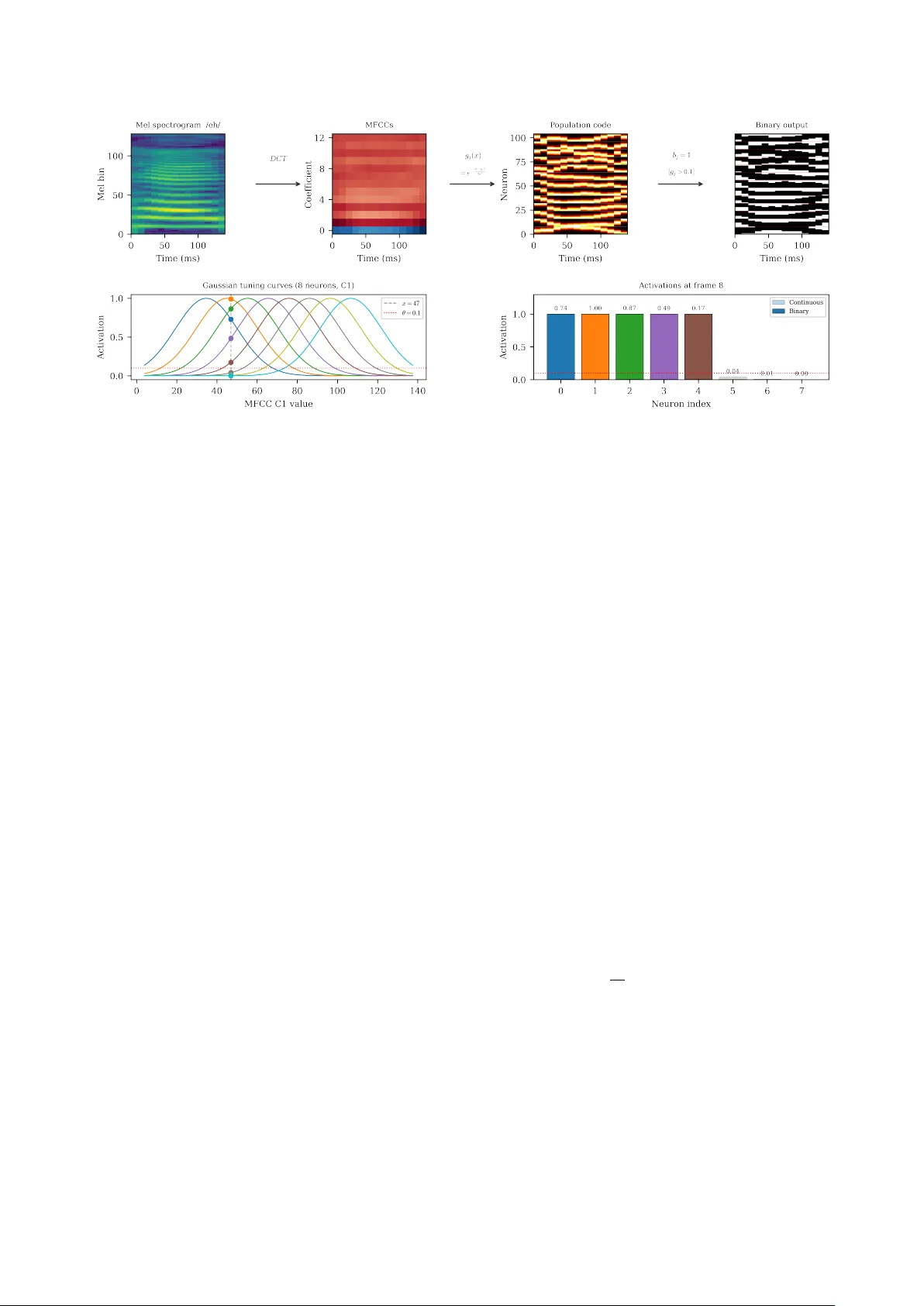
Loading high-quality paper...
Comments & Academic Discussion
Loading comments...
Leave a Comment