On Utility Maximization under Multivariate Fake Stationary Affine Volterra Models

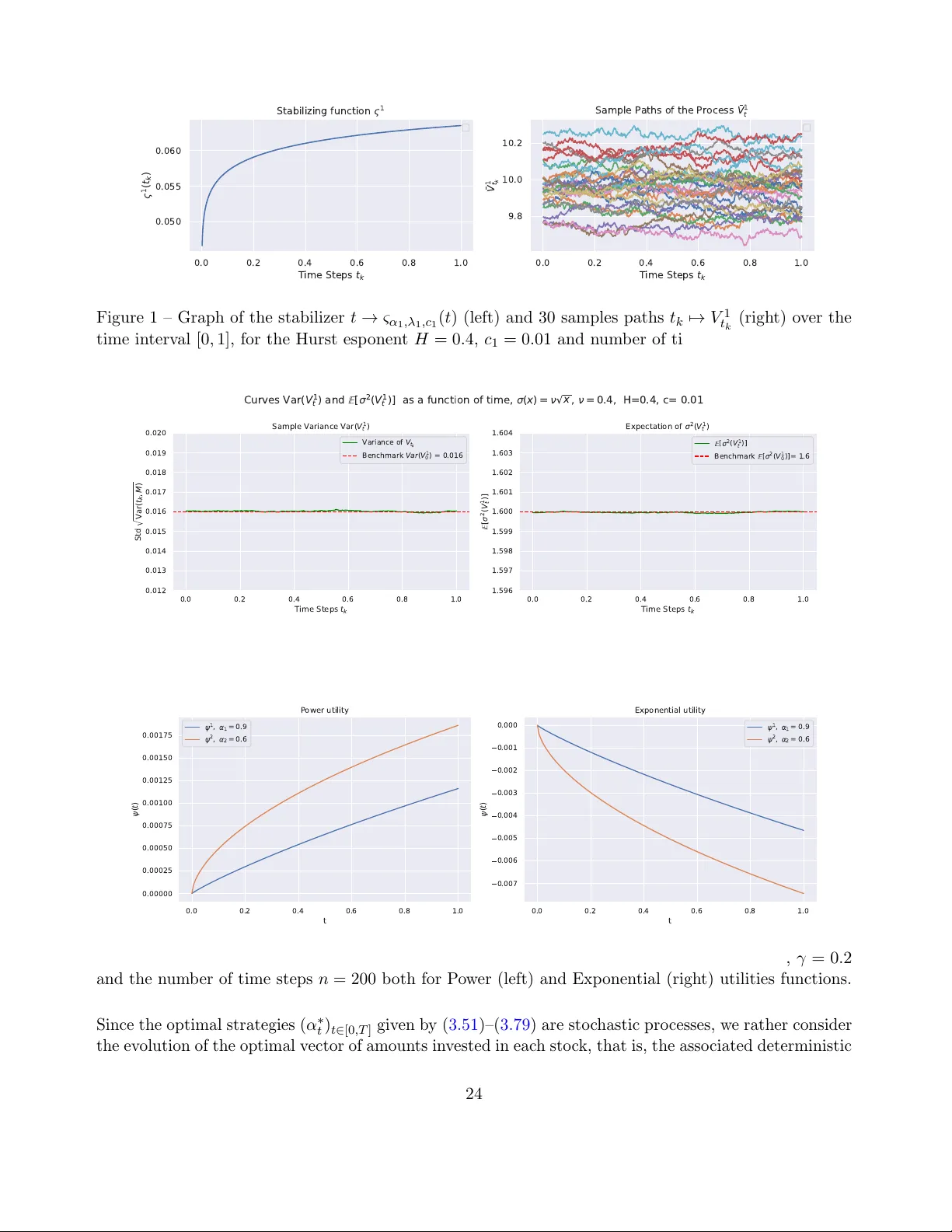
On Utilit y Maximization under Multiv ariate F ak e Stationary Aﬃne V olterra Mo dels Emman uel Gnab ey eu ∗ † Marc h 12, 2026 Abstract This pap er is concerned with Merton’s p ortfolio optimization problem in a V olterra sto c hastic en vironmen t describ ed by a m ultiv ariate fake stationary V olterra–Heston mo del. Due to the non- Mark o vianity and non-semimartingality of the underlying processes, the classical sto chastic con trol approac h cannot b e directly applied in this setting. Instead, the problem is tackled using a stochastic factor solution to a Riccati bac kward sto c hastic diﬀerential equation (BSDE). Our approach is inspired by the martingale optimality principle com bined with a suitable veriﬁcation argumen t. The resulting optimal strategies for Merton’s problems are derived in semi-closed form dep ending on the solutions to time-dep endent multiv ariate Riccati-V olterra equ ations. Numerical results on a tw o dimensional fake stationary rough Heston mo del illustrate the impact of stationary rough volatilities on the optimal Merton strategies. Keyw ords: Aﬃne V olterra Pro cesses, Sto c hastic Con trol, Martingale Optimality Principle, Back- w ard Sto c hastic Diﬀeren tial Equations (BSDE), F ractional Diﬀerential Equations, Riccati Equations, F unctional In tegral Equation. Mathematics Sub ject Classiﬁcation (2020): 34A08, 34A34, 45D05, 60G10, 60G22, 60H10, 91B70, 91G80,93E20 1 In tro duction The mo deling of asset price dynamics has undergone a paradigm shift with the empirical observ ation that b oth implied and realized volatilities of ma jor ﬁnancial indices exhibit signiﬁcantly rougher sample paths ( Gatheral et al. , 2018 ) than those generated by classical Bro wnian-motion-based mo dels. This observ ation has sparked a rapidly expanding b o dy of research on rough volatilit y mo dels. Motiv ated b y the widespread practical success of the celebrated Heston ( 1993 ) sto chastic volatilit y framew ork, sev eral rough extensions hav e b een prop osed, most notably the rough Heston model ( El Euc h and Rosen baum , 2019 ) builds on mark et microstructure and its generalisation, the V olterra Heston mo del in Abi Jab er et al. ( 2019 ). Recen t remark able adv ances include the in tro duction of the so-called fake stationary V olterr a Heston mo dels in Gnab eyeu et al. ( a , b ) with the aim of pro viding a uniﬁed and consisten t framework that captures b oth short- and long-maturity b eha viors and enables robust ﬁtting across the entire term structure. This broader class of volatilit y mo dels, encompassing the aforemen tioned sp eciﬁcations, is obtained by mo deling the v olatilit y pro cess as a sto chastic V olterra equation of con volution t yp e with a time-dep endent diﬀusion co eﬃcient. Therefore, this pap er fo cuses on the ﬁnancial mark et within the fak e stationary aﬃne V olterra mo del. ∗ Lab oratoire de Probabilit ´ es, Statistique et Mod´ elisation, UMR 8001, Sorbonne Universit ´ e and Universit ´ e Paris Cit´ e, 4 pl. Jussieu, F-75252 Paris Cedex 5, F rance. E-mail: emmanuel.gnabeyeu mbiada@sorbonne-universite.fr † This research beneﬁted from the support of ”Ecole Doctorale Sciences Mathematiques de Paris Cen tre”. 1 Substan tial progress has recently b een achiev ed in the study of option pricing problems and asymptotic analysis under rough v olatility dynamics. By contrast, p ortfolio optimization in such mo dels remains comparativ ely underexplored, although it has attracted gro wing in terest in recen t years. Notable con tributions include F ouque and Hu ( 2019 ); B¨ auerle and Desmettre ( 2020 ); Han and W ong ( 2020 ), whic h in v estigate optimal inv estment problems with p ow er utility in fractional Heston-t yp e mo dels. Despite these adv ances, the o verwhelming ma jority of dev elopmen ts in rough v olatility , whether for asset mo deling, deriv ative pricing, or p ortfolio selection, hav e b een conﬁned to the mono-asset case. F rom a practical standp oint, ho w e v er, m ulti-asset allo cation with correlated sources of risk constitutes a fundamental dimension of p ortfolio management; see, for instance, Burasc hi et al. ( 2010 ). Merton’s p ortfolio optimization problem which consists in maximizing an in v estor’s exp ected utility from terminal wealth with resp ect to a given utilit y function has served as a cornerstone in mathematical ﬁnance. It is the most classic ﬁnancial economic approac h to understand how the mark et volatilit y aﬀect inv estment demands. In the classical Heston ( 1993 ) sto chastic volatilit y framew ork, this problem w as solv ed explicitly in Kraft ( 2005 ), building on the represen tation results of Zariphop oulou ( 2001 ), and extensions to general aﬃne sto chastic v olatility mo dels w ere obtained in Kallsen and Muhle-Karb e ( 2010 ) using sto chastic control theory . In the V olterra framework, ho w ever, the volatilit y pro cess is non-Mark ovian, which preven ts the direct application of the classical sto chastic control metho ds based on the Hamilton–Jacobi–Bellman (HJB) partial diﬀeren tial equation. In order to circumv ent this diﬃcult y , Han and W ong ( 2020 ), inspired by F ouque and Hu ( 2019 ), adopt a martingale distortion ansatz and apply the martingale optimality principle to derive explicit optimal in vestmen t strategies in a single-asset or mono-asset V olterra–Heston mo del. Motiv ated by sev eral imp ortant empirical st ylized facts ab out real ﬁnancial markets suc h as c hoice among m ultiple assets, rough volatilit y b ehavior, correlations across sto cks or assets and leverage eﬀects (i.e., correlation b etw een a sto ck and its v olatility), m ultiv ariate rough v olatilit y mo dels hav e recently b een developed ; see, e.g., Abi Jab er et al. ( 2019 ); T omas and Rosen baum ( 2021 ). In Aichinger and Desmettre ( 2021 ), the authors analyze the Merton p ortfolio problems with pow er utilit y for a class of m ultiv ariate V olterra Heston mo dels that features b oth inter-asset correlations and correlation betw een a sto ck and its volatilit y . In the present pap er, we solve the Merton p ortfolio problem for in vestors with p o w er and exp onential utility functions, within the class of the so-called fake stationary multivariate aﬃne V olterr a mo dels . Main contributions. Building up on recent developmen ts in volatilit y and V olterra mo dels ( Gnab eyeu et al. , 2024 , a , b ) and motiv ate d by recent works and adv ances on multiv ariate V olterra volatilit y mo deling Abi Jab er et al. ( 2019 ); T omas and Rosenbaum ( 2021 ); Aichinger and Desmettre ( 2021 ), the primary ob jectiv e of this pap er is to adv ance the literature on utilit y maximization along t wo main directions: (i) W e in tro duce a class of multivariate fake stationary aﬃne V olterr a sto chastic volatility mo dels that capture k ey stylized features of ﬁnancial markets, including heterogeneous roughness across assets, p ossibly sto c hastic inter-asset correlations, and leverage eﬀects namely , dependence b et w een asset returns and their resp ective volatilities while main taining a consisten t mo deling framew ork across time scales, from short to long maturities. (ii) This mo del preserve analytical tractabilit y , thereby enabling explicit c haracterization of the optimal inv estmen t strategy for the Merton’s problem, despite the in trinsic c hallenges p osed b y m ultiv ariate non-Mark ovian dynamics. Organization of the W ork. The outline of the pap er is as follo ws: Section 2 giv es an ov erview of the mo del which is needed throughout the pap er: W e in tro duce the m ulti asset ﬁnancial market, where v olatility is mo deled by a multiv ariate class of fake stationary V olterr a squar e r o ot pr o c ess , and w e state 2 the optimization problem. F or suc h a mark et mo del we consider in section 3 tw o diﬀerent approaches to solve the Merton p ortfolio problem. More precisely , in section 3 we inv estigate the classical problem of maximizing the exp ected utility of terminal w ealth in a m ulti-asset fak e stationary V olterra–Heston v olatility market, for b oth p ow er and exp onen tial utility preferences. W e ﬁrst adapt the martingale distortion transformation used in F ouque and Hu ( 2019 ); Han and W ong ( 2020 ) to the (degenerate) m ultiv ariate case. How ever, as it is pointed out in Abi Jab er et al. ( 2021 ); Aichinger and Desmettre ( 2021 ), this only works if the correlation structure is highly degenerate. Inspired by the techniques used in B¨ auerle and Li ( 2013 ); Aichinger and Desmettre ( 2021 ), we then pro vide a solution for the Merton p ortfolio optimization problem for a more general correlation structure using a veriﬁcation argument. In Section 4 , we demonstrate the practical implications of our ﬁndings through n umerical exp eriments based on a tw o-dimensional fake stationary rough Heston mo del. Finally , Section 5 is devoted to the pro ofs of the main results. Notations. • Denote T = [0 , T ] ⊂ R + , Leb d the Leb esgue measure on ( R d , B or ( R d )), H := R d , etc. • X := C ([0 , T ] , H )( resp. C 0 ([0 , T ] , H )) denotes the set of con tinuous functions(resp. null at 0) from [0 , T ] to H and B or ( C d ) denotes the Borel σ -ﬁeld of C d induces by the sup-norm top ology . • F or p ∈ (0 , + ∞ ), L p H ( P ) or simply L p ( P ) denote the set of H -v alued random vectors X deﬁned on a probabilit y space (Ω , A , P ) suc h that ∥ X ∥ p := ( E [ ∥ X ∥ p H ]) 1 /p < + ∞ . • Let M denote the space of all ( R + , B or ( R ))-measurable functions m on R + suc h that the restriction µ | [0 ,T ] , for any T > 0, is a R -v alued ﬁnite measure (i.e. the restriction m | [0 ,T ] with T > 0 is w ell-deﬁned). F or m ∈ M and a compact set E ⊂ R + , we deﬁne the total v ariation of m on E b y: | m | ( E ) := sup n P N j =1 | m ( E j ) | : { E j } N j =1 is a ﬁnite measurable partition of E o . W e assume that the set of measure m ∈ M on R + is of lo cally b ounded v ariation. • Con volution betw een a function and a measure. Let f : (0 , T ] → R b e a measurable function and m ∈ M . Their conv olution (whenever the in tegral is well-deﬁned) is deﬁned by ( f ∗ m )( t ) = Z [0 ,t ) f ( t − s ) dm ( s ) = Z [0 ,t ) f ( t − s ) m ( ds ) = ( f m ∗ 1 ) t , t ∈ (0 , T ] . (1.1) • X ⊥ ⊥ Y stands for indep endence of random v ariables, v ectors or pro cesses X and Y . • F or a measurable function φ : R + → R , ∀ p ≥ 1 , we denote: ∥ φ ∥ p L p ([0 ,T ]) := R T 0 | φ ( u ) | p du, ∥ φ ∥ ∞ = ∥ φ ∥ sup := sup u ∈ R + | φ ( u ) | and ∥ φ ∥ ∞ ,T = ∥ φ ∥ sup ,T := sup u ∈ [0 ,T ] | φ ( u ) | . • Γ( a ) = R + ∞ 0 u a − 1 e − u du, a > 0 , and B ( a, b ) = R 1 0 u a − 1 (1 − u ) b − 1 du, a, b > 0 . W e set R + = [0 , + ∞ ), R − = ( −∞ , 0]. • Let [0 , T ] b e a ﬁnite time horizon, where T < ∞ . Giv en a complete probability space (Ω , F , P ) and a ﬁltration F = ( F t ) t ≥ 0 satisfying the usual conditions (W e equip (Ω , F , P ) with a righ t-con tinuous, P − complete ﬁltration F ), w e denote by L ∞ F ([0 , T ] , R d ) = n Y : Ω × [0 , T ] 7→ R d , F − prog. measurable and b ounded a.s. o L p F ([0 , T ] , R d ) =  Y : Ω × [0 , T ] 7→ R d , F − prog. measurable s.t. E h Z T 0 | Y s | p ds i < ∞  S ∞ F ([0 , T ] , R d ) = ( Y : Ω × [0 , T ] 7→ R d , F − prog. measurable s.t. sup t ≤ T | Y t ( w ) | < ∞ a.s. ) S p F ([0 , T ] , R d ) = ( Y : Ω × [0 , T ] 7→ R d , F − prog. measurable s.t. E h sup 0 ≤ t ≤ T | Y t | p i < ∞ ) . 3 Here | · | denotes the Euclidian norm on R d . Classically , for p ∈ (1 , ∞ ), we deﬁne L p,loc F ([0 , T ] , R d ) as the set of progressive pro cesses Y for which there exists a sequence of increasing stopping times τ n ↑ ∞ suc h that the stopp ed pro cesses Y τ n are in L p F ([0 , T ] , R d ) for ev ery n ≥ 1, and w e recall that it consists of all progressiv e pro cesses Y s.t. R T 0 | Y t | p dt < ∞ , a.s. Likewise for S p,loc F ([0 , T ] , R d ). T o unclutter notation, w e write L p,loc F ([0 , T ]) instead of L p,loc F ([0 , T ] , R d ) when the con text is clear. • W e will use the matrix norm | A | = tr( A ⊤ A ) in this pap er. Our problem is deﬁned under a giv en complete probabilit y space (Ω , F , P ), with a ﬁltration F = { F t } 0 ≤ t ≤ T satisfying the usual conditions, supp orting a 2 d -dimensional Brownian motion ( B , B ⊤ ) for d ≥ 1. The ﬁltration F is not necessarily the augmented ﬁltration generated b y ( B , B ⊤ ) ; th us, it can b e a strictly larger ﬁltration. Here P is a real-world probabilit y measure from whic h a family of equiv alent probability measures can b e generated. 2 Preliminaries: Multiv ariate fak e stationary aﬃne V olterra mo dels Fix T > 0, d ∈ N . W e let K = diag ( K 1 , . . . , K d ) b e diagonal with scalar k ernels K i ∈ L 2 ([0 , T ] , R ) on the diagonal, φ = diag ( φ 1 , . . . , φ d ), ν = diag ( ν 1 , . . . , ν d ), ς = diag ( ς 1 , . . . , ς d ) with ς i a (lo cally) b ounded Borel function and D := − diag ( λ 1 , . . . , λ d ) ∈ R d × d . Let V = ( V 1 , . . . , V d ) ⊤ b e the follo wing R d + –v alued scaled V olterra square–ro ot pro cess driven by an d -dimensional pro cess W = ( W 1 , . . . , W d ) ⊤ : V t = φ ( t ) V 0 + Z t 0 K ( t − s )  µ ( s ) + D V s  ds + Z t 0 K ( t − s ) ν ς ( s ) p diag( V s ) dW s , V 0 ⊥ ⊥ W . (2.2) Here µ : R + → R d , W is a d -dimensional Wiener pro cess. Note that the drift b ( t, x ) = µ ( t ) + D x is clearly Lipschitz contin uous in x ∈ R d , uniformly in t ∈ T + and b oth the drift term b and the diﬀusion co eﬃcien t σ ( t, x ) = ν ς ( t ) p diag( x ) are of linear gro wth, i.e. there is a constant C b,σ > 0 such that ∥ b ( t, x ) ∥ + ∥| σ ( t, x ) |∥ ≤ C b,σ (1 + ∥ x ∥ ) , for all t ∈ [0 , T ] and x ∈ R . W e alw ays work under the assumption b elo w, which applies to the inhomogeneous V olterra equation ( 2.2 ) . Assumption 2.1 (On V olterra Equations with conv olutiv e k ernels) . Assume that K is diagonal with sc alar kernels K i on the diagonal for i = 1 , . . . , d that is c ompletely monotone on (0 , ∞ ) and satisfy for any T > 0 , (i) Assume that the kernel K i is strictly p ositive and satisfy: — The inte gr ability assumption: The fol lowing is satisﬁe d for some b θ i ∈ (0 , 1] . ( b K cont b θ ) ∃ b κ i < + ∞ , ∀ ¯ δ ∈ (0 , T ] , b η ( δ ) := sup t ∈ [0 ,T ] " Z t ( t − ¯ δ ) + K i  t − u  2 du # 1 2 ≤ b κ i ¯ δ b θ i . (2.3) — The c ontinuity assumption: ( K cont θ ) ∃ κ i < + ∞ , ∃ θ i ∈ (0 , 1] such that ∀ ¯ δ ∈ (0 , T ) ( K cont θ ) ∀ ¯ δ ∈ (0 , T ) , η ( ¯ δ ) := sup t ∈ [0 ,T ]  Z t 0 | K i (  s + δ ) ∧ T  − K i ( s ) | 2 ds  1 2 ≤ κ i ¯ δ θ i . (2.4) (ii) Final ly, assume that V i 0 ∈ L p ( P ) for some suitable p ∈ (0 , + ∞ ) , such that the pr o c ess t → v i 0 ( t ) = V 0 φ i ( t ) is absolutely c ontinuous and ( F t ) -adapte d. Mor e over, for some δ i > 0 , for any p > 0 , E  sup t ∈ [0 ,T ] | v i 0 ( t ) | p  < + ∞ , E  | v i 0 ( t ′ ) − v i 0 ( t ) | p  ≤ C T ,p  1 + E  sup t ∈ [0 ,T ] | v i 0 ( t ) | p   | t ′ − t | δ i p . 4 Remark: F or i = 1 , . . . , d , as K i is completely monotone on (0 , ∞ ) and not iden tically zero, we hav e that K i is nonnegative, not identically zero, non-increasing and con tinuous on (0 , ∞ ), and it follows from ( B. Grip enberg and Saa v alainen , 1990 , Theorem 5.5.4) that K i has a resolven t of the ﬁrst kind r i whic h is nonnegative and non-increasing in the sense that s 7→ r i ([ s, s + t ]) is non-increasing for all t ≥ 0. In the case of α − fractional kernel (corresp onding to K i = K α i with α i ∈ [ 1 2 , 1)), b y Gnab ey eu et al. ( b ) Equation ( 2.2 ) admits at least a unique-in-la w p ositiv e w eak solution as a scaling limit of a sequence of time-mo dulated Hawk es pro cesses with heavy-tailed kernels in a nearly unstable regime. Moreov er, under assumption 2.1 for some p > 0, a solution t 7→ V t to Equation ( 2.2 ) starting from V 0 has a  δ ∧ ϑ ∧ β − 1 2 β − η  -H¨ older path wise con tinuous mo diﬁcation on R d + for suﬃciently small η > 0 and satisfying (among other prop erties), ∀ T > 0 , ∃ C T ,p > 0 ,   sup t ∈ [0 ,T ] ∥ V t ∥   p ≤ C T ,p 1 +   sup t ∈ [0 ,T ] ∥ φ ( t ) V 0 ∥   p ! . (2.5) Note that under our assumptions, if p > 0 and E [ ∥ φ ( t ) V 0 ∥ p ] < + ∞ for every t ≥ 0, then by ( 2.5 ) , E [ sup t ∈ [0 ,T ] ∥ V t ∥ p ] < C T (1 + E [ sup t ∈ [0 ,T ] ∥ φ ( t ) V 0 ∥ p ]) < + ∞ for every T > 0. Combined with the linear gro wth in Assumption 2.1 (ii) ∥| σ ( t, x ) |∥ ≤ C ′ T (1+ ∥ x ∥ ) for t ∈ [0 , T ], this implies E [ sup t ∈ [0 ,T ] ∥| σ ( t, X t ) |∥ p ] < C ′ T (1 + E [ sup t ∈ [0 ,T ] ∥ φ ( t ) V 0 ∥ p ]) < + ∞ for every T > 0, enabling the unrestricted use of b oth regular and sto c hastic F ubini’s theorems. Suﬃcient conditions for interc hanging the order of ordinary integration (with resp ect to a ﬁnite measure) and sto chastic integration (with resp ect to a square in tegrable martingale) are pro vided in ( Kailath et al. , 1978 , Thm.1), and further details can b e found in ( Protter , 2005 , Thm. IV.65), ( W alsh , 1986 , Theorem 2.6), ( V eraar , 2012 , Theorem 2.6). Remark 2.1. This c overs, for instanc e, c onstant non-ne gative kernels, fr actional kernels of the form t α − 1 Γ( α ) 1 R + with α ∈ ( 1 2 , 1] , exp onential ly de c aying kernels e − β t with β > 0 and mor e gener al ly the gamma kernel K ( t ) = t α − 1 Γ( α ) e − β t 1 R + with α ∈  1 2 , 1  and β ≥ 0 ( se e e.g. ( Gnab eyeu and Pag` es , 2025 , Pr op ositions 6.1 and 6.3)). The r oughness of the volatility p aths is determine d by the p ar ameter α linke d to the Hurst p ar ameter H via the r elation α = H + 1 2 . F or α → 1 we r e c over the classic al markovian squar e r o ot pr o c ess. 2.1 Stabilizer and fak e stationarity regimes. Deﬁnition 2.2 (F ake Stationarity Regimes) . L et ( V t ) t ≥ 0 b e a solution to the sc ale d V olterr a e qua- tion ( 2.2 ) starting fr om any V 0 ∈ L 2 ( P ) . Then, the pr o c ess ( V t ) t ≥ 0 exhibit a fake stationary r e gime of typ e I in the sense of Pag` es ( 2024 ); Gnab eyeu and Pag` es ( 2025 ) if it has c onstant me an and varianc e over time i.e.: ∀ t ≥ 0 , E [ V t ] = c ste and V ar ( V t ) = c ste = v 0 ∈ R d + . (2.6) F or ev ery λ ∈ R , the r esolvent or Solvent c or e R λ asso ciated to a real-v alued k ernel K , known as the λ -r esolvent of K is deﬁned as the unique solution – if it exists – to the deterministic V olterra equation ∀ t ≥ 0 , R λ ( t ) + λ Z t 0 K ( t − s ) R λ ( s ) ds = 1 . (2.7) or, equiv alen tly , written in terms of conv olution, R λ + λK ∗ R λ = 1 and admits the formal Neumann series exp ansion R λ = 1 ∗  P k ≥ 0 ( − 1) k λ k K k ∗  where K k ∗ denotes the k -th conv olution of K with the con ven tion, K 0 ∗ = δ 0 (Dirac mass at 0). 5 Remark If K is regular enough (say con tinuous) the resolven t R λ is diﬀerentiable and one c hecks that f λ = − R ′ λ satisﬁes for ev ery t > 0, − f λ ( t ) + λ  R λ (0) K ( t ) − K ∗ f λ ( t )  = 0 that is f λ is solution to the equation f λ + λK ∗ f λ = λK and reads f λ = X k ≥ 1 ( − 1) k λ k K k ∗ , K 0 ∗ = δ 0 . (2.8) Example 2.3. Denote by E α the standar d Mittag-L eﬄer function. F or the α − fr actional kernels deﬁne d in R emark 2.1 the identity K α ∗ K α ′ = K α + α ′ holds for t ≥ 0 so that R α,λ ( t ) = X k ≥ 0 ( − 1) k λ k t αk Γ( αk + 1) = E α ( − λt α ) , and f α,λ ( t ) = − R ′ α,λ ( t ) = λt α − 1 X k ≥ 0 ( − 1) k λ k t αk Γ( α ( k + 1)) . W e will alwa ys work under the following assumption. Assumption 2.2 ( λ -resolv ent R λ of the k ernel) . F or i = 1 , · · · , d , we assume that the λ i -r esolvent R λ i of the kernel K i satisﬁes the fol lowing for every λ i > 0 : ( K )        ( i ) R λ i ( t ) is diﬀer entiable on R + , R λ i (0) = 1 and lim t → + ∞ R λ i ( t ) = a i ∈ [0 , 1[ , ( ii ) f λ i ∈ L 2 lo c ( R + , L eb 1 ) , for t > 0 , L f λ i ( t )  = 0 dt − a.e., wher e f λ i := − R ′ λ i , ( iii ) φ i ∈ L 1 R + ( L eb 1 ) , is a c ontinuous function satisfying lim t →∞ φ i ( t ) = φ i ∞ , with a i φ i ∞ < 1 , ( iv ) µ is a C 1 -function such that ∥ µ ∥ sup < ∞ and lim t → + ∞ µ ( t ) = µ ∞ ∈ R d . (2.9) Remark: Under the assumption ( K ), f λ i is a (1 − a i )-sum measure, i.e., R + ∞ 0 f λ i ( s ) ds = 1 − a i . F urthermore, lim t → + ∞ R t 0 f λ i ( t − s ) µ i ( s ) ds = µ i ∞ and lim t → + ∞ φ i ( t ) − ( f λ i ∗ φ i )( t ) = φ i ∞ a i . (see ( Gnab ey eu and Pag ` es , 2025 , Lemma 3.1)). Finally , if f λ i = − R ′ λ i > 0 for t > 0, then f λ i is a probability densit y in which case, R λ i is non-increasing. This is in particular the case for the Mittag-Leﬄer densit y function f α i ,λ i for α i ∈ ( 1 2 , 1), in which case f α i ,λ i is a completely monotonic function (hence conv ex), decreasing to 0 while 1 − R α i ,λ i is a Bernstein function (see e.g. ( Gnab ey eu and Pag ` es , 2025 , Prop osition 6.1)). The Prop osition b elow shows what are the c onsequences of the three constraints in equation ( 2.6 ) . Prop osition 2.4 (F ake stationary V olterra square ro ot pro cess.) . L et ( V t ) t ≥ 0 b e a solution to the sc ale d V olterr a squar e r o ot e quation in its form ( 2.2 ) starting fr om any r andom variable V 0 ∈ L 2 (Ω , F , P ) . Then, a ne c essary and suﬃcient c ondition for the r elations ( 2.6 ) to b e satisﬁe d is that for i = 1 , . . . , d E [ V i 0 ] = 1 − a i 1 − a i φ i ∞ µ i ∞ λ i := x i ∞ and ∀ t ≥ 0 , φ i ( t ) = 1 − λ i Z t 0 K i ( t − s )  µ i ( s ) λ i x i ∞ − 1  d s. (2.10) so that ( 2.2 ) r e ads: V i t = V i 0 − 1 λ i x i ∞  V i 0 − x i ∞  Z t 0 f λ i ( t − s ) µ i ( s ) d s + 1 λ i Z t 0 f λ i ( t − s ) ς i ( s ) p V i s dW i s . (2.11) and the c ouple ( v i 0 , ς i ( t )) , wher e v i 0 = V ar ( V i 0 ) must satisfy the functional e quation: ( E λ i ,c i ) : ∀ t ≥ 0 , c i λ 2 i  1 − ( φ i ( t ) − ( f λ i ∗ φ i ) t ) 2  = ( f 2 λ i ∗ ς i 2 )( t ) wher e c i = v i 0 ν 2 i x i ∞ i.e. ς i = ς i λ i ,c i . (2.12) Pro of : This is a straightforw ard extension to the multi-dimensional setting of ( Gnab eyeu and P ag` es , 2025 , Prop osition 3.4 and Theorem 3.5) (see also ( Gnab ey eu et al. , a , Prop osition 4.2 and 4.4)). Deﬁnition 2.5. We wil l c al l the stabilizer (or c orr e ctor) of the sc ale d sto chastic V olterr a e quation ( 2.2 ) the (lo c al ly) b ounde d Bor el function ς = diag ( ς 1 , . . . , ς d ) wher e ς i is a solution(if any) to the functional e quation ( E λ i ,c i ) in ( 2.12 ) for i = 1 , . . . , d . 6 Example 2. 6. Within the setting φ i ( t ) = φ i (0) = 1 for al l t ≥ 0 and K i the α − fr actional kernel deﬁne d in R emark 2.1 and Example 2.3 with α i ∈  1 2 , 1  , we have lim t → + ∞ R α i ,λ i = 0 . Setting a k = 1 Γ( αk +1) , b k = 1 Γ( α ( k +1)) , k ≥ 0 , then the stabilizer ς = ς α i ,λ i ,c i exists as a non-ne gative, non- incr e asing c onc ave function, on (0 , + ∞ ) (se e ( Pag` es , 2024 , Se ctions 5.1 and 5.2 ), ( Gnab eyeu and Pag ` es , 2025 , Se ctions 5.1 and 5.2 )), such that: ς 2 α i ,λ i ,c i ( t ) = c i λ 2 − 1 α i i ς 2 α i ( λ 1 α i i t ) wher e ς 2 α i ( t ) := 2 t 1 − α i P k ≥ 0 ( − 1) k c k t α i k and the c o eﬃcients ( c k ) k ≥ 0 ar e deﬁne d by the r e curr enc e formula c 0 = Γ( α ) 2 Γ(2 α − 1)Γ(2 − α ) and for every k ≥ 1 c k = Γ( α ) 2 Γ( α ( k + 1)) Γ(2 α − 1)Γ( αk + 2 − α ) " ( a ∗ b ) k − α ( k + 1) k X ℓ =1 B  α ( ℓ + 2) − 1 , α ( k − ℓ − 1) + 2  ( b ∗ 2 ) ℓ c k − ℓ # . (2.13) wher e for two se quenc es of r e al numb ers ( u k ) k ≥ 0 and ( v k ) k ≥ 0 , the Cauchy pr o duct is deﬁne d as ( u ∗ v ) k = P k ℓ =0 u ℓ v k − ℓ and B ( a, b ) = R 1 0 u a − 1 (1 − u ) b − 1 du denoting the b eta function. Mor e over,  lim inf k  | c k | 1 /k  − 1 /α = ∞ , ς α i ,λ i ,c i (0) = 0 and lim t → + ∞ ς α i ,λ i ,c i ( t ) = √ c i λ i ∥ f α i ,λ i ∥ L 2 ( L eb 1 ) . Set E D,c = S d i =1 E λ i ,c i . F rom no w on, w e will assume that there exists a unique p ositive b ounded Borel solution ς = ς D,c on (0 , + ∞ ) of the system of equation ( E D,c ) so that, the corresp onding time- inhomogeneous V olterra square ro ot equation ( 2.2 ) is refered to as a Multivariate Stabilize d V olterr a Cox-Ingersol l-R oss (CIR) e quation or as a Multivariate fake stationary V olterr a CIR e quation if, in addition, equation ( 2.10 ) holds. 2.2 F orm ulation of the sto chastic Market mo del W e consider a ﬁnancial mark et on [0 , T ] on some ﬁltered probability space (Ω , F , F := ( F t ) t ≥ 0 , P ) with d + 1 securities, consisting of a b ond and d sto c ks. The non–risky asset S 0 satisﬁes the (sto c hastic) ordinary diﬀerential equation: dS 0 t = S 0 t r ( t ) dt, with a time-dep enden t deterministic short risk-free rate r : R + → R , and d risky assets (sto c k or index) whose return v ector pro cess ( S t ) t ≥ 0 = ( S 1 t , . . . , S d t ) t ≥ 0 is deﬁned via the dynamics given b y the v ector-sto c hastic diﬀeren tial equation (SDE): dS t = diag( S t )  r ( t ) 1 d + σ t λ t  dt + σ t dB t  , (2.14) driv en by a d -dimensional Brownian motion B , with a d × d -matrix v alued contin uous sto chastic v olatility pro cess σ whose dynamics is driven b y ( 2.2 ) and a R d -v alued con tin uous sto chastic pro cess λ , called market pric e of risk . Here 1 d denotes the vector in R d with all comp onents equal to 1 and the correlation structure of W with B is given by W i = ρ i B i + q 1 − ρ 2 i B ⊥ ,i = Σ ⊤ i B t + q 1 − Σ ⊤ i Σ i B ⊥ ,i t , i = 1 , . . . , d, (2.15) for some ( ρ 1 , . . . , ρ d ) ∈ [ − 1 , 1] d , where (0 , . . . , ρ i , . . . , 0) ⊤ := Σ i ∈ R d is such that Σ ⊤ i Σ i ≤ 1, and B ⊥ = ( B ⊥ , 1 , . . . , B ⊥ ,d ) ⊤ is an d –dimensional Brownian motion indep endent of B . The correlation ρ i b et w een sto c k price S i and v ariance V i is assumed constan t. Note that d ⟨ W i ⟩ t = dt but W i and W j can b e correlated, hence W is not necessarily a Brownian motion. Observ e that pro cesses λ and σ are F -adapted, p ossibly unbounded, but not necessarily adapted to the ﬁltration generated by W . W e p oin t out that F ma y b e strictly larger than the augmen ted ﬁltration generated by B and B ⊥ as we deal with weak solutions to sto chastic V olterra equations. 7 W e assume that σ in ( 2.14 ) is given by σ = p diag( V ) , where the R d + –v alued scaled pro cess V is deﬁned in ( 2.2 ) with ς = ς D,c and Equation ( 2.10 ) holds true. W e will b e chieﬂy interested in the case where λ t is linear in σ t . More sp eciﬁcally , the the market price of risk (risk premium) is assumed to be in the form λ =  θ 1 √ V 1 , . . . , θ d √ V d  ⊤ , for some constan t θ i ≥ 0, so that the dynamics for the stock prices ( 2.14 ) reads following Kraft ( 2005 ); Abi Jab er et al. ( 2019 ) dS i t = S i t  r ( t ) + θ i V i t  dt + S i t q V i t dB i t , i = 1 , . . . , d. (2.16) Since S is fully determined by V , the existence of S readily follows from that of V . In particular, weak existence of H¨ older path wise con tinuous solution V of ( 2.2 ) suc h that ( 2.5 ) holds is established under suitable assumptions on the kernel K and sp eciﬁcations g 0 as shown in the following remark. W e state the following existence and uniqueness result from Gnab eyeu et al. ( b ) which is extended to the multi-dimensional setting. Theorem 2.7. (( Gnab eyeu et al. , b , The or em 3.1 and R emark on The or em 3.2)). Under Assumption 2.1 , the sto chastic V olterr a e quation ( 2.16 )-( 2.2 ) has a unique in law c ontinuous R d + × R d + -value d we ak solution ( S, V ) for any initial c ondition ( S 0 , V 0 ) ∈ R d + × R d + deﬁne d on some ﬁlter e d pr ob ability sp ac e (Ω , F , ( F ) t ≥ 0 , P ) such that sup t ≤ T E [ ∥ V t ∥ p ] < ∞ , p > 0 . (2.17) F rom no w on, w e set g 0 ( t ) := φ ( t ) V 0 + R t 0 K ( t − s ) µ ( s ) ds and d Z t = D V t dt + ν p diag( V t ) dW t , ∀ t ≥ 0 so that Equation ( 2.2 ) reads V t = g 0 ( t ) + Z t 0 K ( t − s ) D V s ds + Z t 0 K ( t − s ) ν ς ( s ) p diag( V s ) dW s = g 0 ( t ) + Z t 0 K ( t − s ) d Z s . (2.18) Finally , w e consider the R d -v alued pro cess for s ≥ t, g t ( s ) = g 0 ( s ) + Z t 0 K ( s − u )  D V u du + ν ς ( s ) p diag( V u ) dW u  = g 0 ( s ) + Z t 0 K ( s − u ) d Z u . (2.19) One notes that for each, s ≤ T , ( g t ( s )) t ≤ s is the adjusted forw ard pro cess g t ( s ) = E h V s − Z s t K ( s − u ) D V u du    F t i . (2.20) This adjusted forward pro cess is commonly used (see, e.g., Abi Jab er et al. ( 2021 )) to elucidate the aﬃne structure of aﬃne V olterra pro cesses with contin uous tra jectories. The pro cess in ( 2.18 ) is non-Marko vian and non-semimartingale in general. Note that our mo del ( 2.16 )- ( 2.15 )-( 2.2 ) features correlation b etw een the sto cks and b et ween a sto c k and its volatilit y . Moreov er, the metho dology dev elop ed in this pap er, and hence the results obtained, remain v alid if the matrix D in ( 2.2 ) is not assumed to b e diagonal, but only satisﬁes D ∈ R d × d , D ij ≥ 0 for i  = j. This also provides an extension to the inhomogeneous setting of the mo dels considered in Abi Jab er et al. ( 2019 , 2021 ); Aichinger and Desmettre ( 2021 ). 8 3 Merton’s p ortfolio problem: Utilit y maximisation  Preliminaries and Problem form ulation : As we deal with w eak solutions to sto chastic V olterra equations ( 2.16 )-( 2.2 ), Brownian motion is also a part of the solution. How ever, exp ected utility only dep ends on the exp ectation of the wealth pro cess. In the sequel, we ﬁx a version of the solution ( S, V , B , B ⊤ ) to ( 2.16 )-( 2.2 ) as other solutions ha v e the same law. W e consider the classical problem of maximizing the exp ected utility of terminal w ealth. A p ortfolio strategy α t = ( α t, 1 , . . . , α t,d ) ⊤ is an R d -v alued, F -progressiv ely measurable pro cess, where α t,k represen ts the prop ortion of w ealth inv ested in asset k at time t . Under a ﬁxed p ortfolio strategy , the corresp onding w ealth pro ces s ( X α t ) t ≥ 0 dep end on V in ( 2.2 ) and has a certain dynamic to b e sp eciﬁed latter. By A w e denote the set of admissible p ortfolio or inv estment strategies i.e. the set of all F -progressiv ely measurable pro cesses ( α t ) t ∈ [0 ,T ] v alued in the Polish space R d . T o ease notation burden, whenever the context is clear, we simply write X , instead of X α , as the wealth pro cess under α ∈ A with initial condition X 0 = x 0 > 0 and V 0 > 0. Deﬁnition 3.1. 1. A utility function is a strictly incr e asing and strictly c onc ave function U : (0 , ∞ ) → R ∪ {−∞} , which is c ontinuously diﬀer entiable on (0 , ∞ ) . In the fol lowing, U denotes a gener al utility function. L ater, we wil l fo cus on p ower utility functions of the form U ( x ) = x γ γ , for γ ∈ R + \ { 0 , 1 } , or alternatively on exp onential utility functions of the form U ( x ) = − 1 γ e − γ x , for γ > 0 . γ is typic al ly c al le d the risk aversion p ar ameter. 2. A n admissible str ate gy α ∈ A is said to b e optimal (for terminal we alth) if it maximizes α 7− → E  U ( X α T )  over al l admissible str ate gies in A . That is the p ortfolio str ate gy α ∗ for which the supr emum is attaine d The inv estor’s goal in the Merton problem is to ﬁnd an optimal strategy so as to maximize the exp ected utilit y of terminal wealth. Sp eciﬁcally , given the utilit y function U on (0 , ∞ ) and starting from an initial capital x 0 > 0, the ob jectiv e of the agen t is V ( x 0 , V 0 ) := sup α ( · ) ∈ A E [ U ( X α T )] , given x 0 and V 0 . (3.21) with X α the wealth controlled by α ∈ A , starting from x 0 at time 0 and A the subset of controls α ∈ A suc h that the family { U ( X α τ ) : τ ∈ [0 , T ] } is uniformly integrable. The preferences of the agent are thus describ ed by the utilit y function U . Mathematically , w e aim at identifying the optimal v alue asso ciate d with the utility maximization problem deﬁned o v er a ﬁnite horizon T by V t ( x, v ) := ess sup α ∈ A t E x,v h U  X t,x,v ,α T  | F t i , x > 0 , v > 0 , t ∈ [0 , T ] , (3.22) and the optimal strategy α ∗ , given the preference describ ed b y the utilit y function U ( · ). This is a standard sto chastic control problem. The set A t is the class of all admissible strategies from t with zero b eing an absorbing state for X α t (bankruptcy). Here E x,v denotes exp ectation under the conditional distribution giv en X t = x and V t = v , and where the supremum is tak en ov er all admissible p ortfolio strategies. The F -adapted pro cess { V t , 0 ≤ t ≤ T } is a sup ermartingale. Moreo v er, there exists an optimal control α ∗ ∈ A for ( 3.21 ) if and only if the martingale prop erty holds, that is, the pro cess { V ∗ t , 0 ≤ t ≤ T } for α ∗ is a martingale. The idea is that an admissible control (or startegy) is optimal 1 if the asso ciated 1. optimal strategy: No exp ected gain from deviation, this implies martingality 9 v alue pro cess is a martingale and for an y other admissible control, it is a sup ermartingale. That is the classic martingale optimality principle , see, e.g., Hu et al. ( 2005 ), Pham ( 2009 , Section 6.6.1) or Jean blanc et al. ( 2012 ). Deﬁnition 3.2 (Martingale optimality principle) . The Pr oblem ( 3.21 ) c an b e solve d by c onstructing a family of pr o c esses { J α t } t ∈ [0 ,T ] , α ∈ A , satisfying the c onditions: 1. J α T = U ( X T ) for al l α ∈ A ; 2. J α 0 is a c onstant, indep endent of α ∈ A ; 3. J α t is a sup ermartingale for al l α ∈ A , and ther e exists α ∗ ∈ A such that J α ∗ is a martingale. A family of pro cesses with the ab o ve prop erties can now b e used to compare the exp ected utilities of an arbitrary strategy α ∈ A and the strategy α ∗ : E [ U ( X α T )] = E [ J α T ] ≤ J α 0 = J α ∗ 0 = E [ J α ∗ T ] = E [ U ( X α ∗ T )] = V ( x 0 , V 0 ) . where X α ∗ is the wealth pro cess under α ∗ . Thus the strategy α ∗ is indeed our desired optimal p ortfolio strategy . As stated before, Problem ( 3.21 ) seen as an optimization problem with state pro cess X α is non-Marko vian and the standard sto chastic con trol approac h cannot b e applied. Heuristically sp eaking, the non- Mark ovian and non-semimartingale characteristics of the multiv ariate fake stationary V olterra Heston mo del ( 2.16 )-( 2.2 ) are ov ercome in the degenerate correlation case by applying the martingale optimality principle and constructing an ansatz, which is inspired by the martingale distortion transformation and the exp onential-aﬃne represen tation (see e.g. ( Gnab ey eu , 2026 , Theorem A.4.)) in term of an auxiliary pro cess denoted Γ ≡ Γ( V t ) (more precisely Γ( g t )). In the general correlation case, we pro vide a veriﬁcation argumen t av oiding restrictions on the correlation structure linked to the martingale distortion transformation. In fact, F ouque and Hu ( 2019 ) show ed that if the Sharp e-ratio λ in 2.14 is b ounded and has b ounded deriv ative, then the v alue pro cess V t can b e e xpressed as V t ( x, v ) = J t ( X α t = x, V t = v ), where J t ( X α t , V t ) := F ( t, X α t )Γ( V t ) (3.23) for the p ow er utility case ( F ( t, X α t ) = U ( X α t ) = ( X α t ) γ γ ) even if the v olatility pro cess V t is non-Marko vian. This approac h is called the martingale distortion transformation and w as ﬁrst introduced in the seminal pap er Zariphop oulou ( 2001 ) and later transferred to a non-Marko vian setting with H¨ older- t yp e inequalities in T ehranchi ( 2004 ) for b oth p o w er utility and exponential utility case (in which F ( t, X α t ) = − 1 γ exp  − γ e R T t r ( s ) ds X α t  ). The extension to the m ulti-asset case is straight forward in the case of a b ounded risk premium and degenerate correlation structure(cf. F ouque and Hu ( 2019 ), Remark 2.5.). W e will provide concrete sp eciﬁcations of the pro cess Γ dep ending on the problem at hand. The semi-closed form exp onential–aﬃne representation ( Gnab eyeu , 2026 , Theorem A.4.) of the functional Γ can b e expressed in terms of the con tinuous solution ψ of an asso ciated time-inhomogeneous Riccati-type V olterra equation, which can be solv ed by well-kno wn eﬃcient n umerical metho ds. Note that, in contrast to Han and W ong ( 2020 ); Aichinger and Desmettre ( 2021 ), this representation is expressed in terms of the adjusted forward pro cess, as deﬁned in ( 2.19 ) – ( 2.20 ) , rather than the forw ard pro cess used in these works. W e oﬀer explicit solutions to the optimal p ortfolio p olicies that dep end on the function ψ , solution of the ab o ve-men tionned time-dep enden t multiv ariate Riccati-V olterra equation. Let Λ b e deﬁned as Λ i t = ν i ς i ( t ) ψ i ( T − t ) q V i t , i = 1 , . . . , d, 0 ≤ t ≤ T , (3.24) 10 W e will work under the follo wing assumption, Assumption 3.1. Assume that ther e exists a solution ψ ∈ C ([0 , T ] , R d ) to the ab ove-mentione d inhomo gene ous Ric c ati–V olterr a e quation satisfying the b elow appr opriate b ounde dness c ondition i.e. such that max 1 ≤ i ≤ d sup t ∈ [0 ,T ]  θ 2 i + ν 2 i ς i ( t ) 2 ψ i ( T − t ) 2  ≤ a a ( p ) , (3.25) holds for a suﬃcient lar ge p > 1 , wher e the c onstant a ( p ) is given by a ( p ) = max h p (2 + | Σ | ) , 2(8 p 2 − 2 p )  1 + | Σ | 2  , p  1 + | Σ | 2  i . (3.26) and the c onstant a > 0 is such that E h exp  a R T 0 P d i =1 V i s ds  i < ∞ . Remark on Assumption 3.1 : Note that if Assumption 3.1 hold, then E h exp  a ( p ) Z T 0  | λ s | 2 + | Λ s | 2  ds i < ∞ , (3.27) holds for some p > 1 and a constant a ( p ) giv en by ( 3.26 ). In fact, under Assumption 3.1 , we will hav e a ( p )  | λ s | 2 + | Λ s | 2  = a ( p ) d X i =1 V i s  θ 2 i + ν 2 i ς i ( s ) 2 ψ i ( T − s ) 2  ≤ a d X i =1 V i s , (3.28) whic h implies that E h exp  a ( p ) R T 0  | λ s | 2 + | Λ s | 2  ds i < ∞ . Remark: Condition ( 3.25 ) concerns the risk premium constants ( θ 1 , . . . , θ d ). F or a large enough constan t a > 0, from ( Gnab eyeu , 2026 , Theorem A.4.) ( with M ∋ m ( d s ) := a 1 d δ 0 ( d s )), a suﬃcient condition ensuring E  exp  a R T 0 P d i =1 V i s ds  < ∞ is the existence of a contin uous solution ˜ ψ on [0 , T ] to the inhomogeneous Riccati–V olterra equation ˜ ψ i ( t ) = Z t 0 K i ( t − s )  a +  D ⊤ ˜ ψ ( s )  i + ν 2 i 2 ( ς i ( T − s ) ˜ ψ i ( s )) 2  ds, i = 1 , . . . , d, 0 ≤ t ≤ T . (3.29) P ow er and exp onen tial utility functions are widely adopted in the literature and displa y distinct risk- a version prop erties. Speciﬁcally , the p ow er utilit y function exhibits constan t relativ e risk av ersion (CRRA), whereas the exp onential utilit y function is characterized by c onstan t absolute risk av ersion (CARA). Optimal strategies corresponding to these utility functions are presented in the sequel, within the framework of the mo del introduced in Section 2 . 3.1 Optimal strategy for the p o wer utility maximization problem Here, we denote by π t the prop ortion of wealth inv ested in the risky assets S . An agent inv ests at an y time t the prop ortion π t of his wealth X π t in the sto cks S of price’s vector S t , and the remaining prop ortion 1 − π ⊤ t 1 d in a b ond of price S 0 t with in terest rate r ( t ). The notation X π t emphasizes the dep endence of the wealth on the strategy π = ( π t ) t ≥ 0 . The p ortfolio strategy π t = ( π 1 t , . . . , π d t ) is an ( R d ) ∗ v alued, progressiv ely measurable pro cess, where π k t represen ts the prop ortion of w ealth inv ested 11 in to sto ck k at time t . Assuming the mo del ( 2.14 ) – ( 2.16 ) for S t , the dynamics of the controlled wealth pro cess is giv en b y d X π t = X π t  π ⊤ t  r ( t ) 1 d + σ ( V t ) λ t  + (1 − π ⊤ t 1 d ) r ( t )  d t + X π t π ⊤ t σ ( V t ) d B t = X π t  r ( t ) + π ⊤ t σ ( V t ) λ t  d t + X π t π ⊤ t σ ( V t ) d B t = X π t ( r ( t ) + π ⊤ t diag( V t ) θ ) dt + X t π ⊤ t p diag( V t ) dB t , where θ = ( θ 1 , . . . , θ d ) ⊤ . The in vestor faces the p ortfolio constraint that, at an y time t , π t tak es v alues in a closed con vex subset A ⊂ R d denoting the set of admissible p ortfolio strategies. F rom now, we let α t := σ ( V t ) ⊤ π t b e the inv estmen t strategy . Then, under a ﬁxed p ortfolio strategy , the w ealth pro cess X α t , controlled by α is gov erned by: dX α t =  r ( t ) + α ⊤ t λ t  X α t dt + α ⊤ t X α t dB t , X 0 = x 0 > 0 . (3.30) By solving the linear SDE ( 3.30 ), the wealth pro cess admits the explicit represen tation X α t = x 0 exp  Z t 0  r ( s ) + α ⊤ s λ s − 1 2 | α s | 2  ds + Z t 0 α ⊤ s dB s  , x 0 ≥ 0 . (3.31) By a solution to ( 3.30 ) , we mean an F -adapted pro cess X α satisfying ( 3.30 ) on [0 , T ] with P -a.s. con tinuous sample paths and suc h that E  sup t ≤ T | X α t | p  < ∞ for some p > 1 . (3.32) The conditions under which we consider a strategy to b e admissible is sp eciﬁed in the below deﬁnition. Deﬁnition 3.3. In the setting describ e d ab ove, we say that an investment str ate gy α ( · ) is admissible if ( a ) The SDE ( 3.30 ) for the we alth pr o c ess ( X α t ) has a unique solution in terms of ( S, V , B ) ; with P - a.s. c ontinuous p aths and X t ≥ 0 , ∀ t ∈ [0 , T ] , P - a.s. ; ( b ) E [ 1 γ ( X α T ) γ ] < ∞ for al l 0 < γ < 1 ; ( c ) α ( · ) is F -adapte d and R T 0 | α s | 2 ds < ∞ , P - a.s. ; The set of al l admissible investment str ate gies is denote d as A and is natur al ly deﬁne d by A = n α ∈ L 2 ,loc F ([0 , T ] , R d ) such that ( 3.30 ) has a solution satisfying ( 3.32 ) . o W e w ant to solve the Merton p ow er utility optimization problem, i.e. our aim is to ﬁnd the v alue function V ( x 0 , V 0 ) for the CRRA utility function suc h that V ( x 0 , V 0 ) = sup α ( · ) ∈ A E x 0 ,V 0 [ 1 γ ( X α T ) γ ]; 0 < γ < 1 , (3.33) where E x 0 ,V 0 is the conditional exp ectation given x 0 and V 0 . The parameter γ represen ts the relativ e risk av ersion of the in vestor. Smaller γ corresp ond to higher risk av ersion. A strategy α ∗ for which the suprem um is attained is called an optimal strategy . 12 3.1.1 The degenerate correlation case W e assume that the correlation in ( 2.15 ) is of the form ( ρ, . . . , ρ ) for ρ ∈ [ − 1 , 1]. T o construct the family of pro cesses { J α t } t ∈ [0 ,T ] , α ∈ A , satisfying conditions (1)- (2)- (3) in Deﬁnition 3.2 , we introduce the new probability measure ˜ P deﬁned via the Radon-Nikodym density at F T from d ˜ P d P | F t = E  γ 1 − γ Z t 0 d X i =1 θ i q V i s dB i s  = exp  γ 1 − γ Z t 0 λ ⊤ s dB s − γ 2 2(1 − γ ) 2 Z t 0 | λ s | 2 ds  where the sto chastic exp onential is a true martingale by Lemma 5.1 together with the new standard bro wnian motion under ˜ P , e B t = B t − γ 1 − γ R t 0 λ s ds . Deﬁne the new pro cess f W by f W t = Σ e B t + p I − Σ ⊤ Σ B ⊥ t = W t − γ 1 − γ Z t 0 Σ λ s ds, Notice that, by the Girsano v theorem, e B and f W are standard Wiener pro cesses under the measure ˜ P . As in the one dimensional case, the Ansatz ( δ is called the distorsion co eﬃcien t) J α t = ( X α t ) γ γ  E ˜ P h exp  Z T t γ δ  r s + | λ s | 2 2(1 − γ )  ds  | F t i δ =: ( X α t ) γ γ Γ t where δ := 1 − γ 1 − γ + γ ρ 2 . is inspired b y the martingale distortion transformation which was ﬁrst introduced in the seminal pap er Zariphop oulou ( 2001 ) and later transferred to a non-Marko vian setting in T ehranchi ( 2004 ); F ouque and Hu ( 2019 ). Here we use the short notation J α t for J t ( X α t , V t ). The main prop erties of Γ t are summarized in Prop osition 3.4 b elow where ˜ g t ( s ) denotes the conditional ˜ P -exp ected a justed v ariance pro cess. Prop osition 3.4. Assume that ther e exists a solution ψ ∈ C ([0 , T ] , R d ) to the inhomo gene ous Ric c ati- V olterr a e quation ( 3.34 ) - ( 3.35 ) b elow: ψ i ( t ) = Z t 0 K i ( t − s )  γ θ 2 i 2 δ (1 − γ ) + F i ( T − s, ψ ( s ))  ds, (3.34) F i ( s, ψ ) = γ 1 − γ ρθ i ν i ς i ( s ) ψ i + ( D ⊤ ψ ) i + ν 2 i 2 ( ς i ( s ) ψ i ) 2 , i = 1 , . . . , d, (3.35) Then, Γ t = exp  γ Z T t r ( s ) ds + d X i =1 Z T t  γ θ 2 i 2(1 − γ ) + δ F i ( s, ψ ( T − s ))  ˜ g i t ( s ) ds  . (3.36) wher e ˜ g = ( ˜ g 1 , . . . , ˜ g d ) ⊤ is the R d -value d pr o c ess ( ˜ g t ( s )) t ≤ s denoting the adjuste d c onditional ˜ P -exp e cte d varianc e. Mor e over (Γ , Λ) ∈ S p F ([0 , T ] , R ∗ + ) × L 2 F ([0 , T ] , R d ) for some suﬃciently lar ge p > 1 ∧ 1 − γ γ and satisfy the fol lowing Ric c ati BSDE d Γ t Γ t =  − γ r ( t ) − γ 2(1 − γ ) d X i =1  θ 2 i + δ 2 ρ 2 ν 2 i ( ς i ( t ) ψ i ( T − t )) 2  V i t  dt + δ d X i =1 ψ i ( T − t ) ν i ς i ( t ) q V i t d f W i t =  − γ r ( t ) − γ 2(1 − γ ) | λ t | 2 − γ 2(1 − γ ) δ 2 | ΣΛ t | 2  dt + δ Λ ⊤ t d f W t , Γ T = 1 . (3.37) 13 Note that Equation ( 3.37 ) is known in the litterature as a Ricatti backw ard stochastic diﬀerential equation (see e.g. ( Abi Jab er et al. , 2021 , Theorem 3.1) or ( Chiu and W ong , 2014 , heorem 3.1), up on setting ˜ Λ t = Γ t Λ t ). Existence and uniqueness of the solution to ( 3.34 ) - ( 3.35 ) are established in ( Gnab eyeu , 2026 , Theorem A.1) based on the results of Gnab eyeu et al. ( b ) (see also the Remark on Prop osition 3.6 ). By considering Γ t , we ov ercome the non-Marko vian and non-semimartingale diﬃcult y in the v ariance pro cess ( 2.2 ). No w w e are ready to giv e the Ansatz for J α t . Consider J α t = X γ t γ Γ t . (3.38) The main result w e pro vide for this case is the follo wing: Theorem 3.5. L et ψ b e the unique, c ontinuous non-c ontinuable solution of the inhomo gene ous Ric atti- V olterr a e quation ( 3.34 ) - ( 3.35 ) on the interval [0 , T max ) so that Assumption 3.1 is in for c e. Then J α t = ( X α t ) γ γ Γ t satisﬁes the martingale optimality principle for t ∈ [0 , T ] , T < T max , and the optimal p ortfolio str ate gy α ∗ is given by α ∗ t = 1 1 − γ ( λ t + δ ΣΛ t ) = 1 1 − γ p diag( V t ) ( θ + δ Σ ν ς ( t ) ψ ( T − t )) , 0 ≤ t ≤ T (3.39) =  1 1 − γ  θ i + δ ρν i ς i ( t ) ψ i ( T − t )  q V i t  1 ≤ i ≤ d , 0 ≤ t ≤ T . (3.40) Mor e over, X α ∗ satisﬁes ( 3.32 ) and α ∗ is admissible. 3.1.2 The general correlation case: A v eriﬁcation argumen t The martingale distortion approac h, used by Han and W ong ( 2020 ) in the one dimensional case can only b e applied to the multiv ariate setting if the correlation structure is highly degenerate, i.e. ρ 1 = . . . = ρ d . (see also F ouque and Hu ( 2019 ); Aichinger and Desmettre ( 2021 )). F or the case where the correlation in ( 2.15 ) is given by an arbitrary vector ( ρ 1 , . . . , ρ d ) ∈ [ − 1 , 1] d , the martingale distortion arguments from the previous section do not work anymore. How ev er, w e remark that when ρ 1 = . . . = ρ d = ρ , if ψ is the unique global solution of the Riccati–V olterra equation ( 3.34 ) – ( 3.35 ) , then setting ˜ ψ = δ ψ and θ = diag ( θ 1 , . . . , θ d ), we hav e using δ = 1 − γ 1 − γ + γ ρ 2 δ F ( s, ψ ) = γ 1 − γ ν ς ( s )Σ θ ( δ ψ ) + D ⊤ ( δ ψ ) + 1 2 δ  ν ς ( s )( δ ψ )  2 = γ 1 − γ ν ς ( s )Σ θ ( δ ψ ) + D ⊤ ( δ ψ ) + 1 2   ν ς ( s )( δ ψ )  2 + γ 1 − γ  ν ς ( s )Σ( δ ψ )  2  = ˜ F ( s, ˜ ψ ) where ˜ F ( s, ˜ ψ ) := γ 1 − γ ν ς ( s )Σ θ ˜ ψ + D ⊤ ˜ ψ + 1 2 h ( ν ς ( s ) ˜ ψ ) 2 + γ 1 − γ ( ν ς ( s )Σ ˜ ψ ) 2 i so that ˜ ψ ∈ C ([0 , T ] , R d ) is the unique global solution of the inhomogeneous Riccati–V olterra equation ˜ ψ i ( t ) = Z t 0 K i ( t − s )  γ θ 2 i 2(1 − γ ) + ˜ F i ( T − s, ˜ ψ ( s ))  ds, (3.41) ˜ F i ( s, ˜ ψ ) = γ 1 − γ θ i ρ i ν i ς i ( s ) ˜ ψ i + ( D ⊤ ˜ ψ ) i + ν 2 i 2  ( ς i ( s ) ˜ ψ i ) 2 + γ 1 − γ ρ 2 i ( ς i ( s ) ˜ ψ i ) 2  , i = 1 , . . . , d, (3.42) Consequen tly , to a void restrictions on the correlation structure link ed to the martingale distortion transformation, we use a veriﬁcation argumen ts in the spirit of B¨ auerle and Li ( 2013 ) to solv e the optimization problem, thus extending the results obtained in the preveous section to the more general correlation structure. 14 Prop osition 3.6. Assume that ther e exists a solution ψ ∈ C ([0 , T ] , R d ) to the inhomo gene ous Ric c ati- V olterr a e quation: ψ i ( t ) = Z t 0 K i ( t − s )  γ θ 2 i 2(1 − γ ) + F i ( T − s, ψ ( s ))  ds, (3.43) F i ( s, ψ ) = γ 1 − γ θ i ρ i ν i ς i ( s ) ψ i + ( D ⊤ ψ ) i + ν 2 i 2  ( ς i ( s ) ψ i ) 2 + γ 1 − γ ρ 2 i ( ς i ( s ) ψ i ) 2  , i = 1 , . . . , d. (3.44) L et (Γ , Λ) b e deﬁne d as ( Γ t = exp  γ R T t r ( s ) ds + P d i =1 R T t  γ θ 2 i 2(1 − γ ) + F i ( s, ψ ( T − s ))  g i t ( s ) ds  , Λ i t = ν i ς i ( t ) ψ i ( T − t ) p V i t , i = 1 , . . . , d, 0 ≤ t ≤ T , (3.45) wher e g = ( g 1 , . . . , g d ) ⊤ is given by ( 2.19 ) i.e. the R d -value d pr o c ess ( g t ( s )) t ≤ s is deﬁne d in ( 2.19 ) . Then, for some p > 1 ∧ 1 − γ γ , (Γ , Λ) is a S p F ([0 , T ] , R ∗ + ) × L 2 F ([0 , T ] , R d ) -value d solution to the Ric c ati BSDE ( 3.46 ) ( d Γ t Γ t =  − γ r ( t ) − γ 2(1 − γ ) | λ t + ΣΛ t | 2  dt + Λ ⊤ t dW t , Γ T = 1 . (3.46) Pro of: The pro of that (Γ , Λ) satisfy ( 3.46 ) is a straightforw ard adaptation of the argumen ts from the pro of of Proposition 3.4 . It remains to sho w that Γ t > 0 for all t ∈ [0 , T ], P - a.s. and (Γ , Λ) ∈ S p F ([0 , T ] , R ) × L 2 F ([0 , T ] , R d ) for some suﬃciently large p > 1. An application of Itˆ o’s formula to the pro cess ¯ M t := Γ t exp  Z t 0  γ r ( s ) + γ 2(1 − γ ) | λ s + ΣΛ s | 2  ds  , t ≤ T , com bined with the dynamics ( 3.46 ) sho ws that d ¯ M t = ¯ M t Λ ⊤ t dW t , so that ¯ M is a lo cal martingale of the form ¯ M t = E  R t 0 Λ ⊤ s dW s  = E  R t 0 P d i =1 ν i ς i ( s ) ψ i ( T − s ) p V i s dW i s  . Since ψ is con tinuous, it is b ounded; likewise, ς is b ounded. Therefore a straightforw ard application of Lemma 5.1 with g 2 = 0 and g 1 ,i ( s ) = ν i ς i ( s ) ψ i ( T − s ) ∈ L ∞ ([0 , T ] , R ), recall ( 2.17 ) , yields that the sto c hastic exp onential ¯ M is a true P - martingale. No w, as Γ T = 1, writing E [ ¯ M T | F t ] = ¯ M t , we obtain Γ t = E h exp  Z T t  γ r ( s ) + γ 2(1 − γ ) | λ s + ΣΛ s | 2  ds  | F t i , t ≤ T (3.47) ≤ exp  Z T 0 γ r ( s ) ds  M t , with M t := E h exp  γ 2(1 − γ ) Z T 0 | λ s + ΣΛ s | 2 ds  | F t i , t ≤ T W e then ha ve in view of ( 3.47 ) that there exists some p ositive constant m > 0 such that Γ t ≥ m > 0 for every t ∈ [0 , T ]. Using the elemen tary inequality ( a + b ) p ≤ 2 ( p − 1) +  a p + b p  for a, b > 0, one gets | λ s + ΣΛ s | 2 ≤ 2( | λ s | 2 + | ΣΛ s | 2 ) ≤ 2(1 + | Σ | 2 )( | λ s | 2 + | Λ s | 2 ) ≤ 2 β (1 + | Σ | 2 )( | λ s | 2 + | Λ s | 2 ) . where β > 1 is choosen suc h that β γ (1 − γ ) > 1. Consequently , by simple calculation: E h exp  γ 2(1 − γ ) Z T 0 | λ s + ΣΛ s | 2 ds i ≤ E h exp  β γ (1 − γ ) (1 + | Σ | 2 ) Z T 0  | λ s | 2 + | Λ s | 2  ds i < ∞ 15 thanks to the Novik ov-t yp e condition ( 3.27 ) with constant a ( β γ (1 − γ ) ) = β γ (1 − γ ) (1 + | Σ | 2 ). Therefore, M t is a martingale under P . Let p > 1 ∧ 1 − γ γ . By virtue of Do ob’s maximal inequalit y, in the second line, E h sup t ∈ [0 ,T ]   Γ t   p i ≤ e pγ R T 0 r ( s ) ds E h sup t ∈ [0 ,T ]   M t   p i ≤ e pγ R T 0 r ( s ) ds  p p − 1  p E h exp  pγ 2(1 − γ ) Z T 0 | λ s + ΣΛ s | 2 ds i ≤  p p − 1  p e pγ R T 0 r ( s ) ds E  exp  a ( pγ (1 − γ ) ) Z T 0  | λ s | 2 + | Λ s | 2  ds  < ∞ where w e used condition ( 3.27 ) with a ( pγ (1 − γ ) ) = pγ (1 − γ ) (1 + | Σ | 2 ). Therefore, E  sup t ∈ [0 ,T ] | Γ t | p  < ∞ holds. As for Λ, it is clear that it b elongs to L 2 F ([0 , T ] , R d ) since ς and ψ are b ounded, ψ is contin uous th us b ounded and E h R T 0 P d i =1 V i s ds i < ∞ by ( 2.17 ). This complete the Proof 2 First of all, w e p oin t out that for eac h of the inhomogeneous Riccati-V olterra equations ( 3.43 ) - ( 3.44 ) and ( 3.34 ) - ( 3.35 ) , there exists a unique non-contin uable contin uous solution ( ψ , T max ) under Assumption 2.1 b y ( Gnab ey eu , 2026 , Theorem A.1) as stated in the follo wing Remark. Remark: Fix T > 0 and assume that K satisﬁes Assumption 2.1 . As the matrix D in the drift of the volatilit y pro cess is a diagonal matrix, i.e. D = − diag ( λ 1 , . . . , λ d ) , for i = 1 , . . . , d, ψ i satisﬁes the V olterra equation χ ( t ) = Z t 0 K i ( t − s )  γ θ 2 i 2(1 − γ ) −  λ i − γ 1 − γ θ i ρ i ν i ς i ( T − s )  χ ( s )+ ν 2 i 2 1 − γ + γ ρ 2 i 1 − γ ς i ( T − s ) 2 χ ( s ) 2  ds, t ≤ T . (3.48) ( Gnab ey eu , 2026 , Theorem A.1) guaran tees that there exists a unique non-contin uable con tinuous solution ( ψ , T max ) to Equation ( 3.74 ) with ψ i ∈ C ([0 , T max ) , R d ) in the sense that ψ i satisﬁes ( 3.74 ) on [0 , T max ) with T max ∈ (0 , T ] and sup t 1 . (3.52) and α ∗ is admissible. The value function deﬁne d in ( 3.33 ) c an b e written as sup α ∈ A E x 0 ,V 0 "  X α ∗ T  γ γ # = V ( x 0 , V 0 ) = x γ 0 γ exp  γ Z T 0 r ( s ) ds + d X i =1 Z T 0  γ θ 2 i 2(1 − γ ) + F i ( s, ψ ( T − s ))  g i 0 ( s ) ds  . F or the sake of space limitation, but without loss of self-containedness, w e present a sketc h of the pro of here. Sk etch of Pro of: In order to pro ve that α ∗ is indeed the optimal p ortfolio strategy , we sho w that for G ( x 0 , V 0 ) := x γ 0 γ Γ 0 = x γ 0 γ exp  γ Z T 0 r ( s ) ds + d X i =1 Z T 0  γ θ 2 i 2(1 − γ ) + F i ( s, ψ ( T − s ))  g i 0 ( s ) ds  , w e ha v e 1. E x 0 ,V 0  ( X α ∗ T ) γ γ  = G ( x 0 , V 0 ) for α ∗ t = λ t +ΣΛ t 1 − γ =  1 1 − γ  θ i + ρ i ν i ς i ( t ) ψ i ( T − t )  p V i t  1 ≤ i ≤ d , t ∈ [0 , T ], 2. E x 0 ,V 0  ( X α T ) γ γ  ≤ G ( x 0 , V 0 ) for every other admissible strategy α ∈ A . In fact, inserting the candidate α ∗ for the optimal p ortfolio strategy in the SDE of the w ealth equation sho w by (1) that the upp er b ound G can b e obtained. Consequen tly conditions (1) and (2) ensure that G is the v alue function of the problem ( 3.33 ) and α ∗ is the optimal p ortfolio strategy . 3.2 Optimal strategy for the exp onen tial utility maximization problem In this subsection, we consider the exp onential utilit y case. With a slightly diﬀeren t formulation, let π t denote the vector of the amounts inv ested in the risky assets S at time t in a self–ﬁnancing strategy . W e assume that the the proces s ( π t ) t ≥ 0 are progressiv ely measurable. Then, the dynamics of the wealth X π of the p ortfolio w e seek to optimize is given b y d X π t =  π ⊤ t  r ( t ) 1 d + σ ( V t ) λ t  + ( X π t − π ⊤ t 1 d ) r ( t )  d t + π ⊤ t σ ( V t ) d B t = X π t  r ( t ) + π ⊤ t σ ( V t ) λ t  d t + π ⊤ t σ ( V t ) d B t = X π t ( r ( t ) + π ⊤ t diag( V t ) θ ) dt + π ⊤ t p diag( V t ) dB t , Letting α t := σ ⊤ ( V t ) π t b e the inv estment strategy , the wealth X α reads: dX α t =  r ( t ) X α t + α ⊤ t λ t  dt + α ⊤ t dB t , t ≥ 0 , X α 0 = x 0 ∈ R . (3.53) By a standard calculation, the wealth pro cess is then given by X t = e R t 0 r ( s ) ds  x 0 + Z t 0 e − R s 0 r ( u ) du  α ⊤ s dB s + α ⊤ s λ s d s   , (3.54) Note that it is suﬃcien t to assume that R t 0 ( | λ s | 2 + | α s | 2 ) d s < + ∞ almost surely for all t ≥ 0 in order to construct the sto chastic integrals in Equation ( 3.54 ) . This b oundedness condition holds o wing to the inequality | z | 2 ≤ 2 e | z | , ∀ z ∈ R , together with the condition ( 3.27 ) , and the following admissibility assumption, which is consisten t with Hu et al. ( 2005 ). Deﬁnition 3.8. L et γ > 0 , an investment str ate gy α ( · ) is said to b e admissible if 17 ( a ) α ( · ) is F -adapte d and E [ R T 0 | α s | 2 ds ] < ∞ ; ( b ) The we alth pr o c ess ( 3.53 ) has a unique solution in terms of ( S, V , B ) , with P - a.s. c ontinuous p aths; ( c ) n exp  − γ e R T τ r ( u ) du X τ  : τ stopping time with values in [0 , T ] o is a uniformly inte gr able family. In p articular, sup τ ∈ [0 ,T ] E h exp  − pγ e R T τ r ( u ) du X α τ  i < ∞ , for some p > 1 . (3.55) The set of al l admissible investment str ate gies is denote d as A and is natur al ly deﬁne d by A = { α ∈ L 2 ,loc F ([0 , T ] , R d ) such that ( 3.53 ) has a solution satisfying c ondition ( 3.55 ) } . The inv estor now considers the Merton exp onen tial utilit y optimization problem, i.e. its aim is to ﬁnd the v alue function V ( x 0 , V 0 ) for the CARA utility function suc h that V ( x 0 , V 0 ) = sup α ( · ) ∈ A E x 0 ,V 0  − 1 γ exp  − γ X T   , γ > 0 . (3.56) The solution metho d is similar to the p ow er utility case. With slightly abuse of notations, we still use ψ ( · ), Γ, etc. How ever, they are redeﬁned and not mixed with coun terparts in p ow er utility case. 3.2.1 The degenerate correlation case W e assume that the correlation in ( 2.15 ) is of the form ( ρ, . . . , ρ ) for ρ ∈ [ − 1 , 1]. T o construct the family of pro cesses { J α t } t ∈ [0 ,T ] , α ∈ A , satisfying conditions (1)- (2)- (3) in Deﬁnition 3.2 , we introduce the new probability measure ˜ P deﬁned via the Radon-Nikodym density or deriv ative at F T from d ˜ P d P | F t = E  − Z t 0 d X i =1 θ i q V i s dB i s  = exp  − Z t 0 λ ⊤ s dB s − 1 2 Z t 0 | λ s | 2 ds  where the sto chastic exp onential is a true martingale by Lemma 5.1 together with the new standard bro wnian motion under ˜ P , e B t = B t + R t 0 λ s ds. Deﬁne the new pro cess f W by f W t = Σ e B t + p I − Σ ⊤ Σ B ⊥ t = W t + Z t 0 Σ λ s ds, Notice that, by the Girsano v theorem, e B and f W are standard Wiener pro cesses under the measure ˜ P . As in the one dimensional case (see e.g. Han and W ong ( 2020 )), the Ansatz J α t = − 1 γ exp  − γ e R T t r ( s ) ds X α t   E ˜ P h exp  − 1 − ρ 2 2 Z T t | λ s | 2 ds  | F t i 1 1 − ρ 2 =: − 1 γ exp  − γ e R T t r ( s ) ds X α t  Γ t . is inspired b y the martingale distortion transformation in a non-Marko vian setting in T ehranchi ( 2004 ) for the case of the exp onential utilit y function, where the distortion p o w er arises from simple H¨ older-t yp e inequalities. Here we still use the short notation J α t for J t ( X α t , V t ). Prop osition 3.9. Assume that ther e exists a solution ψ ∈ C ([0 , T ] , R d ) to the inhomo gene ous Ric c ati- V olterr a e quation ( 3.57 ) - ( 3.58 ) b elow: ψ i ( t ) = Z t 0 K i ( t − s )  − θ 2 i 2 + F i ( T − s, ψ ( s ))  ds, (3.57) F i ( s, ψ ) = − ρθ i ν i ς i ( s ) ψ i + ( D ⊤ ψ ) i + ν 2 i 2 (1 − ρ 2 )( ς i ( s ) ψ i ) 2 , i = 1 , . . . , d, (3.58) 18 Then, Γ t = exp  d X i =1 Z T t  − θ 2 i 2 + F i ( s, ψ ( T − s ))  ˜ g i t ( s ) ds  . (3.59) wher e ˜ g = ( ˜ g 1 , . . . , ˜ g d ) ⊤ is the R d -value d pr o c ess ( ˜ g t ( s )) t ≤ s denoting the adjuste d c onditional ˜ P -exp e cte d varianc e. Mor e over, Γ t is essential ly b ounde d. Sp e ciﬁc al ly, 0 < Γ t ≤ 1 , ∀ t ∈ [0 , T ] , P - a.s. . L et Λ b e deﬁne d as Λ i t = ν i ς i ( t ) ψ i ( T − t ) q V i t , i = 1 , . . . , d, 0 ≤ t ≤ T , (3.60) Mor e over, (Γ , Λ) ∈ S ∞ F ([0 , T ] , R ) × L 2 F ([0 , T ] , R d ) and d Γ t = Γ t  d X i =1  θ 2 i 2 + ν 2 i 2 ρ 2 ( ς i ( t ) ψ i ( T − t )) 2  V i t + d X i =1 ψ i ( T − t ) ν i ς i ( t ) q V i t d f W i t  (3.61) = Γ t h 1 2  | λ t | 2 + | ΣΛ t | 2  dt + Λ ⊤ t d f W t i , (3.62) Remark Assume that K satisﬁes the Assumption 2.1 . As 1 − ρ 2 ≥ 0, then ( Gnab ey eu , 2026 , Theorem A.1) provides the existence of a unique global contin uous solution on [0 , T ] to ( 3.57 )– ( 3.58 ). Consider the b elow Ansatz for J α t J α t = − 1 γ exp  − γ e R T t r ( s ) ds X α t  Γ t . (3.63) The main result w e pro vide for this case is the follo wing: Theorem 3.10. L et ψ b e the unique, c ontinuous solution of the inhomo gene ous Ric atti-V olterr a e quation ( 3.57 ) - ( 3.58 ) on the interval [0 , T ] , such that Assumption 3.1 is in for c e. Then J α t in ( 3.63 ) satisﬁes the martingale optimality principle for t ∈ [0 , T ] , and the optimal p ortfolio str ate gy α ∗ is given by α ∗ t = 1 γ e − R T t r ( s ) ds ( λ t + ΣΛ t ) = 1 γ e − R T t r ( s ) ds p diag( V t ) ( θ + Σ ν ς ( t ) ψ ( T − t )) , 0 ≤ t ≤ T (3.64) =  1 γ e − R T t r ( s ) ds  θ i + ρ i ν i ς i ( t ) ψ i ( T − t )  q V i t  1 ≤ i ≤ d , 0 ≤ t ≤ T . (3.65) Mor e over, X α ∗ satisﬁes Equation ( 3.55 ) and α ∗ is admissible. 3.2.2 The general correlation case: A v eriﬁcation argumen t As developed in the previous section, when the correlation structure is highly degenerate, that is, when ρ 1 = . . . = ρ d , the martingale distortion approach used b y Han and W ong ( 2020 ) in the one-dimensional case extends naturally to the multiv ariate setting. When the correlation structure in ( 2.15 ) is given by an arbitrary vector ( ρ 1 , . . . , ρ d ) ∈ [ − 1 , 1] d , we rewrite the Riccati–V olterra equations ( 3.57 )–( 3.58 ) as ψ i ( t ) = Z t 0 K i ( t − s )  − θ 2 i 2 + F i ( T − s, ψ ( s ))  ds, (3.66) F i ( s, ψ ) = − θ i ρ i ν i ς i ( s ) ψ i + ( D ⊤ ψ ) i + ν 2 i 2 (1 − ρ 2 i )  ς i ( s ) ψ i  2 , i = 1 , . . . , d. (3.67) First, note that if K i satisﬁes the Assumption 2.1 for i = 1 , . . . , d . As 1 − ρ 2 i ≥ 0, then ( Gnab eyeu , 2026 , Theorem A.1) pro vides the existence of a unique global contin uous solution on [0 , T ] to ( 3.66 ) – ( 3.67 ) . 19 More details are given in the Remark on Prop osition 3.11 . In particular, when ρ 1 = . . . = ρ d = ρ , the function ψ coincides with the unique global solution to the Riccati–V olterra equations ( 3.57 ) – ( 3.58 ) . Consequen tly , to av oid restrictions on the correlation s tructure, w e still use a veriﬁcation arguments in the spirit of B¨ auerle and Li ( 2013 ) to solve the optimization problem, thus extending the results obtained in the prev eous section to the more general correlation structure. Prop osition 3.11. Assume that ther e exists a solution ψ ∈ C ([0 , T ] , R d ) to the inhomo gene ous R ic c ati- V olterr a e quation: ψ i ( t ) = Z t 0 K i ( t − s )  − θ 2 i 2 + F i ( T − s, ψ ( s ))  ds, (3.68) F i ( s, ψ ) = − θ i ρ i ν i ς i ( s ) ψ i + ( D ⊤ ψ ) i + ν 2 i 2 (1 − ρ 2 i )( ς i ( s ) ψ i ) 2 , i = 1 , . . . , d, (3.69) L et (Γ , Λ) b e deﬁne d as ( Γ t = exp  P d i =1 R T t  − θ 2 i 2 + F i ( s, ψ ( T − s ))  g i t ( s ) ds  , Λ i t = ν i ς i ( t ) ψ i ( T − t ) p V i t , i = 1 , . . . , d, 0 ≤ t ≤ T , (3.70) wher e g = ( g 1 , . . . , g d ) ⊤ is given by ( 2.19 ) i.e. the R d -value d pr o c ess ( g t ( s )) t ≤ s is deﬁne d in ( 2.19 ) . Then, (Γ , Λ) is a S ∞ F ([0 , T ] , R ) × L 2 F ([0 , T ] , R d ) -value d solution to the Ric c ati BSDE ( 3.71 ) b elow.  d Γ t Γ t = 1 2 | λ t + ΣΛ t | 2 dt + Λ ⊤ t dW t , Γ T = 1 . (3.71) Mor e over, Γ t is essential ly b ounde d. Sp e ciﬁc al ly, 0 < Γ t ≤ 1 for al l t ∈ [0 , T ] , P - a.s. . Pro of: The pro of that (Γ , Λ) satisfy ( 3.71 ) is a straightforw ard adaptation of the argumen ts from the pro of of Prop osition 3.9 . It remains to show that 0 < Γ t ≤ 1 for all t ∈ [0 , T ], P - a.s. and (Γ , Λ) ∈ S ∞ F ([0 , T ] , R ) × L 2 F ([0 , T ] , R d ). F or this, deﬁne the pro cess M t = Γ t exp  − 1 2 Z t 0 | λ s + ΣΛ s | 2 ds  = Γ t exp  − 1 2 Z t 0 d X i =1 V i s  θ i + ρ i ν i ς i ( s ) ψ i ( T − s )  2 ds  , t ≤ T . An application of Itˆ o’s formula com bined with the dynamics ( 3.71 ) sho ws that dM t = M t Λ ⊤ t dW t , so that M is a lo cal martingale of the form M t = E  Z t 0 Λ ⊤ s dW s  = E  Z t 0 d X i =1 ν i ς i ( s ) ψ i ( T − s ) q V i s dW i s  . (3.72) Since ψ is contin uous, it is b ounded; likewise, ς is b ounded. Therefore a straightforw ard application of Lemma 5.1 with g 2 = 0 and g 1 ,i ( s ) = ν i ς i ( s ) ψ i ( T − s ) ∈ L ∞ ( R + , R ), recall ( 2.17 ) , yields that the sto c hastic exp onential M is a true P - martingale. Now, as Γ T = 1, writing E [ M T | F t ] = M t , we obtain Γ t = E h exp  − 1 2 Z T t d X i =1 V i s  θ i + ρ i ν i ς i ( s ) ψ i ( T − s )  2 ds  | F t i , t ≤ T , (3.73) whic h ensures that 0 < Γ t ≤ 1, P − a.s. , since V t is non-negativ e ( V ∈ R d + ). As for Λ, it is clear that it b elongs to L 2 F ([0 , T ] , R d ) since ς and ψ are b ounded, ψ is contin uous thus b ounded and E h R T 0 P d i =1 V i s ds i < ∞ by ( 2.17 ). This complete the Proof 2 20 Remark: Assume that K satisﬁes the Assumption 2.1 . Then ( Gnab eyeu , 2026 , Theorem A.1) provides the existence of a unique global con tin uous solution ψ ∈ C ([0 , T ] , R d ) to ( 3.68 ) – ( 3.69 ) (and in particular to ( 3.57 ) – ( 3.58 ) ) and ψ < 0 for t > 0. More precisely , as the matrix D in the drift of the v olatilit y pro cess is a diagonal matrix, i.e. D = − diag ( λ 1 , . . . , λ d ) , for i = 1 , . . . , d, b y ( Gnab eyeu , 2026 , Corollary A.2), since − θ 2 i 2 < 0, ψ i ∈ C ([0 , T ] , R − ) is unique global solution to the following V olterra equation χ ( t ) = Z t 0 K i ( t − s )  − θ 2 i 2 −  λ i + θ i ρ i ν i ς i ( T − s )  χ ( s ) + ν 2 i 2 (1 − ρ 2 i ) ς i ( T − s ) 2 χ ( s ) 2  ds, t ≤ T . (3.74) Com bining the comp onent-wise solutions, we ﬁnally obtain the unique global solution ψ of the inhomo- geneous Ricatti–V olterra Equation ( 3.68 )– ( 3.68 ) (and in particular to ( 3.57 )– ( 3.58 ) ). Moreo ver, it follows in this case that the condition ( 3.25 ) can b e made more explicit b y bounding ψ with resp ect to the v ector θ . Indeed setting for i = 1 , . . . , d, ¯ λ i := inf t ∈ [0 ,T ]  λ i + ν i ρ i θ i ς i ( t )  = λ i + ν i ρ i θ i ∥ ς i ∥ ∞ 1 ρ i ≤ 0 , which is strictly p ositive, still b y ( Gnab ey eu , 2026 , Corollary A.2), we hav e: sup t ∈ [0 ,T ] | ψ i ( t ) | ≤ | θ i | 2 2 ¯ λ i Z T 0 f ¯ λ i ( s ) ds = | θ i | 2 2 ¯ λ i (1 − R ¯ λ i ( T )) , i = 1 , . . . , d. (3.75) where R ¯ λ i is the ¯ λ i -r esolvent asso ciated to the real-v alued kernel K i and f ¯ λ i its an tideriv ative. Consequen tly , com bining those comp onent-wise estimates, we ﬁnally obtain that, a suﬃcien t condition on θ to ensure ( 3.25 ) would b e θ 2 i  1 + ( ν i ∥ ς i ∥ ∞ θ i 2 ¯ λ i ) 2  1 − R ¯ λ i ( T )  2  ≤ a a ( p ) for all i = 1 , . . . , d. (3.76) No w, observ e that the proposed candidate for the optimal p ortfolio strategy α ∗ follo ws from ( 3.64 ) – ( 3.65 ) and is given b y α ∗ t = 1 γ e − R T t r ( s ) ds ( λ t + ΣΛ t ) = 1 γ e − R T t r ( s ) ds  θ i + ρ i ν i ς i ( t ) ψ i ( T − t )  q V i t ! 1 ≤ i ≤ d , 0 ≤ t ≤ T . (3.77) W e will show directly that this strategy attains the v alue − 1 γ exp  − γ e R T t r ( s ) ds x 0  Γ 0 , and that no other admissible p ortfolio strategy can ac hiev e a higher v alue. The main veriﬁcation result for this setting is stated as follows: Theorem 3.12. L et ψ b e the unique, c ontinuous solution of the inhomo gene ous Ric atti-V olterr a e quation ( 3.68 ) - ( 3.69 ) on the interval [0 , T ] , such that Assumption 3.1 is in for c e. Then for t ∈ [0 , T ] , an optimal investment str ate gy ( α ∗ t ) t ∈ [0 ,T ] for the Merton p ortfolio pr oblem ( 3.56 ) is given by α ∗ t = 1 γ e − R T t r ( s ) ds ( λ t + ΣΛ t ) = 1 γ e − R T t r ( s ) ds p diag( V t ) ( θ + Σ ν ς ( t ) ψ ( T − t )) , 0 ≤ t ≤ T (3.78) =  1 γ e − R T t r ( s ) ds  θ i + ρ i ν i ς i ( t ) ψ i ( T − t )  q V i t  1 ≤ i ≤ d , 0 ≤ t ≤ T . (3.79) Mor e over, sup τ ∈ [0 ,T ] E h exp  − pγ e R T τ r ( u ) du X α ∗ τ  i < ∞ , for some p > 1 . (3.80) and α ∗ is admissible. The value function deﬁne d in ( 3.56 ) c an b e written as V ( x 0 , V 0 ) = − 1 γ exp  − γ e R T 0 r ( s ) ds x 0  exp  d X i =1 Z T 0  − θ 2 i 2 + F i ( s, ψ ( T − s ))  g i 0 ( s ) ds  . (3.81) 21 F or the sak e of brevity , yet without compromising self-containmen t, we present a sketc h of the pro of here. Sk etch of Pro of: In order to pro ve that α ∗ is indeed the optimal p ortfolio strategy , we sho w that for G ( x 0 , V 0 ) := − Γ 0 γ exp  − γ e R T 0 r ( s ) ds x 0  = − 1 γ exp  − γ e R T 0 r ( s ) ds x 0 + d X i =1 Z T 0  − θ 2 i 2 + F i ( s, ψ ( T − s ))  g i 0 ( s ) ds  w e ha v e 1. E x 0 ,V 0  − 1 γ exp  − γ X α ∗ T  = G ( x 0 , V 0 ) for α ∗ t = 1 γ e − R T t r ( s ) ds ( λ t + ΣΛ t ) , 0 ≤ t ≤ T , 2. E x 0 ,V 0  − 1 γ exp  − γ X α T  ≤ G ( x 0 , V 0 ) for every other admissible strategy α ∈ A . In fact, conditions (1) and (2) ensure that G is the v alue function of the problem ( 3.56 ) and α ∗ is the optimal p ortfolio strategy . 4 Numerical exp erimen ts: The particular case of the fake stationary rough Heston volatilit y In this section, we illustrate the results of Section 2 b y n umerically computing the optimal p ortfolio strategy for a sp ecial case of tw o-dimensional fak e stationary rough heston mo del mo del as describ ed in section 3 . W e consider a ﬁnancial mark et consisting of one risk-free asset and d = 2 risky assets, with an inv estmen t horizon of T = 1 year. T o mo del the roughness of the asset price dynamics, w e emplo y an appropriate in tegration kernel. W e c ho ose a fractional k ernel of Remark 2.1 and Example 2.6 of the form: K ( t ) = t α 1 − 1 Γ( α 1 ) 0 0 t α 2 − 1 Γ( α 2 ) ! , 0 . 4 + 1 2 = α 1 , 0 . 1 + 1 2 = α 2 ∈  1 2 , 1  . Here, Γ( α ) is the Gamma function, and the parameter α con trols the degree of roughness in the mo del. Note that, the mo del is suﬃciently rich to capture several well-kno wn stylized facts of ﬁnancial markets: — Eac h asset S i , i = 1 , 2 exhibits sto chastic rough volatilit y driven by the pro cess V i , with diﬀerent Hurst indices α i . — Eac h sto ck S i is correlated with its o wn volatilit y pro cess through the parameter ρ i to take in to accoun t the leverage eﬀect. W e consider the setting where in Equation ( 2.2 ) , the simpliﬁed sp eciﬁcation φ ( t ) = I 2 × 2 , t ≥ 0 , holds almost surely , in which case the R d − v alued mean-reverting function µ is constant in time, that is, µ ( t ) = µ 0 ∈ R 2 , ∀ t ≥ 0 , (see, e.g., Gnab ey eu and Pag ` es ( 2025 )). W e consider the following estimates for the mo del parameters V i 0 ∼ N ( µ i 0 λ i , v i 0 ) deﬁned in ( 2.12 ) ( ( E λ i ,c i ) ): c =  0 . 01 0 . 03  , µ 0 =  0 . 2 0 . 25  , D =  − 0 . 2 0 0 − 0 . 6  , Σ =  − 0 . 7 0 0 − 0 . 55  , θ =  0 . 1 0 . 1  , ν =  0 . 4 0 . 2  . Remark: In order to numerically implement the optimal strategy ( 3.51 ) – ( 3.79 ) , one needs to simulate the non-Marko vian pro cess V in Equation ( 2.2 ) – ( 2.18 ) and to discretize the Riccati-V olterra equation for ψ in ( 3.43 )– ( 3.44 ) and ( 3.68 )– ( 3.69 ) resp ectively . 22 4.1 Ab out the numerical scheme for the V olterra and fractional Riccati equations T o sim ulate the V olterra pro cess ( 2.2 ) – ( 2.18 ) , w e ﬁrst rewrite it using the equiv alent Wiener–Hopf transform (see, e.g., ( Gnab eyeu and Pag ` es , 2025 ; Gnab ey eu et al. , a , Prop ositions 2.8 and 2.2)). W e then introduce the f λ -in tegrated discrete time Euler-Maruy ama sc heme deﬁned by the b elow equation on the time grid t k = t n k = kT n , k = 0 , . . . , n and in the fractional kernel case, namely recursively for i = 1 , 2, V i,n 0 = V i, 0 and for every k = 1 , . . . , n , V i,n t k = µ i 0 λ i +  V i, 0 − µ i 0 λ i  R λ i ( t k ) + ν i λ i k X ℓ =1 ς i ( t ℓ ) q V i,n t ℓ − 1 Z t ℓ t ℓ − 1 f α i ,λ i ( t k − s ) dW s = h i ( t k ) + ν i λ i k X ℓ =1 ς i ( t ℓ ) q V i,n t ℓ − 1 I i,ℓ k . where the sto chastic in tegrals  I i,ℓ k = R t ℓ t ℓ − 1 f α i ,λ i ( t k − s ) dW s  can b e simulated on the discrete grid ( t n k ) 0 ≤ k ≤ n b y generating an indep endent sequence of gaussian vectors G n,ℓ , ℓ = 1 · · · n using an extended and stable version of Cholesky decomp osition of a w ell-deﬁned cov ariance matrix C . The reader is referred to ( Gnab eyeu and Pag ` es , 2025 , App endix A) for further details ab out the sim ulation of the Gaussian sto chastic integrals terms in the semi-integrated Euler sc heme in tro duced in this context for Equation ( 2.2 )– ( 2.18 ). T o design an approximation sc heme for solving the tw o-dimensional Riccati–V olterra system of equations ( 3.43 ) – ( 3.44 ) and ( 3.68 ) – ( 3.69 ) n umerically , we emplo y as in ( El Euc h and Rosenbaum , 2019 , section 5.1) the generalized Adams–Bashforth–Moulton metho d, often referred to as the fr actional A dams metho d in vestigated in Diethelm et al. ( 2002 , 2004 ) as a useful numerical algorithm for solving a fractional ordinary diﬀerential equation (ODE) based on a predictor-corrector approach. Ov er a regular or uniform discrete time-grid ( t k ) k =1 ,...,n with mesh or step length ∆ = T n ( t k = k ∆) for some integer n , let y i j := ψ i ( t j ), the explicit n umerical sc heme to estimate ψ is giv en b y              y i,P k +1 = k X j =0 b i j,k +1 f i ( t j , y i j ) , with f i ( t j , x ) := a i + F i ( T − t j , x ) y i k +1 = k X j =0 a i j,k +1 f i ( t j , y i j ) + a i k +1 ,k +1 f i ( t k +1 , y i,P k +1 ) , y i 0 = 0 , i ∈ { 1 , 2 } . where a i = γ θ 2 i 2(1 − γ ) in section 3.1 (resp. a i = − θ 2 i 2 in section 3.2 ), F i in ( 3.44 ) (resp. in ( 3.69 ) ) and the w eights a i j,k +1 , b i j,k +1 are deﬁned as a i j,k +1 = ∆ α i Γ( α i + 2)      k α i +1 − ( k − α i )( k + 1) α i , if j = 0 , ( k − j + 2) α i +1 + ( k − j ) α i +1 − 2( k − j + 1) α i +1 , 1 ≤ j ≤ k , 1 , j = k + 1 , and b i j,k +1 = ∆ α i Γ( α i + 1) (( k + 1 − j ) α i − ( k − j ) α i ) , 0 ≤ j ≤ k . Here, T denotes the terminal time or time horizon, n the num b er of time steps, and ∆ := T N the time incremen t. Theoretical guaran tees for the conv ergence of this numerical algorithm (the 2-dimensional fractional Adams–Bashforth–Moulton metho d) are established in Li and T ao ( 2009 ). 23 4.2 Numerical illustrations 0.0 0.2 0.4 0.6 0.8 1.0 T i m e S t e p s t k 0.050 0.055 0.060 1 ( t k ) S t a b i l i z i n g f u n c t i o n 1 0.0 0.2 0.4 0.6 0.8 1.0 T i m e S t e p s t k 9.8 10.0 10.2 V 1 t k S a m p l e P a t h s o f t h e P r o c e s s V 1 t Figure 1 – Graph of the stabilizer t → ς α 1 ,λ 1 ,c 1 ( t ) (left) and 30 samples paths t k 7→ V 1 t k (righ t) o v er the time interv al [0 , 1], for the Hurst esp onen t H = 0 . 4, c 1 = 0 . 01 and num b er of time steps n = 600. 0.0 0.2 0.4 0.6 0.8 1.0 T i m e S t e p s t k 0.012 0.013 0.014 0.015 0.016 0.017 0.018 0.019 0.020 S t d V a r ( t k , M ) S a m p l e V a r i a n c e V a r ( V 1 t ) V a r i a n c e o f V t k B e n c h m a r k V a r ( V 1 0 ) = 0 . 0 1 6 0.0 0.2 0.4 0.6 0.8 1.0 T i m e S t e p s t k 1.596 1.597 1.598 1.599 1.600 1.601 1.602 1.603 1.604 [ 2 ( V 1 t ) ] E x p e c t a t i o n o f 2 ( V 1 t ) [ 2 ( V 1 t ) ] B e n c h m a r k [ 2 ( V 1 0 ) ] = 1 . 6 C u r v e s V a r ( V 1 t ) a n d [ 2 ( V 1 t ) ] a s a f u n c t i o n o f t i m e , ( x ) = x , = 0 . 4 , H = 0 . 4 , c = 0 . 0 1 Figure 2 – Graph of t k 7→ V ar( V 1 t k , M ) and t k 7→ E [ σ 2 ( V 1 t k , M )] ov er [0 , 1], c 1 = 0 . 01 and n = 600. 0.0 0.2 0.4 0.6 0.8 1.0 t 0.00000 0.00025 0.00050 0.00075 0.00100 0.00125 0.00150 0.00175 ( t ) P ower utility 1 , 1 = 0 . 9 2 , 2 = 0 . 6 0.0 0.2 0.4 0.6 0.8 1.0 t 0.007 0.006 0.005 0.004 0.003 0.002 0.001 0.000 ( t ) Exponential utility 1 , 1 = 0 . 9 2 , 2 = 0 . 6 Figure 3 – Graph of t k 7→ ψ 1 t k and t k 7→ ψ 2 t k o ver [0 , 1] with the fractional Adams algorithm, γ = 0 . 2 and the n umber of time steps n = 200 b oth for Po wer (left) and Exp onential (right) utilities functions. Since the optimal strategies ( α ∗ t ) t ∈ [0 ,T ] giv en b y ( 3.51 ) – ( 3.79 ) are sto chastic processes, w e rather consider the ev olution of the optimal vector of amoun ts in vested in eac h stock, that is, the asso ciated deterministic 24 mapping t 7→ π ∗ t , (recall that α ∗ t = σ ( V t ) ⊤ π ∗ t with σ ( V t ) = p diag( V t ) , and α ∗ is giv en b y ( 3.51 ) – ( 3.79 ) ). (A) γ = 0 . 2 0.0 0.2 0.4 0.6 0.8 1.0 t 3 4 5 6 7 8 9 10 ( t ) 1e 5+1.249e 1 P ower utility 1 , 1 = 0 . 9 2 , 2 = 0 . 6 0.0 0.2 0.4 0.6 0.8 1.0 t 0.4975 0.4980 0.4985 0.4990 0.4995 0.5000 ( t ) Exponential utility 1 , 1 = 0 . 9 2 , 2 = 0 . 6 (B) γ = 0 . 5 0.0 0.2 0.4 0.6 0.8 1.0 t 0.1996 0.1997 0.1998 0.1999 0.2000 ( t ) P ower utility 1 , 1 = 0 . 9 2 , 2 = 0 . 6 0.0 0.2 0.4 0.6 0.8 1.0 t 0.1990 0.1992 0.1994 0.1996 0.1998 0.2000 ( t ) Exponential utility 1 , 1 = 0 . 9 2 , 2 = 0 . 6 (C) γ = 0 . 8 0.0 0.2 0.4 0.6 0.8 1.0 t 0.496 0.497 0.498 0.499 0.500 ( t ) P ower utility 1 , 1 = 0 . 9 2 , 2 = 0 . 6 0.0 0.2 0.4 0.6 0.8 1.0 t 0.1244 0.1245 0.1246 0.1247 0.1248 0.1249 0.1250 ( t ) Exponential utility 1 , 1 = 0 . 9 2 , 2 = 0 . 6 Figure 4 – Evolution of the optimal p ortfolio strategy for diﬀerent lev els of the risk a version parameter γ for b oth the Po wer (left) and Exp onential (right) utilities functions. Plots show that, in addition to the impact of the roughness of asset volatilit y on the optimal allo cation do cumen ted in Han and W ong ( 2020 ); Aichinger and Desmettre ( 2021 ), the stabilizing function also aﬀects the optimal p ortfolio allo cation, and hence the hedging demand ov er time. 25 5 Pro ofs of the main results  Preliminaries . As a ﬁrst preliminary , we state the following Lemma which is an extension to the inhomogeneous setting ( 2.2 ) of the result from ( Aichinger and Desmettre , 2021 , Lemma B.3), whic h is an enhancement of ( Abi Jab er et al. , 2021 , App endix C). The pro of relies on similar arguments and is therefore left to the reader. Lemma 5.1 (Martingale prop erty of sto chastic exp onentials) . L et W , W ⊤ b e two indep endent d - dimensional Wiener pr o c esses an d V a we ak solution to the inhomo gene ous V olterr a Squar e r o ot Equation ( 2.2 ) . L et g 1 and g 2 two deterministic pr o c esses with values in R d such that g 1 ,i , g 2 ,i ∈ L ∞ ( R + , R ) for 1 ≤ i ≤ d . Then the lo c al martingale Z t := E ( Z t 0 d X i =1 g 1 ,i ( s ) q V i s dW i s + Z t 0 d X i =1 g 2 ,i ( s ) q V i s dW ⊤ ,i s ) is a true martingale. Lemma 5.2 (Martingale prop erty) . L et g b e a deterministic pr o c ess with values in R and b ounde d such that g ∈ L ∞ ([0 , T ] , R ) . L et us denote Z t := E ( Z t 0 g ( s ) α ⊤ s dB s ) = exp  Z t 0 g ( s ) α ⊤ s dB s − 1 2 Z t 0 g 2 ( s ) | α s | 2 ds  , t ∈ [0 , T ] . (5.82) wher e ( α t ) t ∈ [0 ,T ] is a R d − value d pr o c ess b elonging to L 2 ,loc F ([0 , T ] , R d ) . Then ( Z t ) t ∈ [0 ,T ] is a martingale. Pro of: This is a direct consequence of the fact that g ∈ L ∞ ([0 , T ] , R ) and α ∈ L 2 ,loc F ([0 , T ] , R d ) together with Novik o v’s condition. W e recall here the deﬁnition of one dimensional functional r esolvent of the ﬁrst kind of an integral kernel K in the terminology of ( B. Grip enberg and Saav alainen , 1990 , Def. 5.5.1) (which can also b e found e.g. in Abi Jab er et al. ( 2019 )). Given K ∈ L 1 loc ( R + ), a function r b elonging to L 1 loc ( R + ) ( measure L on R + ) is called functional r esolvent of the ﬁrst kind of K if ( K ⋆ r )( t ) = ( r ⋆ K )( t ) = 1 , (5.83) for all t ∈ R + . Note that the same notion can b e deﬁned for higher dimensions and in matrix form as follo ws: Let K ∈ L 1 loc ( R + , R d × d ) and let R b e an R d × d -v alued measure on R + . Then R is called the r esolvent of the ﬁrst kind of K if K ∗ R = R ∗ K ≡ I , (5.84) where I denotes the d -dimensional identit y matrix. Lemma 5.3. L et f , g : R + → R b e two lo c al ly b ounde d Bor el function, let K ∈ L 1 loc ( Leb R + ) and let r ∈ L 1 loc ( Leb R + ) b e its functional r esolvent of the ﬁrst kind. Then, ( a ) The V olterr a Equation of the ﬁrst kind ∀ t ≥ 0 , f ( t ) = R t 0 K ( t − s ) x ( s ) ds (also r e ading f = K ∗ x ) has a solution given by: ∀ t ≥ 0 , x ( t ) =  Z t 0 f ( t − s ) r ( ds )  ′ that is, x ( t ) = ( f ⋆ r ) ′ ( t ) . (5.85) This solution is uniquely deﬁne d on R + up to dt - a.e. e quality. 26 ( b ) The r esolvent kernel r satisﬁes the fol lowing c onvolution identity: ∀ t ≥ 0 , Z t 0 ( f ⋆ r ) ′ ( t − s )( K ⋆ g )( s ) ds = Z t 0 f ( t − s ) g ( s ) ds = ( f ⋆ g )( t ) (5.86) W e pro vide a pro of of this classical result for the reader’s conv enience. Pro of: The ﬁrst claim in ( 5.85 ) follo ws by the asso ciativity of the conv olution and applying the fundamen tal theorem of calculus. F or the second claim, we c ould use calculus of conv olutions and resolv ents. Ho w ever, w e rather used Laplace transform and deduce that: L  ( f ⋆r ) ′ ⋆ ( K ⋆g )  ( t ) = tL f ⋆r ( t ) L K ⋆g ( t ) = tL f ( t ) L r ( t ) L K ( t ) L g ( t ) = L f ( t ) L g ( t ) = L f ∗ g ( t ) . where the p enultimalte equality come from applying laplace transform to equation 5.83 . W e next conclude by the injectivit y of Laplace transform. 2 5.1 Pro ofs of Prop osition 3.4 and Theorems 3.5 and 3.7 Pro of of Prop osition 3.4 : W e write for 0 ≤ t ≤ T : Γ 1 δ t = E ˜ P h exp  Z T t γ δ  r ( s ) + | λ s | 2 2(1 − γ )  ds  | F t i = E ˜ P h exp  Z T t γ δ  r ( s ) + 1 2(1 − γ ) d X i =1 θ 2 i V i s  ds  | F t i (5.87) whic h ensures that Γ t > 0 P − a.s. , since V t is non-negativ e ( V ∈ R d + ), r ( t ) > 0 is deterministic, and 1 − γ ≤ δ ≤ 1. W e then hav e in view of ( 5.87 ) that there exists some p ositive constant m > 0 such that Γ t ≥ m > 0 for ev ery t ∈ [0 , T ]. An application of the exp onential-aﬃne transform formula ( Gnab eyeu , 2026 , Theorem A.4.) with M ∋ m ( d s ) := γ 2 δ (1 − γ ) θ ⊙ θ Leb d ( d s ) (where ⊙ denote the Hadamard (p oin t wise or comp onent-wise) pro duct) yields: E ˜ P h exp  Z T t γ 2 δ (1 − γ ) d X i =1 θ 2 i V i s ds  | F t i = exp  d X i =1 Z T t  γ θ 2 i 2 δ (1 − γ ) + F i ( s, ψ ( T − s ))  ˜ g i t ( s ) ds  where ˜ g = ( ˜ g 1 , . . . , ˜ g d ) ⊤ , giv en as in ( 2.19 ) – ( 2.20 ) denotes the adjusted conditional ˜ P -exp ected v ari- ance and ψ ∈ C ([0 , T ] , ( R d ) ∗ ) solves the inhomogeneous Ricatti-V olterra equation ( 3.34 ) - ( 3.35 ) . Consequen tly , ( 5.87 ) b ecomes E ˜ P h exp  Z T t γ δ  r ( s ) + | λ s | 2 2(1 − γ )  ds  | F t i = exp  γ δ Z T t r ( s ) ds + d X i =1 Z T t  γ θ 2 i 2 δ (1 − γ ) + F i ( s, ψ ( T − s ))  ˜ g i t ( s ) ds  This yields ( 3.36 ) . Now, w e set G t = γ R T t r ( s ) ds + P d i =1 R T t  γ θ 2 i 2(1 − γ ) + δ F i ( s, ψ ( T − s ))  ˜ g i t ( s ) ds, t ≤ T . Then, Γ = exp ( G ) and d Γ t = Γ t  dG t + 1 2 d ⟨ G ⟩ t  . The dynamics of G can readily b e obtained by recalling ˜ g t ( s ) from ( 2.19 ) and by observing that for ﬁxed s , the dynamics of t → ˜ g t ( s ) are given by d ˜ g t ( s ) = K ( s − t ) d ˜ Z t t ≤ s. Since ˜ g t ( t ) = V t , it follows b y sto chastic F ubini’s theorem, see V eraar ( 2012 , Theorem 2.2), that the dynamics of G reads as dG t =  − γ r ( t ) − d X i =1  γ θ 2 i 2(1 − γ ) + δ F i ( s, ψ ( T − s ))  V i t  dt + δ d X i =1 Z T t K i ( s − t )  γ θ 2 i 2 δ (1 − γ ) + F i ( s, ψ ( T − s ))  dsd ˜ Z i t =  − γ r ( t ) − d X i =1  γ θ 2 i 2(1 − γ ) + δ ν 2 i 2 ( ς i ( t ) ψ i ( T − t )) 2  V i t  dt + δ d X i =1 ψ i ( T − t ) ν i ς i ( t ) q V i t d f W i t , 27 where we c hanged v ariables and used the inhomogeneous Riccati–V olterra equation ( 3.35 ) for ψ for the last equality . This yields that the dynamics of Γ is giv en b y d Γ t = Γ t  −  γ r ( t ) + d X i =1 γ θ 2 i 2(1 − γ ) V i t  − γ 1 − γ δ 2 ρ 2 d X i =1 ν 2 i 2 ( ς i ( t ) ψ i ( T − t )) 2 V i t  dt + δ Γ t d X i =1 ψ i ( T − t ) ν i ς i ( t ) q V i t d f W i t = Γ t h  − γ r ( t ) − γ 2(1 − γ ) | λ t | 2 − γ 2(1 − γ ) δ 2 | ΣΛ t | 2  dt + δ Λ ⊤ t d f W t i , where we used for the last iden tity the fact that | ΣΛ t | 2 = d X i =1  ρ i ν i ς i ( t ) ψ i ( T − t )  2 V i t = ρ 2 d X i =1  ν i ς i ( t ) ψ i ( T − t )  2 V i t , and | λ t | 2 = d X i =1 θ 2 i V i t Arguing as in the pro of of Prop osition 3.6 , w e sho w that E ˜ P h sup t ∈ [0 ,T ] | Γ t | p i < ∞ for some p > 1. As for Λ, it is clear that it b elongs to L 2 F ([0 , T ] , R d ) for ς and ψ are b ounded and E h R T 0 P d i =1 V i s ds i < ∞ thanks to ( 2.17 ). 2 Pro of of Theorem 3.5 : W e show that J α t fulﬁlls the martingale optimality principle in Deﬁnition 3.2 . F or the ﬁrst condition, note that Γ T = 1 and hence J α T = 1 γ ( X α T ) γ . Since Γ 0 is a constant indep endent of α ∈ A , J α 0 = x γ 0 γ Γ 0 is a constan t indep endent of α ∈ A and consequently , the second condition is also satisﬁed. In order to show that the third condition is fulﬁlled, we apply Itˆ o’s formula on J α t . W e hav e: dJ α t = ( X α t ) γ γ Γ t h  − γ r ( t ) − γ 2(1 − γ ) ( | λ t | 2 + δ 2 | ΣΛ t | 2 )  dt + δ Λ ⊤ t d f W t i + ( X α t ) γ − 1 γ Γ t  γ X α t  r ( t ) + α ⊤ t λ t  + γ ( γ − 1) 2 X α t α ⊤ t α t  dt + Γ t ( X α t ) γ α ⊤ t dB t + δ α ⊤ t (ΣΛ t ) ( X α t ) γ Γ t dt = J α t  γ ( γ − 1) 2 α ⊤ α + γ α ⊤ t λ t + δ α ⊤ t (ΣΛ t ) − γ 2(1 − γ ) ( | λ t | 2 + δ 2 | ΣΛ t | 2 ) − δ γ (1 − γ ) Λ ⊤ t Σ λ t  dt + γ J α t α ⊤ t dB t + J α t δ Λ ⊤ t dW t = J α t D t ( α t ) dt + γ J α t α ⊤ t dB t + J α t δ Λ ⊤ t dW t . where the drift factor takes the form: D t ( α ) = γ ( γ − 1) 2 α ⊤ α + γ α ⊤  λ t + δ ΣΛ t  − γ 2(1 − γ ) | λ t + δ ΣΛ t | 2 . Diﬀeren tiating D t ( α ) with resp ect to α and chec king the second order condition, one obtains the maximizer α ∗ t = 1 1 − γ ( λ t + δ ΣΛ t ) for every t ∈ [0 , T ] that is the strategy given by Equation ( 3.39 ). Ev aluating the drift factor D t at α ∗ t sho w that D t ( α ∗ t ) v anishes to 0. Note D t ( α ) is a quadratic function on α and γ − 1 < 0. As D t ( α ∗ t ) = 0, then D t ( α t ) ≤ 0 for any admissible strategy α . Moreov er, solving the sto chastic diﬀerential equation for J α t yields ∀ t ∈ [0 , T ] J α t = Γ 0 x γ 0 γ e R t 0 D s ( α s ) ds F α t where (5.88) F α t = E  Z t 0 γ α ⊤ s dB s + δ Λ ⊤ s dW s  = exp  − 1 2 Z t 0  γ 2 | α s | 2 + δ 2 | Λ s | 2  ds + γ Z t 0 α ⊤ s dB s + δ Z t 0 Λ ⊤ s dW s  . 28 No w, since D s ( α s ) ≤ 0, e R t 0 D s ( α s ) ds is a non-increasing function. By our assumptions on the admissible strategies 3.3 and Prop osition 3.4 , ( α, Λ) ∈ L 2 ,loc F ([0 , T ] , R d ) and th us the sto c hastic exp onen tial F α t is a lo cal martingale (whic h follows from the basic prop erties of the Do ol´ eans-Dade exp onential). Therefore, there exists a sequence of stopping times { τ n } n ≥ 1 satisfying lim n →∞ τ n = T , P -a.s., such that E [ J α t ∧ τ n | F s ] ≤ J α s ∧ τ n , s ≤ t ≤ T , for every n . Moreov er, since J α t is b ounded from b elo w by 0 ( J α t ≥ 0), applying F atou’s Lemma for n → ∞ , we deduce that J α t is a sup ermartingale for every arbitrary admissible strategy α . It remains to show that J α ∗ t is a true martingale for the optimal strategy α ∗ in which case e R t 0 D s ( α ∗ s ) ds = 1 and hence J α ∗ t = Γ 0 x γ 0 γ F α ∗ t . F or α t = α ∗ t , F α ∗ t is a martingale by Lemma 5.1 with g 1 ,i ( t ) = γ 1 − γ ρ i θ i + (1 + γ 1 − γ ρ 2 i ) ν i ς i ( t ) ψ i ( T − t ) ∈ L ∞ ([0 , T ] , R ) and g 2 ,i ( t ) = γ 1 − γ q 1 − ρ 2 i  θ i + ρ i ν i ς i ( t ) ψ i ( T − t )  ∈ L ∞ ([0 , T ] , R ) for 1 ≤ i ≤ d . Subsequen tly , J α ∗ t is a true martingale. W e hav e veriﬁed all conditions required by martingale optimality principle, except for the admissibilit y of α ∗ , whic h follo ws directly from Step 1 in the pro of of Theorem 3.7 in the more general setting, as the arguments are similar. The pro of is complete. 2 Pro of of Theorem 3.7 : Step 1 ( Pr o of of A dmissibility: ) W e begin b y proving the admissibilit y of the candidate in equation ( 3.49 ) for the optimal p ortfolio strategy α ∗ , and, en route, we deduce the b ound in equation ( 3.52 ). In order to show that α ∗ is admissible, we hav e to show that (a), (b), (c) of Deﬁnition 3.3 hold. P art (a) is true b ecause ( 3.30 ) has a unique solution ( 3.31 ) in terms of ( S, V , B ). F or part (b) it suﬃces to sho w that E [ sup t ∈ [0 ,T ] | X α ∗ t | p ] < ∞ for every p > 0. Inserting the explicit solution of the control problem in to ( 3.30 ) and using Itˆ o’s lemma (or equiv alently into ( 3.31 ) ), the unique contin uous solution of the con trolled w ealth pro cess X α ∗ is given by : X α ∗ t = x 0 exp  Z t 0  r ( s ) + α ∗⊤ s λ s − 1 2 | α ∗ s | 2  ds + Z t 0 α ∗⊤ s dB s  . (5.89) Observ e by virtue of ( 3.27 ) , that the Dol ´ eans-Dade exp onen tial E  R · 0 α ∗⊤ s dB s  satisﬁes Novik ov’s condition, and is therefore a true martingale (see also Lemma 5.2 ). By virtue of the Cauch y-Sch w arz inequalit y, and then Do ob’s maximal inequality in the second line, for ev ery p > 1 E h sup t ∈ [0 ,T ] | X α ∗ t | p i ≤ x p 0 E h sup t ∈ [0 ,T ]   e R t 0 ( r ( s )+ λ ⊤ s α ∗ s ) ds   2 p i 1 2 E h sup t ∈ [0 ,T ]    exp  − 1 2 Z t 0 | α ∗ s | 2 ds + Z t 0 α ∗⊤ s dB s     2 p i 1 2 ≤ x p 0 e p R T 0 r ( s ) ds  2 p 2 p − 1  p E h e 2 p R T 0 | λ ⊤ s α ∗ s | ds i 1 2 E h exp  − p Z T 0 | α ∗ s | 2 ds + 2 p Z T 0 α ∗⊤ s dB s i 1 2 . The ﬁrst term is ﬁnite on the ﬁrst hand b y condition ( 3.27 ) with constant a ( p 1 − γ ) = p 1 − γ (2 + | Σ | ) and o wing to the elementary arithmetic mean-geometric mean (AM-GM) inequality | ab | ≤ ( | a | 2 + | b | 2 ) / 2 E h e 2 p R T 0 | λ ⊤ s α ∗ s | ds i ≤ E  exp  a ( p 1 − γ ) Z T 0  | λ s | 2 + | Λ s | 2  ds  < ∞ , (5.90) and, on the other hand, the second term is also ﬁnite since b y virtue of H¨ older’s inequality, E h e − R T 0 p | α ∗ s | 2 ds + R T 0 2 pα ∗⊤ s dB s i ≤  E h e (8 p 2 − 2 p ) R T 0 | α ∗ s | 2 ds i 1 / 2  E h e − 8 p 2 R T 0 | α ∗ s | 2 ds +4 p R T 0 α ∗⊤ s dB s i 1 / 2 ≤  E h e a ( p 1 − γ ) R T 0 ( | λ s | 2 + | Λ s | 2 ) ds i 1 / 2 × 1 < ∞ . 29 with constant a ( p 1 − γ ) = 2(8  1 1 − γ  2 − 2 p 1 − γ )  1 + | Σ | 2  and where we used Jensen’s inequality to b ound | α ∗ s | 2 =  1 1 − γ  2 | λ s + ΣΛ s | 2 ≤ 2  1 1 − γ  2 ( | λ s | 2 + | ΣΛ s | 2 ) ≤ 2  1 1 − γ  2 (1 + | Σ | 2 )( | λ s | 2 + | Λ s | 2 ) . (5.91) then noticing that  1 1 − γ  2 (8 p 2 − 2 p ) ≤ 8  p 1 − γ  2 − 2 p 1 − γ for all p > 1 , γ ∈ (0 , 1), together with condi- tion ( 3.27 ) and No vik o v’s condition to the Dol´ eans-Dade exp onential E (4 p R · 0 α ∗⊤ s dB s ). This leads to P art (c). E h sup t ∈ [0 ,T ] | X α ∗ t | p i < ∞ is prov ed. It b ecomes straightforw ard to v erify α ∗ is admissible. W e are left to pro ve that α ∗ ∈ L 2 F ([0 , T ] , R d ). W e hav e E  Z T 0 | α ∗ s | 2 ds  = E  Z T 0  1 1 − γ  2 | λ s + ΣΛ s | 2 ds  ≤ E  2  1 1 − γ  2 (1 + | Σ | 2 ) Z T 0  | λ s | 2 + | Λ s | 2  ds  < ∞ , where the last term is ﬁnite due to condition ( 3.27 ) and the inequalit y | z | q ≤ c q e | z | , ∀ q ≥ 1. Step 2 ( Pr o of of the e quality (1): ) Let’s us consider the Problem ( 3.33 ) with an arbitrary strategy α ∈ A from Deﬁnition 3.3 . T o ease notations, we set h t = λ t + ΣΛ t . F or any admissible strategy α ∈ A , using the Riccati BSDE ( 3.46 ) in Prop osition 3.6 together with Itˆ o’s lemma yield: d  ( X α t ) γ γ Γ t  = ( X α t ) γ γ Γ t  D t ( α t ) dt + γ α ⊤ t dB t + Λ ⊤ t dW t  . where the drift factor tak es the form D t ( α t ) = γ ( γ − 1) 2 α ⊤ t α t + γ α ⊤ t h t − γ 2(1 − γ ) h ⊤ t h t . As a consequence, using Γ T = 1, we get ( X α T ) γ γ = Γ 0 x γ 0 γ e R T 0 D s ( α s ) ds F α T . (5.92) where F α T is an ( F , P )-lo cal martingale as ( α, Λ) are in L 2 ,loc F ([0 , T ]) (Do ol´ eans-Dade exp onential) and write F α t = E  Z t 0 γ α ⊤ s dB s + Λ ⊤ s dW s  = exp  − 1 2 Z t 0  γ 2 | α s | 2 + | Λ s | 2  ds + γ Z t 0 α ⊤ s dB s + Z t 0 Λ ⊤ s dW s  . A t this stage, for α t = α ∗ t , F α ∗ t is a P -martingale with exp ectation 1 b y Lemma 5.1 with g 1 ,i ( t ) = γ 1 − γ ρ i θ i + (1 + γ 1 − γ ρ 2 i ) ν i ς i ( t ) ψ i ( T − t ) ∈ L ∞ ([0 , T ] , R ) and g 2 ,i ( t ) = γ 1 − γ q 1 − ρ 2 i  θ i + ρ i ν i ς i ( t ) ψ i ( T − t )  ∈ L ∞ ([0 , T ] , R ) for 1 ≤ i ≤ d . Consequently , inserting the candidate ( 3.49 ) for the optimal strategy α ∗ in the ab ov e Equation ( 5.92 ) , and observing that D s ( α ∗ s ) = 0 ∀ s ∈ [0 , T ], then taking the exp ectation, it is straightforw ard that: E x 0 ,V 0  ( X α ∗ T ) γ γ  = Γ 0 x γ 0 γ E x 0 ,V 0  F α ∗ T  = x γ 0 γ Γ 0 . where the last inequality comes from the martingalit y of F α ∗ T and the desired result about the ﬁrst part of the pro of ( e quality (1) ) is completed. It remains to show the ine quality (2) for arbitrary admissible p ortfolio strategies α ∈ A . Step 3 ( Pr o of of the ine quality (2): ) Recall that the SDE for the wealth pro cess ( 3.30 ) can b e solved explicitly so as to admit the represen tation X α T = X α 0 exp  Z T 0  r ( s ) + α ⊤ s λ s − 1 2 | α s | 2  ds + Z T 0 α ⊤ s dB s  with X α 0 = x 0 . (5.93) 30 Since α t is b ounded by assumption, we can in tro duce a new probability measure Q with Radon-Nikodym densit y or deriv ative at F T as Z T := d Q d P | F T = exp  γ Z T 0 α ⊤ s dB s − γ 2 2 Z T 0 | α s | 2 ds  , (5.94) b y Lemma 5.2 . By Girsano v’s theorem, we ma y write: ( x 0 ) − γ E x 0 ,V 0 h ( X α T ) γ i = E Q x 0 ,V 0 h exp  Z T 0 γ r ( s ) ds + γ Z T 0  α ⊤ s λ s + γ − 1 2 | α s | 2  ds i , = exp  γ Z T 0 r ( s ) ds  E Q x 0 ,V 0 h exp  Z T 0 F s ds i , with the real-v alued deterministic pro cess F s giv en b y ∀ s ∈ [0 , T ] , F α s = γ α ⊤ s λ s + γ ( γ − 1) 2 | α s | 2 = F α ∗ s + γ ˆ α ⊤ s λ s + γ ( γ − 1) α ∗⊤ s ˆ α s + γ ( γ − 1) 2 | ˆ α s | 2 where w e write the arbitrary admissible strategy ( α t ) t ∈ [0 ,T ] in terms of the optimal strategy α ∗ t = 1 1 − γ ( λ t + ΣΛ t ) for every t ∈ [0 , T ] and some remainder ( ˆ α t ) t ∈ [0 ,T ] i.e. α t = α ∗ t + ˆ α t for every t ∈ [0 , T ]. Note that, on the ﬁrst hand, substituting the optimal strategy α ∗ in ( 3.49 ) yields ∀ s ∈ [0 , T ] F α ∗ s = γ  α ∗⊤ s λ s + γ − 1 2 | α ∗ s | 2  = γ 2(1 − γ )  | λ s | 2 −| ΣΛ s | 2  = γ 2(1 − γ ) d X i =1  θ 2 i − ρ 2 i ν 2 i ( ς i ( s ) ψ i ( T − s )) 2  V i s and on the other hand, recalling that α s := p diag( V s ) ⊤ π s and deﬁning ˆ π := π − π ∗ so that π s = π ∗ s + ˆ π s , with π ∗ s = 1 1 − γ ( θ + Σ ν ς ( s ) ψ ( T − s )) so that π ∗ s,i = 1 1 − γ ( θ i + ρ i ν i ς i ( s ) ψ i ( T − s )) for i = 1 , . . . , d and consequen tly , ∀ s ∈ [0 , T ] , F α s = F α ∗ s + d X i =1  γ θ i ˆ π s,i + γ ( γ − 1) π ∗ s,i ˆ π s,i + γ ( γ − 1) 2 ˆ π 2 s,i  V i s = d X i =1  γ 2(1 − γ )  θ 2 i − ρ 2 i ν 2 i ( ς i ( s ) ψ i ( T − s )) 2  − γ ρ i ν i ς i ( s ) ψ i ( T − s ) ˆ π s,i + γ ( γ − 1) 2 ˆ π 2 s,i  V i s Using Equation ( 3.43 ) reading γ 2(1 − γ ) θ 2 i + F i ( s, ψ ( T − s )) = ( ψ i ⋆ r i ) ′ ( T − s ) owing to Lemma 5.3 ( a ) for i = 1 , . . . , d , where r i the resolven t of the ﬁrst kind of the integral kernel K i , one gets: ∀ s ∈ [0 , T ] , F s = d X i =1 ( ψ i ⋆ r i ) ′ ( T − s ) V i s −  F i ( s, ψ ( T − s )) + γ ρ 2 i ν 2 i 2(1 − γ ) ( ς i ( s ) ψ i ( T − s )) 2  V i s (5.95) + d X i =1  − γ ρ i ν i ς i ( s ) ψ i ( T − s ) ˆ π s,i + γ ( γ − 1) 2 ˆ π 2 s,i  V i s Under the probability measure Q deﬁned in ( 5.105 ), the pro cesses b B t := B t − γ R t 0 α s ds and c W t := Σ b B t + p I − Σ ⊤ Σ B ⊥ t = W t − γ Z t 0 Σ α s ds = W t − γ Z t 0 Σ α ∗ s ds − γ Z t 0 Σ ˆ α s ds, 31 are standard Wiener pro cesses thanks to the Cameron–Martin–Girsanov and Girsanov theorem resp ec- tiv ely theorem. The dynamics of the v ariance pro cess V under Q can thus b e written as V i t = g i 0 ( t ) + Z t 0 K i ( t − s ) H i s ds + Z t 0 K i ( t − s ) ν i ς i ( s ) q V i s d c W i s , i = 1 , . . . , d ; with H i s := ( D V s ) i + γ ρ i ν i ς i ( s )( π ∗ s,i + ˆ π s,i ) V i s , i = 1 , . . . , d. = γ 1 − γ θ i ρ i ν i ς i ( s ) V i s + ( D V s ) i + γ 1 − γ ( ρ i ν i ς i ( s )) 2 ψ i ( T − s ) V i s + γ ρ i ν i ς i ( s ) ˆ π s,i V i s No w, w e insert the dynamics of V i in to the expression R T t ( ψ i ⋆ r i ) ′ ( T − s ) V i s ds and simplify using Lemma 5.3 ( b ), where we reads H i and the stochastic term p athwise (i.e. ω b y ω ) as for example g ( s ) = H i s ( ω ). Its b oils down that: Z T t d X i =1 ( ψ i ⋆ r i ) ′ ( T − s ) V i s ds = d X i =1 Z T t ( ψ i ⋆ r i ) ′ ( T − s ) g i 0 ( s ) ds + Z T t ψ i ( T − s )  H i s ds + ν i ς i ( s ) q V i s d c W i s  = d X i =1 Z T t  γ 2(1 − γ ) θ 2 i + F i ( s, ψ ( T − s ))  g i 0 ( s ) ds + d X i =1 Z T t ψ i ( T − s )  H i s ds + ν i ς i ( s ) q V i s d c W i s  . Noting by a c hange of v ariables that d X j =1 ψ j ( T − s )( D V s ) j = d X j =1 ψ j ( T − s ) d X i =1 D j i V i s = d X i =1 V i s d X j =1 D j i ψ j ( T − s ) = d X i =1 ( D ⊤ ψ ) i ( T − s ) V i s , one gets using Equation ( 3.44 ) d X i =1 Z T 0 ψ i ( T − s ) H i s ds = d X i =1 Z T 0  F i ( s, ψ i ( T − s )) +  γ 2(1 − γ ) ρ 2 i − 1 2  ν 2 i ( ς i ( s ) ψ i ( T − s )) 2  V i s ds + γ d X i =1 Z T 0 ρ i ν i ς i ( s ) ψ i ( T − s ) ˆ π s,i V i s ds. Replacing back all in ( 5.95 ), some terms cancel out and we end up with Z T 0 F s ds = d X i =1 Z T 0  γ 2(1 − γ ) θ 2 i + F i ( s, ψ ( T − s ))  g i 0 ( s ) ds + d X i =1 Z T 0 γ ( γ − 1) 2 ˆ π 2 s,i V i s ds + d X i =1 Z T 0  − ν 2 i 2  ς i ( s ) ψ i ( T − s )  2 V i s ds + ν i ς i ( s ) ψ i ( T − s ) q V i s d c W i s  . Hence we obtain x − γ 0 E x 0 ,V 0 [( X α T ) γ ] = exp  γ Z T 0 r ( s ) ds  E Q x 0 ,V 0 h exp  Z T 0 F α s ds i , = exp  γ Z T 0 r ( s ) ds + d X i =1 Z T 0  γ θ 2 i 2(1 − γ ) + F i ( s, ψ ( T − s ))  g i 0 ( s ) ds  × E Q x 0 ,V 0 h exp  − d X i =1 Z T 0 ν 2 i 2 ( ς i ( s ) ψ i ( T − s )) 2 V i s ds + d X i =1 Z T 0 ν i ς i ( s ) ψ i ( T − s ) q V i s d c W i s + d X i =1 Z T 0 γ ( γ − 1) 2 ˆ π 2 s,i V i s ds i . (5.96) 32 Remark: ( Alternative Pr o of of the e quality (1): ) A t this stage, note that if the admissible strategy α is optimal, i.e. α = α ∗ so that ˆ π ≡ 0 and Q ≡ Q ∗ in ( 5.94 ), then Equation ( 5.96 ) b ecomes: x − γ 0 E x 0 ,V 0 [( X α ∗ T ) γ ] = exp  γ Z T 0 r ( s ) ds + d X i =1 Z T 0  γ θ 2 i 2(1 − γ ) + F i ( s, ψ ( T − s ))  g i 0 ( s ) ds  × E Q ∗ x 0 ,V 0 h exp  − d X i =1 Z T 0 ν 2 i 2 ( ς i ( s ) ψ i ( T − s )) 2 V i s ds + d X i =1 Z T 0 ν i ς i ( s ) ψ i ( T − s ) q V i s d c W ∗ i s i . Since ψ is contin uous, it is b ounded and therefore the sto chastic exp onential is a true Q ∗ - martingale with exp ectation 1 by Lemma 5.1 with g 2 = 0 and g 1 ,i ( s ) = ν i ς i ( s ) ψ i ( T − s ) ∈ L ∞ ( R + , R ) . Thus w e ge t E x 0 ,V 0 h 1 γ ( X α ∗ T ) γ i = x γ 0 γ exp  γ Z T 0 r ( s ) ds + d X i =1 Z T 0  γ θ 2 i 2(1 − γ ) + F i ( s, ψ ( T − s ))  g i 0 ( s ) ds  . This again completes the ﬁrst part of the pro of ( e quality (1) ). Coming back to the pro of of the ine quality (2) for arbitrary admissible portfolio strategies α ∈ A , from Equation ( 5.96 ) , since V s is p ositive deﬁnite and γ ∈ (0 , 1), the term P d i =1 R T 0 γ ( γ − 1) 2 ˆ π 2 s,i V i s ds = P d i =1 R T 0 γ ( γ − 1) 2 ˆ α 2 s,i ds has to b e less than or equal to 0 so that x − γ 0 E x 0 ,V 0 [( X α T ) γ ] ≤ exp  γ Z T 0 r ( s ) ds + d X i =1 Z T 0  γ θ 2 i 2(1 − γ ) + F i ( s, ψ ( T − s ))  g i 0 ( s ) ds  × E Q x 0 ,V 0 h exp  − d X i =1 Z T 0 ν 2 i 2 ( ς i ( s ) ψ i ( T − s )) 2 V i s ds + d X i =1 Z T 0 ν i ς i ( s ) ψ i ( T − s ) q V i s d c W i s i . Since the sto chastic exp onential is a Q -martingale with exp ectation 1 still by Lemma 5.1 , w e ﬁnally obtain that for ev ery α ∈ A E x 0 ,V 0 h 1 γ ( X α T ) γ i ≤ x γ 0 γ exp  γ Z T 0 r ( s ) ds + d X i =1 Z T 0  γ θ 2 i 2(1 − γ ) + F i ( s, ψ ( T − s ))  g i 0 ( s ) ds  . whic h completes the pro of. 2 5.2 Pro ofs of Prop osition 3.9 and Theorems 3.10 and 3.12 Pro of of Prop osition 3.9 : Note that if 1 − ρ 2 = 0, then Γ t ≤ 1, ˜ P - a.s. . If rather 1 − ρ 2 > 0, w e write for every 0 ≤ t ≤ T : Γ 1 − ρ 2 t = E ˜ P h exp  − 1 − ρ 2 2 Z T t | λ s | 2 ds  | F t i = E ˜ P h exp  − 1 − ρ 2 2 Z T t d X i =1 θ 2 i V i s ds  | F t i , (5.97) whic h ensures that Γ t ≤ 1, ˜ P − a.s. , since V ∈ R d + . An application of the exp onential-aﬃne transform form ula in ( Gnab ey eu , 2026 , Theorem A.4) with M ∋ m ( d s ) := − 1 − ρ 2 2 θ ⊙ θ Leb d ( d s ) (where ⊙ denote the Hadamard (p oint wise or comp onent-wise) pro duct) yields: E ˜ P h exp  Z T t − 1 − ρ 2 2 d X i =1 θ 2 i V i s ds  | F t i = exp  d X i =1 Z T t  − 1 − ρ 2 2 θ 2 i + ˜ F i ( s, ˜ ψ ( T − s ))  ˜ g i t ( s ) ds  (5.98) 33 where ˜ g = ( ˜ g 1 , . . . , ˜ g d ) ⊤ , giv en as in ( 2.19 ) – ( 2.20 ) denotes the adjusted conditional ˜ P -exp ected v ariance and ˜ F i ( s, ˜ ψ ) = − ρθ i ν i ς i ( s ) ˜ ψ i + ( D ⊤ ˜ ψ ) i + ν 2 i 2 ( ς i ( s ) ˜ ψ i ) 2 , i = 1 , . . . , d, and ˜ ψ ∈ C ([0 , T ] , ( R d ) ∗ ) solves the inhomogeneous Ricatti-V olterra equation ˜ ψ i ( t ) = Z t 0 K i ( t − s )  − θ 2 i (1 − ρ 2 ) 2 + ˜ F i ( T − s, ˜ ψ ( s ))  ds, i = 1 , . . . , d. (5.99) Setting ˜ ψ = (1 − ρ 2 ) ψ implies that ˜ F i ( s, ˜ ψ ) = (1 − ρ 2 ) F i ( s, ψ ) i = 1 , . . . , d , where F i is given in ( 3.58 ) . Therefore, it holds that for all t ∈ [0 , T ], E ˜ P h exp  Z T t − 1 − ρ 2 2 d X i =1 θ 2 i V i s ds  | F t i = exp  (1 − ρ 2 ) d X i =1 Z T t  − θ 2 i 2 + F i ( s, ψ ( T − s ))  ˜ g i t ( s ) ds  Consequen tly , ( 3.59 ) holds and ψ ∈ L 2 ([0 , T ] , ( R d ) ∗ ) solv es the inhomogeneous Ricatti-V olterra equation ( 3.57 ) - ( 3.58 ) . Note that for every t ∈ [0 , T ], Equation ( 3.59 ) implies straightforw ardly that Γ t > 0, P − a.s. . No w, w e set G t = d X i =1 Z T t  − θ 2 i 2 + F i ( s, ψ ( T − s ))  ˜ g i t ( s ) ds, t ≤ T . Then, Γ = exp ( G ) and d Γ t = Γ t  dG t + 1 2 d ⟨ G ⟩ t  . The dynamics of G can readily b e obtained by recalling ˜ g t ( s ) from ( 2.19 ) and by observing that for ﬁxed s , the dynamics of t → ˜ g t ( s ) are given by d ˜ g t ( s ) = K ( s − t ) d ˜ Z t t ≤ s. Since ˜ g t ( t ) = V t , it follows b y sto chastic F ubini’s theorem, see V eraar ( 2012 , Theorem 2.2), that the dynamics of G reads as dG t =  d X i =1  θ 2 i 2 − F i ( s, ψ ( T − s ))  V i t  dt + d X i =1 Z T t K i ( s − t )  − θ 2 i 2 + F i ( s, ψ ( T − s ))  dsd ˜ Z i t =  d X i =1  θ 2 i 2 − ν 2 i 2 (1 − ρ 2 )( ς i ( t ) ψ i ( T − t )) 2  V i t  dt + d X i =1 ψ i ( T − t ) ν i ς i ( t ) q V i t d f W i t , where we changed v ariables and used the Riccati–V olterra equation ( 3.58 ) for ψ for the last equality . This yields that the dynamics of Γ is given b y d Γ t = Γ t  d X i =1  θ 2 i 2 − ν 2 i 2 (1 − ρ 2 )( ς i ( t ) ψ i ( T − t )) 2  V i t + d X i =1 ν 2 i 2 ( ς i ( t ) ψ i ( T − t )) 2 V i t  dt + Γ t d X i =1 ψ i ( T − t ) ν i ς i ( t ) q V i t d f W i t = Γ t h  1 2 | λ t | 2 + 1 2 | ΣΛ t | 2  dt + Λ ⊤ t d f W t i , where we used for the last identit y the fact that | ΣΛ t | 2 = ρ 2 P d i =1  ν i ς i ( t ) ψ i ( T − t )  2 V i t , and | λ t | 2 = P d i =1 θ 2 i V i t . As 0 < Γ t ≤ 1, P − a.s. , we ha ve that Γ ∈ S ∞ F ([0 , T ] , R ). As for Λ, it is clear that it b elongs to L 2 F ([0 , T ] , R d ) since ς and ψ are b ounded, ψ is contin uous th us b ounded and E h R T 0 P d i =1 V i s ds i < ∞ b y ( 2.17 ). Consequen tly , (Γ , Λ) ∈ S ∞ F ([0 , T ] , R ) × L 2 F ([0 , T ] , R d ). This complete the Pro of 2 34 Pro of of Theorem 3.10 : W e sho w that J α t fulﬁlls the martingale optimalit y principle. F or the ﬁrst condition, note that Γ T = 1 and hence J α T = − 1 γ exp ( − γ X α T ). Since Γ 0 is a constant indep endent of α ∈ A , J α 0 = − 1 γ exp  − γ e R T 0 r ( s ) ds x 0  Γ 0 is a constan t indep enden t of α ∈ A and th us the second condition is also satisﬁed. In order to show that the third condition is also fulﬁlled, w e apply Itˆ o’s form ula on J α t . Setting Y t := − 1 γ exp  − γ e R T t r ( s ) ds X α t  , we write b y Itˆ o’s lemma: d Y t =  γ r ( s ) e R T t r ( s ) ds X α t − γ e R T t r ( s ) ds  r ( t ) X α t + α ⊤ t λ t  + γ 2 2 α ⊤ t α t e R T t 2 r ( s ) ds  Y t dt − γ e R T t r ( s ) ds Y t α ⊤ t dB t =  − γ e R T t r ( s ) ds α ⊤ t λ t + γ 2 2 α ⊤ t α t e R T t 2 r ( s ) ds  Y t dt − γ e R T t r ( s ) ds Y t α ⊤ t dB t Consequen tly , b y Itˆ o’s pro duct rule, one may write dJ α t = Y t Γ t h  1 2 | λ t | 2 + 1 2 | ΣΛ t | 2  dt + Λ ⊤ t d f W t i + Y t Γ t  − γ e R T t r ( s ) ds α ⊤ t λ t + γ 2 2 α ⊤ t α t e R T t 2 r ( s ) ds  dt − Y t Γ t γ e R T t r ( s ) ds α ⊤ t dB t − γ e R T t r ( s ) ds α ⊤ t (ΣΛ t ) Y t Γ t dt = J α t  γ 2 2 e R T t 2 r ( s ) ds α ⊤ t α t − γ e R T t r ( s ) ds α ⊤ t λ t − γ e R T t r ( s ) ds α ⊤ t (ΣΛ t ) + 1 2 ( | λ t | 2 + | ΣΛ t | 2 ) + Λ ⊤ t Σ λ t  dt − γ J α t e R T t r ( s ) ds α ⊤ t dB t + J α t Λ ⊤ t dW t = J α t D t ( α t ) dt − γ J α t e R T t r ( s ) ds α ⊤ t dB t + J α t Λ ⊤ t dW t . where the drift factor takes the form: D t ( α ) = γ 2 2 e R T t 2 r ( s ) ds α ⊤ α − γ e R T t r ( s ) ds α ⊤  λ t + ΣΛ t  + 1 2 | λ t + ΣΛ t | 2 . Diﬀeren tiating D t ( α ) with resp ect to α and chec king the second order condition, the maximizer α ∗ t = 1 γ e − R T t r ( s ) ds ( λ t + ΣΛ t ) for every t ∈ [0 , T ] that is the strategy giv en by Equation ( 3.64 ) . Ev aluating the drift factor D t at α ∗ t sho w that D t ( α ∗ t ) v anishes to 0. Note D t ( α ) is a quadratic function on α and γ − 1 < 0. As D t ( α ∗ t ) = 0, then D t ( α t ) ≥ 0 for any admissible strategy α . Moreo v er, solving the sto c hastic diﬀerential equation for J α t yields ∀ t ∈ [0 , T ] , J α t = − Γ 0 γ exp  − γ e R T 0 r ( s ) ds x 0  e R t 0 D s ( α s ) ds F α t where F α t = E  Z t 0 − γ e R T s r ( u ) du α ⊤ s dB s + Λ ⊤ s dW s  = exp  − 1 2 Z t 0  γ 2 e 2 R T s r ( u ) du | α s | 2 + | Λ s | 2  ds − γ Z t 0 e R T s r ( u ) du α ⊤ s dB s + Z t 0 Λ ⊤ s dW s  . Note D t ( α ∗ t ) = 0, then D t ( α t ) ≥ 0. By our assumptions on the admissible strategies 3.8 and Prop osi- tion 3.9 , ( α, Λ) ∈ L 2 ,loc F ([0 , T ] , R d ) and thus, the sto chastic exp onential F α t is a lo cal martingale (whic h follo ws from the basic prop erties of the Do ol ´ eans-Dade exponential). Therefore, there exists a sequence of stopping times { τ n } n ≥ 1 satisfying lim n →∞ τ n = T , P - a.s. , such that that F α t ∧ τ n is a p ositive martingale for every n . F urthermore, − Γ 0 γ exp  − γ e R T 0 r ( u ) du x 0  e R t 0 D s ( α s ) ds is non-increasing. Therefore, J α t ∧ τ n is a sup ermartin- gale. Then for s ≤ t , E [ J α t ∧ τ n | F s ] ≤ J α s ∧ τ n . It implies that for any set A ∈ F s , E [ J α t ∧ τ n 1 A ] ≤ E [ J α s ∧ τ n 1 A ] , s ≤ t. 35 for every n . Since  exp  − γ e R T t ∧ τ n r ( u ) du X t ∧ τ n   n is uniformly integrable (Deﬁnition 3.8 ) and Γ is b ounded,  J α t ∧ τ n  n and  J α s ∧ τ n  n are uniformly integrable. Let n → ∞ , then E [ J α t 1 A ] ≤ E [ J α s 1 A ]. Then w e deduce that J α is a sup ermartingale for every arbitrary admissible strategy α . It remains to sho w that J α ∗ t is a true martingale for the optimal strategy α ∗ in whic h case e R t 0 D s ( α ∗ s ) ds = 1 and hence J α ∗ t = − Γ 0 γ exp  − γ e R T 0 r ( s ) ds x 0  F α ∗ t . F or α t = α ∗ t , F α ∗ t is a martingale b y Lemma 5.1 with g 1 ,i ( t ) = − ρ i θ i + (1 − ρ 2 i ) ν i ς i ( t ) ψ i ( T − t ) ∈ L ∞ ([0 , T ] , R ) and g 2 ,i ( t ) = − q 1 − ρ 2 i  θ i + ρ i ν i ς i ( t ) ψ i ( T − t )  ∈ L ∞ ([0 , T ] , R ) for 1 ≤ i ≤ d . Subsequently , J α ∗ t is a true martingale. W e hav e veriﬁed all conditions required b y martingale optimality principle in Deﬁnition 3.2 , except for the admissibility of α ∗ , which follows directly from Step 1 in the pro of of Theorem 3.12 b elow in the more general setting, as the argumen ts are similar. The pro of is complete. 2 Pro of of Theorem 3.12 : Step 1 ( Pr o of of A dmissibility: ) W e begin b y proving the admissibilit y of the candidate in equation ( 3.77 ) for the optimal p ortfolio strategy α ∗ , and, on the wa y , w e deduce the b ound in equation ( 3.80 ). In order to sho w that α ∗ is admissible, w e hav e to show that (a), (b), (c) of Deﬁnition 3.8 hold. P art (b) is true b ecause ( 3.53 ) has a unique solution ( 3.54 ) in terms of ( S, V , B ). T o pro v e (c), that is n exp  − γ e R T τ r v dv X α ∗ τ  : τ stopping time with v alues in [0 , T ] o is a uniformly in tegrable family , we only need to sho w sup τ E h e − pγ e R T τ r ( u ) du X α ∗ τ i < ∞ , for some p > 1 . (5.100) Note that from ( 3.54 ), X α ∗ τ = e R τ 0 r ( s ) ds x 0 + R τ 0 e R τ s r ( u ) du α ∗⊤ s λ s d s + R τ 0 e R τ s r ( u ) du α ∗⊤ s dB s , then: E h e − pγ e R T τ r ( u ) du X α ∗ τ i ≤ e − pγ e R T 0 r ( u ) du x 0 E h exp  − pγ Z τ 0 e R T s r ( u ) du α ∗⊤ s λ s ds − pγ Z τ 0 e R T s r ( u ) du α ∗⊤ s dB s i ≤ e − pγ e R T 0 r ( u ) du x 0 E h exp  pγ Z T 0 e R T s r ( u ) du   α ∗⊤ s λ s   ds + p 2 γ 2 Z T 0 e R T s 2 r ( u ) du | α ∗ s | 2 ds  × exp  − p 2 γ 2 Z τ 0 e R T s 2 r ( u ) du | α ∗ s | 2 ds − pγ Z τ 0 e R T s r ( u ) du α ∗⊤ s dB s i so that b y H¨ older’s inequalit y , follo wed b y the elemen tary inequalit y ab ≤ ( a 2 + b 2 ) / 2 in the third line, w e ma y write sup τ E h e − pγ e R T τ r ( u ) du X α ∗ τ i ≤ e − pγ e R T 0 r ( u ) du x 0 E h exp  Z T 0 (2 p 2 γ 2 e R T s 2 r ( u ) du | α ∗ s | 2 + 2 pγ e R T s r ( u ) du   α ∗⊤ s λ s   ) ds i 1 2 × sup τ E h exp  − 2 p 2 γ 2 Z τ 0 e R T s 2 r ( u ) du | α ∗ s | 2 ds − 2 pγ Z τ 0 e R T s r ( u ) du α ∗⊤ s dB s i 1 2 ≤ e − pγ e R T 0 r ( u ) du x 0 √ 2  E  exp  4 p 2 γ 2 Z T 0 e R T s 2 r ( u ) du | α ∗ s | 2 ds  + E  exp  4 pγ Z T 0 e R T s r ( u ) du   α ∗⊤ s λ s   ds   1 2 × 1 whic h is ﬁnite since on the ﬁrst hand, the Dol ´ eans-Dade exp onential E  − R · 0 2 pγ e R T s r ( u ) du α ∗⊤ s dB s  satisﬁes the No vik ov’s condition by virtue of ( 3.27 ) , and is therefore a true martingale (see also Lemma 5.2 ) with Exp ectation 1. Then b y optional sampling theorem with the fact that τ ≤ T , it follo ws that the supremum is b ounded b y 1. On the others hand, we used Jensen’s inequality to obtain the b ound e 2 R T s r ( u ) du | α ∗ s | 2 = 1 γ 2 | λ s + ΣΛ s | 2 ≤ 2 γ 2 ( | λ s | 2 + | ΣΛ s | 2 ) ≤ 2 γ 2 (1 + | Σ | 2 )( | λ s | 2 + | Λ s | 2 ) 36 so that the ﬁrst term in the brac ket is ﬁnite thanks to condition ( 3.27 ) with constant a ( p ) = 2(8 p 2 − 2 p )  1 + | Σ | 2  after noticing that 8 p 2 ≤ 2(8 p 2 − 2 p ) for all p > 1. E h exp  4 p 2 γ 2 Z T 0 e R T s 2 r ( u ) du | α ∗ s | 2 ds  i ≤ E  exp  a ( p ) Z T 0  | λ s | 2 + | Λ s | 2  ds  < ∞ , (5.101) Still owing to the elementary inequality | ab | ≤ ( | a | 2 + | b | 2 ) / 2, we hav e e R T s r ( u ) du | α ∗⊤ s λ s | = 1 γ  | λ s | 2 + | (ΣΛ s ) ⊤ λ s |  ≤ 1 γ ( | λ s | 2 + | Σ | | λ s | 2 + | Λ s | 2 2 ) ≤ 1 2 γ (2 + | Σ | )( | λ s | 2 + | Λ s | 2 ) whic h ensures that the second term in the brack et is ﬁnite i.e. E h exp  4 pγ Z T 0 e R T s r ( u ) du   α ∗⊤ s λ s   ds  i ≤ E  exp  a (2 p ) Z T 0  | λ s | 2 + | Λ s | 2  ds  < ∞ , (5.102) thanks to condition ( 3.27 ) with constant a (2 p ) = 2 p (2 + | Σ | ) . W e are left to prov e that α ∗ ∈ L 2 F ([0 , T ] , R d ). W e hav e: E  Z T 0 | α ∗ s | 2 ds  = E  Z T 0 1 γ 2 e − 2 R T s r ( s ) ds | λ s + ΣΛ s | 2 ds  ≤ E  2 γ 2 (1 + | Σ | 2 ) Z T 0  | λ s | 2 + | Λ s | 2  ds  < ∞ , where the last term is ﬁnite due to condition ( 3.27 ) and the inequality | z | q ≤ c q e | z | , ∀ q ≥ 1. It b ecomes straigh tforward that α ∗ in equation ( 3.77 ) is admissible. Step 2 ( Pr o of of the e quality (1): ) Let’s us consider the Problem ( 3.56 ) with an arbitrary strategy α ∈ A . T o ease notations, w e set Y t := − 1 γ exp  − γ e R T t r ( s ) ds X α t  and h t = λ t + ΣΛ t . F or any admissible strategy α ∈ A , Itˆ o’s lemma combined with the prop erty of Γ in Equation ( 3.71 ) of Prop osition 3.11 yield: d  Γ t Y t  = Γ t Y t  D t ( α t ) dt − γ e R T t r ( s ) ds α ⊤ t dB t + Λ ⊤ t dW t  . where the drift factor takes the form D t ( α t ) = γ 2 2 e R T t 2 r ( s ) ds α ⊤ t α t − γ e R T t r ( s ) ds α ⊤ t h t + 1 2 h ⊤ t h t . As a consequence, using Γ T = 1, we get − 1 γ exp ( − γ X α T ) = − Γ 0 γ exp  − γ e R T 0 r ( s ) ds x 0  e R T 0 D s ( α s ) ds F α T . (5.103) where F α T is an ( F , P )-lo cal martingale as ( α, Λ) are in L 2 ,loc F ([0 , T ]) and write F α T = E  Z T 0 − γ e R T s r ( u ) du α ⊤ s dB s + Λ ⊤ s dW s  = exp  − 1 2 Z T 0  γ 2 e 2 R T s r ( u ) du | α s | 2 + | Λ s | 2  ds − γ Z T 0 e R T s r ( u ) du α ⊤ s dB s + Z T 0 Λ ⊤ s dW s  . No w, for α t = α ∗ t , F α ∗ t is a P -martingale with exp ectation 1 b y Lemma 5.1 with g 1 ,i ( t ) = − ρ i θ i + (1 − ρ 2 i ) ν i ς i ( t ) ψ i ( T − t ) ∈ L ∞ ([0 , T ] , R ) and g 2 ,i ( t ) = − q 1 − ρ 2 i  θ i + ρ i ν i ς i ( t ) ψ i ( T − t )  ∈ L ∞ ([0 , T ] , R ) for 1 ≤ i ≤ d . Consequently , inserting the candidate ( 3.77 ) for the optimal strategy α ∗ in the ab ov e Equation ( 5.103 ) , and observing that D s ( α ∗ s ) = 0 ∀ s ∈ [0 , T ], then taking the exp ectation, its b oils do wn that: E x 0 ,V 0  − 1 γ exp  − γ X α ∗ T   = − Γ 0 γ exp  − γ e R T 0 r ( s ) ds x 0  E x 0 ,V 0  F α ∗ T  = − Γ 0 γ exp  − γ e R T 0 r ( s ) ds x 0  . 37 where the last inequality comes from the fact that F α ∗ T is a true martingale. This completes the ﬁrst part (1) of the pro of. It remains to show the ine quality (2) for arbitrary admissible p ortfolio strategies α ∈ A . Step 3 ( Pr o of of the ine quality (2): ) Note that the SDE for the wealth pro cess ( 3.54 ) can b e solved explicitly so as to admit the represen tation X α T = e R T 0 r ( s ) ds x 0 + Z T 0 e R T s r ( u ) du α ⊤ s λ s d s + Z T 0 e R T s r ( u ) du α ⊤ s dB s . (5.104) Since α t is b ounded b y assumption and s → e R T s r ( u ) du ∈ L ∞ ([0 , T ] , R ), we can deﬁne a new probability measure Q with Radon-Nik o dym density Z T := d Q d P | F T = exp  − γ Z T 0 e R T s r ( u ) du α ⊤ s dB s − γ 2 2 Z T 0 e 2 R T s r ( u ) du | α s | 2 ds  , (5.105) b y Lemma 5.2 . Recalling that U ( X α T ) = − 1 γ exp ( − γ X α T ), by Girsanov’s theorem, w e may write: E x 0 ,V 0 h U ( X α T ) i = − 1 γ exp  − γ e R T 0 r ( s ) ds x 0  E Q x 0 ,V 0 h exp  Z T 0  − γ e R T s r ( u ) du α ⊤ s λ s + γ 2 2 e 2 R T s r ( u ) du | α s | 2  ds i , = − 1 γ exp  − γ e R T 0 r ( s ) ds x 0  E Q x 0 ,V 0 h exp  Z T 0 F α s ds i , with the real-v alued deterministic pro cess F s giv en b y ∀ s ∈ [0 , T ] , F α s = − γ e R T s r ( u ) du α ⊤ s λ s + γ 2 2 e 2 R T s r ( u ) du | α s | 2 = F α ∗ s − γ e R T s r ( u ) du ˆ α ⊤ s λ s + γ 2 e 2 R T s r ( u ) du α ∗⊤ s ˆ α s + γ 2 2 e 2 R T s r ( u ) du | ˆ α s | 2 where w e write the arbitrary admissible strategy ( α t ) t ∈ [0 ,T ] in terms of the optimal strategy α ∗ t = 1 γ e − R T t r ( s ) ds ( λ t + ΣΛ t ) for every t ∈ [0 , T ] and some remainder ( ˆ α t ) t ∈ [0 ,T ] i.e. α t = α ∗ t + ˆ α t for every t ∈ [0 , T ]. Note that, on the ﬁrst hand, substituting the optimal strategy α ∗ in ( 3.77 ) yields ∀ s ∈ [0 , T ] F α ∗ s = − ( λ s + ΣΛ s ) ⊤ λ s + 1 2 | λ s + ΣΛ s | 2 = 1 2 ( − | λ s | 2 + | ΣΛ s | 2 ) = d X i =1  − θ 2 i 2 + 1 2 ρ 2 i ν 2 i ( ς i ( s ) ψ i ( T − s )) 2  V i s and on the other hand, recalling that α s := p diag( V s ) ⊤ π s and deﬁning ˆ π := π − π ∗ so that π s = π ∗ s + ˆ π s , with π ∗ s = 1 γ e − R T s r ( u ) du ( θ + Σ ν ς ( s ) ψ ( T − s )) so that π ∗ s,i = 1 γ e − R T s r ( u ) du ( θ i + ρ i ν i ς i ( s ) ψ i ( T − s )) for i = 1 , . . . , d and consequently , ∀ s ∈ [0 , T ] , F α s = F α ∗ s + d X i =1  − γ e R T s r ( u ) du θ i ˆ π s,i + γ 2 e 2 R T s r ( u ) du π ∗ s,i ˆ π s,i + γ 2 2 e 2 R T s r ( u ) du ˆ π 2 s,i  V i s = d X i =1  − θ 2 i 2 + 1 2 ρ 2 i ν 2 i ( ς i ( s ) ψ i ( T − s )) 2 + γ e R T s r ( u ) du ρ i ν i ς i ( s ) ψ i ( T − s ) ˆ π s,i + γ 2 2 e 2 R T s r ( u ) du ˆ π 2 s,i  V i s 38 Using Equation ( 3.66 ) reading − θ 2 i 2 + F i ( s, ψ ( T − s )) = ( ψ i ⋆ r i ) ′ ( T − s ) owing to Lemma 5.3 ( a ) for i = 1 , . . . , d , where r i the resolven t of the ﬁrst kind of the integral kernel K i , one gets: ∀ s ∈ [0 , T ] , F s = d X i =1 ( ψ i ⋆ r i ) ′ ( T − s ) V i s −  F i ( s, ψ ( T − s )) − 1 2 ρ 2 i ν 2 i ( ς i ( s ) ψ i ( T − s )) 2  V i s (5.106) + d X i =1  γ e R T s r ( u ) du ρ i ν i ς i ( s ) ψ i ( T − s ) ˆ π s,i + γ 2 2 e 2 R T s r ( u ) du ˆ π 2 s,i  V i s Under the probability measure Q deﬁned in ( 5.105 ), the pro cesses b B t := B t + γ R t 0 e R T s r ( u ) du α s ds and c W t := Σ b B t + p I − Σ ⊤ Σ B ⊥ t = W t + γ Z t 0 e R T s r ( u ) du Σ α s ds = W t + γ Z t 0 e R T s r ( u ) du Σ α ∗ s ds + γ Z t 0 e R T s r ( u ) du Σ ˆ α s ds, are standard Wiener pro cesses thanks to the Cameron–Martin–Girsanov and Girsanov theorem resp ec- tiv ely . The dynamics of the v ariance pro cess V under Q can thus b e written as V i t = g i 0 ( t ) + Z t 0 K i ( t − s ) H i s ds + Z t 0 K i ( t − s ) ν i ς i ( s ) q V i s d c W i s , i = 1 , . . . , d ; with H i s := ( D V s ) i − γ ρ i ν i ς i ( s ) e R T s r ( u ) du ( π ∗ s,i + ˆ π s,i ) V i s , i = 1 , . . . , d. = − ρ i θ i ν i ς i ( s ) V i s + ( D V s ) i − ( ρ i ν i ς i ( s )) 2 ψ i ( T − s ) V i s − γ ρ i ν i ς i ( s ) e R T s r ( u ) du ˆ π s,i V i s No w, w e insert the dynamics of V i in to the expression R T t ( ψ i ⋆ r i ) ′ ( T − s ) V i s ds and simplify using Lemma 5.3 ( b ), where we reads H i and the stochastic term p athwise (i.e. ω b y ω ) as for example g ( s ) = H i s ( ω ). Its b oils down that: Z T t d X i =1 ( ψ i ⋆ r i ) ′ ( T − s ) V i s ds = d X i =1 Z T t ( ψ i ⋆ r i ) ′ ( T − s ) g i 0 ( s ) ds + Z T t ψ i ( T − s )  H i s ds + ν i ς i ( s ) q V i s d c W i s  = d X i =1 Z T t  − 1 2 θ 2 i + F i ( s, ψ ( T − s ))  g i 0 ( s ) ds + d X i =1 Z T t ψ i ( T − s )  H i s ds + ν i ς i ( s ) q V i s d c W i s  . Noting by a c hange of v ariables that d X j =1 ψ j ( T − s )( D V s ) j = d X j =1 ψ j ( T − s ) d X i =1 D j i V i s = d X i =1 V i s d X j =1 D j i ψ j ( T − s ) = d X i =1 ( D ⊤ ψ ) i ( T − s ) V i s , one gets using Equation ( 3.69 ) d X i =1 Z T 0 ψ i ( T − s ) H i s ds = d X i =1 Z T 0  F i ( s, ψ i ( T − s )) − ν 2 i 2  1 + ρ 2 i  ( ς i ( s ) ψ i ( T − s )) 2  V i s ds − γ d X i =1 Z T 0 e R T s r ( u ) du ρ i ν i ς i ( s ) ψ i ( T − s ) ˆ π s,i V i s ds. Replacing back all in ( 5.106 ), some terms cancel out and we end up with Z T 0 F s ds = d X i =1 Z T 0  − 1 2 θ 2 i + F i ( s, ψ ( T − s ))  g i 0 ( s ) ds + d X i =1 Z T 0 γ 2 2 e 2 R T s r ( u ) du ˆ π 2 s,i V i s ds + d X i =1 Z T 0  − ν 2 i 2  ς i ( s ) ψ i ( T − s )  2 V i s ds + ν i ς i ( s ) ψ i ( T − s ) q V i s d c W i s  . 39 Hence we obtain E x 0 ,V 0 h − 1 γ exp ( − γ X α T ) i = − 1 γ exp  − γ e R T 0 r ( s ) ds x 0  E Q x 0 ,V 0 h exp  Z T 0 F α s ds i , = − 1 γ exp  − γ e R T 0 r ( s ) ds x 0  exp  d X i =1 Z T 0  − θ 2 i 2 + F i ( s, ψ ( T − s ))  g i 0 ( s ) ds  × E Q x 0 ,V 0 h exp  − d X i =1 Z T 0 ν 2 i 2 ( ς i ( s ) ψ i ( T − s )) 2 V i s ds + d X i =1 Z T 0 ν i ς i ( s ) ψ i ( T − s ) q V i s d c W i s + d X i =1 Z T 0 γ 2 2 e 2 R T s r ( u ) du ˆ π 2 s,i V i s ds i . (5.107) Remark: ( Alternative Pr o of of the e quality (1): ) A t this stage, note that if the admissible strategy α is optimal, i.e. α = α ∗ so that ˆ π ≡ 0 and Q ≡ Q ∗ in ( 5.105 ), then Equation ( 5.107 ) b ecomes: E x 0 ,V 0 h − 1 γ exp  − γ X α ∗ T  i = − 1 γ exp  − γ e R T 0 r ( s ) ds x 0  exp  d X i =1 Z T 0  − θ 2 i 2 + F i ( s, ψ ( T − s ))  g i 0 ( s ) ds  × E Q ∗ x 0 ,V 0 h exp  − d X i =1 Z T 0 ν 2 i 2 ( ς i ( s ) ψ i ( T − s )) 2 V i s ds + d X i =1 Z T 0 ν i ς i ( s ) ψ i ( T − s ) q V i s d c W ∗ i s i . Since ψ is contin uous, it is b ounded and therefore the sto chastic exp onential is a true Q ∗ - martingale with exp ectation 1 b y Lemma 5.1 with g 2 = 0 and g 1 ,i ( s ) = ν i ς i ( s ) ψ i ( T − s ) . Thus w e get E x 0 ,V 0 h − 1 γ exp  − γ X α ∗ T  i = − 1 γ exp  − γ e R T 0 r ( s ) ds x 0  exp  d X i =1 Z T 0  − θ 2 i 2 + F i ( s, ψ ( T − s ))  g i 0 ( s ) ds  . This completes the ﬁrst part of the pro of ( e quality (1) ). Bac k to the pro of of the ine quality (2) for arbitrary admissible p ortfolio strategies α ∈ A , still from Equation ( 5.107 ) , since V s is p ositive deﬁnite, the term P d i =1 R T 0 γ 2 2 e 2 R T s r ( u ) du ˆ π 2 s,i V i s ds or equiv alen tly P d i =1 R T 0 γ 2 2 e 2 R T s r ( u ) du ˆ α 2 s,i ds has to b e more than or equal to 0 so that E x 0 ,V 0 h − 1 γ exp ( − γ X α T ) i ≤ − 1 γ exp  − γ e R T 0 r ( s ) ds x 0  exp  d X i =1 Z T 0  − θ 2 i 2 + F i ( s, ψ ( T − s ))  g i 0 ( s ) ds  × E Q x 0 ,V 0 h exp  − d X i =1 Z T 0 ν 2 i 2 ( ς i ( s ) ψ i ( T − s )) 2 V i s ds + d X i =1 Z T 0 ν i ς i ( s ) ψ i ( T − s ) q V i s d c W i s i . Since the sto chastic exp onential is a Q -martingale with exp ectation 1 still by Lemma 5.1 , w e ﬁnally obtain that for ev ery α ∈ A E x 0 ,V 0  − 1 γ exp ( − γ X α T )  ≤ − 1 γ exp  − γ e R T 0 r ( s ) ds x 0  exp  d X i =1 Z T 0  − θ 2 i 2 + F i ( s, ψ ( T − s ))  g i 0 ( s ) ds  . whic h completes the pro of and we are done. 2 Ac knowledgemen t: I thank Gilles Pag ` es, Mathieu Rosenbaum and Dro Sigui for insigh tful discussions. 40 References Eduardo Abi Jaber, Martin Larsson, and Sergio Pulido. Aﬃne volterra processes. The Annals of Applied Probability, 29(5):3155–3200, 2019. Eduardo Abi Jab er, Enzo Miller, and Huyˆ en Pham. Mark owitz p ortfolio selection for multiv ariate aﬃne and quadratic volterra mo dels. SIAM Journal on Financial Mathematics , 12(1):369–409, 2021. doi: 10.1137/20M1347109. Florian Aichinger and Sasc ha Desmettre. Utility maximization in m ultiv ariate volterra mo dels. SIAM Journal on Financial Mathematics, 14(1):52–98, 2021. S. Norlund B. Grip en b erg and O. Saa v alainen. V olterra In tegral and F unctional Equations . Encyclop e dia of Mathematics and its Applic ations . Cam bridge Univ ersit y Press, Cambridge, UK, 1990. Nicole B¨ auerle and Sascha Desmettre. Portfolio optimization in fractional and rough Heston mo dels. SIAM Journal on Financial Mathematics, 11(1):240–273, 2020. Nicole B¨ auerle and Zhenyu Li. Optimal p ortfolios for ﬁnancial markets with wishart volatilit y . Journal of Applied Probability, 50:1025–1043, 2013. Andrea Buraschi, Paolo P orchia, and F abio T ro jani. Correlation risk and optimal portfolio c hoice. Journal of Finance, 65(2):393–420, 2010. Mei Choi Chiu and Hoi Ying W ong. Mean-v ariance p ortfolio selection with correlation risk. Journal of Computational and Applied Mathematics, 263:432–444, 2014. Kai Diethelm, Neville J. F ord, and Alan D. F reed. A predictor-corrector approach for the n umerical solution of fractional diﬀeren tial equations. Nonlinear Dynamics, 29:3–22, 2002. Kai Diethelm, Neville J. F ord, and Alan D. F reed. Detailed error analysis for a fractional adams metho d. Numerical Algorithms, 36:31–52, 2004. Omar El Euch and Mathieu Rosen baum. The characteristic function of rough Heston mo dels. Mathematical Finance, 29(1):3–38, 2019. Jean-Pierre F ouque and Ruimeng Hu. Optimal p ortfolio under fractional sto c hastic environmen t. Mathematical Finance, 29(3):697–734, 2019. Jim Gatheral, Thibault Jaisson, and Mathieu Rosen baum. V olatility is rough. Quan t. Finance , 18(6): 933–949, 2018. ISSN 1469-7688. doi: 10.1080/14697688.2017.1393551. URL https://doi.org/10. 1080/14697688.2017.1393551 . Emman uel Gnab eyeu. On the mean-v ariance problem through the lens of m ultiv ariate fak e stationary aﬃne volterra dynamics., 2026. (in preparation). Emman uel Gnab eyeu and Gilles P ag` es. On a stationarit y theory for sto c hastic volterra integral equations. https://doi.org/10.48550/arXiv.2511.03474 , 2025. Emman uel Gnab ey eu, Gilles Pag ` es, and Mathieu Rosenbaum. On inhomogeneous aﬃne V olterra pro cesses: stationarity and applications to the V olterra Heston mo del., a. Emman uel Gnab eyeu, Gilles Pag ` es, and Mathieu Rosenbaum. F ake stationary rough heston volatilit y: Microstructure-inspired foundations., b. 41 Emman uel Gnab eyeu, Omar Kark ar, and Imad Idb oufous. Solving the dynamic v olatility ﬁtting problem: A deep reinforcement learning approach. https://doi.org/10.48550/arXiv.2410.11789 , 2024. Bingy an Han and Hoi Ying W ong. Merton’s p ortfolio problem under volterra heston mo del. Finance Researc h Letters, page 101580, 2020. Stev en L. Heston. A closed-form solution for options with sto c hastic volatilit y with applications to b ond and currency options. The Review of Financial Studies, 6(2):327–343, 1993. Ying Hu, Peter Imkeller, and Markus M ¨ uller. Utilit y maximization in incomplete markets. Annals of Applied Probability, 15:1691–1712, 2005. Monique Jeanblanc, Mic hael Mania, Marina Santacroce, and Martin Sc h weizer. Mean-v ariance hedging via sto c hastic control and bsdes for general semimartingales. Annals of Applied Probability , 22: 2388–2428, 2012. Thomas Kailath, Adrien Segall, and Moshe Zak ai. F ubini-type theorems for stochastic integrals. Sankh y¯ a: The Indian Journal of Statistics, pages 138–143., 1978. Jan Kallsen and Johannes Muhle-Karb e. Utility maximization in aﬃne sto chastic volatilit y mo dels. In ternational Journal of Theoretical and Applied Finance, 13:459–477, 2010. Holger Kraft. Optimal p ortfolios and Heston’s sto chastic v olatilit y model: An explicit solution for p o w er utilit y . Quan titative Finance, 5:303–313, 2005. Changpin Li and Chunxing T ao. On the fractional adams metho d. Computers & Mathematics with Applications, 58:1573–1588, 2009. Gilles Pag ` es. V olterra equations with aﬃne drift: lo oking for stationarity . application to quadratic rough heston mo del. 2024. Huy ˆ en Pham. Con tinuous-time Sto chastic Control and Optimization with Financial Applications , v olume 61. Springer Science & Business Media, 2009. Philip E. Protter. Sto chastic Integration and Diﬀeren tial Equations. Springer, 2005. Mic hael T ehranchi. Explicit solutions of some utility maximization problems in incomplete markets. Sto c hastic Pro cesses and Their Applications, 114:109–125, 2004. Mehdi T omas and Mathieu Rosen baum. F rom microscopic price dynamics to m ultidimensional rough v olatility mo dels. Adv. in Appl. Probab., pages 425–462, 2021. Mark V eraar. The sto chastic fubini theorem revisited. Sto c hastics , 84(4):543–551, 2012. ISSN 1744-2508, 1744-2516. John B. W alsh. An in tro duction to sto c hastic partial diﬀeren tial equations. In P . L. Hennequin, editor, ´ Ecole d’ ´ Et ´ e de Probabilit´ es de Sain t Flour XIV–1984 , volume 1180 of Lecture Notes in Mathematics , pages 265–439. Springer, Berlin, 1986. doi: 10.1007/BFb0074920. Thaleia Zariphop oulou. A solution approach to v aluation with unhedgeable risks. Finance and Sto c hastics, 5(1):61–82, 2001. 42

On Utility Maximization under Multivariate Fake Stationary Affine Volterra Models

Original Paper

Comments & Academic Discussion

Leave a Comment

Original Paper

Related Papers

Comments & Academic Discussion

Leave a Comment