Optimal Spectral Bounds for Antipodal Graphs

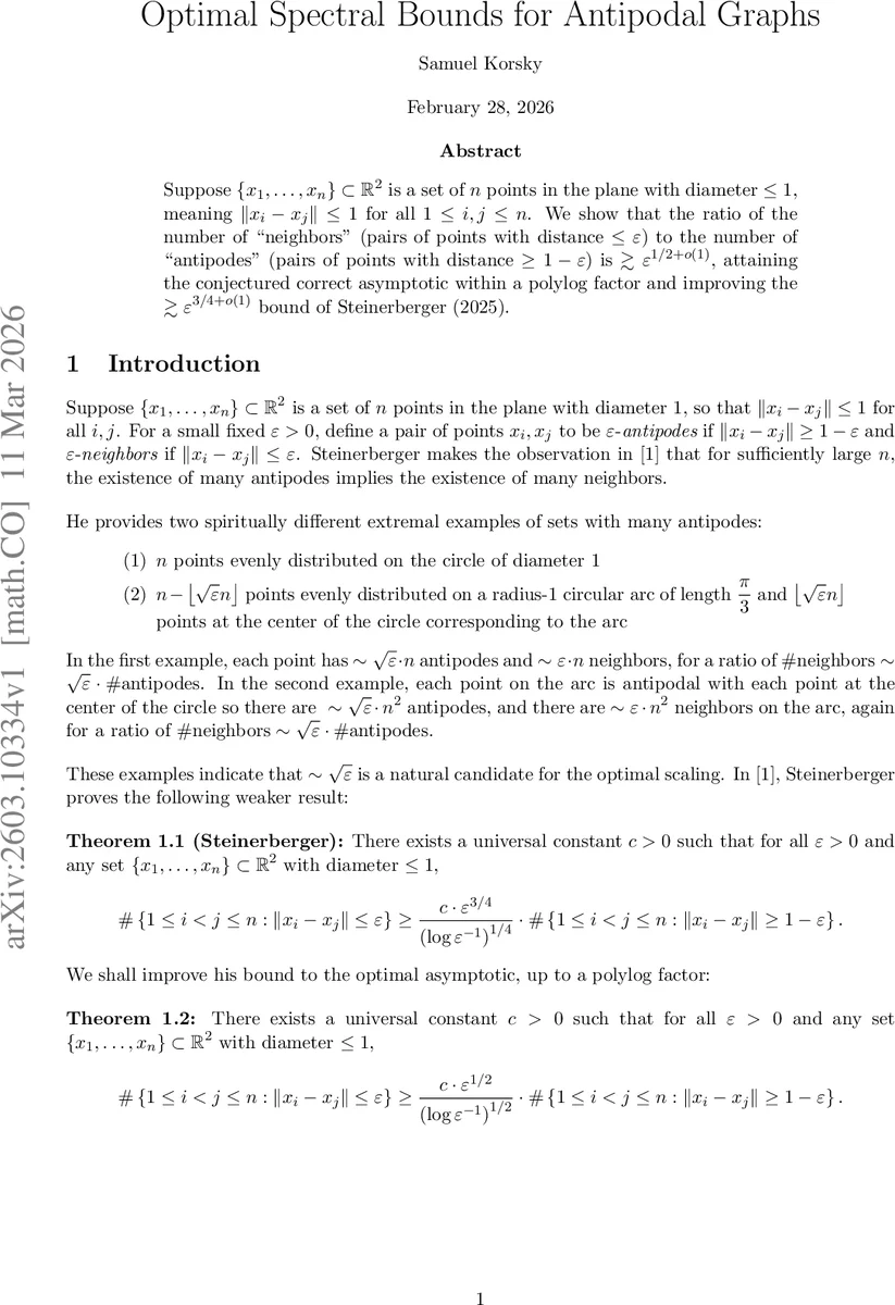
Suppose $\left{x_1, \dots, x_n\right} \subset \mathbb{R}^2$ is a set of $n$ points in the plane with diameter $\leq 1$, meaning $|x_i - x_j| \leq 1$ for all $1 \leq i,j \leq n$. We show that the ratio of the number of “neighbors” (pairs of points with distance $\leq \varepsilon$) to the number of “antipodes” (pairs of points with distance $\geq 1 - \varepsilon$) is $\gtrsim\varepsilon^{1/2 + o(1)}$, attaining the conjectured correct asymptotic within a polylog factor and improving the $\gtrsim\varepsilon^{3/4+o(1)}$ bound of Steinerberger (2025).

💡 Research Summary

The paper studies a finite set X = {x₁,…,xₙ} of points in the Euclidean plane whose diameter does not exceed 1. For a small parameter ε > 0 the authors distinguish two types of unordered pairs: ε‑neighbors (pairs whose distance is at most ε) and ε‑antipodes (pairs whose distance is at least 1 − ε). The central question, raised by Steinerberger (2025), is how many ε‑neighbors must be present once a certain number of ε‑antipodes are guaranteed. Steinerberger proved a lower bound of the form

 #neighbors ≥ c·ε^{3/4}(log ε)^{1/4}·#antipodes,

which matches the trivial examples up to a factor of ε^{−1/4}. He conjectured that the optimal exponent should be 1/2, i.e. #neighbors ≳ ε^{1/2}·#antipodes.

The authors improve this dramatically, establishing

 #neighbors ≥ c·ε^{1/2}(log (1/ε))^{1/2}·#antipodes,

which is optimal up to a polylogarithmic factor. The proof proceeds in several conceptual steps.

1. Geometric reduction to a graph.
   All extremal configurations can be assumed to lie within an ε‑neighbourhood of the boundary of the convex hull K of X. The boundary ∂K is discretised into k ≈ ε^{−1} arcs of length ε/2, each represented by a box B_i. A graph G = (V,E) – the “antipode graph’’ – is defined on these boxes: vertices i and j are adjacent if there exist points x∈B_i, y∈B_j with ‖x−y‖ ≥ 1 − ε. The adjacency matrix is denoted M.

2. Spectral bound via Collatz‑Wielandt.
   Instead of the classical trace bound λ₁(M) ≤ √{tr(MᵀM)} used by Steinerberger, the authors apply the Collatz‑Wielandt formula:

 λ₁(M) = max_{x>0} min_i (Mx)_i / x_i.

Choosing the positive vector x_i = √{d_i} (where d_i is the degree of vertex i) yields

 λ₁(M) ≤ max_i ∑{j∈N(i)} d_j / √{d_i} ≤ max_i ∑{j∈N(i)} d_j.

Thus the spectral radius is controlled by the sum of degrees of the neighbours of a vertex. To make λ₁(M) small, high‑degree vertices must have, on average, low‑degree neighbours.

3. Precise analysis of common neighbours.
   The key technical ingredient is a refined geometric lemma about the intersection of two thin annuli. Lemma 4.1 shows that if two annuli have inner radius 1 − ε, outer radius 1, and their centres are at distance d with 4ε ≤ d ≤ 1, then their intersection consists of two curvilinear quadrilaterals whose horizontal width is O(ε/d) and vertical height O(ε). Consequently the intersection can be covered by O(1/d) boxes of size ε/2 × ε/2. This improves the earlier estimate that required d ≳ √ε; the new bound works for all d ≳ ε.

4. Bounding the degree sum.
   For a fixed vertex i, let W be the set of vertices whose boxes lie within distance 100ε of B_i. Because the convex hull is thin, |W| is O(1). The contribution of W to ∑_{j∈N(i)} d_j is O(k). For the remaining vertices V \ W, the refined annulus lemma implies that the number of vertices having at least s common neighbours with i is at most c·k/s. Summing over s gives

 ∑_{j∈V\W} |N(i)∩N(j)| ≤ c·k·log k.

Since ∑{j∈N(i)} d_j = ∑{j∈V} |N(i)∩N(j)|, we obtain

 ∑_{j∈N(i)} d_j = O(k·log k).

Because k ≈ ε^{−1}, this yields

 λ₁(M) = O(ε^{−1/2}·(log (1/ε))^{1/2}).

5. From spectral radius to neighbor‑antipode ratio.
   A standard counting argument shows that if λ₁(M) = O(ε^{−α}), then the ratio #neighbors / #antipodes is at least a constant times ε^{α}. Substituting α = 1/2 gives the announced bound.

The paper therefore closes the gap left by Steinerberger, proving that the ε^{1/2} scaling is essentially optimal, up to a logarithmic factor. The novelty lies in replacing a global trace estimate with a local Collatz‑Wielandt bound and in extending the annulus intersection analysis to the full range d ≥ ε, which together enable the sharp spectral control. The result has immediate implications for geometric discrepancy problems and for understanding extremal configurations of points with prescribed distance constraints.