An operator-level ARCH Model

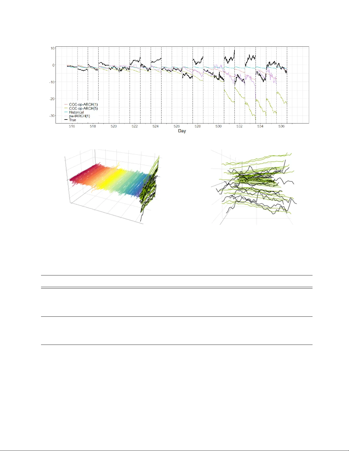
An op erator-lev el AR CH Mo del Alexander Aue 1 , Sebastian Kühnert 2 , Gregory Rice 3 , and Jerem y V anderDo es 4 1 Departmen t of Statistics, Univ ersity of California, Da vis, CA 95616 Da vis, USA, ‡ aaue@ucda vis.edu 2 Departmen t of Mathematics, Ruhr Universit y Bo c h um, 44780 Bo c h um, German y , * sebastian.kuehnert@ruhr-uni-b och um.de 3,4 Departmen t of Statistics and Actuarial Science, Univ ersit y of W aterlo o, ON N2L 0A4 W aterlo o, Canada, † grice@u waterloo.ca , Jerem y .V anderDo es@u waterloo.ca Marc h 15, 2026 Abstract AutoRegressiv e Conditional Heteroscedasticit y (AR CH) mo dels are standard for mo deling time series exhibiting v olatility , with a ric h literature in univ ariate and m ul- tiv ariate settings. In recent y ears, these mo dels hav e b een extended to function spaces. Ho wev er, functional ARCH and generalized ARCH (GARCH) pro cesses established in the literature ha ve th us far b een restricted to mo del “p oint wise” v ariances. In this pap er, w e prop ose a new AR CH framew ork for data residing in general separable Hilb ert spaces that accounts for the full evolution of the conditional cov ariance op erator. W e deﬁne a general op erator-level ARCH mo del. F or a simpliﬁed Constan t Conditional Correlation v ersion of the mo del, w e establish conditions under whic h suc h mo dels admit strictly and weakly stationary solutions, ﬁnite moments, and weak serial dep endence. Addition- ally , w e deriv e consistent Y ule–W alk er-t yp e estimators of the inﬁnite-dimensional mo del parameters. The practical relev ance of the mo del is illustrated through sim ulations and a data application to high-frequency cumulativ e intrada y returns. MSC 2020 subje ct classiﬁc ations: 60G10, 62F12, 62R10 Keywor ds: ARCH; ﬁnancial time series; functional data; parameter estimation; stationary solutions 1 (a) S&P 500 price curves (b) S&P 500 OCIDR Figure 1: S&P500 Data. Visualization of price (left) and o v ernigh t cumulativ e intrada y return (right) curv es based on 15-minute resolution S&P 500 sto c k market prices from 2018 to 2020 1 In tro duction Conditionally heteroscedastic pro cesses are fundamen tal in ﬁnancial modeling. T o cap- ture their dynamics, Engle ( 1982 ) introduced the A utor e gr essive Conditional Heter osc e dastic (AR CH) model, later extended b y Bollerslev ( 1986 ) to the Gener alize d ARCH (GARCH) mo del. Extensiv e reviews of uni- and m ultiv ariate (G)AR CH as well as other related volatil- it y mo dels can b e found in Andersen et al. ( 2009 ), Asai et al. ( 2006 ), Bauw ens et al. ( 2006 ), F rancq and Zakoïan ( 2019 ), and Gouriéroux ( 1997 ). With adv ances in data pro cessing and the gro wing av ailability of high-frequency ﬁnancial data, functional v olatility and (G)ARCH (f(G)ARCH) mo dels hav e gained prominence. As a motiv ating example, consider observing on consecutive da ys k ∈ { 1 , . . . , N } the price of the S&P 500 index at a resolution of one minute. Conv enien tly , these observ ations can b e view ed as a sample of curv es or functions { P k ( t ) , i ∈ { 1 , . . . , N } , t ∈ [0 , 1] } , where intrada y time is normalized to the unit in terv al; see the left panel of Figure 1 . A transformation of particular interest are the o vernigh t intrada y log-returns X k ( t ) = log P k ( t ) − log P k − 1 (1) ; see the right panel of Figure 1 . Represen tation of the data as functions constructed from noisy high-dimensional in traday observ ations allo ws for the use of tec hniques from functional data analysis. W e refer the reader to Horv áth and Kok oszk a ( 2012 ) and Hsing and Eubank ( 2015 ) for introductions to functional data analysis, and to Bosq ( 2000 ) and Bosq and Blanke ( 2007 ) for introductions to linear time series pro cesses in function spaces. In seminal w ork, Hörmann et al. ( 2013 ) in tro duced the fAR CH (1) pro cess to mo del conditional heteroscedasticit y in functional time series data. Their mo del w as extended to fGAR CH (1 , 1) b y Aue et al. ( 2017 ), and to general fGARCH ( p, q ) by Cero vec ki et al. ( 2019 ). F or further dev elopments and modiﬁed functional GAR CH and v olatility models, see Andersen et al. ( 2024 ), Kearney et al. ( 2023 ), Kühnert ( 2019 , 2020 ), Laksaci et al. ( 2025 ), 2 Li et al. ( 2025 ), Rice et al. ( 2023 ), Sun and Y u ( 2020 ). Henceforth, we refer to these existing mo dels as “p oint wise” f(G)ARCH (p w-f(G)AR CH) mo dels, since they are form ulated as follows: F or the function spaces C [0 , 1] and L 2 [0 , 1] of con tinuous and square-in tegrable functions on [0 , 1] , the pw-fAR CH ( p ) mo del as in tro duced in Cerov ec ki et al. ( 2019 ) takes the form X k ( t ) = σ k ( t ) ε k ( t ) , σ 2 k ( t ) = δ ( t ) + p X i =1 α i ( X 2 k − i )( t ) , k ∈ Z ; E ( ε 2 0 ( t )) = 1 . (1.1) Here, the mo del parameters are δ , a p ositive function, and α i , b ounded linear operators mapping non-negative functions to non-negative functions, with the ε k b eing i.i.d. and cen- tered inno v ations. When there exists a stationary and causal solution to ( 1.1 ) with ﬁnite second-order momen ts, the condition E ( ε 2 0 ( t )) = 1 iden tiﬁes σ 2 k ( t ) = V ar ( X k ( t ) |F k − 1 ) as the point wise conditional v ariance, where F k = σ ( ε i , i ≤ k ) is the information ﬁltration generated by the innov ations. Despite its success in numerous applications, this mo del has some limitations. First, it only explicitly mo dels the serial dep endence structure of the p oin twise conditional v ariance V ar ( X k ( t ) |F k − 1 ) . F or man y tasks, for example the construction of a prediction set for X k , one wishes to estimate the full conditional cov ariance kernel/operator of the sequence. Under mo del ( 1.1 ), so long as it is well-deﬁned, the conditional co v ariance k ernel takes the form Co v  X k ( t ) , X k ( s )   F k − 1  = E  X k ( t ) X k ( s )   F k − 1  = σ k ( t ) σ k ( s ) C ε ( t, s ) , where C ε is the co v ariance kernel of the inno v ations. As such, the conditional cov ariance forecast implied b y model ( 1.1 ) constitutes a “rank-one up date” to the cov ariance of the inno v ations, which ma y b e o v erly simplistic. Similar critiques of the multiv ariate diagonal GARCH mo del ha ve led to a plethora of al- ternativ e mo dels of v arying complexit y , including the VEC, CCC, DCC, and BEKK GARCH; see F rancq and Zak oïan ( 2019 , Ch. 10). Analogues of these mo dels for functional time series ha ve not b een considered, to the best of our knowledge. One p otential reason for this is the fact that the iden tity map is not compact in general, separable Hilb ert spaces; an issue that is circumv en ted in the form ulation of p w-fAR CH mo dels. The non-compactness of the iden tity map prev ents the user from sp ecifying in a useful wa y an innov ation pro cess with iden tity cov ariance so that the conditional cov ariance of the mo del, and the mo del param- eters, can b e iden tiﬁed. This identiﬁabilit y issue can b e ov ercome, how ev er, b y sp ecifying that the innov ations p ossess some kno wn, injective co v ariance op erator, which is a critical idea underlying our mo del. In this pap er, we prop ose a new ARCH mo del, termed “op erator-level AR CH”, in general separable Hilb ert spaces. It provides a more direct generalization of AR CH pro cesses to the functional setting in that the mo del is formulated directly for the conditional co v ariance op erator, rather than the p oin t wise v ariance as with p w-fARCH mo dels. Since the general 3 mo del is, from a theoretical p oin t of view, quite c hallenging, w e fo cus on an op erator-lev el coun terpart of the Constant Conditional Corr elation (CCC) AR CH mo del in the m ultiv ari- ate setting, whic h is more feasible. W e establish conditions on the mo del parameters and inno v ations suc h that it admits strictly and weakly stationary solutions, reﬁning the classical notion of the (functional) top Lyapunov exp onent for strict stationarit y to suit our general setting. A dditionally , w e provide suﬃcient conditions for the existence of ﬁnite momen ts and w eak dep endence. Our estimation approach targets the AR CH op erators under kno wn orders and relies on pseudo Y ule–W alk er (YW) equations. W e derive consisten t YW esti- mators for the in tercept term ∆ , which is a self-adjoint and p ositiv e deﬁnite op erator in our setting, and the op erators α i , which map b etw een op erator spaces. The estimates are devel- op ed under a sp eciﬁc diagonal represen tation in ﬁnite- and inﬁnite-dimensional settings. The iden tiﬁability issue that arises when directly deriving the YW-t yp e equations are addressed using speciﬁc transformations of the data. In the inﬁnite-dimensional case, w e in tro duce a Sob olev-t yp e condition inspired by Hall and Meister ( 2007 ) to quan tify the appro ximability of inﬁnite-dimensional op erators by their ﬁnite-dimensional approximations. The estimation is conducted via Tikhonov-t yp e pseudoin v erses in the YW framew ork. While the theoretical prop erties of the estimators are well established, their complexit y may presen t practical c hal- lenges. The applicabilit y of the prop osed metho dology is illustrated through a simulation study an application to in traday log-returns. The structure of the pap er is as follows. Section 2 in tro duces the general mo del and out- lines the main assumptions. Section 3 introduces the corresp onding CCC mo del and deriv es stationarit y conditions and probabilistic prop erties. Section 4 addresses parameter estima- tion. Section 5 presen ts a simulation study and Section 6 pro vides applications. Section 7 concludes. A dditionally , the app endix contains preliminaries (Sections A and B ), and pro ofs of key results (Section C ). W e adopt the follo wing notation. The iden tity map is denoted by I . On a Cartesian pro duct space V n , n ∈ N , we deﬁne inner pro duct and norm by ⟨ x, y ⟩ = P n i =1 ⟨ x i , y i ⟩ and ∥ x ∥ 2 = P n i =1 ∥ x i ∥ 2 for x = ( x 1 , . . . , x n ) ⊤ , y = ( y 1 , . . . , y n ) ⊤ ∈ V n , assuming V has inner pro duct ⟨· , ·⟩ and norm ∥ · ∥ . The spaces of b ounded linear, Hilbert-Schmidt (H-S), and n uclear/trace-class operators from H to H ⋆ are resp ectively denoted by L H , H ⋆ , S H , H ⋆ , and N H , H ⋆ , with norms ∥ · ∥ L , ∥ · ∥ S , ∥ · ∥ N and H-S inner pro duct ⟨· , ·⟩ S . When H , H ⋆ are clear, w e write T for T H , H ⋆ and T H : = T H , H , where T ∈ {L , S , N } . F or A ∈ L , A ∗ denotes the adjoin t. W rite T ≥ 0 ( T > 0 ) for the self-adjoin t non-negativ e (p ositiv e) deﬁnite elemen ts of T . F or x ∈ H , y ∈ H ⋆ , the tensor pr o duct op er ator is x ⊗ y : = ⟨ x, ·⟩ y , with x ⊗ 2 : = x ⊗ x, and x ⊗ S y is used when x, y are H-S op erators. F or p ∈ [1 , ∞ ) , L p H = L p H (Ω , A , P ) is the space of X ∈ H with E ∥ X ∥ p < ∞ . The cr oss-c ovarianc e op er ator is C X,Y : = E [ X − E X ] ⊗ [ Y − E Y ] , X ∈ L 2 H , Y ∈ L 2 H ⋆ , and the c ovarianc e op er ator is C X = C X,X , with exp ectation in the Bo chner sense. F or w eakly stationary X = ( X k ) and join tly weakly stationary X , Y , the lag- h -c ovarianc e and 4 lag- h -cr oss-c ovarianc e op erators are C h X : = C X 0 ,X h and C h X , Y : = C X 0 ,Y h , with C X : = C 0 X and C X , Y : = C 0 X , Y . F urther, X = ( X k ) is a we ak white noise (WWN) if it is w eakly stationary , cen tered, with E ∥ X 0 ∥ 2 > 0 , and C h X = 0 for all h  = 0 ; and a str ong white noise (SWN) is an i.i.d. WWN. F or sequences ( b n ) , ( c n ) ⊂ R , b n ≍ c n (as n → ∞ ) denotes asymptotic equiv alence up to constan ts. Unless stated otherwise, all limits are taken as N → ∞ . 2 General mo del and assumptions Let H b e a separable Hilb ert space equipp ed with the inner pro duct ⟨· , ·⟩ . Deﬁnition 2.1 . W e call ( X k ) k ∈ Z ⊂ H an op er ator-level AR CH ( p ) pr o c ess (op-ARCH ( p ) ) if X k = Σ 1 / 2 k ( ε k ) , Σ k = ∆ + p X i =1 α i ( X ⊗ 2 k − i ) , k ∈ Z , (2.1) where ε = ( ε k ) is a SWN with cov ariance op erator C ε , p ∈ N , ∆ ∈ S > 0 , and α i : S → S are b ounded linear op erators with α i : S ≥ 0 → S ≥ 0 for all i = 1 , 2 , . . . , p, with α p  = 0 . As in the p w-fARCH framew ork, w e call the parameter ∆ the in tercept term, and the parameters α 1 , . . . , α p the (op-)AR CH op erators. Here, ∆ is a deterministic, self-adjoint, p ositiv e deﬁnite H-S op erator, and each α i is a b ounded and linear op erator mapping H-S to H-S op erators, preserving self-adjoin tness and non-negative deﬁniteness. As a consequence, Σ k is self-adjoint and p ositiv e deﬁnite. If ( 2.1 ) admits a strictly stationary solution with ﬁnite second momen ts, then E  X ⊗ 2 k   F k − 1  = Σ 1 / 2 k C ε Σ 1 / 2 k , k ∈ Z , (2.2) so that the pro cess exhibits conditional heteroscedasticit y . Note that the mo del remains w ell-deﬁned if ∆ is merely b ounded linear rather than H-S, but since consistent estimation from ﬁnite samples requires compactness, we keep the sligh tly stronger H-S assumption. The form ula ( 2.2 ) highligh ts the standard iden tiﬁabilit y issue in GAR CH mo dels: neither Σ k nor its deﬁning parameters are uniquely determined by ( 2.2 ), since unitary transformations of Σ k and C ε lea ve the conditional cov ariance unc hanged. In multiv ariate GAR CH mo dels this is av oided by imp osing C ε = I , iden tifying Σ k as the conditional cov ariance op erator. In inﬁnite-dimensional Hilb ert spaces, ho wev er, the iden tity map I is not compact and this is not feasible. Instead, if C ε is an y known injectiv e co v ariance op erator, then ( 2.2 ) uniquely iden tiﬁes Σ k . Hence, throughout we assume: Assumption 2.1. The c ovarianc e op er ator C ε is known and inje ctive. When for example H = L 2 [0 , 1] , and C ε ( f )( t ) = Z 1 0 C ε ( t, s ) f ( s ) ds, 5 for a cov ariance k ernel C ε , natural choices satisfying the ab ov e are Brownian motion errors, where C ε ( t, s ) = σ 2 min { t, s } , and Ornstein–Uhlen b ec k errors, where C ε ( t, s ) = σ exp( − θ | t − s | ) . Although the conditional cov ariance op erator do es not coincide with Σ k , it can b e easily reco vered from it using the kno wn C ε . In pw-f(G)AR CH mo dels of higher order, Mark ovian state-space forms ha v e b een used to establish stationarity (cf. Cerov ec ki et al. 2019 , Kühnert 2020 ). Our op-AR CH ( p ) pro cess also admits a Marko vian representation, though in a more in tricate form: X ⊗ 2 , [ p ] k = Υ k  ∆ + Ψ ( X ⊗ 2 , [ p ] k − 1 )  , k ∈ Z . (2.3) Here X ⊗ 2 , [ p ] k collects the past p “squared” functions, so X ⊗ 2 , [ p ] k : =  X ⊗ 2 k , X ⊗ 2 k − 1 , . . . , X ⊗ 2 k − p +1  ⊤ , (2.4) with constant p art ∆ : = (∆ , 0 , . . . , 0) ⊤ , Ψ : S p ≥ 0 → S p ≥ 0 refers to the op erator-v alued matrix Ψ : =        α 1 · · · · · · · · · α p I 0 · · · · · · 0 0 I 0 · · · 0 . . . . . . . . . . . . . . . 0 · · · 0 I 0        , (2.5) and Υ k : S p ≥ 0 → S p ≥ 0 refers to the map deﬁned b y Υ k ( A ) : = ( A 1 / 2 1 ε ⊗ 2 k A 1 / 2 1 , A 2 , . . . , A p ) ⊤ for A = ( A 1 , . . . , A p ) ⊤ . Although the represen tation ( 2.3 ) is natural, establishing stationarit y is challenging: the nonlinearit y of Υ k rules out the use of a top Lyapuno v exp onent (cf. Kingman 1973 , Liggett 1985 ), and the geometric momen t con traction condition of W u and Shao ( 2004 ), as employ ed in Hörmann et al. ( 2013 ) for pw-fAR CH mo dels, do es not app ear applicable to the transformation A 7→ Υ k ( ∆ + Ψ ( A )) . Nevertheless, a strictly stationary solution can still b e constructed algorithmically (see F rancq and Zak oïan 2019 , p. 289 for the v ech (G)AR CH case). A more tractable mo del that is amenable to theoretical analysis will b e introduced b elo w. Sev eral of the results b elow, including crucially metho ds to estimate the op erators in ( 2.1 ), are simpliﬁed considerably b y assuming the following: Assumption 2.2. C ε c ommutes with Σ k in ( 2.1 ) for al l k . Assumptions 2.1 – 2.2 imply that ∆ and the ranges of α 1 , . . . , α p are diagonalizable with resp ect to the (kno wn) eigenbasis of C ε . In ﬁnite-dimensional (G)ARCH mo dels, this is t ypically ensured b y taking C ε = I . The c hoice of C ε ma y th us b e viewed as selecting the basis that diagonalizes the conditional co v ariance. In the results b elow, we explicitly state whic h arguments rely on this assumption. Moreov er, to delve more deeply into the structure 6 of the op-ARCH mo del, and provide comparisons to other multiv ariate GARCH mo dels, w e use the notation α : S p ≥ 0 → S ≥ 0 , A = ( A 1 , . . . , A p ) ⊤ 7→ α ( A ) = p X i =1 α i ( A i ) , (2.6) and assume the following. Assumption 2.3. The op er ator α is H-S. Let ( e j ) ∞ j =1 b e the eigenbasis asso ciated to the co v ariance op erator C ε . Assumption 2.3 , together with the fact that the space of H-S op erators from S p to S is a separable Hilb ert space yields α = p X i =1 ∞ X j =1 ∞ X k =1 ∞ X ℓ =1 ∞ X m =1 a ij k ℓm  E ij k ⊗ S ( e ℓ ⊗ e m )  , (2.7) where E ij k is the vector placing e j ⊗ e k at p osition i and zeros elsewhere. By the deﬁnitions of Σ k in the op-AR CH ( p ) equation and α , and with a ij ℓ : = a ij j ℓℓ , this leads to the simpliﬁed represen tation α = p X i =1 ∞ X j =1 ∞ X ℓ =1 a ij ℓ  E ij j ⊗ S ( e ℓ ⊗ e ℓ )  . (2.8) Eac h comp onent α i of α maps S ≥ 0 to S ≥ 0 , i.e. non-negative deﬁnite, self-adjoin t H-S op era- tors in to itself. Thus, for any A = ( A 1 , . . . , A p ) ⊤ ∈ S p ≥ 0 , α ( A ) is self-adjoin t and non-negativ e deﬁnite under mild conditions. T o establish the latter, note that we need  α ( A )( x ) , x  = p X i =1 ∞ X j =1 ∞ X ℓ =1 a ij ℓ ⟨ A i ( e j ) , e j ⟩⟨ x, e ℓ ⟩ 2 ≥ 0 , x ∈ H . Since ⟨ A i ( e j ) , e j ⟩ ≥ 0 for all i, j , a suﬃcien t condition for α ( A ) to b e non-negativ e deﬁnite is a ij ℓ ≥ 0 for all i, j, ℓ. 3 CCC-op-AR CH mo del and structure As indicated ab o ve, w e now in tro duce a more parsimonious mo del. The expansion ( 2.8 ) is the most general form of the op-AR CH op erators satisfying Assumption 2.2 . In analogy to m ultiv ariate GARCH, this is akin to a “VEC-ARCH” sp eciﬁcation (see F rancq and Zakoïan 2019 , Ch. 10.2.2). Although such a mo del allows for a ﬂexible serial dep endence structure, it is often considered ov erparameterized, c hallenging to estimate, and theoretically diﬃcult to analyze. A more tractable mo del is obtained b y retaining only the diagonal terms in ( 2.8 ). This section is devoted to the discussion of such a mo del, where Assumptions 2.1 – 2.3 hold. 7 Deﬁnition 3.1 . W e say that a pro cess ( X k ) k ∈ Z is a Constant Conditional Corr elation op er ator- level ARCH ( p ) (CCC-op-AR CH ( p ) ) pro cess if ( 2.1 ) holds with α = p X i =1 ∞ X ℓ =1 a iℓℓ  E iℓℓ ⊗ S ( e ℓ ⊗ e ℓ )  . (3.1) This is called a “CCC” mo del since it assumes that α only dep ends on the diagonal-terms in its expansion, while the comp onen ts of the pro cess X i remain “conditionally correlated” through their common dep endence on C ε . W e note that one migh t also consider a CCC mo del of the form ( 2.1 ) where for a compact cov ariance operator G , Σ k = H 1 / 2 k G H 1 / 2 k , and H k satisﬁes the recursion on the right-hand side of ( 2.1 ). Under the commutativit y Assumption 2.2 and with α following ( 3.1 ), this reduces to the giv en CCC mo del. Throughout this section, ( X k ) is assumed to b e a CCC-op-ARCH ( p ) mo del for some p ∈ N . One of the b eneﬁts of this mo del is that there exists a linear Marko vian form asso ciated with it. T o b e precise, w e ha v e (see also Example B.1 ) X ⊗ 2 , [ p ] k, d = ∆ k + Ψ k  X ⊗ 2 , [ p ] k − 1 , d  , k ∈ Z , (3.2) where X ⊗ 2 , [ p ] k, d is the diagonal part of X ⊗ 2 , [ p ] k in ( 2.4 ), whic h is for each comp onent deﬁned b y X ⊗ 2 k − i +1 , d : = ∞ X ℓ =1 ⟨ X k − i +1 , e ℓ ⟩ 2 ( e ℓ ⊗ e ℓ ) , i ∈ { 1 , ..., p } , k ∈ Z . (3.3) Here ∆ k : = ( ψ k (∆) , 0 , . . . , 0) ⊤ , and Ψ k has the same form as Ψ in ( 2.5 ) with eac h α i replaced b y ψ k ◦ α i , where ◦ refers to comp osition, and ψ k ( B ) : = ∞ X j =1 ⟨ ε k , e j ⟩ 2 b j ( e j ⊗ e j ) , for B = ∞ X j =1 b j ( e j ⊗ e j ) ∈ S ≥ 0 . (3.4) It should b e noted that a host of other p oten tial, simpliﬁed mo dels starting from ( 2.8 ) migh t b e considered. F or ease of presentation and due to the empirical p erformance of the CCC-op-AR CH ( p ) mo del in our analyses b elow, we hav e c hosen to fo cus on this case. W e discuss this and av en ues for future research in Section 7 . 3.1 Strict stationarit y T o deduce conditions under which this mo del admits a stationary solution, w e in tro duce a top Lyapunov exp onent (cf. Kingman 1973 , Liggett 1985 ). T o this end, w e deﬁne τ : B S p ≥ 0 , d → [0 , ∞ ) , τ ( B ) : = sup ∥ A ∥ S p ≤ 1 , A ∈S p ≥ 0 , d ∥ B ( A ) ∥ S , (3.5) 8 where S ≥ 0 , d ⊂ S ≥ 0 denotes the subset of non-negativ e, self-adjoint H-S op erators with the diagonal form A = P j a j ( e j ⊗ e j ) , and B S p ≥ 0 , d the set of bound ed linear op erators on S ≥ 0 , d . Although the functional τ do es not deﬁne a norm, it satisﬁes several useful prop erties for our analysis. It is dominated b y the op erator norm, τ ( B ) ≤ ∥ B ∥ L , compatible with the H-S norm so that ∥ B ( A ) ∥ S ≤ τ ( B ) ∥ A ∥ S , and sub-m ultiplicative, τ ( B 1 ◦ B 2 ) ≤ τ ( B 1 ) τ ( B 2 ) . Prop osition 3.1. The top Ly apunov exp onent deﬁne d by γ : = lim k →∞ 1 k ln τ  Ψ k ◦ Ψ k − 1 ◦ · · · ◦ Ψ 1  = lim k →∞ 1 k E ln τ  Ψ k ◦ Ψ k − 1 ◦ · · · ◦ Ψ 1  , (3.6) exists with γ ∈ [ −∞ , ∞ ) , wher e the ﬁrst limit holds almost sur ely. Mor e over, γ = inf k ∈ N 1 k E ln τ  Ψ k ◦ Ψ k − 1 ◦ · · · ◦ Ψ 1  . (3.7) Theorem 3.1. If γ < 0 , (3.8) the CCC-op-ARCH ( p ) pr o c ess ( X k ) admits a strictly stationary, c ausal, and almost sur ely unique solution. The same holds for the asso ciate d pr o c ess (Σ k ) . The condition ( 3.8 ) is diﬃcult to v erify in practice, ev en with known, relatively simple, op erators α 1 , ..., α p . The follo wing tw o suﬃcient conditions are more tractable. Prop osition 3.2. Condition ( 3.8 ) is satisﬁe d if, for some n ∈ N and ν > 0 , E τ ν  Ψ n ◦ Ψ n − 1 ◦ · · · ◦ Ψ 1  < 1 . (3.9) Mor e explicitly, ( 3.9 ) is satisﬁe d with n = p and ν = 1 if ∥ α ∥ L E ∥ ε 0 ∥ 2 p X ℓ =1 ℓ  ∥ α ∥ L E ∥ ε 0 ∥ 2  p − ℓ < 1 . (3.10) Remark 3.1. (a) In contrast to real-v alued (G)ARCH pro cesses (cf. F rancq and Zakoïan 2019 , Theorem 2.4), the condition ( 3.8 ) is not necessary , since norms on inﬁnite-dimensional spaces are not equiv alent (cf. Cerov ec ki et al. 2019 , Remark 1). (b) The suﬃcient condition ( 3.10 ) is conv enien t, but relatively crude. A sharp er analysis of this constrain t may further relax the requirement, which we do not pursue here. F urther, as each Ψ k con tains iden tity maps—and hence has norm at least 1 —( 3.10 ) can, by the deﬁnition of Ψ k , only hold for comp ositions Ψ n ◦ Ψ n − 1 ◦ · · · ◦ Ψ 1 with n ≥ p (see the pro of in Section C ). F or simplicity , we fo cus on the case n = p . 9 Example 3.1 . Suppose p = 1 . Then considering ( 3.9 ) with n = 1 leads to the suﬃcient stationarit y condition E  sup j ≥ 1 a ν 1 j j ⟨ ε 1 , e j ⟩ 2 ν  < 1 , for some ν > 0 . Moreo v er, one may see from this that E τ ν  Ψ 1  ≤ ∥ α 1 ∥ ν L E  sup j ≥ 1 ⟨ ε 1 , e j ⟩ 2 ν  . With ν = 1 , this leads to the suﬃcient condition ∥ α 1 ∥ L ∥ C ε ∥ L < 1 . 3.2 Existence of momen ts, w eak dep endence, and weak stationarit y Under suitable conditions, CCC-op-AR CH pro cesses p ossess ﬁnite moments and displa y w eak serial dep endence. In particular, they are L p - m -appro ximable, a weak dep endence notion for functional data initially introduced in Hörmann and Kok oszk a ( 2010 ). A pro cess ( Y k ) k ∈ Z ⊂ H is L p - m -appr oximable if (a) it admits a Bernoulli shift representation, i.e. Y k = f ( ε k , ε k − 1 , . . . ) for some i.i.d. sequence ( ε k ) k ∈ Z taking v alues in a measurable space S , and a measurable mapping f : S N → H , and (b) with Y ( m ) k : = f ( ε k , . . . , ε k − m +1 , ε ′ k − m , ε ′ k − m − 1 , . . . ) , where ( ε ′ k ) k ∈ Z is an indep endent sequence of copies of ε 0 , and with ξ Y ,p ( m ) = ( E ∥ Y 0 − Y ( m ) 0 ∥ p H ) 1 /p , ∞ X m =1 ξ Y ,p ( m ) < ∞ . (3.11) A ccording to (a), L p -m-appro ximable pro cesses are strictly stationary and ergo dic. If ( 3.11 ) holds with p ≥ 2 , then the pro cess Y k satisﬁes for example the cen tral limit theorem. This condition is satisﬁed b y man y standard mo dels, including functional AR and linear processes (as illustrated in Hörmann and K ok oszk a 2010 ), and also p w-(G)ARCH mo dels. The fol- lo wing result pro vides suﬃcien t conditions for this prop erty and for the existence of ﬁnite momen ts. In this result, the notation ∥ · ∥ 4 app ears, referring to the norm of Schatten class op er ators of or der 4 (see Section A ). Prop osition 3.3. L et ( 3.9 ) and ( ε k ) ⊂ L 2 ν H for the same ν hold. Then: (a) E ∥ X ⊗ 2 0 ∥ ν S = E ∥ X 0 ∥ 2 ν < ∞ and E ∥ Σ 1 / 2 0 ∥ 2 ν 4 = E ∥ Σ 0 ∥ ν S < ∞ . (b) The pr o c esses X k and Σ 1 / 2 k ar e L 2 ν - m -, and Y k = X ⊗ 2 k and Y k = Σ k ar e L ν - m - appr oximable, e ach with ge ometric al ly de c aying appr oximation err ors, i.e. ξ X, 2 ν ( m ) ≤ c † ρ m and ξ Y ,ν ( m ) ≤ c † ρ m for some c † > 0 and ρ ∈ (0 , 1) . 10 Prop osition 3.4. L et ( X k ) b e a we akly stationary CCC-op-ARCH ( p ) pr o c ess. Then, ( X k ) is a we ak white noise. F urther, µ Σ : = E (Σ 0 ) = E (Σ k ) for al l k , with µ Σ = ∆ + p X i =1 α i ( C X ) . (3.12) In addition, if Assumption 2.2 and also      p X i =1 α i ( C ε )      L < 1 (3.13) ar e satisﬁe d, then µ Σ has the mor e explicit r epr esentation µ Σ =  I − p X i =1 α i ( C ε )  − 1 (∆) . (3.14) Remark 3.2. (a) Eq. ( 3.14 ) p ar al lels the classic al formula for the unc onditional varianc e of univariate (G)AR CH mo dels (cf. F r anc q and Zakoïan 2019 ). Mor e over, ( 3.13 ) may stil l hold even when P p i =1 ∥ α i ∥ L ≥ 1 , sinc e ∥ C ε ∥ L < 1 for most r elevant innovation pr o c esses (e.g., the standar d Br ownian motion). (b) The moment c ondition in Pr op osition 3.3 for ν ≤ 1 is state d only for c ompleteness and is r e dundant, sinc e ﬁnite se c ond moments of ε 0 wer e alr e ady assume d. 3.3 Examples W e illustrate the ab ov e results with tw o classes of op-AR CH pro cesses on H = L 2 [0 , 1] , where ( ε k ) denotes an i.i.d. sequence of standard Brownian motions on [0 , 1] . Example 3.2 . Let p ∈ N . Consider the integral op erator ∆ with kernel min( t, s ) , s, t ∈ [0 , 1] , and deﬁne α i ( A ) = a i A for A ∈ S and scalars a i ≥ 0 for 1 ≤ i < p, and a p  = 0 . Then ∆ ∈ S > 0 and each α i ∈ L S maps S ≥ 0 to S ≥ 0 . (a) Let p = 1 . Since E ∥ ε 0 ∥ 2 = ∥ C ε ∥ N = 1 / 2 and ∥ α ∥ L = a 1 , condition ( 3.10 ) holds whenev er a 1 < 2 . In this case, Prop osition 3.3 yields E ∥ X 0 ∥ 2 < ∞ and E ∥ Σ 0 ∥ S < ∞ , so ( X k ) is w eakly stationary , a WWN by Prop osition 3.4 , and L 2 - m -appro ximable. (b) Let p = 3 . Here, ∥ α ∥ L ≤ a : = a 1 + a 2 + a 3 . Hence, ( 3.10 ) is satisﬁed if a ( a 2 + 4 a + 12) < 8 , whic h holds roughly for a ≤ 0 . 551 . 11 Example 3.3 . In the following, let ∆ = ∞ X ℓ =1 d ℓ ( e ℓ ⊗ e ℓ ) , α i = ∞ X ℓ =1 a iℓℓ ( e ℓ ⊗ e ℓ ) ⊗ S ( e ℓ ⊗ e ℓ ) , 1 ≤ i ≤ p, where ( d ℓ ) and ( a iℓℓ ) ℓ are p ositive, strictly decreasing, square-summable sequences. Then Σ k = ∞ X ℓ =1 Z k,ℓ ( e ℓ ⊗ e ℓ ) , X k = ∞ X ℓ =1 Z 1 / 2 k,ℓ ⟨ ε k , e ℓ ⟩ e ℓ , with Z k,ℓ = d ℓ + p X i =1 a iℓℓ Z k − i,ℓ ⟨ ε k − i , e ℓ ⟩ 2 . T o highligh t structural asp ects, let p = 1 and assume a 1 ℓℓ = aℓ − 2 for some a > 0 . Then ∥ α ∥ L E ∥ ε 0 ∥ 2 = sup ℓ ≥ 1 | a 1 ℓℓ | / 2 = a/ 2 , so, b y Example 3.2 , ( X k ) is strictly stationary , L 2 - m -appro ximable, and a WWN when a < 2 . F urther in this case Assumption 2.2 and ( 3.13 ) hold. Th us, by Prop osition 3.4 , µ Σ =  I − α 1 ( C ε )  − 1 (∆) . 4 Estimation in the CCC-op-AR CH mo del W e no w turn to the estimation of the parameters α 1 , ..., α p , and ∆ in the CCC-op-ARCH ( p ) . Henceforth, X = ( X k ) ⊂ H refers to a stationary CCC-op-AR CH ( p ) pro cess that p ossesses ﬁnite second momen ts from which we ha ve observ ed a stretch of length N , X 1 , ..., X N . W e will assume throughout the remainder of this article that Assumption 2.2 holds so that C ε and Σ k comm ute. Under this assumption, µ Σ = E (Σ k ) , C X = E ( X ⊗ 2 k ) = µ Σ C ε , Σ 1 / 2 k C ε Σ 1 / 2 k = Σ k C ε , k ∈ Z , and the op-AR CH equations imply that X ⊗ 2 k − C X = Σ 1 / 2 k ( ε ⊗ 2 k − C ε )Σ 1 / 2 k +  p X i =1 α i ( X ⊗ 2 k − i − C X )  C ε . (4.1) If w e calculate the cov ariances of the ab ov e with X ⊗ 2 k − i , 1 ≤ i ≤ p , due to causalit y the co v ariance with the ﬁrst term on the righ t-hand side of ( 4.1 ) will v anish, and the cov ariances 12 with the second term ma y b e expressed in terms of the α op erators. In order to shift the n uisance op erator C ε oﬀ of the terms containing the α ’s, we pro ceed ﬁrst b y applying on the righ t a Tikhonov -regularized inv erse C † ε : = ( C ε + ϑ N I ) − 1 , (4.2) where I denotes the iden tity map and ϑ N > 0 is an asymptotically v anishing regularization parameter, i.e., ϑ N → 0 . After this regularization, we also pro ject onto a ﬁnite-dimensional space. Let ( a j , e j ) b e the eigenpairs of C ε , i.e. a 1 ≥ a 2 ≥ · · · > 0 are the eigenv alues asso ciated with the eigenfunctions e 1 , e 2 , . . . of C ε . Then, the pro jection op erator on to the linear space spanned b y e 1 , . . . , e K , K ∈ N , is denoted by ` e K e 1 , and w e deﬁne C ‡ ε : = C ε C † ε . A ccording again to ( 4.1 ),  X ⊗ 2 k − C X  C † ε e K a e 1 = Σ 1 / 2 k ( ε ⊗ 2 k − C ε )Σ 1 / 2 k C † ε e K a e 1 +  p X i =1 α i ( X ⊗ 2 k − i − C X )  C ‡ ε e K a e 1 . (4.3) F urther, let X ⊗ 2 ε = ( X ⊗ 2 k, ε ) k ∈ Z ⊂ S and X ⊗ 2 , [ p ] = ( X ⊗ 2 , [ p ] k ) k ∈ Z ⊂ S p b e the pro cesses deﬁned b y X ⊗ 2 k, ε : = X ⊗ 2 k C † ε e K a e 1 , and X ⊗ 2 , [ p ] k : = ( X ⊗ 2 k , . . . , X ⊗ 2 k − p +1 ) ⊤ , k ∈ Z , (4.4) and their cen tered versions by ˜ X ⊗ 2 k, ε : = X ⊗ 2 k, ε − C X C † ε e K a e 1 , and ˜ X ⊗ 2 , [ p ] k : = X ⊗ 2 , [ p ] k − ( C X , . . . , C X ) ⊤ , k ∈ Z . (4.5) W e see according to ( 4.3 ) that the lag-1 cross-cov ariance op erators D = D K,N = C 1 X ⊗ 2 , [ p ] , X ⊗ 2 ε ∈ N S p , S satisfy the follo wing Y ule–W alker (YW)-type equation: D = α C + R , (4.6) where C = C X ⊗ 2 , [ p ] ∈ N S p , (4.7) with α from ( 2.6 ), and where the remainder R = R K,N is deﬁned b y R : = E  ˜ X ⊗ 2 , [ p ] 0 , ·  S " h α  ˜ X ⊗ 2 , [ p ] 0  i  C ‡ ε e K a e 1 − I  # . (4.8) 13 Notice that all the op erators in the YW-t yp e equation ( 4.6 ) are w ell-deﬁned due to causality of the in volv ed pro cesses and Prop osition 3.3 . If the remainder term is small, it seems natural in view of ( 4.6 ) to estimate α by ˆ D ˆ C − 1 . This, ho wev er, do es not yield a useful estimate, as α is not identiﬁable from α C when C is not injectiv e. F or example, in H = L 2 [0 , 1] with p = 1 , the op erator J ∈ S with k ernel j ( s, t ) = − 1 if s ≤ t and j ( s, t ) = 1 otherwise, satisﬁes ⟨ C ( K ) , K ⟩ S = 0 . This issue parallels the multiv ariate case where, for X ∈ R d , vec ( X X ⊤ ) ∈ R d 2 do es not hav e a full-rank co v ariance matrix, while the “half-vectorization” vec h ( X X ⊤ ) ∈ R d ( d +1) / 2 t ypically do es. In what follows, we derive estimators for the CCC-op-ARCH ( p ) op erators, that is, to reiterate, α in ( 2.8 ) satisﬁes α = p X i =1 ∞ X ℓ =1 a iℓℓ  E iℓℓ ⊗ S ( e ℓ ⊗ e ℓ )  , (4.9) based on the YW-t yp e equation ( 4.6 ), suitably mo diﬁed to ensure iden tiﬁability , as w ell as estimators for the intercept term ∆ . 4.1 Finite-dimensional setting Although our ultimate goal is to derive consisten t estimators for the inﬁnite-dimensional op erators in ( 4.9 ), w e b egin with estimating the CCC-op-ARCH op erators α 1 , . . . , α p , under the simplifying assumption that α = α K : = p X i =1 K X ℓ =1 a iℓℓ [ E iℓℓ ⊗ S ( e ℓ ⊗ e ℓ )] (4.10) for a ﬁnite in teger K . F urther, we assume that the observed curves X i are ﬁnite-dimensional, so that with X k,i = ⟨ X k , e i ⟩ : X k = K X i =1 X k,i e i , k ∈ Z . (4.11) The representation of X k yields with X k,ij : = X k,i X k,j : X ⊗ 2 k = K X i =1 K X j =1 X k,ij ( e i ⊗ e j ) , implying that eac h X ⊗ 2 , [ p ] k , with p ∈ N , is characterized b y the blo c k matrix   X k,ij  K i,j =1 ,  X k − 1 ,ij  K i,j =1 , . . . ,  X k − p +1 ,ij  K i,j =1  ⊤ ∈ R pK × K . 14 Throughout, the map diag : R K → R K × K and its adjoint diag ∗ : R K × K → R K construct a diagonal matrix from a vector and create a vector b y extracting the diagonal of the input matrix, resp ectively . Note that diag : R pK → R pK × K and diag ∗ : R pK × K → R pK are also comp onen t-wise deﬁned, i.e. for an y v ectors x 1 , . . . , x p ∈ R K and matrices A 1 , . . . , A p ∈ R K × K , diag( x 1 , . . . , x p ) : =  diag( x 1 ) , . . . , diag ( x p )  ⊤ , and diag ∗ ( A 1 , . . . , A p ) : =  diag ∗ ( A 1 ) , . . . , diag ∗ ( A p )  ⊤ . F rom ( 4.10 ) and ( 4.11 ), it follo ws with ˜ X m,ij : = X m,ij − E ( X m,ij ) for an y m : diag ∗ α C diag ( x 1 , . . . , x p ) = p X i =1 p X j =1 K X k =1 x ( k ) i diag ∗ E  ˜ X 1 − i,kk α j  ˜ X ⊗ 2 1 − j   = p X i =1 p X j =1 K X k =1 x ( k ) i E  ˜ X 1 − i,kk  a j 11 ˜ X 1 − j, 11 , a j 22 ˜ X 1 − j, 22 , . . . , a j K K ˜ X 1 − j,K K  ⊤  = α d C d ( x 1 , . . . , x p ) , with C d : = diag ∗ C diag ∈ R pK × pK , and where α d ∈ R K × pK is the blo ck matrix α d : =  diag( a 111 , a 122 , . . . , a 1 K K ) · · · diag ( a p 11 , a p 22 , . . . , a pK K )  . Therefore, due to the iden tity ( 4.6 ), it holds that D d = α d C d + R d , (4.12) where D d : = diag ∗ D diag ∈ R pK × K and R d : = diag ∗ R diag ∈ R pK × K , with D , R from ( 4.6 ). Moreo ver, as all the co eﬃcien ts of interest a ij j , with 1 ≤ i ≤ p, 1 ≤ j ≤ K , are con tained in ˜ α d : = diag ∗ ( α d ) , w e prop ose the estimator ˆ α d : = diag ∗  ˆ D d ˆ C − 1 d  , pro vided ˆ C d : = diag ∗ ˆ C diag is non-singular, and ˆ D d : = diag ∗ ˆ D diag , with ˆ C : = 1 N N X k = p  X ⊗ 2 , [ p ] k − ˆ m p  ⊗ S  X ⊗ 2 , [ p ] k − ˆ m p  , and (4.13) ˆ D : = 1 N N − 1 X k = p  X ⊗ 2 , [ p ] k − ˆ m p  ⊗ S   X ⊗ 2 k +1 − ˆ m ′ 1  C † ε e K a e 1  . (4.14) 15 Assumption 4.1. (a) F or al l N suﬃciently lar ge, with pr ob ability one ˆ C d ∈ R K × K is non-singular. (b) The matrix C d ∈ R K × K is non-singular. Theorem 4.1. L et Assumptions 2.2 , 4.1 , ( 4.10 ) , ( 4.11 ) , and the c onditions of Pr op osition 3.3 with ν > 4 hold, and ϑ N = O( N − 1 / 2 ) with ϑ N in ( 4.2 ) hold. Then, for any norm ∥ · ∥ on R K × pK , ∥ ˆ α d − ˜ α d ∥ = O P ( N − 1 / 2 ) . The follo wing example shows that the co v ariance op erator of an CCC-op-AR CH pro cess can b e injective in a ﬁnite-dimensional setting. Example 4.1 . Let p = 1 , and assume ( 4.10 )–( 4.11 ) hold. Supp ose further that X 0 has the structure of Example 3.3 , let ε = ( ε k ) b e an i.i.d. pro cess of standard Bro wnian motions on [0 , 1] , and assume a 1 ℓℓ < π 2 / 12 for all ℓ ∈ N . By the Karhunen–Loève expansion ( Hsing and Eubank 2015 , Theorem 7.3.5), the scores ⟨ ε k , e ℓ ⟩ are centered Gaussian v ariables, indep en- den t across ℓ , with v ariances λ ℓ = ( ℓ − 1 / 2) − 2 π − 2 , the eigenv alues of C ε . The structure of X 0 giv es X 0 ,ℓℓ = ⟨ X 0 , e ℓ ⟩ 2 = Z 0 ,ℓ ⟨ ε 0 , e ℓ ⟩ 2 for each ℓ ∈ N , where Z 0 ,ℓ = d ℓ + a 1 ℓℓ Z − 1 ,ℓ ⟨ ε − 1 , e ℓ ⟩ 2 , ℓ ∈ N , with d ℓ b eing the co eﬃcien ts in the diagonalization of ∆ . Since Z 0 ,ℓ is indep enden t of ε 0 for eac h ℓ , it follows that C d = E diag ∗ ( ˜ X ⊗ 2 0 )  diag ∗ ( ˜ X ⊗ 2 0 )  ⊤ =  E  X 2 0 ,ij  − E  X 0 ,ii  E  X 0 ,j j   K i,j =1 = diag  a 2 1 h 3 E ( Z 2 0 , 1 ) −  E ( Z 0 , 1 )  2 i , . . . , a 2 K h 3 E ( Z 2 0 ,K ) −  E ( Z 0 ,K )  2 i  . Strict and weak stationarity of the volatilit y pro cesses ( Z k,ℓ ) k are ensured since a 1 ℓℓ ∈ (0 , π 2 / 12) and λ ℓ ∈ (0 , 4 /π 2 ] imply λ ℓ a 1 ℓℓ ∈ (0 , 1) for all ℓ , and b ecause (cf. F rancq and Zak oïan 2019 , Theorem 2.5 and Remark 2.6) E ( Z 0 ,ℓ ) = d ℓ 1 − λ ℓ a 1 ℓℓ , ℓ ∈ N . Moreo ver, E ( Z 2 0 ,ℓ ) exists for all ℓ , as 3 λ 2 ℓ a 2 1 ℓℓ ∈ (0 , 1) , and thus λ ℓ a 1 ℓℓ ∈ (0 , 1) , with E ( Z 2 0 ,ℓ ) = d 2 ℓ (1 + λ ℓ a 1 ℓℓ ) (1 − λ ℓ a 1 ℓℓ )(1 − 3 λ 2 ℓ a 2 1 ℓℓ ) , ℓ ∈ N . 16 Therefore, as 3 E ( Z 2 0 ,ℓ ) −  E ( Z 0 ,ℓ )  2 = 2 d 2 ℓ (1 − λ ℓ a 1 ℓℓ ) 2 (1 − 3 λ 2 ℓ a 2 1 ℓℓ ) > 0 , ℓ ∈ N , it follows that C d is a diagonal matrix with strictly p ositive diagonal en tries, and therefore is inv ertible. 4.2 Inﬁnite-dimensional setting T o extend the results of the previous section to the inﬁnite-dimensional setting, the op eration “ diag ” m ust b e generalized. In order to do so, we consider for H-S op erators A ∈ S their orthogonal series expansion in the basis ( e i ⊗ e j ) . F urther we let ℓ 2 = ℓ 2 ( N ) denote the space of square-summable real v alued sequences ( a i ) ∞ i =1 ⊂ R . The b ounded op erator diag : ℓ 2 → S and its adjoin t diag ∗ : S → ℓ 2 are deﬁned b y diag  ( a i ) ∞ i =1  : = ∞ X i =1 a i ( e i ⊗ e i ) , diag ∗  ∞ X i =1 ∞ X j =1 a ij ( e i ⊗ e j )  : = ( a ii ) ∞ i =1 . Here, we assume that α has the inﬁnite-dimensional form ( 4.9 ). The YW-t yp e equation ( 4.12 ) also holds here, with D d : = diag ∗ D diag : ( ℓ 2 ) p → ℓ 2 , C d : = diag ∗ C diag : ( ℓ 2 ) p → ( ℓ 2 ) p , and R d : = diag ∗ R diag : ( ℓ 2 ) p → ℓ 2 . The op erator α d : ( ℓ 2 ) p → ℓ 2 is α d : =  diag  ( a 1 j j ) ∞ j =1  · · · diag  ( a pj j ) ∞ j =1  , (4.15) where each diag(( a ij j ) ∞ j =1 ) is the inﬁnite-dimensional diagonal matrix of its co eﬃcien ts. Then, for any x = ( x 1 , . . . , x p ) ⊤ ∈ ( ℓ 2 ) p , with x i = ( x ij ) ∞ j =1 , α d ( x ) =  p X i =1 a ij j x ij  ∞ j =1 , whic h lies in ℓ 2 whenev er sup i,j | a ij j | < ∞ . Unlik e in the ﬁnite-dimensional case, we cannot directly estimate all co eﬃcien ts of α d , i.e. ˜ α d : = diag ∗ ( α d ) . W e therefore adopt Tikhono v regularization and pro ject onto a ﬁnite-dimensional subspace of dimension K ∈ N , with K = K N → ∞ as N → ∞ . T o estimate ˜ α d , we p rop ose ˆ α d : = diag ∗  ˆ D d ˆ C † d ˆ c K, d a ˆ c 1 , d  , (4.16) 17 where ˆ D d : = diag ∗ ˆ D diag with ˆ D in ( B.1 ), ˆ C d : = diag ∗ ˆ C diag with ˆ C in ( B.2 ), ˆ C † d : = ( ˆ C d + ϑ N I ) − 1 with ϑ N → 0 , and where ( ˆ λ j, d , ˆ c j, d ) and ( λ j, d , c j, d ) are eigenpairs of ˆ C d and C d , resp ectively . T o establish the consistency of this estimator, we imp ose: Assumption 4.2. Ther e exists ξ ∈ N such that: (a) The dimensions of al l eigensp ac es of C d ar e b ounde d ab ove by ξ ; (b) F or al l lar ge N , with pr ob ability one, the eigenvalues of ˆ C d satisfy ˆ λ j, d  = ˆ λ j +1 , d for j = 1 , . . . , K + ξ . W e deﬁne (Λ ℓ, d ) ℓ ∈ N , the recipro cal eigengaps of C d as Λ ℓ, d : = 1 λ ℓ, d − λ ℓ b , d , ℓ ∈ N , (4.17) where ℓ b : = inf  j > ℓ : λ j, d < λ ℓ, d  . (4.18) Th us Λ ℓ, d is the recipro cal eigengap b etw een the eigenspace of c ℓ, d and the next distinct one. By Assumption 4.2 (a), ℓ b − ℓ ≤ ξ . By part (b), the empirical analogues are ˆ Λ ℓ, d : = 1 ˆ λ ℓ, d − ˆ λ ℓ +1 , d , 1 ≤ ℓ ≤ K + ξ . (4.19) Lemma C.2 and the deﬁnitions of ˆ C d , C d yield ˆ Λ ℓ, d = O P (Λ ℓ, d ) for 1 ≤ ℓ ≤ K + ξ (cf. Kühnert et al. 2026 , Lemma A.3). T o establish consistency in the H-S norm, we imp ose a regularity condition that gov erns the approximation of α by its ﬁnite-dimensional pro jections. This condition is analogous to the Sob olev-type smo othness assumptions in tro duced in Hall and Meister ( 2007 ) for decon- v olution problems. Assumption 4.3. F or some γ > 0 , p X i =1 ∞ X ℓ =1 a 2 iℓℓ (1 + ℓ 2 γ ) < ∞ . (4.20) W e note that this assumption is stricter than α is H-S, which is equiv alen t to square- summabilit y of the co eﬃcients. W e ma y no w state our main consistency result. 18 Theorem 4.2. Supp ose ( X k ) is a CCC-op-AR CH ( p ) pr o c ess satisfying the c onditions of Pr op osition 3.3 for ν = 4 . F urther, let Assumptions 2.2 , 2.3 , 4.2 , and 4.3 hold. L et K = K N → ∞ , ϑ N → 0 with K γ +1 / 2 a − 2 K Λ 2 K, d = O( N 1 / 2 ) and ϑ N = O(min( a K , λ K, d ) K − γ ) , with γ deﬁne d in Assumption 4.3 . Then ∥ ˆ α d − ˜ α d ∥ S = O P ( K − γ ) . Example 4.2 . Let p = 1 , and X 0 b e as in Example 3.3 , where ( ε k ) is a sequence of i.i.d. stan- dard Brownian motions on [0 , 1] , with a 1 ℓℓ ≤ π 2 / 12 for all ℓ ∈ N . F urther supp ose that the square-summable sequences ( a 1 ℓℓ ) , ( d ℓ ) ⊂ (0 , ∞ ) of co eﬃcien ts of α 1 and ∆ are strictly decreasing. First, we consider the case when a 1 ℓℓ ≍ ℓ − a and d ℓ ≍ ℓ − d as ℓ → ∞ for some a, d > 1 / 2 . Assumptions 2.2 – 2.3 then hold. Since the entries of C d (cf. Example 4.1 ) are distinct (as ( λ ℓ ) , ( a 1 ℓℓ ) , ( d ℓ ) are decreasing), Assumption 4.2 (a) holds, and Assumption 4.3 is satisﬁed for any γ ∈ (0 , a − 1 / 2) . Let γ = a − 1 / 2 − c for small c ∈ (0 , a − 1 / 2) . The eigen v alues of C ε satisfy a K ≍ K − 2 , and those of C d fulﬁll λ K, d = a 2 K h 3 E ( Z 2 0 ,K ) −  E ( Z 0 ,K )  2 i ≍ K − 4 d 2 K ≍ K − (2 d +4) . Therefore, the recipro cal eigengaps satisfy Λ K, d ≍ K 2 d +5 . With K = K N ≍ N 1 / 2( a − c +4 d +14) , it follows K γ +1 / 2 a − 2 K Λ 2 K, d ≍ K a − c +4 d +14 = O( N 1 / 2 ) . Cho osing ϑ N → 0 with ϑ N = O(min( a K , λ K, d ) K − γ ) , Theorem 4.2 gives ∥ ˆ α d − ˜ α d ∥ S = O P  N − 2 a − 1 − 2 c 4 a − 4 c +16 d +56  . F aster rates occur for larger a , slo wer deca y of ( λ ℓ ) , and smaller d . F or instance, with d = 1 , one achiev es a rate near N − 1 / 4 if a = 18 . No w, supp ose a 1 ℓℓ ≍ q ℓ for q ∈ (0 , 1) . In this case Assumption 4.3 holds for all γ > 0 , and hence with an appropriate choice of K N , we obtain the near parametric rate N − 1 / 2 : ∥ ˆ α d − ˜ α d ∥ S = O P  N − 1 / 2+ ϵ  , for an y ϵ > 0 . Remark 4.1. A weak con vergence result for ˆ α d to a non-trivial limit is not av ailable for the full op erators in the fAR mo del underlying our AR CH framew ork ( Mas 2007 , Theorem 3.2). Under technical conditions, Theorem 3.1 of the same work giv es asymptotic normalit y for prediction errors at ﬁxed p oin ts. In functional linear regression, whic h is in the context of our parameter estimation closely related, Kutta et al. ( 2022 ) obtain a piv otal test statistic for the slop e op erator under smo othness assumptions. While similar ideas migh t extend to our setting, w e fo cus on weak consistency . 19 4.3 Estimation of the In tercept term F rom C X = µ Σ C ε and Eq. ( 2.1 ), it follo ws ∆ C ε = C X −  α ( m p )  C ε , (4.21) where m p : = E ( X ⊗ 2 , [ p ] 0 ) . Accordingly , we estimate ∆ by ˆ ∆ : = h ˆ C X −  ˆ α ( ˆ m p )  C ε i C † ε e K a e 1 , (4.22) with ˆ C X = ˆ m 1 and ˆ m p deﬁned in ( B.3 ). W e next state a consistency result for ∆ . Since C ε and Σ k comm ute for each k , it holds ∆ = ∞ X i =1 d i ( e i ⊗ e i ) , (4.23) for some non-negativ e, square-summable sequence ( d i ) . Consistency of the estimation errors for ∆ is also deriv ed based on a Sob olev condition. Prop osition 4.1. L et the c onditions of The or em 4.2 hold. F urther, for some δ > 0 , assume that the c o eﬃcients in ( 4.23 ) satisfy ∞ X i =1 d 2 i (1 + i 2 δ ) < ∞ . (4.24) Then, it holds that ∥ ˆ ∆ − ∆ ∥ S = O P  a − 1 K N − 1 / 2  + O P ( K − δ ) + O P  ∥ ˆ α − α ∥ S  . 5 Sim ulation Study In this section, w e presen t the results of simulation exp eriments that aim to illustrate the CCC-op-AR CH ( p ) pro cess, and ev aluate the estimation pro cedures detailed in Section 4 . In each of the examples b elo w, we view ( X k ) = { X i ( t ) , k ∈ Z , t ∈ [0 , 1] } as real-v alued sto c hastic pro cesses taking v alues in the Hilb ert space H = L 2 [0 , 1] . All analysis w as done on a p ersonal laptop in the R programming language; R Core T eam ( 2020 ). Co de that may b e used to repro duce the the n umerical work b elow is av ailable at github.com/jrvanderdoes/ fungarch/ . 20 5.1 Implemen tation Details The prop osed estimators require the user to sp ecify K , the dimension reduction parameter, as w ell as the Tikhonov parameter ϑ N . Throughout, we c hose K according to a mo diﬁed total- v ariation-explained (TVE) criterion. Namely , with ( e j ) again denoting the eigenfunctions of C ε , and X i,k = P k j =1 ⟨ X i , e j ⟩ e j , we th en choose K = min ( k : P N i =1 ∥ X i − X i,k ∥ 2 P N i =1 ∥ X i ∥ 2 ≤ 1 − TVE ) . W e set TVE to 0 . 9 b elow, unless otherwise sp eciﬁed. In the subsequent application to high-frequency asset price data, a 90% TVE typically resulted in a K in the range of 10–15. In order to c ho ose ϑ N , we employ 1-step ahead cross-v alidation. The data of length N are split in to training and testing sets of size N train and N test . Belo w we use a resp ective 80% / 20% split. Since the subsequent data analysis aims to forecast p oin t wise conditional quan tiles, we chose ϑ N in order to minimize an integrated c heck-loss function measuring how w ell ˆ Σ i ma y b e used to predict the quan tiles of X i . In particular, let the α lev el c heck-loss function ρ α : R → [0 , ∞ ) b e denoted as ρ α ( u ) = u ×  α − 1 { u< 0 }  . Note that if a CCC-op-ARCH mo del has Gaussian inno v ations, then the p oin twise condi- tional α quantile of X i ( t ) is q Σ 1 / 2 j C ε Σ 1 / 2 j ( t, t ) × Φ − 1 α C 1 / 2 ε ( t, t ) ! . F or a given ﬁtted CCC-op-AR CH mo del pro ducing forecasts of the conditional cov ariance op erator ˆ Σ j , view ed as a function of the parameter ϑ N and computed with an expanding windo w, we then c hose ϑ N to minimize CV E r r ( ϑ N ) = 1 N test X j ∈ test set Z 1 0 ρ α q ˆ Σ 1 / 2 j C ε ˆ Σ 1 / 2 j ( t, t ) × Φ − 1 α C 1 / 2 ε ( t, t ) ! − X i ( t ) ! d t. Optimizing for the Tikhono v parameter ϑ N is somewhat computationally in tensive for large p , K , and N . An alternativ e approac h that is computationally eﬃcient, although do es not necessarily lead to a consisten t estimator, is to use Mo ore–Penrose pseudoin verses ( Mo ore 1920 , Penrose 1955 ). In this case w e mo dify ( 4.16 ) by replacing C † ε ` e K e 1 and ˆ C † d in the deﬁnition of ˆ α d with C ‡ ε = K X i =1 a − 1 i ( e i ⊗ e i ) , and C ‡ d = K X i =1 ˆ ξ − 1 i ( ˆ φ i ⊗ ˆ φ i ) , (5.1) 21 (a) Example I (b) Example I I Figure 2: CCC-op-AR CH Examples . (a) Uses C ϵ based on Ornstein–Uhlenbeck errors. (b) Uses C ϵ based on Brownian motion errors. where ( ˆ ξ i , ˆ φ i ) are eigenv alues and eigenfunctions of ˆ C . W e also compared to this estimator in our sim ulation exp eriments. 5.2 Data Generation W e sim ulated CCC-op-AR CH ( p ) data ( X k ) = { X k ( t ) , k ∈ Z , t ∈ [0 , 1] } as stochastic pro cesses taking v alues in the space H = L 2 [0 , 1] . W e to ok the error cov ariance op erator C ε to b e a kernel-in tegral op erator with k ernel C ε corresp onding to either an Ornstein-Uhlen b eck (OU) pro cess C ε ( t, s ) = e −| t − s | / 2 , (5.2) or a standard Brownian motion (BM) C ε ( t, s ) = min( t, s ) . (5.3) After generating errors with the sp eciﬁed cov ariance structure, each functional data ob ject w as simulated so that X i = Σ 1 / 2 i ( ε i ) , Σ i = ∆ + p X j =1 α j ( X i − j ⊗ X i − j ) , for i = − b, . . . , N , with b = 100 denoting a burn-in p erio d that is discarded. The op-ARCH op erators were constructed as α j = d X k =1 a k,j ( e k ⊗ e k ) ⊗ ( e k ⊗ e k ) , (5.4) 22 Figure 3: Relative absolute error e N ,α for Tikhonov v ersus Mo ore Penrose-based estimators for simulated CCC-op-AR CH (1) data. The left-hand panel considers a low-dimensional setting, and the right-hand panel sho ws a high-dimensional setting. with a j = ( a 1 ,j , . . . , a d,j ) denoting a v ector of scale parameters. W e fu rther set ∆ = C ε . In the simulations b elo w, each functional data ob ject is simulated on a grid of r = 50 equally spaced p oints on the unit interv al [0 , 1] . W e veriﬁed in unrep orted sim ulations that increasing the v alue of r had a negligible impact on the rep orted results, although taking a small v alue of r ( r < 10) did negativ ely impact the results on mo del estimation error. Spaghetti-rain b o w pl ots illustrating the sample paths of CCC-op-ARCH (1) pro cesses of length N = 200 are sho wn in Figure 2 . With λ i , i ∈ { 1 , 2 , .. } denoting the ordered eigen v alues of C ε , Figure 2 (a) uses a 1 = (0 , 1 . 6 /λ 2 , 1 . 6 /λ 3 , 1 , 6 /λ 4 ) and OU errors, and 2 (b) uses a 1 = (0 , 1 . 1 /λ 2 , 1 . 1 /λ 3 , 1 . 1 /λ 4 ) with BM errors. These sample paths share some similarity with the real data studied in the following Section 6 , including p erio ds of volatilit y/heteroscedasticit y . 5.3 Consistency Results W e ﬁrst present results on the consistency properties of the estimators prop osed in Section 4 . F or eac h setting, we generated samples with sample sizes N indep endently 500 times, with N ∈ { 50 , 100 , 250 , 500 , 750 } , using OU errors ( 5.2 ). W e considered the α j as in ( 5.4 ), with either a j = (0 . 7 , 0 . 7) , whic h w e term “lo w-dimensional”, and a j = (1 , 1 / 2 2 , ..., 1 / 20 2 ) , whic h we term “high-dimensional”. 23 (a) Relative estimation error e N ,α as a func- tion of N with simulated CCC-op-ARCH (1) data. (b) Relative estimation error e N ,α as a func- tion of N with simulated CCC-op-ARCH (5) data. (c) Relativ e estimation error e N , ∆ as a func- tion of N with simulated CCC-op-ARCH (1) data. Figure 4: Estimation Consistency . Relativ e absolute error for estimation of ∆ and the α j ’s of CCC-op- AR CH (1) and CCC-op-ARCH (5) mo dels in the low-dimensional setting. 24 Figure 3 and 4 sho w plots of the relative absolute error b etw een ∆ and ˆ ∆ e N , ∆ = 1 500 500 X s =1 ∥ ∆ − ˆ ∆ s,N ∥ ∥ ∆ ∥ . (5.5) as well as for α and ˆ α , e N ,α = 1 500 p 500 X s =1 p X i =1 ∥ α i − ˆ α i,s,N ∥ ∥ α i ∥ , (5.6) for increasing v alues of N . Figure 3 illustrates the diﬀerence in estimation error from using either the Tikhonov or Mo ore–P enrose inv erses in deﬁning the estimator. The plots app ear to conﬁrm the asymp- totic consistency of the proposed estimators in these settings. W e observ ed that in the lo w-dimensional setting, the Mo ore–Penrose estimator tended to p erform somewhat worse than the Tikhono v based estimator, whereas in the high-dimensional case the p erformance b et w een the tw o metho ds w as more comparable. W e note that the cross-v alidation criteria for determining ϑ N do es not in tend to optimize the normed estimation error for the α j , but rather attempts to improv e quantile forecasting. Figure 4 sho ws plots of e N , ∆ and e N ,α in the lo w-dimensional setting for CCC-op-AR CH (1) and CCC-op-ARCH (5) data. W e observed decreasing estimation error as a function of N in eac h setting, including when ﬁtting a CCC-op-ARCH (5) models to data generated according to a CCC-op-AR CH (1) mo del (see Figure 4 (a)). 6 Application to In tra-Da y Return Data AR CH mo dels are most commonly applied to mo del ﬁnancial return data. W e considered in tra-day price data of the Exc hange-T raded-fund SPY that trac ks the S&P500 index. The returns were created b y con verting the sto c k prices in to o v ernight cumulativ e intrada y re- turns. Deﬁnition 6.1 . Let P j ( t ) , j = 0 , . . . , N , b e the price of a ﬁnancial asset at time t on day j . The ov ernigh t cumulativ e intrada y returns (OCIDRs) are deﬁned as R j ( t ) = 100 (log P j ( t ) − log P j − 1 (1)) , j = 1 , . . . , N , t ∈ [0 , 1] . The sp eciﬁc data w e considered w ere obtained o v er t wo 3 y ear p erio ds, 2018–2020 and 2022–2024, at a resolution of one observ ation ev ery 10 minutes ( r = 39 ). The full sample had a size of N = 735 (2018–2020) and N = 717 (2022–2024). These data and the resulting OCIDR curves in 2018–2020 are illustrated in Figure 1 . 25 W e to ok as the goal of this analysis to compare the prop osed mo del along with several other metho ds to forecast conditional quan tiles (V alue-at-Risk) of the curves R j , and to ev aluate the go o dness-of-ﬁt of the CCC-op-AR CH mo del to the data. After ﬁtting a CCC- op-AR CH ( p ) mo del, the low er α quantile curve forecast of R j ( t ) is ˆ V j,α ( t ) = q ˆ Σ 1 / 2 j C ε ˆ Σ 1 / 2 j ( t, t ) × Φ − 1 α C 1 / 2 ε ( t, t ) ! , t ∈ [0 , 1] , where Φ − 1 is the quantile function of the standard normal distribution. In addition to comparing to the p oin twise “historical” quantile computed from all the previous observ ations, w e also ﬁt a p w-fARCH (1) mo del as in ( 1.1 ), using the estimation metho d of Cerov ec ki et al. ( 2019 ), and forecast the α quantile curv e as ˆ V j,α ( t ) = ˆ σ i ( t )Φ − 1 ( α ) . Plots of the curves ˆ V j, 0 . 05 ( · ) for several mo dels along with the observed OCIDR curv es for a particularly volatile p erio d in the S&P 500 index including the COVID-19 Lo c kdown p erio d in March, 2020, are sho wn in the top panel of Figure 5 . W e observed that eac h mo del exhibited a certain degree of heteroscedasticity , although this w as the most pronounced for the CCC-op-AR CH (5) mo del. The b ottom panels of Figure 5 show forecasted 95% p oin twise conﬁdence sets for the OCIDR curves based on the CCC-op-ARCH (5) mo del. In order to assess the accuracy of these quantile curve forecasts, we split each data set in to a training set based on the ﬁrst tw o y ears ( N train = 482 , 2018–2020 and N train = 465 , 2022–2024) and then forecast a third year of data ( N test = 253 , 2018–2020 and N test = 252 , 2022–2024), whic h w e called the test set. Eac h quan tile function was forecasted one step ahead using an expanding window, and the av erage (integrated) violation rate of each mo del w as computed as V R α = 1 N test X j ∈ test set Z 1 0 1 { R j ( t ) < ˆ V j,α ( t ) } d t. (6.1) T able 1 pro vides the observ ed av erage violation rates for eac h mo del for the nominal levels α = 0 . 01 and α = 0 . 05 . W e noticed that the CCC-op-ARCH (1) , CCC-op-ARCH (5) , and p w-fARCH (1) mo dels exhibited reasonably accurate cov erage probabilities for the α = 0 . 05 lev el, withstanding the highly volatile S&P500 (2018–2020) sample, esp ecially relative to the historical quantile forecast. The CCC-op-ARCH (5) and pw-fAR CH (1) mo del p erformed w ell at the α = 0 . 01 level, with CCC-op-ARCH (5) p erforming the b est o verall. T o further measure the ﬁdelit y of these forecasts to the data and con trast the forecasts of the mo dels, we also computed the av erage quantile curv e ¯ V α ( t ) = 1 N test X j ∈ test set ˆ V j,α ( t ) (6.2) 26 (a) Data And F orecast (b) OCIDR curves and F orecasts (c) Zo omed F orecast Figure 5: Plots of the curves ˆ V j, 0 . 05 ( · ) for the CCC-op-ARCH ( p ) models, p ∈ { 1 , 5 } , as well as the historical and pw-fAR CH (1) mo del along side the observed OCIDR curves for a particularly volatile p erio d in the S&P 500 index including the COVID-19 Lo ckdo wn p erio d in March, 2020. CCC-op-AR CH (1) CCC-op-AR CH (5) p w-fARCH (1) Historical Nominal α = 0 . 05 S&P500 (2018–2020) 0.120 0.026 0.072 0.103 S&P500 (2022–2024) 0.049 0.031 0.033 0.017 Nominal α = 0 . 01 S&P500 (2018–2020) 0.088 0.012 0.039 0.038 S&P500 (2022–2024) 0.027 0.010 0.007 0.003 T able 1: One-step ahead av erage violation rates V R computed as in equation ( 6.1 ) for OCIDRs based on ﬁtting tw o years (expanding) of data, and forecasting one-day ahead for a third year. 27 (a) 2022-2024 (b) 2018-2020 Figure 6: Comparisons of the a v erage conditional quantile forecast curves ¯ V 0 . 05 computed as in ( 6.2 ) for each mo del. The left-hand panel is estimated from the 2022–2024 sample and th e right-hand is estimated from the 2018–2020 sample. for eac h mo del. These curves are sho wn with α = 0 . 05 in Figure 6 for eac h of the S&P 500 samples. W e observ ed that for 2022–2024 sample, the CCC-op-AR CH mo dels tended to estimate a larger contrast b etw een the v ariance of the curves at the b eginning and end of the day , esp ecially when compared to the p w-fARCH (1) model. In the 2018–2020 sample, the av erage curves ¯ V α ( t ) were somewhat ﬂatter for each mo del, although in this case only the CCC-op-ARCH (5) pro duced forecasts with approximately nominal cov erage. In order to assess the go o dness-of-ﬁt of the estimated CCC-op-ARCH mo dels, w e com- puted mo del residuals b y applying a Mo ore–Penrose style pseudoinv erse of ˆ Σ i to X i . Sp ecif- ically , letting ˆ Σ † i = K X j =1 ⟨ ˆ Σ i ( e j ) , e j ⟩ − 1 ( e j ⊗ e j ) , w e deﬁned residual curves ˆ ε i ( t ) = ˆ Σ † i ( X i )( t ) , t ∈ [0 , 1] , i ∈ { 1 + p, ..., N } . (6.3) Plots of these residuals computed from CCC-op-ARCH ( p ) mo dels with p ∈ { 1 , 5 } are sho wn in Figure 7 . Visually CCC-op-ARCH (1) residuals app eared to retain some volatilit y . T o ev aluate for remaining conditional heteroscedasticit y in the residuals, w e in v estigated for 28 (a) CCC-op-ARCH (1) Residuals (b) CCC-op-ARCH (5) Residuals Figure 7: Plots of residual curves computed from the CCC-op-ARCH ( p ) mo dels as deﬁned in ( 6.3 ). T est Original Data 2 CCC-op-AR CH (1) Residuals 2 CCC-op-AR CH (5) Residuals 2 Maximal Lag = 3 <0.001 <0.001 0.227 Maximal Lag = 10 <0.001 <0.001 0.591 T able 2: p -v alues of the white noise of Kok oszk a et al. ( 2017 ) applied to the squared residuals of mo dels ﬁt to the S&P 500 data 2018–2020 data. The results were similar 2022–2024 sample. serial correlation in the sequence of squared residual curves Y i ( · ) = ˆ ε 2 i ( · ) . In particular, w e computed the Spheric al A utoCorr elation F unction (SA CF), ˜ ρ h = 1 N − p N − h X i =1+ p  Y i − µ ∥ Y i − µ ∥ , Y i + h − µ ∥ Y i + h − µ ∥  , as introduced in Y eh et al. ( 2023 ), which is a robust estimator of auto correlation in sequences of curves. W e additionally applied the white noise test of Kok oszk a et al. ( 2017 ) to the squared residual curv es (see Kim et al. 2023 , for a review of these metho ds). Plots of ˜ ρ h as a function of h are shown in Figure 8 for the squared residual curv es deriv ed from the S&P 500 data (2018–2020). While the original squared OCIDR curv es R 2 i as well as the squared residuals from the CCC-op-ARCH (1) mo del exhibit strong serial correlation, the squared residuals from the CCC-op-ARCH (5) model app ear reasonably uncorrelated. T able 2 sho ws the p -v alues of white noise tests applied to the squared residual series, which also support the conclusion that the CCC-op-AR CH (1) mo del does not en tirely explain the observed conditional heteroscedasticit y in the data, while the CCC-op-AR CH (5) mo del app ears to ﬁt the data well. The results w ere similar for the other sample considered. 29 (a) SACF of original Data (b) SACF of original squared Data (c) CCC-op-AR CH (1) mo del squared residu- als (d) CCC-op-ARCH (5) mo del squared residu- als Figure 8: SACF Plots . Estimation of SACF for the original and CCC-op-ARCH mo dels of the S&P 500 data, 2018–2020. 30 7 Discussion This article in tro duces an AR CH mo del for pro cesses taking v alues in general separable Hilb ert spaces whic h w e call op erator-lev el ARCH (op-ARCH) mo dels. A key adv antag e of this ov er previous functional conditional heteroscedasticit y mo dels is that it mo dels the complete conditional co v ariance function, rather than only the p oint wise v ariance. W e es- tablish suﬃcient conditions for strict stationarity . W eak stationarit y and the existence of ﬁnite moments and w eak dependence are also discussed. Consistent op erator estimates are deriv ed both in the ﬁnite- and inﬁnite-dimensional setting via a Y ule-W alk er (YW) approach. An identiﬁabilit y issue complicates the direct application of YW-type equations, ev en under Tikhono v regularization for ill-p osedness. T o address this, we prop ose a CCC-op erator-level AR CH mo del, whic h p ermits consisten t estimation via modiﬁed YW-t yp e equations. In ﬁ- nite dimensions, parametric rates are ac hieved, while in inﬁnite dimensions, explicit rates dep ending on eigenv alue deca y and op erator appro ximation are established. An example illustrating near-parametric rates in the inﬁnite-dimensional case is given. After detailing sev eral asp ects of implemen ting the prop osed metho ds, w e present results of Monte-Carlo sim ulation exp eriments, which suggest that the prop osed estimators indeed app ear to b e consisten t. In an application to cum ulative in tra-day return curv es, the CCC-op-ARCH (5) mo del app eared to p erform w ell in explaining/mo deling the observ ed heteroscedasticit y in the curves, and pro vides alternative forecasts of the daily volatilit y of the curv es when com- pared to existing p oint wise mo dels. The mo del ma y b e extended to arbitrary separable Banac h spaces, drawing on the es- timation framew orks of Ruiz-Medina and Álv arez-Liébana ( 2019 ) and Dette et al. ( 2020 ). F urther, it w ould b e v aluable to generalize our estimation pro cedure to more general H- S operators. Finally , extending the theory to op erator-v alued GAR CH processes app ears promising, and w ork in this direction is ongoing. Our attention was fo cused with regards to estimation in the “diagonal situation” ( 3.1 ). Although our preliminary inv estigations suggest that, as in the m ultiv ariate setting, the full “VEC” mo del in ( 2.8 ) is challenging to w ork with, other p otential mo dels are p ossible. These might include analogs of the BEKK, CCC, and DCC multiv ariate GARCH mo dels, see F rancq and Zak oïan ( 2019 , Ch. 10). W e leav e this as a broad a v enue for future researc h. A ckno wledgements Parts of the article were written while Sebastian Kühnert w as em- plo yed at Universit y of California, Davis. F unding Alexander Aue w as partially supp orted b y NSF DMS 2515821. Sebastian Küh- nert w as partially supp orted by TRR 391 Sp atio-temp or al Statistics for the T r ansition of Ener gy and T r ansp ort (Pro ject num b er 520388526) funded b y the Deutsc he F orsch ungsge- meinsc haft (DFG, German Research F oundation). Gregory Rice w as partially supp orted by 31 the Disco very Gran t RGPIN 50503-11525 3100 105 from the Natural Science and Engineering Researc h Council of Canada. References Andersen, T., R. Da vis, J.-P . Kreiss, and T. Mik osch (2009). Handb o ok of Financial Time Series. Berlin: Springer. Andersen, T. G., T. Su, V. T o doro v, and Z. Zhang (2024). Intrada y p erio dic v olatilit y curv es. Journal of the Americ an Statistic al Asso ciation 119 (546), 1181–1191. Asai, M., M. McAleer, and J. Y u (2006). Multiv ariate sto chastic v olatility: A review. Ec onometric R eviews 25 (2-3), 145–175. Aue, A., L. Horv áth, and D. Pellatt (2017). F unctional generalized autoregressive conditional heterosk edasticity . Journal of Time Series Analysis 38 , 3–21. Bau wens, L., S. Laurent, and J. V. K. Rombouts (2006). Multiv ariate GAR CH mo dels: A surv ey . Journal of Applie d Ec onometrics 21 (1), 79–109. Billingsley , P . (1995). Pr ob ability and Me asur e (3 ed.). New Y ork: Wiley . Bollerslev, T. (1986). Generalized autoregressiv e conditional heteroskedasticit y . Journal of Ec onometrics 31 , 307–327. Bosq, D. (2000). Line ar Pr o c esses in F unction Sp ac es . Lecture Notes in Statistics. New Y ork: Springer. Bosq, D. and D. Blanke (2007). Infer enc e and Pr e diction in L ar ge Dimensions . Wiley Series in Probability and Statistics. Chichester, UK: John Wiley & Sons. Cero vec ki, C., C. F rancq, S. Hörmann, and J.-M. Zak oïan (2019). F unctional GAR CH mo d- els: The quasi-lik eliho o d approach and its applications. Journal of Ec onometrics 209 (2), 353–375. Dette, H., K. Kok ot, and A. Aue (2020). F unctional data analysis in the banac h space of con tinuous functions. Annals of Statistics 48 (2), 1168–1192. Engle, R. (1982). Autoregressive conditional heteroskedasticit y with estimates of the v ariance of U.K. inﬂation. Ec onometric a 50 (4), 987–1008. F rancq, C. and J.-M. Zakoïan (2019). GAR CH Mo dels: Structur e, Statistic al Infer enc e and Financial Applic ations. (2 ed.). Chichester: John Wiley & Sons Ltd. 32 Gouriéroux, C. (1997). ARCH Mo dels and Financial Applic ations. New Y ork: Springer. Hall, P . and A. Meister (2007). A ridge-parameter approac h to decon v olution. Annals of Statistics 35 (4), 1535–1558. Hörmann, S., L. Horv áth, and R. Reeder (2013). A functional v ersion of the AR CH mo del. Ec onometric The ory 29 (2), 267–288. Hörmann, S. and P . Kok oszk a (2010). W eakly dep endent functional data. Annals of Statis- tics 38 , 1845–1884. Horv áth, L. and P . Kok oszk a (2012). Infer enc e for F unctional Data with Applic ations . New Y ork: Springer. Hsing, T. and R. Eubank (2015). The or etic al F oundations of F unctional Data Analysis, with an Intr o duction to Line ar Op er ators . W est Sussex: Wiley . Kearney , F., H. L. Shang, and Y. Zhao (2023). Intrada y fx volatilit y-curve forecasting with functional GARCH approac hes. . Kim, M., P . K okoszk a, and G. Rice (2023). White noise testing for functional time series. Statistics Surveys 17 , 119–168. Kingman, J. F. C. (1973). Subadditiv e ergo dic theory . The Annals of Pr ob ability 1 (6), 883–899. K okoszk a, P ., G. Rice, and H. L. Shang (2017). Inference for the auto cov ariance of a func- tional time series under conditional heteroscedasticit y . Journal of Multivariate Analy- sis 162 , 32–50. Kühnert, S. (2019). Üb er funktionale ARCH- und GAR CH-Zeitr eihen . Ph. D. thesis, Uni- v ersity of Rosto ck. Kühnert, S. (2020). F unctional AR CH and GARCH mo dels: A Yule-Walker approach. Ele ctr onic Journal of Statistics 14 (2), 4321–4360. Kühnert, S. (2024). Estimating lagged (cross-)co v ariance op erators of L p - m -appro ximable pro cesses in Cartesian prod uct Hilb ert spaces. Journal of Time Series Analysis 46 (3), 582–595. Kühnert, S., G. Rice, and A. Aue (2026). Estimating in vertible pro cesses in Hilb ert spaces, with applications to functional ARMA pro cesses. Bernoul li 32 (2), 1523–1546. Kutta, T., G. Dierickx, and H. Dette (2022). Statistical inference for the slop e parameter in functional linear regression. Ele ctr onic Journal of Statistics 16 (2), 5980–6042. 33 Laksaci, A., F. Alshahrani, I. M. Almanjahie, and Z. Kaid (2025). Nonparametric multifunc- tional GAR CH time series data analysis: Application to dynamic forecasting in ﬁnancial data. AIMS Mathematics 10 (11), 26459–26483. Li, Z., H. Sun, and J. Liu (2025). A functional GAR CH mo del with m ultiple constant parameters. Computational Ec onomics . Liggett, T. (1985). An improv ed subadditive ergo dic theorem. Annals of Pr ob ability 13 (4), 1279–1285. Mas, A. (2007). W eak conv ergence in the functional autoregressiv e mo del. Journal of Mul- tivariate Analysis 98 (6), 1231–1261. Mo ore, E. H. (1920). On the recipro cal of the general algebraic matrix. Bul letin of the A meric an Mathematic al So ciety 26 , 294–295. P enrose, R. (1955). A generalized inv erse for matrices. Mathematic al Pr o c e e dings of the Cambridge Philosophic al So ciety 51 (3), 406–413. R Core T eam (2020). R: A L anguage and Envir onment for Statistic al Computing . Vienna, Austria: R F oundation for Statistical Computing. Reimherr, M. (2015). F unctional regression with rep eated eigen v alues. Statistics & Pr ob a- bility L etters 107 , 62–70. Rice, G., T. Wirjanto, and Y. Zhao (2023). Exploring v olatility of crude oil in traday return curv es: A functional GARCH-X mo del. Journal of Commo dity Markets 32 , 100361. Ruiz-Medina, M. and J. Álv arez-Liébana (2019). Strongly consistent autoregressive predic- tors in abstract Banach spaces. Journal of Multivariate Analysis 170 , 186–201. Sun, H. and B. Y u (2020). V olatilit y asymmetry in functional threshold GARCH mo del. Journal of Time Series A nalysis 41 (1), 95–109. W eidmann, J. (1980). Line ar Op er ators in Hilb ert sp ac es . Graduate T exts in Mathematics, 68. New Y ork-Berlin: Springer. W u, W. and X. Shao (2004). Limit theorems for iterated random functions. Journal of Applie d Pr ob ability 41 (2), 425–436. Y eh, C.-K., G. Rice, and J. A. Dubin (2023). F unctional spherical auto correlation: A robust estimate of the auto correlation of a functional time series. Ele ctr onic Journal of Statistics 17 (1), 650 – 687. 34 A Preliminaries This section presents a few fundamental features required for our pro ofs. A compact op erator A : H → H ⋆ , where H and H ⋆ are separable Hilb ert spaces, b elongs to the Schatten class of or der 1 ≤ p < ∞ , denoted by S p, H , H ⋆ if its singular v alues s 1 ( A ) ≥ s 2 ( A ) ≥ · · · ≥ 0 are p -summable. The class S p, H , H ⋆ is equipp ed with the norm ∥ A ∥ p : =  ∞ X i =1 s p i ( A )  1 /p , A ∈ S p, H , H ⋆ . The spaces of nuclear and H-S op erators are N H , H ⋆ = S 1 , H , H ⋆ and S H , H ⋆ = S 2 , H , H ⋆ , resp ec- tiv ely , and the space of b ounded linear op erators L H , H ⋆ is denoted by S ∞ , H , H ⋆ , with norm ∥ · ∥ ∞ : = ∥ · ∥ L . It is w ell kno wn that S q , H , H ⋆ ⊊ S p, H , H ⋆ and ∥ · ∥ p ≤ ∥ · ∥ q for all 1 ≤ p < q ≤ ∞ . These op erators fulﬁll the follo wing Hölder-type inequalit y ( W eidmann 1980 , Section 7). Lemma A.1. L et H 1 , H 2 , H 3 b e Hilb ert sp ac es, and let p, q , r ∈ [1 , ∞ ] with 1 p + 1 q = 1 r , and 1 ∞ : = 0 . Then, for any A ∈ S p, H 2 , H 3 and B ∈ S q , H 1 , H 2 , it holds that AB ∈ S r, H 1 , H 3 , with ∥ AB ∥ r ≤ ∥ A ∥ p ∥ B ∥ q . The next auxiliary result is a direct consequence of the prop erties of the given op erators and norms, and we therefore omit the pro of. Lemma A.2. L et m, n ∈ N , supp ose B j ar e b ounde d line ar op er ators b etwe en Banach sp ac es, and let C ij b e H-S op er ators for 1 ≤ i ≤ m , 1 ≤ j ≤ n . Then, the fol lowing holds: (a) The ve ctor ( B 1 · · · B n ) is a b ounde d line ar op er ator b etwe en Banach sp ac es, with ∥ ( B 1 · · · B n ) ∥ L ≤ n X i =1 ∥ B i ∥ L . (A.1) (b) The matrix C : = ( C ij ) m,n i,j =1 is H-S, with ∥ C ∥ 2 S = m X i =1 n X j =1 ∥ C ij ∥ 2 S . (A.2) B Notes In the following, we illustrate the v alidit y of the Mark ovian forms in the op-AR CH and the CCC-op-AR CH mo del. 35 Example B.1 . Let p = 2 . (a) F rom the deﬁnition of Σ 0 in the op-AR CH equation ( 2.1 ) and the elements in tro duced in Section 2 , it follo ws that ∆ + Ψ  X ⊗ 2 , [2] − 1  =  ∆ 0  +  α 1 α 2 I 0   X ⊗ 2 − 1 X ⊗ 2 − 2  =  ∆ + P 3 i =1 α i ( X ⊗ 2 − i ) X ⊗ 2 − 1  =  Σ 0 X ⊗ 2 − 1  . Consequen tly , it holds indeed Υ 0  ∆ + Ψ  X ⊗ 2 , [2] − 1  =  Σ 1 / 2 0 ε ⊗ 2 0 Σ 1 / 2 0 X ⊗ 2 − 1  =  X ⊗ 2 0 X ⊗ 2 − 1  = X ⊗ 2 , [2] 0 , whic h is the Marko vian form ( 2.3 ) of the general op-AR CH (2) mo del. (b) Let ( X k ) b e the CCC-op-ARCH (2) pro cess with op erators ∆ = ∞ X j =1 d j ( e j ⊗ e j ) , α i = ∞ X j =1 a ij j ( e j ⊗ e j ) ⊗ S ( e j ⊗ e j ) , i = 1 , 2 , where ( d j ) , ( a 1 j j ) j , and ( a 2 j j ) j are square-summable sequences. By ( 2.1 ), and using ε 0 = ∞ X ℓ =1 ⟨ ε 0 , e ℓ ⟩ e ℓ , X ⊗ 2 n, d = ∞ X ℓ =1 ⟨ X n , e ℓ ⟩ 2 ( e ℓ ⊗ e ℓ ) , w e obtain for any m , ⟨ X 0 , e m ⟩ 2 = ⟨ ε 0 , e m ⟩ 2  Σ 1 / 2 0 ( e m ) , e m  2 = ⟨ ε 0 , e m ⟩ 2 h d m + a 1 mm ⟨ X − 1 , e m ⟩ 2 + a 2 mm ⟨ X − 2 , e m ⟩ 2 i . Consequen tly , by the deﬁnition of ψ 0 in ( 3.4 ) and α 0 i = ψ 0 ( α i ( · )) , i = 1 , 2 , w e obtain X ⊗ 2 , [2] 0 , d = " X ⊗ 2 0 , d X ⊗ 2 − 1 , d # = " ψ 0 (∆) 0 # +  α 0 1 α 0 2 I 0  " X ⊗ 2 − 1 , d X ⊗ 2 − 2 , d # = ∆ 0 + Ψ 0  X ⊗ 2 , [2] − 1 , d  , whic h conﬁrms the Marko vian representation of the CCC-op-AR CH (2) mo del for p = 2 . The estimates for C and D are based on a sample X 1 , . . . , X N of X = ( X k ) ⊂ H , with sample size N , deﬁned b y ˆ C : = 1 N N X k = p  X ⊗ 2 , [ p ] k − ˆ m p  ⊗ S  X ⊗ 2 , [ p ] k − ˆ m p  , (B.1) ˆ D : = 1 N N − 1 X k = p  X ⊗ 2 , [ p ] k − ˆ m p  ⊗ S   X ⊗ 2 k +1 − ˆ m ′ 1  C † ε e K a e 1  , (B.2) 36 resp ectiv ely , with ﬁrst momen t estimates ˆ m p : = 1 N N X ℓ = p X ⊗ 2 , [ p ] ℓ , ˆ m ′ 1 : = 1 N N − 1 X ℓ = p X ⊗ 2 ℓ +1 . (B.3) C Pro ofs Pro ving our results requires the consisten t estimation of means and (lagged) (cross-)co v ariance op erators. T o this end, we form ulate the following auxiliary results. Lemma C.1. Under the c onditions of Pr op osition 3.3 for ν = 2 , for ˆ m p in ( B.3 ) holds E ∥ ˆ m p − m p ∥ 2 S = O( N − 1 ) . Pr o of . The claim follows from m p = ( m 1 , . . . , m 1 ) ⊤ , E ∥ ˆ m p − m p ∥ 2 S = p E ∥ ˆ m 1 − m 1 ∥ 2 S , and m 1 = C X , together with L 2 - m -appro ximability of X ⊗ 2 b y Prop osition 3.3 , and Kühnert ( 2024 , Theorem 3.1). Lemma C.2. L et the c onditions of Pr op osition 3.3 for ν = 4 hold. Then, for the estimators ˆ C and ˆ D in ( B.1 ) – ( B.2 ) holds ∥ ˆ C − C ∥ S = O P ( N − 1 / 2 ) , ∥ ˆ D − D ∥ S = O P  a − 2 K N − 1 / 2  . Pr o of . Due to L 4 - m -appro ximability of ( X ⊗ 2 k ) by Prop osition 3.3 , whic h transfers to the pro cess ( X ⊗ 2 , [ p ] k ) k , the claim holds for the estimator ˆ C ′ based on the true ﬁrst moment m p instead of ˆ m p ( Kühnert 2024 , Theorem 3.1). Moreov er, according to the deﬁnitions of ˆ C ′ , ˆ C and X ⊗ 2 , [ p ] k , the iden tit y ( a − b ) ⊗ ( c − d ) = a ⊗ c − a ⊗ d − b ⊗ c + b ⊗ d , and ∥ a ⊗ b ∥ S = ∥ a ∥∥ b ∥ along with the Cauch y–Sc hw arz inequalit y , we obtain ∥ ˆ C − ˆ C ′ ∥ S ≤ 1 N N X k = p ∥ ˆ m p − m p ∥ S h 2   X ⊗ 2 , [ p ] k   S + ∥ ˆ m p ∥ S + ∥ m p ∥ S i ! = ∥ ˆ m p − m p ∥ S   2 N   N X k = p p X ℓ =1 ∥ X k +1 − ℓ ∥ 2 ! 1 / 2   + ∥ ˆ m p ∥ S + ∥ m p ∥ S   . F urther, since ∥ X k +1 − ℓ ∥ = O P (1) for all k , ℓ, ∥ m p ∥ 2 S = p ∥ m 1 ∥ 2 S , and ∥ ˆ m p − m p ∥ 2 S = O P ( N − 1 ) b y Lemma C.1 , we conclude ∥ ˆ C − ˆ C ′ ∥ S = O P ( N − 1 / 2 ) . Hence, in fact ∥ ˆ C − C ∥ S ≤ ∥ ˆ C − ˆ C ′ ∥ S + ∥ ˆ C ′ − C ∥ S = O P ( N − 1 / 2 ) . 37 W e no w turn to D . The L 4 - m -appro ximability of ( X ⊗ 2 k ) carries o ver to the pro cess ( X ⊗ 2 k, ε ) k , where X ⊗ 2 k, ε = X ⊗ 2 k C † ε ` e K e 1 , since C † ε ` e K e 1 is deterministic for any K, N , and     C † ε e K a e 1     L = sup 1 ≤ j ≤ K ( a j + ϑ N ) − 1 = ( a K + ϑ N ) − 1 ≤ a − 1 K . F ollowing the proof of Kühnert ( 2024 , Theorem 3.1), and using sub-multiplicativit y of the op erator norm, we ﬁnd that for the estimator ˆ D ′ based on m 1 instead of ˆ m 1 , it holds ∥ ˆ D ′ − D ∥ S = O P  a − 2 K N − 1 / 2  , and by arguments analogous to ab ov e, the same rate holds for ∥ ˆ D − D ∥ S as claimed. Pr o of of Pr op osition 3.1 . The existence of the top Ly apunov exp onen t γ follo ws from Theorem 1.10 of Liggett ( 1985 ), whose assumptions must b e veriﬁed. T o this end, deﬁne X m,n : = ln τ  Ψ n − 1 ◦ Ψ n − 2 ◦ · · · ◦ Ψ m  , 0 ≤ m < n, where τ denotes the functional in ( 3.5 ) and Ψ ℓ the maps in the Marko vian represen tation ( 3.2 ) of the CCC-op-ARCH ( p ) mo del. By the deﬁnition of Ψ 0 , we obtain for an y A = ( A 1 , . . . , A p ) ⊤ ∈ S p ≥ 0 , d : τ 2 ( Ψ 0 ) = sup ∥ A ∥ S p ≤ 1 , A ∈S p ≥ 0 , d     p X i =1 ψ 0 ( α i ( A i ))     2 S + p − 1 X i =1 ∥ A i ∥ 2 ≤ 1 + sup ∥ A ∥ S p ≤ 1 , A ∈S p ≥ 0 , d     p X i =1 ψ 0 ( α i ( A i ))     2 S . F urther, by the deﬁnition of ψ 0 and α = ( α 1 · · · α p ) : S p → S in ( 3.1 ), elementary con versions yield     p X i =1 ψ 0 ( α i ( A i ))     S ≤ ∥ ε 0 ∥ 2 ∥ α ( A ) ∥ S ≤ ∥ ε 0 ∥ 2 ∥ α ∥ L ∥ A ∥ S . Hence, using ln(1 + x ) ≤ x for x ≥ 0 , and since ε 0 has ﬁnite second moments, w e get E  max(0 , X 0 , 1 )  ≤ ∥ α ∥ L E ∥ ε 0 ∥ 2 < ∞ . (C.1) Moreo ver, sub-m ultiplicativity of τ implies sub-additivity in the sense that X 0 ,n ≤ X m,n + X 0 ,m , 0 < m < n, (C.2) 38 and since all factors are i.i.d., w e hav e ( X m,m + k ) k ∈ N d = ( X m +1 ,m + k +1 ) k ∈ N , m ≥ 1 , (C.3) ( X nk, ( n +1) k ) n ∈ N is strictly stationary for eac h k ≥ 1 . (C.4) By substituting ( C.1 ) for (1.3) in Liggett ( 1985 ), and noting that ( C.2 )–( C.4 ) corresp ond to their conditions (1.7)–(1.9), resp ectiv ely , all assumptions of their Theorem 1.10 are satisﬁed (see also their remarks on p. 1280). Th us, γ in ( 3.6 ) exists, and the iden tity stated there holds. Finally , ( 3.7 ) follo ws directly from F ekete’s sub-additiv e lemma. Pr o of of The or em 3.1 . The pro of is inspired by Cerov ec ki et al. ( 2019 ). Multiple appli- cations of the Marko vian form ( 3.2 ) yield, b y linearity of Ψ k , X ⊗ 2 , [ p ] k, d = ∆ k + ∞ X ℓ =1 Ψ k,ℓ ( ∆ k − ℓ ) , (C.5) pro vided the series con v ergences almost surely (a.s.), and where Ψ k,ℓ is deﬁned as a comp o- sition of ℓ factors through Ψ k,ℓ : = Ψ k ◦ Ψ k − 1 ◦ · · · ◦ Ψ k − ℓ +1 , ℓ ∈ N . (C.6) By the deﬁnition of ∆ k − ℓ in ( 3.2 )– ( 3.4 ), using ∆ = P j d j ( e j ⊗ e j ) with p ositive square- summable sequence ( d j ) and non-degeneracy of the innov ations by injectivit y of the co- v ariance operator (Assumption 2.1 ), we hav e ∥ ∆ k − ℓ ∥ 2 S = P j ⟨ ε k − ℓ , e j ⟩ 4 d 2 j > 0 a.s. , thus E ∥ ∆ k − ℓ ∥ S ≤ ∥ ∆ ∥ L E ∥ ε k − ℓ ∥ 2 < ∞ , and in turn ln ∥ ∆ k − ℓ ∥ S ∈ ( −∞ , ∞ ) a.s. Subsequently , 1 ℓ ln ∥ ∆ k − ℓ ∥ S → 0 a.s. as ℓ → ∞ . By the deﬁnition of γ in ( 3.6 ), due to prop erties of τ , and as ( Ψ k ) is i.i.d., it holds lim sup ℓ →∞ 1 ℓ ln   Ψ k,ℓ ( ∆ k − ℓ )   S ≤ lim sup ℓ →∞ 1 ℓ ln τ ( Ψ k,ℓ ) + lim sup ℓ →∞ 1 ℓ ln ∥ ∆ k − ℓ ∥ S = γ a.s. Hence, by ( 3.8 ), lim sup ℓ →∞   Ψ k,ℓ ( ∆ k − ℓ )   1 /ℓ S ≤ e γ < 1 a.s. , so the series in ( C.5 ) con verges almost surely b y Cauch y’s rule, whic h guarantees the exis- tence of a solution ( X ⊗ 2 , [ p ] k, d ) k to ( 3.2 ) for the CCC-op-ARCH ( p ) mo del. By causalit y and Billingsley ( 1995 , Theorem 36.4), this solution is strictly stationary , transferring to (Σ k ) as Σ k ∈ σ ( X ⊗ 2 , [ p ] k − 1 , d ) , and to ( X k ) via X k = Σ 1 / 2 k ( ε k ) . 39 T o show almost sure uniqueness of the solution, let ( Y k ) b e another solution of ( 3.2 ). F or eac h k and N , Y k = X ⊗ 2 , [ p ] k, d ,N + Ψ k,N  X ⊗ 2 , [ p ] k, d ,N − 1  , where X ⊗ 2 , [ p ] k, d ,N : = ∆ k + N X ℓ =1 Ψ k,N ( ∆ k − ℓ ) . Subsequen tly , due to the fact that γ < 0 implies (as N → ∞ )   X ⊗ 2 , [ p ] k, d ,N − X ⊗ 2 , [ p ] k, d   S → 0 and τ ( Ψ k,N ) → 0 a.s. , w e obtain   Y k − X ⊗ 2 , [ p ] k, d   S ≤   X ⊗ 2 , [ p ] k, d ,N − X ⊗ 2 , [ p ] k, d   S + τ ( Ψ k,N ) ∥ Y k − N − 1 ∥ S N →∞ − → 0 a.s. Th us, as the distribution of ∥ Y k − N − 1 ∥ L is indep enden t of N , the solution is almost surely unique. Pr o of of Pr op osition 3.2 . F or n ∈ N and ν > 0 , with Ψ n,n = Ψ n ◦ Ψ n − 1 ◦ · · · ◦ Ψ 1 , and using the represen tation ( 3.7 ), and Jensen’s inequality , it follows that nν γ ≤ ν E ln τ ( Ψ n,n ) = E ln τ ν ( Ψ n,n ) ≤ ln E τ ν ( Ψ n,n ) . Hence, ( 3.9 ) implies ( 3.8 ). Next, w e sho w that ( 3.10 ) implies ( 3.9 ). F or illustrative purp oses, ﬁrst consider the case p = 3 . Then, for the comp osition of the op erator-v alued matrices Ψ k in the Mark ovian form via the functions ψ k , with α k,i : = ψ k ◦ α i , for Ψ 3 , 3 = Ψ 3 ◦ Ψ 2 ◦ Ψ 1 holds Ψ 3 , 3 =   α 3 , 1 α 3 , 2 α 3 , 3 I 0 0 0 I 0     α 2 , 1 α 2 , 2 α 2 , 3 I 0 0 0 I 0     α 1 , 1 α 1 , 2 α 1 , 3 I 0 0 0 I 0   =   α 3 , 1 ( α 2 , 1 α 1 , 1 + α 2 , 2 ) + α 3 , 2 α 1 , 1 + α 3 , 3 α 3 , 1 ( α 2 , 1 α 1 , 2 + α 2 , 3 ) + α 3 , 2 α 1 , 2 α 3 , 1 α 2 , 1 α 1 , 3 + α 3 , 2 α 1 , 3 α 2 , 1 α 1 , 1 + α 2 , 2 α 2 , 1 α 1 , 2 + α 2 , 3 α 2 , 1 α 1 , 3 α 1 , 1 α 1 , 2 α 1 , 3   This structure is also given for general p. Namely , for the en tries Ψ p,p ; i,j , 1 ≤ i, j ≤ p, of Ψ p,p = Ψ p ◦ Ψ p − 1 ◦ · · · ◦ Ψ 1 for general p, holds b y putting α k,ℓ = 0 for ℓ > p : Ψ p,p ; p,j = α 1 ,j , 1 ≤ j ≤ p, Ψ p,p ; p − ℓ,j =  ℓ X k =1 α ℓ +1 ,k Ψ p,p ; p − ℓ + k,j  + α ℓ +1 ,j +1 , 1 ≤ ℓ < p, 1 ≤ j ≤ p. 40 F urther, b y the deﬁnition of α k,i , for an y i, k , it holds ∥ α k,i ∥ L ≤ ∥ α ∥ L ∥ ε k ∥ 2 , and for any A = ( A 1 , . . . , A p ) ∈ S p with ∥ A ∥ S ≤ 1 , also     p X i =1 α k,i ( A i )     S ≤ ∥ α ∥ L ∥ ε k ∥ 2 . This along with the structure of Ψ p,p (see the structure ab ov e for p = 3) , sub-m ultiplicativity of the giv en op erators, and the fact that ( ε k ) ⊂ L 2 is i.i.d., giv es E τ ( Ψ p,p ) ≤ E  sup ∥ A ∥ S ≤ 1   Ψ p,p ( A )   S  ≤ ∥ α ∥ L E ∥ ε 0 ∥ 2 p − 1 X ℓ =0 ( p − ℓ )  ∥ α ∥ L E ∥ ε 0 ∥ 2  ℓ . Since this iden tity matc h es the claim, the pro of is complete. Pr o of of Pr op osition 3.3 . Throughout the entire pro of, let ν > 0 . F urther, c n,ν : = ( 1 , ν ∈ (0 , 1] , n ν − 1 , ν > 1 , n ∈ N . (a) W e ﬁrst show that the diagonal part X ⊗ 2 0 , d of X ⊗ 2 0 has a ﬁnite 2 ν th moment. Since τ is compatible with the H-S norm, and sub-m ultiplicative, ( C.5 )–( C.6 ) and elemen tary inequalities yield, using c m,ν c n,ν = c mn,ν for any m, n and c m,ν ≤ c n,ν for m < n , the upp er b ound   X ⊗ 2 , [ p ] 0 , d   ν S ≤ c 3 ,ν  ∥ ∆ 0 ∥ ν S +  n − 1 X ℓ =1 τ ( Ψ 0 ,ℓ ) ∥ ∆ − ℓ ∥ S  ν +  ∞ X ℓ = n τ ( Ψ 0 ,ℓ ) ∥ ∆ − ℓ ∥ S  ν  ≤ c 3 n,ν  ∥ ∆ 0 ∥ ν S + n − 1 X ℓ =1 ∥ ∆ − ℓ ∥ ν S ℓ Y m =1 τ ν ( Ψ 1 − m ) +  ∞ X ℓ = n τ ( Ψ 0 ,ℓ ) ∥ ∆ − ℓ ∥ S  ν  . (C.7) F or the ﬁrst term (cf. the pro of of Theorem 3.1 ), w e obtain E ∥ ∆ 0 ∥ ν S ≤ ∥ ∆ ∥ ν L E ∥ ε 0 ∥ 2 ν < ∞ . (C.8) Moreo ver, b y arguments from Prop osition 3.1 , we ha ve E τ ν ( Ψ 0 ) ≤ c 2 ,ν / 2  1 + ∥ α ∥ ν L E ∥ ε 0 ∥ 2 ν  < ∞ . (C.9) 41 Since ∆ k , Ψ k ∈ σ ( ε k ) , the sequences ( ∆ k ) and ( Ψ k ) are i.i.d., and indep enden t across diﬀerent time indices. Hence, for the second term in ( C.7 ), E  n − 1 X ℓ =1 ∥ ∆ − ℓ ∥ ν S ℓ Y m =1 τ ν ( Ψ 1 − m )  = E ∥ ∆ 0 ∥ ν S n − 1 X ℓ =1  E τ ν ( Ψ 0 )  ℓ < ∞ . W e no w treat the last term of ( C.7 ). The condition ( 3.9 ) reads ξ n,ν : = E τ ν ( Ψ n,n ) < 1 , (C.10) where Ψ k,ℓ = Ψ k ◦ Ψ k − 1 ◦ · · · ◦ Ψ k − ℓ +1 . T o use this structure, we decomp ose each Ψ 0 ,ℓ in to a part whose length is a multiple of n and a remainder. Therefore, b y writing ℓ = ⌊ ℓ/n ⌋ n + ℓ mo d n, w e obtain the factorization Ψ 0 ,ℓ =  Ψ 0 ◦ Ψ − 1 ◦ · · · ◦ Ψ −⌊ ℓ/n ⌋ n +1  ◦  Ψ −⌊ ℓ/n ⌋ n ◦ · · · ◦ Ψ − ℓ +1  = Ψ 0 , ⌊ ℓ/n ⌋ n ◦ Ψ −⌊ ℓ/n ⌋ n, ℓ mod n . The ﬁrst comp osition contains exactly ⌊ ℓ/n ⌋ n op erators and thus consists of ⌊ ℓ/n ⌋ blo cks of length n , while the second con tains the remainder ℓ mo d n terms. By using sub-m ultiplicativity of τ , indep endence, and ( C.9 )–( C.10 ), we therefore obtain for any ν ∈ (0 , 1] , since | ξ n,ν | < 1 , E  ∞ X ℓ = n τ ( Ψ 0 ,ℓ ) ∥ ∆ − ℓ ∥ S  ν ≤ E ∥ ∆ 0 ∥ ν S ∞ X ℓ = n E τ ν ( Ψ 0 ,ℓ ) ≤ E ∥ ∆ 0 ∥ ν S  n − 1 X k =1  E τ ν ( Ψ 0 )  k  ∞ X ℓ =1 ξ ℓ n,ν < ∞ , and for ν > 1 , the Minko wski’s inequality yields E  ∞ X ℓ = n τ ( Ψ 0 ,ℓ ) ∥ ∆ − ℓ ∥ S  ν ≤ E ∥ ∆ 0 ∥ ν S  ∞ X ℓ = n  E τ ν ( Ψ 0 ,ℓ )  1 /ν  ν ≤ E ∥ ∆ 0 ∥ ν S  n − 1 X k =1  E τ ν ( Ψ 0 )  k  ∞ X ℓ =1 ξ ℓ/ν n,ν  ν < ∞ . Altogether, all exp ectations in ( C.7 ) are ﬁnite, and consequen tly , E ∥ X ⊗ 2 , [ p ] 0 , d ∥ ν S < ∞ . Next, due to Σ k = ∆ + α ( X ⊗ 2 , [ p ] k − 1 ) , and since α annihilates the oﬀ-diagonal part of X ⊗ 2 , [ p ] k − 1 (see ( 3.1 )), under our assumptions, it holds E ∥ Σ 0 ∥ ν S ≤ c 2 ,ν  ∥ ∆ ∥ ν S + ∥ α ∥ ν L E ∥ X ⊗ 2 , [ p ] 0 , d ∥ ν S  < ∞ . 42 F urther, since ∥ Σ 1 / 2 0 ∥ 4 = ∥ Σ 0 ∥ 1 / 2 S , w e obtain E ∥ Σ 1 / 2 0 ∥ 2 ν 4 < ∞ . Finally , as ∥ X ⊗ 2 0 ∥ S = ∥ X 0 ∥ 2 and X 0 = Σ 1 / 2 0 ( ε 0 ) , with Σ 0 b eing indep enden t of ε 0 , we hav e E ∥ X ⊗ 2 0 ∥ ν S = E ∥ X 0 ∥ 2 ν ≤ E ∥ Σ 1 / 2 0 ∥ 2 ν 4 E ∥ ε 0 ∥ 2 ν = E ∥ Σ 0 ∥ ν S E ∥ ε 0 ∥ 2 ν < ∞ . (b) Here to o, as a preliminary step, we fo cus on the diagonal part X ⊗ 2 k, d of X ⊗ 2 k . By deﬁnition of eac h Ψ m it holds Ψ k,ℓ = Ψ k ◦ Ψ k − 1 ◦ · · · ◦ Ψ k − ℓ +1 = f ( ε k , ε k − 1 , . . . , ε k − ℓ +1 ) for some measurable function f . Therefore, Ψ ( m ) k,ℓ = f ( ε k , ε k − 1 , . . . , ε k − m +1 , ε ′ m , ε ′ m − 1 , . . . , ε ′ m − ℓ +1 ) in the spirit of L p - m -appro ximability (cf. Section 3.2 ). Since ∆ − ℓ dep ends only on ε − ℓ , with ∆ ′ − ℓ deﬁned analogously but using ε ′ − ℓ , it follo ws from ( C.5 ) that X ⊗ 2 , [ p ] 0 , d − X ⊗ 2 , [ p ] , ( m ) 0 , d = X ℓ>m h Ψ 0 ,ℓ ( ∆ − ℓ ) − Ψ ( m ) 0 ,ℓ ( ∆ ′ − ℓ ) i , m ∈ N . Since Ψ 0 ,ℓ and ∆ − ℓ are indep enden t, and as Ψ 0 ,ℓ ( ∆ − ℓ ) d = Ψ ( m ) 0 ,ℓ ( ∆ ′ − ℓ ) and ∆ − ℓ d = ∆ 0 for any ℓ, m , we obtain for any ν > 0 , E   Ψ 0 ,ℓ ( ∆ − ℓ ) − Ψ ( m ) 0 ,ℓ ( ∆ ′ − ℓ )   ν S ≤ 2 c 2 ,ν E τ ν ( Ψ 0 ,ℓ ) E ∥ ∆ 0 ∥ ν S ≤ 2 c 2 ,ν ∥ ∆ ∥ ν L E ∥ ε 0 ∥ 2 ν  E τ ν ( Ψ 0 )  ℓ mo d n ξ ⌊ ℓ/n ⌋ n,ν . F urther, according to | ξ n,ν | < 1 , X ℓ>m ξ ⌊ ℓ/n ⌋ n,ν ≤ n X ℓ>m ( ξ 1 /n n,ν ) ℓ ∝ ( ξ 1 /n n,ν ) m , and since (( E τ ν ( Ψ 0 )) ℓ mo d n ) ℓ is uniformly b ounded by some C , for ν ∈ (0 , 1] , E   X ⊗ 2 , [ p ] 0 , d − X ⊗ 2 , [ p ] , ( m ) 0 , d   ν S ≤ 2 C ∥ ∆ ∥ ν L E ∥ ε 0 ∥ 2 ν X ℓ>m ξ ⌊ ℓ/n ⌋ n,ν ∝ ( ξ 1 /n n,ν ) m . Th us ( X ⊗ 2 , [ p ] k, d ) k is L ν - m -appro ximable with geometrically decaying approximation errors for ν ∈ (0 , 1] . The case ν > 1 follows analogously (cf. pro of of part (a)). This prop erty transfers to (Σ k ) b ecause Σ k = ∆ + α ( X ⊗ 2 , [ p ] k − 1 ) , Σ ( m ) k : = ∆ + α ( X ⊗ 2 , [ p ] , ( m ) k − 1 ) and the observ ations in part (a) lead to E   Σ 0 − Σ ( m ) 0   ν S ≤ ∥ α ∥ ν L E   X ⊗ 2 , [ p ] 0 , d − X ⊗ 2 , [ p ] , ( m ) 0 , d   ν S . F urther, it follows that E   Σ 1 / 2 0 − (Σ 1 / 2 0 ) ( m )   2 ν 4 ≤ E   Σ 0 − Σ ( m ) 0   ν S , 43 where ∥ · ∥ 4 is the norm of the Sc hatten class operators of order 4, and with X ( m ) k : = (Σ 1 / 2 k ) ( m ) ( ε k ) , E   X 0 − X ( m ) 0   2 ν ≤ E   Σ 1 / 2 0 − (Σ 1 / 2 0 ) ( m )   2 ν 4 E ∥ ε 0 ∥ 2 ν , so the claims for (Σ 1 / 2 k ) and ( X k ) hold. Finally , the claim for ( X ⊗ 2 k ) follows f rom, e.g., Hörmann and K okoszk a ( 2010 , Lemma 2.1). Pr o of of Pr op osition 3.4 . Recall that ( X k ) is a CCC-op-ARCH ( p ) process that is w eakly stationary , i.e., E ( X 0 ) = E ( X k ) for all k and C X k ,X ℓ = C X 0 ,X ℓ − k for all k , ℓ. Since X 0 = Σ 1 / 2 0 ( ε 0 ) and Σ 0 and ε 0 are indep enden t, ( X k ) is cen tered. Moreov er, inde- p endence of ε n and Σ m for n > m implies C X k ,X ℓ = 0 for k  = ℓ , and p ositive deﬁniteness of Σ 0 yields E ∥ X 0 ∥ 2 = E ⟨ Σ 0 ( ε 0 ) , ε 0 ⟩ > 0 . Hence, ( X k ) is a WWN. Since exp ectation comm utes with b ounded linear op erators, w eak stationarity gives E (Σ k ) = ∆ + p X i =1 α i ( E ( X ⊗ 2 k − i )) = ∆ + p X i =1 α i ( C X ) , k ∈ Z , establishing µ Σ = E (Σ 0 ) = E (Σ k ) for all k and the represen tation ( 3.12 ). T o obtain the explicit form of µ Σ , note that Assumption 2.2 implies C X = µ Σ C ε . Com- bined with ( 3.1 ), this gives α i ( C X ) = µ Σ α i ( C ε ) for all i. Inserting this into ( 3.12 ) and using ( 3.13 ), the resulting Neumann series conv erges and w e obtain µ Σ = ∆ + µ Σ p X i =1 α i ( C ε ) =  I − p X i =1 α i ( C ε )  − 1 (∆) . Th us, all claims follow. Pr o of of The or em 4.1 . F rom the deﬁnition of ˆ α d , ( 4.12 ), and ˜ α d = diag ∗ ( α d ) , it follo ws ˆ α d − ˜ α d = diag ∗  ˆ D d  ˆ C − 1 d − C − 1 d   + diag ∗  ( ˆ D d − D d ) C − 1 d  + diag ∗  R d C − 1 d  , (C.11) where the in v erses are w ell-deﬁned for suﬃcien tly large N by Assumption 4.1 . Let ∥ · ∥ b e the induced matrix norm. Note that C d = diag ∗ C diag , D d = diag ∗ D diag , and R d = diag ∗ R diag (with analogous empirical v ersions). F or the remainder R in ( 4.8 ), it follo ws from α = α K in ( 4.10 ), the op erator deﬁnitions, the H-S norm, and ϑ N = O( N − 1 / 2 ) , as in the pro of of Prop osition 4.1 : ∥ R ∥ N ≤ E   ˜ X ⊗ 2 , [ p ] 0   S     h α K  ˜ X ⊗ 2 , [ p ] 0  i  C ‡ ε e K a e 1 − I      S ≤ ϑ N a − 1 K E   ˜ X ⊗ 2 , [ p ] 0   S K X m =1     p X i =1 K X ℓ =1 a iℓ ⟨ ˜ X ⊗ 2 1 − i , e ℓ ⊗ e ℓ ⟩ S ( e ℓ ⊗ e ℓ )( e m )     2 ! 1 / 2 44 = ϑ N a − 1 K E   ˜ X ⊗ 2 , [ p ] 0   S   α K  ˜ X ⊗ 2 , [ p ] 0    S ≤ ϑ N a − 1 K ∥ α K ∥ S E   ˜ X ⊗ 2 , [ p ] 0   2 S = O( N − 1 / 2 ) . Subsequen tly , by the deﬁnition of R d , and due to elemen tary conv ersions, we hav e ∥ R d ∥ ≤ ∥ diag ∥ 2 L ∥ R ∥ N = O( N − 1 / 2 ) . Hence, due to ∥ ˆ C − C ∥ = O P ( N − 1 / 2 ) and ∥ ˆ D − D ∥ = O P ( N − 1 / 2 ) for ﬁxed K b y Lemma C.2 , and the deﬁnition of C d , D d , along with their empirical counterparts, it holds max n ∥ ˆ D d − D d ∥ , ∥ ˆ C d − C d ∥ , ∥ R d ∥ o = O P ( N − 1 / 2 ) . F urther, with E N : = C − 1 d ( ˆ C d − C d ) , where C d is non-singular, it holds ˆ C d = C d ( I + E N ) . The Neumann series  I + E N  − 1 = ∞ X k =0 ( − E N ) k , with E 0 N : = I , con verges (for k → ∞ ) with high probability as ∥ E N ∥ = O P ( N − 1 / 2 ) . Thus, due to sub-m ultiplicativity of the induced matrix norm and the triangle inequalit y , it holds   ˆ C − 1 d − C − 1 d   =    ( I + E N ) − 1 − I  C − 1 d   ≤ ∥ E N ∥   C − 1 d   ∞ X k =0 ∥ E N ∥ k = O P ( N − 1 / 2 ) . Com bining all ab ov e with the identit y ( C.11 ), together with the triangle inequality and sub-m ultiplicativity , the claim follows for the induced matrix norm. F urther, as all norms on ﬁnite-dimensional spaces are equiv alent, the result extends to an y matrix norm. Pr o of of The or em 4.2 . Recall that ˆ D d = diag ∗ ˆ D diag and ˆ C d = diag ∗ ˆ C diag , where ˆ D and ˆ C are given in ( B.1 ) and ( B.2 ), resp ectively . Also, ˆ C † d = ( ˆ C d + ϑ N I ) − 1 with ϑ N → 0 and ϑ N > 0 . Th e eigenpairs ( ˆ λ j, d , ˆ c j, d ) and ( λ j, d , c j, d ) corresp ond to ˆ C d and C d , resp ectively , with ˆ λ 1 , d > · · · > ˆ λ K, d > ˆ λ K +1 , d ≥ 0 b y Assumption 4.2 (b), where all λ j, d are p ositiv e due to injectivity of C d . Deﬁne C † d : = ( C d + ϑ N I ) − 1 , C ‡ d : = C d C † d , and let α K p b e the ﬁnite- dimensional diagonal op erator in ( 4.10 ). Moreov er, α d ,K denotes α d with a ij = 0 for j > K , and set ˜ α d ,K : = diag ∗ ( α d ,K ) . Then, using deﬁnitions ( 4.15 )– ( 4.16 ), the YW-type equation ( 4.12 ), ˜ α d = diag ∗ ( α d ) , and standard conv ersions, we ha ve ˆ α d − ˜ α d = diag ∗  ˆ D d − D d  ˆ C † d ˆ c K, d a ˆ c 1 , d ! + diag ∗ D d  ˆ C † d ˆ c K, d a ˆ c 1 , d − C † d c K, d a c 1 , d  ! + diag ∗ R d C † d c K, d a c 1 , d ! + diag ∗ α d ,K  C ‡ d c K, d a c 1 , d − I  ! + ˜ α K d − ˜ α d , 45 where R K d denotes the remainder from Theorem 4.1 . By the triangle inequality , the op erator- v alued Hölder’s inequality , and since diag ∗ is a b ounded linear op erator with ∥ diag ∗ ∥ L = 1 ,   ˆ α d − ˜ α d   S ≤ ∥ ˆ D d − D d ∥ S     ˆ C † d ˆ c K, d a ˆ c 1 , d     L + ∥ D d ∥ S     ˆ C † d ˆ c K, d a ˆ c 1 , d − C † d c K, d a c 1 , d     L +   R K d   S     C † d c K, d a c 1 , d     L +     α d ,K  C ‡ d c K, d a c 1 , d − I      S +   ˜ α d − ˜ α K d   S . (C.12) In the follo wing, w e analyze eac h quantit y in ( C.12 ), where several arguments are inspired b y pro ofs in Kühnert et al. ( 2026 ). First, from the deﬁnition of the op erator norm, our pseudoin verses and our pro jection op erators, it follows for an y K , N :     ˆ C † d ˆ c K, d a ˆ c 1 , d     L = ( ˆ λ K, d + ϑ N ) − 1 ,     C † d c K, d a c 1 , d     L = ( λ K, d + ϑ N ) − 1 . (C.13) By the deﬁnition of D d , due to elementary con versions, and ∥ diag ∥ L = 1 , it holds ∥ D d ∥ S ≤ ∥ D d ∥ N ≤ ∥ D ∥ N ≤     C † ε e K a e 1     L E   X ⊗ 2 , [ p ] 0     X ⊗ 2 1   = O( a − 2 K ) . (C.14) F urthermore, with K b in the deﬁnition of Λ K, d = ( λ K, d − λ K b , d ) − 1 in ( 4.17 ), w e get     ˆ C † d ˆ c K, d a ˆ c 1 , d − C † d c K, d a c 1 , d     L ≤     ˆ C † d ˆ c K b − 1 , d a ˆ c 1 , d − C † d c K b − 1 , d a c 1 , d     L +     ˆ C † d ˆ c K b − 1 , d a ˆ c K +1 , d − C † d c K b − 1 , d a c K +1 , d     L . (C.15) Moreo ver,     ˆ C † d ˆ c K b − 1 , d a ˆ c 1 , d − C † d c K b − 1 , d a c 1 , d     L ≤     K b − 1 X i =1 ( ˆ λ i, d + ϑ N ) − 1 h (ˆ c i, d ⊗ ˆ c i, d ) − ( c i, d ⊗ c i, d ) i     L +     K b − 1 X i =1 h ( ˆ λ i, d + ϑ N ) − 1 − ( λ i, d + ϑ N ) − 1 i ( c i, d ⊗ c i, d )     L . F urther, b y Reimherr ( 2015 , Lemmas 3.1–3.2), ∥ · ∥ L ≤ ∥ · ∥ S , ( P k a k ) 1 / 2 ≤ P k a 1 / 2 k for non-negativ e a k , Λ K, d = Λ K b − 1 , d , K b ≤ K + ξ b y Assumption 4.2 (a), and basic conv ersions, 46 with the empirical recipro cal eigengaps ˆ Λ K, d = ( ˆ λ K, d − ˆ λ K +1 , d ) − 1 in ( 4.19 ), it holds     ˆ C † d ˆ c K b − 1 , d a ˆ c 1 , d − C † d c K b − 1 , d a c 1 , d     L ≤ 2( ˆ λ K b − 1 , d + ϑ N ) − 1 K 1 / 2 b ∥ ˆ C d − C d ∥ L ×  ˆ Λ K b − 1 , d + Λ K b − 1 , d + ( λ K b − 1 , d + ϑ N ) − 1 + 1  ≤ 2 ˆ Λ K b − 1 , d ( K + ξ ) 1 / 2 ∥ ˆ C d − C d ∥ L  ˆ Λ K b − 1 , d + 2Λ K, d + 1  . (C.16) Moreo ver, analogous arguments and K b − K ≤ ξ yield     ˆ C † d ˆ c K b − 1 , d a ˆ c K +1 , d − C † d c K b − 1 , d a c K +1 , d     L ≤ 2 ˆ Λ K b − 1 , d ξ 1 / 2 ∥ ˆ C d − C d ∥ L  ˆ Λ K b − 1 , d + 2Λ K, d + 1  . (C.17) Notice that ˆ Λ K b − 1 , d is well-deﬁned due to K b − 1 ≤ K + ξ and Assumption 4.2 (b). The remainder R K d is identical to R d in the pro of of Theorem 4.1 , where we deduced   R K d   S ≤ ϑ N a − 1 K ∥ diag ∥ 2 L ∥ α K ∥ S E   ˜ X ⊗ 2 , [ p ] 0   2 S = O  ϑ N a − 1 K  . (C.18) Similar arguments as in the pro of of Theorem 4.1 and the deﬁnition of α d ,K yield     α d ,K  C ‡ d c K, d a c 1 , d − I     S =  K X m =1  λ m, d ( λ m, d + ϑ N ) − 1 − 1  2   α d ,K ( c m, d )   2  1 / 2 ≤ ϑ N λ − 1 K, d  K X m =1   α d ,K ( c m, d )   2  1 / 2 ≤ ϑ N λ − 1 K, d   α d ,K   S = O  ϑ N λ − 1 K, d  . (C.19) F urthermore, due to the deﬁnition of the H-S norm and Assumption 4.3 , it holds   ˜ α d − ˜ α K d   2 S = p X i =1 X ℓ>K a 2 iℓℓ ≤ K − 2 γ p X i =1 X ℓ>K a 2 iℓℓ (1 + ℓ 2 γ ) = O( K − 2 γ ) . (C.20) Ov erall, by com bining ( C.13 )–( C.20 ) with ( C.12 ), and using that ( λ K, d + ϑ N ) − 1 ≤ Λ K, d and ( ˆ λ K, d + ϑ N ) − 1 ≤ ˆ Λ K, d = O P (Λ K, d ) , together with Lemma C.2 , it holds   ˆ α d − ˜ α d   S ≤ O P  K 1 / 2 a − 2 K Λ 2 K, d N − 1 / 2  + O  ϑ N a − 1 K  + O  ϑ N λ − 1 K, d  + O( K − γ ) . Th us, as K γ +1 / 2 a − 2 K Λ 2 K, d = O( N 1 / 2 ) and ϑ N = O(min( a K , λ K, d ) K − γ ) , the claim is prov ed. 47 Pr o of of Pr op osition 4.1 . First, let ∆ K : = P K i =1 d i ( e i ⊗ e i ) with K as in the deﬁni tion of the estimator ˆ ∆ in Eq. ( 4.22 ). Then, ∥ ˆ ∆ − ∆ ∥ S ≤     ˆ ∆ − ∆ K C ‡ ε e K a e 1     S +     ∆ K  C ‡ ε e K a e 1 − I      S + ∥ ∆ − ∆ K ∥ S . (C.21) Moreo ver, with C † ε = ( C ε + ϑ N I ) − 1 and C ‡ ε : = C ε C † ε , we hav e     C † ε e K a e 1     L = sup 1 ≤ j ≤ K ( a j + ϑ N ) − 1 ≤ a − 1 K ,     C ‡ ε e K a e 1     L = sup 1 ≤ j ≤ K a j ( a j + ϑ N ) − 1 ≤ 1 . F or the ﬁrst term in ( C.21 ), using ( 4.21 ), the deﬁnition of ˆ ∆ in ( 4.22 ), the triangle inequalit y , and the op erator-v alued Hölder inequality , we obtain     ˆ ∆ − ∆ C ‡ ε e K a e 1     S ≤ ∥ ˆ C X − C X ∥ S     C † ε e K a e 1     L +   ˆ α ( ˆ m p ) − α ( m p )   S     C ‡ ε e K a e 1     L ≤ a − 1 K ∥ ˆ C X − C X ∥ S + ∥ ˆ α − α ∥ S ∥ ˆ m p ∥ S + ∥ α ∥ S ∥ ˆ m p − m p ∥ S = O P  a − 1 K N − 1 / 2  + O P  ∥ ˆ α − α ∥ S  . (C.22) F or the second term in ( C.21 ), noting that ( e i ) is a complete orthonormal system, we ha ve     ∆ K  C ‡ ε e K a e 1 − I      2 S = ∞ X j =1     K X i =1 d i ( e i ⊗ e i )  C ‡ ε e K a e 1 − I  ( e j )     2 = K X j =1  a j ( a j + ϑ N ) − 1 − 1  2     K X i =1 d i ( e i ⊗ e i )( e j )     2 ≤ ϑ 2 N a − 2 K K X j =1     K X i =1 d i ( e i ⊗ e i )( e j )     2 = ϑ 2 N a − 2 K ∥ ∆ K ∥ 2 S . (C.23) F or the last term in ( C.21 ), condition ( 4.24 ) yields ∥ ∆ − ∆ K ∥ 2 S = X i>K d 2 i ≤ K − 2 δ X i>K d 2 i (1 + i 2 δ ) = O( K − 2 δ ) . (C.24) Finally , substituting ( C.22 )–( C.24 ) in to ( C.21 ), and using ϑ N = O( a K K − δ ) , where K = K N → ∞ , together with sup K ∥ ∆ K ∥ S ≤ ∥ ∆ ∥ S < ∞ , the claim follo ws. 48

An operator-level ARCH Model

Original Paper

Comments & Academic Discussion

Leave a Comment

Original Paper

Related Papers

Comments & Academic Discussion

Leave a Comment