Scalable multitask Gaussian processes for complex mechanical systems with functional covariates

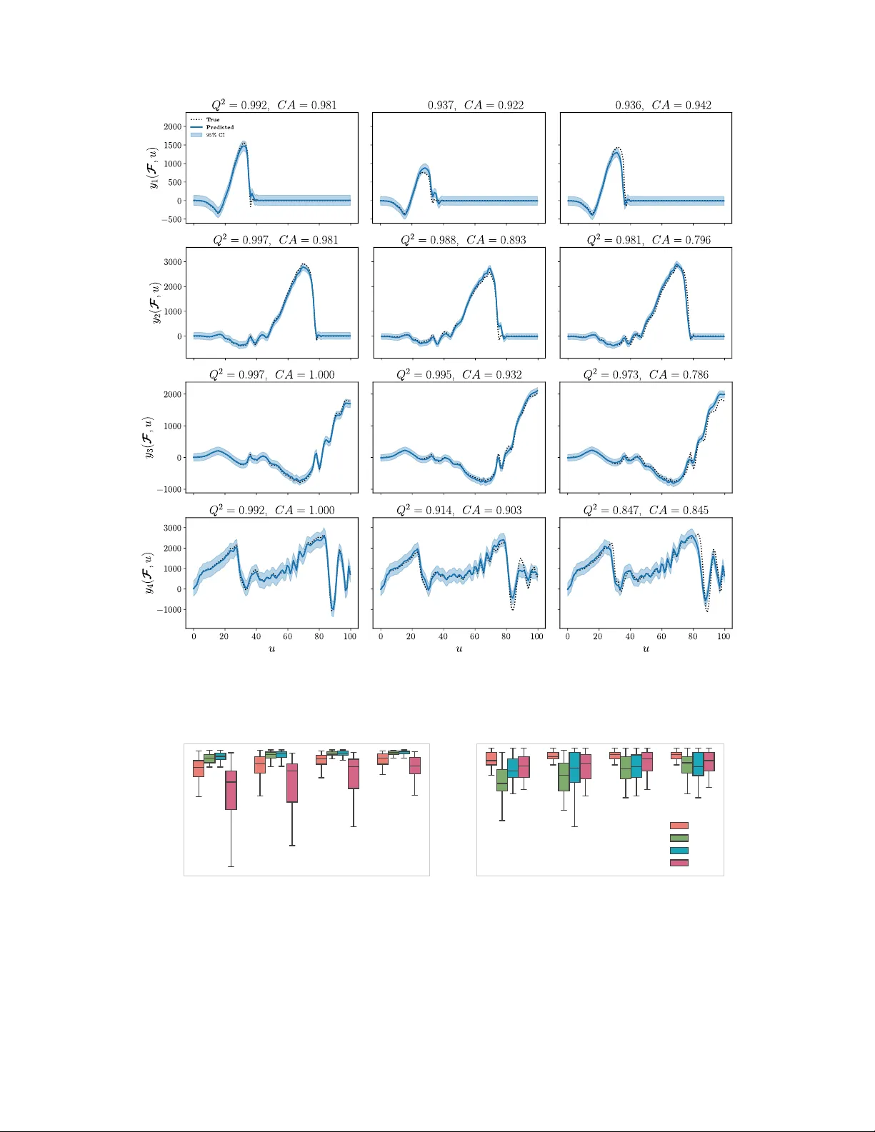
Scalable m ultitask Gaussian pro cesses for complex mec hanical systems with functional co v ariates Razak C. Sabi Gnink ou a , Andr ´ es F. L´ op ez-Lopera b,c , F ranc k Massa d , Ro dolphe Le Ric he e,f a Univ. Polyte chnique Hauts-de-F r anc e, INSA Hauts-de-F ranc e, CERAMA THS, V alenciennes, F-59313, F r anc e b Univ. de Montp el lier, IMAG, CNRS, Montp el lier, F-34090, F r anc e c Inria, LEMON, Montp el lier, F-34095, F r anc e d Univ. Polyte chnique Hauts-de-F r anc e, CNRS, UMR 8201 - LAMIH, INSA Hauts-de-F r anc e, V alenciennes, F-59313, F r anc e e CNRS, LIMOS, Clermont-F errand, F-63178, F r anc e f ´ Ec ole Nationale Sup´ erieur e des Mines de Saint- ´ Etienne, Saint- ´ Etienne, F-42023, F ranc e Abstract F unctional cov ariates arise in many scientiﬁc and engineering applications when mo del inputs take the form of time-dep endent or spatially distributed proﬁles, suc h as v arying b oundary conditions or changi ng material b e- ha viours. In addition, new practices in digital simulation require predictions accompanied b y conﬁdence in terv als. Mo dels based on Gaussian pro cesses (GPs) pro vide principled uncertain ty quantiﬁcation. Ho w ever, GPs capable of jointly handling functional cov ariates and multiple correlated functional tasks remain largely under-explored. In this work, w e extend the framework of GPs with functional cov ariates to m ultitask problems by introducing a fully separable kernel structure that captures dep endencies across tasks and functional inputs. By taking adv an tage of the Kronec ker structure of the co v ariance matrix, the mo del is made scalable. The prop osed mo del is v ali- dated on a syn thetic b enc hmark and applied to a realistic structure, a riv eted assem bly with functional descriptions of the material behaviour and response forces. The prop osed functional multitask GP signiﬁcantly improv es o ver single task GPs. F or the riveted assembly , it requires less than 100 samples to pro duce an accurate mean and conﬁdence interv al prediction. Despite its larger num be r of parameters, the multitask GP is computationally easier to learn than its single task p endan t. Keywor ds: computer exp erimen ts, surrogate mo deling, uncertaint y quan tiﬁcation, machine learning, functional data analysis 1. Introduction Gaussian pro cesses (GPs) provide a principled Ba yesian framew ork for regression, uncer- tain ty quantiﬁcation, and surrogate mo deling. By deﬁning probability distributions ov er func- tions, GPs oﬀer a ﬂexible wa y to learn complex nonlinear mappings while providing calibrated uncertain ty estimates, whic h is particularly adv an tageous when data are limited or expensive to acquire. As a result, GPs hav e b ecome a well-established approach for statistical mo deling across m ultiple disciplines, including mac hine learning [ 29 ], geostatistics [ 5 ], en vironmen tal mod- eling [ 35 ], computational mechanics [ 18 ], and robotics [ 8 ], where uncertain ty-a ware surrogate mo dels are essential for decision-making. In recen t y ears, the role of GP mo dels in computational mec hanics has signiﬁcantly expanded, driv en by the growing need for surrogate mo dels as an alternativ e to costly ﬁnite element or m ulti-physics simulations in application such as optimization, inv erse mo deling, reliability anal- ysis, and real-time monitoring [ 30 , 25 ]. Several studies ha v e demonstrated that GP-based surro- gates can accurately repro duce full-ﬁeld resp onses and structural quantities with only a limited Pr eprint submitte d to Computer Metho ds in Applie d Me chanics and Engineering F ebruary 25, 2026 n umber of high-ﬁdelity simulations, enabling eﬃcient uncertain ty quantiﬁcation and reliability assessmen t in large-scale mechanical systems [ 22 ]. As an example, a fully Bay esian calibration metho d has been introduced in [ 13 ] for computational mo dels with high-dimensional outputs. There, b oth ﬁeld observ ations and a limited num ber of simulator ev aluations are jointly mo d- eled through a GP emulator deﬁned on a lo w-dimensional basis. This dimensionality-reduction step makes Ba yesian inference and uncertaint y quantiﬁcation feasible for problems inv olving functional, spatial, or otherwise high-dimensional outputs. The GP paradigm to computer ex- p erimen ts has b een extended in [ 27 ] to handle b oth quan titativ e and qualitative factors, prop os- ing cov ariance structures that account for similarity across categorical lev els while preserving smo othness in con tinuous inputs. This line of works further broadened the applicabilit y of GP mo dels to complex (nonlinear, costly to ev aluate) design spaces that mix physical parame- ters, material types, and op erating conditions, making GPs an increasingly relev ant setting in computational mec hanics. Bey ond traditional regression tasks, GPs hav e also b een extended to op erator learning and in verse problems, enabling the identiﬁcation of physical input-output mappings gov erned by high-dimensional or even inﬁnite-dimensional function spaces [ 24 , 34 ]. These latter dev elopmen ts ha ve made GPs not only as blac k-b o x surrogates, but also ph ysics-a ware probabilistic mo dels capable of capturing structured dep endencies in mechanical and multi-ph ysics systems. Man y applications inv olv e functional inputs rather than scalar. Typical examples in mec han- ics include force–time loading paths, pressure pulses, temp erature-based material properties, or spatially distributed driving ﬁelds. In such cases, eac h experiment or simulation is character- ized by an en tire function describing the mec hanical driver applied to the system [ 20 ]. The outputs of interest, in contrast, usually corresp ond to multiv ariate time series, such as force or displacemen t resp onses measured at several structural lo cations. These resp onses often exhibit strong temp oral correlations and in terdep endencies across m ultiple tasks or sensors. T raditional GP mo dels typically assume ﬁnite-dimensional cov ariates and scalar outputs, whic h limits their direct applicability in the functional and m ultitask context. Consequently , surrogate mo del- ing b ecomes particularly c hallenging when the co v ariates must be treated as functions, while the system resp onses are correlated and coupled across tasks. This setting requires a coher- en t probabilistic framew ork capable of jointly mo deling functional similarities in the cov ariates, dep endencies in the outputs, and cross-task correlations. Sev eral approaches hav e b een prop osed to handle functional inputs. Classical methods from functional data analysis [ 28 ] are t ypically used to reduce inﬁnite-dimensional cov ariates by pro- jecting them onto a ﬁnite set of basis functions such as B-splines, F ourier series, or principal comp onen ts analysis (PCA), thereby enabling conv en tional regression in a ﬁnite-dimensional la- ten t space. More recen tly , GP models in [ 1 , 32 ] ha v e incorp orated functional similarities directly in to tailored kernel deﬁnitions, allowing the GPs to op erate ov er spaces of functions rather than ﬁnite-dimensional v ectors. How ever, these formulations are limited to single-output regression. Con versely , multitask GP (MTGP) models [ 3 ], along with their extensions based on pro cess con volutions [ 38 ] or graph-based correlations [ 4 ], are sp eciﬁcally designed to capture dep enden- cies across multiple output c hannels or tasks. T o the b est of our knowledge, only a limited n umber of w orks ha ve attempted to extend GP regression to settings inv olving functional co- v ariates and multiv ariate outputs. In particular, functional cov ariates can b e incorp orated into GP mo dels through semi-metric constructions deﬁned on inﬁnite-dimensional spaces [ 37 ]. In many mechanical systems, task-dep endent resp onse tra jectories are gov erned by shared ph ysical mechanisms and common sources of v ariabilit y , which induce strong inter-output cor- relations. Preserving and mo delling these correlations is therefore crucial to ensure coherent uncertain ty propagation and physically consistent predictions for resp onses indexed b y a con- tin uous v ariable. Ignoring such dependencies may lead to fragmented predictions and unreliable uncertain ty quantiﬁcation, esp ecially when resp onses are sparsely or unevenly observed across tasks. T o address the aforementioned limitations, we introduce an MTGP framew ork sp eciﬁcally tailored to mec hanical systems with functional cov ariates and multiple correlated tasks. The prop osed mo del relies on a fully separable kernel architecture that indep enden tly captures sim- ilarities across three dimensions: the task, the functional cov ariates and the scalar cov ariate 2 (e.g., the time). F or tensor-structured data, this construction induces a Kroneck er-pro duct de- comp osition of the cov ariance matrix, enabling exact yet scalable inference through structured tensor algebra. The resulting implementation, developed in PyTorch / GPyTorch [ 10 ], exploits GPU acceleration for eﬃcient computation of the marginal likelihoo d and p osterior predictions. The mo del is v alidated on b oth synthetic b enc hmarks and high-ﬁdelity mechanical simulations in volving multiple force–displacement resp onse curv es driv en b y nonlinear functional, loc al, force–displacemen t proﬁles. T o quantify the b eneﬁt of our in ter-task mo del, the MTGP is systematically compared against a single-task GP baseline. This work is structured as follows. Section 2 reviews the background of GP mo deling with functional cov ariates and summarizes the challenges asso ciated with functional data. Section 3 in tro duces our MTGP formulation for functional inputs and details the construction of the ker- nel, the parameter estimation, and the prediction. Section 4 presents tw o n umerical exp erimen ts. W e ﬁrst v alidate the prop osed MTGP with a synthetic example under ideal Gaussian settings, and then test the mo del on a real-world mechanical application, while assessing its predictive accuracy , its abilit y to capture cross-task dep endencies, and the computational p erformance. Section 5 summarizes the main results and gives an ov erview of relev ant future work. 2. Background 2.1. Gaussian pr o c esses with functional c ovariates In a functional regression setting, w e consider the problem of learning an unkno wn deter- ministic mapping y : F ( T , R ) d f → R , F 7→ y ( F ) , (1) where F ( T , R ) denotes the space of real-v alued functions deﬁned on a compact domain T ⊂ R . The functional cov ariate F = ( f 1 , . . . , f d f ) ∈ F ( T , R ) d f is a d f -dimensional vector of functions, and y ( F ) ∈ R denotes the associated scalar quantit y of interest. In a mec hanical con text, the functional co v ariate F ma y represen t a set of functional proﬁles, suc h as force-displacement resp onses, contact laws, or spatially v arying ﬁelds deﬁned ov er the domain T . The asso ciated output y ( F ) ma y then correspond to a resp onse extracted from the system b eha vior, for instance a characteristic force level, displacement or velocity ﬁelds, or a failure-related criterion. This functional regression setting serves as a generic starting p oint. More elab orate resp onse structures, inv olving multiple correlated outputs and ric her dependency patterns, will b e introduced in Section 3 . When mo deling computationally expensive computer co des, y is view ed as a black-box function for which only a small num b er of input ev aluations are feasible. T o address this c hallenge, an alternativ e probabilistic approac h is to mo del y as the realization of a sto c has- tic process { Y ( F ) } F ∈ F ( T , R ) d f , often assumed to be a GP . If Y is a GP , then, for an y ﬁnite collection F 1 , . . . , F n ∈ F ( T , R ) d f with F i = ( f i, 1 , . . . , f i,d f ), the associated random vector Y =  Y ( F 1 ) , . . . , Y ( F n )  ⊤ ∈ R n is multiv ariate Gaussian-distributed. In particular, under the standard zero-mean prior assumption, w e denote by con ven tion Y ∼ G P (0 , k ), where k is a k ernel function deﬁned as k : F ( T , R ) d f × F ( T , R ) d f − → R , ( F , F ′ ) 7− → k ( F , F ′ ) = Co v  Y ( F ) , Y ( F ′ )  . F or prediction purp oses, we are interested in computing the conditional distribution of Y giv en a training set D = { ( F i , y i ) } n i =1 , where F i denotes the co v ariate asso ciated to the i -th co de ev aluation y i ∈ R . Denote y =  y 1 , . . . , y n  ⊤ . According to the properties of Gaussian distributions, the predictiv e distribution of the response at a new input F ⋆ ∈ F ( T , R ) d f remains Gaussian: Y ( F ⋆ ) | y ∼ G P  m ( F ⋆ ) , v ( F ⋆ )  , 3 where the p osterior mean and p osterior v ariance are given b y m ( F ⋆ ) = k ( F ⋆ ) ⊤ K − 1 y , v ( F ⋆ ) = k ( F ⋆ , F ⋆ ) − k ( F ⋆ ) ⊤ K − 1 k ( F ⋆ ) . (2) with K ∈ R n × n the co v ariance matrix with en tries [ K ] 1 ≤ i,j ≤ n = k ( F i , F j ), and k ( F ⋆ ) ∈ R n the cross-co v ariance v ector with entries [ k ( F ⋆ )] 1 ≤ i ≤ n = k ( F ⋆ , F i ). The closed-form expressions in Eq. ( 2 ) are a k ey adv an tage of GP mo dels, oﬀering b oth predictiv e accuracy and uncertain t y quantiﬁcation for complex systems. While the p osterior mean m ( F ⋆ ) provides a p oin t prediction of the resp onse at F ⋆ , the posterior v ariance v ( F ⋆ ) quan tiﬁes the uncertaint y associated to the prediction. W e should remark that the deﬁnition of the posterior cov ariance co v( F ⋆ , F ′ ⋆ ) = k ( F ⋆ , F ′ ⋆ ) − k ( F ⋆ ) ⊤ K − 1 k ( F ′ ⋆ ) is often found in the literature. Ho w ever, in this paper we focus on the p osterior v ariance as this quantit y will later b e further developed using more eﬃcient Kroneck er-based op erations in the MTGP framew ork. 2.2. Construction of valid kernel A central c hallenge in GP models with functional cov ariates lies in designing kernels that are v alid on inﬁnite-dimensional input spaces. A common practice is to consider stationary k ernel obtained by comp osing a scalar-v alued function ψ : R + → R with a dissimilarity measure b et w een functions. This leads to kernels of the form k ( F , F ′ ) = ψ  ∥ F − F ′ ∥  , (3) where ∥ · ∥ denotes a dissimilarity measure on F ( T , R ) d f . This measure captures both amplitude and shap e v ariations across the domain, and the squared structure of ∥ F − F ′ ∥ makes the form ulation in Eq. ( 3 ) particularly well-suited for radial stationary kernels. It is imp ortan t to emphasize that an arbitrary choice of ψ , together with ∥ F − F ′ ∥ , do es not necessarily yield a p ositiv e semideﬁnite (psd) kernel. Radial kernels on general metric spaces are guaranteed to b e p ositiv e deﬁnite provided that ψ ( √ · ) is a completely monotone function [ 33 ]. Equiv alen tly , ψ admits the scale-mixture representation ψ ( t ) = Z ∞ 0 e − ω t 2 µ ( dω ) , t ≥ 0 , (4) where ω > 0 is a scale parameter controlling the smo othness of the elementary square exp onen tial (SE) kernel e − ω t 2 , and µ is a p ositive Borel measure on [0 , ∞ ) go verning the mixture of scales. This characterization pro vides the theoretical foundation for constructing isotropic kernels in functional settings. Building on these results, the theory of universal kernels shows that suc h radial constructions give rise to kernel families that are not only p ositiv e semideﬁnite but also dense in the space of contin uous functions [ 23 ]. W e m ust note that, while alternative dissimilarit y measures, such as the L ∞ -norm or Sob olev-type norms, may b e considered in theory , they do not guarantee p ositive semideﬁniteness when comp osed with an arbitrary function ψ . Ensuring this prop erty typically requires additional compatibility conditions, whic h are diﬃcult to v erify in practice [ 36 ]. F or these reasons, L 2 -based distances remain the most robust and widely used c hoice in the construction of k ernels for functional co v ariates. A particularly w ell-suited option is the w eighted L 2 -norm, deﬁned as ∥ F − F ′ ∥ 2 ℓ = d f X d =1 ∥ f d − f ′ d ∥ 2 L 2 ( T ) ℓ 2 d , (5) where ℓ = ( ℓ 1 , . . . , ℓ d f ) with ℓ d > 0 a length-scale parameter controlling the relative sensitivit y to v ariations in the d -th functional comp onent [ 1 ]. 4 Among the kernels that yield v alid constructions, a widely used class is the Mat´ ern family whic h is deﬁned, using the weigh ted L 2 -norm in ( 5 ), as k ( F , F ′ ) = σ 2 2 1 − ν Γ( ν )  √ 2 ν ∥ F − F ′ ∥ ℓ  ν K ν  √ 2 ν ∥ F − F ′ ∥ ℓ  , (6) where ν > 0 and σ 2 > 0 denote the smo othness and v ariance parameters (resp ectiv ely), and where Γ and K ν are the Gamma function and the mo diﬁed Bessel function of the second kind (resp.). Sp eciﬁc choices of the smoothness parameter ν lead to closed forms. F or instance, setting ν = 5 2 yields the Mat ´ ern- 5 2 k ernel, k ( F , F ′ ) = σ 2  1 + √ 5 ∥ F − F ′ ∥ ℓ + 5 3 ∥ F − F ′ ∥ 2 ℓ  exp  − √ 5 ∥ F − F ′ ∥ ℓ  , (7) and the choices ν = 1 2 and ν → ∞ recov er the exp onen tial and the squared-exp onential (Gaus- sian) kernels, resp ectively [ 11 ]. Hence, ν allows to control the regularity of the asso ciated GP: smaller v alues corresp ond to rougher sample paths, whereas larger v alues yield progressiv ely smo other tra jectories. In practical settings, functional co v ariates are only av ailable in discretized or ﬁnite- dimensional representations, which calls for suitable approximations of the L 2 -norm in Eq. ( 5 ) to be able to conduct kernel ev aluation and model training. Inspired by the techniques on functional data analysis, it is p ossible to approximate a functional input by a ﬁnite-dimensional subspace spanned b y an appropriate basis [ 28 ]. 2.3. Dimensionality r e duction for functional c ovariates Let { Υ d,r } p d r =1 b e a ﬁnite basis of L 2 ( T ), where T ⊂ R is a compact domain. W e can then pro ject each functional input f d , for d ∈ { 1 , . . . , d f } , on to this basis as Π( f d )( u ) = p d X r =1 β d,r Υ d,r ( u ) , (8) where the pro jection co eﬃcients β d = [ β d, 1 , . . . , β d,p d ] ⊤ are estimated by the minimization of the L 2 -norm of the residuals b et ween f d and Π( f d ). This procedure preserves the geometric structure of L 2 , while enabling ﬁnite-dimensional computations [ 28 , 1 ]. Using the pro jection in Eq. ( 8 ) for tw o functions f d and f ′ d , then the squared L 2 -distance can b e approximated by ∥ f d − f ′ d ∥ 2 L 2 ( T ) ≈ ( β d − β ′ d ) ⊤ Φ d ( β d − β ′ d ) , (9) where Φ d = R T Υ d ( u ) Υ ⊤ d ( u ) du with Υ d ( u ) =  Υ d, 1 ( u ) , . . . , Υ d,p d ( u )  ⊤ . Plugging this approxi- mated quan tity into in Eq. ( 5 ) gives the general approximation ∥ F − F ′ ∥ 2 ℓ ≈ d f X d =1 ( β d − β ′ d ) ⊤ Φ d ( β d − β ′ d ) ℓ 2 d . (10) Tw o useful simpliﬁcations follow from the structure of the Gram matrix Φ d . If the basis { Υ d,r } p d r =1 is orthonormal in L 2 ( T ), then Φ d = I and ∥ F − F ′ ∥ 2 ℓ ≈ d f X d =1 p d X r =1  β d,r − β ′ d,r  2 ℓ 2 d . (11) If the basis is orthogonal but not normalized, then Φ d = diag ( ϕ d, 1 , . . . , ϕ d,p d ), with ϕ d,r = R T Υ 2 d,r ( u ) du, and thus ∥ F − F ′ ∥ 2 ℓ ≈ d f X d =1 p d X r =1 ϕ d,r  β d,r − β ′ d,r  2 ℓ 2 d . (12) 5 A v ariety of basis function families are commonly used in functional data analysis, each tailored to sp eciﬁc structural prop erties of the signals. F or smo oth tra jectories, B-spline bases pro vide lo cal supp ort and ﬂexible control of smo othness [ 7 , 9 ]. F or p eriodic or nearly p erio dic b eha vior, F ourier bases are a natural c hoice [ 28 ]. T o represent lo calized and transient features, w av elet bases provide a m ultiresolution decomp osition that captures b oth time and scale infor- mation [ 6 , 21 ]. Beyond ﬁxed bases, empirical/data-driv en representations such as PCA reduces dimensionalit y by learning low-rank structure directly from the data [ 14 ]. V ariations in the application of PCA hav e b een considered in the literature where functional curves are ﬁrst rep- resen ted through a predeﬁned basis expansion after which PCA is p erformed to the resulting co eﬃcien t v ectors, as illustrated in the functional and wa v elet-based analysis in [ 31 ]. 3. Multitask Gaussian pro cesses with functional cov ariates According to our mechanical application described in Section 4.4 , and as in man y engineering and physical contexts, system resp onses are inﬂuenced not only by global op erating conditions, represen ted here b y functional co v ariates, but also v ary with respect to a ph ysical quan tit y . This additional cov ariate may corresp ond to prescrib ed displacemen t, time, frequency or a loading- cycle index (e.g., in fatigue analysis). In all such situations, the e v olution of the output along this ph ysical quantit y cannot b e fully captured by the functional cov ariates alone. F or this reason, w e consider a ph ysical cov ariate in addition to the functional ones. Although this cov ariate could b elong to a higher-dimensional space, w e will tak e it as one-dimensional in accordance with our the mec hanical application where it is a scalar displacemen t u ∈ R . How ev er, as the notation is k ept general, the extension to u ∈ R d u with d u > 1 is straightforw ard. Under this setting, w e introduce a m ultitask framework for mo deling multiple correlated tasks y s : F ( T , R ) d f × R → R for s ∈ { 1 , . . . , S } . The core of our formulation lies in a separable k ernel structure obtained through tensor pro ducts, that decomp oses input correlations into comp onen ts acting on the functional co v ariates, the scalar domain, and the task index. F or tensor-structured datasets, this construction induces a Kronec ker pro duct decomp osition of the full cov ariance matrix, which not only enables expressive mo deling but also ensures scalability of the inference and prediction pro cedures. 3.1. Mo deling with a sep ar able kernel structur e W e consider a m ultitask GP (MTGP) regression framew ork in whic h each output depends on a set of functional and scalar cov ariates. Let ( s, F , u ) ∈ S × F ( T , R ) d f × R , with F = ( f 1 , . . . , f d f ) and S = { 1 , . . . , S } , denote resp ectiv ely the index of the corresp onding task, the d f -dimensional functional co v ariate, and the scalar co v ariate, as deﬁned in Section 2 . The collection of all task-sp eciﬁc pro cesses { Y s } s ∈S is supp osed to deﬁne Y S = { Y s ( F , u ) } s ∈S ∼ G P (0 , k ), where Y S is GP-distributed v ector-v alued-function with k ernel k  ( s, F , u ) , ( s ′ , F ′ , u ′ )  = Co v  Y s ( F , u ) , Y s ′ ( F ′ , u ′ )  , (13) deﬁned on the extended input space S × F ( T , R ) d f × R . In this form ulation, the k ernel k join tly captures dep endencies across the task indexes ( s, s ′ ), the functional co v ariates ( F , F ′ ), and the scalar co v ariates ( u, u ′ ). A common mo deling assumption is that correlations induced by the input cov ariates and by the task structure can b e treated indep enden tly through a separable k ernel construction [ 3 ]. In our case, this assumption leads to k  ( s, F , u ) , ( s ′ , F ′ , u ′ )  = k S ( s, s ′ ) k f ,u  ( F , u ) , ( F ′ , u ′ )  , A similar assumption can also b e adopted to further separate the dep endence induced by the functional co v ariates from that associated with the scalar co v ariate, as commonly considered in kernel constructions in volving mixed v ariables [ 1 ]. Under this setting, the k ernel k can be written as k  ( s, F , u ) , ( s ′ , F ′ , u ′ )  = k S ( s, s ′ ) k f ( F , F ′ ) k u ( u, u ′ ) , (14) 6 where k S is a psd matrix whose en tries represent additional parameters of the model, k f en- co des correlations ov er the functional co v ariates, and k u captures correlations along the scalar co v ariate. In what follows, we assume that k f and k u are v alid kernels. Consequently , since the pro duct of psd kernels preserves the psd condition according to the Sch ur’s theorem, the kernel in Eq. ( 14 ) deﬁnes a v alid cov ariance function on S × F ( T , R ) d f × R [ 29 , 11 ]. By factorizing the k ernel into m ultiplicative comp onents asso ciated with the task index, the functional and scalar co v ariates, it captures in teraction eﬀects that cannot b e represented b y purely additive constructions [ 3 , 2 ]. The pro duct form further ensures that similarit y is preserved sim ultaneously across all dimensions, whic h reﬂects realistic settings where dep endencies arise join tly from multiple sources of v ariation. F rom a computational persp ective, the separable structure induces a Kroneck er pro duct form in the cov ariance matrix whenever the sampling design is tensor-structured, as we will discuss in Section 3.2 . This prop ert y , as shown in Section 3.3 , will enable eﬃcien t algorithms for matrix–vector pro ducts, log-determinan t ev aluations, and linear solves, thereby reducing memory and time complexit y compared to dense approac hes. Suc h scalability makes the resulting MTGP framew ork particularly w ell suited to large-scale datasets. 3.2. Hyp erp ar ameter estimation According to our mec hanical con text, observ ations are collected o ver a ﬁxed discretization grid { u j } n u j =1 ⊂ T , common to all functional cov ariates and tasks. Eac h functional replicate is indexed b y i ∈ { 1 , . . . , n f } and eac h task by s ∈ S , yielding resp onses Y s,i,j = Y s ( F i , u j ), for all triplets ( s, i, j ). Stac king all resp onses gives a single v ector Y ∈ R n with n = S n f n u . Under the GP assumption, Y follows a join t Gaussian distribution N ( 0 , K θ ), where the cov ariance entries are giv en by [ K θ ] ( s,i,j ) , ( s ′ ,i ′ ,j ′ ) = k S  s, s ′ ) k f  F i , F i ′ ) k u  u j , u j ′ ) , (15) with θ denoting the collection of hyperparameters inv olv ed in k f and k u , as well as the parame- ters deﬁning the p ositive semideﬁnite matrix k S . F or notational simplicity , we omit the explicit dep endence of these latter quantities on θ . The tensorized indexing associated to Eq. ( 15 ) implies that K θ can be written as a Kroneck er pro duct: K θ = K S ⊗ K f ⊗ K u , (16) with [ K S ] s,s ′ = k S ( s, s ′ ), [ K f ] i,i ′ = k f ( F i , F i ′ ), and [ K u ] j,j ′ = k u ( u j , u j ′ ). Such a decom- p osition greatly reduces the cost of matrix–vector pro ducts and log-determinant computations (see Section 3.3 ), and facilitates mo dular, interpretable kernel design [ 12 ]. Although Kroneck er pro ducts are not commutativ e, the order of the pro duct in Eq. ( 16 ) is essen tially without eﬀect in that it corresp onds to a reordering of the data through the ordering of the indices triplets ( s , F , u ). By considering the Mat´ ern kernel structure in Eq. ( 6 ) for k f and adopting an analogous k ernel construction for k u based on the Euclidean norm ∥ u − u ′ ∥ ℓ u , then we hav e the set of h yp erparameters θ =  K S , σ 2 , ℓ f , ℓ u  , (17) where K S ∈ R S × S enco des inter-task correlations, ℓ f = ( ℓ 1 , . . . , ℓ d f ) ∈ R d f + and ℓ u > 0 are the length-scale parameters of the functional and scalar k ernels (resp.), and σ 2 > 0 is a global v ariance parameter. W e note that separate v ariance parameters for the kernels k f and k u are not considered here, as this w ould lead to an iden tiﬁability issue: the ov erall v ariance of k would then b e given by the product σ 2 = σ 2 f σ 2 u . Although the Eq. ( 17 ) suggests that K S could b e estimated as a full symmetric psd matrix, this is rarely done in practice. A full-rank parametrization inv olves S ( S + 1) / 2 free parameters and often leads to p o or iden tiﬁability and numerical instabilities, esp ecially as S increases. An alternativ e in MTGP mo deling is to factorize K S via Cholesky decomp osition K S = L S L ⊤ S , L S ∈ R S × S , (18) whic h guarantees p ositiv e deﬁniteness (up to numerical tolerances), and can impro ve optimiza- tion stability . W e note that it is also possible to consider a low-rank factorization K S = C S C ⊤ S 7 with C S ∈ R R × S and R ≪ S , to reduce the amount of parameters that need to b e estimated. Ho wev er this later option is not further considered here as it do es not allo w further simpliﬁca- tions in the computation of the determinan t and inv ersion of K S , b oth quantities required in the lik eliho o d ev aluation (See Section 3.3 ). W e now turn to the estimation of θ , which is p erformed by minimizing the negativ e log- marginal lik eliho o d asso ciated with the MTGP mo del giv en by L ( θ ) = 1 2 log | K θ | + 1 2 y ⊤ K − 1 θ y + n 2 log(2 π ) , (19) with the observ ation v ector y = [ y 1 , . . . , y n ] ⊤ . This quan tity is typically minimized using gradien t-based optimizers such as L-BF GS or Adam [ 19 , 16 ]. F rom ( 19 ), we note that ev aluat- ing the L requires rep eated computations of K − 1 θ and log | K θ | . F or large multitask problems, these op erations become prohibitively exp ensiv e unless the Kronec k er structure of K θ is fully exploited. 3.3. Eﬃcient Kr one cker-b ase d infer enc e A key prop ert y of Kroneck er pro ducts is that the Cholesky decomp osition factorizes across tensor comp onents. Sp eciﬁcally , if K d = L d L ⊤ d , d ∈ {S , f , u } , then the global cov ariance matrix admits the Cholesky factorization K θ = L L ⊤ , L = L S ⊗ L f ⊗ L u ∈ R n × n , with n = S n f n u . This av oids computing the Cholesky decomp osition of the full matrix K θ , replacing it with the m uch cheaper decomp ositions of K S , K f , and K u . Using the Cholesky factorization, then Eq. ( 19 ) can b e rewritten as L ( θ ) = log | L | + 1 2 ∥ α ∥ 2 + n 2 log(2 π ) , (20) where L α = y is a linear system that can be solv ed by forward substitution. The key computa- tional challenge therefore lies in ev aluating b oth log | L | and α eﬃciently , with the latter b eing the most demanding op eration. F or the computation of log | L | (see App endix C.1 ), the separable structure yields the closed- form expression log | L | = ( n f n u ) S X i =1 log( L S ) ii + ( S n u ) n f X i =1 log( L f ) ii + ( S n f ) n u X i =1 log( L u ) ii . (21) This form ulation av oids computing | L | by ﬁrst forming the full Cholesky factor L ∈ R n × n , a step that can b e time-consuming. Instead, the computation reduces to the sum of the logarithms of the diagonal entries of the Cholesky factors L S , L f , and L u , calculations that can b e ac hieved more eﬃcien tly . W e now turn to the computation of α which is given by solving the linear system L α = y with L = L S ⊗ L f ⊗ L u . Using the inv ersion rule for Kronec ker pro ducts, w e obtain α = ( L − 1 S ⊗ L − 1 f ⊗ L − 1 u ) y . T o this end, the vector y ∈ R n is reshap ed in to the tensor Y ∈ R S × n f × n u , where the mo des corresp ond to tasks, functional replicates, and temp oral grid p oin ts. Using the identit y relating Kronec ker pro ducts and v ectorization (see App endix C.2 ), we obtain α = vec  Y × u L − 1 u × f L − 1 f × S L − 1 S  , (22) where × d denotes the mo de-wise multiplication along dimension d . These mo de-wise multipli- cations can b e achiev ed by solving the following linear systems: L u ( A (1) ) s,i, : = ( Y ) s,i, : , ∀ ( s, i ) , L f ( A (2) ) s, : ,j = ( A (1) ) s, : ,j , ∀ ( s, j ) , L S ( A (3) ) : ,i,j = ( A (2) ) : ,i,j , ∀ ( i, j ) , α = vec  A (3)  , (23) 8 where A (1) , A (2) , A (3) are in termediate tensors pro duced after eac h mo de-wise triangular solve. More precisely , the computation pro ceeds through a sequence of mo de-wise triangular solves. First, the lo w er triangular system L u ( A (1) ) s,i, : = ( Y ) s,i, : is solv ed along the scalar mo de for all ( s, i ), yielding the tensor A (1) . Similarly , the systems L f ( A (2) ) s, : ,j = ( A (1) ) s, : ,j and L S ( A (3) ) : ,i,j = ( A (2) ) : ,i,j are solved along the functional mo de for all ( s, j ) to ha v e A (2) and along the task mo de for all ( i, j ) to obtain A (3) . Note from Eq. ( 23 ) that the explicit computation of L − 1 is av oided, and that the ov erall complexit y is reduced to solving linear systems in volving Cholesky factors of smaller sizes. Consequen tly , this tensor-aw are computation reduces the naive cubic complexity O  ( S n f n u ) 3  to O  S n f n 2 u + S n u n 2 f + n f n u S 2  + O  S 3 + n 3 f + n 3 u  , where the ﬁrst term corresponds to the three mo de-wise triangular solves, and the second to the small Cholesky factorizations of K S , K f , and K u . Regarding memory usage, the requirement decreases from O  ( S n f n u ) 2  to O  S 2 + n 2 f + n 2 u  , since only the k ernel blo c ks and their Cholesky factors need to b e stored. 3.4. Posterior pr e diction Let y ∈ R n b e the observ ation vector, with n = S n f n u as deﬁned in Section 3.2 . F or a new test input ( F ⋆ , u ⋆ ) ∈ F ( T , R ) d f × R and a task index s ∈ { 1 , . . . , S } , the joint prior distribution of the training and test outputs is Gaussian:  y Y s ( F ⋆ , u ⋆ )  ∼ N 0 , K k ( s ) ⋆ k ( s ) ⊤ ⋆ k s ( F ⋆ , u ⋆ ) !! , where k ( s ) ⋆ =  k (( s, F ⋆ , u ⋆ ) , (1 , F 1 , u 1 )) , . . . , k  ( s, F ⋆ , u ⋆ ) , ( s, F n f , u n u )  ⊤ ∈ R n is the cross- co v ariance vector betw een the training set and the test p oint, K ∈ R n × n is the training co- v ariance matrix, and k s ( F ⋆ , u ⋆ ) = k (( s, F ⋆ , u ⋆ ) , ( s, F ⋆ , u ⋆ )) = σ 2 is the prior v ariance at this lo cation. F or notation simplicity , we inten tionally dropp ed the dep endency on the hyperparam- eters θ from the indices of the quantities implying the ev aluation of the k ernel k . By the Gaussian prop erties, the p osterior distribution of Y s ( F ⋆ , u ⋆ ) is also Gaussian: Y s ( F ⋆ , u ⋆ ) | y ∼ G P  m s ( F ⋆ , u ⋆ ) , v s ( F ⋆ , u ⋆ )  , with p osterior mean and v ariance are given by m s ( F ⋆ , u ⋆ ) = k ( s ) ⊤ ⋆ K − 1 y , v s ( F ⋆ , u ⋆ ) = σ 2 − k ( s ) ⊤ ⋆ K − 1 k ( s ) ⋆ . (24) The direct computation of m s ( F ⋆ , u ⋆ ) and v s ( F ⋆ , u ⋆ ) w ould normally require the explicit in version of the cov ariance matrix K , which is computationally prohibitive for large-scale multi- task settings. Instead, we can again exploit the Cholesky factorization K = LL ⊤ and reuse the v ector α already computed during likelihoo d optimization. The key eﬃciency gain arises from the Kronec ker-separable structure of the k ernel, which allo ws both k ( s ) ⋆ and L to b e decomp osed in to mo de-wise comp onen ts. F or the former term corresp onding to the cross-co v ariance vector, w e hav e k ( s ) ⋆ = [ k S ] s ⊗ k f ( F ⋆ ) ⊗ k u ( u ⋆ ) , with [ k S ] s =  k S ( s, 1) , . . . , k S ( s, S )  ⊤ , k f ( F ⋆ ) =  k f ( F ⋆ , F 1 ) , . . . , k f ( F ⋆ , F n f )  ⊤ , and k u ( u ⋆ ) =  k u ( u ⋆ , u 1 ) , . . . , k u ( u ⋆ , u n u )  ⊤ . As L − 1 = L − 1 S ⊗ L − 1 f ⊗ L − 1 u , combining b oth Kro- nec ker decomp ositions yields L − 1 k ( s ) ⋆ =  L − 1 S [ k S ] s  ⊗  L − 1 f k f ( F ⋆ )  ⊗  L − 1 u k u ( u ⋆ )  = ζ S ⊗ ζ f ⊗ ζ u , where the linear systems L S ζ S = [ k S ] s , L f ζ f = k f ( F ⋆ ) and L u ζ u = k u ( u ⋆ ) can b e solv ed by forw ard substitution. Using the ab ov e result and Eq. ( 22 ), the posterior mean is then given b y m s ( F ⋆ , u ⋆ ) = ( L − 1 k ( s ) ⋆ ) ⊤ α =  ζ ⊤ S ⊗ ζ ⊤ f ⊗ ζ ⊤ u  α , (25) 9 and the p osterior v ariance follows v s ( F ⋆ , u ⋆ ) = σ 2 − ( L − 1 k ( s ) ⋆ ) ⊤ L − 1 k ( s ) ⋆ = σ 2 − ( ζ ⊤ S ζ S )( ζ ⊤ f ζ f )( ζ ⊤ u ζ u ) . (26) where w e used the Kroneck er property ( ζ S ⊗ ζ f ⊗ ζ u ) ⊤ ( ζ S ⊗ ζ f ⊗ ζ u ) = ( ζ ⊤ S ζ S )( ζ ⊤ f ζ f )( ζ ⊤ u ζ u ). Note from Eq. ( 25 ) and Eq. ( 26 ) that both quan tities thus rely on mo de-wise triangular solv es and simple matrix–vector con tractions, and therefore, ensuring scalability while preserving n umerical stability . 4. Numerical exp erimen ts 4.1. Exp erimental setup Implemen tations are based on the GPyTorch library [ 10 ], and all exp erimen ts w ere conducted on a workstation equipp ed with an Intel(R) Core(TM) Ultra 7 155H pro cessor (16 physical cores, 22 logical pro cessors, up to 4.8 GHz) and 30 GB of RAM, running Ubuntu 24.04 L TS. The mo dels w ere implemented in Python 3.12.2 using PyT orch 2.5.1 and GPyT orch 1.14. The GPyT orch to olbox has b een adapted to compute the separable kernel structure introduced in Eq. ( 14 ), relying on the Kronec ker-based implementation describ ed in Section 3.3 . All the source co des, and the notebo ok required to partially repro duce the toy example in Section 4.3 , are publicly a v ailable at https://github.com/SABI- GNINKOU/F- MTGP . The predictive p erformance of the model is ev aluated on t wo datasets: (i) a syn thetic example designed to provide interpretable b eha vior and controlled v ariabilit y (Section 4.3 ), and (ii) a real dataset originating from a complex mechanical com ponent (Section 4.4 ). F or the synthetic example, a single functional enco ding strategy is adopted. Sp eciﬁcally , the functional inputs are pro jected onto a low-dimensional latent space using PCA, which pro vides a simple and in terpretable baseline in a con trolled setting. In contrast, the mechanical application in volv es functional inputs with more diverse proﬁles in terms of amplitude, smo othness, and frequency con tent. T o accoun t for this v ariabilit y , several functional dimensionality reduction strategies are considered and compared. These include PCA, functional basis expansions based on a Haar w av elet basis (lev el 4), B-splines, as well as hybrid approac hes in whic h PCA is applied to the corresp onding basis co eﬃcien ts, named here as “W a velet + PCA” and “B-spline + PCA”. A brief description of the previous enco ding strategies is giv en in App endix A . In all cases, the functional inputs are mapped to a latent space of ﬁxed dimension d pro j = 6, ensuring a fair comparison b etw een representations of comparable complexity . F or direct PCA, the six dimensions capture at least 99 . 9% of the total v ariance across the three functional comp onen ts. F or w av elet- and B-spline-based enco dings, the six most energetic co eﬃcien ts are retained. In the hybrid v ariants a whitened PCA with six laten t directions also explains approximately 99 . 9% of the total energy . Regardless of the c hosen functional enco ding, all mo dels are trained under the same op- timization protocol. Regarding the MTGP , k ernel op erations rely on Kronec k er-structured linear algebra, enabling eﬃcient ev aluation of the marginal lik eliho o d and its gradients. In all exp eriments, the hyperparameters are estimated by maximizing the marginal log-lik eliho o d using the Adam optimizer [ 16 ], with a learning rate η = 2 × 10 − 2 , momen tum parameters ( β 1 , β 2 ) = (0 . 98 , 0 . 999), and a w eight decay of 10 − 5 . Gradien t norms are clipp ed to a maximum v alue of 1 . 0 to impro ve numerical stabilit y during training [ 26 ], and an early-stopping criterion is applied when the log-lik eliho o d improv emen t remains b elo w 10 − 3 for 20 consecutiv e iterations. The maximum num b er of optimization iterations is se t to n max = 5 × 10 2 for the synthetic Ra yleigh-based example and n max = 2 × 10 4 for the mechanical application. The larger iter- ation budget allocated to the mechanical case reﬂects its higher dimensionalit y and increased complexit y , which require additional iterations to reach stable likelihoo d v alues. T raining the MTGP model for the mec hanical application is expected to b e more challenging than for the synthetic data, as the data–model consistency is not guaranteed in the presence of exp erimen tal noise, modeling errors, and complex physical in teractions. T o mitigate the risk of conv ergence to sub-optimal lo cal maxima of the marginal log-lik eliho od, a m ulti-start 10 optimization strategy is therefore employ ed for the mechanical case, using n restart = 10 ran- dom initializations. Before eac h restart, kernel hyperparameters are reinitialized within ranges adapted to the observ ed v ariabilit y of the mechanical resp onses sho wn in Figure 6 : ℓ f ∼ U ([0 . 5 , 20]) , ℓ u ∼ U ([0 . 005 , 0 . 1]) , σ 2 ∼ U ([0 . 5 , 2]) , σ 2 noise ∼ U ([10 − 3 , 10 − 1 ]) . Among all restarts, the model achieving the highest log-lik eliho od v alue is retained for subse- quen t predictions. 4.2. Performanc e criteria The predictive performance of the MTGP mo del is ev aluated on a set of test ev aluation p oin ts { ( F ⋆,i , u ⋆ ) } n test i =1 using t wo complementary criteria: the co eﬃcient of determination ( Q 2 ) and the co v erage accuracy (CA). F or eac h task s ∈ { 1 , . . . , S } , the MTGP predictive distribution at a test pair ( F ⋆,i , u ⋆ ) is characterized by its conditional p osterior mean m s ( F ⋆,i , u ⋆ ) and v ariance v s ( F ⋆,i , u ⋆ ), as given in Eq. ( 25 ) and Eq. ( 26 ). These predictions are compared to the corresp onding true simulator outputs y true s ( F ⋆,i , u ⋆ ). The determination co eﬃcien t is deﬁned as Q 2 s = 1 − P n test i =1 ( y true s ( F ⋆,i , u ⋆ ) − m s ( F ⋆,i , u ⋆ )) 2 P n test i =1 ( y true s ( F ⋆,i , u ⋆ ) − y s ) 2 , (27) where y s denotes the empirical mean of all test for task s . This quantit y measures the accuracy of the p oin t predictions relativ e to the in trinsic v ariability of the data. V alues of Q 2 s close to 1 indicate accurate predictions. The calibration of the predictive uncertaint y is quan tiﬁed through the cov erage accuracy of the predictiv e interv al I s ( F , u, δ ) = h m s ( F , u ) − δ p v s ( F , u ); m s ( F , u ) + δ p v s ( F , u ) i , deﬁned as CA s ( δ ) = 1 n test n test X i =1 1 { y true s ( F ⋆,i ,u ⋆,i ) ∈ I s ( F ⋆,i ,u ⋆ ,δ ) } . (28) This criterion estimates the prop ortion of test p oin ts lying inside the predictive in terv als. In our exp erimen ts, we set δ = 1 . 96, which corresp onds to a nominal 95% predictive interv al under Gaussian assumptions, so that a w ell-calibrated mo del should satisfy CA s (1 . 96) ≈ 0 . 95. 4.3. The R ayleigh-b ase d synthetic b enchmark 4.3.1. Dataset gener ation W e construct a synthetic dataset to ev aluate both the predictive accuracy and the scalabilit y of the MTGP mo del. T o guaran tee that the problem is w ell-p osed and a v oid complexities related to data-mo del mismatch [ 15 ], the dataset is constructed from samples of a baseline MTGP with kno wn parameters. It is then certain that the data can b e learned by the mo del. Inspired by the up coming mechanical application in Section 4.4 , we consider inputs F = ( f 1 , f 2 , f 3 ) where eac h f i follo ws a Rayleigh-shaped curve h ρ ( u ) = u ρ 2 exp  − u 2 2 ρ 2  , with u ∼ U ([0 , 1 . 5]) and ρ ∼ U ([0 . 05 , 1]). T o control the amplitude of the function, we use the rescaled form f i ( u ) ∼ α h ρ ( u ) max h ρ ( u ) , with α ∼ U ([2 , 4]). These functions are discretized ov er 150 p oin ts that is, each functional input F i = ( f i, 1 , f i, 2 , f i, 3 ) ∈ F ( T , R ) 3 consists of three full curves, represented after discretization as f i,d 7− →  f i,d ( u 1 ) , . . . , f i,d ( u 150 )  ∈ R 150 , d ∈ { 1 , 2 , 3 } . Thus, there are d f = 3 functional 11 0 . 0 0 . 5 1 . 0 1 . 5 u 0 1 2 3 4 f 1 ( u ) 0 . 0 0 . 5 1 . 0 1 . 5 u 0 1 2 3 4 f 2 ( u ) 0 . 0 0 . 5 1 . 0 1 . 5 u 0 1 2 3 4 f 3 ( u ) 0 . 0 0 . 5 1 . 0 1 . 5 u − 2 − 1 0 1 2 y 1 ( F , u ) 0 . 0 0 . 5 1 . 0 1 . 5 u − 3 − 2 − 1 0 1 y 2 ( F , u ) Figure 1: Rayleigh-based dataset. The panels sho w: (top) Samples of the three functional inputs F = ( f 1 , f 2 , f 3 ), randomly generated as Rayleigh-shaped functions h ρ , and (b ottom) the corresponding sampled outputs y 1 and y 2 generated by the baseline MTGP . c hannels and eac h input F i is a high-dimensional functional ob ject. F or the subsequen t steps the generated inputs are pro jected onto a 6-dimensional PCA basis. The baseline MTGP is equipp ed with the separable k ernel structure of Eq. ( 14 ) where k f is a Mat´ ern-5 / 2 kernel as deﬁned in Eq. ( 7 ) with ﬁxed length-scales ℓ f = (80 , 80 , 80). F or the scalar k ernel, we use the additive structure k u ( u, u ′ ) = k Mat ( u, u ′ ) + k Per ( u, u ′ ) where k Mat ( u, u ′ ) = 1 + √ 5 | u − u ′ | ℓ Mat + 5 | u − u ′ | 2 3 ℓ 2 Mat ! exp − √ 5 | u − u ′ | ℓ Mat ! , and k Per ( u, u ′ ) = exp  − 2 ℓ 2 Per sin 2  π | u − u ′ | p  , with parameters ℓ Mat = 1 . 5, ℓ Per = 0 . 5, p = 1. This choice com bines the smooth long-range b eha vior of a Mat ´ ern-5 / 2 kernel with the oscillatory structure induced b y a perio dic component. Suc h an additive kernel repro duces b oth transien t and quasi-p eriodic temp oral patterns, par- tially matc hing the dynamics observed in the real structural comp onent studied in Section 4.4 . The baseline MTGP is ev aluated at n f = 500 distinct functional inputs. Figure 1 sho ws the corresp onding outputs and input proﬁles generated in this synthetic exp erimen t. F or this example, the dataset accounts for t wo tasks, i.e., S = 2. The inter-task correlations are encoded through the matrix K S =  1 . 00 0 . 85 0 . 85 1 . 00  , which reﬂects a strong p ositiv e dep endence b etw een b oth tasks. The tw o tasks generated for each set of functional cov ariates are observed at n u = 100 p oin ts, resulting in a total num ber of n = S n f n u = 10 5 observ ations. The t wo outputs-sp eciﬁc y 1 ( F , u ) and y 2 ( F , u ) are jointly generated by the baseline MTGP . 4.3.2. Cr oss-validation test The predictiv e p erformance of the mo del is asse ssed using a leav e-one-out (LOO) cross- v alidation strategy . A t eac h fold, one en tire functional replicate is remov ed from the training set and used as the test input, while the mo del is retrained on the remaining n f − 1 replicates. T o ensure consistency across folds, all functional inputs, whether in the training or test set, are enco ded with the same discretization plus PCA pro cedure as describ ed ab o v e. Once the mo del is trained, the MTGP predictive mean and v ariance are ev aluated at all n u scalar p oints of the test curv e. This pro cedure is rep eated until each functional replicate has b een used once as 12 Scenario 45 Scenario 140 Scenario 429 Figure 2: LOO MTGP predictions for the test scenarios 45, 140, and 429 (display ed b y columns) of the Rayleigh- based dataset. These scenarios corresp ond to the “b est”, “av erage”, and “worst” predictive cases, respectively . The ground truth is sho wn in black, while predictions are shown in blue with 95% conﬁdence in terv als. s = 1 s = 2 0 . 970 0 . 975 0 . 980 0 . 985 0 . 990 0 . 995 1 . 000 Q 2 Figure 3: Q 2 boxplots computed o v er the 500 LOO cross-v alidation replicates used in the Ra yleigh- based dataset. Results are shown for e ac h output y s for s ∈ { 1 , 2 } . 25 100 175 250 n f 10 − 4 10 − 3 10 − 2 10 − 1 10 0 Execution time (s) Naive Pro duct T ensor Contraction Figure 4: Runtime for solving the linear system L α = y in the Ra yleigh-based dataset. The time is measured for diﬀerent num bers of functional dimensions n f . the test case, yielding an unbiased estimate of the predictiv e p erformance. Global accuracy is quan tiﬁed by aggregating the Q 2 scores o ver all LOO folds. Before analyzing the quantitativ e LOO results, we ﬁrst present in Figure 2 predictions for three scenarios to enable a visual comparison b et w een the true sim ulator resp onses and the MTGP posterior mean, along with the asso ciated 95% credible in terv als. Sp eciﬁcally , we displa y predictions for Scenarios 45, 140, and 429, representing the “b est”, an “av erage”, and the “w orst” cases in terms of the Q 2 v alues. W e observe that Scenarios 45 and 140 exhibit high predictive accuracy ( Q 2 ≥ 0 . 997) for both tasks, with a correct agreement b etw een predicted and true curv es and well-calibrated credible interv als. In contrast, although Scenario 429 yields low er Q 2 v alues ( Q 2 ≥ 0 . 988), b oth predictions and credible interv als remain accurate and successfully capture the output dynamics. Figure 3 rep orts now the distribution of the 500 LOO Q 2 scores for the t wo tasks. W e can note that the resulting distributions are highly concentrated, with median v alues close to one, indicating a stable and robust predictiv e b eha vior of the MTGP across all test replicates. Regarding the CA results, the model yielded v alues equal to one in all cases, indicating that the credible in terv als alwa ys co vered the target curves. W e hav e generally noticed that, as observ ed in Figure 2 , these in terv als closely follow the output dynamics while not b eing ov erly conserv ative. 13 Figure 5: Numerical mo del of the assembly . The panels show: (a) the ﬁnite element mesh and simulation conditions, and (b) the deformed shap e at the end of the simulation. 4.3.3. Computational b enchmark T o assess the computational b eneﬁt of exploiting Kronec k er algebra, we compare tw o im- plemen tations for applying a Kroneck er-structured linear op erator to a vector. More precisely , w e consider the computation of α . The ﬁrst approach, referred to as the naive implementation, explicitly forms the full Kronec k er product L = L S ⊗ L f ⊗ L u ∈ R n × n , and computes the matrix– v ector pro duct α using standard dense linear algebra routines. This strategy incurs a quadratic cost in n for eac h application of the op erator, as w ell as prohibitive memory requirements. The second approach corresponds to the prop osed tensorized implementation. In this case, the Kronec ker pro duct matrix L is never formed explicitly . Instead, the vector y is reshap ed in to a tensor Y ∈ R S × n f × n u , and the action of L − 1 is computed via a sequence of mo de-wise triangular solv es along the temp oral, functional, and task dimensions describ ed in Eq. ( 23 ). Both implementations are benchmark ed using the same factors ( L S , L f , L u ). W e measure the run time required to compute α for increasing functional dimensions n f ∈ { 25 , 100 , 175 , 250 } , a veraged ov er 50 rep etitions. Figure 4 compares the execution times of the naive Kroneck er implemen tation and the tensor con traction approac h as a function of the functional dimension n f . While b oth runtimes increase with n f , the naiv e implemen tation scales muc h more steeply , resulting in execution times one to t wo orders of magnitude larger than those of the tensorized form ulation ov er the considered range. This demonstrates the clear computational adv an tage of tensor contractions ov er explicit Kroneck er pro ducts, indep endently of cov ariance estimation or Cholesky factorization. 4.4. Applic ation to a rivete d me chanic al assembly The ob jective of this application is to study the dynamic response of a m ulti-material riv eted assem bly sub ject to uncertain ties in the constitutive b ehavior of the connectors. Because of the relativ ely recent adoption of self-piercing riveting, the material properties remain imp erfectly c haracterized. Using a limited set of high-ﬁdelit y n umerical simulations, we assess the ability of the prop osed MTGP to mo del the relationship b et w een the force–displacement resp onses of the connectors and that of the assembly , along with the abilit y of this mo del to quan tify the v ariability in the structural response. 4.4.1. Me chanic al assembly and numeric al mo del The mechanical structure consists of a ﬂat alumin um plate connected to an omega-shap ed plate in p oly amid 66 (P A66) b y tw o ro ws of nine self-piercing rivets. Such assemblies are commonly found in transp ortation vehicles, esp ecially in the automotive industry . The physical sim ulations of the structure are carried out with the ﬁnite elemen t mo del shown in Figure 5 a. All the degrees of freedom of the nodes lo cated on the right side of the P A66 omega-shap ed proﬁle are ﬁxed. A prescrib ed displacement is applied to the plate, rotated by − 20 ◦ around the x -axis. The deformed shap e of the assembly at the end of the numerical simulation is shown in Figure 5 b. F urther details on the ﬁnite element simulation of the assembly can b e found in [ 17 ]. 14 0 1 2 3 u 0 500 1000 1500 2000 2500 f 1 ( u ) 0 1 2 3 4 5 u 0 1000 2000 3000 f 2 ( u ) 0 1 2 3 u 0 1000 2000 3000 4000 f 3 ( u ) 0 20 40 60 80 100 u − 1000 0 1000 2000 y 1 ( F , u ) 0 20 40 60 80 100 u − 1000 0 1000 2000 y 3 ( F , u ) 0 20 40 60 80 100 u − 1000 0 1000 2000 3000 y 2 ( F , u ) 0 20 40 60 80 100 u − 2000 − 1000 0 1000 2000 3000 y 4 ( F , u ) Figure 6: F orce-displacement proﬁles of the riveted assembly . The panels sho w: (top) the force-displacement functional inputs F = ( f 1 , f 2 , f 3 ) associated with the connectors, and (bottom) the corresponding outputs y s , for s ∈ { 1 , . . . , 4 } , asso ciated with the mechanical assem bly , each corresponding to a distinct observ ation lo cation. The horizontal axis represents the prescrib ed displacemen t u expressed in millimeters ( mm ), while the vertical axis represents the corresp onding force y s expressed in Newtons ( N ). 4.4.2. Datab ase description The connectors are mec hanically c haracterized b y three functional data F = ( f 1 ( u ) , f 2 ( u ) , f 3 ( u )) (see Figure 6 , top panel), corresp onding to the force–displacement resp onses under pure tension, combined tension–shear, and pure shear loadings, resp ectiv ely . The diﬀer- en t samples reﬂect material-related uncertainties associated with elastic, plastic and damage b eha viors, and constitute the functional cov ariates used as inputs to the MTGP mo del. When sampling the inputs, the same triplet F is assigned to all connectors of the assem bly . In other w ords, every connector within the structure receiv es the sam e functional inputs ( f 1 , f 2 , f 3 ) as it is assumed that it is made of the same material. Seven t y-eigh t samples are employ ed to explore the design space of these functional inputs. F or each sampled triplet F , a full nonlinear explicit ﬁnite element simulation is run with the Abaqus soft ware to extract the corresp onding force–displacemen t resp onses of the assembly . Each ﬁnite element simulation requires sev eral hours of computation, which strongly motiv ates the dev elopmen t of surrogate mo dels capable of deliv ering predictions of the connector and assembly resp onses under functional inputs. F our output functional resp onses ( y 1 ( F , u ) , y 2 ( F , u ) , y 3 ( F , u ) , y 4 ( F , u )) (Figure 6 , b ottom panel) are considered, corresp onding to the force-displacemen t resp onses of the left connectors in the ﬁrst three rows and to the global structural resp onse. In a compact form, the resulting dataset is expressed as the functional mapping F = ( f 1 ( u ) , f 2 ( u ) , f 3 ( u )) 7→ ( y 1 ( F , u ) , y 2 ( F , u ) , y 3 ( F , u ) , y 4 ( F , u )) . In the MTGP mo del, the similarity b et w een functional inputs is mo deled through the func- tional kernel k f , implemented as a Mat´ ern 5 / 2 co v ariance acting on the laten t functional rep- resen tations. The corresp onding length-scales are initialized to (20 , 20 , 20), enforcing a smo oth prior across the functional dimensions b efore b eing optimized during training. Displacements are mo deled using a scalar kernel k u , deﬁned as a Mat´ ern 5 / 2 cov ariance function. The initial 15 s = 1 s = 2 s = 3 s = 4 0 . 4 0 . 6 0 . 8 1 . 0 Q 2 s = 1 s = 2 s = 3 s = 4 0 . 4 0 . 6 0 . 8 1 . 0 CA PCA W av elet B-spline W av elet + PCA B-spline + PCA Figure 7: Predictive accuracy ( Q 2 , left) and uncertaint y quan tiﬁcation (CA with δ = 1 . 96, right) obtained with n f = 78 training cases and n test = 50 test cases, across the four tasks ( s = 1 , . . . , 4), using diﬀerent functional dimensionality reduction metho ds. length-scale is set to 10 mm and constrained to the interv al [1 , 50] mm to ensure n umerical stabilit y and physically meaningful spatial v ariabilit y . These choices are consistent with the displacemen t op erating range observed in the output proﬁles shown in Figure 6 (b ottom panel). 4.5. R esults and discussion 4.5.1. Imp act of functional dimensionality r e duction on pr e dictive p erformanc e The purp ose of this exp eriment is to assess the inﬂuence of the functional dimensionalit y reduction strategy on the predictive p erformance of the MTGP mo del. Figure 7 rep orts results obtained with n f = 78 training functions and n test = 50 test functions, for the four tasks ( s ∈ { 1 , 2 , 3 , 4 } ), comparing PCA, wa v elet, B-spline, and hybrid wa v elet+PCA and B-spline+PCA enco dings. F rom a predictiv e accuracy p erspective, it can b e observed that the direct PCA- based enco ding yields the highest p erformance across all tasks. This trend is particularly visible for the most challenging outputs, where PCA exhibits higher median accuracy together with reduced disp ersion, suggesting a more stable predictive behavior. Moreov er, the PCA predictive in terv als, as measured by the CA, remain close to the nominal cov erage lev el (ab out 0.95 for δ = 1 . 96), indicating an uncertaint y quantiﬁcation that matches well the model assumptions. Among the pro jection-based approaches, the B-spline enco dings ac hiev e results that are close to those obtained by the PCA. With the B-splice, the p erformance remains relatively stable ac ross tasks, b oth in terms of predictiv e and uncertain ty accuracy , whic h suggests that B-splines provide an eﬀective low-dimensional representation of the functional inputs. By contrast, the wa v elet- based represen tation leads to lo wer predictive accuracy and increased v ariabilit y , esp ecially for outputs y 1 and y 4 , whic h are characterized by more complex resp onse patterns. Applying PCA to the wa velet co eﬃcients partially mitigates these limitations: the W av elet+PCA strategy impro ves both the median accuracy and the stabilit y of the predictions compared to ra w wa velet features. How ev er, its p erformance remains b elo w that of direct PCA and B-spline enco dings. Similarly , the B-spline+PCA v ariant induces only limited c hanges relativ e to the original B- spline representation, indicating that the B-spline coeﬃcients are already w eakly correlated and suﬃcien tly structured, so that additional linear compression provides little impro v ement. Ov erall, these results indicate that direct PCA-based functional encoding oﬀers a fa vorable compromise b et ween predictive accuracy , robustness, and uncertaint y quantiﬁcation across the four tasks. F or this reason, PCA is retained as the functional dimensionality reduction metho d in all subsequen t exp erimen ts. T o further illustrate these results, w e now examine the MTGP predictions ov er test scenarios. In Figure 8 , prediction examples are rep orted for three selected test scenarios (23, 40, and 29) whic h corresp ond, resp ectiv ely , to the “b est”, “a verage”, and “w orst” predictive cases according to the Q 2 criterion. The results are sho wn for all four tasks. F rom the ﬁgure, one can observe that the ﬁrst three resp onses ( y s , s = 1 , 2 , 3) are generally reconstructed with go od accuracy , whereas the fourth task ( s = 4) displa ys a comparativ ely lo w er lev el of agreemen t. This b eha vior is consisten t with the trends previously seen in Figure 7 . This diﬀerence is not unexpected, since the output y 4 corresp onds to a more global structural resp onse that aggregates complex lo cal 16 Scenario 23 Scenario 40 Scenario 29 Figure 8: MTGP predictions for scenarios test 23, 40, and 29 (displa yed by columns) of the riveted assembly . These scenarios represent the b est, the av erage, and the w orst predictive cases, respectively , in terms of the Q 2 criterion. The ground truth is the black dotted line, while the predictions are plotted in blue with the 95% conﬁdence interv als . 26.0 40.0 52.0 78.0 n f 0 . 6 0 . 7 0 . 8 0 . 9 1 . 0 Q 2 26.0 40.0 52.0 78.0 n f 0 . 4 0 . 5 0 . 6 0 . 7 0 . 8 0 . 9 1 . 0 CA s = 1 s = 2 s = 3 s = 4 Figure 9: Inﬂuence of the training set size on predictive accuracy ( Q 2 , left) and uncertaint y calibration (CA, right) across the four tasks ( s = 1 , . . . , 4) for the riveted assembly test case. eﬀects and in volv es stronger nonlinearities. Despite this increased level of diﬃcult y , the MTGP remains able to capture the main temp oral evolution of the global y 4 in a generalization regime. F or completeness, additional prediction results obtained with alternative functional pro jec- 17 tion metho ds are provided in App endix B . 4.5.2. Inﬂuenc e of the tr aining set size on pr e diction and unc ertainty c alibr ation W e now inv estigate how the size of the training set inﬂuences b oth the predictive accuracy and the uncertain ty quantiﬁcation of the MTGP mo del. T o this end, the num b er of training functions is gradually increased ( n f ∈ { 26 , 40 , 52 , 78 } ), with eac h dataset constructed in a nested manner within the larger ones. The corresp onding results are reported in Figure 9 . As could b e exp ected, increasing the training set size leads to a improv ement in predictiv e p erformance across all tasks. This evolution is reﬂected by higher Q 2 v alues together with cov erage accuracy progressiv ely approaching the reference level, indicating a gradual improv emen t in uncertaint y calibration as more training information becomes av ailable. A closer insp ection reveals that, for tasks y 2 and y 3 , a high predictive accuracy is already achiev ed with relatively small training sets, with Q 2 v alues close to one as so on as n f exceeds 40. How ev er, for these tasks, the corresp onding cov erage accuracy remain b elo w the levels obtained for n f = 78. Although the predictiv e mean is accurately captured at an early stage, the asso ciated predictive uncertaint y tends to be underestimated, leading to o v erly narro w prediction in terv als. Such underestimation of the uncertain ty is related to the estimated inter-task correlation structure, as illustrated by the task correlation matrix K S (Figure 13 ), which sho ws strong dep endencies betw een tasks y 2 and y 3 . There, information sharing across tasks supports accurate mean prediction even with limited data, while the estimation of task-sp eciﬁc uncertaint y remains more sensitive to the size of the training set. As the num b er of training functions increases, this eﬀect progressively diminishes, resulting in impro ved uncertaint y calibration across all tasks. 4.5.3. Assessment of pr e dicte d c alibr ation envelop es Bey ond p oin twise accuracy , a reliable surrogate must provide uncertaint y estimates that are consisten t with the v ariabilit y of the true system. T o assess this property , we compare the MTGP predictiv e b eha vior with the empirical dispersion of the test responses through a calibration en velope analysis. F or each task s , the collection of true simulator outputs { y true s ( F ⋆,i , u ⋆ ) } n test i =1 asso ciated with all test functional inputs is used to construct an empirical 95% env elop e deﬁned b y CI true s =  q 2 . 5%  y true s ( F ⋆,i , u ⋆ )  , q 97 . 5%  y true s ( F ⋆,i , u ⋆ )  , where q 2 . 5% and q 97 . 5% denote the empirical 2 . 5th and 97 . 5th p ercentiles, resp ectiv ely . This en velope represents the v ariabilit y of the mechanical resp onse induced by the diversit y of material conditions, and serv es as a reference for assessing the consistency of the surrogate predictions. A t the same ev aluation p oin ts, the MTGP predictive distribution is c haracterized by its con- ditional p osterior mean and v ariance, denoted b y m s ( F ⋆,i , u ⋆ ) and v s ( F ⋆,i , u ⋆ ), resp ectiv ely , as deﬁned in Eq. ( 25 ) and Eq. ( 26 ). Two complementary asp ects of uncertain ty are then exam- ined. First, we quantify the v ariability of the predicted resp onse across test functional inputs through the disp ersion of the MTGP predictive means { m s ( F ⋆,i , u ⋆ ) } n test i =1 . This v ariabilit y is summarized b y the empirical 95% env elope CI m s = [ q 2 . 5% ( m s ( F ⋆,i , u ⋆ )) , q 97 . 5% ( m s ( F ⋆,i , u ⋆ ))] . Second, we assess the lo cal epistemic uncertaint y con v eyed b y the predictive v ariance v s ( F ⋆,i , u ⋆ ). F or each test input, a point wise uncertaint y b ound is deﬁned as m s ( F ⋆,i , u ⋆ ) ± 1 . 96 p v s ( F ⋆,i , u ⋆ ). Aggregating these b ounds o ver all test inputs yields the env elop e CI v s =  q 2 . 5%  m s ( F ⋆,i , u ⋆ ) − 1 . 96 q v s ( F ⋆,i , u ⋆ )  , q 97 . 5%  m s ( F ⋆,i , u ⋆ ) + 1 . 96 q v s ( F ⋆,i , u ⋆ )  . Ov erlaying the three env elopes, CI true s , CI m s and CI v s , provides a visual diagnostic of uncer- tain ty calibration where CI true s serv es as the reference for the intrinsic v ariability of the mechan- ical resp onse o ver the set of test functional inputs. This is done in Figure 10 . CI true s highligh ts regions of increased disp ersion, that o ccur in particular in transient regimes and high-amplitude resp onse zones. The MTGP predictive mean (solid blue curve) closely follows the empirical mean of the true sim ulator resp onses (black dotted curv e), including in regions characterized 18 0 20 40 60 80 100 u 0 1000 2000 3000 y 2 ( F , u ) 0 20 40 60 80 100 u − 1000 0 1000 2000 3000 y 4 ( F , u ) Figure 10: Calibration env elopes for the four MTGP tasks. The orange band sho ws the empirical 95% en velope of the true simulator resp onses CI true s , the translucent blue region is the predictiv e env elop e from the dispersion of GP mean predictions, CI m s and the dashed grey curves denote the 95% p osterior credible interv al, CI v s . The solid blue line is the MTGP predictive mean, and the black dotted line represents the empirical mean of the true responses. b y rapid temporal v ariations. This agreement suggests that the dominant temp oral structure of eac h output is well captured by the surrogate mo del. The disp ersion of the MTGP predictive means across test functional inputs, summarized b y the predictiv e env elope CI m s (blue shaded area) is similar in most regions to that of the empirical env elop e, indicating that the MTGP repro duces, to a large extent, the v ariability induced b y changes in the functional inputs. Still minor diﬀerences b et ween CI m s and CI true s can b e found at sharp changes in trend. On the other hand, the uncertaint y bands derived from the predictiv e v ariance, CI v s (dashed grey curv es), provide insight in to the epistemic uncertaint y of the surrogate mo del. These bands are wider than the empirical env elope, suc h conserv atism b eing more pronounced, relatively , when resp onses are near constant. Generally how ev er, CI v s remains compatible with the scale of the empirical en v elop e. The larger width of CI v s with resp ect to CI true s and CI m s is b ecause the epistemic uncertainties on the inputs are taken into accoun t twice, once through the v ariance v s , and another time through the quantiles on the inputs. Ov erall, these exp erimen ts show that the MTGP p erforms well b oth in terms of predictiv e accuracy and uncertain ty quan tiﬁcation, thereby supp orting its use as a reliable surrogate mo del for the considered mec hanical application. 4.5.4. MTGP versus single-task GPs In order to quantify the beneﬁt of explicitly modeling in ter-task dep endencies, this section compares the prop osed MTGP with functional inputs to its single-task GP counterpart, whic h assumes statistical indep endence among the tasks. In the single-task setting, each task s ∈ { 1 , . . . , S } is mo deled indep endently according to Y s ( F , u ) ∼ G P  0 , k f ( F , F ′ ) k u ( u, u ′ )  , where k f and k u capture correlations o v er the functional and temporal domains, respectively . The asso ciated hyperparameter vector is θ =  σ 2 , ℓ f , ℓ u  , with σ 2 denoting the global v ariance parameter, and ℓ f and ℓ u the length-scale parameters of k f and k u . The MTGP extends this form ulation by introducing an explicit task-co v ariance matrix K S , endow ed with its own parameters, so that the only structural diﬀerence b et w een the tw o mo dels lies in the explicit 19 s = 1 s = 2 s = 3 s = 4 0 . 7 0 . 8 0 . 9 1 . 0 Q 2 s = 1 s = 2 s = 3 s = 4 0 . 2 0 . 4 0 . 6 0 . 8 1 . 0 CA MTGP GP Figure 11: Comparison of the prediction accuracy and uncertaint y calibration between MTGP and single-task GPs for a training size of n f = 78. The left panel rep orts the Q 2 distributions across the four output tasks, while the righ t panel shows the C A cov erage accuracy . Figure 12: Comparison b etw een MTGP and single-task GP predictions for scenarios 23 (b est), 40 (av erage), and 29 (worst). Results are sho wn for the tasks (top) s = 3 and (bottom) s = 4, corresp onding resp ectiv ely to the tasks for whic h the MTGP yields the highest and low est Q 2 v alues. mo deling of cross-task correlations. F or this comparison, b oth the single-task GP and the MTGP mo dels are trained under iden- tical conditions, using the same m ulti-start optimization strategy and initialization settings, and with a ﬁxed training size of n f = 78, ensuring a fair and consistent ev aluation. W e then compare the predictiv e accuracy and the uncertaint y calibration obtained with the t wo approaches. As shown in Figure 11 , the MTGP consistently ac hieves higher Q 2 v alues than the indep en- den t GP across tasks, while maintaining predictive in terv als well calibrated around the nominal 95% lev el. These results indicate that explicitly mo deling cross-task co v ariance improv es predic- tiv e accuracy without degrading uncertaint y quantiﬁcation. By drawing up on statistical links across outputs, the MTGP provides a more coheren t and eﬃcien t representation of the multitask system. The example predictions reported in Figure 12 illustrate the b eha vior of the GP and the MTGP for outputs s = 3 and s = 4 under the scenarios 23 (b est case), 40 (av erage case), and 29 (w orst case). The MTGP model pro vides a more robust reconstruction of the temp oral dynamics in all the cases. Its predictive mean trac ks the true tra jectories more accurately , including in regions exhibiting rapid v ariations or oscillations (most notably for the scenario 29 for s = 4), whereas the GP shows visible deviations around peaks and regime changes. A key diﬀerence lies in the uncertaint y quantiﬁcation. The MTGP credible interv als (in blue) are wider than those of the GP , y et they remain regular and consistent with the intrinsic v ariability of the simulator. 20 s = 1 s = 2 s = 3 s = 4 s = 4 s = 3 s = 2 s = 1 − 1 . 0 − 0 . 8 − 0 . 6 − 0 . 4 − 0 . 2 0 . 0 0 . 2 0 . 4 0 . 6 0 . 8 1 . 0 Figure 13: Estimated inter-task correlation matrix K S for the four tasks in volv ed in the riveted assembly application. Red (resp ectively blue) ellipses indicate p ositive (resp. negative) correlations, with orientation encoding the sign and eccentricit y reﬂecting the magnitude. 26 40 52 78 n f 0 . 6 0 . 8 1 . 0 Q 2 MTGP GP 26 40 52 78 n f 0 . 25 0 . 50 0 . 75 1 . 00 CA Figure 14: Ev olution of predictive accuracy and uncertain ty calibration with increasing training size ( n f ∈ { 26 , 40 , 52 , 78 } ) for MTGP and GP models. This controlled width reﬂects the fact that the MTGP accoun ts for b oth lo cal uncertaint y and in ter–task correlations, thereb y preven ting the artiﬁcial underestimation of predictive v ariance. By contrast, the GP exhibits a more unstable behavior. In some regions, its credible in terv als are extremely narro w or ev en barely visible, indicating a substan tial underestimation of uncertain t y . Ov erall, they remain en tirely con tained within the MTGP in terv als, revealing the absence of an y mec hanism to propagate information across correlated outputs. Such ov erly optimistic interv als do not reﬂect the true v ariability of the resp onses and lead to unreliable uncertain ty estimates. Ov erall, these results demonstrate that explicitly mo delling inter–task correlations enhances b oth the ﬁdelit y of the predictions and the credibility of the asso ciated uncertain t y , whereas indep enden t mo delling fails to guarantee these prop erties. T o quantify the dep endencies seen in the data, Figure 13 presen ts the task-correlation matrix K S estimated after training the MTGP . Substan tial correlations are observed most notably a pronounced negative correlation b et w een tasks s = 2 and s = 3. This conﬁrms the intuition that the mec hanical resp onses at neighboring rivets are more correlated, th us justifying the use of a m ultitask formulation to jointly learn the rivets force-displacement relationship. T o further compare the dep endencies of b oth single and multi-task GPs on data av ailability , w e analyze how their predictive p erformances evolv e as the num ber of training functions increases ( n f ∈ { 26 , 40 , 52 , 78 } ). Figure 14 summarizes this evolution for both Q 2 and CA metrics. Each b o xplot represen ts the distribution of these metrics a v eraged o v er the four tasks for b oth mo dels. The results show that, as the training set grows, b oth mo dels impro ve in terms of accuracy and uncertain ty calibration. How ev er, the MTGP , whic h is marginally b etter than the GP in terms of Q 2 when n f = 26, leads to faster impro vemen ts and rapidly achiev es higher Q 2 scores and b etter-calibrated cov erage rates, demonstrating its ability to exploit shared information across tasks and to generalize more eﬃcien tly under data-limited conditions. 21 Mo del T raining Time (s) [10 2 ] Prediction Time (s) [10 − 2 ] GP s = 1 6 . 38 4.0 GP s = 2 11 . 40 3.9 GP s = 3 7 . 20 4.0 GP s = 4 21 . 50 4.3 MTGP 1 . 66 50.3 T able 1: Average training and prediction times p er test scenario for the single-task GP and the MTGP mo dels. 0 2500 5000 7500 10000 12500 15000 17500 20000 Iteration 10 1 10 2 10 3 10 4 10 5 L ( θ ) MTGP GP s = 1 GP s = 2 GP s = 3 GP s = 4 Figure 15: Optimization conv ergence comparison b etw een indep endently trained single-task GP models and the MTGP . The rep orted curves corresp ond to the av erage negative log-marginal likelihood L ( θ ) computed ov er ﬁve runs, plotted as a function of the num ber of training iterations. F rom a computational standp oin t, w e observe a reduction in training time un til optimization con vergence as rep orted in T able 1 . While the CPU times for the four independently trained GPs range from approximately 10 min utes to more than 30 min utes, the one for MTGP is ab out 3 minutes on av erage. All rep orted times corresp ond to the mean ov er ﬁve indep enden t runs with diﬀerent random initialization, with v ariations of approximately 1% in b oth the ﬁnal training time and the attained log-marginal likelihoo d v alues, indicating reliable rep eatabilit y of the optimization pro cedure. This gain in computing eﬃciency was not anticipated as the MTGP mo del has more parameters to learn than the GP . Suc h empirical gain is explained b y the conv ergence behavior sho wn in Figure 15 , where w e observe that the MTGP rapidly decreases the negative log-marginal likelihoo d and reaches a near-stationary regime after appro ximately 3 × 10 3 iterations. In contrast, the single-task GP mo dels exhibit a slow er deca y , with some tasks requiring more than 10 4 iterations to reac h comparable log-likelihoo d v alues. This b ehavior can b e in terpreted in ligh t of the theoretical prop erties of multitask learning curv es. In the presence of non-zero inter-task correlations, the prediction error on a given task depends not only on its own sample size but also on the n umber of observ ations av ailable for correlated tasks. When tasks are mo derately to strongly correlated, an initial collective learning phase o ccurs, during which the error decreases rapidly due to shared statistical structure. This translates into a more fa v orable marginal likelihoo d landscap e for the joint mo del, yielding faster practical con vergence. This is indeed the case in our study where tasks y 2 , y 3 , and y 4 exhibit non-negligible positive and negative correlations. W e can then conclude that the acceleration observed here is due to the explicit coupling of tasks through the learned inter-task co v ariance matrix K S . Its oﬀ-diagonal entries quan tify statistical transfer, and its spectral structure determines the dominant shared mo des across tasks. Joint hyperparameter estimation concentrates learning in a low er-dimensional shared subspace, whereas single-task GPs repeatedly estimate similar structural patterns separately , leading to redundan t optimization eﬀort. The situation diﬀers at the prediction stage. As rep orted in T able 1 , the av erage prediction time of the single-task GPs is 0 . 04 s, whereas the MTGP requires 0 . 50 s to join tly predict the four outputs. F or a single-tas k GP , prediction requires solving a linear system asso ciated with n f n u = 8112 degrees of freedom for each task indep enden tly . In con trast, the MTGP jointly mo dels the S = 4 correlated tasks, leading to a global eﬀective system size of S n f n u = 32448. This fourfold 22 increase in eﬀectiv e dimension directly explains the higher computational cost at prediction time. Although the Kroneck er factorization ensures that computations remain tractable and memory- eﬃcien t, the coherent coupling of all four outputs within a uniﬁed m ultitask framew ork naturally en tails a higher computational burden than fully decoupled single-task mo dels. More precisely , prediction still requires coupled linear solves and structured matrix–vector op erations inv olving all tasks sim ultaneously . This in terpretation was conﬁrmed b y the CPU proﬁling results. F or a single MTGP prediction, more than 50% of the computation time is sp en t in dense matrix m ultiplications, and approximately 44% in linear system solv es, while kernel ev aluation itself represen ts a negligible fraction of the total cost. 5. Conclusions and future work This work in tro duces a scalable multitask Gaussian pro cess (MTGP) designed for systems whose behavior dep ends on functional cov ariates. In contrast with single-task GPs, whic h ignore structural correlations b etw een outputs, the multitask formulation explicitly exploits cross-task dep endencies through a separable kernel. These assumptions result in a Kroneck er-structured co v ariance that has b een exploited for MTGP computational eﬃciency . The com bined use of MTGPs and functional cov ariates oﬀers a general approac h for representing v ariability eﬀects in mec hanical systems, particularly when exp erimen tal data are costly and the responses exhibit complex, multi-modal dynamics. Moreo ver, the sp eciﬁc treatment of the Kroneck er cov ariance structure that we ha ve prop osed allows a signiﬁcant computational gain, making exact GP inference feasible at scales that w ould b e prohibitiv ely exp ensiv e for dense mo dels. The eﬀectiveness of the MTGP has b een demonstrated on a synthetic b enchmark and on a real mec hanical riveted assem bly . In this application, the functional co v ariates encode riv ets ma- terial v ariability through displacement-dependent characteristics, while the outputs corresp ond to force-displacement relations at sev eral lo cations in the assembly . The MTGP can accurately learn from 50 to 80 samples the complex dynamic behavior of the assem bly , including oscillatory patterns and task-dep enden t amplitude v ariations. It also provides calibrated conﬁdence in ter- v als in less than a CPU second on a current standard computer, enabling design exploration and uncertain ty propagation in such mechanical assemblies structures. With regard to mo del learning, the exp eriments carried out hav e sho wn tw o phenomena. It w as observed that, for the MTGP model, predicting an accurate mean response takes fewer data than predicting a representativ e uncertaint y int erv al. Also, even though the MTGP mo del has more parameters than single GPs, learning them may actually be faster thanks a more fa vorable lik eliho o d landscap e. F uture w ork may consider extensions to m ultiv ariate functional cov ariates, such as those represen ting spatial ﬁelds (e.g., surface top ographies). While such inputs w ould allow a richer description of mec hanical v ariabilities, they also introduce substantially higher computational and mo deling complexity . Therefore, to maintain a tractable inference, it is required to develop ev en more scalable MTGP models that b eneﬁt, in addition to a structured cov ariance, from lo w-dimensional representations of the multiv ariate functions. Ac kno wledgements This researc h has been supp orted b y the pro ject GAME (ANR-23-CE46-0007), funded b y the F renc h National Research Agency (ANR). Part of the w ork has b een conducted when AFLL w as aﬃliated at CERAMA THS, UPHF. The authors gratefully ackno wledge Dr. Nicolas Lecon te (Researc her at the F rench Aerospace Lab, ONERA, DMAS, Lille) for providing the numerical mo del used in this study . App endix A. Description of the enco ding strategies used for functional inputs In accordance with the pro jection framework of Section 2.3 , we present the four enco ding strategies used for functional inputs in this w ork, organized from direct data-driven approaches to basis-based and h ybrid representations. 23 App endix A.1. PCA F or each functional component f d ∈ L 2 ( T ), with d ∈ { 1 , . . . , d f } , the function is sampled on a common grid { u 1 , . . . , u n u } ⊂ T , yielding for each replicate i ∈ { 1 , . . . , n f } the discretized v ector f d,i =  f d,i ( u 1 ) , . . . , f d,i ( u n u )  ⊤ ∈ R n u . Stac king all replicates giv es the centered data matrix F d =  f d, 1 · · · f d,n f  ⊤ ∈ R n f × n u . The empirical co v ariance operator, expressed in discretized form, is given b y κ d = 1 n f F ⊤ d F d ∈ R n u × n u . (A.1) Let { Υ d,r } n u r =1 denote the orthonormal eigenfunctions of this op erator, identiﬁed through their ev aluations on the grid { u k } n u k =1 , with asso ciated eigen v alues { λ d,r } n u r =1 sorted in decreasing order. Let p ∗ d b e the smallest integer such that p ∗ d X r =1 λ d,r P n u r ′ =1 λ d,r ′ ≥ I ∗ , (A.2) where I ∗ ∈ (0 , 1) is a prescrib ed inertia threshold. The PCA approximation of f d,i is then written in the form f d,i ( u ) ≈ p ∗ d X r =1 β ( i ) d,r Υ d,r ( u ) , (A.3) where the co eﬃcients β ( i ) d,r = R T f d,i ( u ) Υ d,r ( u ) du are appro ximated numerically from the dis- cretized observ ations. The vector β d = [ β d, 1 , . . . , β d,p d ] ⊤ th us provides a data-driven low- dimensional surrogate representation of f d , consistent with the general pro jection framew ork in tro duced in Section 2.3 . App endix A.2. Pr oje ction on functional b ases As detailed in Section 2.3 , each f d ∈ L 2 ( T ) is approximated in a ﬁnite-dimensional subspace spanned b y a chosen basis { Υ d,r } p d r =1 , yielding a co eﬃcien t v ector β d ∈ R p d . App endix A.2.1. B-spline b asis In this spline-based setting, the functional input f d is approximated through the general pro jection f d ( u ) ≈ p d X r =1 β d,r Υ d,r ( u ) , where { Υ d,r } p d r =1 denotes a B-spline basis of order m (i.e. piecewise p olynomials of degree m − 1). The basis functions are deﬁned o ver a non-decreasing knot sequence { τ d,r } p d + m r =1 satisfying τ d, 1 = · · · = τ d,m < τ d,m +1 < · · · < τ d,p d < τ d,p d +1 = · · · = τ d,p d + m . This construction corresp onds to a clamp ed knot vector, inv olving p d − m distinct interior knots and m rep eated knots at each b oundary . Under the assumption of simple interior knots, the resulting B-spline basis is globally C m − 2 -con tinuous ov er T . The basis functions are deﬁned recursiv ely via the Cox–de Bo or formula. F or order 1, Υ (1) d,r ( u ) = 1 [ τ d,r , τ d,r +1 ) ( u ) , r ∈ { 1 , . . . , p d + m − 1 } , and for orders m ≥ 2, Υ ( m ) d,r ( u ) = u − τ d,r τ d,r + m − 1 − τ d,r Υ ( m − 1) d,r ( u ) + τ d,r + m − u τ d,r + m − τ d,r +1 Υ ( m − 1) d,r +1 ( u ) , r ∈ { 1 , . . . , p d } , with the con ven tion that Υ ( m ) d,r ( u ) = 0 whenev er a denominator v anishes. 24 The resulting basis functions { Υ d,r } p d r =1 are nonnegativ e, compactly supp orted, and form a partition of unit y: p d X r =1 Υ d,r ( u ) = 1 , ∀ u ∈ T . These properties make B-spline bases particularly suitable for the approximation of smo oth functional inputs, as they pro vide lo cal con trol, numerical stability , and global smo othness of order C m − 2 . App endix A.2.2. Wavelet b asis W av elet-based represen tations rely on a m ultiresolution decomp osition of f d ∈ L 2 ( T ). A w av elet system is deﬁned by a scaling function φ d and a mother w a velet ψ d , which generate families of basis functions through dy adic dilations and translations. T o unify notation, w e in tro duce the generic w av elet atom Υ d,j,k ( u ) = 2 j / 2 Υ d (2 j u − k ) , j, k ∈ Z , where Υ d denotes either the scaling function φ d (appro ximation atoms) or the mother wa v elet ψ d (detail atoms). Here, j denotes the scale index and k the translation index. Since the functional domain T is b ounded, only a ﬁnite num ber of translations are retained at each scale; more precisely , for eac h j , the index k ranges o ver a ﬁnite subset K j ⊂ Z suc h that the supp ort of the corresp onding atom Υ d,j,k in tersects T . A truncated multiresolution expansion is obtained by retaining the approximation space at lev el j 0 and the detail spaces up to lev el j max , leading to the represen tation f d ( u ) ≃ X k ∈K j 0 c d,j 0 ,k φ d,j 0 ,k ( u ) + j max X j = j 0 X k ∈K j d d,j,k ψ d,j,k ( u ) . (A.4) The asso ciated wa v elet atoms { φ d,j 0 ,k } k ∈K j 0 ∪ { ψ d,j,k } j = j 0 ,...,j max , k ∈K j = { Υ d,r } p d r =1 consti- tute a ﬁnite basis, whose expansion co eﬃcien ts are collected in the v ector β d ∈ R p d . F or orthonormal w a velet systems (e.g., Haar or Daub echies), the basis { Υ d,r } p d r =1 is orthonor- mal in L 2 ( T ). As a consequence, the L 2 distance b et ween tw o functions reduces to the Euclidean distance b et w een their corresp onding co eﬃcien t v ectors. App endix A.3. PCA on pr oje ction c o eﬃcients After pro jection onto a ﬁxed functional basis { Υ d,r } p d r =1 (e.g., spline or wa velet bases), eac h replicate of the functional comp onen t f d is represen ted by its co eﬃcien t vector β d,i ∈ R p d , for i ∈ { 1 , . . . , n f } . Let { β d,i } n f i =1 denote the resulting sample of pro jection coeﬃcients, centered comp onen t wise. PCA is then applied to this collection of v ectors in order to iden tify a lo w-dimensional subspace capturing the dominant mo des of v ariability . Let p ∗ d < p d b e the smallest integer satisfying the inertia criterion asso ciated with a prescrib ed threshold I ∗ . Each replicate is subsequen tly encoded by a reduced v ector γ d,i ∈ R p ∗ d , obtained by pro jection of β d,i on to the leading principal directions. This t wo-step pro cedure functional pro jection follow ed by PCA on the resulting co eﬃcien ts yields a compact, decorrelated, and basis-aw are represen tation of the functional input, while preserving the most informativ e directions induced by the chosen functional basis. App endix B. Complementary numerical results: prediction results for the diﬀer- en t functional enco dings Figure B.16 compares the predictions obtained with four functional enco ding strategies B- splines, B-splines + PCA, w av elets, and wa v elets + PCA for Scenario 23 with n f = 78 training functions. The results rev eal con trasted behaviors across tasks and enco dings. B-spline rep- resen tations without PCA provide o verall strong predictive p erformance, particularly for tasks 25 B-spline B-spline + PCA W av elets W av elets + PCA 0 20 40 60 80 100 u − 500 0 500 1000 1500 2000 y 1 ( F , u ) Q 2 = 0 . 849, C A = 0 . 903 T rue Predicted 95% CI 0 20 40 60 80 100 u − 1000 0 1000 2000 y 3 ( F , u ) Q 2 = 0 . 995, C A = 0 . 981 0 20 40 60 80 100 u − 1000 0 1000 2000 3000 y 4 ( F , u ) Q 2 = 0 . 919, C A = 0 . 932 Figure B.16: MTGP predictions for Scenario 23 across the tasks s ∈ { 1 , 3 , 4 } (indexed by columns) and the four functional enco dings considered in Section 4.5 (indexed b y rows). s = 3 and s = 4, with high Q 2 v alues and satisfactory cov erage. By contrast, applying PCA to B-spline co eﬃcien ts leads to a visible degradation of p erformance for sev eral tasks, including a marked decrease in b oth Q 2 and cov erage for s = 3. W av elet-based representations without PCA exhibit larger task-dep enden t v ariability , with reasonable accuracy for s = 1 and s = 2, but a noticeable loss of precision for s = 4. Applying PCA to wa v elet co eﬃcien ts impro ves predictions for certain tasks, most notably y 3 , where b oth the co eﬃcien t of determination and co verage increase, while improv emen ts remain limited or negligible for other tasks. These observ ations indicate that the impact of PCA strongly depends on both the functional represen tation and the output considered. In particular, PCA can b e b eneﬁcial for w av elet-based enco dings in some cases, but ma y b e counterproductive when applied to already well-structured represen tations such as B-splines. App endix C. Eﬃcient kronec k er-based computations and mode-wise vectorization App endix C.1. Computation of log | L | Using the standard determinan t identit y for Kroneck er pro ducts | A ⊗ B | = | A | dim( B ) | B | dim( A ) , and applying it recursively , we obtain a closed-form expression for the de- 26 terminan t of L = L S ⊗ L f ⊗ L u : | L | = | L S | n f n u | L f | S n u | L u | S n f = S Y i =1 ( L S ) ii ! n f n u n f Y i =1 ( L f ) ii ! S n u n u Y i =1 ( L u ) ii ! S n f . Then, b y applying the prop ert y log( ab ) c = c (log a + log b ), we ﬁnally obtain log | L | = ( n f n u ) S X i =1 log( L S ) ii + ( S n u ) n f X i =1 log( L f ) ii + ( S n f ) n u X i =1 log( L u ) ii . App endix C.2. Kr one cker–ve c identity. W e adopt the standard column-ma jor vectorization. F or Y ∈ R n 1 ×···× n D and matrices A d ∈ R m d × n d , the follo wing identit y holds: D O d =1 A d ! v ec( Y ) = vec  Y × D A D × D − 1 A D − 1 · · · × 1 A 1  , (C.1) where × d denotes the mo de- d pro duct. • Case D = 2 . Let Y ∈ R n 1 × n 2 , A 1 ∈ R m 1 × n 1 , A 2 ∈ R m 2 × n 2 . Then ( A 1 ⊗ A 2 ) v ec( Y ) = vec  A 2 Y A ⊤ 1  . This sho ws that with the ordering N 2 d =1 A d , the action of A 1 app ears on the last mo de. • Case D = 3 . Let Y ∈ R n 1 × n 2 × n 3 and A d ∈ R m d × n d . Then v ec( Y × 3 A 3 × 2 A 2 × 1 A 1 ) = ( A 1 ⊗ A 2 ⊗ A 3 ) v ec( Y ) . Step-b y-step application gives v ec( Y × 3 A 3 ) = ( A 3 ⊗ I n 2 ⊗ I n 1 ) v ec( Y ) , v ec( Y × 3 A 3 × 2 A 2 ) = ( A 3 ⊗ A 2 ⊗ I n 1 ) v ec( Y ) , v ec( Y × 3 A 3 × 2 A 2 × 1 A 1 ) = ( A 1 ⊗ A 2 ⊗ A 3 ) v ec( Y ) . • General case D > 3 b y induction. Assume ( C.1 ) holds for D − 1. Then v ec  ( Y × D − 1 A D − 1 · · · × 1 A 1 ) × D A D  = ( A D ⊗ I ) vec  Y × D − 1 A D − 1 · · · × 1 A 1  = ( A D ⊗ I ) D − 1 O d =1 A d ! v ec( Y ) = D O d =1 A d ! v ec( Y ) . Remark. With the conv en tion N D d =1 A d , the Kroneck er factors app ear in increasing order on the left of ( C.1 ), while the mo de-wise products app ear in decreasing order on the righ t. This explains the apparent rev ersal. F or clarity , we adopt this conv en tion consistently throughout the man uscript. 27 References [1] Betancourt, J., Bachoc, F., Klein, T., Idier, D., Pedreros, R., Rohmer, J., 2020. Gaus- sian pro cess metamo deling of functional-input co de for coastal ﬂoo d hazard assessment. Reliabilit y Engineering & System Safety 198, 106870. [2] Boashash, B., 2003. Theory of quadratic TFDs, in: Time–F requency Signal Analysis and Pro cessing. Signal Pro cessing Research Centre, Queensland Universit y of T echnology , Bris- bane, Australia, pp. 105–168. [3] Bonilla, E.V., Chai, K.M.A., Williams, C.K.I. , 2008. Multitask Gaussian process prediction, in: Adv ances in Neural Information Processing Systems. [4] Chen, X., P an, Y., Y ao, T., Chao, H., Mei, Y., 2018. Graph-structured multi-task regression and an eﬃcient optimization metho d for general fused lasso, in: Pro ceedings of the AAAI Conference on Artiﬁcial In telligence. [5] Cressie, N., 1993. Statistics for Spatial Data. Wiley , New Y ork. [6] Daubechies, I., 1992. T en Lectures on W av elets. SIAM. [7] De Bo or, C., 2001. A Practical Guide to Splines. Revised edition ed., Springer. [8] Deisenroth, M.P ., F ox, D., Rasm ussen, C.E., 2015. Gaussian pro cesses for data-eﬃcient learning in rob otics and con trol. IEEE T ransactions on P attern Analysis and Machine In telligence 37, 408–423. [9] Eilers, P .H.C., Marx, B.D., 1996. Flexible smo othing with B-splines and p enalties. Statis- tical Science 11, 89–121. [10] Gardner, J.R., Pleiss, G., W einberger, K.Q., Bindel, D., Wilson, A.G., 2018. GPyT orch: Blac kb o x matrix-matrix Gaussian process inference with GPU acceleration, in: Adv ances in Neural Information Pro cessing Systems. [11] Gen ton, M.G., 2001. Classes of k ernels for machine learning: A statistics p ersp ectiv e. Journal of Mac hine Learning Research 2, 299–312. [12] Gilboa, E., Saat¸ ci, Y., Cunningham, J.P ., 2015. Scaling multidimensional inference for structured Gaussian pro cesses. IEEE T ransactions on Pattern Analysis and Machine Intel- ligence 37, 424–436. [13] Higdon, D., Gattiker, J., Williams, B., Righ tley , M., 2008. Computer model calibration using high-dimensional output. Journal of the American Statistical Asso ciation 103, 570– 583. [14] Jolliﬀe, I.T., Cadima, J., 2016. Principal comp onen t analysis: A review and recent devel- opmen ts. Philosophical T ransactions of the Roy al So ciet y A 374, 20150202. [15] Karv onen, T., Oates, C.J., 2023. Maxim um likelihoo d estimation in Gaussian process regression is ill-p osed. Journal of Mac hine Learning Research 24, 1–47. [16] Kingma, D.P ., Ba, J., 2015. Adam: A metho d for stochastic optimization, in: In ternational Conference on Learning Represen tations. [17] Lecon te, N., Bourel, B., Lauro, F., Badulescu, C., Markiewicz, E., 2020. Strength and failure of an aluminum/P A66 self-piercing riveted assembly at low and mo derate loading rates: Exp erimen ts and mo deling. International Journal of Impact Engineering 142, 103587. [18] Li, X., Ding, C., 2025. Active evolutionary Gaussian proc ess for structural large-scale full-ﬁeld reliability analysis and critical domain prognosis with only few initial samples. Computer Metho ds in Applied Mechanics and Engineering 448, 118418. 28 [19] Liu, D.C., Nocedal, J., 1989. On the limited-m emory BFGS metho d for large-scale opti- mization. Mathematical Programming 45, 503–528. [20] L´ opez-Lop era, A.F., Massa, F., T urpin, I., Lecon te, N., 2022. Mo deling complex mechanical computer co des with functional input via Gaussian process, in: XLII I Ibero-Latin American Congress on Computational Metho ds in Engineering. [21] Mallat, S., 1999. A W av elet T our of Signal Pro cessing. Academic Press. [22] Marrel, A., Iooss, B., 2024. Probabilistic surrogate modeling b y Gaussian pro cess: A review on recen t insights in estimation and v alidation. Reliability Engineering & System Safety 247, 109060. [23] Micc helli, C.A., Xu, Y., Zhang, H., 2006. Univ ersal kernels. Journal of Machine Learning Researc h 7, 2651–2667. [24] Mora, C., Y ousefp our, A., Hosseinmardi, S., Owhadi, H., Bostanabad, R., 2025. Op erator learning with Gaussian pro cesses. Computer Metho ds in Applied Mechanics and Engineer- ing . [25] Ogren, A.C., F eng, B.T., Bouman, K.L., Daraio, C., 2024. Gaussian pro cess regression as a surrogate model for the computation of dispersion relations. Computer Metho ds in Applied Mec hanics and Engineering 426, 117035. [26] P ascan u, R., Mik olov, T., Bengio, Y., 2013. On the diﬃculty of training recurrent neural net works, in: In ternational Conference on Mac hine Learning. [27] Qian, P .Z.G., W u, C.F.J., 2008. Ba y esian hierarc hical mo deling for integrating low-accuracy and high-accuracy exp erimen ts. T echnometrics 50, 204–212. [28] Ramsa y , J.O., Silverman, B.W., 2005. F unctional Data Analysis. 2 ed., Springer. [29] Rasm ussen, C.E., Williams, C.K.I., 2006. Gaussian Pro cesses for Machine Learning. MIT Press, Cam bridge, MA. [30] Saida, T., Nishio, M., 2023. T ransfer learning Gaussian pro cess regression surrogate mo del with explainability for structural reliability analysis under v ariation in uncertain- ties. Computer-Aided Design , 103576. [31] Salv atore, S., Bramness, J.G., Røislien, J., 2016. Exploring functional data analysis and w av elet principal comp onen t analysis on ecstasy (MDMA) wastew ater data. BMC Medical Researc h Metho dology 16, 81. [32] Saunders, R., Butler, C., Michopoulos, J., Lagoudas, D., Elwan y , A., Bagchi, A., 2021. Me- c hanical b eha vior predictions of additively manufactured microstructures using functional Gaussian pro cess surrogates. Computational Materials 7, 81. [33] Sc ho en b erg, I.J., 1938. Metric spaces and completely monotone functions. Annals of Mathematics 39, 811–841. [34] Semler, P ., W eiser, M., 2023. Adaptive Gaussian pro cess regression for eﬃcient building of surrogate mo dels in inv erse problems. Inv erse Problems 39, 115004. [35] Shen, J., Surucu, F., L¨ ohning, S., 2017. Gaussian pro cess regression with functional cov ari- ates and m ultiv ariate response. En vironmental Mo delling & Soft ware 94, 109–124. [36] Sung, C.L., W ang, W., Cak oni, F., Harris, I., Hung, Y., 2022. F unctional-input Gaussian pro cesses with applications to inv erse scattering problems. Statistica Sinica . [37] W ang, B., Chen, T., Xu, A., 2017. Gaussian pro cess regression with functional cov ariates and m ultiv ariate response. Chemometrics and In telligent Lab oratory Systems 163, 1–6. [38] ´ Alv arez, M.A., Rosasco, L., Lawrence, N.D., 2012. Kernels for vector-v alued functions: A review. F oundations and T rends in Mac hine Learning 4, 195–266. 29

Scalable multitask Gaussian processes for complex mechanical systems with functional covariates

Original Paper

Comments & Academic Discussion

Leave a Comment

Original Paper

Related Papers

Comments & Academic Discussion

Leave a Comment