Coalescing random walks via the coalescence determinant
When identical particles on a line collide, they merge and continue as one. Exact determinantal formulas have long been available for particles conditioned never to collide, but collisions change the number of particles, and exact distributions for t…
Authors: Piotr Śniady
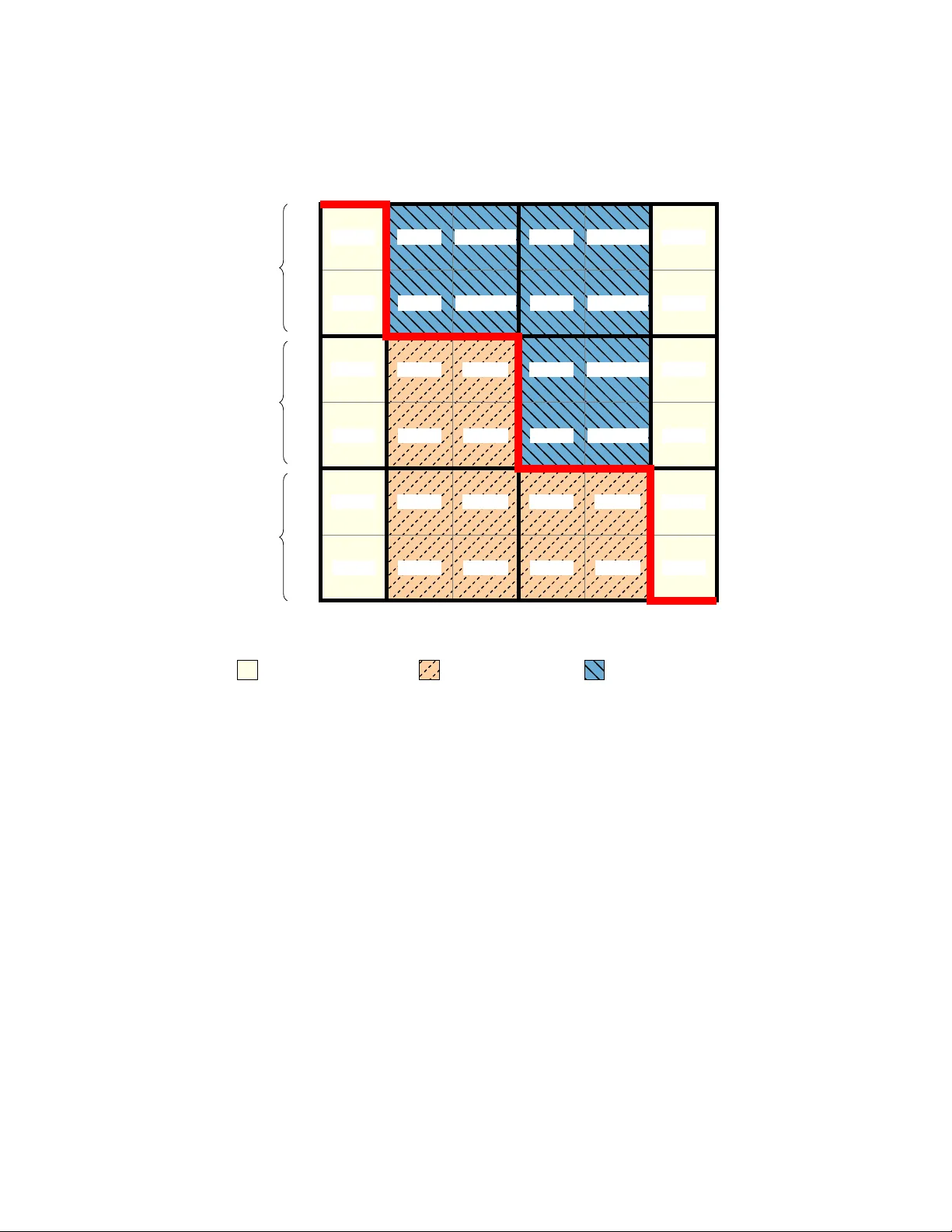
CO ALESCING RANDOM W ALKS VIA THE CO ALESCENCE DETERMINANT PIOTR ŚNIADY Abstract. When identical particles on a line collide, they merge and con tin ue as one. Exact determinantal formulas hav e long been av ailable for particles conditioned never to collide, but collisions change the number of particles, and exact distributions for the surviv ors hav e b een obtained only in specific settings and by ad ho c metho ds. Building on the coalescence determinant introduced in a companion pap er, we study the wall-particle system: the joint system of survivors and the b oundaries b etw een their basins of attraction, starting from every site occupied. Its finite-dimensional distributions are determinants of block matrices built from transition probabilities and their cum ulative sums; a finite blo ck matrix suffices even when the initial configuration is infinite. As applications, we recov er the Rayleigh spacing density and the joint distribution of consecutive gaps—which are negatively correlated—by new metho ds, and give a new deriv ation of the determinantal formula for the joint CDF of finitely many coalescing particles starting from fixed p ositions. All formulas hold for arbitrary nearest-neighbor random w alks and their Brownian scaling limits, with no specific transition kernels required. 1. Intr oduction 1.1. Coalescing particles. When iden tical particles on a line collide, they merge and con tinue as one (Figure 1 ). This coalescence rule app ears in sev eral areas of probability and mathematical physics. In the voter mo del [ HL75 ], b oundaries b et w een opinion clusters p erform coalescing random walks; their dynamics con trols the approach to consensus. In reaction-diffusion theory ( A + A → A ), diffusing particles that merge on con tact displa y anomalous kinetics: the densit y in one dimension decays as n ( t ) ∼ t − 1 / 2 , slow er than the mean-field prediction, b ecause spatial correlations dominate at large times [ DA88 ]. Arratia [ Arr79 ] placed the infinite system on rigorous fo oting. Starting coalescing Bro wnian motions from every p oin t of R , he show ed that the surviving p opulation is lo cally finite at any p ositiv e time: the system “comes do wn from infinity .” 1.2. The coalescence determinan t. The Karlin–McGregor theorem [ KM59 ] gives exact determinantal formulas for particles that avoid collision. By contrast, exact form ulas for coalescing particles hav e b een obtained only in sp ecific settings and by ad ho c metho ds. The difficulty is that collisions change the num b er of particles, so the square matrices of Karlin–McGregor do not directly apply . 2020 Mathematics Subje ct Classific ation. Primary 60K35; Secon dary 60J65, 15A15. Key words and phrases. coalescing random walks, coalescing Brownian motions, coalescence determinant, wall-particle system, skip-free pro cess, basin b oundaries, gap distribution, Rayleigh distribution, determinantal formula. 1 2 PIOTR ŚNIADY time Figure 1. Coalescing random walks starting from every site of a lattice segment. Paths merge on contact; the surviving p opulation thins ov er time. 1.2.1. The formula. The companion pap er [ Śni26a , Section Inte gr ating out the ghosts ] introduces the coalescing coun terpart: the c o alesc enc e determinant . Giv en a c o alesc enc e p attern —whic h of the n initial particles merge into eac h surviv or— the coalescence determinan t giv es the joint distribution of survivor p ositions as the determinant of an n × n matrix built from transition probabilities and their cum ulative sums (Section 2 recalls the precise definition). Muc h of the p ow er of the original Karlin–McGregor theorem comes from the w eakness of its assumptions: the Marko v prop erty and skip-free tra jectories (so that particles cannot change order without first meeting). No symmetry and no sp ecific transition kernels are needed. The coalescence determinant operates under exactly the same assumptions, and therefore applies wherever Karlin–McGregor do es: w e w ork with coalescing skip-free random walks on Z and their Brownian scaling limits on R . Concurren tly and indep endently , Urbán [ Urb25 ] pro ved the same formula for binary coalescence of Pólya walks —a sp ecial case, since Póly a w alks are birth- and-death chains. His pro of reaches the determinant from the opp osite direction, starting from Karlin–McGregor for non-colliding walks and handling coalescence via a total-probability decomp osition; see [ Śni26a ] for a detailed comparison. 1.2.2. This p ap er. This pap er explores what the coalescence determinant yields for general skip-free pro cesses, without additional lattice assumptions; a companion pa- p er [ Śni26b ] develops the richer theory av ailable when the lattice has a c hec k erb oard structure. Under the maximal en trance la w (ev ery site initially o ccupied), we study the wal l-p article system : the joint system of surviv ors and the b oundaries b etw een their basins of attraction. The coalescence determinant yields the finite-dimensional marginals of this system in closed form (Theorem 1.1 ); gap distributions follow by marginalizing ov er wall p ositions. Separately , for any finite initial configuration, the COALESCING RANDOM W ALKS VIA THE COALESCENCE DETERMINANT 3 · · · · · · · · · · · · time t = 0 t > 0 0 x − 1 / 2 x 1 / 2 x 3 / 2 y − 1 y 0 y 1 y 2 basin of y − 1 basin of y 0 basin of y 1 basin of y 2 Figure 2. The ( X , Y ) system for coalescing random walks. Paths coalesce on meeting; line w eight increases with each merger. Bottom: basin b oundaries X = ( . . . , x − 1 / 2 , x 1 / 2 , x 3 / 2 , . . . ) (triangles) partition the initial line, with x − 1 / 2 < 0 ≤ x 1 / 2 . T op: surviv or positions Y = ( . . . , y − 1 , y 0 , y 1 , y 2 , . . . ) (circles), one per basin. coalescence determinant gives W arren’s determinantal CDF formula for survivor p ositions (Theorem 6.1 ). 1.3. The wall-particle system. 1.3.1. The c onstruction. W e work under the maximal entrance la w: ev ery site of Z is initially o ccupied (for Brownian motion, every p oin t of R ). Each surviving particle then owns a b asin : the contiguous set of initial p ositions whose particles merged into it. The basins partition the initial configuration, and their b oundaries are the wal ls . The joint system of wall p ositions X and survivor p ositions Y —the wal l-p article system (Section 3 ; see Figure 2 )—pairs each survivor with its basin b oundaries. Previous work has fo cused on the survivor p ositions Y alone. Arratia [ Arr79 ] iden tified the basin b oundaries (his “partition p oints”): the p oints separating groups of initial p ositions that merge into the same survivor. F or Brownian motion, he pro ved X d = Y via a time-reversal dualit y—but this distributional identit y requires sp ecific symmetry of the underlying pro cess. W e take a differen t approac h: the join t system ( X , Y ) , pairing each survivor with its basin b oundaries, is a simpler and more natural ob ject than either marginal alone. 1.3.2. Corr elation function. The coalescence determinant giv es the finite-dimensional marginals of ( X , Y ) in closed form. Theorem 1.1 (W all-particle correlation function) . Consider a c o alescing skip-fr e e pr o c ess on Z with every site initial ly o c cupie d. The pr ob ability that ( X , Y ) c ontains the c onse cutive p attern y 0 ↖ x 1 / 2 ↗ y 1 ↖ · · · ↖ x k − 1 / 2 ↗ y k 4 PIOTR ŚNIADY (wal ls at x 1 / 2 , . . . , x k − 1 / 2 flanke d by survivors at y 0 , . . . , y k ) e quals det ( ˜ M ) , wher e ˜ M is the 2 k × 2 k blo ck matrix describ e d in Se ction 3.2 . The formula holds for any skip-free pro cess—no symmetry of the transition prob- abilities and no sp ecific kernels are needed. Despite the infinite initial configuration (ev ery site o ccupied), k consecutiv e wall-particle pairs dep end only on a 2 k × 2 k blo c k matrix; the rest of the infinite system do es not enter the formula. 1.4. Gap distributions. Marginalizing the correlation function o ver wall p osi- tions giv es the join t distribution of consecutive gaps betw een survivors. Gap distributions for coalescing Brownian motions w ere first studied b y Do ering and b en-A vraham [ DA88 ] via the inter-p article distribution function (IPDF) metho d: the rescaled nearest-neighbor distance density con verges to x e − cx 2 , a Rayleigh form. Ben-A vraham [ A vr98 ] extended the metho d to derive the full hierarch y of empt y-interv al probabilities; b en-A vraham and Brunet [ AB05 ] extracted explicit densities for tw o and three consecutive spacings. These form ulas require the explicit transition kernel of Brownian motion and grow rapidly in complexity . In the asymp- totic regime, FitzGerald, T rib e, and Zab oronski [ FTZ22 ] computed gap exp onen ts via F redholm Pfaffian metho ds, rigorously confirming predictions of Derrida and Zeitak. 1.4.1. Discr ete gap formula. In the discrete setting, no limiting pro cedure is needed. Theorem 1.2 (Discrete gap intensit y measure) . L et P s ( n ) denote the tr ansition pr ob ability of a tr anslation-invariant skip-fr e e pr o c ess on Z (fr om 0 to n in time s ), and supp ose the pr o c ess is symmetric: P s ( n ) = P s ( − n ) . Start with every site o c cupie d. The gap intensity me asur e—the exp e cte d numb er of gaps of size g p er unit length— is µ ( { g } ) = P 2 t ( g − 1) − P 2 t ( g + 1) , g = 1 , 2 , 3 , . . . The total intensity X g µ ( { g } ) = P 2 t (0) + P 2 t (1) is the survivor density p er site; dividing by it r e c overs the gap pr ob ability mass function (The or em 5.1 ). This form ula holds for any symmetric skip-free pro cess: simple random w alk, lazy random walk, or an y birth-death chain with symmetric rates. The only inputs are transition probabilities at doubled time—no PDEs, no passage to a contin uous limit. F or non-symmetric pro cesses, the gap intensit y is a conv olution of transition probabilities at the original time (Section 5.1.1 ). 1.4.2. Br ownian gaps: the R ayleigh distribution. P assing to Bro wnian motion, the discrete formula b ecomes a contin uous density . Theorem 1.3 (Single gap intensit y measure) . Under the maximal entr anc e law, the gap intensity me asur e in r esc ale d c o or dinates ( G = gap / √ t ) has density µ ( dG ) = G 2 √ π e − G 2 / 4 dG, G > 0 . COALESCING RANDOM W ALKS VIA THE COALESCENCE DETERMINANT 5 The total intensity Z ∞ 0 µ ( dG ) = 1 √ π gives the r esc ale d survivor density; un-r esc aling yields density n ( t ) = 1 / √ π t . Nor- malizing to a pr ob ability distribution gives Rayleigh( √ 2) . This reco vers the Rayleigh la w of Doering and ben-A vraham [ D A88 ] b y new metho ds (Section 5.1 ). In Section 5.1.2 we sketc h how the discrete form ula from Theorem 1.2 conv erges to this density under diffusive scaling. 1.4.3. Joint gap distribution. The single-gap Ra yleigh la w determines the marginal distribution but says nothing ab out correlations b etw een neighboring gaps. Theorem 1.4 (Join t gap intensit y) . F or two c onse cutive gaps G 1 and G 2 , the joint gap intensity h ( G 1 , G 2 ) is given by an explicit inte gr al formula (The or em 5.4 ). The mar ginal intensities ar e e ach Ra yleigh ( √ 2 ) , but the gaps ar e ne gatively c orr elate d ( ρ ≈ − 0 . 163 ). The joint density of tw o consecutive spacings w as previously obtained by b en- A vraham and Brunet [ AB05 ] from the IPDF hierarch y; we give an alternativ e deriv ation via a 4 × 4 determinant. 1.5. W arren’s formula. W arren [ W ar07 ] prov ed that for finitely many coalescing Bro wnian motions, the joint CDF of survivor p ositions is a determinant of Gaussian CDF s and their tails. Assiotis, O’Connell, and W arren [ AO W19 ] extended this to general one-dimensional diffusions and contin uous-time birth-death chains. Unlike the wall-particle correlation function—whic h requires the maximal en trance la w (ev ery site o ccupied)—W arren’s form ula applies to any finite configuration of particles at fixed starting positions. The coalescence determinant yields the CDF form ula for an y skip-free pro cess, including discrete-time random walks on Z (Theorem 6.1 ): the pro of uses only the coalescence determinant and a summation-by-parts iden tity . 1.6. Organization. Section 2 recalls the coalescence determinan t for arbitrary patterns. Section 3 dev elops the wall-particle system and derives its correlation function for skip-free pro cesses on Z . Sp ecializing to Bro wnian motion (Section 4 ), eac h pair of flanking sites collapses to a density–deriv ativ e pair as the lattice spacing v anishes, and the maximal en trance la w pro vides translation in v ariance. Gap distributions (Section 5 ) follo w by marginalizing the correlation function ov er wall p ositions for k = 1 and k = 2 . W arren’s formula (Section 6 ) is a separate application of the coalescence determinant: summing o ver all coalescence patterns conv erts densit y columns to CDF columns. 2. The Co alescence Determinant W e recall the coalescence determinant from [ Śni26a ], which applies to any finite collection of coalescing skip-free particles. W e state the formula in the discrete setting; the contin uous extension is recalled in Section 4 . W rite P ( x, y ) for the transition probabilit y of the underlying skip-free pro cess from x to y in time t (with t fixed throughout), and F ( x, y ) = X z ≤ y P ( x, z ) 6 PIOTR ŚNIADY for the cumulativ e sum. Start n particles at p ositions x 1 < x 2 < · · · < x n . A c o alesc enc e p attern is an in teger comp osition n 1 + n 2 + · · · + n k = n : the first n 1 initial particles merge into surviv or 1 , the next n 2 in to surviv or 2 , and so on. The l th blo ck of the comp osition— the initial particles merging into survivor l —has indices n 1 + · · · + n l − 1 + 1 through n 1 + · · · + n l . W rite y 1 , . . . , y k for the survivor p ositions at time t . Definition 2.1 (Coalescence matrix) . Both ro ws and columns of the n × n c o alesc enc e matrix ˜ M are indexed by { 1 , . . . , n } . The entry in ro w i , column j (where j lies in the l th blo ck, with surviv or p osition y l ) is ˜ M ij = ( P ( x i , y l ) if j is the first index in its blo ck , F ( x i , y l ) − [ i < j ] otherwise . The first column of eac h block contains transition probabilities P ; the remaining n l − 1 columns contain cumulativ e sums F with a staircase shift. Theorem 2.2 (Coalescence determinan t [ Śni26a ]) . Under the c o alesc enc e p attern n 1 + · · · + n k = n , the joint pr ob ability of survivor p ositions at y 1 < · · · < y k is det( ˜ M ) . The formula ab o v e is stated for discrete state spaces. F or contin uous pro cesses satisfying the Karlin–McGregor assumptions (such as Brownian motion), transition probabilities P b ecome densities and cumulativ e sums F b ecome CDF s; the deter- minan t then gives a probabilit y density rather than a probabilit y mass. See [ Śni26a ] for the general statemen t cov ering b oth cases. Example 2.3 (Pattern 2 + 1 ) . Three particles; the first t wo merge (surviv or y 1 ), the third survives alone ( y 2 ): ˜ M = P ( x 1 , y 1 ) F ( x 1 , y 1 ) − 1 P ( x 1 , y 2 ) P ( x 2 , y 1 ) F ( x 2 , y 1 ) P ( x 2 , y 2 ) P ( x 3 , y 1 ) F ( x 3 , y 1 ) P ( x 3 , y 2 ) . 3. The W all-P ar ticle System 3.1. T w o coupled sequences. Consider a coalescing skip-free pro cess on Z with ev ery site initially occupied. When tw o particles meet, they coalesce and contin ue as one. Fix a time t > 0 . W e call eac h surviving particle a survivor and write Y = ( y j ) j ∈ Z for the increasing sequence of survivor p ositions (time- t co ordinates), indexed by the in tegers. Eac h surviv or o wns a b asin : the contiguous set of initial p ositions whose particles merged into it. The basins partition Z . Betw een consecutiv e basins lies a wal l : the half-in teger separating the last initial position in one basin from the first in the next. W rite X = ( x i ) i ∈ Z ′ for the increasing sequence of w alls (time- 0 co ordinates), where Z ′ = Z + 1 2 . T he basin of y j is the set of initial integers in the in terv al ( x j − 1 / 2 , x j + 1 / 2 ) . Throughout, X and Y denote the random sequences, with comp onen ts x i and y j . When x i and y j app ear without b oldface in formulas, they denote sp ecific (deterministic) p ositions. See Figure 2 for an illustration. Because walls liv e at time 0 and surviv ors at time t , there is no in terlacing constrain t on their v alues—a surviv or need not lie inside its basin. The t wo sequences hav e interlea ved indices—half-integers for walls, integers for survivors: · · · ↖ x 1 / 2 ↗ y 1 ↖ x 3 / 2 ↗ y 2 ↖ x 5 / 2 ↗ · · · COALESCING RANDOM W ALKS VIA THE COALESCENCE DETERMINANT 7 W e use this zigzag notation throughout: each arrow connects a wall to an adjacent surviv or in the index order. R emark 3.1 (Lab eling con ven tion) . The lab eling of w alls and survivors is determined only up to a global shift of the index set. When needed, we fix a reference b y requiring x − 1 / 2 < 0 ≤ x 1 / 2 , placing the origin in the basin of y 0 . This conv ention pla ys no role in the distributional results. Eac h wall x i ( i ∈ Z ′ ) is flanked b y tw o initial integer positions: a i = x i − 1 2 , b i = x i + 1 2 . P osition a i (to the left of the wall) b elongs to the basin of surviv or y i − 1 / 2 , and b i (to the right) to the basin of survivor y i + 1 / 2 . 3.2. Correlation function. Theorem 3.2 (W all-particle correlation function) . Consider a c o alescing skip-fr e e pr o c ess on Z with every site initial ly o c cupie d. F or p ositions x 1 / 2 < · · · < x k − 1 / 2 and y 0 < · · · < y k , the pr ob ability that ( X , Y ) c ontains the c onse cutive p attern y 0 ↖ x 1 / 2 ↗ y 1 ↖ x 3 / 2 ↗ · · · ↖ x k − 1 / 2 ↗ y k e quals det ( ˜ M ) , wher e ˜ M is the c o alesc enc e matrix (Definition 2.1 ) for 2 k p articles starte d at a 1 , b 1 , . . . , a k , b k with c o alesc enc e p attern 1 + 2 + · · · + 2 + 1 : p article a 1 survives alone at y 0 ; e ach p air ( b l , a l +1 ) mer ges into survivor y l ; and b k survives alone at y k . Pr o of. Consider first only the 2 k flanking particles a 1 , b 1 , . . . , a k , b k (no other sites o ccupied; see Figure 3 for k = 2 ). The coalescence determinant (Theorem 2.2 ) gives the probability of the stated coalescence even t as det( ˜ M ) . No w p opulate every remaining integer site. In Arratia’s construction of coalescing pro cesses [ Arr79 ], additional particles do not alter the tra jectories of existing ones: they follow the same underlying paths and merge into whatev er they meet. Because the pro cess is skip-free, ev ery in termediate particle (at a site betw een b l and a l +1 ) is trapp ed b etw een the con v erging paths of b l and a l +1 and must coalesce in to the same surviv or y l (see Figure 3 ). The wall-particle ev en t in the full system therefore has the same probabilit y as the coalescence even t for the 2 k flanking particles alone. □ 3.3. Block structure. W e now examine the matrix ˜ M from Theorem 3.2 more closely . The pattern 1 + 2 + · · · + 2 + 1 gives ˜ M a 2 × 2 blo ck structure: eac h wall con tributes a ro w-pair and eac h interior surviv or a column-pair ( P and F ), while the tw o b oundary survivors contribute single P columns. W rite B i,j ( i ∈ Z ′ , j ∈ Z ) for the 2 × 2 blo ck at row-pair i (w all) and column-pair j (survivor): B i,j = P ( a i , y j ) F ( a i , y j ) − [ i < j ] P ( b i , y j ) F ( b i , y j ) − [ i < j ] ! , where [ i < j ] is the Iverson brac ket. Example 3.3 (P attern 1+2+1 ) . F or k = 2 (tw o walls, three surviv ors), the pattern y 0 ↖ x 1 / 2 ↗ y 1 ↖ x 3 / 2 ↗ y 2 giv es a 4 × 4 matrix with column structure 1 + 2 + 1 . The interior survivor y 1 con tributes a blo ck B i,j —a P column and an F column 8 PIOTR ŚNIADY t = 0 t > 0 time a 1 b 1 a 2 b 2 x 1 / 2 x 3 / 2 y 0 y 1 y 2 pair 1 (solid) pair 2 (zigzag) survivor (double) intermediate Figure 3. Pro of of Theorem 3.2 for k = 2 . The coalescence determi- nan t applies to the four flanking particles a 1 , b 1 , a 2 , b 2 (b old paths: solid for pair 1 , zigzag for pair 2 ). P articles b 1 and a 2 coalesce in to surviv or y 1 (double line); particles a 1 and b 2 surviv e as y 0 and y 2 . The intermediate particles (thin gray) cannot cross the flanking paths—the skip-free prop ert y traps them in the closing funnel b et ween b 1 and a 2 —so they are absorb ed into the same surviv ors. A dding them do es not c hange the coalescence outcome for the flanking particles. carrying a staircase step—while the b oundary survivors y 0 and y 2 eac h contribute a single P column: ˜ M = P ( a 1 , y 0 ) P ( a 1 , y 1 ) F ( a 1 , y 1 ) − 1 P ( a 1 , y 2 ) P ( b 1 , y 0 ) P ( b 1 , y 1 ) F ( b 1 , y 1 ) − 1 P ( b 1 , y 2 ) P ( a 2 , y 0 ) P ( a 2 , y 1 ) F ( a 2 , y 1 ) P ( a 2 , y 2 ) P ( b 2 , y 0 ) P ( b 2 , y 1 ) F ( b 2 , y 1 ) P ( b 2 , y 2 ) . F or the b oundary case k = 1 (one w all, no in terior surviv ors, no coalescence at all), there are no blo c ks B i,j and the matrix reduces to the 2 × 2 Karlin–McGregor determinan t [ KM59 ]. Corollary 3.4 (Blo ck structure of ˜ M ) . The matrix ˜ M fr om The or em 3.2 for a p attern with k wal ls has a c olumn structur e 1 + 2 + · · · + 2 + 1 : the first and last c olumns ar e single P c olumns (one for e ach b oundary survivor), and e ach interior survivor c ontributes a 2 × 2 blo ck B i,j . Se e Figur e 4 for the k = 3 c ase, wher e the blo ck structur e and the stair c ase p attern ar e ful ly app ar ent. R emark 3.5 (Staircase and blo ck structure) . The blo ck formula for B i,j uses the Iv erson brac ket [ i < j ] , whic h steps at blo ck b oundaries. The coalescence matrix (Definition 2.1 ), ho wev er, defines the staircase at the level of individual rows. F or the wall-particle patterns 1 + 2 + · · · + 2 + 1 , each staircase step falls betw een the t wo rows of a single blo c k, so the tw o con ven tions agree on all F columns (where the distinction matters) and ma y differ only on P columns—but P en tries do not dep end on the staircase. W arren’s formula (Section 6 ), how ever, sums ov er all 2 n − 1 coalescence patterns and requires the original row-lev el staircase. R emark 3.6 (Asymmetry b et w een w alls and survivors) . The blo ck matrix ˜ M treats w alls and surviv ors asymmetrically: the pattern has k w alls but k + 1 survivors, and COALESCING RANDOM W ALKS VIA THE COALESCENCE DETERMINANT 9 p a 1 ( y 0 ) p a 1 ( y 1 ) F a 1 ( y 1 ) − 1 p a 1 ( y 2 ) F a 1 ( y 2 ) − 1 p a 1 ( y 3 ) p b 1 ( y 0 ) p b 1 ( y 1 ) F b 1 ( y 1 ) − 1 p b 1 ( y 2 ) F b 1 ( y 2 ) − 1 p b 1 ( y 3 ) p a 2 ( y 0 ) p a 2 ( y 1 ) F a 2 ( y 1 ) p a 2 ( y 2 ) F a 2 ( y 2 ) − 1 p a 2 ( y 3 ) p b 2 ( y 0 ) p b 2 ( y 1 ) F b 2 ( y 1 ) p b 2 ( y 2 ) F b 2 ( y 2 ) − 1 p b 2 ( y 3 ) p a 3 ( y 0 ) p a 3 ( y 1 ) F a 3 ( y 1 ) p a 3 ( y 2 ) F a 3 ( y 2 ) p a 3 ( y 3 ) p b 3 ( y 0 ) p b 3 ( y 1 ) F b 3 ( y 1 ) p b 3 ( y 2 ) F b 3 ( y 2 ) p b 3 ( y 3 ) a 1 b 1 a 2 b 2 a 3 b 3 pair 1 pair 2 pair 3 y 0 y 1 y 2 y 3 2 × 1 2 × 2 2 × 2 2 × 1 transition prob. p cumul. sum F cumul. sum F − 1 Figure 4. Blo ck structure of ˜ M for the 1 + 2 + 2 + 1 pattern ( k = 3 w alls). Ro ws come in pairs; columns are grouped b y survivor: 2 × 1 b oundary blo c ks for y 0 and y 3 , and 2 × 2 interior blocks for y 1 and y 2 , each containing a P column and an F column. The thic k red s taircase separates F − 1 blocks (dark blue, solid hatching) from F blo c ks (orange, dashed hatching); unhatched y ellow blo c ks con tain only P entries. the tw o b oundary surviv ors each contribute only one column (rather than tw o), so w alls and survivors cannot simply b e interc hanged. When the underlying pro cess has a chec k erb oard structure—such as discrete-time ± 1 random walk—this asymmetry can b e resolved: a decomp osition of the lattice giv es a dualit y b etw een w alls and surviv ors, connecting the wall-particle system to Pfaffian p oint pro cesses. This is dev elop ed in [ Śni26b ]. 3.4. Examples. W e describ e t w o classes of processes satisfying the skip-free as- sumption of Theorem 3.2 . Example 3.7 (Simple symmetric random w alk) . Consider the ± 1 simple random walk: at each discrete time step, every particle mov es left or right with equal probability . Space-time splits in to t wo chec k erb oard sublattices: a particle at position x at 10 PIOTR ŚNIADY time t satisfies either x + t ≡ 0 or x + t ≡ 1 ( mo d 2) , and eac h particle stays on one sublattice forever. If we start particles at every site of Z , the Karlin–McGregor assumptions fail: a particle starting at an even site and a particle starting at an o dd site live on complementary sublattices and can exc hange order without ever sharing a site, so the non-crossing prop erty do es not hold. The remedy is to o ccup y a single sublattice—say all ev en sites 2 Z at time 0 . P articles on the same sublattice cannot cross without meeting (they share the same parity at every time step), so the skip-free assumption holds. Applying the framew ork to the initial sublattice 2 Z (with spacing 2 playing the role of the unit lattice), walls sit at the o dd integers 2 Z + 1 . A t time t , all survivors share the same parit y , so all gaps b etw een consecutive surviv ors are even (see Theorem 5.1 for the gap distribution). Example 3.8 (Birth-death chains) . Contin uous-time birth-death chains on { 0 , 1 , 2 , . . . } are skip-free by construction (only ± 1 transitions), and every in teger is a v alid state at every time—no parity constrain t. The wall-particle framew ork applies directly , with walls at { 1 2 , 3 2 , . . . } . F or instance, the M/M/1 queue has transition probabilities expressible via mo dified Bessel functions [ KM59 ]. 3.5. Multi-pattern correlations. Theorem 3.2 extends to sev eral separated consec- utiv e patterns observed simultaneously , with an unsp ecified num b er of in termediate surviv ors betw een them. W e state this for completeness; it is not used in the presen t pap er. Theorem 3.9 (Multi-pattern correlation function) . Consider m sep ar ate d c onse cu- tive p atterns in the wal l-p article system. Pattern α ( α = 1 , . . . , m ) c onsists of k α wal ls and k α + 1 survivors: y ( α ) 0 ↖ x ( α ) 1 / 2 ↗ y ( α ) 1 ↖ · · · ↖ x ( α ) k α − 1 / 2 ↗ y ( α ) k α , with wal ls and survivors e ach glob al ly incr e asing. Betwe en c onse cutive p atterns, the numb er of interme diate survivors is unsp e cifie d. The pr ob ability that ( X , Y ) c ontains al l m p atterns simultane ously e quals det ( ˜ M ) , wher e ˜ M is the c o alesc enc e matrix (Definition 2.1 ) for the 2 K flanking p articles ( K = P α k α ). Within e ach p attern, the c o alesc enc e is as in The or em 3.2 ; b etwe en c onse cutive p atterns, the b oundary p articles survive alone. Pr o of. Apply the coalescence determinant (Theorem 2.2 ) to the 2 K flanking p o- sitions. Within each pattern, the argument is identical to Theorem 3.2 . Bet ween patterns, intermediate particles are trapp ed b etw een the last flanking particle of one pattern and the first of the next, so p opulating them do es not change the probabilit y . □ Example 3.10 (T w o separated patterns) . Consider m = 2 patterns: pattern 1 with k 1 = 2 (w alls x 1 / 2 , x 3 / 2 , flanking p ositions a 1 , b 1 , a 2 , b 2 , surviv ors y 0 , y 1 , y 2 ) and pattern 2 with k 2 = 1 (wall x 5 / 2 , flanking p ositions a 3 , b 3 , survivors y 3 , y 4 ), with an unsp ecified num b er of in termediate survivors b etw een y 2 and y 3 . The 6 × 6 matrix COALESCING RANDOM W ALKS VIA THE COALESCENCE DETERMINANT 11 is: ˜ M = y 0 y 1 y 2 y 3 y 4 a 1 P P F − 1 P P P b 1 P P F − 1 P P P a 2 P P F P P P b 2 P P F P P P a 3 P P F P P P b 3 P P F P P P . Here P denotes a transition probabilit y entry P ( a l , y j ) or P ( b l , y j ) , and F , F − 1 denote cumulativ e sum en tries F ( · , y 1 ) or F ( · , y 1 ) − 1 . The double lines mark the pattern b oundary . Within pattern 1 (upp er-left 4 × 4 blo c k), the structure is the familiar 1 + 2 + 1 from Example 3.3 : the interior surviv or y 1 has an F column, with the staircase separating F − 1 (w all 1 , ab o ve) from F (w alls 2 and 3 , b elow). P attern 2 (low er-right 2 × 2 blo ck) is pure Karlin–McGregor. The off-diagonal blo c ks couple the tw o patterns; their entries are all P . No F column app ears betw een y 2 and y 3 : this absence is what allows an arbitrary n umber of unsp ecified intermediate surviv ors b etw een the tw o patterns. Compare Figure 4 , where the single pattern 1 + 2 + 2 + 1 has F columns for every in terior surviv or. 4. Br o wnian Motion Setting W e specialize the blo ck matrix ˜ M (Corollary 3.4 ) to Brownian motion. In the contin uous limit, each flanking pair ( a l , b l ) collapses to a single wall p osition; subtracting the tw o ro ws of eac h blo c k and dividing b y the grid spacing turns the ro w pair in to a Gaussian density and its spatial deriv ative. The resulting 2 k × 2 k matrix M 0 is explicit and clean. W e then pass to the maximal entrance la w—coalescing Brownian motions starting from all of R , a classical construction due to Arratia [ Arr79 ]—and obtain a determinantal formula for the in tensity of the w all-particle system. 4.1. T ransition densities. W rite p x ( y ) for the Gaussian transition density at time t (fixed throughout): p x ( y ) = 1 √ 2 π t exp − ( y − x ) 2 2 t , and F x ( y ) for the Gaussian CDF: F x ( y ) = Z y −∞ p x ( z ) dz = Φ y − x √ t , where Φ is the standard normal CDF. Start coalescing Brownian motions from a grid with spacing ε . Eac h w all is flank ed by starting p ositions a l and b l = a l + ε . The coalescence determinan t (Theorem 2.2 ) giv es a 2 k × 2 k matrix as in Section 3.2 , with Bro wnian densities p x ( y ) and CDF s F x ( y ) in place of P ( x, y ) and F ( x, y ) . Subtracting the a l ro w from the b l ro w within eac h pair (which preserves the determinan t) and dividing by ε replaces the second row by the deriv ativ e ∂ x , up to 12 PIOTR ŚNIADY O ( ε ) error. Eac h 2 × 2 interior blo c k b ecomes: p x ( y ) F x ( y ) − [ · ] ∂ x p x ( y ) ∂ x F x ( y ) ! + O ( ε ) , where [ · ] stands for the Iverson brack et as in B i,j (Section 3.3 ). The boundary columns (containing only p en tries) undergo the same row op eration, becoming ( p x ( y ) , ∂ x p x ( y )) T . Each row-pair contributes one factor of ε . Prop osition 4.1 (Grid refinement) . F or c o alescing Br ownian motions starting fr om a grid with sp acing ε , the wal l-p article c orr elation function for k wal ls ne ar x 1 / 2 , . . . , x k − 1 / 2 and k + 1 survivors ne ar y 0 , . . . , y k e quals ε k det ( M 0 ) + O ( ε k +1 ) , wher e M 0 is the 2 k × 2 k matrix with alternating density and derivative r ows and the c olumn structur e of ˜ M . Each wal l c ontributes one factor of ε . Pr o of. The row op erations ab ov e giv e det( ˜ M ) = ε k det( M 0 ) + O ( ε k +1 ) . □ R emark 4.2 (W ronskian structure) . F or translation-inv arian t kernels p x ( y ) = p ( y − x ) , ∂ x p x ( y ) = − ∂ y p x ( y ) , ∂ x F x ( y ) = − p x ( y ) . Th us the deriv ativ e ro w of each blo ck in M 0 is − ∂ y applied to the density row, giving a generalized W ronskian in the CDF F x ev aluated at y . This structure matc hes the T ribe–Zab oronski kernel for coalescing Bro wnian motions [ TZ11 ; GPTZ18 ]; the connection is explored in [ Śni26b ]. 4.2. Maximal en trance law. Arratia [ Arr79 ] constructs coalescing Brownian motions starting from all of R via dyadic approximation and pro v es that the set of surviv ors is lo cally finite. W e use the same construction to build the joint ( X , Y ) system. Fix a time t > 0 . A t step n = 0 , 1 , 2 , . . . , start indep enden t Brownian motions from every p oin t of 2 − n Z at time 0 , and run them until time t with the coalescing rule: when tw o tra jectories meet, they merge and contin ue as one. The construction is incremental. Going from step n to step n + 1 , the new starting p oin ts 2 − n − 1 (2 Z + 1) interlea ve the existing ones from 2 − n Z . Eac h newly launched Bro wnian motion either hits an existing tra jectory b efore time t and is absorbed, or survives to time t without hitting any existing tra jectory . The set of survivors gro ws monotonically with n : existing survivors are nev er remo v ed. The limiting set is lo cally finite: t w o Brownian motions distance ε apart fail to coalesce by time t with probability ε/ √ π t + O ( ε 2 ) (this is Arratia’s estimate [ Arr79 ]; it also follows from Prop osition 4.1 with k = 1 ), so the exp ected num b er of surviv ors p er unit length remains b ounded as the grid refines. The construction pro duces the ( X , Y ) system from Section 3 : walls X = ( x i ) (basin boundaries) and surviv ors Y = ( y j ) (p ositions at time t ), with basins partitioning R . The maximal entrance law inherits translation inv ariance from the dy adic grid: the shifts b y 2 − n b ecome dense as n → ∞ , so the joint la w of ( X , Y ) is inv arian t under all translations of R . 4.3. W all-particle intensit y. A consecutiv e pattern with k w alls and k +1 survivors liv es in R 2 k +1 ( k w all co ordinates plus k + 1 survivor c oordinates), and the wall- particle system under the maximal entrance la w forms a p oin t pro cess on this space. Its intensity is the density of the p oint process with resp ect to Leb esgue measure: in tegrating ov er a region gives the expected num b er of patterns in that region. COALESCING RANDOM W ALKS VIA THE COALESCENCE DETERMINANT 13 Com bining the grid-refinement limit (Prop osition 4.1 ) with the dyadic construction giv es this intensit y in closed form. Theorem 4.3 (W all-particle in tensity) . Under the maximal entr anc e law for c o a- lescing Br ownian motions at time t > 0 , the c onse cutive p attern y 0 ↖ x 1 / 2 ↗ y 1 ↖ · · · ↖ x k − 1 / 2 ↗ y k has intensity det M 0 ( x 1 / 2 , . . . , x k − 1 / 2 ; y 0 , . . . , y k ) with r esp e ct to L eb esgue me asur e on R 2 k +1 , wher e M 0 is the 2 k × 2 k matrix fr om Pr op osition 4.1 . Pr o of. A t dy adic step n , the starting grid has spacing ε = 2 − n . By Prop osition 4.1 , the wall-particle correlation function for k w alls near x 1 / 2 , . . . , x k − 1 / 2 and survivors near y 0 , . . . , y k is ε k det ( M 0 ) + O ( ε k +1 ) . Each factor of ε matc hes the grid spacing p er wall, so det ( M 0 ) is the density p er unit length in each w all co ordinate. Since the survivor set is lo cally finite [ Arr79 ] and grows monotonically with each dyadic refinemen t, it almost surely stabilizes on any bounded interv al after finitely many steps. Passing to n → ∞ gives the result. □ 4.4. Example: reflected Brownian motion. The grid-refinement tec hnique of Section 4.1 extends naturally to any pro cess with contin uous paths and a smo oth transition density . As an illustration b ey ond standard Brownian motion, we treat coalescing Bro wnian motions on the half-line [0 , ∞ ) with reflection at 0 . T ranslation in v ariance is lost, and the reflecting b oundary in tro duces a leftmost survivor with a sp ecial role. Reflected Brownian motion on [0 , ∞ ) has transition density p t ( x, y ) = 1 √ 2 π t h e − ( y − x ) 2 / (2 t ) + e − ( y + x ) 2 / (2 t ) i , x, y ≥ 0 . This is skip-free (contin uous paths), so the coalescence determinant applies. The maximal entrance law o ccupies all of [0 , ∞ ) ; translation inv ariance is broken by the b oundary at 0 . The set of survivors is half-infinite: there is a leftmost surviv or y 0 , with basin [0 , x 1 / 2 ) b ounded on the left b y the reflecting b oundary . W e write y 0 ↖ x 1 / 2 ↗ y 1 ↖ x 3 / 2 ↗ y 2 ↖ · · · for the wall-particle system, with w alls 0 < x 1 / 2 < x 3 / 2 < · · · and surviv ors 0 < y 0 < y 1 < y 2 < · · · . Theorem 4.4 (Half-line intensit y) . Under the maximal entr anc e law for r efle cte d Br ownian motion on [0 , ∞ ) at time t > 0 , the p attern y 0 ↖ x 1 / 2 ↗ y 1 ↖ · · · ↖ x k − 1 / 2 ↗ y k with y 0 the leftmost survivor has intensity det M 0 ( x 1 / 2 , . . . , x k − 1 / 2 ; y 0 , . . . , y k ) with r esp e ct to L eb esgue me asur e on (0 , ∞ ) 2 k +1 . Her e M 0 is a (2 k + 1) × (2 k + 1) matrix: its first r ow c omes fr om a p article at the b oundary 0 , and its r emaining k r ow-p airs ar e the density and ∂ x -derivative r ows fr om the k wal ls. Columns ar e or ganize d as in the c o alesc enc e p attern 2 + 2 + · · · + 2 + 1 : a P -and- F c olumn-p air for e ach gr oup of size 2 , and a single P c olumn for the final gr oup of size 1 . 14 PIOTR ŚNIADY Pr o of. Construct the maximal entrance law on [0 , ∞ ) by dyadic approximation, as in Section 4.2 : at step n , start reflected Brownian motions from every p oin t of { 0 , 2 − n , 2 · 2 − n , . . . } . A t grid spacing ε = 2 − n , the particle at 0 and the 2 k flanking particles a 1 , b 1 , . . . , a k , b k form a system of 2 k + 1 particles. The coalescence determinant (Theorem 2.2 ) gives their joint distribution under the pattern 2 + 2 + · · · + 2 + 1 : the particle at 0 and a 1 merge in to y 0 ; each pair ( b l , a l +1 ) merges into y l ; and b k surviv es alone at y k . In termediate particles are trapp ed by the skip-free property (as in Theorem 3.2 ): b et ween 0 and a 1 , the reflecting b oundary preven ts leftw ard escap e; b et w een b l and a l +1 , the closing funnel absorbs all intermediate particles. The grid-refinement pro cedure (Prop osition 4.1 ) carries ov er: eac h ( a l , b l ) pair collapses to a density row and a ∂ x -deriv ativ e ro w, con tributing one factor of ε ; the particle at 0 con tributes a single ro w. Th us det( ˜ M ) = ε k det( M 0 ) + O ( ε k +1 ) . Since the survivor set is lo cally finite [ Arr79 ] and grows monotonically , it stabilizes on any b ounded interv al after finitely many steps. Passing to n → ∞ giv es the in tensity det( M 0 ) . □ Example 4.5 (One wall on the half-line) . F or k = 1 (one wall, t wo survivors, leftmost surviv or at y 0 ), the pattern 2+1 gives the 3 × 3 matrix M 0 = p 0 ( y 0 ) F 0 ( y 0 ) − 1 p 0 ( y 1 ) p x 1 / 2 ( y 0 ) F x 1 / 2 ( y 0 ) p x 1 / 2 ( y 1 ) ∂ x p x 1 / 2 ( y 0 ) ∂ x F x 1 / 2 ( y 0 ) ∂ x p x 1 / 2 ( y 1 ) , where p x ( y ) and F x ( y ) use the reflected Brownian motion transition density . The follo wing sections compute det ( M 0 ) explicitly for standard Brownian motion on R : the single gap k = 1 (Section 5.1 ) and the join t gap k = 2 (Section 5.3 ). 5. Gap Distributions W e compute gap distributions in the discrete setting (where no limiting pro cedure is needed) and for Bro wnian motion under the maximal entrance la w. All results are stated in terms of the gap intensity me asur e : µ ( { g } ) is the exp ected num b er of gaps of size g p er unit length. Dividing by the total in tensity P g µ ( { g } ) (the surviv or density) recov ers the gap probability distribution. 5.1. Single gap. W e deriv e the single-gap intensit y measure, first in the discrete setting (where the form ula is exact) and then for Bro wnian motion under the maximal en trance la w. The Bro wnian result reco vers the Rayleigh la w first obtained b y Do ering and ben-A vraham [ DA88 ] via the IPDF metho d and b y b en-A vraham [ A vr98 ]; w e give a new pro of through the wall-particle system. 5.1.1. Discr ete single-gap distribution. Apply the wall-particle system with k = 1 : a single wall at half-integer x separates tw o basins, with flanking sites a = x − 1 2 and b = x + 1 2 (so b = a + 1 ). The tw o survivors y 0 < y 1 satisfy the Karlin–McGregor non-in tersection condition, and the coalescence determinant giv es: det( ˜ M ) = P ( a, y 0 ) P ( b, y 1 ) − P ( a, y 1 ) P ( b, y 0 ) . COALESCING RANDOM W ALKS VIA THE COALESCENCE DETERMINANT 15 Summing the wall-particle in tensit y ov er all w all p ositions gives the probabilit y that y 0 and y 1 are consecutive survivors: (5.1) P ( y 0 , y 1 consecutiv e survivors ) = X a ∈ Z P ( a, y 0 ) P ( a +1 , y 1 ) − P ( a, y 1 ) P ( a +1 , y 0 ) . This formula is v alid for an y skip-free pro cess with ev ery site initially o ccupied: no translation inv ariance or symmetry is needed. T ranslation-in v arian t case. Assume P ( x, y ) = P (0 , y − x ) for all x, y ∈ Z ; we write P ( n ) = P (0 , n ) when the time t is understo o d. W riting g = y 1 − y 0 for the gap, translation inv ariance gives P ( a, y 0 ) = P ( y 0 − a ) , P ( a + 1 , y 1 ) = P ( y 1 − a − 1) , and so on; each summand in ( 5.1 ) dep ends only on g and a − y 0 , so the sum is indep enden t of y 0 . Define the auto c orr elation (5.2) R ( m ) = X s ∈ Z P t ( s ) P t ( s + m ) . Then the tw o sums in ( 5.1 ) are R ( g − 1) and R ( g + 1) resp ectively , giving (5.3) µ ( { g } ) = R ( g − 1) − R ( g + 1) . Symmetric case. When the walk is symmetric ( P ( n ) = P ( − n ) for all n ), the auto correlation reduces to a conv olution: R ( m ) = P s P ( s ) P ( m − s ) = P 2 t ( m ) b y the Chapman–Kolmogoro v identit y , so µ ( { g } ) = P 2 t ( g − 1) − P 2 t ( g + 1) . The con tinuous-time simple random walk ( ± 1 jumps, each at rate 1 ) is the main example: ev ery integer is reachable from every integer, so there is no parity constrain t. Theorem 5.1 (Discrete gap intensit y measure) . F or a symmetric tr anslation- invariant c o alescing skip-fr e e pr o c ess on Z with every site initial ly o c cupie d, the gap intensity me asur e is µ ( { g } ) = P 2 t ( g − 1) − P 2 t ( g + 1) , g = 1 , 2 , 3 , . . . The total intensity is a telesc oping sum: ∞ X g =1 µ ( { g } ) = P 2 t (0) + P 2 t (1) , sinc e P 2 t ( g ) → 0 as g → ∞ ; this gives the survivor density p er site. Dividing by the total intensity r e c overs the pr ob ability mass function P ( G = g ) = µ ( { g } ) / [ P 2 t (0) + P 2 t (1)] . Pr o of. Equation ( 5.3 ) gives µ ( { g } ) . F or the total intensit y , the partial sum N X g =1 P 2 t ( g − 1) − P 2 t ( g + 1) = P 2 t (0) + P 2 t (1) − P 2 t ( N ) − P 2 t ( N + 1) telescop es (reindex: the first sum runs o ver m = 0 , . . . , N − 1 and the second ov er m = 2 , . . . , N + 1 ). Letting N → ∞ gives total intensit y P 2 t (0) + P 2 t (1) . □ 16 PIOTR ŚNIADY 5.1.2. Sc aling limit pr eview. Under diffusiv e scaling, the discrete gap distribution from Theorem 5.1 recov ers the Bro wnian motion Ra yleigh density from Theorem 1.3 . The scaling sends: • lattice spacing ε → 0 ; • discrete gap g ∈ Z to con tinuous gap G = g · ε (measured in the rescaled co ordinates); • discrete time t to contin uous time with ε 2 t held fixed. In this regime, the transition probability P 2 t ( n ) at the integer n = ( g ± 1) is w ell appro ximated by the Gaussian densit y p ( nε, 2 ε 2 t ) times the lattice spacing ε . The difference at unit spacing b ecomes a deriv ative: P 2 t ( g − 1) − P 2 t ( g + 1) ≈ − 2 ε ∂ G p ( G, 2 T ) G = g ε, T = ε 2 t , and since ∂ G p ( G, 2 T ) = − G 2 T p ( G, 2 T ) , this gives µ ( dG ) ∝ G e − G 2 / (4 T ) dG, the gap intensit y measure, identifying the Ra yleigh( √ 2) family . This argumen t is a scaling heuristic, not a rigorous pro of: a complete deriv a- tion requires controlling the error terms in the Gaussian approximation and the con vergence of the normalizing constan ts. The rigorous Brownian motion proof follo ws. 5.2. Brownian motion single gap. W e prov e Theorem 1.3 by applying the ( X , Y ) framew ork from Section 3 (with the Brownian motion sp ecialization from Section 4.1 ) with k = 1 and passing to the maximal entrance la w (Section 4.2 ). W e recall the R ayleigh distribution with scale parameter σ > 0 : Ra yleigh( σ ) : f σ ( G ) = G σ 2 e − G 2 / (2 σ 2 ) , G > 0 . The mean is σ p π / 2 and the v ariance is (4 − π ) σ 2 / 2 . Theorem 5.2 (Gap in tensity measure under the maximal entrance law) . Under the maximal entr anc e law, the gap intensity me asur e in r esc ale d c o or dinates has density µ ( dG ) = G 2 √ π e − G 2 / 4 dG, G > 0 . Normalizing to a pr ob ability distribution gives the Ra yleigh ( √ 2 ) density f ( G ) = G 2 e − G 2 / 4 . Corollary 5.3 (Densit y of surviving particles) . The total intensity is R ∞ 0 µ ( dG ) = 1 / √ π , giving the r esc ale d survivor density. Sinc e the r esc ale d me an gap is E [ G ] = √ π , the me an gap b etwe en c onse cutive survivors at time t is √ π t , and the density of survivors p er unit length is 1 / √ π t . Pr o of of The or em 5.2 . By Theorem 4.3 with k = 1 , the intensit y of the pattern y 0 ↖ x ↗ y 1 is det( M 0 ) , where M 0 = p x ( y 0 ) p x ( y 1 ) ∂ x p x ( y 0 ) ∂ x p x ( y 1 ) . COALESCING RANDOM W ALKS VIA THE COALESCENCE DETERMINANT 17 Using ∂ x p x ( y ) = p x ( y ) · ( y − x ) /t , the determinant is: det( M 0 ) = p x ( y 0 ) p x ( y 1 ) · y 1 − y 0 t . Change coordinates: let u = y 0 − x (displacemen t of left surviv or from wall p osition) and G = y 1 − y 0 (gap). Then p x ( y 0 ) = (2 π t ) − 1 / 2 e − u 2 / (2 t ) and p x ( y 1 ) = (2 π t ) − 1 / 2 e − ( u + G ) 2 / (2 t ) , so det( M 0 ) = G 2 π t 2 exp − u 2 + ( u + G ) 2 2 t . Completing the square: u 2 + ( u + G ) 2 = 2( u + G/ 2) 2 + G 2 / 2 . Integrating ov er u : Z ∞ −∞ det( M 0 ) du = G 2 π t 2 e − G 2 / (4 t ) √ π t = G 2 √ π t 3 / 2 e − G 2 / (4 t ) . By translation in v ariance, this is independent of the location y 0 , so it gives the gap intensit y p er unit (unrescaled) length. Changing to rescaled co ordinates G = ( y 1 − y 0 ) / √ t , the gap in tensit y p er unit rescaled length b ecomes µ ( dG ) = G 2 √ π e − G 2 / 4 dG, whic h is 1 / √ π times the Ra yleigh( √ 2) density . □ 5.3. Join t distribution of consecutive gaps. W e deriv e the joint intensit y of t wo consecutive gaps, first in the discrete setting and then for Brownian motion, pro ving Theorem 1.4 . The Bro wnian joint density w as previously obtained by b en-A vraham and Brunet [ AB05 ] from the IPDF hierarch y; our deriv ation via the w all-particle system applies to any skip-free pro cess, including discrete random w alks and birth-death chains. 5.3.1. Discr ete joint gaps. F or k = 2 consecutiv e gaps, the 1 + 2 + 1 pattern from Example 3.3 gives a 4 × 4 determinant. As in the single-gap case (Section 5.1.1 ), summing the wall-particle intensit y ov er all w all p ositions gives the probabilit y that y 0 , y 1 , y 2 are consecutive survivors: P ( y 0 , y 1 , y 2 consecutiv e survivors ) = X a 1 ,a 2 ∈ Z det( ˜ M ) , where a l , b l = a l + 1 are the flanking sites of wall l , and ˜ M is the 4 × 4 matrix ˜ M = P ( a 1 , y 0 ) P ( a 1 , y 1 ) F ( a 1 , y 1 ) − 1 P ( a 1 , y 2 ) P ( b 1 , y 0 ) P ( b 1 , y 1 ) F ( b 1 , y 1 ) − 1 P ( b 1 , y 2 ) P ( a 2 , y 0 ) P ( a 2 , y 1 ) F ( a 2 , y 1 ) P ( a 2 , y 2 ) P ( b 2 , y 0 ) P ( b 2 , y 1 ) F ( b 2 , y 1 ) P ( b 2 , y 2 ) . By translation inv ariance, the sum dep ends only on the gaps g 1 = y 1 − y 0 and g 2 = y 2 − y 1 ; in the Brownian limit the sums ov er w all p ositions b ecome the in tegrals o ver u and v in Theorem 5.4 b elow. 18 PIOTR ŚNIADY 5.3.2. Br ownian motion joint gaps. W e apply the ( X , Y ) framework from Section 3 with k = 2 : t wo basin b oundaries pro duce three survivors at p ositions y 0 < y 1 < y 2 , with consecutive gaps G 1 = y 1 − y 0 and G 2 = y 2 − y 1 . The result recov ers the join t densit y of b en-A vraham and Brunet [ AB05 ]. Theorem 5.4 (Join t gap intensit y and negative correlation) . The joint gap intensity for ( G 1 , G 2 ) is (5.4) h ( G 1 , G 2 ) = Z Z u
Original Paper
Loading high-quality paper...
Comments & Academic Discussion
Loading comments...
Leave a Comment