Continuous-Time Analysis of AFDM: Pulse-Shaping, Fundamental Bounds and Impact of Hardware Impairments
Affine frequency division multiplexing (AFDM) has recently emerged as a resilient waveform candidate for high-mobility next-generation wireless systems. However, current literature mostly focuses on discrete time (DT) models, often overlooking effect…
Authors: Michele Mirabella, Hyeon Seok Rou, Pasquale Di Viesti
1 Continuous-T ime Analysis of AFDM: Fundamental Bounds, and Ef fects of Pulse-Shaping and Hardware Impairments Michele Mirabella ‡ , Member , IEEE , Hyeon Seok Rou † , Member , IEEE , Pasquale Di V iesti ‡ , Member , IEEE , Giuseppe Thadeu Freitas de Abreu † , Senior Member , IEEE , and Giorgio M. V itetta ‡ , Senior Member , IEEE . Abstract —Affine frequency di vision multiplexing (AFDM) has recently emerged as a resilient wav ef orm candidate f or high- mobility next-generation wireless systems. Ho wever , current literature mostly focuses on discrete time (DT) models, often overlooking effects and hardware non-idealities of actual con- tinuous time (CT) signal generation. In this paper , we bridge this gap by developing a CT-analytical framework based on the affine Fourier series (AFS) representation, which allows us to demonstrate that strictly bandlimited pulses and subcarrier suppression strategies are essential to maintain the multicarrier structure of the signal. In addition, we derive the analytical power spectral density of AFDM and e valuate its spectral characteristics in comparison with other multicarrier schemes, considering the impact of realistic truncated pulse-shaping. Furthermore, we analyze the sensitivity of the CT model to phase noise, carrier frequency offset, and sampling jitter , providing a theor etical anal- ysis of communication perf ormance. Finally , we derive closed- form Cramér-Rao bounds for channel parameter estimation, showing that the chirped modulation peculiar of AFDM increases the estimation variance but enables the resolution of Doppler ambiguities. Our findings pro vide the necessary theoretical and practical f oundations for the implementation of AFDM in r ealistic wireless transceivers. Index terms— Affine frequency division multiplexing (AFDM), Cramér-Rao bound, continuous-time model, pulse- shaping, power spectral density , hardware impairment. I . I N T R O D U C T I O N The standardization of the sixth generation (6G) of public wireless networks is driven by the need to support extreme mobility scenarios, including high-speed railway systems, con- nected autonomous vehicles (CA V), low earth orbit (LEO) satellite constellations, unmanned aerial v ehicles (UA Vs), and more. In such en vironments, sev ere time-frequency (TF) dispersion, results in a doubly-selectiv e (DS), or doubly- dispersiv e, f ading profile, characterized by high Doppler shifts and multipath delays [1], [2], which have been recently in vestigated for a v ariety of 6G scenarios [3]–[5]. Authors are with: ‡ Univ ersity of Modena and Reggio Emilia, Dept. of Engineering “Enzo Ferrari”, V ia P . V iv arelli 10/1, 41125 Modena (Italy) Consorzio Nazionale Interuniv ersitario per le T elecomunicazioni (CNIT), and with † School of Computer Science and Engineering, Constructor Uni versity , 28759 Bremen, German y . Emails: michele.mirabella@unimore.it, hrou@constructor .university , pasquale.diviesti@unimore.it, gabreu@constructor .univ ersity , gior- gio.vitetta@unimore.it. P art of this work has been supported by the European Italian National Recovery and Resilience Plan (PNRR). Specifically the project has inv olved the MOST – Sustainable Mobility National Research Center . Orthogonal frequency di vision multiplexing (OFDM), the cornerstone of fourth generation (4G) and fifth generation (5G) systems, is remarkably rob ust to frequency-selectiv e fading but suffers significant performance degradation in high-mobility scenarios. In particular , DS channels result in loss of orthogo- nality among subcarriers, leading to inter-carrier interference (ICI) which complicates channel estimation and detection, significantly deteriorating the performance of OFDM [6]. T o address these challenges, novel wa veform designs have been proposed, such as the orthogonal time frequency space (O TFS) modulation, operating in the in variant delay-Doppler (DD) domain and demonstrating excellent robustness to the Doppler effects [7]–[9]. Recently , ho wev er , affine frequency di vision multiplexing (AFDM) has emerged as a flexible and promising alternativ e to O TFS [10]–[12], sho wing lower detection complexity and greater compatibility with OFDM [13], [14]. Based on the discrete affine Fourier transform (D AFT), AFDM employs chirp-periodic basis functions parameterized by a tunable chirp index. By optimally adjusting this chirp parameter , AFDM can align the signal representation with the Doppler profile of the channel, thus achieving full diversity and ensuring that multipath components remain separable in the af fine Fourier domain (AFD) [15]. This property makes AFDM particularly attractiv e not only for communications but also for integrated sensing and communications (ISA C), as it ef ficiently allows for the estimation of delay and Doppler parameters [16]. Despite the gro wing body of literature on AFDM, the majority of existing studies rely exclusi vely on discrete time (DT), matrix-algebraic signal models. While sufficient for designing digital precoders or detectors [17], DT models fail to capture physical-layer (PHY) issues which may impact practi- cal deployment, since, in real hardware, signals are generated and receiv ed in continuous time (CT). It is worth remarking that CT signal modeling has already sho wn its usefulness in the analysis of several digital modulation schemes av ailable in the literature. In particular, exhausti ve CT analyses have also been conducted for OFDM systems, where such an approach has led to a rigorous characterization of hardware impairments (HWIs), including pulse-shaping effects, inter- symbol interference (ISI) and ICI, synchronization errors, and phase noise (PN) [18], [19]. Other recent examples include the faster-than-Nyquist (FTN) variant of OFDM kno wn as spectrally efficient frequency division multiplexing (SEFDM) [20], the precursor of AFDM, namely , orthogonal chirp divi- 2 sion multiplexing (OCDM) [21], frequency-modulated OFDM [22], and of course the more recent O TFS modulation. Beyond interference and synchronization aspects, CT mod- eling has also prov en to be a useful tool for the analysis of the peak behavior of OFDM signals. In this context [23] exploited a CT analytical frame work to study the peak factor of multicarrier waveforms, highlighting limitations of DT representations. Moreover , [24] deri ved analytical bounds on the peak-to-mean env elope power ratio (PMEPR) as a function of the oversampling rate, and proposed some methods for peak power estimation together with associated error bounds. In the context of FTN multicarrier schemes, a SEFDM variant that closely follows the OFDM transmission structure, employing a cyclic prefix (CP), root-raised cosine (RRC) pulse-shaping at the transmitter and the introduction of virtual carriers was recently proposed in [25], [26]. This design allows for a simple CT signal representation and significantly simplifies the receiv er architecture, especially in terms of channel estimation and subsequent detection, while preserving the spectral efficienc y gains of SEFDM over OFDM. For O TFS, recent works such as [8], [9] hav e proposed CT frame works that explicitly account for pulse-shaping and its impact on pilot placement and channel estimation perfor- mance. While [8] focuses on Zak-OTFS signaling based on TF localized wav eforms (i.e., the so-called "pulsones"), [9] adopts a multicarrier-based approach inspired by OFDM, employing a double CP (DCP) structure and RRC pulses to guarantee ISI-free reception in both time and frequency domains. Similarly , for OCDM, the CT analysis presented in [27] has allowed the authors to highlight sev eral non-ideal effects, including time-burst interference (TBI), narrowband interfer- ence (NBI), as well as to deriv e analytical expressions for the peak-to-av erage power ratio (P APR). Motiv ated by the abov e discussion, this paper dev elops a CT signal model for AFDM modulation, generated by following the typical implementation blocks used for mul- ticarrier schemes. The framework highlights aspects which are often overlook ed by DT formulations, including pulse- shaping aspect, receiver filtering, sampling, local oscillator (LO) impairments, and fractional delay and Doppler shifts, and their impact on AFDM orthogonality , performance bounds for communication, and channel parameter estimation. Further- more, the CT model allo ws the analysis of implementation- related aspects, such as spectral occupancy , synchronization sensitivity , and the interplay between PN, carrier frequency offset (CFO), and channel time v ariations, thereby filling a relev ant modeling gap in the AFDM literature and provid- ing tools for realistic performance assessment and advanced transceiv er design. Out main contributions can be summarized as follows: 1) W e provide, for the first time, a rigorous deriv ation of the AFDM wav eform using a CT model based on the af fine Fourier series (AFS). This frame work is closer to physical reality than DT models from current AFDM literature and provides insights for fundamental limitations and real-world implementation. 2) W e in vestigate the ef fects of pulse-shaping on the AFDM signal, identifying the RRC as the most suitable pulse. W e demonstrate analytically and through numerical examples why subcarrier suppression strategies are necessary to maintain the multicarrier signal structure. 2) W e in vestigate the ef fects of pulse-shaping on the AFDM signal, identifying the RRC as the most suitable pulse. W e deriv e the analytical expression of the po wer spectral density (PSD) of AFDM, ev aluating it under realistic conditions such as pulse truncation. Furthermore, we provide a spectral comparison with other multicarrier schemes, highlighting how pulse-shaping and subcarrier suppression are necessary to maintain the multicarrier signal structure and control out-of- band (OOB) emissions. Despite the use of SCs, AFDM still achiev es a higher throughput than OFDM in high-mobility channels, thanks to reduced pilot overhead and improv ed resilience to ICI, confirming the robustness of AFDM reported in the literature. 3) W e e xtend the CT model to analyze the impact of realistic hardware impairments (HWIs), PN, CFO, and sampling jitter (SJ), which are often neglected in matrix-based DT models. 4) W e deriv e the Cramér-Rao Bounds (CRBs) for delay and Doppler estimation in closed form, providing a theoretical benchmark for AFDM sensing performance in DS channels. The rest of the manuscript is organized as follows. Section II introduces the fundamental CT deriv ation of the AFDM wa veform based on the AFS. Section III in vestigates the ana- lytical PSD, the impact of HWIs on the AFDM received signal, together with the theoretical bit-error-rate (BER) analysis and the deriv ation of the closed-form CRBs for delay and Doppler estimation in DS channels. Section IV presents numerical results and performance benchmarks to validate our analysis of AFDM, and finally , Section V concludes the paper . Notation : Throughout this paper, superscripts ( · ) ∗ and ( · ) H denote the comple x conjugate and conjugate transpose (Hermi- tian), respectively . The operator mo d B [ · ] indicates the modulo B operation, while ∗ denotes the linear con volution between two signals or functions. For a complex variable x , we denote its real and imaginary parts as ℜ{ x } and ℑ{ x } , respectively . W e define a matrix X ≜ [ x m,n ] , where x m,n represents the element in the m th ro w and n th column. I N denotes the identity matrix of order N , and Ξ V represents the unitary discrete Fourier transform (DFT) matrix of order V , where the ( p, q ) th entry is giv en by exp( − j 2 πpq /V ) / √ V . Finally , diag( x N ) denotes an N × N diagonal matrix with the elements of the N -dimensional vector x N on its main diagonal. I I . S Y S T E M A N D S I G N A L M O D E L S In this section, we de velop the CT analytical model for AFDM, starting from its DT formulation. The proposed deriv a- tion follows the same rules adopted for OFDM in [9, Sec. II- A], but it extends it to the AFD, thus providing a rigorous framew ork to in vestigate the physical interpretation, pulse- shaping effects and spectral properties of AFDM signals. T o this end, the section is organized into three parts. The first subsection presents the generation of the AFDM transmit signal, highlighting the role of the modulation parameters and the transmit pulse in shaping the chirp-periodic wav eform. The second subsection derives the recei ved signal model under 3 ideal, non-distorting channel conditions, illustrating the basic demodulation mechanism and its relationship with the DAFT. Finally , the third section extends the analysis to the case of a DS channel, characterized by both time and frequency dispersion. A. Generation of AFDM Signals Consider the transmission of an N -dimensional 1 infor- mation vector c N ≜ [ c 0 , c 1 , ..., c N − 1 ] T , whose entries are symbols drawn from an M c ary constellation. This vector represents one AFDM symbol and carries the information in the AFD. According to [10], the mapping between the AFD and the time domain (TD) is achiev ed through the in verse discrete affine Fourier transform (ID AFT) with parameters ( λ 1 , λ 2 ) as x N = A H λ 1 ,λ 2 c N , (1) where A λ 1 ,λ 2 ≜ Λ λ 2 Ξ N Λ λ 1 (2) is the D AFT matrix, and Λ λ ≜ diag a N ,λ , (3) where a N ,λ ≜ [ a λ, 0 , ..., a λ,N − 1 ] T and a λ,n ≜ exp( − j 2 π λn 2 ) . It is easy to sho w that the n th element of x N , in (1), can be expressed as x n = 1 √ N N − 1 X m =0 c m exp j 2 π ( λ 1 n 2 + λ 2 m 2 + mn/ N ) , (4) for which the chirp periodicity property x n + lN = x n exp j 2 π λ 1 l 2 N 2 + 2 nl N , (5) holds for any choice of indices ( l, n ) . Moreov er, the inver se chirp periodicity pr operty c m + lN = c m exp − j 2 π λ 2 l 2 N 2 + 2 ml N , (6) also holds, for any pair of indices ( m, l ) . In order to obtain a CT wav eform, the vector x N in (1) is periodically extended, yielding the chirp-periodic sequence ¯ x k , so that ¯ x k = x k for any k ∈ { 0 , 1 , ..., N − 1 } and ¯ x k = x mod N [ k ] exp j 2 π λ 1 ( N 2 + 2 N k ) , (7) holds for any k / ∈ { 0 , 1 , ..., N − 1 } . As shown in Fig. 2, the phase ∠ { ¯ x k } of the AFDM sequence repeats every N samples, illustrating the DT chirp- periodic extension of the original vector x N . The OFDM phase, obtained from the same quadrature amplitude modu- lation (QAM) symbols with λ 1 = λ 2 = 0 , is also shown as a reference, highlighting the ef fect of the chirp-periodic modulation on the phase ev olution. The sequence { ¯ x k } feeds a pulse amplitude modulator, which produces the baseband signal s ( t ; c N ) = + ∞ X k = −∞ ¯ x k p ( t − k T s ) exp( − j 2 π λ 1 k 2 ) exp j 2 π ¯ λ 1 t 2 , (8) where ¯ λ 1 = λ 1 /T 2 s is the chirp parameter in Hz 2 . 1 An even value of N is assumed in this paper . In (8), it is important to observe that: 1) the resulting signal is chirp-periodic with period T ≜ N T s , since s ( t + T ; c N ) = s ( t ; c N ) exp j 2 π ¯ λ 1 ( T 2 + 2 T t ) , (9) and 2) the quadratic phase terms in (8) compensate and induce the time-varying frequency characteristic of AFDM signals. Fig. 1 illustrates the magnitude and phase of the CT AFDM- signal generated from the chirp-periodic sequence { ¯ x k } . The OFDM signal, obtained from the same QAM symbols (with λ 1 = λ 2 = 0 ) is shown as a reference. V ertical dashed lines correspond to multiples of the period T , highlighting the chirp-periodicity of the AFDM signal. As expected from (8), the AFDM phase e volves quadratically within each period, showing the time-varying frequency characteristic induced by the quadratic phase terms, whereas the OFDM phase remains piecewise constant over each symbol period. Because of its chirp-periodicity , which is obtained, in prac- tiv e, through the insertion of a chirp-periodic prefix (CPP) of length N cpp [10], the signal in (8) admits the AFS represen- tation (see App. A) s ( t ; c N ) = + ∞ X m = −∞ S m ( c N ) exp j 2 π ¯ λ 1 t 2 + m T t , (10) holding in the interval [0 , T ] ; here S m ( c N ) = 1 T Z T 0 s ( t, c N ) exp − j 2 π ¯ λ 1 t 2 + m T t d t , (11) is the m th coefficient of such series, which embeds the information vector c N and the effect of pulse-shaping. Substituting the right-hand side (RHS) of (8) into that of (11), reorganizing the summations, and using the property in (5), one obtains, after simple manipulations, S m ( c N ) = 1 √ N T s c m P m exp j 2 π λ 2 m 2 , (12) where P m ≜ P ( m ∆ f ) , ∆ f ≜ 1 / ( N T s ) is the subcarrier spacing and P ( f ) denotes the continuous Fourier transform (CFT) of the pulse p ( t ) . − 192 − 128 − 64 0 64 128 192 − 60 − 40 − 20 0 N k { ¯ x k } , rad AFDM ( λ 1 , λ 2 ) = (0 . 007 , 0 . 007) OFDM ( λ 1 , λ 2 ) = (0 , 0) Figure 2. Unwrapped phase of the DT sequences { ¯ x k } for both AFDM and OFDM, generated from the same 4 -QAM symbols. V ertical dashed lines indicate multiples of the symbol period N = 64 . AFDM parameters λ 1 = λ 2 = 0 . 007 are used for the chirp-periodic sequence. The OFDM curve ( λ 1 = λ 2 = 0 ) is included for comparison. 4 0 0 . 2 0 . 4 0 . 6 0 . 8 1 1 . 2 1 . 4 1 . 6 1 . 8 2 · 10 − 4 0 0 . 5 1 1 . 5 2 2 . 5 T ≜ N T s t (s) | s ( t ) | 0 0 . 2 0 . 4 0 . 6 0 . 8 1 1 . 2 1 . 4 1 . 6 1 . 8 2 · 10 − 4 0 500 1 , 000 1 , 500 T ≜ N T s t (s) ∠ { s ( t ) } , rad AFDM ( λ 1 , λ 2 ) = (0 . 007 , 0 . 007) OFDM ( λ 1 , λ 2 ) = (0 , 0) Figure 1. Magnitude (left) and unwrapped phase (right) of the CT AFDM (with λ 1 = λ 2 = 0 . 007 ) and OFDM signals generated from the same 4 -QAM symbols over multiple periods. V ertical dashed lines indicate the signal period T . The following parameters have been employed for generating the CT signals: 1) N = 64 ; 2) RRC pulse p ( t ) with roll-off factor α = 0 . 15 ; 3) oversampling factor N c = 10 ; 4) T s = 1 . 04 µs. Replacing (12) in (10) yields the CT AFDM signal model s ( t ; c N ) = 1 √ N T s + ∞ X m = −∞ c m P m exp( j 2 π λ 2 m 2 ) (13) · exp j 2 π ¯ λ 1 t 2 + m T t . By expressing m = q + k N with q ∈ [ − N / 2 , N / 2 − 1] , for any k and using (6), (13) becomes s ( t ; c N ) = 1 √ N T s N/ 2 X q = − N/ 2 c mod N [ q ] exp j 2 π λ 2 q 2 (14) · exp j 2 π ¯ λ 1 t 2 + q T t + ∞ X k = −∞ P q + kN exp j 2 π k T s t . As in con ventional OFDM [18, Sec. 3.7.2], wa veform deployments rely on strictly bandlimited transmit (TX) pulses to generate a structured multicarrier signal, which force the sum ov er k in (14) to vanish. As a result, the residual spectral replicas do not overlap with the useful band, thereby prev enting self-interference (SI). In practice, a RRC pulse is often employed. Owing to its excess bandwidth , only a subset N u < N of subcarriers can be used without SI. The remaining N sc = N − N u subcarriers are therefore intentionally deactiv ated, hereafter referred to as suppressed carriers (SCs). If the roll-off factor is α , the number of acti ve subcarriers is N u = 2 N α + 1 , with N α ≜ ⌊ N (1 − α ) / 2 ⌋ . Therefore, the finite and infinite sums appearing in the RHS of (14) inv olve only N u useful terms and a single term, respectiv ely , so that (14) can be expressed as s t ; c N = 1 √ N T s N α X m = − N α c mod N [ m ] P mod N [ m ] (15) · exp j 2 π λ 2 m 2 exp j 2 π ¯ λ 1 t 2 + m T t . B. Receive Signal Model of AFDM Under Ideal Communica- tion Channels W e consider the signal s ( t ; c N ) , in (15), is sent over an ideal communication channel, so that the signal a vailable at the receiv er is z ( t ; c N ) = s ( t ; c N ) . Such signal feeds the recei ve (RX) filter, whose impulse response (IR) is g ( t ) = u ( − t ) exp( j 2 π ¯ λ 1 t 2 ) , with u ( t ) being a real signal. Then, the response r ( t ; c N ) ≜ z ( t ; c N ) ∗ g ( t ) , (16) becomes r ( t ; c N ) = 1 √ N T s N α X m = − N α c mod N [ m ] P mod N [ m ] (17) · U ∗ 2 ¯ λ 1 t + m N T s exp j 2 π ¯ λ 1 t 2 + m T t + λ 2 m 2 , with U ( f ) being the CFT of u ( t ) . As it can be observed from the last result, the RX filtering results into the introduction of a factor U ( · ) ∗ , sampled at a time-dependent instant and also depending on the index m . Again, note that, when λ 1 = 0 (i.e., ¯ λ 1 = 0 ), U ( · ) is sampled at a fixed frequency f m = m/T , as it occurs for OFDM. The signal r ( t ; c N ) (17) is sampled at the instants t ˜ n ≜ ˜ nT s (with ˜ n = 0 , 1 , ..., N + N cpp − 1 ). It is easy to show that the ˜ n th sample ˘ r ˜ n ≜ r ( t ˜ n ; c N ) , after removing the CPP (i.e., ˜ n = 0 , 1 , ..., N − 1 ), can be expressed as ˘ r ˜ n = 1 √ N T s N α X m = − N α c mod N [ m ] P mod N [ m ] U ∗ 2 λ 1 T s ˜ n + m N T s · exp j 2 π λ 1 ˜ n 2 + m N ˜ n + λ 2 m 2 . (18) This last result shows that, differently from OFDM, in AFDM the RX pulse depends also on the sampling instant through ˜ n . In order to proceed further in the deriv ations we need to select the normalized chirp parameter and the RX pulse bandwidth properly . Regarding the first parameter, we select it as [10] λ 1 = A/ (2 N ) , with A ∈ Z . As regards the RX pulse, its spectrum shall be strictly bandlimited and, in particular we require that U ∗ f ˜ n,m = ( √ T s | f ˜ n,m | ≤ B rx / 2 , 0 | f ˜ n,m | > B rx / 2 , (19) with f ˜ n,m ≜ ( A ˜ n + m )∆ f and B rx being the RX pulse bandwidth. 5 It is easy to prove that by selecting 1) A = 1 and 2) B rx = ⌈ 2 N (1 + α ) ⌉ ∆ f , then U ∗ f ˜ n,m = √ T s for any ˜ n ∈ { 0 , 1 , ..., N − 1 } and any m ∈ {− N α , − N α + 1 , ..., − 1 , 0 , 1 , ...N α } . This allows us to express (18) as ˘ r ˜ n ≜ r ( t ˜ n ; c N ) = 1 √ N N α X m = − N α c mod N [ m ] (20) · exp j 2 π λ 1 ˜ n 2 + m N ˜ n + λ 2 m 2 , provided that P mod N [ m ] = √ T s for each considered m . Storing the sequence { ˘ r ˜ n ; ˜ n = 0 , 1 , ..., N − 1 } into the N - dimensional vector r N ≜ [ ˘ r 0 , ˘ r 1 , ..., ˘ r N − 1 ] T = A H λ 1 ,λ 2 c N , (21) immediately shows that c N can be obtained from r N by applying an order N D AFT, with parameters ( λ 1 , λ 2 ) , to the vector r N , so that y N ≜ [ y 0 , y 1 , ..., y N − 1 ] T = A λ 1 ,λ 2 r N = c N . (22) C. Receive Signal Model of AFDM in DS Channels Let us focus no w on the reception on a linear time-variant (L TV) multipath fading channel characterized by channel impulse response (CIR) h ( t, τ ) = L − 1 X l =0 h l ( t, τ ) , (23) where h l ( t, τ ) ≜ a l exp( j 2 π ν l t ) δ ( τ − τ l ) , (24) denotes the l th path contribution, while a l , τ l and ν l represent the gain, the delay 2 and the Doppler shift associated with the l th channel path, respecti vely , and L is the overall number of paths. W e first consider the contribution of the l th channel path h l ( t, τ ) (see (24)) to the RX signal after RX filtering as r l ( t ; c N ) = s ( t ; c N ) ∗ h l ( t, τ ) ∗ g ( t ) , (25) where the additiv e noise term was neglected for simplicity . It is not difficult to prove that the last signal can be alternativ ely expressed as r l ( t ; c N ) = ˜ a l √ N T s N α X m = − N α c mod N [ m ] P mod N [ m ] exp j 2 π λ 2 m 2 · exp − j 2 π m T τ l U ∗ 2 ¯ λ 1 ( t − τ l ) + m T + ν l · exp j 2 π ¯ λ 1 t 2 + m T t exp j 2 π ( ν l − 2 ¯ λ 1 τ l ) t , (26) where ˜ a l ≜ a l exp( j 2 π ¯ λ 1 τ 2 l ) exp( − j 2 π ν l τ l ) . 2 W e assume the CIR components are arranged in ascending order of delays, so that τ 0 and τ L − 1 are the minimum and maximum delays, respectiv ely . After 1) sampling the last signal at the instants t ˜ n ≜ τ L − 1 + ˜ nT s and 2) follo wing the same rules employed to ev aluate (20), one obtains ¯ r l, ˜ n = ˘ a l √ N T s N α X m = − N α c mod N [ m ] P mod N [ m ] ¯ U ∗ m · exp j 2 π λ 1 ˜ n 2 + m N ˜ n + λ 2 m 2 · exp j 2 π mF τ l exp j 2 π ( F ν l / N + 2 λ 1 N F τ l ) ˜ n , (27) where, ˘ a l ≜ ˜ a l exp( j 2 π ¯ λ 1 τ 2 L − 1 ) exp j 2 π ( ν l − 2 ¯ λ 1 τ l ) τ L − 1 , (28) F τ l ≜ τ L − 1 − τ l N T s , (29) F ν l ≜ ν l / ∆ f , (30) respectiv ely denote the complex gain, the normalized delay and the normalized Doppler frequency associated 3 with the l th channel path. In order to account for all the channel paths we sum ¯ r l, ˜ n (27) ov er l as follows ˘ r ˜ n ≜ L − 1 X l =0 ¯ r l, ˜ n . (31) Then, the sequence { ˘ r ˜ n ; ˜ n = 0 , 1 , ..., N − 1 } is stored into the N -dimensional vector r N ≜ [ ˘ r 0 , ˘ r 1 , ..., ˘ r N − 1 ] T , (32) and undergoes order N D AFT processing, with parameters ( λ 1 , λ 2 ) , thus obtaining y N ≜ [ y 0 , y 1 , ..., y N − 1 ] T = A λ 1 ,λ 2 r N . (33) The last vector can be expressed, including additiv e white Gaussian noise (A WGN), as y N = H c N + w N , (34) where H ≜ [ H m,n ] denotes the N × N effective channel matrix and w N ≜ [ w 0 , w 1 , ..., w N − 1 ] T is the A WGN vector affecting y N . In particular the ( m, n ) th coefficient of the effecti ve channel matrix H , in (34), can be expressed as H m,n = 1 T s P m ¯ U ∗ m exp j 2 π λ 2 ( m 2 − n 2 ) (35) · L − 1 X l =0 ˘ a l exp j 2 π mF τ l F l [ n − m ] , where F l [ x ] = G N F ν l / N + 2 λ 1 N F τ l − x/ N , (36) is the term describing the nature of ICI in AFDM modulation (for a giv en index x ), whereas G X ( θ ) ≜ 1 X exp( − j 2 π θX ) − 1 exp( − j 2 π θ ) − 1 , (37) is the Dirichlet kernel of order X and phase θ . A characteri- zation of the channel matrix H is provided in App. C. 3 In obtaining (27), | N F τ l | < N and | N F ν l | < N hav e been assumed ∀ l . 6 I I I . P O W E R S P E C T R A L D E N S I T Y , R E C E I V E R I M PA I R M E N T S , A N D F U N DA M E N TA L B O U N D S O F A F D M In this section, we analyze the performance of AFDM sig- nals from both a signal characterization and a communication & sensing perspectives. In particular , we first ev aluate the PSD of the TX AFDM signal to highlight its spectral properties, which are affected by the chirp parameters and the pulse- shaping. Then, we in vestigate the impact of three different receiv er impairments listed in T ab . I, namely , we consider PN, CFO, and SJ, aiming at showing how these non-idealities affect the communication performance. An ev aluation of the theoretical BER achieved with an linear minimum mean square error (LMMSE) receiv er is then provided, offering further insight into the robustness of AFDM in the presence of HWIs and DS channels. Finally , we deri ve the CRB for the estimation of channel delay and Doppler shifts, providing fundamental limits for sensing performance. This latter part complements the communication analysis by sho wing how well AFDM can estimate channel parameters compared to OFDM, and how the chirp parameter λ 1 influences the theoretical bounds. A. P ower Spectral Density of TX AFDM Signals In this subsection, we e valuate the PSD for AFDM modu- lation. W e rewrite the modulated signal s ( t ; c N ) , in (8), as s t ; c N = N − 1 X k = − N cpp ¯ x k p ( t − k T s ) exp j 2 π ( ¯ λ 1 t 2 − λ 1 k 2 ) , (38) where the infinite sum appearing in the RHS of (8) has been replaced by the finite counterpart. Follo wing [18], the ev aluation of the PSD for an AFDM signal can be done according to the three follo wing steps: 1) ev aluation of the a verage PSD of the data sequence { x k } ; 2) application of [18, Eq. (3.66)], employed for the ev aluation of the PSD of a pulse amplitude modulation (P AM) signal, to the ev aluation of the PSD of an AFDM signal. In our deriv ations we assume that the N u = 2 N α + 1 useful elements of the channel symbol vector c N are such that: a) they belong to an M c ary constellation; b) they are statistically independent and identically distrib uted (i.i.d.), with zero mean and variance σ 2 c . This last assumption implies that the sequence { ¯ x k } collects i.i.d. terms, thanks to the orthogonality property of the ID AFT transform in (1). W e begin by computing the PSD of the sequence { ¯ x k } . Since the sequence contains statistically i.i.d. terms only , the av erage PSD of such sequence is (see [18, Eq. (3.287)]) ¯ S x ( f ) = σ 2 c N N T N α X l = − N α sin 2 π N T ( f − f l ) T s sin 2 π ( f − f l ) T s , (39) where N T ≜ N + N cpp and f l = l/ ( N T s ) is the frequency of the l th subcarrier of the baseband AFDM signal. T able I R E CE I V E R I M PAI R M E NT S C O N SI D E R ED I N O U R A F D M A NA L Y S IS . Impairment References System model Phase Noise [28], [29] DT Carrier Frequency Offset [28], [29] DT Sampling Jitter - - − 0 . 8 − 0 . 6 − 0 . 4 − 0 . 2 0 0 . 2 0 . 4 0 . 6 0 . 8 − 80 − 70 − 60 − 50 − 40 − 30 − 20 − 10 0 f (MHz) S s ( f ) (dB) OFDM AFDM OTFS-DCP Figure 3. Normalized PSD of OFDM, AFDM ( λ 1 = λ 2 = 0 . 007 ) and O TFS-DCP. All the considered wa veforms occupy the same bandwidth B = 1 MHz and use N = 64 subcarriers. The size of the O TFS-DCP modulation is M × N , with M = 32 , it employs the same ideal (untruncated) RRC pulse p ( t ) adopted for OFDM and AFDM, with roll-off factor α = 0 . 15 and FD CP and a postfix of sizes N (FD) cp = N (FD) cpo = 1 , respectively . − 1 − 0 . 8 − 0 . 6 − 0 . 4 − 0 . 2 0 0 . 2 0 . 4 0 . 6 0 . 8 1 − 80 − 70 − 60 − 50 − 40 − 30 − 20 − 10 0 f (MHz) S s ( f ) (dB) AFDM, L p = ∞ AFDM, L p = 17 OFDM, L p = ∞ OFDM, L p = 17 Figure 4. Normalized PSD of OFDM and AFDM signals for ideal (un- truncated, L p = ∞ ) and truncated ( L p = 17 ) pulse-shaping. For AFDM, λ 1 = λ 2 = 0 . 007 have been assumed. Therefore, the av erage PSD of s ( t, c N ) (38) is giv en by S s ( f ) = 1 T s ¯ S x ( f ) P ( f ) ∗ W ( f ) 2 , (40) with 4 W ( f ) = 1 √ λ 1 exp − j π f 2 2 ¯ λ 1 1 + j 2 . (41) Fig. 3 compares the PSDs of OFDM, AFDM, and O TFS- DCP (normalized with respect to the factor σ 2 c / ( N N T ) ) under the same bandwidth constraint ( B = 1 MHz) and number of subcarriers ( N = 64 ). The size of the O TFS-DCP modulation is M × N , with M = 32 . and the same ideal RRC pulse p ( t ) , with α = 0 . 15 , adopted for OFDM and AFDM. As expected, AFDM exhibits a spectral behavior that devi- ates from OFDM due to the introduction of the chirp factor λ 1 , which alters the orthogonality structure in the frequency domain (FD). In general, increasing the chirp parameter results in a broader spectral occupation and higher OOB emissions. For OTFS-DCP, the additional FD CP and postfix generate visible spectral components outside the nominal band. How- ev er , these frequency guard bands are removed at the receiv er through filter-bank sampling, as discussed in [9]. 4 Note that, when λ 1 = 0 , then W ( f ) = δ ( f ) ∀ f , i.e., it coincides with the Dirac delta function. 7 Fig. 4 highlights the impact of pulse truncation on spectral containment for both OFDM and AFDM. When an ideal (non- truncated) pulse is considered (so that the truncation order L p = ∞ is considered), both OFDM and AFDM exhibit similar OOB behavior , with such lev els equal to − 40 dB and − 39 . 24 dB, respectiv ely . This demonstrates that, under ideal conditions, the two waveforms provide comparable spectral confinement. Howe ver , when the pulse is truncated to L p = 17 , the spectral leakage increases for both schemes. In particu- lar , the OOB lev el degrades to − 37 dB for OFDM and − 30 dB for AFDM. While OFDM experiences a moderate degradation (approximately 3 dB), AFDM sho ws approximately a 3 times higher OOB emissions. This behavior suggests that AFDM is more sensitive to pulse truncation effects, which can be attributed to the additional chirp modulation introduced by the parameter λ 1 . B. Receive Signal Model for AFDM with PN, CFO and DS Channel In this section, we extend the AFDM signal model to DS channels in the presence of PN and CFO at the receiver . For such analysis, we assume both PN and CFO vary slowly over one sampling interval T s . Under the above considered impairments, the l th component of the RX signal filtered by the DS channel, and after RX matched filtering can be expressed as r l ( t ; c N ) (PN+CFO) = s ( t ; c N ) ∗ h l ( t, τ ) · exp j ϕ ( t ) + j 2 πf cfo t ∗ g ( t ) , (42) where ϕ ( t ) denotes a real-v alued stochastic process 5 account- ing for the PN introduced by the RX LO, while f cfo represents the CFO at the receiv er . After RX filtering and sampling at t ˜ n = τ L − 1 + ˜ nT s (with ˜ n = 0 , 1 , ..., N − 1 ), the ˜ n th sample, corresponding to the l th channel path contribution, can be expressed as ¯ r l, ˜ n ≜ r l ( t ˜ n ; c N ) ∼ = ˇ a l √ N T s N α X m = − N α c mod N [ m ] P mod N [ m ] U ∗ m · exp j 2 π mF τ l exp j 2 π λ 1 ˜ n 2 + m N ˜ n + λ 2 m 2 · exp j 2 π ( F ν l + F cfo ) / N + 2 λ 1 N F τ l ˜ n exp( j ϕ ˜ n ) , (43) with ˇ a = ˘ a exp j 2 π f cfo τ L − 1 , and where F cfo ≜ f cfo / ∆ f is the CFO normalized with respect to ∆ f , whereas ϕ ˜ n ≜ ϕ ( ˜ nT s ) represents the ˜ n th sample of the PN process. In order to account for all the channel paths we sum ¯ r l, ˜ n (43) ov er l to obtain ˘ r ˜ n ≜ P L − 1 l =0 ¯ r l, ˜ n . Then, the sequence { ˘ r ˜ n ; ˜ n = 0 , 1 , ..., N − 1 } is stored into the N -dimensional vector r N ≜ [ ˘ r 0 , ˘ r 1 , ..., ˘ r N − 1 ] T and undergoes order N D AFT processing, with parameters ( λ 1 , λ 2 ) , thus obtaining y N ≜ [ y 0 , y 1 , ..., y N − 1 ] T = A λ 1 ,λ 2 r N . (44) 5 The random process ϕ ( t ) is often modeled as a slowly varying W iener pr ocess , whose increments are independent Gaussian random variables [30]. T o proceed further: 1) we include A WGN samples { w n ; n = 0 , 1 , ..., N − 1 } , characterized by v ariance σ 2 w , in the model abov e and 2) we linearize the discrete process ϕ ˜ n , so that ϕ ˜ n ∼ = ¯ ϕ 0 + ˜ n T s ¯ ϕ 1 , where ( ¯ ϕ 0 , ¯ ϕ 1 ) represent the coef ficients of the first-order polynomial approximation of the discrete PN process. Therefore, the vector y N can be expressed as y N = H (PN+CFO) c N + w , (45) where H (PN+CFO) ≜ [ H (PN+CFO) m,n ] denotes the effective channel matrix including PN and CFO impairments. In f act, its ( m, n ) th element can be expressed as H (PN+CFO) m,n = 1 T s P m U ∗ m exp j 2 π λ 2 ( m 2 − n 2 ) L − 1 X l =0 ´ a l exp j 2 π mF τ l Q l [ n − m ] , (46) where ´ a l ≜ ˇ a l exp( j ¯ ϕ 0 ) and (see (37)) Q l [ x ] = G N (( F ν l + F cfo ) / N + 2 λ 1 N F τ l − x/ N + ¯ ϕ 1 / 2 π ) for any integer x . C. Receive Signal Model for AFDM with SJ and DS Channel In this subsection, we analyze the impact of SJ on the RX AFDM signal in the presence of a DS channel. T o this end, we first consider the signal r t ( t ; c N ) , in (26), to be sampled at the instants t (sj) ˜ n ≜ τ L − 1 + ˜ nT s + δ sj ( ˜ nT s ) , (47) with ˜ n = 0 , 1 , . . . , N − 1 ; here δ sj ( · ) is a real-valued stochastic process modeling the SJ and representing a de viation from the ideal sampling grid. In our analysis we assume the SJ process to be sufficiently small that it can be linearized as δ sj ( ˜ nT s ) = ¯ δ 0 + ˜ nT s ¯ δ 1 , (48) where ¯ δ 0 represents a constant timing of fset, while ¯ δ 1 models a sampling clock ske w . Under this last assumption, the ˜ n th sample of the RX signal, referred to the l th channel path, can be expressed as ¯ r (sj) l, ˜ n ∼ = ˇ a l √ N T s N α X m = − N α c mod N [ m ] P mod N [ m ] U ∗ m · exp j 2 π mF τ l exp j 2 π λ 1 ˜ n 2 + m N ˜ n + λ 2 m 2 · exp j 2 π F (sj) ν l / N + 2 λ 1 N F (sj) τ l ˜ n , (49) where ˇ a l ≜ ˘ a l exp( j 2 π ( ν l − 2 ¯ λ 1 τ l ) ¯ δ 0 ) , F (sj) ν l ≜ F ν l (1 + ¯ δ 1 ) and F (sj) τ l ≜ ( τ L − 1 − τ l (1 + ¯ δ 1 )) / ( N T s ) . T o account for the L channel paths, we e valuate the RX signal ˘ r (sj) ˜ n = P L − 1 l =0 ¯ r (sj) l, ˜ n . Then, the RX vector r (sj) N ≜ [ ˘ r (sj) 0 , ˘ r (sj) 1 , ..., ˘ r (sj) L − 1 ] T is constructed. This undergoes an order N D AFT, with parameters ( λ 1 , λ 2 ) , thus producing y (sj) N ≜ A λ 1 ,λ 2 r (sj) N = H (sj) c N + w N , (50) with H (sj) ≜ [ H (sj) m,n ] being an N × N effecti ve channel matrix, whose ( m, n ) th element is 8 H (sj) m,n = 1 T s P m U ∗ m exp j 2 π λ 2 ( m 2 − n 2 ) · L − 1 X l =0 ˇ a l exp j 2 π mF τ l K l [ n − m ] , (51) where K l [ x ] = G N ( F (sj) ν l / N + 2 λ 1 N F (sj) τ l − x/ N ) for any index x (see (37)), represents the ICI term corrupted by SJ. D. Bit-err or-r ate Analysis under LMMSE Detection Based on the effecti ve channel matrix H deri ved in the previous subsections, which can account for the combined effects of pulse-shaping, multipath DS channel and HWI, we ev aluate the AFDM system performance in terms of BER when deploying a LMMSE detector . Giv en the RX signal model, in the form of (34), the LMMSE detector estimates the TX symbol vector c N as ˆ c N ≜ [ ˆ c 0 , ˆ c 1 , ..., ˆ c N − 1 ] T = G lmmse y N , (52) where G lmmse ≜ [ G (lmmse) m,n ] ≜ H H H + σ 2 w I N − 1 H H (53) is the N × N LMMSE equalization matrix. The n th element of (52) can be expressed as ˆ c n = ¯ G n,n c n + X k = n ¯ G n,k c k + ¯ w n , (54) where ¯ G n,k is the element ( n, k ) of the N × N matrix ¯ G ≜ [ ¯ G n,k ] = G lmmse H , with both the indices n and k varying from 0 to N − 1 . Note that, in (54), the term ¯ w n is the n th element of the vector ¯ w N ≜ G lmmse w N . It is not dif ficult to show that the signal-to-interference-plus-noise ratio (SINR) associated with the estimated symbol ˆ c n can be expressed as SINR n = ¯ G n,n 1 − ¯ G n,n . (55) Then, the approximate average BER, BER av , e valuated for the considered LMMSE equalized vector ˆ c N (52), collecting symbols belonging to a QAM constellation, can be formulated as [31, Sec. 4.3, Eq. (4.3-30)] BER av ∼ = 1 N 4 log 2 ( M c ) 1 − 1 √ M c N − 1 X n =0 Q r 3 SINR n M c − 1 ! , (56) where Q ( · ) denotes the Gaussian Q-function, which can be tightly bounded [32], yielding a closed form expressions for the approximate BER. E. Cramér -Rao Bounds on AFDM Channel P arameter Esti- mation Err ors In this subsection, we deriv e the CRBs for the estimation of normalized delay and Doppler in an AFDM-based communi- cation system. The CRB provides a fundamental performance benchmark for unbiased estimators and is here used to assess the sensing capability of AFDM wav eforms. W e first consider the RX signal model in (34) and focus on the estimation of channel delay and Doppler . T o obtain closed-form expressions, we restrict the analysis to a single path channel ( L = 1 ). The resulting bounds also act as lower bounds for the multipath case. The follo wing assumptions are adopted throughout the deriv ation: 1) the receiv ed signal is affected by A WGN with variance σ 2 w ; 2) the vector c N contains N u ≤ N non- zero symbols, drawn independently from a phase-shift keying (PSK) or a QAM constellation with variance σ 2 c ; 3) the transmit symbols satisfy E { c N c H N } = ( N u / N ) σ 2 c I N ; 4) the channel consists of a single DD component (i.e., L = 1 ), namely , ( F τ , F ν ) with unknown deterministic amplitude ˜ a ; 5) a symmetric FD pulse and SCs are employed. Let ψ = [ F τ , F ν ] T denote the vector collecting normalized delay and Doppler . For A WGN observations, the 2 × 2 Fisher information matrix (FIM) associated with the ML estimator is giv en by [33] Υ ≜ [ ν m,n ] = 2 ℜ ( ∂ ˜ y ∂ ψ ∂ ˜ y ∂ ψ H ) , (57) where ˜ y = H c N denotes the noiseless receiv ed signal. Exploiting the above assumptions, the ( k , k ′ ) th entry of the FIM, in (57), can be expressed as ν k,k ′ = 2 N u N σ 2 c T r ( ∂ H ∂ ψ k ∂ H ∂ ψ k ′ H ) . (58) The closed form expression of the CRB associated with the estimation of delay and Doppler can be achie ved by: 1) computing the partial deriv ativ es in (58) for all ( k, k ′ ) index combinations; 2) substituting them into the FIM expression; 3) approximating the geometric series terms arising from point 2) by retaining only the dominant contributions; 4) in verting the resulting FIM; and 5) extracting its diagonal entries. In doing so, closed-form e xpressions for the CRBs are obtained after further approximation by retaining dominant terms only . Their resulting closed form expressions are then CRB F τ ∼ = 1 2 π 2 σ 2 c SNR N u ( N u 3 − 2 λ 2 1 ( N − 2) 2 ) , (59) and CRB F ν ∼ = N u 3 π 2 σ 2 c SNR N u ( N u 3 − 2 λ 2 1 ( N − 2) 2 ) , (60) where the signal-to-noise ratio (SNR) is defined as SNR ≜ | ˜ a | 2 /σ 2 w . The obtained CRB expressions deserve the following comments. 1) When λ 1 = 0 , the CRB values refer to OFDM. 2) The two expressions are defined and valid for 0 ≤ λ 1 ≤ √ N u / ( √ 6( N − 2)) . Note that, since λ 1 is typically selected to be approximately 1 / (2 N ) [10], the aforemen- tioned condition is met for values of N ≥ 16 . 3) In general, introducing a non-zero chirp parameter λ 1 in AFDM leads to a degradation of the theoretically achiev able estimation performance for both delay and Doppler , as indicated by the corresponding CRBs. In fact, when λ 1 = 0 , i.e., in the OFDM case, one obtains lo wer 9 variance of unbiased estimation. Howe ver , it is important to note that these OFDM performance levels are purely theoretical: in practice, especially in multipath scenarios, con ventional estimators are unable to separate different Doppler components in OFDM, making the obtained bound unattainable. In contrast, AFDM (i.e., λ 1 = 0 ) enables separating Doppler multipath components, allow- ing estimators to approach its theoretical performance, despite the higher related CRB value. I V . N U M E R I C A L R E S U LT S In this section, we assess the performance of the proposed CT AFDM framew ork through a set of numerical simulations. T o this end, we start by in vestigating the impact of pulse- shaping on AFDM signal generation. Different TX pulses are considered and the subcarrier suppression mechanism is shown. Since the pulse shape, as well as the use of SC directly affects the FIM associated with delay and Doppler parameters, we also report the corresponding CRBs for normalized delay and Doppler frequency estimation. Subsequently , we compare the theoretical BER performance achiev ed by LMMSE detection when employing the channel model, deri ved from our CT analysis, with that obtained using the DT-based model commonly adopted in the literature. The comparison is carried out under two DS channel scenarios: 1) varying maximum channel path velocity , and 2) varying the ov erall number of channel paths. This allows us to highlight the impact of fractional delays, pulse-shaping, and Doppler modeling accuracy on detection performance. Finally , we e valuate the robustness of the proposed AFDM communication system in the presence of HWI, namely , PN, CFO, and SJ. The resulting BER curves are compared with those achieved by OFDM under identical detection and DS channel conditions, thereby quantifying the relati ve resilience of the two modulation schemes in more realistic scenarios. − 1 − 0 . 8 − 0 . 6 − 0 . 4 − 0 . 2 0 0 . 2 0 . 4 0 . 6 0 . 8 1 0 0 . 5 1 1 . 5 2 q th active subcarriers k th SCs f m (MHz) | P ( f ) | RRC, α = 0 . 25 Gauss Rect RRC SCs, ϵ = 0 Gauss SCs, ϵ = 0 . 4 Rect SCs, ϵ = 0 . 4 Figure 5. Magnitude spectrum of the pulses selected for AFDM signal generation. The RRC, Gaussian and rectangular pulses have been considered. The AFDM signal is characterized by a useful bandwidth B = 1 MHz and N = 64 subcarriers. Markers indicate the position of the SCs, so that only N u = N − N sc useful subcarriers are retained. Our first results, illustrated by Figs. 5 and 6, focus on the impact of pulse-shaping on AFDM signal generation and on the corresponding estimation-theoretic limits. For such analysis, the following simulation settings are adopted. An M c -PSK constellation is employed so that σ 2 c = 1 independently of M c . The number of subcarriers is N = 64 , the subcarrier spacing is ∆ f = 15 kHz, the AFDM chirp parameter is λ 1 = 0 . 007 , and, for the RRC pulse, the roll-off factor is α = 0 . 25 . All considered pulses (RRC, Gaussian, and rectangular) are designed to occupy approximately the same bandwidth B ≃ 1 MHz; for the rectangular and Gaussian pulses, the 3 -dB bandwidth (i.e., main lobe) is considered. Fig. 5 sho ws the magnitude spectra of the adopted pulses together with the position of the AFDM subcarriers. It can be observed that only the RRC pulse e xhibits a flat-top frequency response ov er its useful band, whereas the Gaussian and rectangular pulses do not. As a consequence, when the RRC pulse is employed, all acti ve subcarriers are weighted uniformly in frequency , while this property cannot be ensured for the other two pulses. The SC mechanism explained in Sec. II-A is applied in order to prevent SI. For RRC pulses, the number of suppressed subcarriers is determined by the roll-off factor , leading to N u = 2 N α + 1 useful subcarriers. In turn, for Gaussian and rectangular pulses, the absence of a flat-top region requires in- troducing a positiv e tolerance parameter, here fixed to ϵ = 0 . 4 , to determine which subcarriers can be retained. As highlighted in Fig. 5, the subcarrier frequencies are index ed by m = q + k N , consistently with (14). This rep- resentation clearly sho ws that, when shifting the q th active subcarrier (see purple diamonds Fig. 5) by multiples of N , either the corresponding spectral replica must be suppressed or the pulse spectrum must be null at that frequency (see, for instance brown diamonds, relative to SCs, in Fig. 5). Otherwise, the summation over k in (14) would not reduce to a single term, and the resulting wa veform would no longer ex- hibit a multicarrier structure. Therefore, strict band-limitation (or an equiv alent SC mechanism) is essential to preserve the multicarrier nature of the AFDM signal. Among the considered pulses, the RRC provides the most fav orable behavior thanks to its flat-top region. Fig. 6 sho ws the CRBs for the estimation of normalized delay and Doppler frequencies obtained with the three con- sidered pulse shapes. From that figure, sev eral observ ations can be made. 1) The RRC pulse, emplo yed for AFDM, consistently achiev es the lowest CRB values for both delay and Doppler estimation over the entire SNR range. This is a direct conse- quence of its flat-top frequency response, which ensures uni- form subcarrier weighting and maximizes the useful number of samples N u . 2) For the same tolerance ϵ , the Gaussian pulse outperforms the rectangular one. The smoother spectral decay of the Gaus- sian pulse provides a more fav orable distrib ution of spectral energy across the retained subcarriers, resulting in impro ved estimation accuracy . 3) Increasing the tolerance ϵ enlarges the number of use- ful subcarriers N u , thereby increasing the number of signal samples contributing to delay and Doppler estimation. 4) The CRBs associated with OFDM are very close to that of AFDM when employing the same RRC pulse setting. In particular , OFDM achiev es slightly tighter bounds, improving delay and Doppler estimation by less than 1% and 3% , respec- tiv ely . It is worth emphasizing that this advantage is purely 10 − 15 − 10 − 5 0 5 10 15 20 25 30 10 − 9 10 − 8 10 − 7 10 − 6 10 − 5 10 − 4 10 − 3 10 − 2 SNR (dB) MSE F τ ( · ) − 15 − 10 − 5 0 5 10 15 20 25 30 10 − 9 10 − 8 10 − 7 10 − 6 10 − 5 10 − 4 10 − 3 10 − 2 SNR (dB) MSE F τ ( · ) − 15 − 10 − 5 0 5 10 15 20 25 30 10 − 9 10 − 8 10 − 7 10 − 6 10 − 5 10 − 4 10 − 3 10 − 2 SNR (dB) MSE F ν ( · ) − 15 − 10 − 5 0 5 10 15 20 25 30 10 − 9 10 − 8 10 − 7 10 − 6 10 − 5 10 − 4 10 − 3 10 − 2 SNR (dB) MSE F ν ( · ) RRC, α = 0 . 25, ϵ = 0 Gauss, ϵ = 0 . 2 Rect, ϵ = 0 . 2 Gauss, ϵ = 0 . 4 Rect, ϵ = 0 . 4 OFDM (RRC, α = 0 . 25, ϵ = 0) Figure 6. Theoretical CRB for the estimation of normalized delay and Doppler frequencies in AFDM modulation, generated with three different pulses (namely , RRC, Gaussian and rectangular) using SC mechanism to limit or av oid SI. An SNR ∈ [ − 15 , 30] dB has been considered. The CRBs achieved by OFDM (i.e., λ 1 = λ 2 = 0 ) employing RRC pulse with α = 0 . 25 are also shown for comparison. theoretical and holds only under single-path (i.e., L = 1 ) conditions; in multipath scenarios, OFDM is generally unable to separate the different path contributions, whereas AFDM preserves resolvability . T able II P A R AM E T E RS O F A F DM E M PL OY E D I N S I MU L A T I O N S . Parameter V alue # subcarriers N = 64 AFDM chirp parameters λ 1 = λ 2 = 0 . 007 CPP length N cpp = 4 Pulse-shaping RRC, with α = 0 . 25 Carrier frequency f c = 5 . 8 GHz Subcarrier spacing ∆ f = 15 kHz This leads to improved (i.e., lower) CRB values. Howe ver , this improvement is only theoretical. The CRB deriv ation assumes A WGN with identical statistics across subcarriers. When non-flat pulses are used, the retained subcarriers are scaled by different spectral magnitudes of the pulse, thus inducing non-uniform noise statistics across samples. Hence, the A WGN assumption underlying the CRB no longer holds. In conclusion, the RRC pulse emerges as the most suitable choice among the considered candidates and, more generally , pulses exhibiting a flat-top frequency response are preferable for AFDM modulation, as they simultaneously guarantee SI mitigation and uniform subcarrier weighting for improved parameter estimation performance. In this subsection, we compare the BER performance ob- tained using the proposed CT channel model with that deriv ed from the DT formulation commonly adopted in the literature. The AFDM signals are generated using only the RRC pulse and the system parameters are reported in T ab. II. The wireless channel is assumed to be DS: its The Doppler spectrum is generated according to the Jakes’ model, with maximum Doppler spread determined by the maximum chan- nel path velocity v max . The power delay profile (PDP) and the associated path delays follow the tapped delay line model of type A (TDL-A) [34]. Fig. 7 illustrates the BER 6 performance of AFDM under 6 All BER curves are obtained by averaging over 100 independent Monte Carlo channel realizations using the analytical expression in (56). LMMSE detection for different maximum channel path ve- locities v max ∈ { 0 , 50 , 150 , 300 , 450 } km/h. 0 5 10 15 20 25 10 − 8 10 − 7 10 − 6 10 − 5 10 − 4 10 − 3 10 − 2 10 − 1 SNR (dB) BER v max = 0 km/h v max = 50 km/h v max = 150 km/h v max = 300 km/h v max = 450 km/h Figure 7. Bit-error rate achieved by AFDM LMMSE detection under a DS channel with L = 3 paths and various maximum velocities v max ∈ { 0 , 50 , 150 , 300 , 450 } km/h. Solid lines refer to the use of the CT model- based channel matrix, while dashed lines employ its DT model-based coun- terpart. SNR ∈ [0 , 25] dB is considered. 0 5 10 15 20 25 10 − 8 10 − 7 10 − 6 10 − 5 10 − 4 10 − 3 10 − 2 10 − 1 SNR (dB) BER L = 2 L = 4 L = 6 L = 8 L = 10 Figure 8. Bit-error rate achieved by AFDM LMMSE detection under a DS channel with variable number of paths L ∈ { 2 , 4 , 6 , 8 , 10 } . Solid lines refer to the use of the CT model-based channel matrix, while dashed lines employ its DT model-based counterpart. SNR ∈ [0 , 25] dB is considered. A comparison is provided between the channel matrix deriv ed from the proposed CT model (solid lines) and that obtained from the DT model (dashed lines). As expected, BER performance degrades as v max increases due to the larger Doppler spread, which enhances time selectivity and ICI. More importantly , the BER values predicted by the CT model are consistently higher than those obtained with the DT model. The resulting gap highlights a fundamental limitation of DT- 11 based models, which neglect both pulse-shaping impact and fractional delays and consider only fractional Doppler shifts. Fig. 8 illustrates the BER performance of AFDM as a function of SNR ∈ [0 , 25] dB for different numbers 7 of channel paths L ∈ { 2 , 4 , 6 , 8 , 10 } , with v max = 250 km/h. Increasing the number of channel paths L results in a progressiv e BER degradation. A larger L implies a richer mul- tipath structure and enhanced DD dispersion, thus worsening detection performance. Once again, the BER v alues obtained with the more accurate CT model are consistently higher than those achie ved by the DT model for ev ery considered v alue of L across the entire SNR range. The latter confirms that the DT formulation systematically underestimates the impact of multipath components and frac- tional effects in the DS channel. Next, we ev aluate the robustness of AFDM compared to OFDM in the presence of HWI, specifically PN, CFO, and SJ. T o ensure a fair comparison, both modulations employ the same LMMSE detection scheme. The simulations are conducted over a DS channel, whose PDP follows a TDL-A channel model with L = 3 paths, a delay spread of 0 . 5 µs, and a maximum velocity v max = 250 km/h. All impairment processes are modeled as zero-mean Gaussian distributions with standard deviations (stds) denoted by σ ϕ , σ CFO , and σ sj , respectiv ely . Fig. 9 illustrates the impact of PN on the system perfor- mance. From the results, it can be easily inferred that AFDM significantly outperforms OFDM across all considered v alues of σ ϕ . While OFDM suffers from a severe error floor ev en at low PN levels due to both common phase error and Doppler- induced ICI, AFDM maintains a performance close to the case where no PN is present for σ ϕ ≤ 0 . 01 , demonstrating superior robustness to phase instabilities. Fig. 10 sho ws the BER as a function of SNR for different CFO stds. It is easy to verify that OFDM performance de- grades rapidly as the CFO increases, with the BER saturating at values above 10 − 3 for σ CFO ≥ 10 − 7 ppm. Conv ersely , AFDM better handles the frequency of fsets; ev en at the highest considered impairment ( 10 − 5 ppm), AFDM achie ves a BER near 10 − 7 at 25 dB, whereas OFDM fails to provide reliable communication in the same SNR range. Fig. 11 illustrates the system performance in the presence of SJ. It can be observed that both modulations are relatively robust to the variability of the SJ itself, as the curves within each group (solid or dashed) remain closely bundled. The substantially higher BER of OFDM compared to AFDM is mainly due to the Doppler-induced ICI from the DS channel, rather than the SJ itself. Interestingly , AFDM appears more sensitiv e to SJ variations than OFDM, as evidenced by the wider spread between its curves at high SNR values (above 20 dB). This increased sensitivity can be attributed to the chirp- based nature of the AFDM wav eform. 7 As L increases, the overall delay spread generally enlarges according to the adopted TDL-A profile, leading to increased frequency selectivity . 0 5 10 15 20 25 10 − 8 10 − 7 10 − 6 10 − 5 10 − 4 10 − 3 10 − 2 10 − 1 SNR (dB) BER σ ϕ = 0 . 1 σ ϕ = 0 . 01 σ ϕ = 0 . 001 No PN Figure 9. A verage BER under PN for AFDM (solid lines) and OFDM (dashed lines) with σ ϕ ∈ { 0 , 0 . 001 , 0 . 01 , 0 . 1 } . An SNR ∈ [0 , 25] dB is considered. 0 5 10 15 20 25 10 − 8 10 − 7 10 − 6 10 − 5 10 − 4 10 − 3 10 − 2 10 − 1 SNR (dB) BER σ CFO = 1 e − 5 ppm σ CFO = 1 e − 6 ppm σ CFO = 1 e − 7 ppm σ CFO = 1 e − 8 ppm No CFO Figure 10. A verage BER under CFO for AFDM (solid lines) and OFDM (dashed lines). The CFO stds are expressed in ppm relative to the carrier frequency f c . An SNR ∈ [0 , 25] dB is considered. 0 5 10 15 20 25 10 − 8 10 − 7 10 − 6 10 − 5 10 − 4 10 − 3 10 − 2 10 − 1 SNR (dB) BER σ sj = 0 . 1 σ sj = 0 . 01 σ sj = 0 . 001 σ sj = 0 . 0001 No SJ Figure 11. A verage BER under SJ for AFDM (solid lines) and OFDM (dashed lines) with σ sj ∈ { 0 . 1 , 0 . 01 , 0 . 001 , 0 . 0001 } . An SNR ∈ [0 , 25] dB is considered. V . C O N C L U S I O N S W e presented a comprehensive CT analytical framew ork for AFDM modulation. By bridging the gap between theoretical DT models and physical hardware constraints, we re vealed that AFDM requires carefully designed pulse-shaping and subcarrier suppression to preserve its multicarrier properties. For instance, the analysis of the PSD has sho wn that although AFDM shares spectral similarities with OFDM, the choice of pulse-shaping and the impact of pulse truncation are more critical tasks for controlling OOB, due to the additional chirp modulation inherent of AFDM. Our study of HWIs, including PN, CFO, and SJ, further demonstrates, howe ver , that although not impervious to these effects AFDM maintains a signif- icant resilience compared to con ventional OFDM in high- mobility channels, thereby confirming the literature claims on 12 such format. The deriv ation of closed-form CRBs for delay and Doppler estimation highlights a fundamental trade-off. In particular , although AFDM exhibits a higher theoretical estimation variance than OFDM due to its additional chirp modulation, it enables the resolution of Doppler ambiguities in multipath environments. These results provide useful tools for the design and realistic performance assessment of next- generation wireless communication systems. Future work will focus on dev eloping channel estimation and data detection strategies based on the proposed CT model. Such methods are expected to enable more efficient pilot design and AFDM receiver architectures and to shed ne w light into AFDM feasibility over state-of-the-art implementations. A P P E N D I X A. Pr operties of AFS and Continuous AFT In this appendix, we summarize the main properties and characteristics of the AFS and the continuous affine Fourier transform (AFT), which generalize classical Fourier trans- forms for chirp-periodic signals. Let s ( t ) be a chirp-periodic signal with chirp period T and chirp parameter ¯ λ 1 , such that, for the gi ven T , s ( t + T ) = s ( t ) exp( j 2 π ¯ λ 1 ( T 2 + 2 T t )) , holds for any t . Then, the AFS expansion of s ( t ) is s ( t ) = P + ∞ m = −∞ S m ψ m ( t ) , where the basis functions are, for any m , ψ m ( t ) = exp j 2 π ¯ λ 1 t 2 + m T t , (61) and the coefficients are obtained by projection S m = 1 T Z T 0 s ( t ) ψ ∗ m ( t ) d t . (62) Note that the AFS reduces to the classical Fourier se- ries (FS) when ¯ λ 1 = 0 . Moreover , the basis functions ψ m ( t ) , in (61), are orthogonal over one chirp period, i.e., R T 0 ψ m ( t ) ψ ∗ n ( t ) d t = 0 , for m = n . The continuous AFT generalizes the CFT to signals with quadratic phase. The operation, dependent on the parameter ¯ λ 1 , can be written as S λ 1 ( f ) = Z + ∞ −∞ s ( t ) exp − j 2 π ¯ λ 1 t 2 + f t d t . (63) This last operation maps a chirp-modulated TD signal into a domain where DD characteristics are separated. Moreov er , it reduces to the classical CFT when ¯ λ 1 = 0 . It is also worth noting that the AFT of a sum of signals is the sum of their AFTs (i.e., it exhibits the linearity property). Finally , the in version formula is s ( t ) = Z + ∞ −∞ S λ 1 ( f ) exp j 2 π ¯ λ 1 t 2 + f t d f . (64) B. Con volution of a signal with a chirp-exponential In this appendix we concentrate on the response of a signal p ( t ) to a chirp-exponential function of the type u ( t ) ≜ exp j 2 π ¯ λ 1 t 2 + m T t . (65) In particular , we consider the linear conv olution y ( t ) = p ∗ ( − t ) ∗ u ( t ) = Z + ∞ −∞ p ( − τ ) u ( t − τ ) d τ , (66) which after substituting u ( t − τ ) and expanding the quadratic phase giv es y ( t ) = Z + ∞ −∞ p ( − τ ) exp j 2 π ¯ λ 1 ( t − τ ) 2 + m T ( t − τ ) d τ (67) = exp j 2 π ¯ λ 1 t 2 + m T t · Z + ∞ −∞ p ( − τ ) exp j 2 π ¯ λ 1 τ 2 − 2 ¯ λ 1 t τ − m T τ d τ . Now we change variable σ = − τ (note dτ = − dσ and integration limits remain ( −∞ , ∞ ) ); thus we obtain y ( t ) = exp j 2 π ¯ λ 1 t 2 + m T t (68) · Z + ∞ −∞ p ( σ ) exp j 2 π ¯ λ 1 σ 2 + 2 ¯ λ 1 t + m T σ d τ . Denoting the m th time varying frequency by f m ( t ) ≜ 2 ¯ λ 1 t + m/T and recalling the definition of the AFT, we obtain y ( t ) = u ( t ) P ∗ λ 1 ( f m ( t )) . Therefore, the conv olution with the chirp-exponential is not a time-inv ariant filtering in the usual sense, since the output is the chirp-exponential u ( t ) multiplied by the AFT of p ( t ) ev aluated along the time-varying frequency argument f m ( t ) . C. Impulse Response Characterization of AFDM DS Channel T o provide further insight into the structure of the ef fective AFDM channel matrix H ≜ [ H m,n ] (see (35)) derived in Sec. II-C, we adopt an IR-based representation in the AFD. In particular , we characterize the effecti ve channel by ev al- uating its response to a discrete Dirac delta in the AFDM as h (IR) ≜ h h (IR) 0 , h (IR) 1 , ..., h (IR) N − 1 i T = H δ N , (69) where δ N is the N -dimensional Dirac vector , whose entries are all zero except for a single non-zero element 8 equal to one. Note that the vector h (IR) , in (69), provides insights of how the energy of an isolated AFDM impulse spreads across that domain due to the combined effect of the DS channel and the AFDM modulation. Through this representation it is possible to highlight: 1) the path localization properties of the effecti ve channel in the AFD; 2) the Doppler-induced ICI profile; 3) the impact of the chirp parameter λ 1 on the dispersion of the CIR. 8 W ithout loss of generality , the non-zero element is placed at the central index, i.e., n = ⌊ N/ 2 ⌋ . 13 5 10 15 20 25 30 35 40 45 50 55 60 0 0 . 5 1 1 . 5 1 64 n h (IR) n OFDM, CT-based OFDM, DT-based AFDM, CT-based AFDM, DT-based Figure 12. Magnitude of the AFDM IR | h (IR) n | for OFDM and AFDM effecti ve channel matrices obtained from CT-based and DT-based signal models. Moreov er, the same IR-based characterization can be easily extended to AFDM channel matrices that include receiv er HWIs. In this case, the corresponding AFDM IR provides an insight of how such impairments af fect ener gy spreading and coupling in the AFD. The IRs h (IR) obtained from both the proposed CT-based model and the DT-based AFDM formulation are illustrated in Fig. 12 for a single realization of a DS channel consisting of L = 3 propagation paths with delay taps τ bin equal to 1 . 1 (including fractional delays), 3 and 6 and a Doppler spectrum following a Jakes model with maximum Doppler shift ν max = 12 kHz 9 . The parameters used to generate the numerical results shown in Fig. 12 are summarized in T ab . II. The plots reported in Fig. 12 show the magnitude of the AFDM IRs for both AFDM and OFDM (where λ 1 = λ 2 = 0 ). From that Figure, the following comments can be made: 1) the CT-based and DT-based IRS closely match for both AFDM and OFDM, confirming the consistency of the CT formulation adopted in this work; 2) compared to OFDM, AFDM exhibits a more structured spreading of energy across AFD indices, induced by the chirp modulation and captured by the Dirichlet kernel terms in the ef fective channel matrix; 3) the curves associated with OFDM show the IRs in the con ventional FD, where the 3 paths cannot be easily separated. R E F E R E N C E S [1] C.-X. W ang et al. , “6G W ireless Channel Measurements and Models: T rends and Challenges, ” IEEE V eh. T echnol. Mag. , vol. 15, no. 4, pp. 22–32, Dec. 2020. [2] D. W . Bliss and S. Govindasamy , Dispersive and doubly dispersive channels . Cambridge University Press, 2013, pp. 341–364. [3] K. R. R. Ranasinghe et al. , “Doubly-Dispersiv e MIMO Channels With Stacked Intelligent Metasurfaces: Modeling, Parametrization, and Re- ceiv er Design, ” IEEE Tr ans. W ireless Commun. , vol. 25, Sep. 2025. [4] ——, “Flexible intelligent metasurfaces in high-mobility MIMO inte- grated sensing and communications, ” , 2025. [5] ——, “Doubly-Dispersive Continuous MIMO Systems: Channel Model- ing and Beamforming Design, ” arXiv preprint , 2025. [6] T . W ang, J. Proakis, E. Masry , and J. Zeidler , “Performance degradation of OFDM systems due to Doppler spreading, ” IEEE T rans. Wir eless Commun. , vol. 5, no. 6, pp. 1422–1432, Jun. 2006. [7] Z. W ei et al. , “Orthogonal time-frequency space modulation: A promis- ing next-generation wav eform, ” IEEE W ireless Commun. , vol. 28, no. 4, pp. 136–144, Aug. 2021. 9 According to the parameters listed in T ab. II, this value corresponds to a maximum path velocity v max ∼ = 1120 km/h. [8] S. K. Mohammed et al. , “O TFS-Predictability in the Delay-Doppler Domain and Its V alue to Communication and Radar Sensing, ” IEEE BITS Inform. Theory Mag. , vol. 3, no. 2, pp. 7–31, Jun. 2023. [9] M. Mirabella, P . Di V iesti, and G. M. V itetta, “On the Use of a T wo- Dimensional Cyclic Prefix in O TFS Modulation and Its Implications, ” IEEE Open J. Commun. Soc. , vol. 5, pp. 3340–3367, May 2024. [10] A. Bemani, N. Ksairi, and M. Kountouris, “Affine Frequency Division Multiplexing for Next Generation Wireless Communications, ” IEEE T rans. W ir eless Commun. , vol. 22, no. 11, pp. 8214–8229, Nov . 2023. [11] Q. Li et al. , “Affine Frequency Division Multiplexing for 6G Networks: Fundamentals, Opportunities, and Challenges, ” IEEE Netw . , vol. 40, no. 1, pp. 88–97, Jan. 2026. [12] H. S. Rou et al. , “Affine Frequency Division Multiplexing (AFDM) for 6G: Properties, Features, and Challenges, ” IEEE Commun. Standards Mag. , pp. 1–10, 2025. [13] ——, “From Orthogonal T ime–Frequency Space to Affine Frequency- Division Multiplexing: A comparative study of next-generation wa ve- forms for integrated sensing and communications in doubly dispersive channels, ” IEEE Signal Process. Mag. , vol. 41, no. 5, pp. 71–86, 2024. [14] ——, “AFDM: Evolving OFDM T ow ards 6G+, ” , 2026. [15] Y . T ao et al. , “Affine Frequency Division Multiplexing W ith Index Modulation: Full Div ersity Condition, Performance Analysis, and Low- Complexity Detection, ” IEEE J. Sel. Areas Commun. , vol. 43, no. 4, pp. 1041–1055, Jan. 2025. [16] Y . Luo et al. , “A Nov el Angle-Delay-Doppler Estimation Scheme for AFDM-ISA C System in Mixed Near-Field and Far-Field Scenarios, ” IEEE Internet Things J. , vol. 12, no. 13, pp. 22 669–22 682, Apr. 2025. [17] K. R. R. Ranasinghe, H. Seok Rou, G. Thadeu Freitas de Abreu, T . T akahashi, and K. Ito, “Joint Channel, Data, and Radar Parameter Estimation for AFDM Systems in Doubly-Dispersiv e Channels, ” IEEE T rans. W ir eless Commun. , vol. 24, no. 2, pp. 1602–1619, 2025. [18] G. M. Vitetta et al. , W ireless communications: algorithmic techniques . John Wiley & Sons, 2013. [19] U. Mengali, Synchr onization techniques for digital receivers . Springer Science & Business Media, 2013. [20] M. S. Sarwar, I. N. A. Ramatryana, M. Ahmad, and S. Y . Shin, “Dual-mode index modulation for non-orthogonal frequency division multiplexing, ” IEEE T rans. W ireless Commun. , vol. 22, no. 11, 2023. [21] G. Cuozzo, N. Longhi, and G. Pasolini, “Characterization of orthogonal chirp division multiplexing and performance ev aluation at thz frequen- cies in the presence of phase noise, ” IEEE Open J . Commun. Soc. , vol. 5, pp. 238–255, 2024. [22] G. Romano et al. , “In vestigating frequency modulated OFDM (FM- OFDM): Receiver design and analysis over time-varying channels, ” IEEE Open J. Commun. Soc. , vol. 6, 2025. [23] D. Wulich, “Comments on the peak factor of sampled and continuous signals, ” IEEE W ireless Commun. Lett. , vol. 4, no. 7, Jul. 2000. [24] M. Sharif, M. Gharavi-Alkhansari, and B. Khalaj, “On the peak-to- av erage power of OFDM signals based on oversampling, ” IEEE T rans. Commun. , vol. 51, no. 1, pp. 72–78, Jan. 2003. [25] M. Mirabella, P . Di V iesti, and G. M. V itetta, “A Novel Message Passing Algorithm for Soft-Output Detection in Faster-than-Nyquist Multicarrier Systems, ” in 2025 IEEE 26th Int. W orkshop Signal Pr ocess. Artif. Intell. for Wir eless Commun. (SP A WC) , Jul. 2025, pp. 1–5. [26] M. Mirabella, P . Di V iesti, C. Masouros, and G. M. V itetta, “Joint Range and Doppler Estimation Using Spectrally Efficient FDM, ” IEEE T rans. W ireless Commun. , vol. 25, pp. 11 113–11 127, Feb . 2026. [27] M. S. Omar and X. Ma, “Performance Analysis of OCDM for Wireless Communications, ” IEEE T rans. W ireless Commun. , vol. 20, no. 7, pp. 4032–4043, Feb. 2021. [28] A. Bemani, G. Cuozzo, N. Ksairi, and M. K ountouris, “Affine Frequency Division Multiplexing for Next-Generation W ireless Networks, ” in 2021 17th Int. Symp. on W ireless Commun. Sys. (ISWCS) , Oct. 2021, pp. 1–6. [29] Z. Sui et al. , “MIMO-AFDM Outperforms MIMO-OFDM in the Face of Hardware Impairments, ” 2026. [30] Z. Sui et al. , “Performance Analysis and Optimization of ST AR- RIS-Aided Cell-Free Massiv e MIMO Systems Relying on Imperfect Hardware, ” IEEE T rans. Wir eless Commun. , vol. 24, no. 4, Jan. 2025. [31] P . John G. and M. Salehi, Digital Comm. , McGraw-Hill., 2008. [32] G. Abreu, “V ery simple tight bounds on the q-function, ” IEEE Tr ans. Commun. , vol. 60, no. 9, pp. 2415–2420, 2012. [33] S. M. Kay , Fundamentals of statistical signal pr ocessing: estimation theory . Prentice-Hall, Inc., 1993. [34] 3rd Generation Partnership Project (3GPP), “Study on channel model for frequencies from 0.5 to 100 GHz, ” April 2022, T ech. Rep. 38.901 v17.0.0, A vailable at ETSI.
Original Paper
Loading high-quality paper...
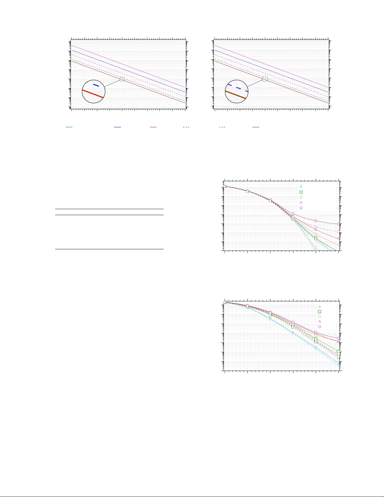
Comments & Academic Discussion
Loading comments...
Leave a Comment