Infinite-Dimensional Closed-Loop Inverse Kinematics for Soft Robots via Neural Operators

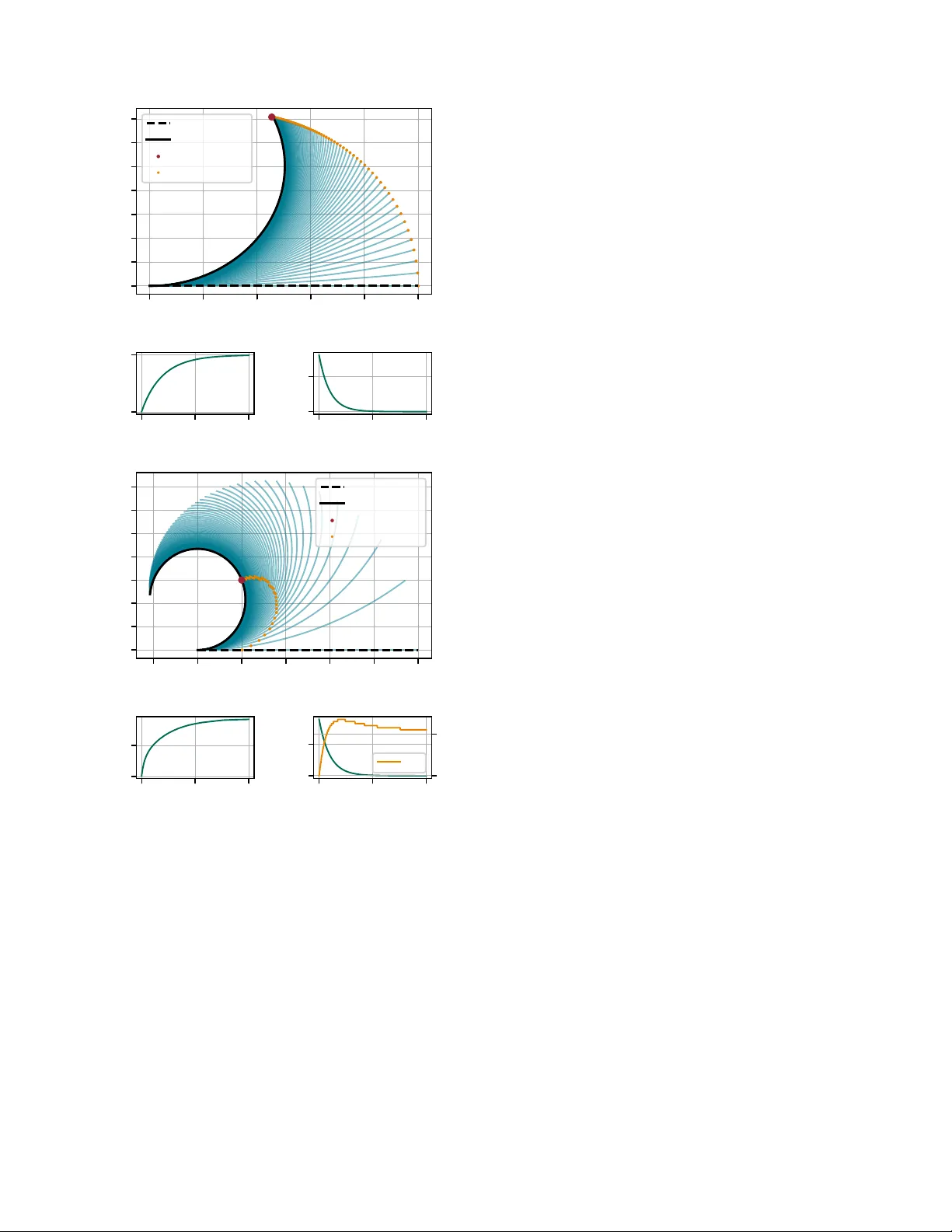
Infinite-Dimensional Closed-Loop In verse Kinematics f or Soft Robots via Neural Operators Carina V eil 1 , Moritz Flaschel 2 , Ellen Kuhl 1 , and Cosimo Della Santina 3 Abstract — While kinematic in version is a purely geometric problem f or fully actuated rigid robots, it becomes extremely challenging for underactuated soft r obots with infinitely many degrees of freedom. Closed-loop in verse kinematics (CLIK) schemes address this by intr oducing end-to-end mappings from actuation to task space for the controller to operate on, but typically assume finite dimensions of the underlying virtual configuration space. In this work, we extend CLIK to the infinite-dimensional domain to reason about the entire soft robot shape while solving tasks. W e do this by composing an actuation-to-shape map with a shape-to-task map, deriving the differential end-to-end kinematics via an infinite-dimensional chain rule, and thereby obtaining a Jacobian-based CLIK algorithm. Since the actuation-to-shape mapping is rarely av ailable in closed f orm, we propose to lear n it from simulation data using neural operator networks, which are differentiable. W e first present an analytical study on a constant-curvature segment, and then apply the neural version of the algorithm to a three-fiber soft robotic arm whose underlying model relies on morphoelasticity and active filament theory . This opens new possibilities for differentiable contr ol of soft r obots by exploiting full-body shape information in a continuous, infinite-dimensional framework. I . I N T RO D U C T I O N Kinematic in version refers to finding a feasible robot configuration such that the robot assumes a desired posi- tioning of one or more of its parts in space [1]. For a rigid manipulator , this usually translates to computing joint positions that result in a desired end-ef fector pose, given the geometric link parameters. This formulation, ho we ver , assumes full actuation of rigid robots. When the robot itself becomes soft and can bend and twist continuously rather than only at discrete joints, its nature-inspired flexibility opens ne w possibilities in navigating complex en vironments and interacting safely with delicate objects, yet this same property mak es control in general challenging and even the usually straightforward task of kinematic in version difficult. Related W ork. For fully actuated systems, where the degrees of actuation equal the degrees of freedom, kinematic in version is a purely geometric problem, in which desired This w ork w as supported by the NSF CMMI A ward 2318188 Mechanics of Bioinspired Soft Slender Actuators and the ERC Advanced Grant 101141626 DISCO VER. Corresponding author: Carina V eil. 1 C. V eil and E. Kuhl are with the Department of Mechan- ical Engineering, Stanford Uni versity , Stanford, CA 94305, USA. { cveil,ekuhl } @stanford.edu 2 M. Flaschel is with the Institute of Applied Mechanics, Friedrich- Alexander -Universit ¨ at Erlangen–N ¨ urnberg, 91058 Erlangen, German y . moritz.flaschel@fau.de 3 C. Della Santina is with the Cogniti ve Robotics Department, Delft Univ ersity of T echnology , 2628 Delft, The Netherlands. c.dellasantina@tudelft.nl joint configurations can be selected freely from the en- tire configuration space. Jacobian-based closed-loop in verse kinematics ( CLIK ) schemes e xploit this by using feedback in task-space to map back to required joint velocities via the Jacobian in verse, av oiding the need to solve the full nonlinear in verse kinematics problem at ev ery step [2]–[5]. Howe ver , in under-actuated systems with fewer degrees of actuation than degrees of freedom, such as soft robots, not all configurations are attainable through control action [6]. Static kinematic constraints must be enforced explicitly , typically via a numerical optimization, which is then embedded, for example, in a model predictiv e control fashion [7]–[10]. A compact, closed-loop form similar to the fully actuated case only becomes possible once we introduce an end-to-end kinematic mapping from the actuator inputs to the task-space output [11]: This mapping plays the role of a virtual joint- space model, like a controllable subspace, on which standard CLIK algorithms can then operate [12]–[16]. This so-called actuator-to-task closed-loop in verse kinematics approach was formalized for underactuated mechanical systems in [17], howe ver , still assuming finite dimensions for the underlying virtual joint space. i.e., relying on the common soft robot approximation that the shape is linearly parametrizable with a set of basis functions. But what if we want to reason on the entire (infinite-dimensional) soft robot shape while solving tasks? Contribution. In this work, we extend CLIK to systems with infinite-dimensional shape spaces, while keeping the controller finite-dimensional through end-to-end mappings from finite actuators to finite task dimensions. T o this end, we define two mappings: (i) the mapping from actuators to shape, that is, the “internal” model of the (soft) robot, (ii) the forward kinematics from an infinite-dimensional shape space to a task, whose composition yields the end-to-end forward kinematics from actuation to task. Combining the gradients of both mappings via an infinite-dimensional chain rule yields the end-to-end forward differential kinematics, and the standard Jacobian-based CLIK algorithm applies. It quickly becomes obvious that the key challenge here is that soft robots’ actuator-to-shape mappings are highly complex and often lack closed-form expressions or explicit Jacobians, so that the proposed CLIK algorithm is only practical with a learned , differentiable model of this map. T o adress this, we propose to learn the mapping from simulation data using a neural operator network , which, unlike traditional neu- ral networks, learns mappings between infinite-dimensional function spaces without fix ed discretization, while providing well-defined gradients with respect to the finite-dimensional Fig. 1: (Neural) Infinite-dimensional closed-loop inv erse kinematics (CLIK) : W e propose an extension of finite-dimensional CLIK that allows us to reason on the whole soft robot shape while solving tasks. Since analytical expressions of the Jacobian are difficult to obtain in practice for infinite-dimensional soft robot models, we embed a neural version of the algorithm that uses the neural operator of the robot learned from simulations. inputs [18], [19]. Neural operators are a recent trend in machine learning that hav e found wide interest in control and (soft) robotics already , for example as surrogate models for comple x dynamics and soft materials [20]–[24], or to make comple x or computationally expensi ve control schemes either real-time feasible or differentiable [25]–[29]. For us, they enable reasoning about the full infinite-dimensional soft robot shape during tasks. Organization. First, we re view finite-dimensional CLIK for underactuated mechanical systems in Section II, and then introduce its extension to infinite-dimensional shapes in Section III. Last but not least, Section IV presents the neural version of the algorithm. I I . P R E L I M I NA R I E S : ( F I N I T E - D I M E N S I O N A L ) C L O S E D - L O O P I N V E R S E K I N E M AT I C S Before introducing our extension to infinite-dimensional closed-loop inv erse kinematics, we will briefly re view the finite-dimensional case and unify notations. W e refer to [30] and [17] for extended clarifications. Kinematic inv ersion. Intuiti vely , forward kinematics an- swer “If I set the r obot joints to these angles, where does the tip end up?” , while kinematic in version solves the re verse: “Which joint angles will get my tip to the desired position?” Formally , let q ∈ R n be the configuration space of a mechan- ical system with n degrees of freedom. Further , let x ∈ R p be a p -dimensional task coordinate, commonly the end-effector position and orientation, such that the robot fulfilling the tasks is expressed through the forward kinematics Φ fin : R n → R p , q 7→ x = Φ fin ( q ) . (1) The goal of kinematic inv ersion is to, given a desired task coordinate ¯ x , find a configuration ¯ q such that ¯ x = Φ fin ( ¯ q ) . Closed-loop in verse kinematics (CLIK). This control scheme looks for solutions of the kinematic inv ersion in the form of dynamical system ˙ q = c IK ( q , ¯ x ) s.t. lim t →∞ Φ fin ( q ( t )) = ¯ x (2) so that its equilibrium ¯ q satisfies the kinematic in version ¯ x = Φ fin ( ¯ q ) . A standard choice for this dynamical system that ensures exponential con ver gence under mild assumptions is ˙ q = J Φ fin ( q ) − 1 K ( ¯ x − Φ fin ( q )) (3) with positi ve definite gain matrix K and associated Jacobian J Φ fin , which is square and inv ertible for the fully actuated case with p = n . It follows from linearizing the task error ˜ x = ¯ x − Φ fin ( q ) and requiring the closed-loop dynamics ˙ ˜ x = − K ˜ x in task space. In verting through the Jacobian yields (3), which exhibits exponential con vergence provided the Jacobian remains in vertible. CLIK f or underactuated systems. For underactuated systems with m < n , we cannot control the n -dimensional configuration space, but we can extend the above to finding a control c IK that also respects static constraints, i.e., ˙ q = c IK ( q , ¯ x ) s.t. lim t →∞ Φ fin ( q ( t )) = ¯ x and lim t →∞ q ( t ) ∈ E , (4) where E is the attainable equilibria set containing all con- figurations that can be reached as a steady state [17]. T o realize this, we hav e to introduce an end-to-end mapping from actuators to task output that creates a virtual configura- tion subspace controllable by actuators on which CLIK can operate. Therefore, consider the finite-dimensional mapping Λ fin : R m → R n , q a 7→ q , (5) from actuation coordinates q a with m independent degrees of actuation to configuration coordinates q , such that the composed forward pseudo-kinematics that maps actuators to task variables are (Φ ◦ Λ) fin : R m → R p , q a 7→ x = (Φ ◦ Λ) fin ( q a ) . (6) Note that, here, we focus on a square in version prob- lem where the actuation space and task space ha ve equal dimension ( m = p ), making the actuation-to-task map- ping non-redundant. The corresponding square Jacobian is J (Φ ◦ Λ) fin ( q a ) . Then, the standard gradient-based CLIK algo- rithm is ˙ q a =  J (Φ ◦ Λ) fin ( q a )  − 1 K ( ¯ x − (Φ ◦ Λ) fin ( q a )) . (7) where a positi ve definite gain matrix K ∈ R m × m ensures exponential con ver gence analogous to the fully actuated case. Fig. 2: Block diagram of the infinite-dimensional closed-loop in- verse kinematics (23) in actuation space q a ∈ R m , with a square actuation-to-task mapping. Trapezoids emphasize the change in dimensionality from input to output. I I I . I N FI N I T E - D I M E N S I O NA L C L O S E D - L O O P I N V E R S E K I N E M A T I C S For the infinite-dimensional analogue of (7), we introduce a general (soft) robot model via the actuation-to-shape mapping Λ : R m → X , q a 7→ r = Λ( q a ) , (8) where X = L 2 ([0 , 1]; R 3 ) is a Hilbert space of square- integrable curves with respect to the normalized spatial coordinate s ∈ [0 , 1] , and equipped with the standard L 2 - inner product. Furthermore, r : [0 , 1] → R 3 is a C 1 curve representing the soft robot shape in space 1 . Note that we parametrize attainable shapes by actuator coordinates q a ∈ R m , so the attainable-equilibria manifold forms an m - dimensional submanifold of the infinite-dimensional function space X . Next, let Φ denote a p -dimensional task, i.e. the shape-to-task mapping Φ : X → R p , r 7→ x = Φ( r ) . (9) such that the end-to-end mapping from actuation to task on which CLIK operates is the composition Φ ◦ Λ : R m → R p , q a 7→ x = (Φ ◦ Λ)( q a ) . (10) A. Differ ential Kinematics T o realize the infinite-dimensional CLIK version of (7), we need the end-to-end Jacobian J Φ ◦ Λ ( q a ) ∈ R p × m , which is obtained via the differentials of the component mappings Λ and Φ , connected by the chain rule. Actuation-to-shape. The Fr ´ echet deri v ativ e of Λ at q a , Λ ′ ( q a ) , is a bounded linear map Λ ′ ( q a ) : R m 7→ X , Λ( q a + δ q a ) = Λ( q a ) + Λ ′ ( q a )[ δ q a ] + o ( ∥ δ q a ∥ ) , (11) that maps small changes in actuators to small changes in shape. Since our actuation is finite dimensional, the Fr ´ echet deriv ativ e reduces to a linear combination of partial deriv a- tiv es in the function space, Λ ′ ( q a )[ δ q a ] = m X i =1 δ q a ,i ∂ Λ( q a ) ∂ q a ,i , (12) ∂ Λ( q a ) ∂ q a ,i =: ∂ q a ,i Λ( q a ) ∈ X . 1 Normalized arc-length s ∈ [0 , 1] is used without loss of generality via the standard reparameterization s = ˜ s/L . The formulation also holds in R 2 . Shape-to-task. For a perturbation v : [0 , L ] 7→ R 3 , define the perturbed shape r ε = r + εv and the directional deriv ati ve Φ ′ ( r )[ v ] = d dε Φ( r ε )   ε =0 . (13) The directional deri vati ve Φ ′ ( r )[ v ] defines a bounded linear functional on the tangent space of admissible perturbations v . Endo wing this space with a Hilbert structure (such as X = L 2 ([0 , 1]; R 3 ) ) with inner product ⟨ u, v ⟩ L 2 = Z 1 0 u ( z ) · v ( z ) dz, (14) the Riesz representation theorem [31] ensures the existence of a unique element ∇ X Φ( r ) ∈ X such that Φ ′ ( r )[ v ] = ⟨∇ X Φ( r ) , v ⟩ X , ∀ v ∈ X , (15) i.e. the L 2 gradient of Φ at r . End-to-end. For the CLIK algorithm, we consider the differential end-to-end kinematics ˙ x = J Φ ◦ Λ ( q a ) ˙ q a , J Φ ◦ Λ ∈ R p × m . (16) For an y direction ˙ q a ∈ R m , by chain rule, the deriv ativ e of this composition is (Φ ◦ Λ) ′ ( q a )[ ˙ q a ] =  Φ ′ ( r )  Λ ′ ( q a )[ ˙ q a ]  . (17) T ogether with the task differential Φ ′ ( r )[ v ] (15), this yields (Φ ◦ Λ) ′ ( q a )[ ˙ q a ] =  ∇ X Φ( r ) , Λ ′ ( q a )[ ˙ q a ]  X (18) =  Λ ′ ( q a ) ∗ ∇ X Φ( r ) , ˙ q a  R m , (19) where Λ ′ ( q a ) ∗ : X → R m is the Hilbert adjoint. Comparing this with the differential end-to-end kinematics (16), we note that the Jacobian of the composition must be J Φ ◦ Λ ( q a ) = Λ ′ ( q a ) ∗ ∇ X Φ(Λ( q a )) ∈ R p × m , (20) and its i -th column is calculated as J Φ ◦ Λ , : ,i ( q a ) = ⟨∇ X Φ(Λ( q a )) , ∂ q a ,i Λ( q a ) ⟩ X , (21) = Z L 0 ∂ q a ,i Λ( q a )( z ) · ∇ X Φ(Λ( q a ))( z ) dz (22) for i = 1 , 2 , .., m . When p = m and J Φ ◦ Λ ( q a ) is nonsingular , following the usual steps for kinematic in version yields the final CLIK algorithm (cf. Figure 2) ˙ q a = ( J Φ ◦ Λ ( q a )) − 1 K ( ¯ x − (Φ ◦ Λ)( q a )) , (23a) r = ¯ r ( q a ) (23b) with positiv e definite gain matrix K ∈ R m × m . Pr oposition 1: The closed-loop kinematic in version (23) solves (4) exponentially fast ∀ K ≻ 0 . Pr oof: First, we formulate the differential kinematics of the end-to-end mapping (16), and plug in the proposed controller (23) ˙ x = J Φ ◦ Λ ( q a ) ˙ q a (24) = J Φ ◦ Λ ( q a ) ( J Φ ◦ Λ ( q a )) − 1 K ( ¯ x − (Φ ◦ Λ)( q a )) (25) = K ( ¯ x − (Φ ◦ Λ)( q a )) . (26) W e observ e that the resulting error dynamics ˙ ¯ x − ˙ x = − K ( ¯ x − x ) is linear and con verges exponentially fast to zero with the rated defined by K . Consequently , the steady state Fig. 3: While standard tasks usually focus to position the end- effector r ( ¯ s = 1) , the continuum nature of the soft robot in vites for just reaching a target point with the closest point r ( s ∗ ) on its backbone, where s ∗ is adapted in each iteration. of (23) fulfills lim t →∞ Φ( q ( t )) = ¯ x . B. Repr esentative T asks and Resulting J acobians W e can think of many functionals Φ : X → R p in the task space of a robot. The most common examples in volv e reaching a target or a prescribed distance from it for a specific point along the robot’ s body , typically the end-ef fector for rigid robots. While such tasks are equally relev ant for soft robots, their continuous nature in vites an adaptation of this formulation: rather than requiring the end-effector to reach the target, we may instead define the task such that the point along the robot’ s body closest to the target reaches it (cf. Figure 3). Positioning tasks. Reaching a target point x 0 (or time- varying x 0 ( t ) ) at a fixed centerline coordinate ¯ s ∈ [0 , 1] (or ¯ s ( t ) ) of the robot centerline r translates to Φ fixed pos ( r ) = r ( ¯ s ) − x 0 . (27) Howe ver , our infinite-dimensional CLIK shines for the more expressi ve closest-point task, which automatically identifies the best location along the entire robot shape to reach the target. This is formulated as Φ opt pos ( r ) = r ( s ∗ ) − x 0 , (28a) where s ∗ = argmin s ∈ [0 , 1] 1 2 ∥ r ( s ) − x 0 ∥ 2 , (28b) meaning that the closest centerline coordinate s ∗ to the target is determined through optimization at each step. The L 2 -gradients of the positioning tasks are ∇ L 2 Φ fixed pos ( r ) = δ ( s − ¯ s ) ∈ X , and ∇ L 2 Φ opt pos ( r ) = δ ( s − s ∗ ) ∈ X , such that the Jacobians of the end-to-end mapping J Φ ◦ Λ ∈ R 3 × m hav e m columns J (Φ fixed pos ◦ Λ): ,i ( q a ) = ∂ q a ,i Λ( q a )( ¯ s ) , (29) J (Φ opt pos ◦ Λ): ,i ( q a ) = ∂ q a ,i Λ( q a )( s ∗ ) , (30) i.e., only the partial deri vati ve of the actuation-to-shape mapping at the respecti ve s -coordinate remains. Distance tasks. Scalar distance tasks follow the same structure. The fixed-coordinate variant minimizes squared distance from a prescribed centerline coordinate ¯ s ∈ [0 , 1] Φ fixed dist ( r ) = 1 2 ∥ r (¯ s ) − x 0 ∥ 2 . (31) Again, infinite-dimensional CLIK excels when minimizing the distance from the closest point on the centerline Φ opt dist ( r ) = min s ∈ [0 , 1] 1 2 ∥ r ( s ) − x 0 ∥ 2 , (32) where, the closest centerline coordinate s ∗ directly results from the distance optimization. Assuming uniqueness and nondegenerac y of the minimizer (Infinite-dimensional Dan- skin’ s Theorem, cf. Theorem 4.13 in [32]), its directional deriv ativ e follows (15) with L 2 -gradients ∇ L 2 Φ fixed dist ( r ) = ( r ( s ∗ ) − x 0 ) δ ( s − s ∗ ) ∈ X , and ∇ L 2 Φ opt dist ( r ) = ( r ( s ∗ ) − x 0 ) δ ( s − ¯ s ) ∈ X , such that the row Jacobians of the end-to- end mapping J Φ ◦ Λ ∈ R 1 × m hav e m scalar entries J (Φ fixed dist ◦ Λ) ,i ( q a ) =  ∂ q a ,i Λ( q a )( ¯ s )  ⊤ ( r (¯ s ) − x 0 ) , (33) J (Φ opt dist ◦ Λ) ,i ( q a ) =  ∂ q a ,i Λ( q a )( s ∗ )  ⊤ ( r ( s ∗ ) − x 0 ) . (34) C. T oy Example: Constant Curvatur e Se gment Let us no w consider an analytical example to demonstrate the infinite-dimensional CLIK algorithm. For the sake of simplicity , and almost w .l.o.g., assume a planar, inextensible robot such that the only strain is the curvature κ ( s ) , where s ∈ [0 , 1] is a normalized arc-length coordinate and the physical arc length is L . This leads to infinite-dimensional mapping Λ κ that maps curv ature functions to a backbone pose ( x, y , α ), more precisely , Λ κ ( κ )( s ) =   x ( s ) y ( s ) α ( s )   =   L R s 0 cos( α ( v )) dv L R s 0 sin( α ( v )) dv R s 0 κ ( v ) dv   . (35) Assuming a constant curvature q along the segment such that κ ( s ) ≈ q , and focusing on the centerline position r ( s ) = [ x ( s ) , y ( s )] without orientation, this simplifies to Λ CC ( q )( s ) = r ( s ) = " L sin( sq ) q L 1 − cos( sq ) q # (36) with Jacobian J CC ( q ) = L h sq cos( sq ) − sin( sq ) q 2 (cos( sq ) − 1)+ sq sin( sq ) q 2 i ⊤ . (37) Since the constant curv ature segment has only one degree of actuation, namely this curvature itself, i.e. q a = q , we require a one dimensional task such as the scalar distance task Φ fixed dist . The scalar Jacobian of the composition is then J Φ fixed dist ◦ Λ CC ( q ) = J CC ( q )( ¯ s )( r (¯ s ) − x 0 ) . (38) Reaching a point translates to eliminating the distance, i.e. ¯ x = Φ fixed dist ( ¯ r ) = 0 , such that the CLIK control is ˙ q = − K h J (Φ fixed dist ◦ Λ CC ) ( q ) i − 1 Φ fixed dist (Λ CC ( q )) (39) with scalar weight K > 0 . The same holds for the closest- point version of the task Φ opt dist with s ∗ instead of ¯ s . Figure 4 shows simulations of such a constant curvature segment reaching a tar get point at a fixed backbone coordi- 0 . 0 0 . 2 0 . 4 0 . 6 0 . 8 1 . 0 x 0 . 0 0 . 1 0 . 2 0 . 3 0 . 4 0 . 5 0 . 6 0 . 7 y P ositioning the tip Initial Final T arget P oint ¯ s 0 . 0 0 . 5 1 . 0 time 0 2 curv ature q 0 . 0 0 . 5 1 . 0 time 0 . 00 0 . 25 task x − 0 . 2 0 . 0 0 . 2 0 . 4 0 . 6 0 . 8 1 . 0 x 0 . 0 0 . 1 0 . 2 0 . 3 0 . 4 0 . 5 0 . 6 0 . 7 y P ositioning the closest-point Initial Final T arget P oint s ∗ 0 . 0 0 . 5 1 . 0 time 0 . 0 2 . 5 curv ature q 0 . 0 0 . 5 1 . 0 time 0 . 000 0 . 025 task x s ∗ 20 40 Fig. 4: Constant curvature segment: Robot ev olution and time ev olutions ( t ∈ [0 , 1] ) of the actuation v ariable q and the task variable x for the point-reaching task Φ fixed pos (top) and the closest- point task Φ fixed opt (bottom). nate (the tip position in this case), as well as the closest-point task where any point on the robot should reach the target as fast as possible. In both scenarios, the scalar weight is K = 10 and we observe exponential con ver gence. For the closest-point task, the optimal coordinate s ∗ is continuously updated to the point nearest to the tar get. I V . N E U R A L C L O S E D - L O O P I N V E R S E K I N E M A T I C S While the previous e xample demonstrates how the infinite- dimensional CLIK works and what possibilities we hav e when being able to reason on the whole soft body shape while solving tasks, we recognize that the first of the two maps Λ is very hard to obtain in closed form in practice, especially once more complex soft robots are inv olved. This is why we propose to learn the soft robot model operator of the actuation-to-shape mapping Λ (8), denoted as G Λ , via neural operator networks . A. Neural Operator Networks and Their Gr adients The universal operator theorem [33] shows that a neural network with one hidden layer can approximate any con- tinuous nonlinear operators. Extending this, the DeepONet [19] architecture allo ws for learning operators of the form G : u 7→ G ( u ) , where both u and G ( u ) are functions defined on (infinite-dimensional) spaces. For any point s in the domain of G ( u ) , the value G ( u )( s ) is a real-valued v ector in R d . T o learn said operator, DeepONet takes as inputs the sampled v alues [ u ( x 1 ) , u ( x 2 ) , ..., u ( x m )] at a finite number of fixed locations x 1 , x 2 , ..., x m , together with the ev aluation points s . The architecture consists of two sub-networks, the branch network processing the input function, and the trunk network processing the e valuations points, G branch : R m → R v × d , u 7→ a br , G trunk : R → R v × d , s 7→ a tr , (40) where v is a hyperparameter controlling the width of the latent representation. The final prediction is computed as the inner product of the outputs of the branch and trunk netw orks ov er the latent dimension G ( u )( s ) = a br ⊙ a tr , (41) where ⊙ denotes the element-wise multiplication over the latent dimension. Once trained, the DeepONet realization is a dif ferentiable mapping with respect to all its inputs, so gradients with respect to both the input function samples and the e valuation coordinate s are obtained directly by automatic differentiation. In practice, the branch network is trained on finitely many function samples, while at inference time the trunk network can be e valuated ar arbitrarily many , arbitrarily fine locations s . This decouples the discretization of the input function from the resolution of the output, which is a ke y advantage of neural operators over discretization-based neural networks, and makes it particularly powerful for infinite-dimensional CLIK where we want to reason ov er the continuous robot shape and might be interested in finer discretizations. B. Example: Three-fiber Soft Robotic Arm T o demonstrate our neural infinite-dimensional CLIK al- gorithm, we consider a soft robotic arm initially designed with three liquid crystal elastomer fibers, inspired by the elephant trunk musculature. It is depicted in Figure 5. By design, this structure is soft and slender, and can grow , shrink, or actively remodel its intrinsic shape while also deforming elastically – which is why it is modelled as an ac- tive, morphoelastic filament [34], [35]. This model has been previously v alidated in experiments [36], [37], successfully used for path-planning algorithms [38], and shall no w serve as e xample for the neural operator implementation of infinite- dimensional CLIK. W e briefly summarize this model here, but refer to [35], [37] for details. Fig. 5: Three-fiber soft robotic arm [36], [37]: The orientation of the fibers is inspired by the muscular structure of the elephant trunk, with one straight fiber and a helical fiber pair , enabling continuous deformations and optimal reachability . Morphoelasticity . Consider a tubular body of length L , which is reduced to the centerline r : [0 , 1] → R 3 with normalized spatial coordinate s ∈ [0 , 1] , and an orthonormal director frame D = { d 1 , d 2 , d 3 } , where d i : [0 , L ] → R 3 , is attached to r ( s ) for all s . The kinematics of the one- dimensional filament follow as r ′ ( s ) = ζ d 3 , (42a) d ′ i ( z ) = ζ u × d i , i = { 1 , 2 , 3 } , (42b) with the axial e xtension of the filament ζ and the Darboux curvature vector u = u 1 d 1 + u 2 d 2 + u 3 d 3 describing the ev olution of the director basis D along the filament. With- out external load, we refer to these properties as intrinsic curvatures u = ˆ u and intrinsic extension ζ = ˆ ζ . Under (gravitational) load, intrinsic and actual properties differ , and we further need to consider the quasi-static solution of the force and moment balance equations, namely ∂ n ∂ s + ˆ ζ f = 0 , ∂ m ∂ s + ∂ r ∂ s × n + ˆ ζ l = 0 . (43) Here, n is the internal force, ˆ ζ f is the external body force per unit length, m is the internal momentum, and ˆ ζ l is the external body couple per unit length. Active filaments. T o connect the filament model to the robot’ s actuation, we treat the soft robot as an active fil- ament whose material can locally shorten or extend along embedded fibers. The internal fiber architecture is described by a fiber direction field inside the filament body , which may be uniaxial or helical, and the corresponding intrinsic properties are obtained by integrating the fiber contributions ov er the cross section. While the proposed approach allo ws for general forms of activation γ i , in this work we consider piecewise uniform acti vations and obtain a single scalar v alue γ i ∈ R per fiber . W e identify these activ ation scalars with the actuation coordinates and write q a ,i := γ i , so that the actuation coordinate directly scales the intrinsic contraction of extension generated by each fiber . Negati ve activ ation γ i < 0 (or q a ,i < 0 ) corresponds to contraction , positiv e activ ation γ i > 0 (or q a ,i > 0 ) corresponds to extension . Three-fiber soft r obotic arm. The soft robot considered in this work has one longitudinal and two helical fibers inspired by the elephant trunk musculature (Figure 5) and is subject to gravitational load. Combining the above, its forward kinematics are go verned by r ′ ( s ) = ζ d 3 , (44a) d ′ i ( s ) = ˆ ζ u × d i , i = { 1 , 2 , 3 } , (44b) 0 = ∂ n ∂ s + ˆ ζ f (44c) 0 = ∂ m ∂ s + ∂ r ∂ s × n + ˆ ζ l . (44d) where the mapping from actuation q a ∈ R 3 to shape r ( s ) is mediated by the intrinsic curvature ˆ u and extension ˆ ζ , both of which are functions of the fiber activ ations, hence, the actuation, i.e., ˆ u ( q a ) and ˆ ζ ( q a ) . C. Learning the Model with a Neural Operator In our application, the architecture of the operator network is simplified compared to the DeepONet architecture [19], since the input is a single scalar-v alued actuation function and the actuation coordinates q a ∈ R m are already finite- dimensional. Consequently , the branch net reduces to a standard feedforward network that takes q a as input, while the trunk net only encodes the spatial variable s . At the same time, we retain the key property that the operator is learned ov er actuation and space, so we can ev aluate the learned actuation-to-shape mapping G Λ at arbitrarily man y points s and differentiate with respect to q a , which is exactly what the neural CLIK algorithm requires. Data. For data generation, we solve the boundary value problem (44) N = 1 , 000 , 000 times to obtain samples of the actuation-to-shape mapping for random activ ations within the physical constraints of the system q a ,i ∈ [ − 1 . 67 , 0] , i = 1 , 2 , 3 . Note that q a = 0 corresponds to the steady state of the system in which the soft robot hangs downw ard, and negati ve actuation leads to fiber contraction relative to this state. Histograms of the activ ations show that the entire actuation space is sufficiently represented in the dataset. The spatial coordinate s is discretized with n s = 100 points in [0 , 1] . W e use the J ulia package de veloped for the active filament theory [35] and the associated parameters of the minimal three fiber prototype [36]. W e store each solution as a discrete centerline in a matrix R ∈ R n s × 3 with its respectiv e ( x, y , z ) -coordinates at the n s locations. T raining process. Of the 1,000,000 samples, 200,000 are held out as a test set. From the remaining data, 640,000 samples are used for training and 160,000 for validation. W e train the operator network for 500 epochs with the Adam optimizer , tanh activ ations, batch size 32, and an exponentially decaying learning rate, using the validation loss to select the best model checkpoint (typically reached after 400-450 epochs). On the held-out test set, the trained − 0 . 050 − 0 . 025 0 . 000 0 . 025 x 0 . 000 0 . 025 0 . 050 y 0 . 000 0 . 025 0 . 050 0 . 075 P ositioning a fixed point Initial Final T arget ¯ s 0 . 0 0 . 5 1 . 0 time − 0 . 50 − 0 . 25 0 . 00 activ ations 0 . 0 0 . 5 1 . 0 time − 0 . 05 0 . 00 task γ 1 γ 2 γ 3 x y z − 0 . 025 0 . 000 0 . 025 0 . 050 x − 0 . 025 0 . 000 0 . 025 0 . 050 y 0 . 000 0 . 025 0 . 050 0 . 075 P ositioning the closest-point Initial Final T arget s ∗ 0 . 0 0 . 5 1 . 0 time − 0 . 4 − 0 . 2 0 . 0 activ ations 0 . 0 0 . 5 1 . 0 time − 0 . 01 0 . 00 task γ 1 γ 2 γ 3 x y z Fig. 6: Three-fiber soft robotic arm. Robot ev olution ( ) and time evolutions of the actuation variable ( activations γ i ) and the task variable x for the fixed point-reaching task Φ fixed pos (left) closest-point task Φ opt pos (right). For the robot ev olution, we plot ev ery 10th shape. model achiev es a mean squared error of 1 . 38 × 10 − 10 and an L 2 relativ e error of 6 . 08 × 10 − 4 . The architecture and test performance are summarized in T able I. Architectur e and T raining Optimizer Adam Activ ation tanh Learning rate Exponential decay Epochs 500 Batch size 32 Branch layers [3, 64, 64, 64, 192] T runk layers [1, 64, 64, 64, 192] T est Performance MSE 1 . 38 × 10 − 10 L2 relative error 6 . 08 × 10 − 4 T ABLE I: Neural operator hyperparameters and performance. D. Composed Jacobian and Neural CLIK The soft robot has three actuators, hence, we consider the three-dimensional tasks Φ fixed pos and Φ opt pos that position the robot with respect to a target point in ( x, y , z ) coordinates. From automatic differentiation, we obtain the gradient of the operator network G Λ with respect to the input q a . W ith the task gradients being Dirac at ¯ s or s ∗ , the Jacobian of the composition is the e valuation of the operator netw ork gradient at the required spatial coordinate ¯ s or s ∗ according to (29), (30), namely J Φ fixed pos ◦G Λ ( q a ) = ∂ G Λ ( q a ) ∂ q a ( ¯ s ) ∈ R 3 × 3 , (45) J Φ opt pos ◦G Λ ( q a ) = ∂ G Λ ( q a ) ∂ q a ( s ∗ ) ∈ R 3 × 3 . (46) Reaching a point translates to a desired task v ariable ¯ x = Φ pos ( ¯ r ) = [0 , 0 , 0] , and the control law follows as (23). Figure 6 sho ws simulations of the neural version of the infinite-dimensional CLIK algorithm for the two distinct positioning tasks. The simulation is for t ∈ [0 , 1] with a time step of dt = 0 . 001 . The weighting matrix is K = 8 · diag (1 , 1 , 1) , i.e., all positioning coordinates are equally weighted, and the magnitude is a balance between conv er- gence speed and ov ershooting. W e use a spatial discretization with n s = 100 points in this example, b ut this discretization could be arbitrarily finer . The code will be made available on GitHub upon acceptance. V . C O N C L U S I O N In this paper we extend classical closed-loop in verse kinematics (CLIK) to the infinite-dimensional shape space of soft robots, enabling controllers to reason directly on the entire robot shape while solving tasks. By composing an actuation-to-shape map with a shape-to-task map and applying an infinite-dimensional chain rule, we deriv e the corresponding dif ferential end-to-end kinematics and obtain a Jacobian-based CLIK algorithm. Since the actuation-to- shape mapping typically lacks closed-form expressions, we show how to learn it from simulation data using differentiable neural operator networks. The simulations focus on simple positioning tasks, yet the framework naturally extends to more comple x objecti ve functionals, and future work will explore how to incorporate obstacles or task-space trajectory tracking. Experimental v alidation is necessary to assess how the algorithm performs under model mismatch between the simulated (learned) operator and the real robot. R E F E R E N C E S [1] P . Larochelle and J. M. McCarthy , “Inv erse kinematics, ” in Encyclope- dia of Robotics , M. H. Ang, O. Khatib, and B. Siciliano, Eds. Berlin, Heidelberg: Springer Berlin Heidelberg, 2020, pp. 1–4. [2] C. Schumacher, E. Knoop, and M. B ¨ acher , “ A versatile inv erse kine- matics formulation for retargeting motions onto robots with kinematic loops, ” IEEE Robotics and Automation Letters , vol. 6, no. 2, pp. 943– 950, 2021. [3] M. D. Fiore and C. Natale, “On the con vergence of a closed-loop in verse kinematics solver with time-varying task functions, ” IEEE Robotics and Automation Letters , vol. 9, no. 1, pp. 81–86, 2023. [4] B. Kenwright, “Real-time character in verse kinematics using the gauss-seidel iterativ e approximation method, ” arXiv preprint arXiv:2211.00330 , 2022. [5] J. Colan, A. Davila, and Y . Hasegawa, “V ariable step sizes for iterativ e Jacobian-based inv erse kinematics of robotic manipulators, ” IEEE access , vol. 12, pp. 87 909–87 922, 2024. [6] I. Fantoni and R. Lozano, Non-Linear Contr ol for Underactuated Mechanical Systems . Springer Science & Business Media, 2012. [7] Y . W ang, Y . Liu, M. Leibold, M. Buss, and J. Lee, “Hierarchical incremental MPC for redundant robots: A robust and singularity-free approach, ” IEEE T ransactions on Robotics , vol. 40, pp. 2128–2148, 2024. [8] C. Duriez, E. Coevoet, F . Largilliere, T . Morales-Bieze, Z. Zhang, M. Sanz-Lopez, B. Carrez, D. Marchal, O. Goury , and J. Dequidt, “Framew ork for online simulation of soft robots with optimization- based in verse model, ” in 2016 IEEE International Confer ence on Simulation, Modeling, and Progr amming for Autonomous Robots (SIMP AR) . IEEE, 2016, pp. 111–118. [9] S. T onkens, J. Lorenzetti, and M. Pavone, “Soft robot optimal control via reduced order finite element models, ” in 2021 IEEE International Confer ence on Robotics and Automation (ICRA) . IEEE, 2021, pp. 12 010–12 016. [10] T . V otroubek and T . Kroupa, “Globally optimal inv erse kinematics as a quadratic program, ” arXiv pr eprint arXiv:2312.15569 , 2023. [11] R. J. W ebster III and B. A. Jones, “Design and kinematic modeling of constant curvature continuum robots: A revie w , ” The International Journal of Robotics Research , vol. 29, no. 13, pp. 1661–1683, 2010. [12] T . George Thuruthel, Y . Ansari, E. Falotico, and C. Laschi, “Control strategies for soft robotic manipulators: A survey , ” Soft r obotics , vol. 5, no. 2, pp. 149–163, 2018. [13] F . Campisano, S. Cal ´ o, A. A. Remirez, J. H. Chandler , K. L. Obstein, R. J. W ebster III, and P . V aldastri, “Closed-loop control of soft con- tinuum manipulators under tip follower actuation, ” The International journal of r obotics r esearc h , vol. 40, no. 6-7, pp. 923–938, 2021. [14] G. Fang, Y . T ian, Z.-X. Y ang, J. M. Geraedts, and C. C. W ang, “Efficient Jacobian-based in verse kinematics with sim-to-real transfer of soft robots by learning, ” IEEE/ASME T ransactions on Mechatr onics , vol. 27, no. 6, pp. 5296–5306, 2022. [15] J. M. Bern and D. Rus, “Soft IK with stif fness control, ” in 2021 IEEE 4th International Confer ence on Soft Robotics (RoboSoft) . IEEE, 2021, pp. 465–471. [16] J. Rogatinsky , D. Recco, J. Feichtmeier , Y . Kang, N. Kneier , P . Ham- mer , E. O’Leary , D. Mah, D. Hoganson, N. V . V asilyev et al. , “ A multifunctional soft robot for cardiac interv entions, ” Science Advances , vol. 9, no. 43, p. eadi5559, 2023. [17] C. Della Santina, “Pushing the boundaries of actuators-to-task kine- matic inv ersion: From fully actuated to underactuated (soft) robots, ” Author ea Pr eprints , 2025. [18] A. Anandkumar, K. Azizzadenesheli, K. Bhattacharya, N. K ov achki, Z. Li, B. Liu, and A. Stuart, “Neural operator: Graph kernel network for partial differential equations, ” in ICLR 2020 W orkshop on Integr a- tion of Deep Neural Models and Differ ential Equations , 2020. [19] L. Lu, P . Jin, G. Pang, Z. Zhang, and G. E. Karniadakis, “Learning nonlinear operators via DeepONet based on the universal approxima- tion theorem of operators, ” Natur e Machine Intelligence , vol. 3, no. 3, pp. 218–229, 2021. [20] G. M. Campbell, G. Muhaxheri, L. F . Guilhoto, C. D. Santangelo, P . Perdikaris, J. Pikul, and M. Y im, “ Activ e Learning Design: Model- ing Force Output for Axisymmetric Soft Pneumatic Actuators, ” Apr . 2025. [21] J. Gao, M. Y . Michelis, A. Spielberg, and R. K. Katzschmann, “Sim-to- Real of Soft Robots W ith Learned Residual Physics, ” IEEE Robotics and Automation Letters , vol. 9, no. 10, pp. 8523–8530, Oct. 2024. [22] L. Lingsch, M. Y . Michelis, E. de Bezenac, S. M. Perera, R. K. Katzschmann, and S. Mishra, “Beyond regular grids: Fourier-based neural operators on arbitrary domains, ” 2024. [23] P . Ma, P . Y . Chen, B. Deng, J. B. T enenbaum, T . Du, C. Gan, and W . Matusik, “Learning neural constituti ve laws from motion observ a- tions for generalizable pde dynamics, ” in International Confer ence on Machine Learning . PMLR, 2023, pp. 23 279–23 300. [24] L. Chen, G. Chen, X. Liu, J. Su, X. L yu, L. W ang, and Y . Li, “Shape- morphing programming of soft materials on complex geometries via neural operator, ” arXiv preprint , 2026. [25] L. Bhan, Y . Shi, and M. Krstic, “Neural operators for bypassing gain and control computations in PDE backstepping, ” IEEE T ransactions on Automatic Contr ol , vol. 69, no. 8, pp. 5310–5325, 2023. [26] V . Kumar , S. Goswami, K. K ontolati, M. D. Shields, and G. E. Kar- niadakis, “Synergistic learning with multi-task DeepONet for efficient PDE problem solving, ” Aug. 2024. [27] M. Lamarque, L. Bhan, Y . Shi, and M. Krstic, “ Adaptiv e neural- operator backstepping control of a benchmark hyperbolic PDE, ” Automatica , vol. 177, p. 112329, 2025. [28] T . O. de Jong, K. Shukla, and M. Lazar , “Deep operator neural netw ork model predictive control, ” arXiv pr eprint arXiv:2505.18008 , 2025. [29] J. Hu, J. Qi, and J. Zhang, “Neural operator based reinforcement learning for control of first-order PDEs with spatially-varying state delay , ” 2025. [30] B. Siciliano, “ A closed-loop inverse kinematic scheme for on-line joint-based robot control, ” Robotica , vol. 8, no. 3, pp. 231–243, 1990. [31] J. Neuberger, Sobolev Gradients and Differential Equations . Springer Science & Business Media, 2009. [32] J. F . Bonnans and A. Shapiro, P erturbation Analysis of Optimization Pr oblems . Springer Science & Business Media, 2013. [33] T . Chen and H. Chen, “Universal approximation to nonlinear operators by neural networks with arbitrary activation functions and its applica- tion to dynamical systems, ” IEEE T ransactions on Neural Networks , vol. 6, no. 4, pp. 911–917, 1995. [34] D. E. Moulton, T . H. Lessinnes, and A. Goriely , “Morphoelastic rods. Part I: A single growing elastic rod, ” J ournal of the Mechanics and Physics of Solids , vol. 61, no. 2, pp. 398–427, 2013. [35] B. Kaczmarski, D. E. Moulton, E. Kuhl, and A. Goriely , “ Active fila- ments I: Curvature and torsion generation, ” Journal of the Mechanics and Physics of Solids , vol. 164, p. 104918, 2022. [36] S. Leanza, J. Lu-Y ang, B. Kaczmarski, S. W u, E. K uhl, and R. R. Zhao, “Elephant trunk inspired multimodal deformations and movements of soft robotic arms, ” Advanced Functional Materials , vol. 34, no. 29, p. 2400396, 2024. [37] B. Kaczmarski, S. Leanza, R. Zhao, E. K uhl, D. E. Moulton, and A. Goriely , “Minimal design of the elephant trunk as an active Filament, ” Physical Review Letters , vol. 132, no. 24, p. 248402, Jun. 2024. [38] C. V eil, M. Flaschel, and E. K uhl, “Shape-space graphs: Fast and collision-free path planning for soft robots, ” arXiv preprint arXiv:2510.03547 , 2025.