Field imaging framework for morphological characterization of aggregates with computer vision: Algorithms and applications

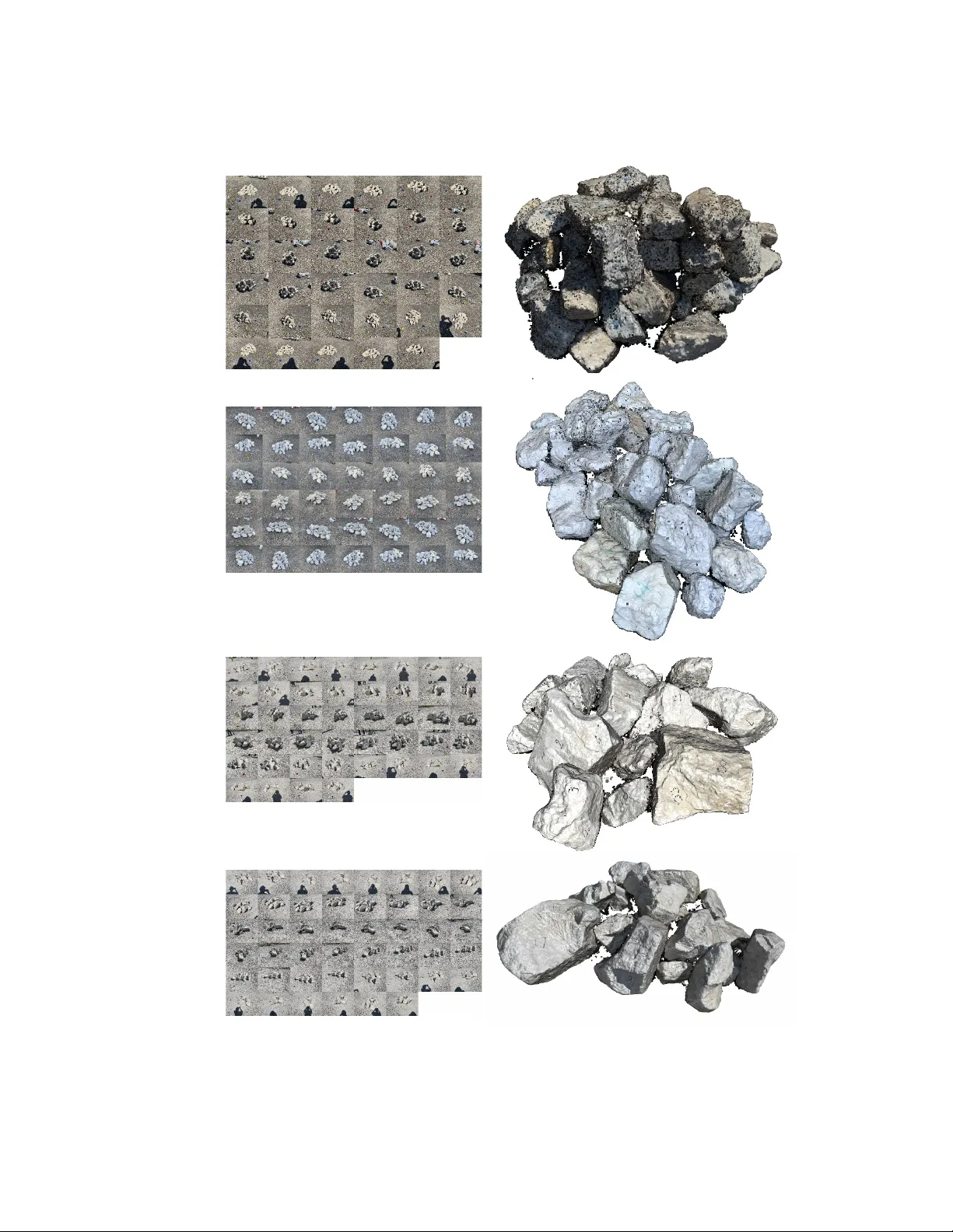
© 2021 Haohang Huang FIELD IMA GING FRAMEW ORK F OR MORPHOLOGICAL CHARA CTERIZA TION OF A GGREGA TES WITH COMPUTER VISION: ALGORITHMS AND APPLICA TIONS BY HA OHANG HUANG DISSER T A TION Submitted in partial fulﬁllmen t of the requiremen ts for the degree of Do ctor of Philosoph y in Civil Engineering in the Graduate College of the Univ ersit y of Illinois Urbana-Champaign, 2021 Urbana, Illinois Do ctoral Committee: Professor Erol T utumluer, Chair and Director of Researc h Professor Imad Al-Qadi Professor Jeﬀery R. Ro esler Asso ciate Professor Mani Golparv ar-F ard Professor Sanja y P atel ABSTRA CT Construction aggregates, including sand and gra v el, crushed stone and riprap, are the core building blo c ks of the construction industry , national economy , and so ciety . In the y ear 2020, in total 2.42 billion metric tons of aggregates v alued at $ 27.0 billion were pro duced b y ab out 5,400 mining companies op erating more than 10,000 quarries across all 50 states. Through mining, quarrying, and m ulti-lev el crushing and screening pro cesses, aggregates pro duced in diﬀeren t sizes and forms constitute the main skeleton of civil infrastructure and are extensively used in structural, transp ortation, geotec hnical, and hydraulic engineering applications. A t b oth quarry pro duction lines and construction sites, the morphological prop erties of aggregates (such as size, shap e, volume/w eight, etc.) are some of the most crucial indicators for aggregate Qualit y Assurance and Qualit y Con trol (QA/QC), esp ecially for crushed ag- gregates and riprap. State-of-the-practice metho ds mainly use sieving and caliper devices for the size and shap e determination of the most commonly used regular sizes of crushed aggre- gates, and are limited to visual inspection and man ual measuremen t for relatively large-sized aggregates. As a more adv anced quantitativ e approach, state-of-the-art aggregate imaging metho ds dev elop ed to date fo cus on characterizing aggregate morphology from acquired im- age data and mac hine vision analysis, y et with the limitation that most systems are only applicable to regular-sized aggregates under w ell-con trolled lab oratory conditions. The state-of-the-practice and state-of-the-art metho ds ha ve encountered several ma jor c hallenges in c haracterizing aggregate morphology . First, quantitativ e methods for capturing and analyzing aggregates are required to provide reliable c haracterization of the material. Second, ﬂexible and eﬀective metho ds are urgently needed for relatively large-sized aggre- gates. F urthermore, adv anced analyses are necessary to handle the most practical form of aggregate presence, such as densely stac k ed aggregates in sto ckpiles and/or in constructed la y ers. Lastly , three-dimensional (3D) imaging approaches are deemed ideal by pro viding more comprehensiv e and realistic aggregate information than tw o-dimensional (2D) image analyses. This dissertation presen ts the researc h eﬀort to address these ma jor c hallenges b y dev eloping a ﬁeld imaging framework for the morphological c haracterization of aggregates as a m ulti-scenario solution. The framew ork also has a focus on relativ ely large-sized aggregates, for whic h eﬀectiv e and eﬃcien t ﬁeld c haracterization metho ds are extremely lac king. F or individual and non-o v erlapping aggregates, a ﬁeld imaging system was designed ﬁrst, and the asso ciated image segmen tation and v olume estimation algorithms w ere devel- ii op ed. The color-based image segmen tation algorithm pro vides robust ob ject extraction under v arious ﬁeld lighting conditions suc h as strong sunlight and shado wing, and the v olumet- ric reconstruction algorithm estimates the particle v olume b y orthogonal in tersection. The approac h demonstrated go o d agreemen ts with ground-truth measurements made at quarry sites and achiev ed great impro vemen ts in the v olumetric estimation of individual aggregates when compared with the state-of-the-practice insp ection metho ds. F or 2D image analyses of aggregates in sto c kpiles, an automated 2D instance seg- men tation and morphological analysis approach was established based on deep learning. A task-sp eciﬁc sto c kpile aggregate image dataset was compiled based on images collected from aggregate pro ducers and individual aggregates in the images were manually lab eled to provide the ground-truth for learning. A state-of-the-art ob ject detection and segmen- tation arc hitecture w as implemen ted to train the image segmen tation kernel for sto ckpile segmen tation. The segmen tation results sho wed go o d agreement with ground-truth lab el- ing and pro vided eﬃcien t morphological analyses on images containing densely stac ked and o v erlapping aggregates. F or 3D p oint cloud analyses of aggregates in sto ckpiles, an end-to-end, in tegrated 3D Reconstruction-Segmen tation-Completion (RSC-3D) approac h w as established b y collab o- rating three dev elop ed comp onents, i.e., laboratory and ﬁeld 3D reconstruction procedures, 3D sto ckpile instance segmen tation, and 3D shape completion. The approach w as designed to reconstruct aggregate sto c kpiles from m ulti-view images, segment the stockpile into indi- vidual instances, and predict the unseen side of each instance based on the partial visible shap es. First, a 3D reconstruction pro cedure was dev elop ed to obtain high-ﬁdelit y full 3D mo dels of collected aggregate samples, based on which a 3D aggregate particle library w as constructed, and a comparativ e analysis w as conducted regarding the 2D and 3D morpho- logical c haracteristics. Next, t w o datasets were prepared based on the 3D particle library for 3D learning purp ose: (i) a synthetic dataset of aggregate sto ckpiles with ground-truth instance lab els dev elop ed with a synthetic data generation pipeline in volving mo del fabri- cation, sto ckpile assembly , and sto ckpile raycasting; and (ii) a dataset of partial-complete shap e pairs, developed with v arying-visibilit y and v arying-view raycasting sc hemes. Based on the t w o datasets, a state-of-the-art 3D instance segmentation netw ork and a 3D shap e completion net work w ere implemen ted and trained, resp ectiv ely . The application of the in te- grated approac h was demonstrated on re-engineered sto c kpiles and ﬁeld sto ckpiles, and the v alidation results against ground-truth measuremen ts sho wed go o d p erformance in capturing and predicting the unseen sides of aggregates, esp ecially in terms of size dimension metrics. In summary , the dev elop ed ﬁeld imaging framew ork in this study encompasses three ma jor approaches that characterize v arious forms and represen tations of ﬁeld aggregates iii with increasing analysis complexit y: (i) a volumetric reconstruction approac h for individual and non-ov erlapping aggregates; (ii) a 2D instance segmentation and morphological analysis approac h for aggregates in sto c kpiles based on 2D image analysis; and (iii) a 3D in tegrated reconstruction-segmen tation-completion approac h for aggregates in sto c kpiles based on 3D p oin t cloud analysis. The framew ork addresses the ma jor c hallenges of c haracterizing indi- vidual aggregates and aggregate sto ckpiles in the ﬁeld, thus provides a m ulti-scenario solution for eﬃcien t 2D and 3D analyses of aggregates. iv T o my p ar ents Gang Huang and Xiaoxia Liu, my sister Shuyan Liu, and my love Yihui Li. v A CKNO WLEDGMENTS First of all, I am deeply indebted to m y men tor and advisor, Professor Erol T utumluer, for his constant supp ort, insigh tful guidance, and inspiring though ts throughout this doctoral researc h. I am fortunate to b e nurtured by suc h a understanding, patien t, and hum ble advisor, without whom an y step of this work w ould not hav e b een p ossible o v er the y ears. He devoted his passion and kindness to the studen ts and b onded the research group as a heart-w arming family with his fatherly advice. The metho dology and philosoph y I learned from him hav e greatly shap ed my mindset of critical thinking and problem solving. His w ords and trust ha v e given me unlo ck ed p ow ers far b eyond kno wledge and education, which I know surely , remem b ered and enshrined, are m y constant companions and comforters in life. I w ould also lik e to extend my deep est appreciation to my other do ctoral committee mem b ers: Professor Imad Al-Qadi, Professor Jeﬀery R. Ro esler, Professor Mani Golparv ar- F ard, and Professor Sanja y Patel, for their inno v ative ideas, insightful commen ts, and join t con tribution to w ards improving this research. Professor Imad Al-Qadi and Professor Jeﬀery R. Roesler ha v e shared coun tless ideas that greatly impro v e this research to address practical engineering c hallenges, and the Adv anced T ransp ortation Researc h and Engineering Lab ora- tory (A TREL) facilit y they manage serv ed as the foundation of every activity conducted in this researc h. I am also very grateful to Professor Mani Golparv ar-F ard and Professor Sanjay P atel, who hav e b een unreservedly oﬀering m ulti-disciplinary views from computer science and electrical engineering and encouraging me to bring the cutting-edge technology in to m y researc h. All do ctoral committee mem b ers, with their hard-w orking attitude, w ell-rounded kno wledge, and leadership skills, are the role mo dels for m y future professional developmen t. I w ould like to thank all researc h partners and pro ject sp onsors who ha ve b een inv olved directly or indirectly in the success of this research. The research w as mainly supported b y ICT-R27-182 and ICT-R27-214 pro jects, whic h were conducted in co op eration with the Illinois Center for T ransp ortation (ICT); the Illinois Department of T ransp ortation (IDOT); and the U.S. Department of T ransp ortation, F ederal Highw ay Administration. The research w as conducted as an interdisciplinary collab oration eﬀort with Professor Narendra Ah uja from Electrical and Computer Engineering (ECE) department and John M. Hart, principal researc h engineer at the Computer Vision and Rob otics Lab oratory (CVRL). I very m uc h appreciate the unw av ering support and eﬀort of them throughout the en tire researc h. I w ould lik e to extend my sincere thanks to the help from Andrew Stolba, the pro ject T echnical Review P anel (TRP) chair at IDOT, and Sheila Beshears, manager at Riverstone Group vi and former TRP chair at IDOT. Sp ecial thanks go to Chad Nelson, Del Reeves, and Kevin T ressel at IDOT, and Andrew Buck and Dan Barnstable at V ulcan Materials Compan y , and ICT researc h engineer Greg Rensha w, for their supp ort and eﬀort in co ordinating the quarry ﬁeld visits. Man y thanks also go to Jeb S. Tingle at U.S. Army Engineer Researc h and Dev elopmen t Cen ter (ERDC) of the United States Army Corps of Engineers (USA CE) for the sp onsorship through scientiﬁc computing related researc h pro jects during my do ctoral study . During diﬀeren t stages of this research, I hav e received selﬂess help on coun tless o cca- sions from the students and colleagues at Universit y of Illinois Urbana–Champaign (UIUC). I am sp ecially thankful to my colleague and friend, Dr. Issam I. A. Qamhia, for alwa ys pro viding me with timely help and advice on every asp ect in research and life o v er m y en tire Ph.D. y ears. Sp ecial thanks also go to Jiayi Luo, who has b een w orking closely with me on numerous researc h ideas, from conceptualizing, exp erimenting, implementing, to success/failure. My joy and excitemen t during the do ctoral research, either from a direct success or more commonly after man y trials and errors, shall hav e the resonance with him. My sincere thanks and gratitude go to Professor Gholamreza Mesri, Professor Scott M. Ol- son, Professor Derek Hoiem, Professor Eric Shaﬀer, Dr. Y u Qian, Dr. Maziar Moa v eni, Dr. Hasan Kazmee, Dr. Y ong-Ho on Byun, Dr. Angeli Gamez, Dr. Jianfeng Mao, Dr. W en ting Hou, Dr. Priyank a Sarker, Dr. Huseyin Boler, Dr. Siqi W ang, Dr. Zhoutong Jiang, Zixu Zhao, Scott Schmidt, Sagar Shah, Maximilian Orihuela, Y ue Gong, Arturo Espinoza Luque, Punit Singh vi, Guangc hao Xing, Linjian Ma, Bin F eng, Jie Shen, Mingu Kang, W enjing Li, Qingw en Zhou, Jiaw ei F an, Zhongyi Liu, Han W ang, Kelin Ding, T aeyun Kong, and Sy ed F aizan Husain. It had b een a great pleasure w orking with these brillian t minds during m y do ctoral journey . Finally , and most imp ortan tly , I w ould lik e to thank my parents and my sister for their unconditional lov e and supp ort. Y ou are my anc hor, my ligh t and my salv ation that I alwa ys trust in. I also w an t to thank my girlfriend, who is so on to b ecome m y ﬁanc´ ee. Our engagemen t ring is sitting righ t next to me as I am on the v ery last lines of this dissertation, yet y ou are p erfectly una w are at the moment. Y our compan y since our childhoo d has illumined me at all times and is truly the best gift I can ev er hav e. With all my heart, I dedicate this dissertation to m y lo v ed ones. vii T ABLE OF CONTENTS CHAPTER 1: INTR ODUCTION . . . . . . . . . . . . . . . . . . . . . . . . . . . . . . . . . . . . . . . . . . . . . . . . . . . . . . . . . 1 1.1 Researc h Statemen t. . . . . . . . . . . . . . . . . . . . . . . . . . . . . . . . . . . . . . . . . . . . . . . . . . . . . . . . . . . . . . . . . 1 1.2 Researc h Ob jectiv es . . . . . . . . . . . . . . . . . . . . . . . . . . . . . . . . . . . . . . . . . . . . . . . . . . . . . . . . . . . . . . . . 4 1.3 Researc h Metho dology and Scop e . . . . . . . . . . . . . . . . . . . . . . . . . . . . . . . . . . . . . . . . . . . . . . . . . . 5 1.4 Dissertation Outline . . . . . . . . . . . . . . . . . . . . . . . . . . . . . . . . . . . . . . . . . . . . . . . . . . . . . . . . . . . . . . . . 6 CHAPTER 2: BA CKGR OUND LITERA TURE REVIEW . . . . . . . . . . . . . . . . . . . . . . . . . . . . . . 11 2.1 Construction Aggregates Industry . . . . . . . . . . . . . . . . . . . . . . . . . . . . . . . . . . . . . . . . . . . . . . . . . 11 2.2 Aggregate Pro duction and Man ufacturing Pro cess . . . . . . . . . . . . . . . . . . . . . . . . . . . . . . . . 14 2.3 T yp es of Aggregates and Their Engineering Applications . . . . . . . . . . . . . . . . . . . . . . . . . 20 2.4 State-of-the-Practice Characterization Methods for Regular-Sized and Large- Sized Aggregates . . . . . . . . . . . . . . . . . . . . . . . . . . . . . . . . . . . . . . . . . . . . . . . . . . . . . . . . . . . . . . . . . . . . . . . . 24 2.5 State-of-the-Art Aggregates Characterization Based on Mac hine Vision . . . . . . . . . 31 2.6 Computer Vision T ec hniques with Deep Learning . . . . . . . . . . . . . . . . . . . . . . . . . . . . . . . . . 39 2.7 Summary. . . . . . . . . . . . . . . . . . . . . . . . . . . . . . . . . . . . . . . . . . . . . . . . . . . . . . . . . . . . . . . . . . . . . . . . . . . . 47 CHAPTER 3: FIELD STUDIES AND SAMPLING OF A GGREGA TE MA TERIALS A T A GGREGA TE PR ODUCERS . . . . . . . . . . . . . . . . . . . . . . . . . . . . . . . . . . . . . . . . . . . . . . . . . . . . . . . . . 48 3.1 Selection of Aggregate Sources and Aggregate Pro ducers . . . . . . . . . . . . . . . . . . . . . . . . . 48 3.2 Multi-Phase Field Studies for Aggregate Imaging . . . . . . . . . . . . . . . . . . . . . . . . . . . . . . . . . 49 3.3 Aggregate Sources and Field Imaging Pro cedure for Individual-Aggregate Study 51 3.4 Aggregate Sources and Field Imaging Pro cedure for the 2D Aggregate Stockpile Study . . . . . . . . . . . . . . . . . . . . . . . . . . . . . . . . . . . . . . . . . . . . . . . . . . . . . . . . . . . . . . . . . . . . . . . . . . . . . . . . . . . . 54 3.5 Aggregate Sources and Field Imaging Pro cedure for the 3D Aggregate Stockpile Study . . . . . . . . . . . . . . . . . . . . . . . . . . . . . . . . . . . . . . . . . . . . . . . . . . . . . . . . . . . . . . . . . . . . . . . . . . . . . . . . . . . . 57 3.6 Summary. . . . . . . . . . . . . . . . . . . . . . . . . . . . . . . . . . . . . . . . . . . . . . . . . . . . . . . . . . . . . . . . . . . . . . . . . . . . 59 viii CHAPTER 4: V OLUMETRIC RECONSTRUCTION AND ESTIMA TION FOR IN- DIVIDUAL A GGREGA TES . . . . . . . . . . . . . . . . . . . . . . . . . . . . . . . . . . . . . . . . . . . . . . . . . . . . . . . . . . . . . . . 61 4.1 Color-Based Image Segmen tation Algorithm for Ob ject Detection . . . . . . . . . . . . . . . 61 4.2 V olumetric Reconstruction Algorithm for Individual Aggregates . . . . . . . . . . . . . . . . . 68 4.3 Comparison with Ground-T ruth Measuremen t and Man ual Metho d . . . . . . . . . . . . . . 74 4.4 Summary. . . . . . . . . . . . . . . . . . . . . . . . . . . . . . . . . . . . . . . . . . . . . . . . . . . . . . . . . . . . . . . . . . . . . . . . . . . . 81 CHAPTER 5: A UTOMA TED 2D IMA GE SEGMENT A TION AND MORPHOLOG- ICAL ANAL YSES F OR A GGREGA TE STOCKPILES . . . . . . . . . . . . . . . . . . . . . . . . . . . . . . . . . . 82 5.1 Deep Learning Based W orkﬂo w . . . . . . . . . . . . . . . . . . . . . . . . . . . . . . . . . . . . . . . . . . . . . . . . . . . . 82 5.2 Lab eled Dataset of Aggregate Sto c kpile Images . . . . . . . . . . . . . . . . . . . . . . . . . . . . . . . . . . . 84 5.3 Deep Learning F ramew ork for Automated Image Segmen tation . . . . . . . . . . . . . . . . . . 86 5.4 Morphological Analyses of Segmen ted Aggregates . . . . . . . . . . . . . . . . . . . . . . . . . . . . . . . . . 89 5.5 Ev aluation of Instance Segmen tation P erformance . . . . . . . . . . . . . . . . . . . . . . . . . . . . . . . . 93 5.6 Summary. . . . . . . . . . . . . . . . . . . . . . . . . . . . . . . . . . . . . . . . . . . . . . . . . . . . . . . . . . . . . . . . . . . . . . . . . . . . 103 CHAPTER 6: 3D AGGREGA TE P AR TICLE LIBRAR Y AND COMP ARA TIVE ANAL YSES OF 2D AND 3D P AR TICLE MORPHOLOGIES. . . . . . . . . . . . . . . . . . . . . . . . . . . . 104 6.1 Mark er-Based 3D Reconstruction Approac h for the Construction of 3D Aggre- gate P article Library . . . . . . . . . . . . . . . . . . . . . . . . . . . . . . . . . . . . . . . . . . . . . . . . . . . . . . . . . . . . . . . . . . . . 104 6.2 Material Information and Prop erties of the 3D Aggregate Library . . . . . . . . . . . . . . . 114 6.3 Comparativ e Analyses of 2D and 3D P article Morphologies . . . . . . . . . . . . . . . . . . . . . . 119 6.4 Summary. . . . . . . . . . . . . . . . . . . . . . . . . . . . . . . . . . . . . . . . . . . . . . . . . . . . . . . . . . . . . . . . . . . . . . . . . . . . 127 CHAPTER 7: SYNTHETIC D A T A GENERA TION OF AGGREGA TE STOCK- PILES F OR DEEP LEARNING . . . . . . . . . . . . . . . . . . . . . . . . . . . . . . . . . . . . . . . . . . . . . . . . . . . . . . . . . . . 128 7.1 The Success of Syn thetic Datasets in Computer Vision Domain . . . . . . . . . . . . . . . . . . 129 7.2 Data Generation Pip eline for Aggregate Sto c kpiles. . . . . . . . . . . . . . . . . . . . . . . . . . . . . . . . 133 7.3 Sto c kpile Assem bly from the 3D Aggregate P article Library . . . . . . . . . . . . . . . . . . . . . . 135 7.4 Syn thetic Data Generation with Ground T ruth Lab els . . . . . . . . . . . . . . . . . . . . . . . . . . . . 144 7.5 Summary. . . . . . . . . . . . . . . . . . . . . . . . . . . . . . . . . . . . . . . . . . . . . . . . . . . . . . . . . . . . . . . . . . . . . . . . . . . . 150 ix CHAPTER 8: A UTOMA TED 3D INST ANCE SEGMENT A TION OF A GGREGA TE STOCKPILES . . . . . . . . . . . . . . . . . . . . . . . . . . . . . . . . . . . . . . . . . . . . . . . . . . . . . . . . . . . . . . . . . . . . . . . . . . . . . . 153 8.1 Review of 3D Instance Segmen tation T ask in Computer Vision. . . . . . . . . . . . . . . . . . . 153 8.2 Deep Learning F ramew ork for Automated 3D Sto c kpile Segmen tation . . . . . . . . . . . 157 8.3 Ev aluation of Sto c kpile Segmen tation P erformance . . . . . . . . . . . . . . . . . . . . . . . . . . . . . . . 160 8.4 Summary. . . . . . . . . . . . . . . . . . . . . . . . . . . . . . . . . . . . . . . . . . . . . . . . . . . . . . . . . . . . . . . . . . . . . . . . . . . . 167 CHAPTER 9: 3D AGGREGA TE SHAPE COMPLETION BY LEARNING P AR TIAL- COMPLETE SHAPE P AIRS . . . . . . . . . . . . . . . . . . . . . . . . . . . . . . . . . . . . . . . . . . . . . . . . . . . . . . . . . . . . . . 168 9.1 Review of 3D Shap e Completion T ask in Computer Vision . . . . . . . . . . . . . . . . . . . . . . . 168 9.2 P artial-Complete Aggregate Shap e Pairs from V arying-Visibilit y and V arying- View Ra ycasting . . . . . . . . . . . . . . . . . . . . . . . . . . . . . . . . . . . . . . . . . . . . . . . . . . . . . . . . . . . . . . . . . . . . . . . . 170 9.3 Deep Learning F ramew ork for Learning 3D Shap e Completion . . . . . . . . . . . . . . . . . . . 178 9.4 Ev aluation of 3D Shap e Completion Results . . . . . . . . . . . . . . . . . . . . . . . . . . . . . . . . . . . . . . 181 9.5 Summary. . . . . . . . . . . . . . . . . . . . . . . . . . . . . . . . . . . . . . . . . . . . . . . . . . . . . . . . . . . . . . . . . . . . . . . . . . . . 191 CHAPTER 10: FIELD APPLICA TION AND V ALIDA TION OF THE 3D RECONSTRUCTION- SEGMENT A TION-COMPLETION FRAMEW ORK. . . . . . . . . . . . . . . . . . . . . . . . . . . . . . . . . . . . . . 192 10.1 Description of Re-engineered Sto c kpiles and Field Sto c kpiles . . . . . . . . . . . . . . . . . . . . 193 10.2 3D Reconstruction of Aggregate Sto c kpiles with Scale Reference . . . . . . . . . . . . . . . . 196 10.3 3D Stockpile Segmentation and Aggregate Shape Completion Based on Deep Learning . . . . . . . . . . . . . . . . . . . . . . . . . . . . . . . . . . . . . . . . . . . . . . . . . . . . . . . . . . . . . . . . . . . . . . . . . . . . . . . . . 198 10.4 3D Morphological Analysis with Ground-T ruth V alidation . . . . . . . . . . . . . . . . . . . . . . 201 10.5 Summary . . . . . . . . . . . . . . . . . . . . . . . . . . . . . . . . . . . . . . . . . . . . . . . . . . . . . . . . . . . . . . . . . . . . . . . . . . 226 CHAPTER 11: CONCLUSIONS AND RECOMMENDA TIONS FOR FUTURE RE- SEAR CH . . . . . . . . . . . . . . . . . . . . . . . . . . . . . . . . . . . . . . . . . . . . . . . . . . . . . . . . . . . . . . . . . . . . . . . . . . . . . . . . . . . . 227 11.1 Summary of Findings . . . . . . . . . . . . . . . . . . . . . . . . . . . . . . . . . . . . . . . . . . . . . . . . . . . . . . . . . . . . . 227 11.2 Conclusions and Ma jor Con tributions . . . . . . . . . . . . . . . . . . . . . . . . . . . . . . . . . . . . . . . . . . . . 231 11.3 Recommendations for F uture Researc h . . . . . . . . . . . . . . . . . . . . . . . . . . . . . . . . . . . . . . . . . . . 232 REFERENCES . . . . . . . . . . . . . . . . . . . . . . . . . . . . . . . . . . . . . . . . . . . . . . . . . . . . . . . . . . . . . . . . . . . . . . . . . . . . . 237 x CHAPTER 1 INTR ODUCTION 1.1 Researc h Statemen t Construction aggregates, including sand and grav el, crushed stone and riprap, are the core building blo c ks of the construction industry , national econom y , and so ciety . In the y ear 2020, in total 2.42 billion metric tons of aggregates v alued at $ 27.0 billion w ere pro duced by ab out 5,400 mining companies op erating more than 10,000 quarries across all 50 states (Mineral Commo dity Summaries 2021). Through mining, quarrying, and m ulti-level crushing and screening pro cesses, aggregates produced in diﬀeren t sizes and forms serv e as essen tial comp onen ts in structural, transp ortation, geotec hnical, and h ydraulic engineering applications. A t the pro duction sites, crushed stone aggregate pro ducers ﬁrst p erform quarrying to excav ate ro c ks from the ground and crush them in to large-sized aggregates, which can then b e screened in to speciﬁc sizes for immediate use or further pro cessing. These relatively large-sized aggregates, directly as an upstream riprap pro duct or for intermediate temporary storage, are typically categorized by size and stored in separate sto ckpiles (Greenw ell and Elsden 1913). F or man y state Departmen ts of T ransportation (DOTs) across the U.S., the c haracterization of this imp ortan t engineering material has alwa ys b een critical for Qual- it y Assurance/Qualit y Control (QA/QC). F or instance, according to Illinois Departmen t of T ransp ortation’s Standard Sp eciﬁcations for Road and Bridge Construction (IDOT 2016), Illinois quarries pro duce construction aggregates in sev en categories with increasing size, from RR1 to RR7 (‘RR’ for ‘RipRap’). RR1 and RR2 materials are small to medium- sized aggregates with up to 4-in. (10.2 cm) size that are mostly used as building materials, pa v emen t aggregates, and railwa y ballast. RR3 to RR7 materials are relativ ely large-sized aggregates that could weigh up to 1,150 lbs. (522 kg). Similarly , Minnesota DOT classiﬁes 1 riprap as Class I to Class V with maxim um individual aggregate/ro ck w eight of 2,000 lbs. (907 kg) (MnDOT 2018); Nev ada DOT grades riprap from Class 150 to Class 900 with individual ro c k weighing up to 1,500 lbs. (680 kg) (NDOT 2014). In the context of this study , the general term “aggregates” and sev eral sp eciﬁc terms “riprap,” “riprap ro c ks” and “large-sized aggregates” are used in terc hangeably all referring to the aggregate materials in these relativ ely large-sized categories. According to Lagasse et al. (2006), uniform sp eciﬁcations or guidelines that ensure reliable and eﬃcien t characterization of w eigh t, size, shap e, and gradation of riprap cate- gories are critical at b oth pro duction lines and construction sites. A t the current state of the practice, a nationwide American Asso ciation of State Highw ay and T ransp ortation Of- ﬁcials (AASHTO) survey of transp ortation agencies in the US and Canada has indicated that riprap c haracterization is mostly based on visual insp ection and manual measuremen ts (Sillic k and AASHTO 2017). Visual insp ection dep ends greatly on the exp erience and ex- p ertise of practitioners. In this metho d, certain gauge or keystones and sample sto ckpiles are usually used as a reference to assist the judgment (Lipp ert 2012). T o b etter estimate the size distribution, the W olman coun t metho d is applied b y statistically sampling and measuring ro c ks within a sto ckpile (Lagasse et al. 2006). F or instance, the use of k eystones with predeﬁned weigh t ranges has b een adopted recen tly b y IDOT to facilitate the visual insp ection pro cess. F or manual measuremen t, transp ortation agencies either w eigh indi- vidual particles directly or use size-mass con v ersion after measuring rock dimensions. U.S. Arm y Corps of Engineers requires direct weigh t measuremen t of individual riprap rocks as sp eciﬁed in USACE EM 1110-2-2302 (1990) for large stone construction. Alternatively , the size-mass conv ersion prop osed in ASTM D5519 (2015) requires measurement of the midwa y dimension or circumference from three orthogonal axes and estimates the v olume based on a cub oid assumption or a v eraged sphere-cub e assumption. Despite these great eﬀorts, the visual insp ection practice is still very sub jective and uncertain; and manual size measure- men t requires heavy mac hinery to manipulate individual ro cks whic h is time-consuming and 2 lab or-in tensiv e. In addition, b oth metho ds are qualitativ e measures in terms of shap e c har- acterization lacking the capability to capture the full morphological prop erties (i.e., size, shap e, v olume/w eigh t, etc.) of aggregates. As a result, the ma jor c hallenge for character- izing large-sized aggregates is primarily due to the diﬃculties asso ciated with its h uge size and heavy w eight, while an ob jectiv e and eﬃcien t approach for quan titativ ely characterizing aggregate morphology has yet to be established. In this regard, reliable ﬁeld imaging tec h- niques are a promising approac h to pro cess sto c kpile images easily and quic kly for gradation c hec ks and pro vide data analytics. Aggregate imaging techniques hav e b een dev elop ed ov er the past t w o decades as a promising solution for the quantitativ e analyses of aggregate morphological prop erties (Rao et al. 2002; Al-Rousan et al. 2005; P an et al. 2006; Moa v eni et al. 2013; W ang et al. 2013; Hryciw et al. 2014). Most of the current aggregate imaging techniques follow a certain pip eline: (i) individual aggregate particles are manually arranged in a lab oratory setup under well-con trolled bac kground and lighting conditions, (ii) a camera system captures the images of aggregates, and (iii) a computer program analyzes the images to determine the size and shap e properties. How ever, these techniques are only applicable to small and medium- sized aggregates that can b e easily manipulated in a laboratory setup and are therefore not scalable for characte rizing large-sized aggregates. Moreo v er, the in-place insp ection at the pro duction lines or construction sites p oses extra c hallenge to the image acquisition and analysis steps with natural bac kground and the ligh ting conditions. In summary , the state-of-the-practice and state-of-the-art methods ha ve encountered sev eral ma jor challenges in characterizing aggregate morphology . First, quan titativ e metho ds for capturing and analyzing aggregates are required to pro vide reliable characterization of the material. Second, ﬂexible and eﬀective methods are urgen tly needed for relativ ely large-sized aggregates. F urthermore, adv anced analyses are necessary to handle the most practical form of aggregate presence, such as densely stac ked aggregates in stockpiles and/or in constructed la y ers. Lastly , three-dimensional (3D) imaging approaches are deemed ideal by pro viding 3 more comprehensiv e and realistic aggregate information than tw o-dimensional (2D) image analyses can pro vide. Therefore, there is a pressing need to dev elop an adv anced ﬁeld imaging framework that can eﬃciently c haracterize the morphological prop erties of large-sized aggregates in ﬁeld conditions. Better prop ert y c haracterization and optimized material selection can b e ac hiev ed to impro v e designs through eﬀective quality con trol, reduced costs, increased life cycle, and minimum lab or and energy consumption. Ma jor cost sa vings in terms of p ersonnel time, transp ortation, and lab oratory equipmen t and facilit y use can b e realized. 1.2 Researc h Ob jectives The primary ob jectiv e of this do ctoral researc h study is to dev elop a con v enien t and eﬃcien t ﬁeld imaging framew ork for aggregates based on computer vision techniques. The framew ork is supp osed to pro vide an analysis platform for the ﬁeld collected aggregate data to determine the size, shap e, v olume/weigh t, and gradation prop erties of the large-sized ag- gregates insp ected. The framew ork will enable the c haracterization of aggregates at diﬀerent sophistication lev els, i.e. (i) individual and isolated aggregates for v olumetric estimation, (ii) in-place aggregates in a stockpile for 2D image analyses, as well as (iii) in-place aggregates in a sto ckpile or constructed lay er for 3D point cloud analyses. The algorithms developed in this framew ork will be designed as automated and minimally user-dep enden t and are intend ed for robust op eration under v arious ﬁeld and en vironmen tal conditions. The applications of this framew ork should demonstrate the con v enience in data acquisition and data analysis with diﬀeren t sophistication lev els, together with ground-truth v alidation conﬁrming the robust- ness and reliabilit y of the framew ork. Finally , the framew ork is en visioned to capture the morphological prop erties of aggregates for the purpose of fast Qualit y-Assurance/Qualit y- Con trol (QA/QC) inspection as w ell as adv anced morphological analysis based on realistic 3D aggregate data. 4 1.3 Researc h Metho dology and Scop e T o fulﬁll the ab o v e-stated researc h ob jectiv es, this study will consider the following ﬁv e main researc h asp ects: • Iden tifying and acquiring representativ e aggregate samples and image data. Informa- tion will b e gathered on the t yp es, geologic origins, and represen tativ e sources of riprap and large-sized aggregates materials, as w ell as the statewide lo cations of the approv ed lists of these materials in Illinois. After identifying the approv ed aggregate sources (from RR3 to RR7 size categories as p er IDOT sp eciﬁcations), ﬁeld visits to aggregate pro ducers in Illinois will b e scheduled to collect representativ e samples and diﬀerent t yp es of imaging data. • Dev eloping volumetric estimation algorithms for individual aggregates. F or individual and isolated aggregates, volumetric estimation algorithms will b e dev elop ed to quan tify the v olumetric prop erties of aggregates inspected from diﬀeren t views. Asso ciated ﬁeld imaging setup will be designed to pro vide stable image bac kground that allows accurate extraction of aggregate regions. The algorithms will b e compared against ground truth size and w eigh t measuremen ts to v alidate the p otential use and b eneﬁts of imaging tec hniques as compared to the state-of-the-practice metho ds. • Dev eloping automated 2D image segmen tation and morphological analyses for aggre- gate sto c kpiles. F or aggregate sto c kpiles, automated 2D image segmen tation algo- rithms will b e dev elop ed based on deep learning to extract the individual aggregates from the sto c kpile view. An image dataset of aggregate stockpiles will b e established and labeled based on the image data collected at quarries in Illinois. State-of-the-art deep learning arc hitecture for ob ject detection and segmentation will b e implemen ted and trained to enable automated segmen tation of sto ckpile images. Next, morphologi- cal analysis algorithms will b e developed to c haracterize the size, shap e, and gradation prop erties of the segmen ted aggregate regions. 5 • Establishing 3D aggregate particle library and generating necessary datasets for deep learning. Based on the image data collected in previous tasks, a 3D aggregate particle library con taining riprap and large-sized aggregate mo dels will b e established as the database. Next, synthetic aggregate sto c kpile scenes will b e constructed based on the library b y simulating the particles with physics and graphics engine. The sto ckpile scenes in the format of 3D p oin t clouds, associated with ground-truth lab els of ag- gregates in the sto c kpile and constructed lay er, will b e used as the training data for 3D detection and segmen tation. Moreov er, partial and complete aggregate shap e pairs will b e generated based on the 3D aggregate particle library . This dataset will b e used as the training data for 3D shap e completion. • Dev eloping an in tegrated framew ork that implements automated 3D p oin t cloud recon- struction, segmen tation, completion, and morphological analyses for aggregate sto ck- piles and constructed lay ers. T o obtain more comprehensiv e information of aggregate sto c kpiles and ﬁeld constructed lay ers, 3D p oint cloud reconstruction approach will b e dev elop ed based on Structure-from-Motion (SfM) techniques. State-of-the-art deep learning architectures for 3D ob ject detection and instance segmentation will b e im- plemen ted and trained on the lab eled p oin t cloud dataset to enable automated seg- men tation of sto c kpile and ﬁeld constructed aggregate clouds. Next, 3D particle shap e completion approac h as w ell as 3D morphological analysis algorithms will b e devel- op ed to c haracterize the meaningful 3D size, shap e, and volumetric properties of the segmen ted aggregates. Field application and v alidation of the dev elop ed framew ork will b e conducted on ﬁeld sto ckpile data to verify the eﬀectiveness and robustness of the framew ork. 1.4 Dissertation Outline This dissertation consists of 11 c hapters, including this in tro duction c hapter. A sc hematic outline of the dissertation is given in Figure 1.1. The detailed con ten ts of the 6 Figure 1.1: Sc hematic outline of the dissertation. c hapters are as follo ws: • Chapter 2 , titled “Background Literature Review,” pro vides a comprehensive liter- ature review of aggregate pro duction process, aggregate standards and speciﬁcations, past aggregate studies and systems that lev erage imaging tec hniques, and k ey adv ance- men ts in artiﬁcial in telligence and deep learning tec hniques. • Chapter 3 , titled “Field Studies and Sampling of Aggregate Materials at Aggregate Pro ducers,” provides an ov erview of ﬁeld activities undertak en in this researc h study . 7 This c hapter includes aggregate source information from the quarry pro duction sites, material selection and image acquisition criteria, as w ell as lab oratory tests for mea- suring the ground-truth data of collected samples. • Chapter 4 , titled “V olumetric Reconstruction and Estimation for Individual Aggre- gates,” provides the algorithmic details of the segmentation and v olumetric recon- struction approac h for individual aggregates, and the related ground-truth v alidation results. This c hapter in tro duces the dev elopmen t of a computer vision–based approac h for the v olumetric measuremen t of individual aggregate particles. • Chapter 5 , titled “Automated 2D Image Segmen tation and Morphological Analy- ses for Aggregate Sto ckpiles,” pro vides the details of the 2D sto ckpile segmentation and morphological analysis approac hes and the v eriﬁcation results with ground-truth man ual lab eling. This chapter also includes the established sto c kpile lab eled image dataset, the dev elopment of morphological analysis mo dules, and the completeness and precision analyses of the segmen tation results. • Chapter 6 , titled “3D Aggregate Particle Library and Comparative Analysis of 2D and 3D P article Morphologies,” describ es the establishment of a 3D aggregate particle library based on the developmen t of a mark er-based 3D reconstruction approach for obtaining full 3D aggregate mo dels. This chapter also includes detailed comparative analyses of 2D and 3D morphological prop erties and substantiates the adv antages of 3D c haracterization metho ds for aggregates. • Chapter 7 , titled “Synthetic Data Generation of Aggregate Sto ckpiles for Deep Learn- ing,” reviews the successful use of synthetic datasets among diﬀeren t tasks in the com- puter vision domain, as w ell as the graphics engines that pow er the syn thetic dataset preparation. This c hapter in tro duces a syn thetic data generation pip eline designed to sim ulate densely stac k ed aggregate sto c kpiles based on the assem bly of instances from the 3D aggregate particle library . The pip eline features the sim ulation of multi-view 8 cameras and LiDAR sensors and the so-called ra ycasting tec hniques to extract 3D dense p oin t clouds with ground-truth lab els. • Chapter 8 , titled “Automated 3D Instance Segmentation of Aggregate Sto ckpiles,” reviews the state-of-the-art adv ancemen ts in computer vision regarding the 3D in- stance segmen tation task and analyzes the most suitable strategy for application in the con text of dense sto ckpile segmentation. This c hapter discussed the developmen t of a deep learning-based approac h for automated sto c kpile segmen tation. Based on the established synthetic dataset, the framew ork is trained to learn the segmentation of individual aggregate instances from the sto c kpile. • Chapter 9 , titled “3D Aggregate Shap e Completion b y Learning P artial-Complete Shap e P airs,” reviews the curren t researc h dev elopments of 3D shap e completion in the computer vision domain and implemen ts the state-of-the-art strategy to learn irregular aggregate shap es. This chapter discusses the generation of partial-complete shap e pairs based on v arying-visibilit y and v arying-view raycasting sc hemes. A shap e completion approac h is dev elop ed and further ev aluated on sev eral unseen aggregate shap es for its robustness and reliabilit y . • Chapter 10 , titled “Field Application and V alidation of the 3D Reconstruction- Segmen tation-Completion F ramew ork,” presen ts the collab oration of the developed k ey comp onents as an end-to-end in tegrated framework for 3D sto c kpile analysis. The framew ork features 3D reconstruction, 3D sto c kpile segmentation, and 3D shap e com- pletion for the morphological c haracterization of aggregates in dense sto ckpiles. Field application of the framework is demonstrated and tested on re-engineered stockpiles from collected aggregate samples as well as ﬁeld sto c kpiles at the quarry . The robust- ness and reliability of p otential applications using this framew ork are ev aluated by comparing with ground-truth morphological prop erties and measuremen t. • Chapter 11 , titled “Concluding Remarks and Recommendat ion,” pro vides a summary 9 of research ﬁndings as w ell as recommendations for promising future directions based on this study . 10 CHAPTER 2 BA CK GR OUND LITERA TURE REVIEW This c hapter presents a brief summary of researc h and practice related to the topics presen ted in this dissertation. As the bac kground, a detailed literature review is presen ted on the o v erall construction aggregates industry , typical aggregate pro duction and manu- facturing pro cess, and engineering applications and speciﬁcations of aggregates. State-of- the-practice methods and state-of-the-art metho ds are review ed to do cument the curren tly a v ailable tec hniques for the characterization of aggregates. The essen tial features of existing mac hine vision-based aggregate imaging systems are summarized, together with the limita- tions and knowledge gaps iden tiﬁed in these metho ds. Next, key concepts and fundamen tals in computer vision and deep learning researc h are presented. Accordingly , the potential for lev eraging the adv ancemen ts in computer vision with deep learning to b etter c haracterize aggregates is discussed. 2.1 Construction Aggregates Industry Against the grand bac kdrop of the ov erall mineral and mining industry , construction aggregate materials and their industry hav e undoubtedly o ccupied the mainstage in terms of the asso ciated economic v olume and v alue. The use of construction aggregates has ev en b een regarded as an indicator of the economic well-being of the Nation as w ell as the “F oun- dation of America’s F uture” (Langer 1988; T ep ordei 1997; Kelly 1998; Wilburn and Go onan 1998). Construction aggregates are natural mineral and ro c k materials used in Portland Cemen t Concrete (PCC), bituminous concrete pa v emen t, road base/subbase, construction ﬁll, railroad ballast, riprap for w aterw a y construction, landscaping, and other construction uses. With aggregates’ dual attributes as b oth engineering materials and commo dities, U.S. Departmen t of the In terior (USDOI) and U.S. Geological Surv ey (USGS) deﬁne the 11 construction aggregates industry as the business ecosystem that mine and pro cess crushed stone and/or construction sand and gra v el. Domestically , the construction aggregates in- dustry comprised about 5,400 mining companies that manage more than 10,000 operations (Mineral Commo dit y Summaries 2021). Crushed stone is, b y w eight, the ma jor ra w material used b y the construction industry , and sand and gra v el are the second mostly used materials. Figure 2.1 records the historical consumption and pro jects the p otential consumption of b oth crushed stone and sand/gra vel un til the year 2020. The historical trends clearly show the state of the aggregate industry tied closely to the o v erall economic ﬂuctuations during the growth and recession times. The pro jections also imply that the crushed stone consumption may increase at a higher rate than that of sand and gra v el, which has b een observ ed historically in the U.S. and is very lik ely to act as the b enc hmark for dev eloping coun tries w orldwide. Figure 2.1: Natural aggregate consumption in the United States (historical and pro jected) after Kelly (1998). In 2020, the estimated total v alue of non-fuel mineral pro duction in the United States w as $ 82.4 billion, in whic h $ 27.0 billion was from construction aggregates pro duction (con- struction sand and grav el and crushed stone), as sho wn in Figure 2.1. Among diﬀeren t aggregate t yp es, crushed stone w as the leading non-fuel mineral commo dity in 2020 with a pro duction v alue of $ 17.8 billion and accoun ted for 66% of construction aggregates and 12 22% of the total v alue of U.S. non-fuel mineral pro duction (Mineral Commo dit y Summaries 2021). Figure 2.2: V alue of Non-fuel Minerals Pro duced in 2020 (Mineral Commo dit y Summaries 2021). F or crushed stone, 1.46 billion metric tons of crushed stone v alued at more than $ 17.8 billion w as pro duced b y an estimated 1,410 companies op erating 3,440 quarries and 180 sales and/or distribution y ards across all 50 states. Regarding the mineralogy of the crushed stone, ab out 70% was limestone and dolomite; 15% was granite; 6% w as trap ro c k; 5% was miscellaneous stone; 3% w as sandstone and quartzite. A t the consumption side, it is estimated that of the 1.5 billion metric tons of crushed stone consumed in 2020, 72% w as used as construction aggregates, mostly for road construction and maintenance; 16% for cement concrete manufacturing, 8% for lime manufacturing, 2% for agricultural uses, and the remainder for other c hemical, sp ecial, and miscellaneous uses and pro ducts. The v alue and geological sources of crushed stone production in 2020 is illustrated in Figure 2.3 (Mineral Commo dit y Summaries 2021). As for construction sand and gra v el, 960 million metric tons of construction sand and gra v el v alued at $ 9.2 billion w as pro duced b y an estimated 3,870 companies operating 6,800 pits and 340 sales and distribution y ards in all 50 states. On the consumption side, it is estimated that ab out 46% of construction sand and grav el w as used as PCC aggregates, 13 x Figure 2.3: V alue of Crushed Stone Pro duced in 2020 (Mineral Commo dity Summaries 2021). 21% for road base and co verings and stabilization, 13% for construction ﬁll, 12% for asphalt concrete aggregate and other bituminous mixtures, and 4% for other miscellaneous uses. The remaining 4% w as used for applications such as concrete pro ducts, railroad ballast, and sno w and ice con trol. The v alue and geological sources of sand and grav el pro duction in 2020 is illustrated in Figure 2.4 (Mineral Commo dit y Summaries 2021). Ov erall, the huge v olume and v alue of pro duction and consumption industry hav e made the construction aggregates to b e probably the most fundamen tal and v aluable materials. Therefore, any adv ancemen t that may impro v e the pro duction, storage, transport, qualit y assurance, quality con trol, and engineering use of the aggregate materials could lead to game-c hanging inno v ations that will ha v e profound impact on the industry . 2.2 Aggregate Pro duction and Man ufacturing Pro cess Aggregate pro duction and related manufacturing pro cesses are usually undertaken in quarries, i.e., op en-pit mines where dimension stone, riprap, and construction aggregates 14 Figure 2.4: V alue of Construction Sand and Grav el Pro duced in 2020 (Mineral Commo dit y Summaries 2021). are excav ated from the ground. The quarrying pro cedure starts from geological surv eying to ascertain the geological conditions at the selected sites. Based on engineering geology , three ma jor types of quarried ro c ks are sedimen tary ro c ks, igneous ro cks, and metamorphic ro c ks (Gillespie and St yles 1999). Sedimen tary rocks are formed by dep osited sedimen ts in w ater, as precipitations from solution, or as aerial dep osits such as volcanic ash. Examples of sedimentary ro cks are limestone, dolomite, and sandstone. Igneous ro cks are formed from melted and crystallized ro c ks, with t ypical examples as granite and basalt. Metamorphic ro c ks are formed based on the other t yp es of ro cks sub jected to heat and pressure v ariations underground, whic h leads to signiﬁcant mineralogical changes. Typical metamorphic ro cks are slate and marble. As discussed previously , the breakdown of ann ual aggregate pro ducts is ab out 70% limestone and dolomite (sedimen tary ro cks); 15% granite (igneous ro c k); 6% trap ro c k (igneous ro c k); 3% sandstone and quartzite (sedimentary and metamorphic ro cks). As a result, most of the aggregate pro ducts originate from sedimentary ro c ks that usually exhibit la y ered structure that forms b eddings in the ground. 15 After the target b edro c k is selected at the quarry sites, a blasting pro cedure is com- monly follow ed to fragmen t the ro c k. Drilling mac hines are ﬁrst used to drill vertical b ore- holes, in which explosiv es are c harged. After further ﬁlling the b oreholes with clay , ash, fuse and wirings, the blasting holes are ﬁred (Greenw ell and Elsden 1913). The strong explosiv es will often break the b ottom lay ers into smaller pieces, while the upp er lay ers will spall to b ecome large ro c ks, as shown in Figure 2.5. Accordingly , large raw ro c k fragmen ts will fall on to a pile of the small pieces and ﬁnes. Figure 2.5: Blasting pro cedure in the quarrying pro cess. Source: Quarry Magazine (2017). The large ro ck fragments usually con tain man y o ver-sized ro cks (“shot ro c k”) that ei- ther are not cost-eﬀectiv e for on-site transp ort or cannot ﬁt prop erly in to the next crushing pro cedure. Therefore, an in termediate ro ck breaking step is performed at the blasting site, as shown in Figure 2.6. These ra w fragmen ts are typically b eyond the largest riprap size category such as RR7 in IDOT standard (IDOT 2016), Class V in MnDOT standard (Mn- DOT 2018), and Class 900 in NDOT standard (NDOT 2014). Hydraulic rock breakers are used to break these ro cks in to sp eciﬁc size categories. A common practice at the aggregate pro ducers for these large ro cks is to directly break them in to certain large size categories 16 (e.g., RR5 to RR7 p er IDOT standard) b y visual judgment and transp ort them to sto c kpiles. Therefore, it is noted that the QA/QC is esp ecially lacking in these large size categories, due to the absence of a standard crushing and screening pro cess. Figure 2.6: Rock breaking pro cedure for ov er-sized ro ck fragmen ts. Source: Rammer Hammers (2013). As the next step, small ro c ks and the relatively small fragmen ts after ro ck breaking are transp orted b y loader trucks to the multi-stage crushing and screening system. The crushing system at a quarry usually con tains three crushing stages: primary , secondary , and tertiary . The crushers utilized in the primary crushing stage are typically gyratory crushers, ja w crushers, and impact crushers. F or secondary and tertiary crushing stages, cone crushers are the most commonly used (Jank o vic 2015). The common crusher types are presen ted in Figure 2.7, and the t ypical input and output sizes of diﬀerent crushers are listed in T able 2.1. After each crushing, the material passes through screening and is separated into diﬀeren t sto c kpiles based on size. A typical la y out of the multi-stage crushing and screening system is illustrated in Figure 2.8. After screening, aggregates are separated and stored in diﬀeren t sto ckpiles. These sto c kpiles are mostly ﬁne and coarse aggregates that can b e con v enien tly transp orted 17 (a) (b) (c) (d) Figure 2.7: (a) Gyratory crusher, (b) jaw crusher, (c) impact crusher, and (d) cone crusher. Sources: Janko vic (2015) and BHS (2021). o v er the con v ey ors. Large-sized aggregates are usually transp orted b y haul truc ks (or dump truc ks) and stored in more spacious lo cations a w a y from the crushing-screening system, as sho wn in Figure 2.9. By reviewing the general aggregate pro duction and man ufacturing pro cess, the b edro c k prop erties and the ro c k breaking/crushing pro cess can pla y imp ortan t roles in the qualit y and c haracteristics of aggregate pro ducts, esp ecially for large-sized aggregates pro ducts. First, the geological b eddings usually v ary greatly in thic kness. They ma y form thin seams with less than an inc h (2.54 cen timeters) in thic kness, or they may form massiv e lay ers with many feet (one foot equals 30.48 cen timeters) thic k (Green w ell and Elsden 1913). Even the same 18 T able 2.1: Maximum Input and Output Sizes for Common Crusher T yp es (after Janko vic (2015)) Crusher Type T ypical Pro cess Stage Maxim um Input Size (mm) Maxim um Output Size (mm) Gyratory Crusher Primary 1,500 200-300 Ja w Crusher Primary 1,400 200-300 Impact Crusher Primary / Secondary 1,300 200-300 Cone Crusher Secondary 450 60-80 Cone Crusher T ertiary 150 < 30 Note: 1 mm = 0.0393 in. Figure 2.8: T ypical lay out of a multi-stage crushing and screening system. Source: Man ufactor (2013). b edding may show v ariation in thickness from lo cation to lo cation, whic h mainly dep ends on the amoun t and prop ert y of the material when forming the sedimen t. It is readily seen 19 Figure 2.9: A typical stockpile of large-sized aggregates. that the size and break age of ra w blasted ro cks from the ground will strongly rely on the b edding features of the la y er. In addition, thin lamination lay ers in the b edding may aﬀect the ra w size of rocks as w ell. Lamination is usually a thin clay parting within the b edding that reduces the eﬀective thic kness (i.e., v ertical distance b et ween the roof and ﬂo or of the dep osit). With these fundamen tal geological reasons, the large-sized crushed aggregates ma y exhibit high randomness in terms of its morphological prop erties. Additionally , unlike the regular-sized aggregates that undergo m ulti-stage crushing and screening, the manual rock breaking pro cess for large-sized aggregates describ ed ab o v e brings more randomness and has less con trol on the aggregate qualit y . 2.3 T yp es of Aggregates and Their Engineering Applications Aggregate pro ducts are typically categorized as ﬁne aggregates and coarse aggregates based on the standard test pro cedures established by American So ciet y for T esting and Materials (ASTM) and American Asso ciation of State Highw ay Oﬃcials (AASHTO). In the scop e of this study , the relatively large-sized aggregates are also considered. Their standards are mostly established b y U.S. Army Corps of Engineers (USACE) and Departmen ts of T ransp ortation (DOT) in man y states. A brief summary of the typical size range and usage of aggregate t yp es is giv en in T able 2.2. 20 T able 2.2: Size and Usage of Typical Aggregate T yp es Aggregate T yp e Size Usage Description Fine Aggregates 0.003 in. (0.075 mm) to 0.187 in. (4.75 mm) mortar, plaster, concrete, asphalt mixture, pa v emen t ﬁlling, etc. sand, ﬂy-ash, ﬁne crushed particles, etc. Coarse Aggregates 0.187 in. (4.75 mm) to 2.953 in. (75 mm) concrete, asphalt mixture, pa v emen t base, railw a y ballast, etc. gra v el, crushed stone, crushed cemen t concrete Large-sized Aggregates ¿ 2.953 in. (75 mm) armor for stream b eds, bridge abutmen ts, pilings, and shoreline structures riprap, jett y stone, cap stone 2.3.1 Fine Aggregates and Coarse Aggregates Fine aggregates are commonly used in mortar, plaster, and as the ﬁlling material in concrete and pa v emen t la yers. Sp eciﬁcally , ﬁne aggregates are widely used in PCC as w ell as for bituminous pa ving applications. According to the ASTM C33 (2013) sp eciﬁcation, ﬁne aggregates are deﬁned as the materials that pass 3/8”-inc h (9.525 mm) or No. 4 siev e and are retained on No. 200 siev e. Therefore, the typical size range is denoted as 0.003 in. (0.075 mm) to 0.187 in. (4.75 mm) in T able 2.2. Coarse aggregates are often used in PCC, asphalt mixtures, pav ement base and sub- base, as well as railw a y ballast. According to the ASTM C33 (2013) sp eciﬁcation, coarse aggregates are deﬁned as the material that are retained on the 3/8”-inch (9.525 mm) or No. 4 sieve. Typical size range of coarse aggregates is betw een 0.187 in. (4.75 mm) to 2.953 in. (75 mm), with the ma jorit y of particles sizing betw een 1.476 in. (37.5 mm) and 1.969 in. (50 mm). F or the sak e of brevity , ﬁne aggregates and coarse aggregates are referred to herein as 21 “regular-sized aggregates” to distinguish from the large-sized aggregates. 2.3.2 Riprap Material and Large-Sized Aggregates While the applications of ﬁne and coarse aggregates are w ell kno wn, the imp ortance of riprap material or large-sized aggregates has dra wn less atten tion from the structural and transp ortation communit y b ecause they are more commonly used in h ydraulic engineer- ing applications. Riprap is large-sized ro c k used to armor shorelines, streambeds, bridge abutmen ts, pilings, and other coastal structures against scour and water or ice erosion. It is made from a v ariety of ro c k t yp es, commonly granite or limestone and o ccasionally re- cycled concrete rubble from building and pa ving demolition. They serv e as an imp ortan t functional comp onent b y pro viding w ater/ice erosion con trol, sedimen t control, ro c kﬁll, and scour protection against h ydraulic and en vironmen tal stresses (IDOT 2016). F or a natural material, the reliable and sustainable use of riprap as an in tegrated system in engineering re- quires qualit y control throughout the design, pro duction, transp ort, installation, insp ection, and maintenance stages (Lagasse et al. 2006). Apart from the structural geometry , slop e stabilit y , and h ydraulic analyses of the structures, case studies on riprap failure in stream c hannels and bridge piers indicate that undersized and op en-graded riprap often cause in- suﬃcien t resistance to h ydraulic shear stress (Blo dgett and McConaughy 1986; Chiew 1995; Lagasse et al. 2001; Ric hardson and Da vis 2001). According to USACE EM 1110-2-2302 (1990), large-sized aggregates t ypically refer to an y aggregate with size greater than the regular-sized concrete aggregates. In addition to riprap, jett y stone and cap stone are also t yp es of large-sized aggregates that hav e even larger dimensions. Several typical engineering applications of riprap and large-sized aggregates are presen ted in Figure 2.10. 22 (a) Rev etmen t Riprap for Slop e Protection (b) Bridge Pier Protection (c) Riprap in Ro ckﬁll Dams (d) Riprap in Retention Dikes (e) Riprap for Scour/Erosion Con trol (f ) Jetty Stone for Shoreline Protection Figure 2.10: T ypical engineering applications of large-sized aggregates. Sources: Lagasse et al. (2006), Shari Phiel (2015), Hiller (2017), Magn umStone (2020), and Lo v as (2021). 23 2.4 State-of-the-Practice Characterization Metho ds for Regular- Sized and Large-Sized Aggregates Despite the v astly diﬀeren t engineering applications of regular-sized aggregates and large-sized aggregates, the c haracterization metho ds for these aggregate materials are equally imp ortan t. Recall that the large-sized aggregates are not only engineering materials used in h ydraulic applications, but also they are upstream pro ducts during the aggregate pro duc- tion pro cess. Therefore, QA/QC c hec ks are required at b oth quarry pro duction lines and construction sites b y b oth aggregate pro ducers and state DOTs. During the material selection and QA/QC pro cess, characterizing the size and shape prop erties has b ecome a fo cal p oint for aggregate studies. Size and morphological/shap e prop erties of aggregates primarily inﬂuence the macroscopic b eha vior and p erformance of aggregate sk eleton assem blies of constructed lay ers in transp ortation infrastructure, e.g., asphalt concrete and P ortland cemen t concrete (Quiroga 2003; Polat et al. 2013), un- b ound/b ound lay ers in highw ay and airﬁeld pa v emen ts (T utumluer and P an 2008; Bessa et al. 2015; Liu et al. 2019), the ballast lay er in railwa y trac ks (Huang 2010; Wnek et al. 2013), and riprap materials for erosion con trol and h ydraulic applications (Lutton et al. 1981; Lagasse et al. 2006). Across all size ranges, aggregate shap e properties in terms of form (e.g., ﬂatness and elongation), angularit y , and texture hav e b een used to c haracterize their morphology (Barrett 1980). The information on aggregate morphology greatly facili- tates the quality control pro cess and the in-depth understanding of aggregate la y er b ehavior link ed to its comp osition and pac king. F or pro ducers and practitioners, the aggregate size and shap e are imp ortant for QA/QC requiremen ts throughout the pro duction line and mix design (ASTM D6092 2014; ASTM D2940 2015; ASTM D448 2017). Diﬀerent quarrying pro cesses and ro ck mineral- ogy in tro duce randomness to the quality of pro duced aggregates. Therefore, conv enient and con tin uous monitoring of quarry pro ducts is imp ortan t for the eﬃcien t material selec- tion and construction. On the other hand, discrete mechanics that realistically mo del the 24 in ter-particle and assem bly b ehavior of granular materials require prop erly c haracterizing the morphological prop erties of aggregates. Through recen tly fo cused research eﬀorts on mo deling the aggregate la y er b ehavior using Finite Elemen t Metho d (FEM) and Discrete Elemen t Method (DEM), aggregate morphological properties ha v e gained increased impor- tance, after the grain size distribution, to capture complex b eha viors of gran ular materials. This is esp ecially challenging for most stone skeleton la yers in constructed road pav ements, e.g., surface course mixtures such as hot-mix asphalt (HMA) and PCC and un b ound ag- gregate base/subbase, whic h are sub jected to v ehicular dynamic loading conditions (Huang 2010; Chen 2011; Ghauc h 2014; Qian 2014). In summary , the morphological prop erties of aggregates (suc h as size, shap e, vol- ume/w eigh t, etc.) are some of the most crucial indicators for aggregate QA/QC, esp ecially for crushed stone aggregates and riprap. 2.4.1 Lab oratory Metho ds for Regular-sized Aggregates F or regular-sized crushed aggregates, state-of-the-practice metho ds include using siev- ing equipment for size gradation determination (see Figure 2.11) and using prop ortional calip er device (see Figure 2.12) for ﬂat and elongated shap e determination. Figure 2.11: Siev e analysis for regular-sized aggregates. 25 Figure 2.12: Proportional calip er device for regular-sized aggregates. Source: ASTM D4791. 2.4.2 Field Metho ds for Large-sized Aggregates Despite the ongoing dev elopment of guidelines for size selection of riprap in design, the practical pro cedures for characterizing riprap size and shap e prop erties in the ﬁeld are still sub jectiv e and qualitativ e, primarily b ecause of diﬃculties associated with measuring sizes of these large ro c ks. As the gradation requirement, IDOT (2016) sp eciﬁes that the riprap sizing should be well-graded, with a maxim um of 15% of the total test sample b y weigh t may b e ov ersized material, and each o v ersized piece shall not exceed the maxim um p ermissible particle size b y more than 20%. As compared to coarse aggregates used in transp ortation engineering, the sizes of whic h t ypically range from 0.187 in. (0.475 cm) to 5 in. (12.7 cm) (ASTM D2940 2015; ASTM D448 2017), individual riprap ro ck can w eigh up to 1,150 lbs. (522 kg) with nominal sizes up to 24 in. (61.0 cm) (ASTM D6092 2014; IDOT 2016). Lab oratory sieve analysis is usually conducted to determine the gradation of small- to medium-sized aggregates, but large-sized riprap material makes this task impractical. Because there is no uniform wa y to deﬁne the sizes or dimensions of individual ro c ks, standards or guidelines usually sp ecify riprap gradation requiremen ts in terms of weigh t. The curren t practice also uses a w eigh t- based metric instead of a size-based one, since w eight is easier to measure and quan tify for 26 suc h large-sized aggregates. This approac h is based on the assumption that the w eigh t of the riprap correlates with its actual size. Ho w ev er, measuring the w eight of individual ro ck pieces is still a time-consuming and lab or-in tensiv e task. F or relativ ely large-sized aggregates suc h as riprap, state-of-the-practice metho ds hav e b een restricted to sub jectiv e visual inspection approaches and/or lab or-in tensiv e man ual measuremen t of individual pieces, primarily due to the diﬃculties in mobilizing these ag- gregates of large size and hea vy w eigh t. At the curren t state of the practice, a nation wide AASHTO survey of transp ortation agencies in the US and Canada has indicated that riprap c haracterization is mostly based on visual insp ection and manual measurements (Sillick and AASHTO 2017). Visual insp ection dep ends greatly on the exp erience and exp ertise of prac- titioners. In this metho d, certain gauge or keystones and sample sto c kpiles are usually used as a reference to assist the judgmen t (Lipp ert 2012). T o b etter estimate the size distribution, the W olman count metho d is applied by statistically sampling and measuring ro cks within a sto ckpile (Lagasse et al. 2006). F or instance, the use of k eystones with predeﬁned w eight ranges has b een adopted recently b y IDOT to facilitate the visual insp ection pro cess. F or man ual measurement, transp ortation agencies either w eigh individual particles directly or use size-mass conv ersion after measuring ro ck dimensions. USACE requires direct w eight measuremen t of individual riprap ro c ks as sp eciﬁed in USA CE EM 1110-2-2302 (1990) for large stone construction. Alternatively , the size-mass con version prop osed in ASTM D5519 (2015) requires measuremen t of the midwa y dimension or circumference from three orthog- onal axes and estimates the v olume based on a cuboid assumption or a veraged sphere-cub e assumption. Despite these great eﬀorts, the visual insp ection and manual measuremen t can only provide rough estimations that do not necessarily represent realistic riprap prop erties, and an ob jective and eﬃcien t approach for quan titativ ely c haracterizing the size and shap e of riprap has yet to be established. In this regard, establishing reliable ﬁeld imaging tec h- niques is a promising approac h to easily and quic kly pro cess sto ckpile images of riprap for gradation c hec ks and pro vide data analytics. 27 F ollo wing the ov erall USA CE guidelines in USACE EM 1110-2-2302 (1990), state DOTs hav e implemen ted customized ﬁeld approac hes to estimate the size and w eigh t of individual ro cks. As an example, IDOT’s riprap gradation requirements and size/weigh t categories are in tro duced as a common standard for aggregate sp eciﬁcations. The current IDOT sp eciﬁcation for riprap classiﬁcation into diﬀeren t “RR” categories is based on the grain size distribution, whic h is determined by the weigh t distribution of the riprap stones. IDOT published a p olicy memorandum (IDOT 2018) for the classiﬁcation of riprap based on weigh t. This memorandum also requires a visual insp ection of the riprap sto c kpiles, including insp ections for ﬂat and elongated pieces. A collection of riprap keystones shall b e maintained b y the pro ducers for all pro duced riprap gradations, as outlined in T able 2.3, to assist with the visual gradation. IDOT requires that the set of k eystones shall b e representativ e of the sto c kpile gradation and be replaced with a new set if they b ecome non-represen tativ e. T able 2.3: Keystone Requirements for Diﬀeren t Riprap Size/W eight Categories Gradation Keystone #1 (lbs.) Keystone #2 (lbs.) Keystone #3 (lbs.) RR3 50 ( ± 5) 10 ( ± 1) 1 ( ± 0.1) RR4 150 ( ± 15) 40 ( ± 4) 1 ( ± 0.1) RR5 400 ( ± 40) 90 ( ± 13) 3 ( ± 0.1) RR6 600 ( ± 60) 170 ( ± 17) 6 ( ± 0.5) RR7 1000 ( ± 100) 300 ( ± 30) 12 ( ± 1) Note: 1 lb. = 453.6 grams If the gradations by visual inspection were disputed b y the pro ducer, a second visual insp ection is conducted by IDOT Cen tral Bureau of Materials (CBM). If the second visual insp ection is again disputed b y the pro ducer, a representativ e sample is exca v ated from the w orking face of the sto ckpile and spread o v er the length of a marked grid to a one-ro ck thic kness and weighed piece by piece for riprap categories RR3 to RR7. The ro ck spalls and ﬁnes b elow the minim um speciﬁed w eight are collected and included in the calculations for eac h size range. The grid size for eac h riprap category is outlined in T able 2.4. The grid length is brok en into blo c ks of 5 in. (12.7 cm) long. Note that for riprap categories RR1 and 28 RR2, the grain size distribution is p erformed b y con v en tional sieve analysis in accordance with Illinois T est Pro cedure 27, outlined in IDOT’s Man ual of T est Pro cedures for Materials (IDOT 2019b). T able 2.4: Grid Size Requirements for Sampling Diﬀeren t Riprap Gradation Categories Gradation Grid Size (ft.) Sample Size (Min. Number of T ested Blo cks) RR3 2’ b y 25’ 2 RR4 3’ b y 25’ 2 RR5 4’ b y 25’ 3 RR6 5’ b y 30’ 3 RR7 5’ b y 35’ 3 Note: 1 ft. = 30.48 cm Based on IDOT p olicy memorandum (IDOT 2018), the pro cedure for riprap size c haracterization en tails using three k eystone particles (used as con trol p oints) to iden tify gradations. Figure 2.13 shows the upp er, low er, and midp oint gradation lines for IDOT’s riprap categories RR3 to RR7. This plot assumes a ﬂat and elongated ratio of 2:1, a sp eciﬁc gra vit y of 2.5, and an ellipsoidal particle shap e for a standardized weigh t to volume/size con v ersion. Note that the maxim um dimension of a particle is used to indicate size on the horizon tal axis. T o emulate the sieving pro cess of regular-sized aggregates, the W olman coun t metho d and Galay transect approach are designed to determine a size distribution of large aggregate assem blies based on a random sampling of individual ro c ks within a matrix. Both metho ds are widely accepted in practice and rely on samples tak en from the surface of the matrix to make the metho d practical for use in the ﬁeld. Details of the metho ds can b e found in W olman (1954), Galay et al. (1987), and Bunte and Abt (2001). The application of W olman coun t metho d is illustrated in Figure 2.15. A ﬁeld approac h of the W olman count metho d is to stretch a surv ey tap e ov er the surface and measure eac h particle lo cated at equal interv als along the tap e. The in terv al recommended for riprap is at least 1 ft. (30.48 cm) for small riprap and increased for larger riprap. The intermediate dimension of each aggregate is then 29 Figure 2.13: Con verted particle-size distribution of IDOT riprap categories RR3 to RR7. Figure 2.14: (a) keystone-based method to facilitate visual insp ection and (b) T rip o d w eigh ting to ol for individual aggregates. measured for a total of 100 particles. The longer and shorter axes can also b e measured to determine particle shap e. Kellerhals and Bray (1971) provide an analysis that supp orts the conclusion that a surface sample follo wing the W olman metho d is equiv alen t to a bulk sample siev e analysis. In general, the W olman coun t method is a com bination of visual inspection and man ual measuremen t. 30 Figure 2.15: W olman count method for large-sized aggregates. Source: Bartelt (2018). 2.5 State-of-the-Art Aggregates Characterization Based on Ma- c hine Vision 2.5.1 Existing Aggregate Imaging Systems Ov er the past t w o decades, imaging systems based on machine vision ha v e been widely dev elop ed and adopted to characterize size and shape prop erties from the digital images of aggregates (Rao et al. 2002; Al-Rousan et al. 2005; Pan et al. 2006; Moa v eni et al. 2013; W ang et al. 2013; Hryciw et al. 2014). Most imaging systems are applicable to aggregates with maximum sizes less than 6 in. (15.2 cm) using a ﬁxed-p osition camera setup for image acquisition in the lab oratory . A brief summary of representativ e aggregate imaging systems dev elop ed is presen ted as follo ws. F renc h public w orks lab oratory (LCPC) developed the VDG-40 Videograder, which uses an electromagnetic vibrator to extract the constituents of the sample in a hopper along a feed c hannel. A separator drum w as used to orien t the aggregate particles to wards the falling plane at the desired speed. A line-scan camera acquires the images of aggregate particles as they fall in front of a bac k-light (Bro wne et al. 2001). Each particle’s third dimension is computed from 2D pro jected image based on the assumption of elliptical particles. As suc h, this system is capable of measuring the particle size distribution, ﬂatness and slenderness ratios. Photo of VDG-40 Videograder and its workﬂo w are presented in Figure 2.16. 31 Figure 2.16: VDG-40 Videograder. Source: Browne et al. (2001). Masad (2003) and Gates et al. (2011) dev elop ed the Aggregate Imaging System (AIMS), whic h consists of one slide-moun ted camera and t wo lighting sources visualizing aggregates with a maxim um size up to 1 in. (2.54 cm). Tw o mo dules are incorp orated in this system. The ﬁrst mo dule is for the analysis of ﬁne aggregates; blac k and white images are captured using a video camera and a microscop e. The second module is used for the analyses of coarse aggregates; grayscale images as w ell as blac k and white images are captured. Fine aggre- gates are analyzed for shape and angularity , while coarse aggregates are analyzed for shap e, angularit y and texture. A video microscop e is used to determine the depth of particles, while the images of 2D pro jections provide the other t w o dimensions. These three dimen- sions quantify the shap e of particle. Additionally , angularit y is determined using gradien t metho d b y analyzing the blac k and white images, while texture is determined b y analyzing the gra yscale images using w av elet image pro cessing tec hnique. As an improv ed version of the protot yp e AIMS, a second generation of this imaging system, AIMS2 (Gates et al. 2011), has b een dev elop ed. The improv ements in the new system includes a v ariable magniﬁcation microscopic-camera system and t w o diﬀerent ligh ting conﬁgurations to capture aggregate images for analysis. Additionally , the en tire system is placed inside a box with a do or to reduce the eﬀect of am bien t ligh t on the qualit y of captured images. T utumluer et al. (2000) originally developed and later Moa v eni et al. (2013) improv ed the Enhanced-Univ ersit y of Illinois Aggregate Image Analyzer (E-UIAIA) to automate the pro cess of measuring the shap e and size prop erties of coarse aggregates. E-UIAIA uses three 32 (a) AIMS (b) AIMS2 Figure 2.17: Aggregate Imaging System (AIMS). Source: Gates et al. (2011). Charge-Coupled Device (CCD) cameras with sensor resolution of 1292 × 964 pixels to capture images of aggregate particles from top, side and fron t views. Using these three orthogonal views, the volume, surface area, surface texture, angularit y and size of each aggregate particle are ev aluated. Infrared and ﬁber optic sensors detect the lo cation of the particles on the con v ey or and they send a signal to trigger three cameras. A dela y of 1/30 of a second is set b et w een detecting a particle and camera triggering to let the particles mov e into the ﬁeld of view of three cameras. This system can pro cess aggregates with size no greater than 3 in. (7.6 cm). Figure 2.18 demonstrates the sc hematic dra wing and ﬁnal assembly of E-UIAIA. (a) Sc hematic drawing (b) Final assembly of the E-UIAIA system Figure 2.18: Enhanced-Univ ersity of Illinois Aggregate Image Analyzer (E-UIAIA). Sources: T utumluer et al. (2000) and Moav eni et al. (2013). 33 Ano c hie-Boateng et al. (2013) and Komba et al. (2013) used a 3D laser scanning type of aggregate system that scans individual aggregates and analyzes the generated 3D mesh mo del with a maximum size of 0.75 in. (1.9 cm), as illustrated in Figure 2.19. The 3-D laser scanning device used is an LPX-1200, originally designed by Roland DGA Corp oration for solid-shap e modeling in medical and manufacturing applications. The device uses a laser b eam moving horizon tally and vertically to scan ob jects at a predeﬁned resolution. The maxim um scanning resolution is 0.1 mm (100 µ m). Figure 2.19: 3D laser scanning system of aggregates. Sources: Ano chie-Boateng et al. (2013) and Kom ba et al. (2013). Ohm and Hryciw (2013) and Hryciw et al. (2014) dev elop ed a T ranslucent Segregation T able (TST) to ev aluate the eﬀect of aggregate size and morphology on the shear strength prop erties of the material. It is a 36 in. × 36 in. (91 cm × 91 cm) translucen t bac klit plate whic h tilts upw ards 35 degrees for sp ecimen preparation. The soil is introduced at the top of the incline and the particles slide or roll do wnw ard passing b eneath a series of “bridges” ha ving progressiv ely smaller underpass heights. Particle blo c k ages b ehind the bridges can b e disrupted b y mild brushing of the grains with horizontal strok es. F ollowing segregation, the TST is low ered, the bridges are remov ed and the bac klit sp ecimen is photographed by a ceiling-moun ted camera. The TST bac klighting enhances the con trast b et w een the particles 34 and the background. Zheng and Hryciw (2014) later used stereo photography in the TST setup to determine the size as w ell as surface information of aggregates in the size range of sand and gra v el (maxim um size of 1.2 in. [3.0 cm]). Figure 2.20: T ranslucent Segregation T able (TST) for stereo photography of aggregates. Sources: Hryciw et al. (2014) and Zheng and Hryciw (2014). Jin et al. (2018) p erformed aggregate shap e c haracterization and volume estimation based on a 3D solid mo del constructed from X-ra y CT images. The pac k of aggregates w as sub jected to scanning with Compact225 (YXLON, Ham burg, German y) X-ray CT equip- men t. With a 0.02 in. (0.5 mm) scanning spacing, several images w ere acquired and 3D solid mo dels w ere constructed from a route searc hing algorithm. The X-ra y CT scans and the constructed aggregate mo dels are illustrated in Figure 2.21. Although these imaging systems were developed and v alidated with ground-truth mea- suremen ts under lab oratory conditions, their capabilities for ﬁeld application hav e not b een v eriﬁed. First, these systems are designed with a lab oratory-scale setup for small to medium- sized aggregates. Th us, they ma y not b e easily transp orted, assembled, and deploy ed for 35 Figure 2.21: X-ra y CT images of the cylindrical container and the developed 3D mo dels of aggregates. Source: Jin et al. (2018). ﬁeld applications, especially for those inv olving adv anced devices such as a 3D-laser scanner or an X-ra y CT scanner. Moreo v er, most of the systems ha v e a maxim um aggregate size restriction, limiting their application for handling large-sized aggregates. F urther, the ligh t- ing conditions for these systems are con trolled using bac kligh ting or m ultiple light sources to minimize the shado w and surface reﬂection eﬀects. Consequen tly , these laboratory-scale imaging systems are not directly applicable or adaptable for ﬁeld insp ection of large-sized aggregates. F urthermore, most of the lab oratory imaging systems (except the ones using laser-scanner or X-ray CT scanner) fo cus on 2D aggregate size and shap e analysis instead of 3D volumetric information. Since the w eigh ts of individual ro cks are needed for determining the size distribution of riprap material, v olumetric information is preferred. F or ﬁeld insp ection of large-sized aggregates, the WipF rag soft w are (WipW are 2020) dev elop ed b y Maerz et al. (1996) and Maerz and Palangio (1999) and commercialized b y WipW are, Inc. is the only imaging system found in the literature that was used to pro vide riprap characterization. The example segmentation analysis is presented in Figure 2.22. It was in tegrated with mobile devices for on-site use to roughly estimate the aggregate size gradation in a sto ckpile. Nev ertheless, the image segmentation pro cedure used in this soft w are is highly user-dep endent and its gradation prop ert y estimation is based on a single- 36 view of riprap sto c kpile. Also, it is based on 2D analysis and do es not characterize 3D aggregate shap e or v olumetric information. Sp eciﬁcally , the WipF rag soft ware w as tried by IDOT in the ﬁeld for riprap imaging with limited success. It was found that the analysis qualit y and accuracy w ere aﬀected b y shado ws and aggregate o v erlaps in the image. Figure 2.22: WipF rag soft w are for rock fragmentation analysis. Source: WipW are (2020). In summary , among these emerging mac hine vision-based techniques, a ﬁeld imag- ing system with robust and eﬃcien t algorithms for obtaining comprehensiv e 2D and 3D information of aggregates—esp ecially riprap and large-sized aggregates—has not yet b een dev elop ed. 2.5.2 Image Pro cessing Pro cedure for Aggregate Ev aluation T raditional metho ds for aggregate ev aluation include visual insp ection, geometry mea- suremen ts, and siev e analysis, while the accurate c haracterization of aggregate shap e is chal- lenging and lab or-in tensiv e for h umans to visually or manually determine. In this regard, mac hine vision tec hniques ha ve b een widely adopted to c haracterize aggregate size and shap e prop erties in the ab o v e-men tioned aggregate imaging systems dev elop ed to date. Analysis of an aggregate image t ypically consists of an image segmentation mo dule 37 follo w ed b y a morphological analysis mo dule based on computational geometry (Al-Rousan et al. 2007). Image segmentation extracts the in terested region of target aggregate(s) from the image bac kground, which is a key step for ﬁltering the noisy and useless information from the raw image. The morphological analysis step is relativ ely consistent across diﬀeren t imaging systems since it usually pro cesses the binary silhouette images after the segmentation step. Flat and Elongated Ratio (FER), Angularit y Index (AI), and Surface T exture Index (STI) are developed as key indices in aggregate shap e characterization (Al-Rousan et al. 2007). T o achiev e robust image segmen tation, the setups of aggregate imaging systems are usually conﬁgured to provide a clean background and ensure spacing among aggregates suc h that the eﬀort required to separate ov erlapping or touching aggregates during the image segmen tation step is minimized. The AIMS system (Masad 2003; Gates et al. 2011) can capture m ultiple aggregates that are spread onto a tray and manually separated. F urther p ost-pro cessing is required by conducting the conv ex hull test to select v alid aggregate re- gions. The E-UIAIA system (T utumluer et al. 2000; Moa v eni et al. 2013) acquires aggregate photos from orthogonal views of individual aggregates placed in fron t of a blue bac kground. The E-UIAIA system deals with individual-aggregate imaging with no touc hing or ov erlap- ping in volv ed. Other imaging systems suc h as 3D laser-based system (Ano c hie-Boateng et al. 2013; Komba et al. 2013) and stereo-photograph y based system (Zheng and Hryciw 2017) also mainly op erate on aggregates with minimal con tact or o v erlap. The ab o v e aggregate imaging systems man ually con trol the arrangemen t of aggregates and ac hiev e high-precision measurements of separated or non-o v erlapping aggregates. How- ev er, when aggregates are in a densely-stac ked sto ckpile form or in a constructe d la yer, whic h are the most practical scenarios, their capabilit y to simultaneously characterize a large quan- tit y of aggregates may not b e suﬃcient for several reasons. First, these systems manually separate the aggregates and provide a clean bac kground to simplify the image segmen tation task. This condition can no longer b e satisﬁed when aggregates are in a stockpile bac kground 38 or other ﬁeld scenes. In addition, the image segmen tation algorithms originally in tended for lab oratory conditions may also ha v e accuracy and robustness issues under ﬁeld lighting con- ditions. Second, imaging many aggregates using these systems is ineﬃcient since they are designed for insp ecting aggregates one b y one or in a man ually arranged pattern. Moreov er, the application of these imaging systems is further limited when only in-place ev aluation is a v ailable at pro duction or construction sites or when the size of aggregates is b eyond the system capabilit y . T o o v ercome the challenges of analyzing sto c kpiled and densely stack ed aggregate images, more adv anced image segmen tation tec hniques are required. T raditional 2D image segmen tation metho ds include three ma jor types, region-based, edge detection-based, and w atershed, among which the v ariations of edge-based and watershed segmentation algorithms ha v e been shown to p erform better in the presence of m utually touc hing particles in dense images suc h as sto c kpile aggregate views (Vincen t and Soille 1991; W ani and Batc helor 1994; Muth ukrishnan and Radha 2011). In this connection, sev eral research and industrial applications hav e b een dev elop ed. F or example, T utumluer et al. (2017) and Huang et al. (2018) applied w atershed segmen tation to c haracterize the degradation level in trench-view images of railw a y ballast b y classifying the size distributions of image segments, as shown in Figure 2.23. Similarly , the commercial soft w are WipF rag, dev elop ed by Maerz et al. (1996) and Maerz and P alangio (1999), uses edge-based segmentation to partition rock fragmen ts and estimate the aggregate size distribution from sto c kpile images. Nev ertheless, b oth image segmen tation algorithms are v ery user dep endent. Considerable user interaction by either parameter ﬁne-tuning or in teractive editing is required to ac hieve an acceptable segmented image. 2.6 Computer Vision T ec hniques with Deep Learning Ov er the last decade, machine learning-based metho ds ha v e enabled signiﬁcan t ad- v ances in man y challenging vision tasks b eneﬁting from the dev elopmen t of artiﬁcial in- 39 Figure 2.23: W atershed segmentation used for railw ay ballast analysis. Source: T utumluer et al. (2017) . telligence and computer vision tec hniques (Prince 2012). Dense image-segmentation tasks, along with many ob ject classiﬁcation and detection algorithms, are diﬃcult in the sense that the features in the image are usually implicit and th us cannot b e easily extracted and represen ted by human in tuition. While traditional image segmen tation metho ds are not eﬀectiv ely applicable to identifying these features, machine learning metho ds ma y b etter handle such tasks by capturing the underlying features based on data-driv en mechanisms. During recen t dev elopmen ts in the deep learning domain, deep neural net w orks prop osed b y LeCun et al. (2015)—architecture that has many lay ers of diﬀerent types—exhibit ad- v an tages o ver conv entional mac hine learning tec hniques b ecause of the b etter capability to disco v er intricate features in large datasets with minimal human-guided in teraction. With m ultiple lev els of abstraction in the neural netw ork, deep neural net works hav e dramatically impro v ed the state-of-the-art in many complicated tasks in computer vision, such as im- age classiﬁcation, ob ject detection, seman tic segmen tation, etc. In the context of aggregate studies, deep learning techniques ha v e not b een fully utilized to solve the challenging task 40 of stockpile aggregate imaging. Considering this fact, applying deep learning techniques to aggregate imaging research has the great p oten tial to pro vide more robust and user inde- p enden t 2D and 3D analyses. A brief in tro duction of the fundamen tals in deep learning is presen ted as follo ws. 2.6.1 General Categories of Machine Learning and Deep Learning Problems As a more general con text of mac hine learning and deep learning research, learning problems are usually classiﬁed in to three main categories: sup ervised learning, unsup ervised learning, and reinforcemen t learning, as illustrated in Figure 2.24. Figure 2.24: Main categories of machine learning and deep learning problems. Source: Nik olenk o (2021). Sup ervised learning problems are for data given in the form of pairs D = { ( x n , y n ) } N n =1 , with x n b eing the n th data p oint (input of the mo del) and y n b eing the target v ariable (i.e., lab el). In classiﬁcation problems, the target v ariable y n is categorical and discrete, while in regression problems, the target v ariable y n is con tin uous. F or more complex problems, the data and lab el ma y tak e diﬀeren t forms. Unsup ervised learning problems is for learning a distribution of input data, where no 41 corresp onding label y n is giv en. T ypical tasks for unsup ervised learning are dimensionalit y reduction that captures key information from a high-dimensional dataset; and clustering that reduces the dimensionalit y in to a discrete set of clusters. The diﬀerence b et w een the t w o tasks in contin uous and discrete space is similar to the diﬀerence b et w een the regression and classiﬁcation tasks in sup ervised learning. F urthermore, reinforcemen t learning problems are more abstract in that data input do es not even exist b efore learning b egins, and an “agent” is supp osed to collect its o wn dataset b y interacting with the “en vironment”. Agents are trying to learn a p olicy π based on the actions they take along with the feedbac k from the environmen t. Generally , a rein- forcemen t learning agent is supposed to perceive and observ e its en vironment, take actions and learn through trial and error. 2.6.2 F undamen tal Deep Learning Designs in Computer Vision Convolution Me chanism for Visual F e atur e L e arning The emerging deep learning tec hniques hav e man y successful applications, such as Natural Language Pro cessing (NLP) and sp eech recognition. Among all the success, Com- puter Vision (CV) is an essen tial application of deep learning. It is an interdisciplinary ﬁeld that fo cuses on ho w computers can gain high-level understanding from digital image or video data. Vision sensors replicate the h uman eye p erception of the world, and h uman vision skills and/or more complicated skills are learned on these sensor data, such as ob ject recognition, ob ject trac king, visual measuremen t, and segmen tation. Con v olutional Neural Netw ork (CNN) is a p opular and widely used algorithm in deep learning, which has b een extensiv ely applied in diﬀerent applications such as NLP , sp eech pro cessing, and computer vision (P ouy anfar et al. 2018). The design of CNN structure is inspired by the neurons in animal and human brains. Sp eciﬁcally , it sim ulates the visual cortex in a cat’s brain con taining a complex sequence of cells (Hub el and Wiesel 1962). As describ ed in Go o dfellow et al. (2016), CNN has three main adv an tages: parameter sharing, 42 sparse in teractions, and equiv alent representations. T o fully utilize the tw o- dimensional structure of an input data (e.g., image signal), lo cal connections and shared w eights in the net w ork are utilized. This results in few er but essen tial paramet ers, whic h makes the net work faster and easier to train. This op eration is similar to the one in the visual cortex cells, that are more resp onsiv e to lo cal observ ations than to the en tire scene. In t ypical CNNs, there are a n umber of conv olutional la yers follow ed b y po oling (sub- sampling) la y ers, and in the ﬁnal stage la y ers, fully connected la y ers are used to generate the output. Figure 2.25 shows an example CNN arc hitecture. The lay ers in CNNs hav e the inputs x with three dim ensions, H × W × C , where H and W refer to the height and width of the input, respectively , and C refers to the depth or the c hannel n um b ers (e.g., C = 3 for an R GB image). In eac h con v olutional la y er, there are several ﬁlters (kernels) of size n × n × k , where n is usually a small num b er indicating the size of the k ernel, and k is the n umber of output feature maps that can be generated from the conv olution. The ﬁlters share the same parameters (w eigh t W k and bias b k ) and are con v oluted with the input to generate k feature maps ( h k ). The con v olutional la y er computes a dot pro duct betw een the w eigh ts and its inputs, and adds the bias to the pro duct. Then, a nonlinear activ ation function f is usually applied to the output of the con v olutional la y ers: h k = f ( W k · x + b k ) After that, maxp o oling la yers (or subsampling la y ers) are commonly applied to con- dense the feature space, by downsampling eac h feature map with less parameters. The p o oling operation (e.g., a verage-po oling or max-p o oling) is performed to extract the repre- sen tativ e feature v alues ov er a receptiv e ﬁeld. Finally , the last lay ers in CNNs are usually fully connected lay ers that establish p oin t-to-p oin t connection b etw een eac h input feature and output feature. Ov erall, CNN designs learns from the lo w-lev el features of the input and are capable of obtaining the high-lev el abstraction and understanding from the data. 43 Figure 2.25: T ypical architecture of CNNs. Source: Alom et al. (2019). A ttention Me chanism and the T r ansformer Design The p ow erful transformer design was originated in the NLP domain and was recen tly adopted in CV tasks. The key idea b ehind the transformer design is the attention mechanism. Enco ding the semantics of a long sequence in to a single hidden state is usually diﬃcult in practice. This is b ecause the original feature em b edding design do es not enco de the actual con text information. Therefore, the attention mec hanism was proposed by V aswani et al. (2017) to let deco der utilize each of the enco der’s hidden states and b etter capture the contextual seman tics of the sequence. The implemen tation of atten tion mechanism is essen tially a function that maps a query and a set of key-v alue pairs to an output atten tion v ector. Diﬀeren t forms of attention are hard attention, soft attention, global atten tion, lo cal atten tion, and self atten tion. Self attention is the most interesting design. By assigning the k ey , v alue, and query as the same feature v ector, its goal is to learn the feature dep endencies and capture the in ternal structure of the con text. As shown in Figure 2.26, the scaled dot- pro duct attention normalizes the dot pro duct by the k ey dimension suc h that the numerical stabilit y is improv ed during training. And the multi-head attention is a stac k of multiple self-atten tion units that can learn the feature in diﬀeren t represen tation spaces. The design of transform arc hitecture is a famous breakthrough that bo osts the ad- 44 Figure 2.26: (left) Scaled Dot-Pro duct Atten tion. (right) Multi-Head Atten tion consists of sev eral atten tion la y ers running in parallel. Source: V aswani et al. (2017). v ancemen ts in NLP . T ransformer is basically an enco der-deco der framew ork. As shown in Figure 2.27, the deco der has one extra m ulti-head atten tion la yer than the enco der. This extra la y er takes the enco der outputs as the k ey and v alue, and uses the output of the ﬁrst deco der lay er (mask ed m ulti-head atten tion) as the query . The “Add” represen ts the residual connection betw een lay ers to mitigate the gradient v anishing problem. The “Norm” repre- sen ts la y er normalization that impro ves the n umerical stabilit y and accelerates the training pro cess. Another important design is the feed forw ard lay er after the m ulti-head atten tion la y er that increases the non-linearit y in b oth encoder and deco der blo c ks. Recently , the k ey transformer concept has b een further applied to computer vision domain in the developmen t b y Doso vitskiy et al. (2020), kno wn as the Vision T ransformer (ViT). 45 Figure 2.27: The transformer mo del architecture. Source: V asw ani et al. (2017). 46 2.7 Summary This chapter pro vided a review of aggregate standards and sp eciﬁcations, ﬁndings from previous aggregate studies, relev an t equipmen t that leveraged imaging techniques, and the applications of deep learning–based tec hnology . T raditional metho ds for assessing riprap geometric prop erties in volv e sub jective visual insp ection and time-consuming hand mea- suremen ts. As suc h, achieving the comprehensiv e in-situ c haracterization of riprap materials remains challenging for practitioners and engineers. In this regard, sev eral adv anced aggre- gate imaging systems dev elop ed o v er the years utilized machine vision techniques to approach this task in a quan titativ e, ob jectiv e, and eﬃcien t manner. These aggregate imaging sys- tems developed to date for size and shap e characterization, ho w ev er, hav e primarily fo cused on measuremen t of separated or non-ov erlapping aggregate particles. The developmen t of eﬃcien t computer vision algorithms based on traditional computer vision techniques and/or emerging deep-learning techniques is urgently needed for image-based ev aluations of densely stac k ed (or sto c kpile) aggregates, whic h require image segmen tation of a sto ckpile for the size and morphological prop erties of individual particles. 47 CHAPTER 3 FIELD STUDIES AND SAMPLING OF A GGREGA TE MA TERIALS A T A GGREGA TE PR ODUCERS This c hapter presen ts details of ﬁeld data collection and sampling of aggregate mate- rials used in this study , with a fo cus on riprap and large-sized aggregates. Geographical and geological information of the aggregate quarry sites visited during a series of the ﬁeld inv es- tigation are summarized. Moreo v er, details are presen ted for the imaging data collection of b oth individual aggregates and aggregate sto ckpiles. Explanation of imaging setups, data acquisition pro cedures, and required ground-truth measurements are also discussed in this c hapter. 3.1 Selection of Aggregate Sources and Aggregate Pro ducers A series of ﬁeld site visits of aggregate quarries in Illinois w ere made in this study to sample and collect data for riprap rocks and aggregate stockpiles. The main purp ose of the ﬁeld visits w as to collect data for a comprehensiv e database of large-sized aggregates together with ground-truth measuremen ts. The database aims to pro vide high qualit y aggregate imaging data with studied morphological prop erties, and th us serv es as the b enc hmark for an y v alidation needed during the dev elopmen t of the ﬁeld imaging framew ork. During the ﬁeld site visits, diﬀerent types of aggregate imaging data had to b e col- lected for the dev elopmen t of multiple imaging algorithms, requiring a careful selection of riprap aggregate pro ducers for these visits at the b eginning. Information w as ﬁrst gathered regarding the lo cations, gradations, and pro duct quality of the IDOT-appro v ed list of Illi- nois aggregate pro ducers. The map in Figure 3.1 pro vides the geographical information of aggregate pro ducers collected during the site selection phase. 48 Figure 3.1: Geographical information for selected IDOT-approv ed aggregate pro ducers. Source: IDOT (2019a). Up on further communication with the aggregate pro ducers, several aggregate pro- ducers w ere selected from the list as the collab orated pro ducers inv olved in this research study . With the appro v al from the quarry managers of these collab orated aggregate pro- ducers, aggregate imaging data w ere collected on-site from m ultiple sc heduled ﬁeld visits. Sev eral aggregate pro ducers w ere not sc heduled for ﬁeld visits, but they also participated in this study by either shipping aggregate material to Adv anced T ransportation Researc h Engineering Lab oratory (A TREL) for further study or providing aggregate image data from their routine insp ection pro cess. All aggregate pro ducers in Illinois that participated in this study are identiﬁed in Figure 3.2, with detailed information of the ﬁeld site visits presented in T able 3.1. In addition, existing photo libraries of aggregates maintained b y aggregate pro- ducers and IDOT oﬃce w ere also collected. These photo libraries mainly contain a limited amoun t of insp ection photos during their previous QA/QC activities. 3.2 Multi-Phase Field Studies for Aggregate Imaging T o develop robust 2D and 3D imaging algorithms progressively , the ﬁeld studies w ere carried out in three main phases: 49 Figure 3.2: Geographical information for the aggregate pro ducers that participated in this study . T able 3.1: Information of Collab orated Aggregate Pro ducers in Illinois Aggregate Pro ducer Aggregate Size Categories Mineralogy Description Field Study V ulcan Materials Compan y - Lisb on, Illinois RR3 Dolomite, y ello wish Material Shipp ed, June 2018 (I) & August 2021 (I I I) Prairie Material – Oco y a, Illinois RR4, RR5, and RR6 Limestone, bluish gra y Insp ection Photos Pro vided (I I) Riv erStone Group, Midw a y Stone – Hillsdale, Illinois RR6 Dolomite, y ello wish to bluish gra y , fossiliferous July 2018 (I I) Riv erStone Group, Allied Stone – Milan, Illinois RR4, RR5, and RR6 Dolomite, white July 2018 (I, I I) & Marc h 2019 (I I, I I I) V ulcan Materials Compan y – Kank ak ee, Illinois RR4, RR5, RR6, and RR7 Dolomite, white to y ello wish Ma y 2019 (I I) & August 2021 (I I I) • Phase I: F or ﬁeld study of individual aggregates, a ﬁeld inspection system w as designed to collect three orthogonal views of aggregates. The aggregate sources inv olved in this phase is labeled as ‘I’ in T able 3.1. The details of the aggregate source information and the individual-aggregate imaging pro cedure are discussed in Section 3.3. • Phase II: F or ﬁeld study of 2D stockpile aggregates, sto ckpile images of diﬀeren t size 50 categories and geological origins were collected. All aggregate sources in v olv ed in this phase are lab eled as ‘II’ in T able 3.1. The details of the aggregate source information and the 2D sto c kpile imaging pro cedure are discussed in Section 3.4. • Phase I I I: F or ﬁeld study of 3D sto ckpile aggregates, multi-view sto ckpile images of diﬀeren t size categories and geological origins were collected. All aggregate sources in v olv ed in this phase are lab eled as ‘I I I’ in T able 3.1. The details of the aggregate source information and the 3D stockpile imaging procedure are discussed in Section 3.5. 3.3 Aggregate Sources and Field Imaging Pro cedure for Individual- Aggregate Study 3.3.1 Aggregate Sources for the Individual-Aggregate Study F or the Phase I ﬁeld study , i.e., the individual-aggregate study , images of individual large ro c ks were tak en. In total, 85 particles were collected and analyzed from tw o aggregate sources. All particles w ere analyzed using a ﬁeld imaging system (Section 3.3.2), and ground- truth v olume/weigh t information was measured. The purp ose of this Phase I study w as to collect data for individual aggregates using the ﬁeld inspection system and to later v alidate the robustness of the asso ciated v olumetric reconstruction algorithms (Chapter 4). The ﬁrst source was aggregates from a pile of IDOT’s CS02 material obtained from V ulcan Materials Company in Lisb on, IL. Only aggregate particles larger than 3 in. (76.2 mm) w ere selected for this study . Thus, the collected 40 ro cks complied to IDOT’s RR3 riprap size category . The second source was from Riv erStone Group in Moline, IL. A ﬁeld visit was arranged to this quarry site to sample and image the individual ro cks. F or this source, 40 ro c ks complying to IDOT’s RR3 size category and ﬁve ro c ks complying to the RR5 category w ere selected for imaging and manual size/w eight measuremen ts. The material size and source information for the riprap ro c ks collected for this individual-aggregate study is summarized in T able 3.2. 51 T able 3.2: Material Size and Source Information for the Individual-Aggregate Study Aggregate Pro ducer Source Name Num b er of Ro c ks Size Range (in.) V ulcan Materials Compan y , Lisb on, IL Source 1 40 [3, 6] Riv erStone Group, Milan, IL Source 2 40 [5, 16] Riv erStone Group, Milan, IL Source 2–Large 5 [16, 26] Note: 1 in. = 2.54 cm 3.3.2 Individual-Aggregate Image Data Acquisition Pro cedure An imaging-based riprap insp ection system w as designed and built to acquire ﬁeld im- ages of individual aggregates. The schematic dra wing and actual photo of the ﬁeld insp ection system are sho wn in Figure 3.3. The system consists of ﬁve ma jor parts: • Three smartphones with high-resolution cameras and remote sh utter con trol. • Three pieces of 5 ft. (1.52 m) copp er tubing. The copper-tubing framew ork was con- nected b y plum bing join ts and can b e easily assembled and disassembled for mobility . • A 22 lb. (10 kg) patio um brella base as an anc horage for the copp er tubing framew ork. • Three 5 ft. b y 5 ft. (1.52 m by 1.52 m) blue curtains as the bac kground and bottom surfaces. • Three camera trip o ds for ﬁxing smartphones to the top/front/side. (One trip od w as designed with a can tilev er arm for holding the phone from a top view.) The inspection system w as dev elop ed to image the selected 85 riprap ro cks. The se- lected ro ck samples w ere in tended for a comprehensiv e database—which cov ers b oth medium- and large-sized particles—for a reasonable v alidation of the algorithms. Note that only a small n umber of v ery large particles were insp ected b ecause of limited access to operational mac hinery at the quarry site for hauling ro cks to the inspection system and rotating them b e- t w een trials. Therefore, most riprap samples for ﬁeld v alidation were medium-sized particles rather than v ery large riprap ro c ks, suc h as the one sho wn in Figure 3.3b. 52 In the b eginning of the ﬁeld imaging procedure, three smartphones were aligned to ac hiev e appro ximately orthogonal views. A white-colored calibration ball having a 1.5 in. (38.1 mm) diameter w as ﬁrst captured as the standard reference ob ject. Riprap particles w ere then placed at the same lo cation as the calibration ball and captured in sequence by triggering the shutter. F or eac h riprap sample in Source 1 and Source 2 (see T able 3.2), the top-fron t-side image triplet was rep eated three times, each time rotating the particle to a random angle. The purp ose of this rotate-rep eat testing is to chec k the repro ducibility of the imaging pro cedure and to further in v estigate the v ariations resulting from viewing the single ro c ks from diﬀeren t angles. (a) (b) Figure 3.3: (a) A conceptual illustration, and (b) the actual constructed setup of the ﬁeld-imaging system for individual aggregates. The accuracy of size (and shap e) measurements were chec ked by man ual measuremen ts of individual riprap rock dimensions and weigh ts. As the ground-truth data, all particles in Source 1 were collected from the quarry site and sp eciﬁc gra vit y tests as p er ASTM C127 (2015) w ere conducted to obtain weigh t, v olume, and sp eciﬁc gravit y information. F or Source 2 and Source 2–Large riprap ro c ks, only the w eigh t of individual ro c ks was measured on- site. Man ual measuremen ts for ro ck dimensions w ere also conducted b y experienced IDOT engineers on 20 randomly selected ro cks from Source 2 and on all Source 2–Large ro cks as the state-of-the-practice result. The dimension measuremen ts were tak en at three midw a y 53 lo cations as determined b y rough estimates and b y the judgment of the exp erienced IDOT engineers and practitioners. Figure 3.4 shows the current practice of measuring riprap size and w eigh t in the ﬁeld, whic h was used to establish the ground truth for Source 2 and Source 2–Large riprap ro c ks. Note that a trip o d scale system shown in Figure 3.4b w as sp ecially designed as the b est practice of IDOT for a hea vy-dut y w eigh t measuremen t setup. (a) (b) Figure 3.4: (a) Manual measuremen ts of riprap dimensions and (b) trip o d scale system used b y IDOT for measuring the w eigh t of large riprap ro c ks. 3.4 Aggregate Sources and Field Imaging Pro cedure for the 2D Aggregate Sto c kpile Study 3.4.1 Aggregate Sources for the 2D Aggregate Sto c kpile Study F or the Phase I I ﬁeld study , i.e., the 2D aggregate sto c kpile study , images of riprap sto c kpiles w ere tak en at four Illinois quarries. Sources were selected that co v ered a wide v ariet y of geological origins, riprap size categories, ro c k sizes, texture (shape prop erties), and ro c k colors. F or eac h aggregate pro ducer, sev eral images w ere taken for riprap sto c kpiles of diﬀeren t sizes and from diﬀerent viewing angles. The details of aggregate producers, riprap size categories, and descriptions of riprap ro cks are giv en in T able 3.3. The n umber of images rep orted in this table include multiple images taken at the same sto ckpile from diﬀerent 54 viewing angles. Note that diﬀeren t rock types and colors t ypically quarried in Illinois w ere c hosen so that the sto ckpile images can later b e used to train a neural net work to detect diﬀeren t ro c k shap es, colors, and sizes in riprap sto c kpile images (Chapter 5). Also note that tw o ro c k sizes were generally considered: medium-sized riprap ro cks, ranging in weigh t b et w een 1 lb. and 40 lbs. (0.45 kg and 18.1 kg), and large-sized ro cks, ranging in w eigh t b et w een 40–600 lbs. (18.1–272.2 kg). In addition to the stockpile images tak en from the ﬁeld visits, a small amount of sto c kpile images conforming to diﬀerent gradation categories w ere selected from the QA/QC photo libraries from multiple quarries. These quarries include Prairie Materials, Oco ya; Prairie Materials, Man teno; V ulcan Materials, Man teno; and V ulcan Materials, Kank akee. Since the num b er of images is v ery limited in this source, they are all denoted as the Prairie Material - Ocoy a, IL in T able 3.3. These images w ere also used to train and/or v alidate the robustness of the asso ciated segmen tation and reconstruction algorithms. T able 3.3: Source Information and Description of Sto ckpile Aggregate Image Dataset Aggregate Pro ducer Aggregate Size Categories Num b er of Images Ro c k Description Prairie Material – Oco y a, Illinois RR4, RR5, and RR6 6 Limestone, bluish gra y , medium-sized* Riv erStone Group, Allied Stone – Milan, Illinois RR4, RR5, and RR6 14 Dolomite, white, medium-sized* Riv erStone Group, Midw a y Stone – Hillsdale, Illinois RR6+ 100 Dolomite, y ello wish to bluish gra y , fossiliferous, large-sized* V ulcan Materials Compan y –Kank ak ee, Illinois RR4, RR5, RR6, and RR7 44 Dolomite, white to y ello wish, large-sized* * Note: “Medium sized” refers to aggregates weighing b etw een 1 lb. (0.45 kg) and 40 lbs. (18.1 kg); “Large sized” refers to aggregates w eighing b et w een 40 lbs. (18.1 kg) and 600 lbs. (272.2 kg); + Images w ere tak en from separate, adjacen t, and sto c kpile views. 55 3.4.2 2D Aggregate Sto c kpile Image Data Acquisition Pro cedure F or the imaging of riprap sto ckpiles, conv entional smartphone cameras were used to obtain the images. Ideally , m ultiple views of the same sto ckpiles w ere tak en with a calibration ball and with the camera p ositioned parallel to the slop e of the sto ckpile. The follo wing guidelines/pro cedures w ere closely follo w ed for imaging riprap sto c kpiles: • The camera requiremen t for acquiring an image with a suﬃcien t resolution is 2400 x 3000 or higher. Most smartphone cameras will pass this requirement. • Sto c kpile images w ere taken from a nearly perp endicular direction against the sto ckpile surface, as illustrated in Figure 3.5a. • The sto ckpile images were tak en from a lo cation close to the sto c kpile so that most of the images were ﬁlled with useful ro c k pixels, and the calibration ball (if presen t) w ould not appear too small in the image. Images with and without a calibration ball w ere taken for the purp oses of dev eloping a robust algorithm, particularly for training and segmentation purp oses. In Figure 3.5, images (b) and (c) are satisfactory images b ecause they are tak en at a close distance, the ball is at the cen ter of the image (c), all image pixels in the im age con tain a rock, and the view is p erp endicular to the sto c kpile face. Image (d) is less satisfactory b ecause it was taken from a far distance and the camera w as not p erp endicular to the slop ed surface. • F or all images with a calibration ball, the lo cation of the ball w as appro ximately at the cen ter of the image so that the distortion eﬀect is minimized. • Riprap size groups from RR3 to RR7 categories were all imaged. Additionally , ro cks with sp ecial colors/textures w ere selected, as they contributed to the robustness of the dataset. 56 (a) (b) (c) (d) Figure 3.5: (a) Prop er p ositioning of the camera relative to the stockpile, (b) satisfactory image with a calibration ball, (c) satisfactory image without a calibration ball, and (d) unsatisfactory image of a sto c kpile. 3.5 Aggregate Sources and Field Imaging Pro cedure for the 3D Aggregate Sto c kpile Study 3.5.1 Aggregate Sources for the 3D Aggregate Sto c kpile Study F or the Phase I I I ﬁeld study , i.e., the 3D aggregate sto ckpile study , m ulti-view images of aggregate sto c kpiles w ere tak en at t w o Illinois quarries. Aggregate sources were selected that co v ered v arious geological origins and size categories. In preparation for the 3D ag- gregate stockpile study , a 3D aggregate particle library w as ﬁrst established as the essen tial database (see later in Chapter 6). The library contains aggregate samples collected through- 57 out the ﬁeld studies and is summarized in T able 3.4. A total of 46 RR3 ro cks and 36 RR4 ro c ks w ere collected in this library across four Illinois quarries. T able 3.4: Source Information of 3D Aggregate Particle Library Aggregate Pro ducer Aggregate Size Categories Mineralogy Description Num b er of Collected Samples V ulcan Materials Compan y - Lisb on, Illinois RR3 Dolomite, y ellowish 46 Riv erStone Group, Allied Stone – Milan, Illinois RR4 Dolomite, white 20 Riv erStone Group, Midw a y Stone – Hillsdale, Illinois RR4 Dolomite, white 6 V ulcan Materials Compan y – Kank ak ee, Illinois RR4 Dolomite, white to y ello wish 10 Next, for the 3D sto c kpile study , a sequence of m ulti-view images were taken for riprap sto ckpiles from diﬀeren t viewing angles. The details of aggregate producers, aggregate size categories, and descriptions of riprap ro cks are giv en in T able 3.5. First, sto c kpiles of diﬀeren t size categories w ere re-engineered at A TREL based on studied ro c ks in the 3D aggregate particle library . F or example, all 46 RR3 aggregate samples were used to build a re-engineered RR3 sto c kpile, and multi-view images were tak en for the sto c kpile. After the image acquisition step w as completed, the aggregate samples were randomly p erm uted (e.g., ro c ks buried inside the curren t sto ckpile were placed preferably on the surface for the next sto c kpile) to v ary the sto c kpile conﬁguration. As a result, six RR3 and six RR4 sto c kpiles were built. Moreo v er, ﬁeld sto ckpile data were collected during quarry visits to V ulcan Materials Company at Kank akee, IL. RR4 and RR5 stockpiles were prepared at the quarry site b y front loader trucks. A similar pro cess was follo w ed to prepare three RR4 and three RR5 sto ckpiles in the ﬁeld. The information of the sto c kpiles used in the 3D aggregate sto c kpile study is summarized in T able 3.5. 58 T able 3.5: Source Information of Aggregate 3D Sto ckpile Study Aggregate Source Aggregate Size Categories Mineralogy Description Num b er of Sto ck- piles RR3 Source in 3D Aggregate P article Library RR3 Dolomite, y ellowish 6 RR4 Sources in 3D Aggregate P article Library RR4 Dolomite, white to y ello wish 6 V ulcan Materials Compan y – Kank ak ee, Illinois RR4 Dolomite, white to y ello wish 3 V ulcan Materials Compan y – Kank ak ee, Illinois RR5 Dolomite, white to y ello wish 3 3.5.2 3D Aggregate Sto c kpile Image Data Acquisition Pro cedure The camera conﬁguration and data acquisition pro cedure for 3D aggregate sto ckpile study is v ery similar to the 2D sto c kpile imaging procedure describ ed in Section 3.4.2, with rep eated details omitted herein. The ma jor diﬀerences b et ween the 2D and 3D sto ckpile imaging pro cedures are: (i) m ultiple views around the sto ckpiles w ere taken with a marker system (discussed in detail in Chapter 10) rather than the calibration ball in 2D procedure, (ii) the camera w as moving and p ositioned at diﬀerent viewing heights and angles without the restriction to b e facing parallel to the slop e of sto ckpile, and (iii) an all-around insp ection is required in 3D procedure to obtain full represen tation of the sto c kpile, which usually requires a sequence of around 40 m ulti-view images to b e tak en. 3.6 Summary This c hapter presented an o verview of the ﬁeld studies and sampling pro cedures of aggregate materials in quarries. First, represen tativ e size categories for riprap and lists of appro v ed riprap sources w ere iden tiﬁed. Aggregate source information for the individual- aggregate study , the 2D aggregate sto c kpile study , and the 3D aggregate sto c kpile study w ere presen ted. The procedure for collecting images for individual aggregates using a ﬁeld insp ection system w as describ ed, along with the lab oratory testing and ﬁeld size/weigh t 59 measuremen ts. The detailed pro cedure for collecting prop er images of aggregate sto ckpiles w as presen ted. Lastly , pro cedures for collecting 2D images and multi-view insp ections of aggregate sto ckpiles were demonstrated. The following c hapters will presen t details regarding the developmen t of the ﬁeld imaging framework for the individual aggregate study and the 2D and 3D aggregate sto c kpile analyses. 60 CHAPTER 4 V OLUMETRIC RECONSTR UCTION AND ESTIMA TION F OR INDIVIDUAL A GGREGA TES This c hapter describ es a v olumetric estimation approac h dev elop ed for the single- particle study . A computer vision–based image-segmentation algorithm w as dev elop ed for extracting ob ject information while also reducing eﬀects of sunligh t and shadowing. Based on m ulti-view information from the image-segmen tation algorithm, a 3D reconstruction al- gorithm was then in tegrated for quan tifying the volumetric prop erties of ob jects. Both algorithms are designed with minimal user input required during image-pro cessing stages for ease in implemen tation and practical use. The scop e of this c hapter establishes the relev ant algorithms needed for ﬁeld imaging and v olumetric reconstruction of individual riprap and large-sized aggregates. The image analysis results are v alidated against ground-truth mea- suremen ts. The full dev elopmen t of this ﬁeld-insp ection system is in tended to b e p ortable, aﬀordable, and conv enient for data acquisition, with reliable and eﬃcien t image-pro cessing algorithms. The full form of this c hapter is published in Huang et al. (2019, 2020a). 4.1 Color-Based Image Segmen tation Algorithm for Ob ject Detec- tion Giv en an image of individual or multiple ro c ks under uncontrolled ﬁeld ligh ting con- ditions, the ﬁrst and foremost task is to accurately recognize and extract the region that comprises the ob jects. F rom the p ersp ectiv e of digital image pro cessing in computer vision, this includes partitioning and registering the image pixels in to either a foreground ob ject or a background scene, whic h is often referred to as image segmen tation (Gonzalez and W o o ds 2002). Since color can pro vide v aluable information for the human eye and mac hine vision systems, color-based image-segmen tation tec hniques are widely used in ob ject detection and 61 recognition. Hence, a color-based image-segmentation algorithm is developed herein for the reliable and accurate extraction of ro c k particles from ﬁeld images. The developed image- segmen tation scheme inv olves color-space represen tation, foreground-background contrast enhancemen t, adaptiv e thresholding, and morphological de-noising. The ﬁeld-insp ection system describ ed in Chapter 3 was used to capture images of single large-sized ro cks to dev elop and test the accuracy of the segmen tation algorithm. 4.1.1 Color Representation Using CIE L*a*b* Space In tric hromatic theory , color is perceived b y humans as a combination of red, green, and blue, i.e., three primary colors. Along with the developmen t of digital image technology , sev eral 3D color spaces are proposed to represen t the colors. The most p opular color space is Red-Green-Blue (R GB), which is used in nearly all digital camera devices and display screens, where eac h pixel is represented as co ordinate ( R , G, B ) with R, G, B ∈ [0 , 255] and R, G, B ∈ N . Ho w ev er, for the purp ose of color image segmen tation, RGB space is not recommended. It fails to satisfy the p erceptual uniformity principle of color, namely , t wo colors that are perceptually similar to the h uman ey e are not closely lo cated in R GB space in terms of Euclidean distance (Cheng et al. 2001; Busin et al. 2008). Instead, appro ximately uniform Hue-Saturation-V alue (HSV) space and, further, uniform In ternational Commission of Illumination (CIE) L*a*b* space are formulated via nonlinear transformations from RGB space and can pro vide better p erformance in color image represen tation (Alata and Quin tard 2009; F ernandez-Maloigne 2012; W ang et al. 2014). The conceptual schema of diﬀeren t color represen tation spaces is sho wn in Figure 4.1. In CIE L*a*b* space, the L* c hannel represen ts luminance or intensit y v alue, and a* and b* c hannels track the green-to-red and blue-to-y ellow transition, respectively . Particu- larly , it makes color c hroma information less luminance-dep endent, whic h enables eﬀective measuremen t of small color diﬀerences in the shadow and highligh ts regions of the scene. F or the original ro c k image presented in Figure 4.2, although an artiﬁcial blue bac kground 62 (a) (b) (c) Figure 4.1: Sc hema of (a) RGB color space, (b) HSV color space, and (c) CIE L*a*b* color space (Kothari 2018). has b een used for the con v enience of segmentation, the bac kground shado w and the large shading area on the ro c k surface are inevitable under ﬁeld ligh ting conditions. Other color spaces b ecome insuﬃcient for ob ject detection in these shado w regions, while CIE L*a*b* space can prop erly eliminate the shado w eﬀect by separating the useful information into its a* and b* channels. Note that the useful ob ject information can b e accum ulated in a* c hannel, b* channel, or both, dep ending on what the ob ject color and background color are. F or example, when a bright-colored rock on a blue bac kground is used (see Figure 4.2), there are few green-to-red color comp onen ts in the image. Therefore, minimal ob ject-bac kground con trast is av ailable in a* c hannel while most of the useful ob ject information accum ulates in b* c hannel. The features of CIE L*a*b* space help systematically impro v e the robustness of the image-segmen tation algorithm under v arious ligh ting conditions. Therefore, CIE L*a*b* is selected in this pap er as the appropriate color space for the follo wing image-segmen tation pro cess. Additionally , based on the observ ation that normal ro c k colors are rarely blue or green, selection of a backgr ound color in the blue-green zone will yield b etter p erformance in color segmen tation. 63 Figure 4.2: Channel images of a large riprap ro ck studied using CIE L*a*b* color space. 4.1.2 F oreground and Background Represen tation Using Pixel Statistics T o further diﬀerentiate the ro c k from its surroundings, the represen tativ e colors of foreground and bac kground are calculated based on pixel statistics. As an example, the b* c hannel image in Figure 4.2 (b ottom-right image) is analyzed. F or the reader’s con v enience, a* and b* c hannels are denoted as the “color c hannel” in the follo wing context, as compared to the L* channel, whic h is the “intensit y c hannel.” A pixel-wise histogram is ﬁrst obtained for the color c hannel, as sho wn in Figure 4.3a. How ever, the histogram is comprised of discrete pixel coun ts, where the represen tativ e color v alues of foreground and bac kground pixels can b e visually deﬁned rather than consisten tly quan tiﬁed. Therefore, a Cumulativ e Distribution F unction (CDF) that allows n umerically c haracterizing pixel statistics from a con tin uous curv e is calculated based on the pixel histogram, as sho wn in Figure 4.3b. Note 64 that the horizon tal axis is the pixel v alue of color c hannel after scaling in to a range [0 , 1]. Figure 4.3 sho ws that when a signiﬁcan t n umber of pixels clusters around the peaks in the histogram, an increasing slop e is asso ciated in the CDF. A turning-p oin t detection algorithm prop osed in signal pro cessing (Killic k et al. 2012) is then used to capture abrupt c hanges in the CDF. As illustrated in Figure 4.3b, represen tativ e bac kground and foreground colors b ∗ background = 0 . 40 , b ∗ foreground = 0 . 89 are detected based on the pixel statistics of the b* c hannel image in Figure 4.2. (a) (b) Figure 4.3: (a) Pixel histogram of color channel and (b) pixel cum ulative distribution function of color c hannel. 4.1.3 Con trast Enhancement Based on Color Distance With the representativ e colors of the background scene and foreground ob ject, a color diﬀerence measure can b e designed based on Mink o wski distance in color space. Supp ose t w o pixel-color v ectors in the 2D a ∗ − b ∗ space p 1 = ( a ∗ 1 , b ∗ 1 ) , p 2 = ( a ∗ 2 , b ∗ 2 ) (4.1) Then the Mink o wski distance of order p (i.e., p-norm distance) b etw een the t w o colors 65 is ∥ p 1 − p 2 ∥ p = ( | a ∗ 1 − a ∗ 2 | p + | b ∗ 1 − b ∗ 2 | p ) 1 p (4.2) Considering the principle of gamma correction that can bring more contrast b et w een the ob ject and background, the prop osed color distance to b e calculated at each pixel lo cation is revised from Equation 4.2 and presen ted in the follo wing generalized form: d ( p , p 0 ) = | a ∗ − a ∗ 0 | γ + | b ∗ − b ∗ 0 | γ (4.3) where p is the color ( a ∗ , b ∗ )at the current pixel lo cation, p 0 is the reference color ( a ∗ 0 , b ∗ 0 ) obtained from the pixel statistics (either bac kground or foreground represen tativ e color v alue can b e selected as reference), and γ is the gamma correction co eﬃcient. γ > 1 is used to con trast the ob ject with bac kground, t ypically 2.0 (squared-Euclidean distance). Figure 4.4 illustrates the eﬀectiv eness of background and foreground con trast enhance- men t using the prop osed color distance approach. In Figure 4.4b, the pixel grayscale in tensit y represen ts the magnitude of the color distance with the foreground’s represen tative color as the reference. Therefore, the closer the pixel color to the foreground represen tativ e color, the smaller the color distance and the darker the in tensit y in the distance map, and vice v ersa. Note that the measure of color distance helps b etter con trast the background and foreground and further eliminate the shado w eﬀect. 4.1.4 Adaptiv e Thresholding and Morphological De-noising Based on the enhanced distance map, image thresholding (or binarization) is applied and a binary image can b e obtained as follo ws: Pixel v alue =        1 (white) if v ≤ v threshold 0 (blac k) if v > v threshold (4.4) The thresholding algorithm can either follo w a ﬁxed threshold v alue (user-deﬁned or 66 (a) (b) Figure 4.4: (a) Original b* channel image and (b) distance map with foreground represen tativ e color as the reference. computed based on Otsu’s bimo dal metho d (Otsu 1979)) or a ﬂexible threshold v alue known as the adaptive thresholding metho d (Bradley and Roth 2007). Since digital images are discretized by pixel, it is common that a binary image can include a signiﬁcant amount of noise pixels, as shown in Figure 4.5a. De-noising is then required to clean the noise pixels as w ell as complemen t discontin uities along the ob ject’s boundary . A series of image morphological op erations are applied on the binary image, including image erosion, dilation, hole ﬁlling, etc. In addition, regions that are closer to the image b order are remov ed, b ecause they are often unidentiﬁed ob jects such as equipment or ﬁeld surroundings. Figure 4.5b sho ws the binary image after morphological de-noising, and Figure 4.5c illustrates the ob ject b oundary detected by the image-segmen tation algorithm. The detected and visualized ob ject b oundary is accurate under the interv ention of strong shadows, surface reﬂection, unidentiﬁed ob jects, and so on. F urthermore, based on exp eriments throughout the developmen t of this algorithm under both lab oratory and ﬁeld conditions, the robustness and versatilit y of the prop osed image-segmen tation algorithm are v eriﬁed. 67 Figure 4.5: (a) Adaptive thresholding applied image, (b) morphological de-noising applied image, and (c) image-segmen tation result. 4.2 V olumetric Reconstruction Algorithm for Individual Aggre- gates F or the volumetric reconstruction of a 3D ob ject from 2D images, three orthogonal and equal-distance views are required. The orthogonality of views can b e w ell con trolled in lab oratory via precise camera p ositioning and distance measuremen t. Ho w ev er, in the ﬁeld, neither ideal criteria can b e easily ac hiev ed without time-consuming and length y eﬀorts. T o eﬃcien tly estimate the volume with suﬃcient precision, a 3D volumetric reconstruction algorithm using orthogonalit y calibration and v olume correction is prop osed herein. 4.2.1 Image Resizing Based on Calibration Ball Reference A calibration ball is commonly used as a standard reference ob ject to facilitate the v olume/size estimation. Tw o options are av ailable for using the calibration ball: (i) if the lo cation of camera/smartphone is ﬁxed during image acquisition, a calibration ball can b e ﬁrst captured b efore an y ob ject; and (ii) if the lo cation of camera/smartphone k eeps c hanging 68 or only a limited num b er of devices are av ailable, the calibration ball should b e captured together with the ob ject in every image for a consisten t reference. The ﬁrst option usually pro vides more eﬃciency , but the latter is more versatile if the ideal condition cannot b e ac hiev ed. In each case, the user is exp ected to tak e three approximately orthogonal views of the ob ject, i.e., from the top, fron t, and side. After a successful image segmen tation, three silhouettes of an individual ro c k, Rock i , are cropp ed from the corresp onding binary images. Accordingly , three silhouettes of the calibration ball, B all i , are also cropp ed, and their equiv alen t diameter r i are measured. The information can b e paired as Rock i − B al l i − r i , i = 1( top ) , 2( f r ont ) , 3( side ), as shown in Figure 4.6. The three ro ck silhouette images R ock i are then resized based on the equiv alent diameter r i of its calibration ball corresp ondence. The purp ose of this step is to coun teract the eﬀect of diﬀeren t lens zo om and unequal camera-ob ject distances. Figure 4.6: Flo wc hart of 3D volumetric reconstruction algorithm. 69 4.2.2 Orthogonalit y Calibration Using Least Squares Solution Although the ro ck silhouettes ha v e b een resized with resp ect to the calibration ball, the dimension of these silhouettes can rarely achiev e an exact matc h primarily b ecause b oth lac k p erfect orthogonalit y and photogrammetry error. Therefore, a linear system of equations is formed as follo ws to obtain a standardized dimension for orthogonality correction: Supp ose the target orthogonal dimension is [ x 0 × y 0 × z 0 ], and each silhouette has an image heigh t- width dimension of [ h top × w top ] , [ h f r ont × w f r ont ] , [ h side × w side ]. By aligning each silhouette dimension with the orthogonal dimension (see Figure 4.6 ab o v e), the follo wing linear system of equations should b e satisﬁed: A x = b (4.5) where A =                 0 0 1 1 0 0 1 0 0 0 1 0 0 0 1 0 1 0                 , x =       x 0 y 0 z 0       , b =                 w top h top w f r ont h f r ont w side h side                 The linear system in Equation 4.5 can b e solv ed as a least squares problem to minimize the residual error term, i.e.: x ∗ = arg min x ∥ A x − b ∥ 2 2 ~  A T A x ∗ = A T b (4.6) where the target orthogonal dimension x ∗ is obtained b y solving the normal Equation 4.6. 70 4.2.3 Spatial Intersection of Multi-View Silhouettes Three silhouettes are then calibrated to the orthogonal dimension x ∗ = [ x 0 × y 0 × z 0 ], and the ob ject solid can no w b e reconstructed b y replicating each binary silhouette along its orthogonal dimension and determining their in tersection set, as shown in Figure 4.6 ab ov e. The intersection set is represen ted as a binary matrix where the ob ject solid has a v alue of 1. The volume of the intersected b ody can then b e calculated in terms of “vo xels,” namely a 3D cub oid version of pixel. The reconstructed v olume can b e obtained from the v o xel ratio b et w een the ro c k and calibration ball. 4.2.4 V olume Correction Note that the reconstruction algorithm based on orthogonal views will alwa ys ov er- estimate the volume of the ob ject (Rao 2001). The o verestimation mainly results from the follo wing tw o asp ects: systematic ov erestimation, whic h is related to the algorithm metho d- ology , and image resolution–based o verestimation, whic h is limited b y the image precision. A detailed analysis is conducted on b oth asp ects, and corresp onding corrections are applied to the reconstructed v olume result. Systematic Corr e ction Denoting the actual v o xel set of the ob ject as S and the reconstructed one as S ′ , then the v olume (total num b er of v o xels) of the reconstructed ob ject, V ( S ′ ) should alwa ys b e equal to or greater than the v olume of the actual ob ject, V ( S ): V ( S ) ≤ V ( S ′ ) (4.7) Equation 4.7 can b e pro ven by con tradiction as follo ws. The reconstructed ob ject S ′ m ust share iden tical silhouette with the actual ob ject S from three orthogonal views, i.e., 71 the follo wing statemen t m ust hold during the reconstruction pro cess: π i ( S ) = π i ( S ′ ) = s i ( i = 1 , 2 , 3) (4.8) where π i is the silhouette-pro jection op eration along direction i and s i is the pro jected silhouette along direction i . Supp ose the prop osition in Equation 4.7 is false, then V ( S ) > V ( S ′ ). Accordingly , there m ust b e a v o xel M in S but not in S ′ , i.e., ∃ M ( x, y , z ) , M ∈ S, M / ∈ S ′ . This implies that at least one of the three silhouette pro jections of M do es not lie within the silhouettes of b oth S and S ′ , i.e. ∃ i ∈ { 1 , 2 , 3 } , π i ( M ) ∈ π i ( S ) , π i ( M ) / ∈ π i ( S ′ ) ⇒ pi i ( S )  = π i ( S ′ ) (4.9) whic h con tradicts the statemen t in Equation 4.8. By contradiction, Equation 4.7 is pro v en. Ho w ev er, this systematic ov erestimation is hard to measure quan titativ ely for t w o reasons. The ﬁrst is the high randomness of the riprap shap e, whic h is a natural prop erty of riprap based on the pro ductiv e process. The second is the insuﬃcien t surﬁcial information on dents, hollo w p ortions, or ca vities that are not in sight of cameras (Rao 2001). Therefore, a correction factor c 1 for eliminating the systematic ov erestimation can only b e selected empirically . Based on preliminary lab oratory data, c 1 = 0 . 954 is reck oned and used in the v olume correction pro cess. R esolution-b ase d Corr e ction As the ﬁrst step in the image-segmen tation algorithm, images are compressed into w × h ( w ≥ h , typically 1024 × 768) resolution. In a digital image, there is usually a pixel-wise transition from an ob ject to the bac kground. Since the segmentation algorithm is based on foreground-background con trast, the detected b oundary will slightly shrink from the actual ob ject b oundary . T ypically , a one-pixel diﬀerence can b e observed betw een the 72 detected b oundary and actual b oundary , as illustrated in Figure 4.7. Figure 4.7: Pixel-scope diﬀerence b etw een the detected b oundary and actual b oundary . This eﬀect can cause resolution-based ov erestimation controlled by tw o factors. The ﬁrst one is the relativ e size ratio b et w een the ro ck and calibration ball, and the second is the absolute pixel o ccupancy of the calibration ball. The inﬂuence of these t w o factors is presen ted as follo ws. F or the conv enience of analysis and explanation, sphere-shap ed ob jects are assumed for b oth the calibration ball and riprap ro c k. Supp ose the actual radii of the calibration ball and ro c k are r ball and r rock , respectively . Based on the observ ation in Figure 4.7, their detected radii in image will be r ball − 1 and r rock − 1, b oth in terms of pixel. Denote the v olume of reconstructed ball as V ball and the volume of reconstructed ro ck (based on detected b oundary b efore applying an y volume correction) as V rock d etected , b oth in terms of vo xels. Then, the ratio b etw een the reconstructed ro c k’s volume and the reconstructed ball’s volume is given as follo ws: V rock d etected V ball = ( r rock − 1) 3 ( r ball − 1) 3 (4.10) 73 The actual v olume of ro ck is denoted as V rock in terms of v oxels. The ratio of the actual ro c k’s v olume and the actual ball’s v olume is giv en as follo ws: V rock V ball = r 3 rock r 3 ball (4.11) Then, the resolution-based correction factor c 2 is calculated b y: c 2 = V rock V rock d etected = ( r ball − 1) 3 r 3 rock ( r rock − 1) 3 r 3 ball (4.12) Let t = r rock r ball , then Equation 4.12 can b e simpliﬁed as: c 2 = (1 − t − 1 t · r ball − 1 ) 3 (4.13) The correction factor c 2 is a function of the relative size ratio t and the absolute pixel o ccupancy r ball , as shown in Figure 4.8. Note that with the increase of t , or decrease of r ball , the v alue of resolution-based correction factor c 2 will decrease. T o better illustrate the eﬀect, t ypical v alues of r ball = 45 , 25 , 15 and t ∈ [1 , 15] are selected for a parametric analysis. F or example, in a 1024 × 768 image, when the calibration ball has a radius of 25 pixels and the relativ e size ratio b et w een ro ck and ball equals 7, the correction factor to b e applied will b e c 2 =0.90. As a result, correction factors c 1 = 0 . 95 for systematic correction and c 2 from Equa- tion 4.13 for resolution-based correction will be applied to the reconstructed ro c k volume at the end of the reconstruction algorithm. 4.3 Comparison with Ground-T ruth Measuremen t and Man ual Metho d After applying the image segmentation and 3D reconstruction algorithms to all im- age triplets, the reconstructed volume of eac h riprap ro c k w as obtained. As described in Section 3.3.2, the reconstructed results w ere v alidated with ground-truth volume/w eight 74 Figure 4.8: Eﬀect of ro ck/ball ratio and calibration ball size on v olume ov erestimation. measuremen ts and compared with results from IDOT’s man ual measuremen t practice. F or Source 1 particles (see T able 3.2), since the v olume w as directly measured during the sp eciﬁc gra vit y test, comparison w as made b etw een the reconstructed volume and mea- sured volume. F or Source 2 and Source 2–Large particles, since only the weigh t information w as av ailable on-site, the reconstructed v olume and the v olume calculated from hand mea- suremen t w ere ﬁrst conv erted to w eight based on a t ypical sp eciﬁc gra vit y v alue G s = 2 . 66 and then compared with the measured weigh t. The results are presented in Figure 4.9, Figure 4.10, and T able 4.1. Figure 4.9a compares all reconstructed volume results (i.e., with three rotate rep e- titions) with the ground-truth measuremen ts. Figure 4.9b compares the av eraged v olume results with the ground-truth measuremen ts for Source 1 particles. Similarly , Figure 4.9c and Figure 4.9d compare the reconstructed results with rep etitions and after a v eraging with the ground-truth measuremen ts for Source 2 particles, but in terms of weigh t. A 45-degree line is plotted as the reference for the ground-truth comparisons. Error bars are used in the av eraged results plot to present the standard deviation among three rotate rep etitions for individual particles. F or consisten tly quan tifying the error for each source, the follo wing 75 statistical indicator Mean-Absolute-P ercen tage-Error (MAPE) w as calculated as follo ws: M AP E (%) = P N i =1 | E i − M i M i | N (4.14) where E i is the estimated result from image analysis or hand measurement of i th particle, M i is the ground-truth measuremen t of i th particle, and N is the total num b er of particles. Note that the av erage results hav e less deviations from the ground-truth measurements in terms of MAPE, i.e., 3 . 6% and 7 . 9%, as compared to the 5 . 1% and 8 . 1% for Source 1 and Source 2 particles, resp ectively . This indicates that increasing the num b er of image viewing angles and a v eraging the results can help reduce the random sampling error b y obtaining more comprehensive stereo-photograph y information of the ob ject. Moreov er, b y comparing Source 1 and Source 2 particles, it is observed that the assumption made on material sp eciﬁc gra vit y could in tro duce an additional source of error. Source 1 w as compared b y accurately measured ro ck v olumes and thereby smaller deviation from ground truth (3 . 6%) w as achiev ed, while the assumption of G s = 2 . 66 made on Source 2 ro c ks can bring additional error to the weigh t comparison (7 . 9%). Additionally , the main drawbac k of the silhouette-based 3D reconstruction approac h is its inability to reconstruct concavities (Cremers and Kolev 2010). This is an inheren t prop erty of the reconstruction approach and in tro duces an inevitable source of error. Figure 4.9e and Figure 4.9f show the complete database of the image analysis results with Source 1, Source 2, and Source 2-Large particles. Axis breaks are made to b etter visualize the results that span a large range. Note that most data p oints lie within ± 20% error band from the reference line, and more than half of them lo cate within the ± 10% band, for all the 85 particles. Go o d agreement is achiev ed b etw een the image analysis results and the ground-truth measurements, in terms of either accurately measured v olume or conv erted w eigh t with giv en sp eciﬁc gra vit y . T able 4.1 presen ts the hand measuremen t data and image analysis results. V olume 76 estimation pro cedure of the hand measurements is based on a cub oid assumption where the v olume of riprap is the m ultiplication of three estimated midwa y dimensions from roughly orthogonal axes, i.e., V = a × b × c . The v olume results from tw o approaches are then con v erted to w eigh t using G s = 2 . 66. T able 4.1: Comparisons b etw een Image Analysis Results and Manual Measuremen ts on Source 2 and Source 2-Large P articles (1 lb. = 0.454 kg) ID Mea- sured W eight W eight Esti- mated from Hand Measure- men t W eight Esti- mated from Image Analysis Error As- so ciated with Hand Measure- men t Error As- so ciated with Image Analysis (-) (lb.) (lb.) (lb.) (%) (%) 2-1 9.6 10.3 10.0 7.4 4.7 2-2 9.2 17.7 10.5 91.9 14.4 2-3 15.6 50.2 19.0 220.8 21.7 2-4 10.6 18.4 11.6 73.4 9.5 2-5 9.1 16.6 10.0 82.0 9.2 2-6 15.4 17.5 17.1 13.6 11.0 2-7 17.2 21.2 14.7 23.2 14.4 2-8 10.4 33.2 11.3 217.3 8.4 2-9 6.6 16.1 7.3 142.8 9.8 2-10 12.5 19.0 11.9 51.6 4.8 2-11 8.0 16.6 7.1 108.1 11.5 2-12 17.3 25.7 16.1 48.7 6.9 2-13 8.1 15.6 7.7 92.2 4.9 2-14 10.0 22.4 10.2 122.6 1.7 2-15 7.6 9.6 7.0 26.4 7.4 2-16 8.9 6.8 8.5 23.9 5.0 2-17 6.9 6.5 6.6 6.0 5.0 2-18 12.5 15.6 12.5 24.5 0.3 2-19 26.4 32.8 27.2 24.0 2.9 2-20 23.7 31.1 27.4 31.1 15.4 2L-1 380.0 481.1 384.7 26.6 1.2 2L-2 324.5 403.6 292.9 24.4 9.7 2L-3 302.0 513.7 315.9 70.1 4.6 2L-4 552.0 1034.4 613.3 87.4 11.1 2L-5 277.0 461.3 305.3 66.5 10.2 MAPE (%) - - - 68.3 8.2 77 Figure 4.10 sho ws the comparisons b et w een hand measuremen ts and imaging-based reconstructed results. Note that the hand measuremen t results ha v e muc h larger errors than the imaging-based results, with MAPE=68 . 3% when compared against the ground truth. F urthermore, a consisten t o verestimation has been observ ed that most of the particles fall outside the ± 20% error band. This can b e explained since the midwa y dimensions are based on visual estimation and hand measuremen t, which hav e more sub jectivit y and higher v ariability . In con trast, imaging-based results hav e a muc h better accuracy with a MAPE=8 . 2%. Ov erall, the consisten t impro vemen ts in estimating volume/w eight of medium- to large-sized particles v alidates the robustness and accuracy of the algorithm and shows great p oten tial of the algorithm for further dev elopmen t and implemen tation. Moreov er, the sim- ilarit y betw een the results within three rotate rep etitions implies the repro ducibilit y of the algorithm. 78 Figure 4.9: Comparisons b etw een image analysis results and ground-truth measurements for: (a) Source 1 material with rotate rep etitions, (b) Source 1 material after a v eraging, (c) Source 2 material with rotate rep etitions, (d) Source 2 material after a v eraging, (e) all sources with rotate-rep etitions, and (f ) all sources after av eraging (1 lb. = 0.454 kg, 1 in. 3 = 16.4 cm 3 ). 79 Figure 4.10: Comparisons b etw een weigh ts estimated from image analyses and weigh ts estimated from hand measuremen ts on Source 2 and Source 2–Large particles (1 lb. = 0.454 kg). 80 4.4 Summary This c hapter presen ted an inno v ativ e approac h for c haracterizing the v olumetric prop- erties of riprap by establishing a ﬁeld-imaging system asso ciated with newly developed color image-segmen tation and 3D reconstruction algorithms. The ﬁeld-imaging system describ ed in this chapter with its algorithms and ﬁeld application examples w as designed to b e p ortable, deplo y able, and aﬀordable for eﬃcien t image acquisition. The robustness and accuracy of the image segmen tation and 3D reconstruction algo- rithms w ere v alidated against ground-truth measuremen ts collected in stone quarry sites and compared with state-of-the-practice insp ection metho ds. The imaging-based results sho w ed go o d agreement with the ground truth and provided improv ed v olumetric estimation when compared to currently adopted insp ection metho ds. Based on the results and ﬁndings, the inno v ativ e imaging-based system is envisioned for full dev elopmen t to provide conv enient, reliable, and sustainable solutions for the on-site QA/QC tasks relating to individual riprap ro c ks and large-sized aggregates. 81 CHAPTER 5 A UTOMA TED 2D IMA GE SEGMENT A TION AND MORPHOLOGICAL ANAL YSES F OR A GGREGA TE STOCKPILES As compared to the individual-aggregate imaging approach dev elop ed in Chapter 4, this c hapter presen ts an innov ative approach to pro vide aggregate sto ckpile image segmen- tation and morphological analysis. Aggregate imaging systems developed to date for size and shap e c haracterization ha v e primarily focused on measurement of separated or slightly non-o v erlapping aggregate particles. Dev elopmen t of eﬃcien t computer vision algorithms is urgently needed for image-based ev aluations of densely stac k ed (or stockpile) aggregates, whic h require image segmentation of a sto ckpile for the size and morphological prop erties of individual particles. Deep-learning-based tec hniques are utilized to ac hiev e eﬀective, auto- mated, and user-indep enden t segmen tation and morphological analyses. The full form of this chapter is published in Huang et al. (2020a,b, 2021) and Luo et al. (2021, 2023b). 5.1 Deep Learning Based W orkﬂo w T o analyze sto ckpile aggregate images, the ob jectiv e is to establish an innov ative approac h consisting of an image-segmen tation kernel based on deep learning framework and a morphological analysis mo dule for particle shap e characterization. The ﬂow chart of the researc h approac h follo ws a preparation-training-analysis pip eline (see Figure 5.1). The deep learning-based image-segmentation pro cess is data-driv en and th us requires a high-qualit y lab eled training dataset from which to extract and learn the intricate image features needed. In the preparation step, sto c kpile aggregate images are collected, and individual riprap ro c k particles in the images w ere man ually labeled. These man ual lab els, 82 Figure 5.1: Flo wc hart of deep learning-based image segmentation and morphological analysis approac h. or annotations, commonly serve as the ground-truth data for b oth training and v alidation purp oses in image-segmen tation problems. F urthermore, transfer learning is usually used as a time-sa ving and cost-eﬀectiv e solution in deep-learning research b y utilizing generalized 83 mo dels that are already pretrained on a large dataset and ﬁne-tuned to task-sp eciﬁc data (Pratt and Thrun 1997). Therefore, a pretrained ob ject recognition mo del on the Microsoft COCO (Common Ob jects in Context) image dataset (Lin et al. 2014) is used in the training pro cess together with 164 manually lab eled sto c kpile aggregate images. Tw ent y additional man ually lab eled images are used as the v alidation set to measure the p erformance of the resulting trained mo del. T o train the image-segmentation k ernel, a state-of-the-art deep-learning framework for ob ject detection and segmen tation, Mask R-CNN (He et al. 2017), is selected as the candidate architecture. T raining parameters are tested and tuned to ac hiev e optimal p erfor- mance of the ﬁnal image-segmen tation kernel. Up on input of a sto c kpile aggregate image, the segmen tation k ernel p erforms ob ject detection and seman tic segmen tation and outputs the regions of each segmented aggregate. In the analysis step, morphological analysis is conducted on eac h aggregate with reference to a calibration ob ject, then collective statistics of the particle prop erties in the sto c kpile image are illustrated in the form of histogram and cum ulativ e distribution. Completeness and precision on the v alidation dataset are analyzed to in v estigate the accuracy and robustness of the approac h. 5.2 Lab eled Dataset of Aggregate Sto c kpile Images As the task-sp eciﬁc data for the training, sto ckpile aggregate images in the dataset are collected based on the follo wing criteria: (i) the dataset should include aggregates from v arious geological origins and aggregate producers, and (ii) the dataset should generally co ver aggregates with v arying size, color, texture, and from diﬀerent viewing angles. Based on the source information sp eciﬁed in Chapter 3 (T able 3.3), the details of aggregate pro ducers, n um b er of images tak en, and num b er of lab eled aggregates in all images for establishing the sto c kpile image dataset are detailed in T able 5.1. T o pro vide the neural net work with ground-truth data for learning, it is necessary to man ually identify the locations and regions of all aggregate particles presen t in eac h sto ckpile 84 T able 5.1: Source Information and Description of Sto ckpile Aggregate Image Dataset Aggregate Pro ducer Num b er of Images Num b er of Aggregates Prairie Material – Oco y a, Illinois 6 520 Riv erStone Group, Allied Stone – Milan, Illinois 14 982 Riv erStone Group, Midw a y Stone – Hillsdale, Illinois 100 6,766 V ulcan Materials Compan y – Kank ak ee, Illinois 44 3,527 T otal 164 11,795 aggregate image. This man ual segmen tation pro cess is called “lab eling,” or “annotation.” The VGG Image Annotator (VIA, Dutta et al. 2016) is selected as the to ol to ease the lab or-in tensiv e manual lab eling pro cess. Each aggregate region is mark ed b y a p olygon with all vertex co ordinates recorded in pixel dimension. These regions are given a lab el named “ro c k” so that when processing this image from the dataset, the neural net work will searc h for this lab el and lo cate ev ery aggregate region in the image. The main idea is to lab el as many particles as p ossible in a stockpile image according to the following criteria: (i) the p olygonal line should carefully approximate the particle b oundary with no large deviation from the real shap e; (ii) one should try to lab el all human- iden tiﬁable particles, except v ery tiny ones that the nak ed eye cannot clearly recognize and those that are indistinguishable in dark areas; and (iii) incomplete particles at the image b oundary should also b e lab eled so that the segmentation mo del can show consisten t p er- formance at diﬀerent lo cations in an image. Example raw and lab eled images are illustrated in Figure 5.2. In this example, a total of 213 aggregate particles were man ually lab eled in the sto c kpile image. F ollo wing the ab o v e pro cedure and criteria established, 164 sto ckpile images containing 11,795 lab eled aggregate particles constituted the stockpile image dataset for training. This lab eled dataset serves as the h uman vision ground truth for the deep-learning framew ork describ ed in detail in the next section. 85 (a) (b) Figure 5.2: Stockpile aggregate image (a) b efore lab eling and (b) after lab eling. 5.3 Deep Learning F ramew ork for Automated Image Segmen tation Automated segmentation of sto c kpile aggregate images aims to identify and extract eac h aggregate particle, whic h is essen tially an “instance segmentation” problem in the researc h domain of computer vision. Instance segmentation refers to the general task of de- tecting and delineating eac h ob ject of in terest app earing in an image, which is a popular area of in terest in computer vision (Romera-P aredes and T orr 2016; Zhao et al. 2019). Researc h dev elopmen ts targeting algorithms related to this task hav e b een applied in many real-life scenarios, suc h as urban surveillance, autonomous driving, and scene reconstruction. In the con text of a single sto ckpile aggregate image, each aggregate particle b ecomes the target instance to b e segmented. Inspired b y this similarit y in concept, this researc h adopts a recen tly dev elop ed and successful instance segmen tation architecture named Mask Region- based Conv olutional Neural Netw ork or Mask R-CNN (He et al. 2017), which has pro v en to b e a breakthrough solution for general-purp ose instance segmen tation tasks. Mask R-CNN is a ﬂexible and eﬃcien t framew ork for instance-level recognition, which can be applied to other general tasks with minimal mo diﬁcation. F or this pro ject’s purp ose, it was selected for the rock segmentation task. It is an eﬃcien t and ﬂexible framework with conv enient ex- tensibilit y for task-sp eciﬁc applications. The instance segmen tation task in Mask R-CNN is 86 divided into an ob ject detection step follo w ed by a seman tic segmentation step, and accord- ingly , Mask R-CNN is comp osed of tw o neural net works: Region-based Con volutional Neural Net w ork (R-CNN) for ob ject detection and F ully Con volutional Netw ork (F CN) for semantic segmen tation. The mo del architecture of the neural net work is illustrated in Figure 5.3. Figure 5.3: Model architecture of the Mask R-CNN framework composed of (a) Region-based Con v olutional Neural Net w ork (R-CNN) and (b) F ully Con v olutional Net w ork (F CN). 5.3.1 R-CNN F ramew ork for Ob ject Detection Ob ject detection is employ ed to estimate the conten ts and lo cations of the ob jects con tained in an image. As one of the fundamen tal problems in computer vision, ob ject de- tection pro vides comprehensive information for seman tic understanding of the target image. F or the sto ckpile aggregate image segmen tation, aggregate particles should b e generalized as a target category of the ob ject to b e detected. T raditionally , this task in v olv es three stages: region selection, feature extraction, and ob ject classiﬁcation (Zhao et al. 2019). F ollo wing 87 this pip eline, this researc h adopts the R-CNN architecture that consists of a region prop osal sc heme and an ob ject classiﬁcation sc heme. The region proposal scheme simulates the atten tional mec hanism of the human brain during the ob ject recognition pro cess. The mo del ﬁrst generates a large set of Regions of In terest (RoI), or region prop osals, using a Region Prop osal Netw ork (RPN). The yello w b o xes in Figure 5.3a are several example region proposals generated during this step. Each region prop osal is then condensed in to a feature map via the traditional CNN-based fea- ture extraction net w ork. As the next step, the ob ject classiﬁcation mo del feeds the feature map into a linear Support V ector Machine (SVM) and reports the ob ject classiﬁcation and conﬁdence lev el of eac h region using non-maxim um suppression. At lo cations with a high conﬁdence lev el, o v erlapping bounding b oxes are merged in to one ﬁnal b ounding b ox marked as a detected ob ject (He et al. 2017). As a result, R-CNN can eﬃciently extract high-lev el features and signiﬁcan tly improv e the quality and accuracy of the detected ob jects. In a general sto ckpile image, the algorithm is exp ected to detect, recognize, and lo cate only v alid aggregate particles and distinguish them from other elemen ts such as sky , ground, w orkers, etc. Detected aggregates are marked with colored b ounding boxes asso ciated with conﬁdence lev els, as illustrated in the detected image in Figure 5.3a. 5.3.2 F CN F ramew ork for Semantic Segmen tation After ob ject detection, seman tic segmentation is needed to further extract the v alid aggregate pixels inside eac h b ounding box to obtain the particle shap e and b oundary . During the past few y ears, signiﬁcant researc h eﬀort has b een made to accomplish this task accu- rately and rapidly and has ac hieved substan tial progress. FCN is one of the most pow erful mo dels for seman tic segmen tation; it asso ciates each pixel with an ob ject class description (Long et al. 2015; Arnab and T orr 2017). F ully con v olutional, as sho wn by its name, is a netw ork with pure con v olutional and p o oling la y ers, and thereby requires fewer hyper- parameters while preserving high accuracy . The netw ork is comp osed of a conv olutional 88 net w ork follo w ed by a symmetric decon v olutional net w ork. Through the forw ard inference and bac kw ard propagation mec hanism, the trained net work can take an input image of any arbitrary size and output lo calized ob ject regions for the designated class. At the pixel level, the net work will screen out the in v alid non-aggregate pixels and extract the aggregate sur- face inside the detected b ounding b ox. This seman tic segmentation process is illustrated in Figure 5.3b. The proposed neural netw ork in Figure 5.3 was trained based on the pretrained COCO mo del using the lab eled sto c kpile image dataset. After the training, a Mask R-CNN mo del, referred to as the segmen tation k ernel in the following con text, w as established for the sto c k- pile image analysis. F ollo wing the machine learning concepts, the training of a neural netw ork follo ws a forward-pass and back-propagation scheme. The forw ard pass will feed input im- age(s) to the neural netw ork, and output is generated in the form of segmented image(s). Ho w ev er, since the neural netw ork parameters are randomly initialized at the b eginning, these segmen tation results can deviate signiﬁcan tly from the ground-truth lab eling. This deviation b et ween output and ground truth is calculated b y a loss function that quan tiﬁes the error. Accordingly , in the bac k-propagation step, the model parameters of the neural net w ork will up date based on the forw ard pass error. Therefore, the neural net work obtains the abilit y to self-adjust, or “learn,” to tac kle the segmen tation task. 5.4 Morphological Analyses of Segmen ted Aggregates After the successful segmen tation, eac h region that b elongs to a diﬀeren t aggregate particle is then fed into the morphological analysis mo dule. The equiv alent sizes and Flat and Elongated Ratios (FER) are calculated for these segmented particles and are presented as histogram and cumulativ e distribution. The unit of length used in the morphological analyses is determined with reference to a 2.25-in. (5.7-cm) blue calibration ball in the stockpile image. The equiv alen t size of a particle used in this researc h study follo ws the deﬁnition of the Equiv alent Spherical Diameter (ESD), which is commonly used to c haracterize the size 89 of an irregularly shap ed ob ject as follo ws: ESD = 2 · r A π (5.1) where A is the measured area of the irregularly shap ed ob ject. Users can use other size metrics such as longest, shortest, or intermediate dimension at their discretion. F or the FER calculation, F eret dimensions (F eret 1930) are used to measure the particle shap e along sp eciﬁed directions. Generally , the F eret dimension, also called the calip er diameter, is deﬁned as the distance b et w een t w o parallel planes restricting the particle p erp endicular to the direction of the planes. The calculation of FER needs to ﬁnd a maxim um an d a minim um F eret dimension. The maximum, or longest F eret dimension, L max , is ﬁrst determined by searc hing for the longest intercept with the particle region in all p ossible directions. Next, b y searching the intercepts along the orthogonal directions against the L max , the minim um or shortest F eret dimension, L min , is obtained. The FER is then deﬁned as the ratio b etw een maxim um and minim um dimensions: FER = L max L min (5.2) Note that an individual particle shap e is t ypically c haracterized using three morpho- logical factors at three diﬀeren t scales. These are global form (large scale), related to the ﬂatness and elongation or sphericit y of a particle; angularity (in termediate scale), link ed to crushed faces, corners, and edges of a particle; and, ﬁnally , surface texture (small scale), related to the smo othness and roughness of aggregate particles. Other previously dev elop ed 2D shap e descriptors, i.e., Angularit y Index (AI) and Surface T exture Index (STI), quantify the shap es at eac h scale that are widely considered to be accurate indices in the construc- tion aggregate comm unity . Although c haracterization of all shap e indices is imp ortant, this researc h study limits the fo cus on the global form using FER, not on the surface texture c haracterization. This is b ecause (i) such small-scale characterization t ypically requires an 90 ultra-high resolution that ma y not b e practical; (ii) surface texture has b een often mechan- ically characterized in terms of surface roughness (i.e., eﬀect of surface texture) suc h as friction co eﬃcien t (or in ter-particle friction angle); and (iii) surface texture is closely link ed to mineralogy and crushed faces. The size and shap e indicators ab ov e deﬁne quan titatively the general 2D silhouette information. How ever, the curren t riprap classiﬁcation metho ds adopted b y most DOTs use v olume or w eigh t as the references, which are 3D size prop erties. Therefore, a conv ersion is needed to bridge b et w een the 2D silhouette information and the 3D v olume/w eigh t estima- tion for practical use. F or this purp ose, a v olume/weigh t estimation mo dule was dev elop ed. Since there is alwa ys a hidden dimension (i.e. the depth dimension) that is not directly a v ail- able in 2D images, the mo dule takes in to accoun t a typical 3D FER v alue (true deﬁnition of FER whic h is computed by dividing the longest dimension of a 3D ob ject by its shortest dimension) as a user input and estimates the particle volume/w eight based on an ellipsoidal shap e assumption. The detailed pro cedure is illustrated in Figure 5.4 and summarized be- lo w. The recommendation for selecting the typical 3D FER v alue is based on T able 1 and will b e discussed after describing the pro cedure. • Step 1: Conv ert the 2D segmented silhouette to an equiv alen t 2D ellipse based on the F eret dimensions, L max and L min , computed previously in the shap e analysis. • Step 2: Assign the longest dimension identiﬁed in the 2D silhouette, L max , to the longest dimension 2 · c of the 3D ellipsoid (see Figure 5.4). This assumes the longest dimension will b e visible in 2D images. Otherwise, if the longest dimension of the aggregate is in the hidden dimension, a v alid v olume estimation would not b e p ossible b ecause the magnitude of the hidden dimension cannot b e bounded. Hence, the v olume estimation assumes the longest dimension is visible on the sto c kpile surface. • Step 3: Use the user-pro vided 3D FER to determine the shortest and intermediate dimensions. Note that 3D FER is deﬁned as the ratio b etw een the longest and shortest 91 dimension, as sho wn in Equation 5.3: FER 3D = c a , ( c ≥ b ≥ a ) (5.3) Therefore, if the FER of 2D ellipse is greater than the assumed 3D FER, it indicates that the shortest dimension is present in the 2D ellipse and the giv en 3D FER v alue is rejected. In this case, set the shortest dimension 2 · a and the intermediate dimension 2 · b b oth equal to the shorter dimension of the 2D ellipse, L min . Otherwise, the hidden dimension is the 3D shortest dimension and the 2D dimension L min is in fact the in termediate dimension. In this case, set the intermediate dimension 2 · b equal to the 2D shorter dimension, L min , and infer the shortest dimension 2 · a based on the longest dimension 2 · c and the assumed 3D FER. • Step 4: Calculate particle v olume based on the ellipsoid volume equation Equation 5.4: V = 4 3 · π · a · b · c (5.4) As a reference to the typical 3D FER v alues to be used, all riprap particles collected in the previous individual-aggregate study (see Chapter 4) ha ve b een analyzed for their 3D FER statistics. Three orthogonal views of each particle w ere analyzed, and the shortest/longest dimensions were calculated based on the minimum/maxim um measuremen t among the mul- tiple views. The information of the riprap particles studied, and the 3D FER statistics are presen ted in T able 5.2. Note that the studied particles conform to the RR3 to RR5 categories in IDOT classiﬁcation (IDOT 2016), and the results only suggest the typical 3D FER v alues for these materials pro duced in Illinois quarries. 92 Figure 5.4: V olume/W eight estimation based on 2D segmented silhouette. T able 5.2: Flat and Elongated Ratios (3D FER) for Diﬀerent Riprap Categories in Individual Aggregate Study Source Name Num b er of P articles Size Range (in.) Mini- m um Maxi- m um Me- dian Av er- age Source 1-RR3 40 3 to 6 1.55 3.26 1.97 2.16 Source 2-RR4 40 5 to 16 1.24 2.94 1.89 1.94 Source 2-RR5 5 16 to 26 1.27 1.9 1.55 1.56 Note: 1 in. = 2.54 cm 5.5 Ev aluation of Instance Segmen tation P erformance T o v alidate and visualize the p erformance of the segmentation k ernel, 20 lab eled im- ages were randomly selected as the v alidation set. The v alidation set typically serv es as a b enc hmark for measuring the performance of trained mo dels, since the images in this set hav e nev er b een used in the training pro cess. Mo del performance on the v alidation set indicates the generalit y and robustness of the mo del when pro cessing unseen images. 5.5.1 Comparison of Image Segmentation Results The k ernel tak es the images in the v alidation set as input and outputs the segmen ta- tion results with each aggregate particle marked b y a colored mask. Figure 5.5 illustrates the segmen tation results on v arious types of sample images in the v alidation set as w ell as comparison with traditional w atershed segmentati on results. As sho wn in Figure 5.5g to Figure 5.5i, the segmentation k ernel successfully completes the image-segmentation task and 93 ac hiev es robust p erformance on diﬀeren t t yp es of aggregate images, suc h as separated par- ticles, non-ov erlapping particles, and densely stac k ed particles. An interesting phenomenon to note is that although the training dataset contains only stockpile aggregate images, the trained mo del has gained a more general and consistent skill of segmen ting aggregates in dif- feren t t yp es of backgrounds. This indicates that this segmen tation kernel may hav e learned certain in trinsic morphological features of aggregate particles, and thereby has the potential to pro cess general aggregate images other than the sto c kpile form. Figure 5.5: Raw images of (a) separated particles, (b) con tacting or o v erlapping particles, and (c) densely stac k ed particles. W atershed segmented images of (d) separated particles, (e) con tacting or o v erlapping particles, and (f ) densely stack ed particles. Mask R-CNN segmen ted images of (g) separated particles, (h) con tacting or o verlapping particles, and (i) densely stac k ed particles. 94 When compared with the traditional w atershed segmentation results, the Mask R- CNN segmen tation results ha v e m uc h b etter partitioning along the aggregate b oundary (see Figure 5.5). This can b e explained by the diﬀerent mec hanisms b ehind the watershed and CNN-based metho ds. The watershed method tries to separate all pixels in the image based on the regional intensit y with no clues on the semantic meaning of an ob ject’s existence. The CNN-based metho d, on the other hand, ﬁrst conducts ob ject detection and lo cates all p oten tial particle regions and then segmen ts the aggregate pixels in detail. This mec hanism, along with the conﬁdence v alue rep orted for eac h detected region, ensures that the mo del w ould rarely recognize irrelev ant pixels as aggregates. Additionally , without the ob ject detection mec hanism, the w atershed algorithm tends to categorize ev ery pixel in the entire image in to one of the regions, whic h is counter-in tuitive in the con text of aggregate image segmen tation. F or example, in Figure 5.5d to Figure 5.5f, w atershed segmen tation results include man y non-aggregate fragmen ts suc h as the ground or blac kb oard, whic h are v ery diﬃcult to eliminate by ﬁne-tuning the algorithm parameters. Additional p ost-pro cessing steps may b e needed to select the v alid aggregate regions b efore conducting the morphological analyses. Con v ersely , CNN-based segmen tation iden tiﬁes the greatest num b er of individual particles in visually reasonable shap es and th us requires little or no p ost-pro cessing, as illustrated in Figure 5.5g to Figure 5.5i. Another imp ortan t observ ation is that the problematic shado w issue is w ell handled in the CNN based segmen tation results. The shado w eﬀect has alw a ys b een a c hallenge during digital image processing, since computer vision algorithms ha ve diﬃculty distinguishing b e- t w een an on-surface shado w and a cast shadow, especially when the algorithms rely heavily on h uman-deﬁned features. In Figure 5.5d to Figure 5.5f, the w atershed metho d is also misled b y the shado w suc h that several aggregate particles are segmented into tw o adjacen t regions along the ligh t-shado w divide. The Mask-RNN based metho d—which b etter emu- lates the p erception of the h uman vision system—unambiguously extracts the whole particle. This is because the conv olutional sc heme of this neural netw ork recognizes implicit features 95 among m ultiple lev els of abstraction instead of fo cusing on lo cal features suc h as texture or pixel intensit y . Such adv antage enhances the reliability and precision of eac h segmen ted aggregate particle as compared to the w atershed method, as clearly illustrated in Figure 5.5e and Figure 5.5h. Note that in Figure 5.5i, not all human-iden tiﬁable particles are detected and seg- men ted. These non-segmented regions generally include tw o types. First, particles that are highly o ccluded are not detected, since unrecognizable, highly incomplete, or extremely tin y particles w ere not lab eled during the manual lab eling pro cess. They are delib erately screened oﬀ b ecause suc h particles ma y b ecome outliers during the morphological analysis as they aﬀect the accuracy of the total particle statistics. The trained mo del follows this feature of the lab eled dataset and is therefore selective as well. On the other hand, there are v alid aggregate particles that are not detected b y the segmen tation k ernel. They are usually particles with sp ecial shap e, orien tation, color, or texture that are quite diﬀerent from lab eled ones in the dataset. This indicates that the dataset should b e further enlarged to accoun t for robustness. 5.5.2 Morphological Analysis Results After the successful segmen tation, eac h region that b elongs to a diﬀeren t aggregate particle is then fed into the morphological analysis mo dule. The equiv alen t sizes and FERs are calculated for these segmented particles and are presen ted as histogram and cumulativ e distribution. The size and shap e metrics are also calculated for the corresp onding lab eled image and are plotted as the ground-truth comparison. The morphological analysis results for an example sto c kpile image in the v alidation set (shown in Figure 5.5i) are presen ted in Figure 5.6. The unit of length in the following analyses is determined with reference to a 2.25-in. (5.7-cm) blue calibration ball in the image. F or the example sto ckpile image in Figure 5.6a, 93 particles are segmen ted by the image-segmen tation kernel, and a total of 100 particles are identiﬁed during the ground-truth 96 lab eling pro cess. F rom the particle-size analysis results in Figure 5.6b and Figure 5.6c, the sizes of the aggregate particles are b etw een 2 in. and 13 in., with ab out 70% of the particle sizes ranging from 3 in. to 8 in. The segmen tation results demonstrate go o d agreemen t with the ground truth in histogram coun ts and cumulativ e distribution. F rom the FER analysis results in Figure 5.6d and Figure 5.6e, the FERs range from 1.0 to 3.0, and more than 90% of the particles ha ve FERs less than 2.0. The segmentation results again capture the trends in the ground-truth histogram and cum ulativ e distribution. Both analyses sho w reasonable statistical distributions for the morphological properties in an aggregate sto c kpile and ac hiev e go o d agreemen t with the ground-truth lab eling. The particle-size distribution curv e indicates a uniform gradation of the sto c kpile. The FER distribution, inﬂuenced by the crushing pro cess for this batch of aggregates, implies that more cubical particles were pro duced instead of long and slender ones. Note that the morphological analysis presen ted herein is an example analysis with simpliﬁed analytical comp onents. Users should b e attentiv e to the follo wing asp ects during a formal and comprehensiv e morphological analysis step. First, it is highly recommended for users to take images from a p erp endicular direction against the stockpile slop e. The images in the training dataset hav e no restrictions on viewing angle, since they are mean t for the dev elopmen t of the segmen tation k ernel. But the images for morphological analysis should b e normal facing in order to minimize the p ersp ectiv e distortion (or foreshortening) eﬀect of images. Images tak en in this w ay can ensure the accuracy and reliabilit y of the morphological analysis results. In addition, incomplete particles segmen ted at the image b oundary ma y b e remo v ed from the morphological analysis b ecause such shap es are caused b y artifacts at the image b oundary . Secondly , adv anced morphological analysis mo dules—suc h as the ones in existing aggregate imaging systems—can b e used for a more comprehensive characterization of particle shap e regarding the form, angularity , and texture. Finally , and as a limitation, since only the stockpile surface is visible to the users, note that the morphological analysis results only represen t the aggregate statistics for the surface particles in a sto c kpile. 97 5.5.3 Statistical Analyses of Segmentation Results T o ev aluate the p erformance of the segmentation results, t w o imp ortan t statistical indices, completeness and precision, are selected as the p erformance indicators. They are widely used for mo del ev aluation in image-segmen tation problems. The illustration of these t w o metrics is given in Figure 5.7. T o assess the completeness of the segmentation results, the ratio b etw een the n um b er of segmented particles and the n um b er of ground-truth la- b eled particles is calculated. This deﬁned ratio describes the p ercentage of particle regions correctly detected as compared to the ground-truth lab eling, which measures the ov erall p erformance of the ob ject detection step. As for the precision metric, the In tersection ov er Union (IoU) score calculates the p ercent o v erlap b etw een the segmented particle mask and the corresp onding ground-truth mask. This metric measures the n um b er of pixels in com- mon b et w een the segmen ted and ground-truth masks divided by the total n um b er of pixels presen t across b oth masks, as giv en in Equation 5.5. IoU (%) = Segmen ted ∩ Ground-T ruth Segmen ted ∪ Ground-T ruth (5.5) where “Segmen ted” denotes the region of segmen ted mask and “Ground-T ruth” denotes the ground-truth lab eled mask. The av erage IoU score of all segmen ted particles in an image measures the o v erall accuracy of the seman tic segmen tation step. F ollo wing the completeness and precision metrics, the mo del p erformance is ev aluated on 15 sto c kpile images from the v alidation set. Note that there w ere in total 20 riprap im- ages in the v alidation set, including ﬁv e non-sto ckpile images of separated or non-o verlapping particles (see Figure 5.5a and Figure 5.6b). T o b etter measure the mo del p erformance on sto c kpile images, those ﬁv e images were excluded from the completeness and precision v alida- tion and only sto ckpile images w ere selected. As listed in T able 5.3, the a verage completeness and precision v alues are 88 . 0% and 86 . 7%, resp ectively , whic h are b oth considerably high for dense image-segmen tation and analysis tasks. They indicate that the mo del has b een 98 w ell trained to detect and segment only those “true” aggregate regions instead of rep orting am biguous aggregates with a large error, whic h is ideal for sto c kpile image segmen tation. T able 5.3: Completeness and Precision Results of Randomly Selected V alidation Set Images ID Num b er of Lab eled P articles Num b er of Seg- men ted P articles Com- pleteness Precision (-) (-) (-) (%) (%) 1 70 67 95.7 87.7 2 56 53 94.6 88.3 3 131 102 77.9 87.4 4 73 65 89.0 86.1 5 111 92 82.9 83.2 6 99 84 84.8 86.9 7 114 91 79.8 83.7 8 106 88 83.0 87.9 9 115 96 83.5 86.8 10 117 95 81.2 87.5 11 60 56 93.3 88.0 12 149 127 85.2 87.5 13 56 51 91.1 87.2 14 62 62 100.0 87.8 15 116 114 98.3 85.3 Av erage 88.0 86.7 Standard Deviation 7.1 1.5 The av erage completeness v alue sho ws that more than 85% of aggregate particles can b e iden tiﬁed as compared to the ground truth, and those particles can b e segmen ted with ov er 85% accuracy . The mo del misses ab out 10% to 20% of the ground-truth lab eled particles, whic h can b e explained by its conserv ativ e b eha vior during the detection step. By setting the conﬁdence threshold at 0.7, the mo del only rep orts the aggregates with a relatively high precision. This often leads to a low er completeness rate, since non-aggregate regions are screened oﬀ. F or morphological analysis, the target is to pro cess reliable aggregate regions rather than p o orly segmen ted ones. Hence, it would b e adequate to main tain this conserv a- tiv e behavior and further impro v e the completeness of model p erformance b y retraining the 99 mo del with a more comprehensive dataset. In addition, the standard deviation v alues for completeness and precision are 7 . 1% and 1 . 5%, resp ectively . This implies go o d generalit y and robustness of the mo del p erformance on diﬀeren t unseen input images. F urthermore, as compared to existing aggregate imaging systems, the trade-oﬀ b e- t w een the num b er of analyzed particles and the precision of segmen ted particle shap e is notew orth y . These aggregate imaging systems are not eﬃcien t for massive ev aluation b e- cause of the additional setup and human eﬀort required to separate aggregate particles. But, the characterized shap es are of high precision, since the particles are all analyzed sepa- rately under con trolled conditions. Namely , the morphological analyses in those systems are considered high-precision on a small sample p ortion of aggregates. In con trast, this research study has developed an eﬃcient massiv e analysis based on sto c kpile images, but the particle shap es are of medium precision because of the inevitable o cclusion and o verlapping eﬀect occurring in sto c kpile aggregate images. This in trinsic dif- ference is recognized, and this approac h has great practical merits. The reasons are tw ofold. First, this new approac h ma y better serv e the tasks when quick and massiv e analyses of ag- gregate sto ckpiles are demanded, e.g., in a quarry or a construction site, esp ecially during the time-sensitiv e quality control pro cess. Second, the sto ckpile image analysis do es not require additional setup and can handle in-place ev aluation of small- to large-sized aggregates, while the existing systems are limited to small-sized aggregates under lab oratory conditions. In addition, as for realistic represen tation of an en tire sto c kpile of aggregate material, more sta- tistical analysis is needed to determine whether a high-precision result from a small sample group or medium-precision result of the whole sto ckpile surface will b e more represen tative and informativ e. 100 Figure 5.6: (a) Mask R-CNN segmented image (enlarged from Figure 4[i]); (b) histogram distributions and (c) cum ulativ e distribution curv es for equiv alen t particle size; and (d) histogram distributions and (e) cum ulativ e distribution curv es for ﬂat and elongated ratio. 101 Figure 5.7: Completeness and precision metrics used to compare the segmen tation results with the ground-truth lab eling. 102 5.6 Summary This chapter presented an innov ative approach for automated segmentation and mor- phological analyses of sto ckpile aggregate images based on deep-learning techniques. A task-sp eciﬁc sto ckpile aggregate image dataset w as established from images collected from quarries in Illinois. Individual particles from the sto c kpile images were manually lab eled on eac h image asso ciated with particle lo cations and regions. A state-of-the-art ob ject detec- tion and segmentation framew ork called Mask R-CNN w as then implemented to train the image-segmen tation k ernel, which enables user-indep enden t segmen tation of sto c kpile aggre- gate images. The segmen tation results sho w ed go o d agreemen t with ground-truth lab eling and impro v ed the eﬃciency of size and morphological analyses conducted on densely stack ed and ov erlapping particle images. Based on the presen ted approac h, sto c kpile aggregate im- age analysis can b ecome an eﬃcien t and inno v ativ e application for ﬁeld-scale and in-place ev aluations of aggregate materials. 103 CHAPTER 6 3D A GGREGA TE P AR TICLE LIBRAR Y AND COMP ARA TIVE ANAL YSES OF 2D AND 3D P AR TICLE MORPHOLOGIES The 2D instance segmentation approac h developed in Chapter 5 pro vides a conv e- nien t wa y to analyze stockpile images of aggregates. How ever, there are certain limitations of 2D imaging approaches since a signiﬁcant amoun t of useful spatial information is lost when pro jecting a 3D scene onto a 2D image plane. 3D size and shap e information on the other hand oﬀers more comprehensive geometric features as w ell as more accurate shap e c haracterization of aggregate material. Reliable and eﬃcien t 3D imaging tec hniques that can facilitate conv enient QA/QC c hec ks are still in great demand for accurately ev aluat- ing aggregate sto ckpiles. This ﬁrst requires a 3D segmentation approac h to b e dev elop ed. Additionally , particles observed from a sto c kpile surface do not exhibit their full shap es. Th us, predicting shap e information in the unseen part of the particles is also imp ortan t for sto c kpile analysis. With all these challenges, a 3D aggregate particle database/library w ould serv e as the cornerstone for any dev elopmen t relating to 3D aggregate researc h. This c hap- ter presen ts the dev elopmen t of a photogrammetry approach for obtaining full 3D aggregate mo dels, based on which an in-depth inv estigation is conducted regarding the 2D and 3D morphological prop erties. 6.1 Mark er-Based 3D Reconstruction Approac h for the Construc- tion of 3D Aggregate Particle Library 6.1.1 Review of Existing 3D Reconstruction Approaches T o fully reconstruct the aggregates as 3D models, man y 3D scanning-based approac hes ha v e b een dev elop ed in the past decade. Ano c hie-Boateng et al. (2013) and Kom ba et al. 104 (2013) used a 3D laser scanning device to obtain 3D aggregate mo dels b y a sp ot-b eam trian- gulation scanning metho d, and similarly , Miao et al. (2019) used a handheld 3D laser scanner to obtain one-side 3D surface of aggregate models. Although the bottom supporting surface could usually b e approximated by a ﬂat plane, it should b e noted that these 3D laser scan- ning results are not strictly full 3D models of the aggregates. Jin et al. (2018) constructed 3D solid models of nine aggregates b y merging X-Ray Computed T omograph y (CT) slices from the cross-sections of the sp ecimens. Complicated searching and merging algorithms were de- v elop ed to orien t the CT slices to form v alid 3D shap es. Thilak arathna et al. (2021) used a structured light 3D scanner to reconstruct 3D mo dels by pro jecting preset ligh t patterns on to the aggregate surface. Overall, these 3D scanning-based approaches usually utilize exp ensiv e scanning devices and require external ligh ting sources. Alternativ ely , more conv enient and cost-eﬀectiv e photogrammetry approac hes w ere in v estigated and demonstrated a compara- ble reconstruction quality when compared to the approac hes requiring exp ensive imaging devices. Paix˜ ao et al. (2018) reconstructed 18 ballast particles b y ﬁxing the aggregate with a supp ort p edestal and obtaining all-around views at three elev ations. The particle sizes w ere b elow 3 in. (7.6 cm) to ensure stable supp ort from the p edestal. The photogrammetry results w ere compared with the results from 3D laser scanning, and b oth metho ds demon- strated v ery close results. Ozturk and Rashidzade (2020) follo w ed a similar photogrammetry pro cedure that captures all-around views from diﬀerent viewing angles when the aggregate particle is glued to a stick and elev ated in the air. The particle sizes w ere around 0.5 in. (1.3 cm) to b e stably ﬁxed using glue. Both researchers used a supp ort system to elev ate the aggregate in the air suc h that all-around views are accessible. Ho wev er, the size range of aggregates that can b e reconstructed by the pro cedure is greatly limited b y the design of the supp ort system. Based on the literature review of a v ailable tec hniques, the ma jor limitations of existing aggregate reconstruction systems are as follo ws: • Devices are costly . Most of the aggregate imaging systems that can obtain high-ﬁdelit y 105 3D aggregate mo dels in v olv e exp ensiv e devices suc h as 3D structured ligh t scanner, 3D laser scanner, or X-Ray CT scanner. Commercial softw are to ols usually come with the exp ensiv e devices. Photogrammetry-based metho ds using digital cameras ha v e a m uc h low er cost but may lac k a well-established pip eline for the pre-pro cessing and p ost-pro cessing of the data. • Limited range of aggregate sizes that can b e scanned. Unlike X-Ra y CT devices, 3D laser scanners and 3D structured ligh t scanners can generally scan a larger size range of aggregates. F or existing photogrammetry-based approaches, how ever, the feasible size ranges are greatly limited b ecause the pro cedure uses a supp ort system to elev ate the aggregate in the air for all-around insp ection. • Op erating condition. The a v ailable 3D systems require sophisticated ligh t control, esp ecially for the 3D structured ligh t devices. Photogrammetry-based approac hes ha v e more relaxed restrictions on the op erating condition since digital cameras can w ork under v arious ligh ting conditions. Ho w ev er, the existing photogrammetry approaches are not designed and are less suited for ﬁeld conditions. T o address these limitations, a conv enient and cost-eﬀectiv e procedure for the 3D re- construction of individual aggregate particles from m ulti-view images was dev elop ed. The prop osed photogrammetry approac h follows a marker-based design that enables background suppression, p oin t cloud stitc hing, and scale referencing to obtain high-qualit y aggregate mo dels. The approach allo ws reconstruction across ﬂexible size ranges (esp ecially for rela- tiv ely large-sized aggregates) and is p oten tially extensible to work under ﬁeld conditions as w ell. The equipmen t setup, reconstruction mec hanism, and the k ey designs of the recon- struction approac h are detailed as follo ws. 106 6.1.2 Equipmen t Setup The equipment of the reconstruction system includes a digital camera, a camera trip o d, a 12-in. (30.5-cm) diameter turn table, and white cardb oard bac kground, as sho wn in Figure 1. The digital camera used in this study was a smartphone camera (Mo del: iPhone XR) with 4032-pixel b y 3024-pixel resolution, but other types of digital cameras can also b e used if the collected images are of suﬃcien t quality and resolution. The camera was moun ted on the tripo d at a viewing angle of 30 degrees to 45 degrees with resp ect to the horizontal plane. A prop er viewing angle ensures the top and side surfaces of the insp ected aggregate particle are visible to the camera. During reconstruction, the camera w as at a ﬁxed p osition, and the m ulti-view images of the aggregate w ere obtained b y manually rotating the turn table. The smartphone camera was programmed with an automatic sh utter (with a b eeping sound) every t w o seconds. In b et w een t w o sh utters, the op erator rotates the turntable around 30 degrees and switches to the next view. Note that the use of a turntable and a white bac kground with a ﬁxed-p osition camera is one proposed setup to collect m ultiple views. The approac h is ﬂexible and designed to accommodate diﬀeren t conﬁgurations. F or example, when applying this approac h to larger aggregates that cannot easily ﬁt on to a turn table, or a turntable is not av ailable for ﬁeld insp ection, it is recommended to acquire m ulti-view images by moving the camera around the static ob ject. 6.1.3 Reconstruction by Structure-from-Motion In the computer vision domain, Structure-from-Motion (SfM) technique is a p o w erful photogrammetry metho d for 3D reconstruction of static scenes. The previous photogrammetry- based metho ds used by aggregate researc hers (Paix˜ ao et al. 2018; Ozturk and Rashidzade 2020) also b elong to the SfM category . SfM solv es the problem of recov ering 3D station- ary structure from a collection of m ulti-view 2D images. A t ypical SfM pip eline in volv es three main stages: (i) extracting local features from 2D views and matching the common features across views, (ii) estimating the motion of cameras and obtaining relativ e camera 107 Figure 6.1: Equipmen t setup for 3D reconstruction of aggregates. p ositions and orien tations, and (iii) recov ering the 3D structure by jointly minimizing the total re-pro jection error (Longuet-Higgins 1981; Andrew 2001). The fundamen tals and im- plemen tation of SfM are omitted from this discussion, but the key steps, (ii) and (iii), are discussed herein with necessary details. The process of sim ultaneously estimating the camera parameters and the 3D structure is also called bundle adjustment, which is essen tially an optimization problem as sho wn in Equation 6.1: minimize { P , X } m X i =1 n X j =1 ∥ x ij − P i X j ∥ 2 (6.1) where P i is the pro jection matrix of the i th camera, X j is the co ordinates of the j th feature p oin t in the 3D structure, and x ij is the pro jected pixel lo cation of X j in the i th camera view. The total re-pro jection error, the ob jectiv e function in Equation 6.1, is the squared pixel distance of all feature points across all camera views. Bundle adjustmen t pro cess then iterativ ely ﬁnds the best estimates of the camera parameters and the p oint coordinates by minimizing the ob jective. After conv ergence, the reconstructed structure is a v ailable as a sparse 3D p oin t cloud and can b e further pro cessed to generate a dense p oin t cloud. 108 6.1.4 Bac kground Suppression b y Masking for Noise Reduction The standard SfM pro cedure extracts features from the whole 2D images and attempts to reconstruct the en tire scene, as sho wn in Figure 6.2a. This usually results in a 3D mo del that requires man ual cleaning to remov e unrelated background information (noise) and obtain a clean mo del of the aggregate sample only . Dep ending on how m uc h of the bac kground is reconstructed, the man ual cleaning process could b ecome considerably time- consuming, especially in regions where the aggregate is touching the bac kground surface, as illustrated in Figure 6.3a. It is noteworth y that this man ual cleaning requirement is not only limited to the SfM procedure. During the 3D reconstruction with costly devices (i.e., laser scanner, structured light scanner, etc.), manual cleaning is also a necessary step. This is b ecause the scanning mec hanism do es not distinguish the foreground from background since their relativ e deﬁnition will v ary from one application to another. T o reduce the v arious noise from unrelated bac kground regions, the prop osed approach impro v es the standard SfM approach by generating a foreground ob ject mask M for eac h image. During bundle adjustmen t, the ob ject mask is applied as additional constraints in the original ob jectiv e function, as sho wn in Equation 6.2: minimize { P , X } m X i =1 n X j =1 M ij · ∥ x ij − P i X j ∥ 2 (6.2) where M ij is the ob ject mask indicating the inclusion or suppression of feature X j in the i th camera view. The generation of this t yp e of foreground ob ject mask is an image segmentation prob- lem. Although traditional segmen tation metho ds can b e applied using the color and edge information, the prop osed approach adopts a deep learning-based segmentation metho d. The neural net work arc hitecture used is called U 2 -Net, whic h is a successful design for the salien t ob ject detection task (Qin et al. 2020). Salient ob ject detection is utilized to de- tect and extract the p otential Region of Interest (RoI) of ob jects that may b e salient in 109 the image. The netw ork uses deep nested U-shap e conv olutional-deconv olutional blo cks to capture multi-scale con textual information without signiﬁcantly increasing the computation cost. The training dataset w as image-mask pairs prepared by b oth manual lab eling and 3D to 2D pro jection of several man ually cleaned 3D mo dels. Based on exp eriments, around 100 image-mask pairs yield very robust and accurate foreground extraction for a giv en back- ground environmen t. Note that for a given background environmen t, the net w ork is trained only once, and no further training is in v olv ed in the reconstruction w orkﬂo w. The ra w images and the generated foreground masks of an example aggregate are illustrated in Figure 6.2. (a) (b) Figure 6.2: (a) Multiple view images of an example aggregate particle, (b) salient ob ject masks for eac h view. (a) (b) Figure 6.3: Reconstructed sparse point cloud (a) without bac kground suppression and (b) with bac kground suppression. 110 The reason of adopting a deep learning-based method is to improv e the ﬂexibilit y of the prop osed approach. Although the exp eriments conducted in this study w ere set up with a ﬁxed background, the approac h is designed to work in diﬀeren t en vironmen ts, such as using diﬀeren t colors of the turn table and bac kground, or under ﬁeld conditions with natural ligh ting conditions. In such cases, a traditional segmentation metho d ma y not generate masks robustly; while the deep learning-based metho d only requires a few image-mask pairs to tune its b eha vior. The robustness of detection in natural bac kground has b een v alidated in the original U 2 -Net dev elopmen t. By applying the foreground masks, the unrelated bac kground is suppressed, and the reconstructed mo del is noise-free and do es not require an y further man ual cleaning. The resulting bac kground suppression eﬀect is illustrated in Figure 6.3. 6.1.5 Ob ject Mark ers for Robust P oin t Cloud Stitc hing Unlik e small-sized aggregates that can b e easily elev ated by a supp ort p edestal, medium- and large-sized aggregates usually need to sit on a ﬂat surface during reconstruction or scanning. This limits the p ossibility of obtaining all-around views of the aggregate and reconstructing with one run of SfM. Tw o or more rounds of reconstruction are required on diﬀeren t parts of the aggregate b y adjusting its p ose in b et w een, and the partial p oin t clouds m ust b e stitched into a complete 3D mo del. The most common wa y to stitc h m ultiple p oin t clouds is to use point set registration algorithms (Choi et al. 2015). Ho w ev er, based on ex- p erimen ts, automatic registration algorithms are not alw ays robust and may fail for certain aggregate samples with less distinct surface features. In this regard, a set of ob ject mark ers w as designed to provide robust feature matching during p oin t cloud stitc hing. Two mark ers w ere drawn with colored p encils on the side of eac h aggregate. The mark ers were designed to hav e a head-tail pattern with purple and red colors, as shown in Figure 6.4a and Figure 6.4b. Note that the selected colors are not ﬁxed and can b e adjusted based on the color of the aggregate for b etter con trast. The head 111 and tail of each mark er are the ends of a short and long line segments, resp ectively . Such pattern is inv ariant to diﬀerent viewing angles and can th us b e identiﬁed robustly . After the sparse reconstruction is completed, manual lab eling of the mark ers is required on few views (t ypically three views) to obtain a consisten t lo calization of the mark ers in 3D coordinates. When the marker localization is completed for each partial point cloud, the stitching process can b e conducted successfully , and a complete 3D mo del is obtained for the aggregate. (a) (b) (c) Figure 6.4: (a) Purple-colored and (b) red-colored ob ject markers for robust point cloud stitc hing, and (c) bac kground mark ers for scale reference. 6.1.6 Bac kground Markers for Scale Reference The reconstructed 3D mo del from previous steps is in a local co ordinate system. T o bring the model into a true ph ysical scale and a global co ordinate system, a set of background mark ers w as designed to provide a scale reference. The design follo ws the same concept of Ground Control Poin ts (GCP) in land surv eying (Bernhardsen 2002). Color-co ding lab els with red, green, blue, and yello w colors w ere placed at four corners of the turntable, as illustrated in Figure 6.4c. The distances b et w een the markers w ere measured in adv ance and giv en as the scale factor. As discussed previously , when the prop osed approach is applied without a turn table, the bac kground mark ers could tak e other forms suc h as GCPs. 6.1.7 Reconstruction W orkﬂo w The reconstruction w orkﬂo w can b e summarized b y the follo wing steps: 112 • Step 1: Preparation step (executed only once for each en vironmen t). This in v olv es setting up the equipment, tuning the foreground detection net work, and placing the bac kground mark ers. • Step 2: Placing the aggregate sample. The sample is placed in the camera view, and ob ject mark ers are lab eled on the side surface. • Step 3: Capturing visible sides (t w o or more) of the sample. By rotating the turntable (or mo ving the camera), m ultiple view images are tak en. The same pro cedure is rep eated for each side. In our exp eriments, 30 views were taken for eac h side with a tw o- second sh utter in terv al, resulting in tw o minutes p er sample for a tw o-side insp ection. • Step 4: Reconstruction. First, foreground masks are generated from the foreground detection net w ork. Second, SfM is executed using the raw multi-view images and the asso ciated foreground masks. Next, ob ject mark ers and bac kground markers are lab eled on a subset of images (usually three images from eac h side). Finally , a complete 3D p oin t cloud mo del is obtained by stitc hing the partial p oint clouds together, and an associated 3D mesh mo del is reconstructed from the complete dense cloud using the screened P oisson surface reconstruction metho d (Kazhdan and Hopp e 2013). • Steps 2 to 4 are rep eated for eac h aggregate sample. The reconstructed results presen ted in this study were generated b y extending the Agisoft Metashap e (Agisoft 2021) softw are program. Note that the implemen tation of the reconstruction step is not limited to certain softw are to ols. Commercial soft ware programs suc h as Agisoft Metashap e (Agisoft 2021), free soft w are av ailable suc h as VisualSFM (W u 2011), or op en-sourced soft w are a v ailable such as Meshroom (Griw o dz et al. 2021), can all b e extended to implement the prop osed approach. Also note that ev en though this research study fo cused on relatively large-sized aggregates, the setup previously sho wn in Figure 6.1 is expected to w ork for smaller sizes suc h as base course aggregates or ballast without further adjustmen ts. 113 6.2 Material Information and Prop erties of the 3D Aggregate Li- brary The outlined reconstruction pro cedure w as used to insp ect a set of 46 RR3 aggregate particles and 36 RR4 aggregate particles collected from ﬁeld site visits to aggregate producers in Illinois. The samples conform to the ‘RR3’ and ‘RR4’ categories based on IDOT speciﬁ- cation, whic h t ypically refers to aggregates that hav e w eigh ts ab o v e 10 lbs. (4.54 kg). In the sp eciﬁcation, RR1 and RR2 categories refer to small-sized riprap aggregates ha ving the same size ranges as aggregate subgrade material in pa vemen t engineering and ballast material in railw a y engineering, and RR3 to RR7 categories are medium to large-sized aggregates or ro c ks that are more common in riprap applications. Example reconstruction results are visualized in Figure 6.5. The reconstructed models are av ailable in diﬀeren t formats, such as the textured mo del that preserv es the surface color information (Figure 6.5a), mesh mo del that shows the wireframe of v ertex connectivity (Figure 6.5b), and p oint cloud model with discrete p oint co ordinates (Figure 6.5c). An image collage of 40 RR3 aggregate samples reconstructed in this study is presented in Figure 6.5d. In terms of geological classiﬁcation, these aggregate samples are dolomite rocks with white to y ello wish colors, as sho wn in Figure 6.5d. The quality and ﬁdelit y of the reconstruction results w ere assessed from visual eﬀects and quantitativ e metho ds. Qualitatively , it can b e observed that the reconstructed aggre- gate models are of high qualit y and ﬁdelit y , as shown in Figure 6.5. The aggregate mo dels repro duce the geometric features and texture features of the original aggregate samples. Quan titativ ely , the surface resolution (or point density) of the reconstructed results is con- siderably high in aggregate research. On av erage, each sample w as exported at a resolution of around 100,000 v ertices and 200,000 faces. The surface resolution and p oint densit y of ten example RR3 aggregate particles are listed in T able 6.1. The resolution is calculated based on the ratio betw een the num b er of p oin ts in the p oin t cloud mo del and the surface area of the reconstructed mesh mo del. The a v erage resolutions for all 46 RR3 aggregates and all 36 RR4 114 (a) (b) (c) (d) Figure 6.5: (a) T extured mo del, (b) mesh mo del, (c) p oint cloud model of an example aggregate particle, and (d) collage of 40 reconstructed aggregate particles. aggregates are 1.66 points/mm 2 and 0.93 points/mm 2 , resp ectiv ely . The resolution statis- tics indicate that the aggregate mo dels were reconstructed at a resolution of approximately 1 point/mm 2 , i.e., the a v erage distance b etw een adjacent p oints is around 0.04 in. (1 mm). Although the reconstruction could be conducted at an ev en higher resolution, the necessit y should b e assessed in the con text of aggregate researc h. First, the aggregate samples used in this study are relativ ely large-sized aggregates, with RR3 and RR4 samples ha ving nominal sizes around 3.9 in. (10 cm) and 7.9 in. (20 cm), resp ectiv ely . These large-sized aggre- gates are diﬀeren t from ﬁne materials where particles ma y b e at the micrometer level ( µm ). Therefore, the reconstruction resolution at the millimeter lev el ( mm ) is deemed as suﬃcien t 115 and considerably high for regular and large-sized aggregates. Moreov er, the main purp ose of the 3D aggregate particle library is to study the macro geometric features of aggregates and further inv estigate the aggregate assem bly in sto c kpile forms. This also explains why the resolution of individual reconstructed models should b e selected as considerably high instead of extremely high. T able 6.1: Surface Resolution and Poin t Density of T en Example RR3 P articles Ro c k ID Surface Area ( cm 2 ) No. of V ertices No. of F aces Resolu- tion ( points/mm 2 ) 1 1308.69 99680 199356 0.76 2 2201.8 209440 418872 0.95 3 2586.81 261948 523884 1.01 4 2108.77 297392 594760 1.41 5 2257.61 151599 303190 0.67 6 1397.78 93369 186734 0.67 7 1664.52 86056 172108 0.52 8 1836.54 134359 268714 0.73 9 2154.91 223307 446594 1.04 10 1607.77 80549 161094 0.50 Note: 1 cm 2 = 0.155 in. 2 , 1 mm = 0.04 in. F or eac h reconstructed aggregate particle, the basic 3D prop erties can b e calculated from the 3D mesh mo del, including v olume, surface area, and the shortest, in termediate, and longest dimensions in the three principal axes. The 3D prop erties of the ten selected RR3 aggregate particles are listed in T able 6.2. If the in termediate dimension is denoted as the nominal size of an aggregate, the sizes of these aggregate samples ranged from 3 in. (7.6 cm) to 6 in. (15.2 cm). F or the ground-truth, the submerged v olume of each aggregate sample w as measured b y a water displacemen t metho d follo wing ASTM D6473 (2015), listed as the measured v olume in the second column in T able 6.2. T o v alidate the accuracy of the 3D reconstruction pro cedure, the reconstructed v ol- ume is compared against the measured ground-truth v olume, as presen ted in Figure 6.6. A 45-degree line is plotted as a reference for the comparison. As the quan titativ e measure of accuracy , a statistical indicator, Mean-Percen tage-Error (MPE), is calculated using Equa- 116 T able 6.2: Measured V olume, Reconstructed V olume, Area, and Principal Dimensions of T en Example RR3 P articles Ro c k ID Mea- sured V olume ( cm 3 ) Recon- structed V olume ( cm 3 ) Surface Area ( cm 2 ) Shortest Dimen- sion ( cm ) In terme- diate Dimen- sion ( cm ) Longest Dimen- sion ( cm ) 1 1014.9 1042.3 685.32 7.682 13.142 22.695 2 763.5 786.33 537.87 9.308 12.519 17.412 3 601.8 605.04 418.69 9.477 10.075 14.572 4 791.4 795.69 558.41 9.118 10.133 19.925 5 727.6 744.83 503.13 9.803 10.649 18.842 6 688.1 691.96 478.72 7.497 9.987 15.925 7 644 662.47 465.96 11.614 13.867 14.041 8 1140.5 1165.03 704.29 10.617 12.213 21.923 9 592.7 601.1 435.01 8.068 11.517 17.851 10 890.8 920.92 590.14 10.374 14.513 17.37 Note: 1 cm = 0.4 in., 1 cm 2 = 0.16 in. 2 , 1 cm 3 = 0.06 in. 3 tion 6.3. Note that diﬀerent from Mean-Absolute-P ercentage-Error (MAPE), MPE can ha v e a p ositiv e or negative sign, indicating a systematic o v erestimate or underestimate b ehavior, resp ectiv ely . M P E (%) = P N i =1 R i − M i M i N (6.3) where R i is the reconstructed result of i th sample, M i is the ground-truth measurement of i th particle, and N is the total num b er of particles. Figure 6.6 shows a v ery go o d agreemen t b et w een the reconstructed v olume from the mark er-based reconstruction approach and the ground-truth measured volume, with a MPE of +2 . 0%. The p ositiv e MPE also indicates a consistent, systematic ov erestimate of the reconstructed volumes. There are three p oten tial reasons for this ov erestimation. First, the pixel lo cations of background markers are used to lo calize the mark er in 3D co ordi- nates. Therefore, pixel deviation when lab eling the background mark ers may lead to a slight c hange of the scale reference. Second, a p orous surface condition was observ ed on these dolomite aggregate particles, and the micro-texture areas that are ﬁlled with w ater during 117 Figure 6.6: Comparison of reconstructed volume and measured v olume of aggregate samples. the measuremen t of the submerged volume ma y b e reconstructed as ﬂat faces. This could also lead to a systematic ov erestimate of the true submerged volume. Lastly , since SfM- based photogrammetry metho ds entail an optimization approac h to jointly approximate the true ob ject geometry , and cameras pro vide sparser representation (pixels) than laser scan- ning devices, it is reasonable to assume that certain systematic deviation may exist within acceptable accuracy . Also, the mesh reconstruction from p oin t cloud is an appro ximation algorithm that ma y bring systematic deviation near the true surface of the aggregates. When compared with the three-view reconstruction approach in Chapter 4, where MAPE of 5.1% (b efore av eraging) and 3.6% (b y a v eraging results from three rep etitions) were obtained for the same aggregate particles, it is imp ortant to highligh t the essen tial diﬀerence b et w een the tw o approac hes. First, the three-view reconstruction approac h is a v olumetric estimation approach rather than a true 3D reconstruction approac h. The results from that approac h are intersecting v o xels (volume elemen ts) that are simpliﬁed and appro ximated 3D 118 represen tation of the sample, while the results from the approach developed in this study are true 3D mesh mo dels of the sample. Second, the MAPE v alue with the three-view reconstruction approac h is calculated after applying a complex v olume correction step to the raw reconstructed volumes, while the volumes in this approac h are raw volumes directly measured from the reconstructed mo dels without any correction. Moreov er, the three-view reconstruction approach targets quick size estimation in the ﬁeld, yet the approach dev elop ed in this study fo cuses on the high-ﬁdelity reconstruction of individual aggregates to obtain their true 3D mo dels. 6.3 Comparativ e Analyses of 2D and 3D P article Morphologies Based on the multi-view images used during reconstruction and the resulting recon- structed 3D mo dels, a comparativ e analysis is conducted to study the diﬀerences b et w een 2D and 3D morphological properties of aggregates. The purp ose of the comparativ e analysis is t w ofold: ﬁrst, to chec k if ma jor diﬀerences exist b et w een 2D and 3D morphology indicators; and second, to in v estigate the exten t to whic h the morphological properties from 2D analysis can represen t or indicate the true 3D morphological prop erties. 6.3.1 Morphological Indicators for Comparative Analysis Since the comparativ e analysis is b et w een 2D and 3D morphology , the morphological indicators should ideally hav e b oth the 3D version and its coun terpart in 2D. Therefore, for the asp ect ratio of particle shap e, 2D and 3D Flat and Elongated Ratio (FER) indices are selected as the indicator pair, and for the roundness of particles, 2D circularit y and 3D sphericit y are selected as the indicator pair. The descriptions of the morphological indicators is detailed herein. 119 2D and 3D Flat and Elongate d R atios As the 2D indicator of particle aspect ratio, 2D FER is a widely used concept in both ASTM D4791 (2019) standard measurement and imaging-based approac hes (T utumluer et al. 2000; Masad et al. 2007; Gates et al. 2011; Moav eni et al. 2013) . In image analysis, 2D FER is usually calculated from the particle silhouette after segmen tation. F eret diameters (F eret 1930) are measured along t w o p erp endicular directions from diﬀerent orien tations. The maximum or longest F eret diameter, L max , is obtained b y searching for the longest edge-to-edge distance within the silhouette in all p ossible orien tations, while the minim um or shortest F eret diameter, L min , is obtained by searc hing for the shortest edge-to-edge distance within the silhouette that is perp endicular to the L max direction. The 2D FER is then deﬁned as follo ws (Equation 6.4): F E R 2 D = L max L min , ( L max ≥ L min ) (6.4) As the 3D counterpart of the aspect ratio indicator, 3D FER can b e calculated after ﬁnding the minim um v olume b ounding b ox of the particle. O’Rourke (1985) developed algorithms to ﬁnd the minimal enclosing b o x of a p oint set. First, for each possible direction originated from the particle centroid, a 3D local co ordinate frame is formed in the orthogonal searc hing directions. Next, for each orthogonal pair, the three edge-to-edge distances (3D F eret diameters) within the p oin t set are calculated. The volume of the b ounding b ox can then b e computed, and the F eret diameters of the minimum v olume b ounding b o x are denoted as the shortest dimension a , in termediate dimension b , and longest dimension c . Accordingly , the orthogonal pair asso ciated with the minim um v olume b ounding b ox represen ts the three principal axes of the particle. The 3D FER can then b e deﬁned based on the principal dimensions (Equation 6.5): F E R 3 D = c a , ( c ≥ b ≥ a ) (6.5) 120 2D Cir cularity and 3D Sphericity T o compare the roundness of particles, a compactness measure of irregular shap e is selected as the indicator, whic h tak es the form of circularit y in 2D and sphericit y in 3D. Both indicators measure how closely a shap e resembles a p erfect circle in 2D or sphere in 3D, whic h serv es as the unity with v alue 1.0. Given the area A and the p erimeter P of a 2D silhouette, 2D circularit y can b e calculated as shown in Equation 6.6. As a reference, an equilateral triangle has a circularity of 0.605 and a square has a circularity of 0.785, with higher v alues indicating the 2D shap e is closer to a p erfect circle. C ir cul ar ity 2 D = 4 π A P 2 (6.6) F or 3D sphericit y , W adell (1932) deﬁned the sphericity as the ratio b et w een the surface area of an equiv alent sphere ha ving the same v olume as the particle, S e , and the measured surface area of the particle, S . This is often called the true sphericit y . Given the surface area A and the volume V of a 3D mo del, the 3D sphericity can b e computed using Equation 6.7. As a reference, a tetrahedron has a sphericit y of 0.67 and a cub e has a sphericity of 0.81, again with higher v alues indicating the 3D shap e is closer to a p erfect sphere. S pher icity 3 D = S e S = 3 √ 36 π V 2 A (6.7) Note that although the circularity and sphericity are considered counterparts in 2D and 3D, the 2D and 3D versions of a shap e ma y not necessarily hav e the same v alue. F or example, if we consider cub e is a 3D version of the 2D square, its 3D sphericity (0.81) diﬀers sligh tly from the 2D circularit y (0.785). When comparing 2D circularit y v alues with 3D sphericit y v alues, this in trinsic diﬀerence should b e recognized. Ho wev er, the o v erall trend from angular shap e to round shap e is consisten t for sphericit y and circularit y . With the morphological indicators introduced in this section, 2D and 3D morphology statistics can b e compared quan titativ ely . 121 6.3.2 Comparison Results F or 2D morphology , 2D FER and 2D circularity are calculated from the multi-view images used in the reconstruction. The a v erage v alue from m ultiple views is reported with range and standard deviation. Since for eac h aggregate particle, its 2D statistic is a distribu- tion cov ering v alues from m ultiple views, directly comparing the standard deviation among diﬀeren t samples is not v alid b ecause eac h sample may ha ve diﬀeren t av erages. Therefore, the Coeﬃcient of V ariance (CoV), i.e., ratio b et w een the standard deviation and the a v erage, is used to c haracterize the v ariation of eac h sample. F or 3D morphology , 3D FER and 3D sphericit y are calculated from the reconstructed 3D mo del. Figure 6.7 presen ts the compar- ison betw een 2D and 3D morphology . Note that the horizontal axis is sorted based on the 3D statistics to b etter illustrate the trend. Figure 6.7a shows that 3D FER of an aggregate is consistently higher than the a verage 2D FER from m ulti-view images. The 3D FERs of the samples range from 1.0 to 3.0 with around 75% of the samples ha ving 3D FER less than 2.0. As for a v erage 2D FERs, the v alues range from 1.0 to 2.0 with more than 75% of the samples ha ving an a verage 2D FER of less than 1.5. In addition to the a v erage 2D FERs, the range bars illustrate the minimum and maxim um 2D FER v alues across all m ulti-view images. It can b e observ ed that the minim um 2D FERs usually reac h 1.0 and the maxim um 2D FERs hav e v alues close to the 3D FERs. This indicates that during multi-view 2D analysis, there are certain views that can b etter represen t the true 3D FER than others. How ever, it should be stressed that 2D aggregate analysis is often times limited to a single-view analysis, e.g., in practical scenarios such as analyzing the aggregate shap e on a conv eyor b elt, from top-views of aggregates spread on a table, or one angled face in aggregate sto ckpiles (T utumluer et al. 2000; Masad et al. 2007; Gates et al. 2011; Moav eni et al. 2013; Cao et al. 2019). Therefore, the a v erage 2D FER could represen t the v alue that is most lik ely to b e obtained from a single-view analysis. Figure 6.7b shows that the 3D sphericit y of an aggregate is also consisten tly higher than the av erage 2D circularit y from multi-view images. The 3D sphericities of the samples 122 range b et w een 0.70 and 0.85, and the a v erage 2D circularities mostly lie b et w een 0.65 and 0.80. Again, the range bars illustrate the minimum and maxim um circularities across all m ulti-view images. Like the FER comparison, the maximum circularities ma y approac h the 3D sphericities for sev eral samples, but the av erage 2D circularities can b e considered as the most common v alue that can b e obtained from single-view analysis. In Figure 6.7a and Figure 6.7b, the CoV chart is also presen ted b elo w the main graph. The CoVs of 2D FER among all samples are mostly ranging b etw een 10% and 20%, while the CoVs of 2D circularit y sho w less v ariation with most v alues b eing less than 10%. This ma y imply that the circularity indicator is usually less sensitive to v arying views when compared to the FER indicator. Moreov er, an opp osite trend is observed in the FER CoV and circularity CoV: as the particle 3D FER increases, the CoV of 2D FERs tends to increase; as the particle 3D sphericities increase, the CoV of circularit y tends to decrease. This is b ecause higher 3D FER and low er 3D sphericit y b oth indicate a 3D shap e that is close to a rounded (less angular) sphere. Such uniform 3D shap e results in less v ariance when pro jected into 2D silhouettes during m ulti-view analysis. F rom Figure 6.7 one can observe a consisten t diﬀerence b etw een the 2D and 3D mor- phologies, and the extent to whic h the morphological prop erties from 2D analysis can repre- sen t or indicate the 3D morphological prop erties needs to b e further inv estigated. Figure 6.8 illustrates the comparison b etw een diﬀeren t ratios calculated from the 3D principal dimen- sions and the av erage 2D FER. In addition to the longest-to-shortest ratio (3D FER), the longest-to-in termediate ( c/b ) and in termediate-to-shortest ( b/a ) ratios are also plotted. Note that the c/b and b/a ratios m ust b e b oth lo w er than the c/a ratio, but one ratio is not ex- p ected to b e alwa ys lo w er or higher than the other, dep ending on the magnitude of the three principal dimensions. It is observ ed that in most cases, the a v erage 2D FER falls within the en velope formed b y the c/b and b/a ratios. This implies that the 2D FERs obtained from a single-view analysis are lik ely to capture the intermediate ratios among 3D principal dimensions rather than the true 3D FER. F rom an engineering practice, it is more lik ely 123 the single-view 2D analysis misses the shortest dimension rather than the longest dimen- sion. This is b ecause a particle is mostly likely to settle along its shortest principal axis due to gravit y . This observ ation also explains wh y the volume estimation step in pure 2D image analysis requires a 3D FER v alue to b e giv en as an assumption. A correction factor could b e applied to estimate the 3D FER from 2D FER up on further in v estigation using a comprehensiv e database of aggregate shap es. 124 (a) (b) Figure 6.7: (a) Comparison of 3D FER and 2D FER from multiple views, and (b) comparison of 3D sphericit y and 2D circularit y from m ultiple views. 125 Figure 6.8: Comparison of av erage 2D FER and the ratios of 3D principal dimensions. 126 6.4 Summary This c hapter reviewed existing imaging approaches for obtaining full 3D aggregate mo dels and found the approac hes usually require costly devices. T o establish the 3D ag- gregate particle database, a marker-based 3D reconstruction approach w as developed as a cost-eﬀectiv e and ﬂexible pro cedure to allo w full reconstruction of 3D aggregate shap es. The prop osed approach is a photogrammetry-based metho d with auxiliary designs to ac hiev e bac kground suppression, robust p oin t cloud stitc hing, and scale reference. The approac h w as demonstrated on relatively large-sized aggregates, and the reconstructed mo dels show ed go o d agreements with ground-truth measuremen ts. Comparativ e analysis was conducted b et w een the 2D morphological prop erties from multi-view images and the 3D morphological prop erties from the reconstructed aggregate mo dels. Signiﬁcan t diﬀerences w ere observed b et w een the 2D and 3D statistics, whic h suggests that 2D morphological properties must b e used carefully to infer the true 3D prop erties. 127 CHAPTER 7 SYNTHETIC D A T A GENERA TION OF A GGREGA TE STOCKPILES F OR DEEP LEARNING In the dev elopmen t of 2D instance segmentation approac hes, the training dataset consists of 2D images with individual aggregate b oundaries man ually labeled. No w evolving to the more adv anced 3D instance segmen tation and 3D shap e completion approaches, the k ey challenge is that manual labeling on 3D data formats (e.g., 3D p oint clouds and/or 3D meshes) is kno wn to b e extremely time-consuming and lik ely not p ossible, esp ecially for dense structures suc h as the aggregate sto ckpiles. Due to the diﬃculty of distinguishing highly- o v erlapp ed and m utually touc hing ob jects, the 3D man ual lab eling on dense structures could also b e error-prone. In this regard, syn thetic data generation tec hniques hav e demonstrated the p o w er of generating realistic data with ground-truth lab els for deep learning meanwhile conforming to the ph ysics of real w orld. This chapter ﬁrst reviews the successful use of syn thetic datasets among diﬀerent tasks in the computer vision domain, as w ell as the graphics engines that empow er the synthetic dataset preparation. After selecting the target graphics engine for realistic scene simulation, a synthetic data generation pip eline is designed to sim ulate densely-stack ed aggregate sto ck- piles based on the assembly of instances from the 3D aggregate particle library . Finally , m ulti-view cameras and Light Detection and Ranging (LiDAR) sensors are simulated and ra ycasting techniques are developed to extract the 3D dense p oint clouds with ground-truth lab els. 128 7.1 The Success of Syn thetic Datasets in Computer Vision Domain Since 2010s, deep learning based computer vision algorithms hav e gained great p opu- larit y and become prev ailing in many computer vision tasks. This well explains the demand for v arious t yp es of syn thetic datasets no w ada ys since deep learning tec hniques are data- driv en, and as the neural netw ork mo dels become more complex and heavy-w eight, datasets purely based on man ual labeling cannot easily scale up with the mo del dev elopmen t. Ho w- ev er, the imp ortance of syn thetic datasets to b e used as the b enchmark has been recognized ev en b efore deep learning emerges. The pressing need for a syn thetic dataset could actually date back to the 1980s in solving a lo w-lev el computer vision task named optical ﬂow estimation (Lucas and Kanade 1981). Giv en t w o consecutiv e image frames of a moving ob ject or t w o stereo images with small disparit y , I 1 and I 2 , the optical ﬂow estimation task is to ﬁnd the pixel-wise diﬀerence ( f 1 , f 2 ) = ( u ′ − u, v ′ − v ) b etw een eac h pixel ( u, v ) in I 1 and its corresp ondence pixel ( u ′ , v ′ ) in I 2 . The optical ﬂow concept is illustrated in Figure 7.1, where the color and in tensity of the ﬂo w ﬁeld represents the direction and magnitude of the ﬂow v ectors. The pixel diﬀerences form a optical ﬂo w ﬁeld that captures the apparen t v elo cities of pixel mo vemen t of an image. The seminal pap er by Lucas and Kanade (1981) dev elop ed the famous Lucas- Kanade algorithm as a computational photography approac h and op ened the optical ﬂow researc h, but it was later on found that there do not exist a large-scale dataset that can quan tify the accuracy of suc h algorithms. This is because it is nearly imp ossible for humans to identify and compute the ﬂow ﬁeld at the pixel level th us the ground-truth for this task is rarely av ailable. As a result, optical ﬂow datasets are commonly restricted in size, complexity , and diversit y . Since then, the optical ﬂo w researchers ha v e initiated the eﬀort to generate image pairs with ground-truth optical ﬂo w in a syn thetic w a y . Recen tly , thanks to the rapid developmen t in ph ysics simulation, graphics rendering, and movie industry , one of the ﬁrst and most famous syn thetic datasets, Max Planck Institute Sin tel dataset (MPI-Sin tel, Butler et al. 2012), w as dev elop ed targeting the optical ﬂo w task, 129 Figure 7.1: Optical ﬂow estimation. as shown in Figure 7.2. MPI-Sintel dataset was deriv ed from the open-source 3D animated short ﬁlm Sintel, providing 35 ﬁlm clips of 50 frames in length for each. Eac h clip inv olves small and large ob ject motions in a naturalistic rendered scene. In ternal motion blur pipeline in Blender softw are (Blender 2020) w as mo diﬁed to obtain the accurate motion v ectors at the pixel level. This syn thetic dataset also has control on the scene complexit y thus rev ealed ho w sev eral highly-rank ed optical ﬂo w algorithms failed under diﬀeren t conditions, which v astly b o osted the researc h dev elopmen t since then. The success of MPI-Sin tel dataset has also spread the synthetic data concept to man y high-lev el computer vision tasks and inspired several task-speciﬁc datasets (Nik olenk o 2021). Doso vitskiy et al. (2015) introduced the FlyingChairs dataset that w as sp eciﬁcally prepared for training CNNs architecture b ecause the training usually requires a muc h larger amoun t of data than Sin tel. The dataset con tains 22,872 frame pairs and ground truth by randomly placing c hairs in front of background scenes of cities, landscap es and mountains, with ex- amples giv en in Figure 7.3a. The follo w-up research further extended the ob ject categories as w ell as the task domain to 3D scene ﬂow, resulting in the FlyingThings3D dataset with 35,927 ob ject mo dels (Ma y er et al. 2016), as shown in Figure 7.3b. An imp ortan t ﬁnding the authors brought was that the netw ork trained on suc h less-realistic datasets has achiev ed 130 Figure 7.2: Ground-truth ﬂow ﬁelds and corresponding images in MPI-Sintel optical ﬂo w dataset (Butler et al. 2012). impressiv e generalization p erformance onto the realistic datasets (suc h as Sintel) and ev en real datasets (such as KITTI, Geiger et al. 2013). This indicates the potential of using syn- thetic dataset for c hallenging tasks and generalizing to tackle real-world problems based on the transfer learning mec hanism (Pratt and Thrun 1997). F urthermore, adv anced and c hallenging 3D computer vision tasks suc h as 3D ob ject detection and semantic/instance segmentation also b eneﬁt from the use of syn thetic datasets. F or the task of indoor en vironment understanding, SceneNet RGB-D (Handa et al. 2015; Mc- Cormac et al. 2017) dataset includes 57 richly annotated indo or scenes such as b edro oms, oﬃces, kitchens, living ro oms and bathro oms that render a total of 16,895 random conﬁg- urations. T o match with the real-world indo or settings, it introduced automatic furniture arrangemen t follo wing a hierarc hical approac h to imp ose spatial constrain ts at b oth the 131 (a) (b) Figure 7.3: (a) FlyingChairs dataset (Dosovitskiy et al. 2015) and (b) FlyingThings3D dataset (Ma y er et al. 2016). (a) (b) Figure 7.4: (a) SceneNet RGB-D syn thetic dataset with semantic and instance labels (McCormac et al. 2017) and (b) S3DIS real dataset with seman tic and instance lab els (Armeni et al. 2016). ob ject level and the ob ject-group level. An illustration of SceneNet R GB-D dataset and the p er-pixel seman tic and instance lab els syn thetically generated are shown in Figure 7.4a. As a comparison, the S3DIS dataset (Armeni et al. 2016) consists of real scanned indoor scenes that are semantically parsed into disjoin t spaces and building elements. The dataset is comp osed of ﬁv e large-scale areas that co v er a total of 6,020 square meters. As sho wn in Figure 7.4, the synthetic SceneNet R GB-D dataset achiev es almost the equiv alent high- ﬁdelit y of the indo or scenes as the real S3DIS dataset, while oﬀering more ﬂexibility in increasing b oth the complexit y and scale of the scene for training. Syn thetic data ha v e also demonstrated success in man y speciﬁc tasks such as under- standing the autonomous driving en vironmen t, rob otics, face recognition, and human pose estimation (Hu et al. 2016; Dosovitskiy et al. 2017; V arol et al. 2017). The great success of 132 T able 7.1: A Partial List of Sim ulation Platforms and Back end Engines for Synthetic Data Generation Sim ulation En vironmen t Y ear Domain Engine Virtual KITTI (Gaidon et al. 2016) 2016 Autonomous Driving Unity CARLA (Doso vitskiy et al. 2017) 2017 Autonomous Driving Unreal Engine VR Gym (Xie et al. 2019) 2019 Robotics Unreal Engine ORRB (Cho ciej et al. 2019) 2019 Robotics Unit y syn thetic data in the computer vision domain enlightens and inspires the author to explore the p otential of solving the aggregate sto c kpile segmentation task. Therefore, a synthetic data generation pip eline that is sp ecially designed for preparing aggregate sto c kpile dataset will b e in tro duced next. 7.2 Data Generation Pip eline for Aggregate Sto ckpiles 7.2.1 Selection of Graphics Engine for Scene Sim ulation T o generate the suﬃcien t amoun t of training data for deep learning, the syn thetic data generation pro cess should be built as an automated pip eline. This requires the selection of an appropriate graphics and ph ysics engine that provides application programming in terface (API) and allo ws lo w-level control of the engine. The selection process started b y surv eying the most p opular engines that ha v e b een used for synthetic data generation. A partial list of sim ulation environmen ts and their engine is presen ted in T able 7.1. Virtual KITTI (Gaidon et al. 2016) and Op enAI Remote Rendering Back end (ORRB, Cho ciej et al. 2019) b oth uses Unit y as their back end engine, while CARLA (Dosovitskiy et al. 2017) and VRGym (Xie et al. 2019) uses Unreal Engine (UE). These tw o p opular graphics engines oﬀer competing functionalities as well as high simulation qualit y . In terms of the programming language for the API, Unit y uses C ♯ and Jav aScript and UE adopts C ++ . As a result, Unity was selected as the ﬁnal graphics engine for sto c kpile scene sim ulation. 133 Step 2.1: Initialize Aggregate Prototype Pool Aggregate Stockpile Assembly Step 2.2: Ground Plane and Lighting Creation Step 2.3: Multi- View Cameras and LiDARs Cr eation Step 2.4: Multi- View Camera Trajectory Step 2.5: Instantiate Aggregate Models at Fixed Positions and Random Orientations Step 2.6: Gravity Falling into Stockpiles Step 4.1: Initialize Ray Endpoints Grid Based on Region of Interest (ROI) Raycasting Module Step 4.2: LiDAR Ray casting to Endpoints Step 4.3: Extract Ray Hits Information Step 4.4: Iterate Over All LiDARs Step 4.5: Point Cloud Data W riter Step 1: Aggregate Model Fabrication Synthetic Data Generation Step 2: Aggregate Stockpile Assembly Step 3: Multi- View Cameras Movement Step 4: Multi- View LiDARs Raycasting Step 5: Empty Scene and Reclaim Instances Repeat Start Step 1.1: Export Reconstructed Models from the Library (Metashape) Aggregate Model Fabrication Step 1.2: Model Re-centering and Simpli  cation (Meshlab) Step 1.3: Pack Level-of-Detail (LOD) Model (Blender) Step 1.4: Fabricate and Import to Unity (Unity) Figure 7.5: Syn thetic data generation pip eline for aggregate sto ckpiles. 134 7.2.2 Syn thetic Data Generation Pip eline The dev elop ed synthetic data generation pipeline comprises three main modules: ag- gregate mo del fabrication, aggregate sto ckpile assembly , and sto ckpile raycasting, as illus- trated in Figure 7.5. The aggregate mo del fabrication mo dule inv olves necessary steps for pre-pro cessing the aggregate mo del library into Unity ’s kinematics ob ject. The aggregate sto c kpile assem bly mo dule conﬁgures the scene environmen t b y creating aggregate instances, sets up m ulti-view cameras and LiDARs, and enables gra vity falling of the instances in to a sto ckpile. Finally , the sto c kpile ra ycasting mo dule sim ulates the mechanism of LiDAR sensors by casting rays to the sto c kpile and extract the 3D p oin t cloud structure together with ground-truth lab els. The mo del fabrication mo dule and sto ckpile assem bly mo dules are describ ed in detail in Section 7.3, and the sto c kpile raycasting mo dule and the results are presented in Section 7.4. As sho wn in Figure 7.5, after fabricating aggregate mo dels, the pip eline starts from the aggregate stockpile assembly mo dule and sim ulates the m ulti-view camera mo v emen t and multi-view LiD AR ra ycasting once the gravit y falling is completed. After ﬁnishing one sto ckpile, the scene is emptied and the aggregate instances are reclaimed to the p o ol, then new sto c kpile scenes are created b y rep eating the pro cess un til a target n um b er of sto c kpiles are generated. Note that the en tire pip eline w as programmed and automated, allo wing the data generation of arbitrary num b er of sto ckpile scenes in a v ery eﬃcien t w a y . 7.3 Sto c kpile Assem bly from the 3D Aggregate P article Library 7.3.1 Aggregate Mo del F abrication As presen ted in Chapter 6, eac h individual aggregate mo del in the 3D aggregate par- ticle library is dense mesh mo del that can ha v e greater than 100,000 vertices and 200,000 faces. Note that for an aggregate sto c kpile to b e simulated, the scene ma y hav e h undreds or even thousands of aggregate instances. Due to the computer memory restriction, mo dern 135 graphics engines may not ﬂuently handle such large quantit y of dense mo dels sim ultane- ously . Therefore, the follo wing pre-pro cessing steps w ere conducted in the aggregate model fabrication mo dule (see Figure 7.5). • Step 1.1: Exp orting reconstructed mo dels from the 3D aggregate particle library . Ag- gregate mo dels previously reconstructed with the Metashap e softw are (Agisoft 2021) w ere exp orted in W a v efron t OBJ format with vertex co ordinates, face connections, v ertex normals, and texture information. W av efront OBJ is a standard mesh format that is commonly used in 3D mo deling (Marsc hner and Shirley 2018). • Step 1.2: Re-cen tering and simplifying the raw mo dels. Since all ra w reconstructed mo dels are not in a consistent co ordinate system, the models were ﬁrst re-cen tered at the origin follo wing Equation (7.1), where N is the total n um b er of v ertices, ( ˆ x i , ˆ y i , ˆ z i ) are the re-cen tered co ordinates, and ( x i , y i , z i ) are the original co ordinates. ∀ i ∈ { 1 , ..., N } , ( ˆ x i , ˆ y i , ˆ z i ) = ( x i , y i , z i ) − 1 N N X j =1 ( x j , y j , z j ) (7.1) Next, the re-centered mo dels w ere simpliﬁed (or do wnsampled) to a sp eciﬁc n um b er of faces, resulting in the mo dels with v arious Levels of Detail (LOD). The main rea- son for mesh simpliﬁcation is that the necessary details of mesh v ary by application, e.g., in our con text of sim ulating an aggregate assembly , it is more desirable to use simpliﬁed v ersions of excessiv ely detailed models. The simpliﬁcation step utilizes the quadric based edge-collapse strategy in Meshlab (Garland and Heckbert 1997; Cignoni et al. 2008), whic h w ell preserves primary geometric features and top ology of the ra w mesh. The strategy is diﬀeren t from uniform v ertex clustering metho ds and is also not iden tical to adaptive sampling where signiﬁcan t densit y v ariation exists. It is an iterativ e and shap e-preserving sampling that con tracts edges and maintains low sur- face error appro ximations. Three LOD levels were selected with LOD0 having 2,000 faces, LOD1 having 1,000 faces, and LOD2 ha ving 500 faces, as low er LOD n umber 136 indicating ric her details. The demonstration of the LOD generation is presented in Figure 7.6. Note that the simpliﬁed models ha ve a smo other surface compared to the ra w mo del, but still preserv e the shap e details of the aggregate mo dels reasonably well for the sim ulation. Ra w Mo del LOD0 Mo del LOD1 Mo del LOD2 Mo del Figure 7.6: Aggregate mo del simpliﬁcation with diﬀerent Lev els of Detail (LOD). • Step 1.3: Pac king LOD mo dels. The main application of the LOD technique is to dynamically adjust the n um b er of graphic op erations to render mo dels at a distance. F or example, ob jects that are closer to the camera can b e rendered with more details than those that are far a wa y from the camera. This technique not only allo ws large- scale rendering with memory eﬃciency , but also reproduces the phenomenon of humans observing less details of distan t ob jects (Clark 1976). T o enable LOD in Unity , Blender soft w are (Blender 2020) w as used to pac k the m ultiple LOD mo dels into a hierarc hical Auto desk FBX format. FBX is a proprietary format that pro vides go o d interoperability b et w een mo deling soft w are suc h as Blender and Unit y (Coumans 2009). • Step 1.4: F abricating and importing to Unit y . With the pac k ed LOD mo del, the ge- ometry information of the aggregate mo dels is ready for imp orting to Unit y . Ho w ev er, since the pro cess of individual aggregates forming a sto ckpile should follow the physics rule, it is necessary to fabricate the mo dels with realistic ph ysical prop erties. First, it is w orth mentioning that the scale of the mo dels was preserv ed throughout the previ- ous steps, i.e. eac h mo del is to real-world scale. Second, the mass of each mo del w as assigned as their weigh t measuremen t data. Finally , each mo del w as imp orted as a rigid b o dy with collision detection enabled. The collision detection mo de was set to con tin uous dynamic whic h allows accurate results for fast mo ving actions suc h as the falling process. During the image rendering pro cess in the graphics engine, the under- lying LOD mesh used is automatically determined based on curren t camera viewing 137 distance and the preset LOD transition band at { 60% , 30% , 1% } . During the sim u- lation pro cess in the physics engine, the most simpliﬁed mesh (i.e., LOD2) w as used as the underlying collider to pro vide the most eﬃcient collision detection for massiv e ob jects sim ulation. (a) RR3 Mo dels (b) RR4 Mo dels Figure 7.7: F abricated aggregate mo dels in Unity . As a result, the ﬁnal fabricated mo dels imported in to Unit y with real-w orld ph ysical prop erties are presen ted in Figure 7.7. It can b e observed that the fabricated models are of the real-w orld scale sho wing that RR4 mo dels are larger than the RR3 mo dels. 7.3.2 Aggregate Sto c kpile Assem bly After the pre-pro cessing steps, the sim ulation of the aggregate sto ckpile assembly en tails aggregate mo del instantiation, m ulti-view cameras and LiDARs setup, and gravit y falling. The details of the aggregate sto ckpile assembly mo dule (see Figure 7.5) are described as follo ws. • Step 2.1: Initializing aggregate prototype p o ol. As discussed previously , computer memory issue has alwa ys b een an optimization b ottlenec k for ﬂuen t scene sim ula- 138 tion. Considering the stockpile sim ulation pro cess may induce con tinuous generation of hundreds of scenes with each scene con taining hundreds of aggregates, the data managemen t b etw een the curren t scene and the next should b e handled eﬃciently . The simplest approac h that restarts a new scene b y destroying all current instances w as found to b e problematic. This is b ecause suc h a massive memory reclamation pro cess takes long and fails to catch up with the simulation frame refresh rate. The ﬁnal solution was to design an aggregate prototype p o ol, suc h that when an aggregate instance was created and no longer in use for the next scene, it is reclaimed to the p o ol and marked inactiv e rather than b eing destro y ed in memory . Hence, when the same aggregate prototype is used rep eatedly in new scenes, it is alwa ys main tained in the p o ol instead of sub jected to rep eated creation and destruction. This approac h pro vides eﬃcien t data managemen t and enables con tin uous sim ulation of sto c kpile scenes. • Step 2.2: Ground plane and ligh ting creation. The ground plane of the scene w as made inﬁnite in scale to supp ort aggregate sto c kpiles, and then it was textured with real ground images tak en at quarries during the ﬁeld site visits. T o illuminate the scene, an uprigh t directional ligh t w as added. The initial scene with only ground plane and the ligh ting source is illustrated in Figure 7.8. Note that the co ordinate system in Unity is a left-handed system. In the simulation, the Y direction was denoted as the vertical direction and the ground plane is the X − Z plane. The green square on the ground stands for the designated Region of In terest (R OI) for the syn thetic data generation. Aggregate sto c kpiles are generated approximately within the ROI. It should b e noted that the syn thetic data generation herein mainly fo cuses on generating geometry data related to the aggregate sto c kpile rather than rendering photo-realistic images of the sto c kpiles, therefore the simpliﬁed lighting condition is considered suﬃcient for the task and do es not aim to sim ulate the natural ligh ting condition (e.g., using am bien t ligh ting). 139 Figure 7.8: Ground plane and directional light of the stockpile scene. • Step 2.3: Multi-view cameras and LiDARs creation. T o v erify the correct assembly of the aggregate stockpiles and extract the p oin t cloud data, m ulti-view cameras and LiD ARs were designed, resp ectively . The multi-view cameras are positioned in a ring pattern at a speciﬁc heigh t. Supp ose the R OI cen ter is ( c x , c z ), the edge lengths of the R OI is L x and L z , the camera heigh t is H , and the n um b er of m ulti-view cameras is N . The radius of the camera ring, R , is denoted as a factor r times the half-diagonal length of the R OI, as giv en in Equation 7.2. R = r · p L 2 x + L 2 z 2 (7.2) The angle incremen t b et w een t wo adjacen t camera p ositions can b e calculated based on the n um b er of cameras ev enly distributed on the ring: ∆ θ = 2 π N (7.3) Therefore, the i th camera p osition ( p i,x , p i,y , p i,z ) can b e computed b y Equation 7.4. As for the camera orien tation, all cameras were set by a lo ok-at direction whic h p oints to 140 the cen ter of the R OI ( c x , 0 , c z ). ∀ i ∈ 1 , ..., N ,       p i,x p i,y p i,z       =       c x + R · cos (( i − 1) · ∆ θ ) H c z + R · sin (( i − 1) · ∆ θ )       (7.4) The multi-view LiD AR p ositions follo wed the similar ring pattern design, but experi- men ts ha v e indicated that LiDARs placed at v arious heigh ts and ring radii yield b etter visibilit y than all LiD ARs placed at the same heigh t. Therefore, the LiD ARs system consists of t w o rings, i.e., a narro w N 1 -LiD AR ring with radius factor r 1 at a higher heigh t H 1 and a wide N 2 -LiD AR ring with radius factor r 2 at a lo w er height H 2 , where r 1 < r 2 , H 1 > H 2 . An additional central LiD AR is also placed directly on top of the R OI cen ter at heigh t H 1 . Hence, the total num b er of LiDARs is N 1 + N 2 + 1. The multi-view cameras and LiD ARs system used for a RR4 sto ckpile sim ulation is presen ted in Figure 7.9. During the simulation, the parameters used w ere L x = L z = 2 , H = 1 , r = 3 , N = 36 , H 1 = 1 . 5 , H 2 = 1 , r 1 = 0 . 7 , r 2 = 1 . 5 , N 1 = 6 , N 2 = 8. Namely , a system of 36 multi-view cameras and 15 m ulti-view LiDARs w as conﬁgured to insp ect a 2 m × 2 m R OI. (a) (b) Figure 7.9: (a) Side view and (b) top view of the m ulti-view cameras and LiDARs system. 141 • Step 2.4: Multi-view camera motion along tra jectory . T o insp ect the correctness and qualit y of the syn thetic scene, camera motion was also programmed to control the camera moving along a tra jectory , generating b oth video and m ulti-view images of the scene. The white curve in Figure 7.9 is the tra jectory the camera would follo w once the sim ulation started. During the camera motion, the lo ok-at direction was alwa ys ﬁxed to b e the R OI cen ter, whic h k eeps the sto c kpile scene in fo cus. • Step 2.5: Instan tiating aggregate mo dels. Once the camera and LiD AR system has b een conﬁgured, the aggregate instances are created at ﬁxed initial p ositions and ran- dom orien tations. First, aggregate instances were arranged in a grid with 80% size of the R OI. The n umber of aggregates along each grid dimension, N g , dep ends on the relative size of the aggregate and ensures they are not con tacting with each other initially . Next, more instances w ere generated b y adding up lay ers of suc h grid. The n um b er of grid lay ers w as set to b e a random n umber within given range ( L min , L max ) to guarantee the uniqueness and randomness of eac h scene. Figure 7.10a demonstrates the initial arrangemen t of aggregate instances before the gravit y falling pro cess. This arrangemen t consists of 10 la y ers of RR4 instances on a 6 × 6 grid, resulting in 360 instances to form a sto c kpile. Note that the aggregate morphology (size and shap e) w as strictly preserved b y only v arying the p osition and orien tation of the mo dels. This guaran tees the consistency in engineering prop erties b et ween the 3D particle library and the sim ulated instances, therefore provides reliable benchmark for an y further p er- instance lev el v alidation. Also, this ensures every aggregate instance corresp onds to a real shape of natural ro c ks rather than b eing virtual and irregularly-deformed shapes. • Step 2.6: Gravit y falling into stockpiles. Since each aggregate instance was fabricated with the real physical prop erties, the gra vit y falling of aggregates is enabled b y setting the dynamics mo de and starting the scene simulation. Collision detection are p er- formed among instances based on their mesh structures. Typically , the falling pro cess 142 (a) (b) Figure 7.10: (a) Instantiated aggregates before gravit y falling and (b) aggregate sto ckpile after gra vit y falling. tak es one or tw o seconds until the en tire scene stabilizes. As sho wn in Figure 7.10b, the formed sto c kpile presen ts a cone-shap ed structure that is similar to common sto ck- piles at the quarry . Note that although the sim ulated gravit y falling process does not 143 p erfectly reproduce the realistic form ulation of a sto c kpile at the quarry (e.g., dumping from a haul truc k), the particle arrangement of the sto ckpile is exp ected to hav e no signiﬁcan t diﬀerence from a real sto c kpile. This is b ecause the dumping operation at the quarry also only in v olv es falling due to the ro ck’s gra vit y , and there is usually little or no pac king in v olv ed during the real form ulation of a sto c kpile. 7.4 Syn thetic Data Generation with Ground T ruth Lab els Figure 7.11: Multi-view camera images of the aggregate sto ckpile. After the stockpile assembly is completed, synthetic data can b e generated from the sto c kpile scene. First, multi-view camera images are sa v ed as the camera mo v es along the designated tra jectory . These images help to insp ect the correctness and qualit y of the sto c kpile assembly pro cess. F or example, as sho wn in Figure 7.11, the multi-view images agree well with the sto c kpile scene, with a certain aggregate instance (mark ed by a red circle) b eing consistently visible across m ultiple cameras. The cone-shap ed structure of the sto c kpile can also b e b etter observ ed in the camera views. 144 Next, 3D p oint cloud data should be extracted from the sto ckpile scene together with the ground-truth lab els that are necessary for deep learning. This step was developed as a standalone module using the raycasting techniques, as presen ted in Figure 7.5. Raycasting (or ray-tracing) is a core technique in computer graphics for rendering 3D scenes onto 2D plane, where virtual ligh t rays are cast or traced from a fo cal p oin t to decide the visibility of ob jects along the ray paths (Marschner and Shirley 2018). Details of the ra ycasting implemen tation in the syn thetic data generation are describ ed as follo ws. • Step 4.1: Initializing ra y endp oin ts based on ROI. F rom each of the multi-view LiD AR’s p osition, the endpoints of the rays were ﬁrst calculated based on the R OI. T o capture a larger Field of View (FO V) of the sto ckpi le after falling, the raycasting region w as set as a 120% enlarged region of the R OI. Then, dense 2D grid points w ere generated on the enlarged ROI based on a ra y densit y parameters d . The ra y densit y parameter con trols the spacing b et w een the grid p oints. During the ra ycasting, the ray densit y w as set as d = 0 . 02 m = 2 cm , pro viding 14,641 grid points p er-LiDAR on a 2 . 4 m × 2 . 4 m enlarged R OI. • Step 4.2: LiDAR ra ycasting to endp oints. The ray v ector Ray = { − → pos, − → dir } is deﬁned b y the start position − → pos and the ra y direction − → dir . Supp ose the k th LiD AR p osition is at − − → pos k = ( l k,x , l k,y , l k,z ) and the ij th endp oin t is at − − − − − − − → endpoint ij = ( e ij,x , e ij,y , e ij,z ), the ra y vectors of the k th LiD AR can b e form ulated follo wing Equation 7.5, where N x and N z are the num b er of ra ys in the X and Z directions based on the ray density . Note that the ray direction is a unit vector normalized with its magnitude. As a result, these ra y v ectors form a cluster of ra ys p er-LiD AR, as illustrated in Figure 7.12. ∀ i ∈ { 1 , ..., N x } ,j ∈ { 1 , ..., N z } , Ray k =    − − → pos k − − → dir k    =    ( l k,x , l k,y , l k,z )  n ∥  n ∥ ,  n = ( e ij,x , e ij,y , e ij,z ) − ( l k,x , l k,y , l k,z )    (7.5) 145 Figure 7.12: Cluster of rays cast from one of the LiD ARs. • Step 4.3: Extracting ra y hits information. By casting the cluster of rays onto the sto c kpile scene, ra y-instance in tersection chec ks were conducted. If a ray hits the surface of an aggregate instance, the ra y is mark ed as activ e. Otherwise, the ra y is remo v ed from the active ray list. Note that the ground plane is excluded for the ra y intersection chec k since only the sto ckpile surface is relev an t. As illustrated in Figure 7.13, for an active ray hit on an instance surface, the following information can b e extracted: – ( x, y , z ), 3D co ordinates of the ray hit p oint, – ( R, G, B ), Red/Green/Blue color v alue on the instance surface, – LI D , ID of the LiDAR that casts this ra y , – I I D , ID of the aggregate instance this ray hits. Note that although other p er-p oin t features (such as surface normals, p oint colors, etc.) ma y also b e helpful information for the instance segmentation task, the data used in this research only in volv e the p oin t coordinates. The reason is that the p oint 146 co ordinates are the most fundamen tal features of aggregate sto c kpiles. Other features ma y b e diﬃcult to estimate or exhibit high uncertaint y for ﬁeld stockpile data. F or example, the surface normals are easy to extract from the syn thetic sto c kpiles but may b e challenging to estimate on real sto ckpile data. Since aggregate sto c kpiles are not highly-structured ob jects, the direction of surface normals in certain regions may b e confusing or uncertain, esp ecially at the b oundaries of adjacen t aggregates. In suc h case, incorrect surface normals may bring strong bias in the instance segmentation task. ( x, y , z ) ( R, G, B ) LiD AR ID Instance ID Figure 7.13: Ra ycasting mechanism. • Step 4.4: Iterating o v er all multi-view LiDARs. The raycasting pro cess w as conducted for all m ulti-view LiDARs, with eac h LiD AR co v ering a partial view of the sto c kpile surface. By accumulating the extracted ra y hits information for multi-view LiD ARs, an all-around represen tation of the sto c kpile can b e obtained. • Step 4.5: W riting 3D p oin t cloud data with ground-truth lab els. The ﬁnal syn- thetic data p er scene is a 3D p oin t cloud with eac h p oin t having a data entry of 147 ( x, y , z , R , G, B , LI D , I D D ). Note that how the dev elop ed syn thetic data generation pip eline can generate p er-p oint ground-truth lab els. This is almost imp ossible by man- ually lab eling suc h dense sto c kpile assem blies. As an example, the synthetically generated data of the RR4 sto ckpile is visualized with the ground-truth lab els. First, the ra ys and ra y hits of the 1 st and 13 th LiD AR are illustrated in Figure 7.14. The p oints hit b y the 1 st LiD AR are colored in orange and those b y the 13 th LiD AR are colored in cyan, while the p oin ts not visible to these tw o LiDARs are assigned a gra y color. It can b e seen that m ulti-view LiD ARs are collab orativ ely capturing the diﬀerent p ersp ectiv es of individual aggregate surfaces. With all 15 LiD ARs placed at diﬀeren t heights and radii, a comprehensive co v erage of the whole aggregate sto c kpile was successfully achiev ed. The full p oin t cloud of the aggregate sto ckpile (in Figure 7.15a) well represen ts the sim ulated sto c kpile scene as previously presen ted in Figure 7.11. Moreo v er, the most imp ortan t synthetic data, i.e., the p er-p oin t instance lab els, are demonstrated in Figure 7.15. F or the example RR4 sto ckpile, a total of 323 aggregate instances w ere lab eled by the syn thetic data generation, with eac h instance displaying a diﬀeren t color and a black b ounding b o x as sho wn in Figure 7.15b. Dep ending on the LiD AR p ositions, the num b er of ray hits of each LiD AR ranges from 13,832 to 14,496, whic h generates a 3D p oint cloud of 213,415 p oin ts. This leads to an a v erage of 660 p oints p er instance as a detailed shap e represen tation. Based on the developed synthetic data generation pip eline, scenes with v arious conﬁg- urations w ere generated. The three t yp es of sto c kpile conﬁgurations are: (a) RR3 sto ckpiles, (b) RR4 sto ckpiles, and (c) RR3-RR4 mix sto c kpiles that contain aggregate instances from b oth RR3 and RR4 categories. Because the sizes of the RR3 and RR4 aggregates are diﬀer- en t, the scene control parameters need to b e adjusted accordingly to ensure the m ulti-view cameras and LiDARs hav e the b est co verage. The hyper-parameters used in the scene con trol are listed in T able 7.2. As a result, a total of 300 sto ckpile scenes w ere generated with 100 scenes for each 148 T able 7.2: Hyp er-Parameters of the Stockpile Scene Con trol During the Synthetic Data Generation Hyp er-P arameters RR3 Sto c kpile RR4 Sto c kpile RR3-RR4 Mix Sto ckpile R OI L x ( m ) 2.0 L z ( m ) 2.0 Aggregates Instan tiation N g 9 7 7 L min 6 L max 8 Multi-View Cameras N 36 H ( m ) 0.5 1.0 0.8 r 2.5 3.0 3.0 Multi-View LiD ARs N 1 6 N 2 8 H 1 ( m ) 0.8 1.5 1.2 H 2 ( m ) 0.6 1.0 0.7 r 1 0.5 0.7 0.7 r 2 1.3 1.5 1.5 d ( m ) 0.02 conﬁguration. The av erage num b er of p oints p er scene and the total num b er of instances are listed in T able 7.3. These 300 sto c kpile scenes with in total 105,054 aggregate instances constitute the synthetic dataset that is essen tial for the dev elopmen t of the 3D instance segmen tation pip eline in Chapter 8. Lastly , it is important to note that the term “synthetic” in the context of this researc h means the stock pile scenes and aggregate particle arrangemen t are from a virtual y et realistic (i.e., emulated realit y) gravit y falling simulation, but ev ery single aggregate instance used in the simulation are from high-ﬁdelit y reconstruction of the real, natural ro c ks. Therefore, the syn thetic sto ckpile data can b e considered as a reasonably go o d repro duction of real-w orld sto c kpiles. T able 7.3: Statistics of Synthetically Generated Scenes and P oint Clouds Scene Type Num b er of Scenes Av erage Num b er of P oin ts T otal Num- b er of In- stances RR3 Sto c kpile 100 202,954 56,486 RR4 Sto c kpile 100 200,808 23,766 RR3-RR4 Mix Sto c kpile 100 177,600 24,802 T otal 300 - 105,054 149 7.5 Summary This c hapter review ed the successful use of syn thetic datasets among lo w-level and high-lev el computer vision tasks, especially for the data-driv en deep learning dev elopment. T o develop the 3D analyses of aggregate sto ckpiles, using a synthetic dataset was deemed necessary considering the prohibitiv ely time-consuming and error-prone 3D man ual lab eling pro cess. A syn thetic data generation pip eline w as designed and developed, which comprises three main mo dules: aggregate model fabrication, aggregate sto c kpile assem bly , and sto ck- pile ra ycasting. After instantiating aggregate instances and enabling gra vit y falling to form sto c kpiles, multi-view cameras and LiDARs w ere programmed to automatically extract the scene information with ground-truth using the ra ycasting tec hniques. F ollowing the pip eline, a total of 300 densely-stac ked aggregate sto c kpiles con taining 105,054 aggregates were suc- cessfully sim ulated based on the assembly of instances from the 3D aggregate particle library . This syn thetic dataset serves as the cornerstone for the 3D instance segmen tation dev elop- men t whic h will b e discussed in the next c hapter. 150 Figure 7.14: P oint cloud co ordinates by ra ycasting of multi-view LiD ARs. 151 (a) (b) Figure 7.15: (a) Poin t cloud and (b) ground-truth instance lab els obtained from the ra ycasting step. 152 CHAPTER 8 A UTOMA TED 3D INST ANCE SEGMENT A TION OF A GGREGA TE STOCKPILES A 3D represen tation of aggregate sto c kpiles can b e obtained from the 3D reconstruc- tion tec hniques previously discussed, ho w ev er, a more in-depth morphological analysis of the sto c kpile requires detailed information of individual aggregate particles on the sto c kpile sur- face. The automated 2D instance segmentation approac h presented in Chapter 5 pro vides a goo d solution for 2D sto ckpile images. Nevertheless, the dev elopmen t of a 3D instance segmen tation approac h for dense sto ckpiles remains a v ery c hallenging task. This is usually due to the lac k of high-qualit y instance lab eling dataset as w ell as the irregularit y of 3D data represen tation. This chapter ﬁrst reviews the state-of-the-art adv ancements in computer vision re- garding the 3D instance segmentation task, and analyzes the most suitable strategy for the application of dense sto ckpile segmen tation. Then, a selected deep learning framew ork is implemen ted with necessary mo diﬁcations for the automated sto ckpile segmen tation. Based on the synthetic dataset established in Chapter 7, the framework is trained to learn the segmen tation of individual aggregate instances from the sto c kpile. 8.1 Review of 3D Instance Segmen tation T ask in Computer Vision Similar to 2D instance segmen tation, 3D instance segmen tation task focuses on de- tecting and separating ob jects at the instance level, which is a m uc h harder task than 3D ob ject detection and semantic segmen tation. This makes 3D instance segmentation a funda- men tal yet challenging topic in computer vision that facilitates v arious t yp es of applications in autonomous driving, rob otics, medical imaging, etc. (Guo et al. 2020; He et al. 2021b). On the one hand, 3D data pro vides more comprehensiv e geometric and scale information 153 than 2D images, esp ecially in the understanding of spatial features and relations. But on the other hand, unlik e 2D images represen ted in a pixel grid that can naturally b e handled b y the conv olutional CNN design, the t ypical 3D data represen tation (i.e., p oint clouds, meshes, v o xels) usually presents high unorderedness and irregularit y than 2D images. T o handle the challenges in 3D instance segmen tation, t w o ma jor categories of metho ds, i.e., detection-based and detection-free, w ere dev elop ed in the computer vision comm unit y . 8.1.1 Detection-Based Metho ds Detection-based metho ds are essentially a tw o-stage approac h, which ﬁrst detects ob- ject prop osals and then reﬁnes the prop osals by generating the instance masks. These metho ds usually prop ose 3D b ounding b ox of ob ject instances in an explicit wa y . Since this t yp e of approac h imitates the mec hanism of human attention b y reﬁning from a high-lev el p erception, it is usually depicted as top-do wn metho ds. The 3D Semantic Instance Segmentation net w ork (3D-SIS) dev elop ed by Hou et al. (2019) join tly learns the geometric and color signals from m ulti-view RGB-D scan data. The 2D image features are extracted using 2D CNNs and back-pro jected to the associated 3D v o xel grid. The geometric and color features are pro cessed b y 3D con volutions and form a global semantic feature map. Then, a 3D Region Prop osal Netw ork (3D-RPN) and a 3D Region of In terest (3D-RoI) p o oling la y er are used to generate b ounding b oxes, semantic lab els, and instance masks. This approac h generates accurate instance predictions, but it is in fact a 2.5D metho d rather than true 3D metho d b ecause it do es not directly pro cess the 3D data format. As a true 3D method that directly pro cesses p oint cloud data, Generativ e Shap e Pro- p osal Netw ork (GSPN) and the framework Region-based P oin tNet (R-Poin tNet) prop osed b y Yi et al. (2019) generate ob ject prop osals b y ﬁrst predicting the shap es of a p otential ob ject. It has strong emphasis on the geometric understandings and the “ob jectness” of the prop osals. The ﬁrst comp onen t in this arc hitecture is a cen ter prediction net w ork, whic h 154 predicts the p oten tial ob ject centroids as the starting p oint. Such cen ter prediction design is essen tially a detection-based metho d and is later on adopted in other net w orks such as the Gaussian Instance Segmentation Netw ork (GICN, Liu et al. 2020). How ever, designs relying on a center prediction step ma y hav e sev eral limitations. First, the predicted centroid plays a critical role in the follo wing instance proposal steps. In GICN, for example, the centroids it predicts are forced to b e certain p oints in the p oin t cloud, whic h do es not apply in the aggregate sto c kpile con text since most of the aggregate center will lie out of the sto ckpile surface. F urthermore, if the cen ter prediction step generates less accurate predictions, the error ma y propagate throughout the instance segmen tation pro cess. Another representativ e detection-based metho d is the 3D-BoNet prop osed by Y ang et al. (2019) whic h merges the t w o-stage metho d into a single-stage trainable metho d with tw o branc hes. 3D-BoNet learns a ﬁxed num b er of 3D b ounding boxes with conﬁdence scores, and estimates p er-b o x instance masks for ob ject prop osal. Again, the ma jor concern of applying suc h b ounding b ox orien ted metho d in the sto ckpile segmen tation con text is it excessively relies on the correctness of b ounding b o x prediction. Supp ose the b ounding b ox intersects with an aggregate surface and fails to encompass the instance, the resulting shape of the aggregate instance will not only b e incomplete but also inaccurate. 8.1.2 Detection-F ree Metho ds Diﬀeren t from the detection-based metho ds, detection-free metho ds often learn the p oin t-wise features and then apply clustering (or grouping) to obtain instance information. This type of approach w orks in the rev erse direction of h uman p erception whic h ﬁrst fo cuses on ﬁne-grained details, therefore, it is also called b ottom-up metho ds. P anopticF usion net w ork dev elop ed b y Narita et al. (2019) ﬁrst predicts pixel-wise panoptic lab els on image frames by 2D instance segmentation netw ork Mask R-CNN (He et al. 2017) and then in tegrates the lab els in to 3D v olumetric map together with depth measuremen t. Similar to 3D-SIS in the detection-based category , this method is essen tially 155 a 2.5D approac h that do es not directly w ork on 3D data represen tation. The Similarit y Group Prop osal Net w ork (SGPN) prop osed b y W ang et al. (2018) assumes that the p oints b elonging to the same ob ject instance should share similar features. Based on this assumption, it learns a similarit y matrix that indicates the similarit y betw een eac h p oint pairs in the feature space. Despite this assumption may b e reasonable, it w as found that the similarity measure may b e o v er-simpliﬁed suc h that adjacent ob jects of the same class are not easily separable b y SGPN. Diﬀeren t from the datasets that con tain man y ob ject categories, in the context of aggregate stockpile analysis, all instances will be of the same class, whic h mak es SGPN less comp eten t for our task. Multi-scale Aﬃnit y with Sparse Conv olution (MASC) prop osed by Liu and F uruk aw a (2019) builds up on the Submanifold Sparse Con v olution Net w ork (SSCN, Graham et al. 2018) op erations to predict the seman tic scores and the aﬃnit y scores betw een neigh b oring p oin ts at diﬀerent scales. A clustering algorithm w as used to segment points in to instances based on the seman tic and aﬃnit y information. This metho d op ens a thread of follow-up researc h that brings great improv ement in instance segmentation. F or example, Poin tGroup (Jiang et al. 2020) learns a shifted co ordinate space b y moving p oints closer to its p otential cen ter and also applies a cluster algorithm on the original co ordinates and shifted co ordinates. A ScoreNet mo dule is designed to judge and guide the prop osal generation after the clustering step. Likewise, Dyco3D (He et al. 2021a) further extends P oin tGroup b y incorp orating dynamic con v olution op erations and transformer la yers to better capture the shap e context around each p oin t. OccuSeg (Han et al. 2020) tackles the instance segmen tation as a m ulti- task learning task to produce b oth occupancy signals and spatial features, based on which an ob ject o ccupancy-a w are segmentation approach is applied. The o ccupancy signal represents the n um b er of vo xels occupied by eac h instance thus improv es the robustness of the clustering step. 156 8.2 Deep Learning F ramew ork for Automated 3D Sto ckpile Seg- men tation 8.2.1 Syn thetic Dataset for Sto ckpile Segmen tation As previously describ ed in Chapter 7, the synthetic dataset w as designed for the learning of sto ckpile segmen tation task. Eac h synthetic scene is the 3D p oint cloud of a sto c kpile formed from diﬀeren t sizes of aggregates, prepared with ground-truth instance lab els at each p oin t. The entire dataset w as divided in to train and test splits with test set b eing an indep endent set never used during training. The la yout of the synthetic dataset used in the sto c kpile segmen tation task is listed in T able 8.1. T able 8.1: Number of Scenes in the Synthetic Dataset Used in T rain and T est Scene T yp e Num b er of Scenes in T rain Split Number of Scenes in T est Split RR3 Sto c kpile 90 10 RR4 Sto c kpile 90 10 RR3-RR4 Mix Sto c kpile 90 10 T otal 270 30 8.2.2 P oin t Grouping F ramew ork with Shifted Co ordinates Based on the review of 3D instance segmentation researc h in computer vision, it w as concluded that detection-free methods are more suitable for the task of aggregate sto c kpile segmen tation. The most imp ortant reason is the salience of the aggregate sto ckpile struc- ture: aggregate sto c kpiles are p oint clouds with v ery densely-stac k ed instances. The 3D instance segmen tation datasets in computer vision are mostly av ailable from autonomous driving (Geiger et al. 2013) and indoor environmen ts (Armeni et al. 2016; McCormac et al. 2017), where the separation among ob ject instances is considerably higher than that in a sto c kpile. Therefore, detection-based metho ds that strongly rely on the precision of pre- dicted b ounding b oxes are likely to fail or pro duce inaccurate results on the densely-stac k ed structure. This observ ation also agrees with the nature of human’s top-down p erception, i.e., can easily distinguish ob jects sparsely separated but fail to disentangle small pieces from a 157 pile. Detection-free metho ds, on the other hand, follo w a b ottom-up strategy that builds up high-lev el segmentation from ﬁne-grained details and ma y b etter handle the sto c kpile struc- ture. As a result, a state-of-the-art net w ork, P oin tGroup (Jiang et al. 2020), was selected, implemen ted, and customized for the 3D sto c kpile segmen tation task. Figure 8.1: P ointGroup architecture for instance segmen tation. The o v erall arc hitecture of the P oin tGroup net w ork is illustrated in Figure 8.1. The net w ork consists of three main comp onen ts: feature extraction by a backbone netw ork, p oint clustering on dual co ordinate sets, and cluster scoring. The key design in the net w ork is to learn per-p oin t oﬀset v ectors to shift the original coordinates in to a more compact co ordinate space, suc h that the clustering pro cess will b e more robust. The bac kb one feature extraction netw ork follows a U-Net structure (Ronneb erger et al. 2015) with Submanifold Sparse Con v olution (SSC, Graham et al. 2018) lay ers. The input of the net w ork is a p oint cloud with ﬁxed data dimension, denoted as P = { p i = ( x i , y i , z i ) ∈ R 3 | i ∈ { 1 , ..., N }} where N is the n um b er of input p oin ts. The original Poin tGroup arc hitecture uses p oint colors as additional input features, but in the con text of aggregate sto c kpile segmen tation, it was decided the learning should b e based on p oint co ordinates only . This is b ecause unlik e the datasets in autonomous driving and indo or en vironmen t, aggregates can ha v e high in-class v ariation in terms of the particle color. Aggregates from diﬀeren t geological origins and exp eriencing v arious w eathering conditions may hav e very 158 distinct colors. Considering the instance segmentation of aggregate stockpile is theoretically plausible b y exploring the v oid space b etw een instances, the geometry information (i.e., p oin t co ordinates) is exp ected to b e the most imp ortant input. Therefore, the net w ork w as customized to only take p oint co ordinates as the input. After feature extraction, the geometry information of the sto ckpile is enco ded as a p er-p oint feature matrix F = f i ∈ R N × K , where K is the num b er of feature channels. The p er-p oin t oﬀset v ectors are then predicted from the feature matrix to shift p oin ts to w ards the cen troid of its potential instance, as illustrated in the oﬀset branc h. Note that the original Poin tGroup architecture design uses tw o branches, one for semantic segmen tation and the other for predicting the p er-p oin t oﬀset vector. In the context of aggregate sto c kpile segmen tation, the semantic branch w as remov ed since the p oint cloud is exp ected to contain only single-class aggregate instances. The oﬀset branch predicts p er-p oint oﬀset v ector o i = (∆ x i , ∆ y i , ∆ z i ), and the shifted co ordinates space can b e obtained by applying the per-p oint oﬀset to the original co ordinates, denoted as Q = { q i = ( x i + ∆ x i , y i + ∆ y i , z i + ∆ z i ) ∈ R 3 | i ∈ { 1 , ..., N }} . The shifted co ordinates was found to b e more eﬃcien t for clustering and grouping since the p oints ha ve no w b een re-arranged in an instance-a w are pattern. Based on the original co ordinates space P and the shifted co ordinates space Q , a clustering step is p erformed to generate instance prop osals. Since the seman tic branch is remo ved from the design, the clustering step is also customized to be a co ordinate-based clustering. The clustering algorithm follows a breath-ﬁrst searc h mec hanism by grouping adjacent p oin ts within a given radius. The clustering radius r is a h yp er-parameter that inﬂuences the clustering p erformance. During exp erimen ts, it was found that the shifted co ordinates are more eﬀective for generating instance proposals. This ma y b e explained b y the nature of a dense structure such as an aggregate sto ckpile, where the segmen tation on a more compact shifted space is easier than segmen tation on the uniformly-spaced original represen tation. This observ ation agrees with the ﬁndings in P oin tGroup developmen t that shifted co ordinates is more suitable for separating nearb y ob jects. As a result, the clustered instance prop osals 159 from b oth the original co ordinates P and the shifted co ordinates space Q are denoted as C P and C Q , resp ectiv ely . The raw instance prop osals may con tain many o v erlapp ed prediction duplicates as w ell as lo w-conﬁdence predictions, therefore the ScoreNet mo dule is used to rank the clusters C P ∪ C Q . The ScoreNet is a sub-netw ork that applies another U-Net structure on the p er-p oin t co ordinates and feature v ectors. As a ﬁnal step, a 3D v ersion of Non-Maximum Suppression (NMS, Hosang et al. 2017) is applied to condense highly-o v erlapp ed instance prop osals b y selecting the prop osal with highest conﬁdence score among o v erlapping prop osals. 8.3 Ev aluation of Sto c kpile Segmen tation P erformance The netw ork w as trained on the syn thetic dataset, and the p erformance of the instance segmen tation w as ev aluated on the test set of the dataset. Qualitative results are presen ted in Figure 8.2 and Figure 8.3. First, the original and shifted co ordinates space are visualized to indicate the eﬀectiv eness of learning the p er-p oin t oﬀset. One example is given for eac h of the sto ck pile scene type in the dataset. As sho wn in Figure 8.2, the net work successfully learned the per-p oint oﬀset prediction by showing reasonable clustering of the p oin ts in the shifted coordinates. Note that each diﬀerent color in the shifted coordinates Q represen ts the clustered p oin ts b elonging to individual instances. The h yp er-parameter, clustering radius r w as found to b e 0.008 for pro viding the b est p erformance on the dataset. With the more compact clustered coordinates, the generation of instance prop osals is exp ected to be more robust and reasonable. It is also observ ed that across diﬀerent sto ckpile scene t yp es in the test set, the net work demonstrates consisten t eﬀectiv eness and p erformance in predicting the p er-p oin t oﬀset. Next, the segmentation results w ere compared with the ground-truth lab els in test set to qualitativ ely ev aluate the segmen tation eﬀect, as shown in Figure 8.3. The ﬁnal instance prop osals are visualized with enclosing b ounding b oxes to b etter show the location of the segmen ted instances. It can b e seen that the segmentation results are reasonably go o d 160 Sto c kpile T yp e Original Co ordinates P Shifted Co ordinates Q RR3 RR4 RR3-RR4 Mix Figure 8.2: Original co ordinates P and shifted co ordinates Q by applying the per-p oint oﬀset. compared to the ground-truth instances, with most of the aggregate particles iden tiﬁed and successfully segmented. Although some o v er-segmen tation and under-segmen tation eﬀects can be observed from the segmentation results, it is considered an eﬃcien t and high-qualit y segmen tation surpassing h uman vision’s capabilit y of handling suc h dense structures. 161 Sto c k- pile T yp e Input P oin t Cloud Ground-T ruth Instances Segmen ted Instances RR3 RR4 RR3- RR4 Mix Figure 8.3: Comparisons of segmentation results and ground-truth instances. Quan titativ e measurement was also conducted on the qualit y of segmentation. Before in tro ducing the metrics used for sto ckpile segmen tation, a brief ov erview is presen ted for the p opular ev aluation standard used in mac hine learning and computer vision research (P o w ers 2011). By comparing the predictions of a machine learning mo del and the ground-truth, the results can b e categorized in to four groups: T rue Positiv es (TP), F alse Positiv es (FP), T rue Negativ es (TN), and F alse Negativ es (FN). The p ositive/negativ e part represen ts the prediction results, while the true/false part indicates the correctness of the predictions when 162 compared with ground-truth. F or example, TP means a sample is predicted as p ositive and the prediction is true, i.e., the prediction is consistent with the ground truth. F or 2D and 3D instance segmen tation tasks that do not ha v e clear true/false corresp ondences, the deﬁnition of the “matc h” betw een a prediction and a ground-truth commonly follo ws the In tersection o v er Union (IoU) concept. 2D IoU for instance segmen tation is the num b er of pixels in common b et w een the segmen ted and ground-truth masks divided by the total n um b er of pixels presen t across b oth masks, as previously giv en in Equation 5.5. Similar to 2D IoU, 3D IoU for point cloud data is commonly deﬁned b y the in tersection and union v olumes b et w een t w o axis-aligned b ounding b o xes of the instance (Zhou et al. 2019): IoU 3D (%) = V Segmented ∩ V Ground-T ruth V Segmented ∪ V Ground-T ruth (8.1) Therefore, b y setting a IoU threshold, the corresp ondence b etw een prediction and ground-truth can b e determined thus the TP , FP , TN, FN can b e deﬁned. Typically , precision and recall metrics are used to measure the p erformance of mo del, as sho wn in Equation 8.2. Next, to capture the precision-recall b eha vior at diﬀerent threshold IoU v alues, a precision- recall curv e is usually generated b y v arying IoU thresholds, and an Average Precision (AP) is deﬁned as the area in tegral under the precision-recall curv e. P r ecision = T P T P + F P , Recal l = T P T P + F N (8.2) In the context of aggregate sto ckpile segmentation task, how ever, the metrics are customized based on the standard metrics to better indicate the most relev an t p erformance in the con text of stockpile segmen tation. First, the IoU threshold is ﬁxed at 0.5 to determine the prediction and ground-truth corresp ondence. At this threshold, the “completeness” is deﬁned as the ratio b et w een the n umber of segmented instances (TP) and the n um b er of ground-truth instances (TP+FN). This ratio describ es the p ercentage of aggregate instances correctly detected as compared to the ground-truth labeling. In fact, the completeness metric 163 herein is iden tical to the standard recall metric but is renamed to distinguish in the con text of sto c kpile segmen tation. Since a ﬁxed IoU threshold is used, the AP concept no longer applies. Ho w ev er, a metric is needed to further indicate how closely the segmented instances align with the ground-truth, ev en if they all ha v e IoUs b eyond the threshold. Therefore, a IoU precision metric is deﬁned as the per-instance 3D IoU score that calculates the percent o v erlap b et w een the segmen tation and the corresp onding ground-truth. Then, for the en tire sto c kpile, an IoU a v erage precision (IoU AP) metric can b e calculated that measures the ov erall volumetric similarit y b et w een the segmented and ground-truth instances. The deﬁnition of the t wo metrics are giv en in Equation 8.3 and the demonstrations are sho wn in Figure 8.4. Note that the performance of the instance segmentation netw ork is ev aluated using these newly-deﬁned metrics to provide more practical interpretation of the aggregate stockpile segmentation task, and will b e further ev aluated against ground-truth morphological prop erties in Chapter 10. These metrics were selected ov er the standard metrics mainly b ecause they are b etter linked to the next shap e completion and ﬁeld v alidation tasks. C ompl eteness = T P T P + F N , I oU AP = P i =1 ,...,N I oU 3 D,i N (8.3) F ollo wing the completeness and IoU AP metrics, the net work performance w as ev al- uated on 30 sto ckpiles from the test set. As listed in T able 8.2, the av erage completeness and IoU AP v alues are 78 . 4% and 82 . 2%, resp ectiv ely , whic h are considered high for the dense sto c kpile segmen tation task. The av erage completeness v alue sho ws that ab ov e 75% of aggregates can b e successfully identiﬁed as compared to the ground truth, with individual instances segmen ted at a relativ ely goo d IoU AP of 82% on av erage. Note that the comple- tion metric also indicates there were ab out 20% of aggregates not segmented. In addition to the fact that the net w ork tends to only segmen t instances with high conﬁdence, it is critical to understand that the test set is also from syn thetic data generation. Under the syn thetic setting, the ground-truth labels w ere generated in an omniscient and omnip oten t w a y . Namely , even for instances that are deeply occluded from the surrounding aggregates 164 Gr ou nd- T ruth In sta nc es Se gm ente d I nst an ce s Gr ou nd- T ruth Bo un din g V olum e Se gm ente d Bo un din g V olum e Int ers ecti on ov er Un ion (Io U) No . o f G rou nd -T ruth Ins ta nc es No . o f S egm ent ed Ins ta nc es w/ IOU > 0. 5 Co m ple te nes s Me tr ic IoU P re cis ion Me tr ic Figure 8.4: Completeness and IoU precision metrics used to compare the segmentation instances with the ground-truth lab els. and mostly buried in the sto ckpile, the synthetic raycasting is able to obtain its ground-truth lab el. Suc h lab eling is not expected to b e plausible for a lab eling pro cess based on h uman p erception. Hence, some of non-segmented p oints are likely to not b e recognized as a true instance by h uman vision either. Overall, the netw ork demonstrates go o d p erformance on the stockpile segmen tation task. Moreov er, the standard deviation v alues for completeness and precision are 6 . 3% and 4 . 8% resp ectively , which implies go od generality and robustness of the net w ork among diﬀeren t sto c kpile scene t yp es. 165 T able 8.2: Completeness and IoU AP of the Instance Segmentation Results on T est Set Scene T yp e Sto c kpile ID Num b er of Seg- men ted Instances (with IoU ¿ 0.5) Num b er of Ground-T ruth Instances Completeness (%) IoU AP (%) RR3 1 407 564 72.2 80.5 2 410 563 72.8 79.4 3 420 559 75.1 82.1 4 386 485 79.6 83.6 5 404 564 71.6 72.5 6 399 562 71.0 74.0 7 392 486 80.7 78.9 8 402 562 71.5 84.5 9 391 486 80.5 82.3 10 405 561 72.2 76.7 RR4 1 204 240 85.0 85.6 2 192 209 91.9 87.9 3 184 208 88.5 88.0 4 196 245 80.0 82.4 5 182 210 86.7 89.8 6 174 212 82.1 88.8 7 191 211 90.5 90.5 8 180 239 75.3 84.5 9 193 237 81.4 87.4 10 213 240 88.8 89.6 RR3- RR4 Mix 1 184 251 73.3 80.1 2 196 249 78.7 79.3 3 163 214 76.2 78.7 4 190 251 75.7 76.5 5 172 214 80.4 82.4 6 187 251 74.5 80.5 7 198 251 78.9 79.5 8 189 250 75.6 83.1 9 148 214 69.2 75.6 10 184 250 73.6 80.3 Av erage 78.4 82.2 Deviation 6.3 4.8 166 8.4 Summary This chapter review ed the state-of-the-art adv ancements in computer vision regarding the 3D instance segmentation task and selected the most suitable strategy for the applica- tion of dense sto ckpile segmentation. A state-of-the-art deep learning framework w as im- plemen ted with necessary mo diﬁcations for automated sto ckpile segmen tation and trained on the syn thetic dataset. Based on the qualitativ e and quan titative ev aluation results, the net w ork demonstrated go o d p erformance on segmenting individual aggregate instances from dense sto ckpiles with considerably high completeness and precision. A more realistic ev alua- tion of the 3D instance segmen tation net w ork would b e conducted on ﬁeld stockpiles, which will b e presen ted in the next t wo chapters upon integration with the 3D shape completion comp onen t. 167 CHAPTER 9 3D A GGREGA TE SHAPE COMPLETION BY LEARNING P AR TIAL-COMPLETE SHAPE P AIRS Unlik e in 2D segmen tation where each segmen ted instance is a v alid view of the ag- gregate, the results from 3D instance segmentation are partial shap es that contain missing parts not visible from an y of the viewing angle. Although morphological analysis could still b e p erformed on the incomplete shap es, it is believed that a 3D aggregate shap e completion step w ould b e b eneﬁcial to w ards understanding the p oten tial shap e of the underlying part based on partial observ ations. This chapter ﬁrst reviews the current researc h developmen ts of 3D shap e completion in the computer vision domain and selects the state-of-the-art strategy that is applicable to learning irregular aggregate shap es. P artial and complete shap e pairs are then generated from the 3D aggregate particle library based on v arying-visibilit y and v arying-view ra ycast- ing techniques. The selected deep learning framework is implemen ted and trained on the partial-complete shap e pairs to learn the shap e completion of aggregates. Finally , the shap e completion framew ork is ev aluated on several unseen aggregate shap es for its robustness and reliabilit y . 9.1 Review of 3D Shap e Completion T ask in Computer Vision The 3D shap e completion task in computer vision mainly inv olves three lines of re- searc h approac hes: geometry primitiv es-based, template matc hing-based, and deep-learning based (Berger et al. 2014; Han et al. 2017). The geometry primitive-based methods usually emplo y hand-crafted features for sp eciﬁc shap e categories. Sc hnab el et al. (2009) dev elop ed a reconstruction approac h by detecting primitive shap es (i.e., planes, cylinders, etc.) on the incomplete p oin t cloud and using them as a guidance to ﬁll large gaps in the incomplete 168 shap e. The completion results w ere suitable for use in a Computer-Aided Design (CAD) system, which indicates the complete shap es tend to follow a man ufactured shap e instead of a natural shap e such as ro c ks. Similarly , Lafarge and Alliez (2013) prop osed an approac h to detect and resample the structural comp onen ts suc h as planes to guide the completion pro cess. These types of metho ds are more suitable for ob jects with regularized structures rather than natural random shap es. T emplate matching-based approac hes perform nearest neighbor searc h in a shap e database and attempt to deform and ﬁt the template with the incomplete input shap e. P auly et al. (2005) presen ted an approac h to retriev e a suitable shap e template from a database, w arp the template to conform with the input, and consisten tly blend the w arp ed mo dels to obtain the ﬁnal shap e. Such template-based metho ds are often limited b y the shap e prior pro vided by the database. F or inputs with complicated structures, the b est matc h template in the database may still deviate greatly from the ideal complete shap e. In the con text of aggregate shap e completion, it is ev en more complicated since aggregates are natural shap es formed from sto c hastic pro cess. Deep learning-based metho ds, in contrast, fo cus on learning the abstract shap e fea- tures and capturing the global and lo cal shap e con text rather than ﬁtting the shapes with certain prior such as primitives or templates. Poin t Completion Netw ork (PCN) prop osed b y Y uan et al. (2018) is a pioneering w ork that directly learns on p oint clouds without any structural assumption or annotation ab out the unseen shap e. It handles the shap e com- pletion follo wing an enco der-deco der approac h, where the partial shap e is condensed into a high-dimensional feature vector b y an enco der, and the deco der generates ﬁne-grained completion b y enric hing the feature space. Suc h an enco der-deco der design has pro v en to b e eﬃcien t and inspires many follow-up w orks. P oint F ractal Net w ork (PF-Net) developed b y Huang et al. (2020c) designed a multi-resolution enco der and deco der to learn the shap e features at diﬀeren t scales, which reco vers the missing regions while preserving the partial input. W en et al. (2021) prop osed P oin t Mo ving Path Netw ork (PMP-Net) that pro vides 169 a new p ersp ectiv e of treating shap e completion as a dynamic deformation pro cess. Each p oin t is mo v ed to complete the p oint cloud while the total distance of p oint mov ement is optimized. Diﬀerent from mo deling the p oint mo ving pro cess, Sno wﬂakeNet dev elop ed by Xiang et al. (2021) mo dels the shap e completion as a snowﬂak e-like growth of p oin ts in space. The Snowﬂak eNet is able to capture the lo cal and global structure characteristics as w ell as predict geometries with ﬁne details. 9.2 P artial-Complete Aggregate Shap e P airs from V arying-Visibilit y and V arying-View Ra ycasting T o serv e as the dataset for learning a 3D shap e completion task, aggregate shap es from partial observ ations asso ciated with their corresp onding ground-truth complete views should b e generated and learned in pairs. Establishing such dataset is usually challenging due to the fact that it is diﬃcult to obtain partial views and complete views for an aggregate at the same time. A simpliﬁed approach could b e randomly remo ving parts from the complete aggregate mo dels th us generating incomplete views of the shap e. How ev er, this approach is lik ely to suﬀer from the following issues. First, with point cloud b eing an unordered and irregular data format, randomly removing p oints by index ma y result in inconsistent eﬀect of remo v al, i.e. the remo ved p oin ts could b e clustering around a certain region or randomly distributed on the original surface. The former em ulates the missing parts of partial observ ations, but the latter merely leads to a nearly uniform do wnsampling of the complete shap e without missing parts. This limitation could b e addressed b y in tersecting certain shape primitives (e.g., sphere, cylinder, etc.) with the complete aggregate mo dels. But even with this approach, the missing regions of the partial shap es are exp ected to hav e man y artifacts, suc h as v ery unnatural cut along the shap e b oundaries. A more realistic approac h w as dev elop ed b y further in v estigating the cause of partial observ ations of aggregate shap es. During the reconstruction of an aggregate stockpile, m ulti- 170 view sensors (i.e., cameras, LiD ARs) are commonly used to observ e the sto ckpile surface. Individual aggregates on the sto ckpile surface may b e visible to several sensors simultane- ously from diﬀeren t viewing angles. How ever, the sensors can only o ccupy the op en space around the stockpile with viewing angles from the other side of the stockpile b eing missing observ ations. Based on this fact, the prop osed approach was to simulate the sensing pro cess b y v arying visibilit y and v arying view and generate realistic partial views that are p ossible in a real observ ation. 9.2.1 Conﬁguration of Multi-View Sensors The aggregate mo dels in the 3D aggregate particle library w ere placed individually in 3D space. T o extract the p oint cloud represen tation of the aggregate shap e, the multi- view sensors w ere conﬁgured as virtual LiD AR sensors with ra ycasting capability . Eac h sensor was sp eciﬁcally programmed as a LiDAR that can pro ject a disk of rays to the plane p erp endicular to its viewing angle. Supp ose the sensor is positioned at P = ( p x , p y , p z ), the cen troid of the aggregate mo del is at C = ( c x , c y , c z ), and an arbitrary ra y endp oint on the disk circumference is at R = ( r x , r y , r z ). The sensor should cast ra ys in a ring pattern that can form a disk of radius r , as illustrated in Figure 9.1a. O P (p x ,p y ,p z ) C (c x ,c y ,c z ) R (r x ,r y ,r z ) r r 𝜃 C R 𝑢 " 𝑣 (a) O P ( p x , p y , p z ) C ( c x , c y , c z ) R ( r x , r y , r z ) r r 𝜃 C R 𝑢 " 𝑣 (b) Figure 9.1: (a) Co ordinate system of the raycasting space and (b) ra y endp oints on the disk circumference. The geometry problem is then to ﬁnd − → O R by giv en − → O P , − → O C and ∥ − → C R ∥ . First, the 171 v ector − → C R w as decomp osed in orthogonal directions  u and  v , as demonstrated in the plane view in Figure 9.1b. Then, a parametric representation of an y arbitrary p oint on the disk circumference can b e expressed in Equation 9.1. − → C R ( θ ) = r cos ( θ ) ·  u + r sin ( θ ) ·  v (9.1) Accordingly , the co ordinate of p oin t R can b e solved by Equation 9.2. − → O R ( θ ) = − → O C + − → C R ( θ ) = ( c x , c y , c z ) + r cos ( θ ) ·  u + r sin ( θ ) ·  v (9.2) The problem is no w simpliﬁed as ﬁnding a v alid orthonormal basis  u and  v on the disk plane. A general approach is to ﬁnd t w o arbitrary linear indep enden t (i.e., not co-linear) v ectors on the plane, and apply Gram-Schmidt orthonormalization (Beilina et al. 2017) to construct an orthonormal basis. Under the a b o v e setting, ho w ev er, the pro cess can b e further simpliﬁed since w e kno w the normal of the plane and th us the plane equation. The normal of the disk plane is the v ector  n = − → C P = ( p x − c x , p y − c y , p z − c z ) = ( n x , n y , n z ). Therefore, the disk plane passing p oin t C = ( c x , c y , c z ) with a normal  n = ( n x , n y , n z ) is expressed b y Equation 9.3. n x ( x − c x ) + n y ( y − c y ) + n z ( z − c x ) = 0 (9.3) By ﬁrst ﬁnding an arbitrary vector  u on the plane (e.g., by forcing tw o ﬁelds u x = u y = 0 and solving for u z ), the other component  v in the orthonormal basis can b e found by the cross pro duct of  u and  n . After normalization, the vectors  u and  v form the orthonormal basis and can b e substituted in to Equation 9.2 to obtain the ra y endp oin ts on the disk. Next, ra y endp oin ts are uniformly generated in multiple rings with diﬀeren t radii r . One v alid approac h is to generate an equal num b er of endp oints on eac h ring. Ho w ev er, 172 this may lead to non-uniform spacing betw een the ray endp oin ts of inner rings and outer rings, since the ray spacing is prop ortional to the ring radius. T o address this issue, an impro v ed approach w as used that maintain a constant arc spacing ar betw een ray endp oin ts among diﬀerent rings. F or a ring with radius r , the cen tral angle b etw een tw o adjacen t ra y endp oin ts can b e calculated from the arc length equation: ar = r · ∆ θ → ∆ θ = ar r (9.4) Then, the central angle incremen t can b e determined by calculating the n umber of ray endp oin ts on the ring: ∆ ˆ θ = 2 π ⌊ 2 π / ∆ θ ⌋ (9.5) Based on the form ulation ab o v e, each multi-view sensor was conﬁgured with a disk ra ycasting pattern, as illustrated in Figure 9.2a. By implementing a similar raycasting tec hnique describ ed in Section 7.4, the sensor raycasting results on an example aggregate mo del is demonstrated in Figure 9.2b. As shown in blue p oints, the shap e of the aggregate mo del was accurately captured by suc h raycasting tec hnique, and the orthogonal disk plane ensured the maxim um visibilit y from the sensor p osition. Note that Figure 9.2 uses a sparser ra y densit y (i.e. larger arc spacing and ring spacing) for illustration purp ose. The real densit y parameters used in the following steps were arc spacing of 0.2 cm and ring spacing of 0.2 cm, and the total num b er of rings were calculated to co v er a disk plane with a radius 150% of the aggregate mo del size. 9.2.2 V arying-Visibilit y Ra ycasting for Shap e Observ ation With the raycasting capabilit y programmed in to the sensor, a v arying-visibilit y ray- casting scheme w as designed for partial shap e observ ation. First, a total of N sensors w ere initialized at positions uniformly distributed on a r -radius sphere. F or eac h aggregate model, N w as ﬁxed at 16 and r was set as 5 times the model’s equiv alen t radius. When all N sensors 173 (a) (b) Figure 9.2: (a) Sensor conﬁgured with a disk raycasting pattern (b) sensor ra ycasting on an aggregate mo del. are active, the accum ulative ra ycasting results represen t the complete shap e (or ground-truth shap e) of the aggregate mo del. T o simulate the partial shap e observ ation pro cess, multiple sensor sets consisting of diﬀeren t num b er of activ e sensors were created, as shown in Figure 9.3. These sensor sets are exp ected to represent diﬀeren t levels of visibility of the aggregate mo del in a m ulti- view setting. The sp eciﬁc num b er of activ e sensors in the sensor ranges from 3 to 9 for 174 partial views and 16 for the complete view, resulting in seven visibility lev els of the partial observ ations. (a) N=3 (b) N=4 (c) N=5 (d) N=6 (e) N=7 (f ) N=8 (g) N=9 (h) N=16 (complete) Figure 9.3: Sensor sets with increasing num b er of active sensor views (N). Activ e sensors in the sensor set collab oratively extract p oint cloud of the aggregate surface and accumulate to get the partial represen tation of the shap e. The concept of the collab orativ e raycasting is demonstrated in Figure 9.4. Accordingly , based on the sensor sets in Figure 9.3, the extracted p oint clouds of the v arying-visibility partial views and the complete view are presen ted in Figure 9.5. It is clearly shown that the v arying-visibilit y sensor ra ycasting sc heme is able to eﬀectively capture the partial shap es at diﬀerent visibility lev els. 9.2.3 V arying-View Ra ycasting from Diﬀeren t Orien tations The v arying-visibility raycasting sc heme mainly fo cuses on generating partial views at diﬀerent visibilit y lev els, y et with all the partial views under the same orientation of the aggregate mo del. Therefore, a separate scheme w as developed to v ary the mo del orien tation, whic h is named the v arying-view raycasting scheme. Note that v arying the orientation of the mo del has the same eﬀect of v arying the orientation of the entire sensor set based on the 175 (a) (b) (c) Figure 9.4: Collaborative raycasting of t wo sensors: (a) ray hits on aggregate surface, (b) extracted p oin ts of eac h sensor, and (c) accum ulated p oin t clouds from b oth sensors. principle of relativ e motion. The orien tation of eac h aggregate mo del was p ermuted M times, where eac h orien tation w as computed b y ﬁnding the M uniformly distributed p ositions on a unit sphere and using them as the directional vector for rotation. A t each orien tation, the en tire sensor sets ﬁrst p erform the v arying-visibilit y raycasting scheme, p erm ute the mo del orien tation using this sc heme, and rep eat the previous steps. The eﬀect of the v arying- view raycasting scheme is demonstrated in Figure 9.6, sho wing only the ﬁrst sensor set (i.e., N = 3) views p er eac h orientation. M is set as 12 for demonstration purp ose but w as set to 16 during the dataset generation pro cess. Note that these are all partial views (with the lo w est visibilit y) of the same aggregate mo del. 176 (a) N=3 (b) N=4 (c) N=5 (d) N=6 (e) N=7 (f ) N=8 (g) N=9 (h) N=16 (complete) Figure 9.5: V arying-visibility shap es with increasing num b er of active sensor views (N). (a) m=1 (b) m=2 (c) m=3 (d) m=4 (e) m=5 (f ) m=6 (g) m=7 (h) m=8 (i) m=9 (j) m=10 (k) m=11 (l) m=12 Figure 9.6: V arying-view shap es at m th aggregate mo del orien tation. 177 9.2.4 Dataset of P artial-Complete Aggregate Shap e Pairs The v arying-visibility and v arying-view raycasting sc hemes together simulate the par- tial observ ation pro cess in a comprehensive w a y . By treating the all-around sensor view ( N = 16) as the ground-truth complete shap e, a dataset of partial-complete aggregate shap e pairs can be eﬃcien tly established. F or eac h of the 82 rock mo dels (46 RR3 ro c ks and 36 RR4 ro c ks) in the 3D aggregate particle library , a total of 9,184 partial-complete shap e pairs were generated, since one mo del has seven visibilit y levels ( N = { 3 , 4 , 5 , 6 , 7 , 8 , 9 } ) and M = 16 mo del orientations. The dataset was further divided in to 9,000 training pairs and 184 v ali- dation pairs. The v alidation pairs w ere randomly selected and separated from the dataset. In addition, to further c hec k the net w ork p erformance on unseen aggregate shap es, six extra aggregate mo dels were used to generate 672 partial-complete shap e pairs. These are RR3 mo dels that w ere not included in the 3D aggregate library and are therefore considered as an indep enden t test set of the shap e completion netw ork. The dataset organization is listed in T able 9.1. Note that the dataset was regularized by uniform downsampling to 2,048 p oin ts p er partial shap e and 16,384 p oin ts p er complete shap e, which is common ﬁxed data sizes in other p opular datasets such as Shap eNet (Chang et al. 2015) and Completion3D (Tc hapmi et al. 2019). T able 9.1: Dataset Organization for Learning the Shap e Completion Dataset Split Num b er of Protot yp e Aggregate Mo dels Num b er of P artial-Complete Shap e P airs T rain 82 9,000 V alidation 82 184 T est 6 672 9.3 Deep Learning F ramew ork for Learning 3D Shap e Completion Based on the review of 3D shap e completion approac hes in computer vision, a state- of-the-art net w ork, Snowﬂak eNet (Xiang et al. 2021), was selected and implemented for 178 learning the 3D shap e completion of aggregates. The o v erall architecture of Snowﬂak eNet is presen ted in Figure 9.7. The net work mo dels the 3D shap e completion process as a m ulti- stage snowﬂak e-like gro wth of points in space, whic h consists of three ma jor mo dules: feature extraction, seed generation, and p oin t generation. Partial Cloud Sparse Cloud Rearranged Cloud Upsampled Cloud Completed Cloud Figure 9.7: Sno wﬂakeNet architecture for 3D shape completion. 9.3.1 F eature Extraction Mo dule The input of the net w ork is a p oint cloud with ﬁxed data dimension, denoted as P = { p i = ( x i , y i , z i ) ∈ R 3 | i ∈ { 1 , ..., N }} where N is the n um b er of input p oints. The o v erall shap e completion pro cess follo ws an enco der-deco der approach, where the partial input cloud is condensed in to a high-dimensional feature v ector b y an enco der, and then the deco der generates ﬁne-grained completion b y enric hing the feature space. F or the encoder part, the net work uses set abstraction la y ers developed in P oin tNet++ (Qi et al. 2017b) and Poin t T ransformer la y ers (Zhao et al. 2021) together to enco de the global and lo cal shap e context in to a linear feature vector or shap e laten t co de of size 1 × C . This step is denoted as the feature extraction pro cess to obtain high-lev el shap e c haracteristics with a condensed represen tation. Although all the training data hav e 2,048 p oin ts, the net w ork can actually take any arbitrary data size since this feature extraction step will ﬁrst p erform regularization to sample the data size do wn to 512 points follo wing the 179 F arthest Poin t Sampling (FPS) algorithm prop osed in Poin tNet++ (Qi et al. 2017b). FPS is a shap e feature-preserving tec hnique to eﬃciently reduce the 3D data size while maintain the prominen t features. 9.3.2 Seed Generation Mo dule After the feature extraction, a t w o-stage deco der in the net work conducts the shap e completion task. First, a coarse-grained deco der denoted as the seed generator predicts a sparse v ersion of the complete cloud with N c = 256 p oints/seeds. This decoder consists of 1D decon v olution (i.e., transposed con volution) lay ers and Multi-La yer Perceptron (MLP) la y ers to learn the seed generation, whic h is referred to as the point splitting operation in the net w ork. The p oint splitting op eration is essen tially the 1D deconv olution op eration with large receptive ﬁeld suc h that it can capture b oth existing and missing shap e characteristics. The generated seeds are then merged with the input partial cloud to ﬁll the missing p ortions. Ho w ev er, the merged cloud has non-uniform point density with fewer p oints in the missing regions. Therefore, FPS is used to re-sample the cloud in to a uniform sparse cloud of N 0 = 512 p oints with the complete shap e, denoted as P 0 . The o v erall design concept is similar to a seeded region growing approac h, which ﬁrst fo cuses on capturing the high-level shap e characteristics with sparse representation and then enhancing the shap e details as the next step. 9.3.3 P oin t Generation Mo dule Based on the coarse cloud with complete shape, a ﬁne-grained deco der is designed to predict high-quality complete cloud while preserving the shape features. This decoder uses the Sno wﬂak e Poin t Deconv olution (SPD) la yers to upsample the p oin ts by splitting each paren t p oint in to m ultiple c hild p oints, whic h is done b y ﬁrst duplicating the parent p oin ts and then adding v ariations to the duplicates. Diﬀeren t from previous methods that ignore the lo cal shap e characteristics around the parent p oint, SPD utilizes p oin t-wise splitting 180 op eration to fully lev erage the lo cal geometric information around the parent point. The k ey design in the SPD is the Skip T ransformer (ST). With an upsampling factor of the SPD r , all paren t p oints are ﬁrst duplicated with r copies. Each p oin t is passed through the ST la y er to get p er-p oin t displacement feature vectors K . Then, an MLP la y er computes a p er-p oint co ordinate shift ∆ p i , which is added to the original co ordinates to get the upsampled p oints. ST uses the Poin tNet (Qi et al. 2017a) features as query Q , generates the shap e context feature H , and further conducts deconv olution to get the in ternal displacemen t features as k ey K . F ollo wing the general design of transformer, p er-p oint query and k ey v ectors are concatenated to form the v alue vector, and the atten tion v ector is estimated based on the k ey and v alue vectors. Note that the attention vector denotes how muc h attention the old shap e c haracteristics receive during the upsampling pro cess. The displacemen t features K are carried b et w een SPD operations, whic h allo ws the shap e con text to propagate along the sequen tial upsampling pro cess. By applying SPD with diﬀerent upsampling factors, a sequence of gradually-reﬁned p oin t clouds can b e generated. The upsampling factors used in the net work are r 1 = 1 , r 2 = 4 , r 3 = 8. The ﬁrst SPD with r 1 = 1 generates a rearranged p oin t cloud P 1 as the same size of the sparse cloud ( N 1 = 512) but with p oin ts sligh tly rearranged to form a more reasonable shap e. The following tw o SPDs with r 2 = 4 and r 3 = 8 predicts the upsampled cloud P 2 ( N 2 = 2048) and the ﬁnal completed cloud P 3 ( N 3 = 16 , 384), resp ectively . 9.4 Ev aluation of 3D Shap e Completion Results T o ev aluate the p erformance of the 3D shap e completion net w ork, b oth qualitativ e and quantitativ e ev aluation were conducted. First, the eﬀect of the p oint splitting op eration during the upsampling step was visualized and insp ected. Next, quantitativ e metrics at b oth micro-scale (i.e., p er-p oin t lev el) and macro-scale (i.e., p er-instance lev el) were used to v alidate the eﬀectiv eness of the netw ork. Lastly , additional tests on unseen aggregate shap es w ere p erformed to further chec k the p oten tial p erformance of the netw ork in ﬁeld 181 application. 9.4.1 Eﬀect of P oin t Splitting Op eration As describ ed ab o v e, the SPD upsampling pro cess is a k ey step to generate a high- qualit y dense cloud from the sparse seed cloud. Therefore, the p oin t splitting eﬀect is illustrated in Figure 9.8 for qualitativ e insp ection. The p oin t cloud on the left is the re- arranged cloud P 1 with N 1 = 512 p oints colored in gra y . The eﬀect of p oint splitting was visualized on a selected region on the cloud with an enlarged view on the righ t. The parent p oin ts on rearranged cloud P 1 w ere colored in blue, with the connection paths to the ﬁrst- lev el SPD splitting (in red) and the second-lev el SPD splitting (in orange). The endp oints of the red paths represen t the splitted p oints that form the upsampled cloud P 2 and the orange paths represen t the p oin ts in the ﬁnal completed cloud P 3 . With the upsampling factor r 2 = 4 and r 3 = 8, the splitting paths construct a quad-tree (i.e., tree structure with four children p er no de) and o ctree (i.e., tree structure with eigh t children p er no de) at each splitting, resp ectively . F rom the visualization in Figure 9.8, it can b e seen that the p oin t splitting op eration generates reasonable upsampling of the cloud b y preserving the lo cal shap e con text. Note that although the splitting results may lo ok similar to a linear or bilinear in terp olation b etw een the p oints in P 1 , the mechanism behind the splitting is com- pletely diﬀeren t from an in terp olation op eration. In terp olation is a deterministic approach that do es not guaran tee shap e-preserving results and may often smo oth the surface, while p oin t splitting is a learning-based approac h that adds ﬁne-grained details y et preserves lo cal shap e c haracteristics. 9.4.2 P oin t-wise Discrepancy with the Ground-T ruth Shap es As a measure of the point-wise discrepancy b et w een the completed shap e P 3 and the ground-truth shap e, L 1 -Chamfer Distance (CD, Chang et al. (2015)) was used as the metric. Giv en t w o p oin t sets, S 1 and S 2 , Chamfer distance measures the a v erage distance from every 182 Figure 9.8: Eﬀect of the p oint splitting operation during upsampling. p oin t in S 1 to its nearest p oint in S 2 , and vice versa. L 1 stands for the least absolute distance. The calculation of CD follows Equation 9.6, where N 1 and N 2 are the n umber of p oin ts in S 1 and S 2 , resp ectiv ely . d C D ,L 1 ( S 1 , S 2 ) = 1 N 1 X x ∈ S 1 min y ∈ S 2 ∥ x − y ∥ + 1 N 2 X y ∈ S 2 min x ∈ S 1 ∥ y − x ) ∥ (9.6) CD metric depicts the quality of shap e completion at the micro-scale (per-p oint lev el). The CDs calculated on diﬀerent dataset splits are listed in T able 9.2. The p er-p oint av erage CD is very small, whic h indicates the o verall completed shap e agrees well with the ground- truth shap e, in training set, v alidation set, and test set. Ho w ev er, it should b e noticed that the distance calculated is an a v erage v alue, therefore, a small p ortion of p oints with large deviation ma y not reﬂect signiﬁcan tly on the CD metric. The increase in CD from training to test set indicates that the shap e prediction demon- strates less accuracy on uncertain shap es. Recall that the training set con tains the kno wn shap es the net w ork is supposed to learn from, and the v alidation set includes shapes that are generated based on the same set of known aggregate mo dels but with unique visibilit y/view. Namely , the shap es in the v alidation set are not used during training but are not considered as completely nov el shap es either. The shap es in the test set, in con trast, are all unseen shap es. 183 T able 9.2: Chamfer Distance on Diﬀerent Dataset Splits Dataset Split Chamfer Distance (mm) T rain 0.00391 V alidation 0.00483 T est 0.00559 9.4.3 Shap e Completion Results on No v el Views of Known Shap es F or the partial shap es in the v alidation set, the shap e completion results of three randomly selected inputs are presented in Figure 9.9. It can be observ ed that the net work can generate high-quality results that agree well with the ground-truth shap e for those nov el views of the shap es kno wn in the training dataset. This ma y indicate the net w ork eﬀec- tiv ely learn the high-lev el shap e representation rather than b ehaving similarly to a template matc hing-based approac h. P artial Cloud P Sparse Cloud P 0 Rearranged Cloud P 1 Upsampled Cloud P 2 Completed Cloud P 3 Ground- T ruth Figure 9.9: In termediate and ﬁnal shap e completion results for shap es in the v alidation set. In addition to the micro-scale CD metric, macro-scale metrics that describe the par- ticle shap e at the instance lev el w ere also used for ev aluation. The metrics include ESD, shortest/in termediate/longest dimensions, 3D FER, surface area, and volume. Comparisons w ere made b et w een the completed shap e and the ground-truth shap e for each of the metrics, as sho wn in Figure 9.10. The comparisons of macro-scale metrics demonstrate that the com- 184 pleted shap es in the v alidation set ac hieve a goo d match in terms of aggregate morphological prop erties, where the MAPE error b etw een the prediction and the ground-truth is less than 2 . 5% for all metrics. (a) ESD (b) Shortest Dimension (c) In termediate Dimension (d) Longest Dimension Figure 9.10: Comparisons of macro-scale metrics b etw een the completed shap es and ground-truth shap es in the v alidation set. 185 Figure 9.10 (cont.) (e) 3D FER (f ) Surface Area (g) V olume 186 9.4.4 Shap e Completion Results on Unseen Aggregate Shap es The comparisons ab o v e demonstrate the go o d p erformance of the netw ork in handling no v el views of known shapes, but the netw ork’s abilit y for predicting reasonable shap es for a completely unseen particle has not b een v eriﬁed. In this regard, the same t yp e of comparison w as made for the unseen shapes in the test set. First, the shap e completion results of three randomly selected inputs from the test set are presented in Figure 9.11. By comparing with the completion results from the v alidation set, t w o ma jor observ ations were made b etw een the v alidation and the test sets. First, the results from the test set shows more uncertain prediction tow ards the missing region of the shap e. The test set results demonstrate a more scattered pattern among the predicted points that are near the missing region, mean while the v alidation set results generate sharper and more conﬁden t completion in the missing space. This is actually a goo d sign sho wing that giv en a completely unseen shap e, the netw ork is trying to predict the missing part in a probabilistic manner instead of forcing to ﬁt certain shap e primitiv es. P artial Cloud P Sparse Cloud P 0 Rearranged Cloud P 1 Upsampled Cloud P 2 Completed Cloud P 3 Ground- T ruth Figure 9.11: In termediate and ﬁnal shap e completion results for shap es in the test set. In terms of the macro-scale metrics, it is observed that the net w ork is still able to predict shap es with reasonably go o d matc hes regarding the morphological prop erties, as sho wn in Figure 9.12. The MAPE errors of the results are consisten tly higher than the 187 v alidation set results, whic h aligns with the fact that these are completely unseen shap es. The MAPE errors still lie within 5%, but it should b e noted that the MAPE error describ es an error a verage rather than extremes. It can b e seen that the maximum percentage error of the morphological prop erties could reach 10% or 20% for certain predictions. Considering the fact that predicting the unseen shape should alw ays b een a probabilistic approac h, the author concludes that the net w ork presents go o d p erformance in predicting reasonable shap es for unseen aggregates. 188 (a) ESD (b) Shortest Dimension (c) In termediate Dimension (d) Longest Dimension Figure 9.12: Comparisons of macro-scale metrics b etw een the completed shap es and ground-truth shap es in the test set. 189 Figure 9.12 (cont.) (e) 3D FER (f ) Surface Area (g) V olume 190 9.5 Summary This c hapter reviewed both traditional and most recent computer vision approac hes for the 3D shap e completion task and selected a state-of-the-art strategy that is applicable to learning irregular aggregate shapes. T o generate partial-complete shap e pairs for deep learning, the v arying-visibilit y and v arying-view ra ycasting sc hemes w ere developed and an aggregate shap e completion dataset containing 9,000 training pairs, 184 v alidation pairs, and 672 test pairs was prepared. The selected deep learning framew ork was implemented and trained on the partial-complete shap e pairs to learn the shap e completion of aggregates. Multi-dimensional ev aluation metrics were used to v alidate the p erformance of the shap e completion netw ork, from micro-scale metrics (p er-p oin t deviation) to macro-scale metrics (morphological prop erties). As a result, the shap e completion netw ork demonstrated go o d p erformance on b oth nov el views of the kno wn shap es as w ell as completely unseen shap es. In the next chapter, the end-to-end reconstruction-segmentation-completion pip eline will be established and tested in the ﬁeld. 191 CHAPTER 10 FIELD APPLICA TION AND V ALID A TION OF THE 3D RECONSTR UCTION-SEGMENT A TION- COMPLETION FRAMEW ORK Analyzing the morphological prop erties (i.e., size and shap e) of aggregates in a sto ck- pile has alwa ys b een a v ery challenging task. State-of-the-practice metho ds commonly in- v olv e prohibitiv ely time-consuming and lab or-inte nsiv e measurement of individual aggregate particles or ro c ks and/or rough estimates based on visual insp ection. The volumetric re- construction approac h (Chapter 4) and 2D sto c kpile segmentation approach (Chapter 5) dev elop ed in previous chapters help to improv e the c haracterization methods for individual aggregates and aggregate sto c kpile images, resp ectively . Nonetheless, up on further com- parativ e analyses on 2D and 3D particle morphologies (Chapter 6), it was noted that 3D represen tation of aggregates and sto ckpiles is considered as a more adv anced and realistic c haracterization than 2D images. In this asp ect, a series of closely-related dev elopmen ts w as conducted regarding the 3D reconstruction of aggregates and sto ckpiles (Chapter 6), 3D segmen tation of sto c kpiles (Chapter 7 and Chapter 8), and 3D shape completion of partial aggregate shap es (Chapter 9). This c hapter presents the integration of the dev elop ed key comp onents as an end- to-end 3D reconstruction-segmen tation-completion framework (RSC-3D) that applies 3D reconstruction, 3D sto c kpile segmen tation, and 3D shap e completion for the morphological c haracterization of aggregates in dense sto ckpiles. Field applications of the framework are demonstrated and tested on re-engineered sto ckpiles from collected aggregate samples as w ell as ﬁeld sto ckpiles at the quarry . The p erformance of the 3D segmen tation and shap e completion is further v alidated with ﬁeld data during 3D sto c kpile analysis. The robustness and reliabilit y of p otential applications using this framew ork are ev aluated based on the correctness of predicted engineering prop erties of the analyzed aggregate sto c kpiles. 192 Preliminary outcomes of this c hapter are published in Huang et al. (2022), T utumluer et al. (2022), and Huang et al. (2023). F ollow-up studies built on top of the dev elop ed framew ork and metho dologies are published in Luo et al. (2023a), Ding et al. (2024a), Ding et al. (2024b,c), and Luo et al. (2024a,b), sp eciﬁcally in the application domain of railwa y ballast ev aluation. 10.1 Description of Re-e ngineered Sto c kpiles and Field Sto c kpiles The ﬁeld v alidation of the in tegrated framew ork requires sto ckpiles with v alid ground- truth information. This ground-truth information would preferably b e the comprehensiv e morphological prop erties (i.e., ESD, 3D FER, volume, surface area, etc.) for a m ulti- dimensional v alidation, or only the w eigh t measuremen t under restricted ﬁeld conditions. F or the ﬁrst comprehensiv e t yp e of ground-truth, individual aggregates in the stock- piles should b e the ones that ha v e b een fully reconstructed and analyzed, with 3D mo dels a v ailable. T o this end, all aggregate samples in the 3D aggregate particle library were used to build diﬀeren t sto c kpiles. These stockpiles are categorized as “re-engineered” stockpiles. On the other hand, several ﬁeld sto c kpiles prepared by the collab orated aggregate pro ducers w ere also used for v alidating the integrated framework. F or these sto ckpiles, due to the restricted activities at the quarry site for individually reconstructing aggregate samples or collecting hea vy-w eigh t samples for reconstruction in lab oratory , only weigh t measurement has b een a v ailable as ground-truth v alidation. One ma jor diﬀerence b et w een the re-engineered sto c kpiles and the ﬁeld sto c kpiles is whether the aggregate sources hav e b een used during the training of the 3D segmen tation and shap e completion netw orks. Aggregate source of the re-engineered sto c kpiles is the 3D aggregate particle library , which w as used extensiv ely in generating the datasets for the instance segmen tation and the shap e completion tasks. Although no o v er-ﬁtting eﬀect w as observ ed during the dev elopment of the t wo net works, it is a completely v alid concern that the netw orks ma y p erform b etter on the re-engineered sto ckpiles and generalize p o orly 193 to w ards unseen data, i.e., ﬁeld sto ckpiles. Therefore, the ground-truth v alidation on the ﬁeld stockpiles plays a crucial rule in ev aluating the generalization ability of the developed framew ork. 10.1.1 Re-engineered Sto c kpiles The 3D aggregate particle library contains 46 RR3 ro c ks and 36 RR4 ro cks. Based on these ro c ks, sto c kpiles of diﬀerent size categories were re-engineered at the Adv anced T ransp ortation Researc h and Engineering Lab oratory (A TREL) in Ran toul, IL. At each time all 46 RR3 aggregate samples were used to build a re-engineered RR3 sto ckpile, and m ulti-view images w ere taken for 3D reconstruction. After the image acquisition step was completed, the aggregate samples w ere randomly p ermuted (e.g., ro c ks buried inside the curren t sto c kpile w ere placed preferably on the surface for the next sto ckpile) to v ary the sto c kpile conﬁguration. As a result, six re-engineered RR3 sto ckpiles w ere built and the m ulti-view image data w as acquired, denoted as sto ckpiles S 1 to S 6. The same pro cess w as rep eated to build six RR4 re-engineered sto ckpiles based on the 36 RR4 ro cks. T o establish corresp ondences betw een the segmentation results and the ground truth, IDs of the aggregate samples were mark ed on m ultiple faces of the ro ck, suc h that the samples could b e iden tiﬁed later on from the multi-view image and/or the reconstruction p oint cloud. The n um b ering of the samples allows ﬁnding the asso ciated ground-truth statistics for detailed comparisons. Recall that the ground-truth information for these re-engineered sto c kpiles includes complete morphological prop erties from the particle library . The information of the re-engineered sto ckpiles is listed as the ﬁrst tw o rows in T able 10.1, and the photos of re-engineered sto c kpiles are presen ted in Figure 10.1. 10.1.2 Field Sto c kpiles Field sto ckpile images were collected during site visits to aggregate quarries at Ran toul, IL and Kank akee, IL. RR3, RR4 and RR5 sto ckpiles w ere prepared at these sites manually 194 Figure 10.1: Photos of re-engineered RR3 and RR4 sto ckpiles. T able 10.1: Information of Re-engineered and Field Sto ckpiles Size Category Num b er of Aggregate Samples in Sto c kpile Num b er of Sto c kpiles Ground-T ruth RR3 (Re-engineered) 46 6 Morphological Prop erties RR4 (Re-engineered) 36 6 Morphological Prop erties RR3R (Field) 24 3 W eigh t Measuremen t RR4K (Field) 16 3 W eigh t Measuremen t RR5K (Field) 20 3 W eigh t Measuremen t (for RR3) and b y fron t loader trucks (for RR4 and RR5). At the b eginning, 24 RR3 rocks, 16 RR4 ro cks and 20 RR5 ro cks were selected in the ﬁeld. Similar to the re-engineered sto ckpiles, n um b ers were mark ed on man y faces of eac h rock, and weigh t measurement w as p erformed to obtain the ground-truth data. Then, the front loader truck mov ed the aggregate rocks to form a sto c kpile, and p erm ute the sto c kpile after the m ulti-view images were collected. This pro cess was rep eated for three times in each category . T o distinguish from the re- engineered sto c kpiles, these sto c kpiles are denoted as RR3R, RR4K and RR5K with letters “R” and “K” indicating the source lo cations of the ﬁeld sto c kpiles. The information of the ﬁeld sto ckpiles is listed as the last three rows in T able 10.1, and photos of ﬁeld sto ckpiles are giv en in Figure 10.2. 195 Figure 10.2: Photos of ﬁeld RR3R, RR4K and RR5K sto ckpiles. 10.2 3D Reconstruction of Aggregate Sto c kpiles with Scale Refer- ence Using a similar 3D reconstruction approac h previously discussed in Chapter 6, the aggregate sto c kpiles can b e reconstructed based on m ulti-view stereo photography . Diﬀeren t from the previous approac h that is sp ecially designed to obtain a complete model (i.e. tw o- side reconstruction) of aggregates, the reconstruction of an aggregate sto c kpile only requires one pass of 3D reconstruction from the m ulti-view images collected b y w alking around the sto c kpile. The ob ject mark ers are not needed for this one-side reconstruction either. The bac kground mark ers, though, are still necessary for pro viding the scale reference as GCPs. Under the ﬁeld condition where the aggregate sto ckpile could v ary in size, the previ- ous design of a ﬁxed-distance mark er system no longer applies. T o address this issue, a new 196 (a) Bl u e - Re d D i s t a n c e Bl u e - Ye l l o w D i st a n c e (b) Figure 10.3: Field marker system for scale reference. mark er system was designed to provide a ﬂexible scale reference in the ﬁeld. The marker system consists of three colored blo cks with red, blue, and yello w colors, as shown in Fig- ure 10.3a. The top surface of the colored blo ck w as mark ed with a cross sign in tersecting at a center p oint, whic h can b e conv eniently identiﬁed in an image. Figure 10.3a demon- strates the use of the mark er system during the 3D reconstruction approach. Before taking the multi-view images, the mark er system is placed near the sto ckpile to form an angle. Note that the principle of using the marker system as GCPs is to form a plane that can be lo calized in the reconstruction co ordinate space, therefore the three mark ers should not be co-linear (i.e., approximately lie on the same line). Next, the distances betw een the mark ers are measured. In the ﬁeld exp eriments, the blue blo c k was used as a piv ot marker, and the blue-red and the blue-yello w distances were measured. During the 3D reconstruction approac h, b y identifying the marker pixel lo cation on a subset of multi-view images and taking the tw o measured distances as inputs, the reconstructed p oint cloud of the sto ckpile can b e accurately resized to matc h the real-w orld scale. Examples of the 3D reconstruction results are presented in Figure 10.4 for S1 stockpiles in eac h category . The ground surface w as also reconstructed along with the stockpile but w as man ually remo v ed as a pre-processing op eration for the 3D segmentation step. Dep ending 197 on the op erator, the num b er of multi-view images collected p er sto c kpile ranges from 26 images to 50 images. Note that the reconstructed clouds are of consistently high quality for the presented results and for other sto c kpiles. Based on this practice, around 36 to 50 m ulti-view images are considered as the recommended num b er of images to b e collected for an all-around insp ection of aggregate sto c kpiles. 10.3 3D Sto c kpile Segmen tation and Aggregate Shap e Completion Based on Deep Learning The 3D reconstructed point clouds of the aggregate sto ckpiles were then used as the input to the 3D instance segmentation net w ork with the following pre-pro cessing steps. First, the color information was suppressed for the p oint cloud, since the customized 3D instance segmentation net w ork w as designed to b e less aﬀected b y v arying aggregate colors and focused more on the geometry features of a sto ckpile. Second, the p oin t cloud density w as sampled to b e consisten t with the training conﬁguration. The dense p oin t clouds from the 3D reconstruction w as uniformly downsampled to an approximate densit y of 25,000 p oin ts p er square meter. The segmentation results for S1 sto ckpiles in eac h category are illustrated in Fig- ure 10.5. Comparing to the segmen tation results on the synthetic dataset (Figure 8.3), the results herein demonstrate a v ery go o d generalized p erformance of the net w ork on real ﬁeld data. The net work conducts eﬀectiv e oﬀset to obtain the shifted co ordinates and segments out aggregate instances with reasonable b oundaries and b ounding b o xes. It can also b e observ ed that the results on the ﬁeld data with completely unseen ro cks are still of high qualit y , although certain cases of under-segmentation and o v er-segmen tation were observ ed in the ﬁeld results. The shap e completion results for several represen tativ e shap es from the segmentation results of RR3-S1 sto ckpile are presen ted in Figure 10.6. The partial shap es in almost random forms w ere successfully completed by the shape completion net work by ﬁrst predicting a very 198 RR3 S1 Multi-views Reconstructed Point Clouds RR4 S1 RR4K S1 RR5K S1 Figure 10.4: 3D reconstruction results of sto ckpiles in diﬀeren t categories. 199 Sto c kpile ID Input P oin t Cloud P Shifted Co ordinates Q Segmen ted Instances RR3-S1 RR4-S1 RR4K-S1 RR5K-S1 Figure 10.5: 3D instance segmentation results of re-engineered and ﬁeld stockpiles. reasonable sparse cloud and then progressiv ely completing the cloud with ﬁne details. Ov erall, the in tegrated reconstruction-segmen tation-completion framew ork w orks ro- 200 bustly to generate meaningful segmented instances and completed shapes, without exhibiting diﬀerences in p erformance b et w een the prepared syn thetic dataset and real ﬁeld data. This consistency in p erformance implies the successful use of synthetic sto c kpile dataset in 3D aggregate sto c kpile analysis. P artial Cloud P Sparse Cloud P 0 Rearranged Cloud P 1 Upsampled Cloud P 2 Completed Cloud P 3 Figure 10.6: In termediate and ﬁnal shap e completion results for segmented aggregates from the instance segmen tation step. 10.4 3D Morphological Analy sis with Ground-T ruth V alidation With the completed shap es of eac h segmented instance, 3D morphological analyses w ere conducted and the results w ere compared against ground-truth for v alidation. F or RR3 and RR4 sto ckpiles, the ground-truth v alues are the aggregate morphological prop erties. F or RR3R, RR4K and RR5K sto ckpiles, the ground-truth is the w eigh t measurement. T o obtain the correct mapping b etw een a segmented instance and its ground-truth model, the ra w p oint clouds with color w ere insp ected carefully to ﬁrst identify the n um b ers on the aggregate surfaces and then query the 3D particle library for the ground-truth prop erties. It should b e noted that, although the n um b ers were marked on the aggregate surfaces as clear as p ossible, it is still v ery likely that the ground-truth particle ID cannot b e recognized from the color p oin t cloud. This is b ecause certain aggregates in the sto ckpile are highly o ccluded by the surrounding ones and only a less meaningful p ortion is visible. In such 201 a non-matc hing case, the segmen ted instance is not asso ciated with a ground-truth. The v alidation w as conducted on those aggregates with clearly iden tiﬁable n um b ering. 10.4.1 Re-engineered Sto c kpile V alidation with Ground-T ruth Morphological Prop erties Comparisons w ere made b et w een the morphological analysis results of the completed shap es and the kno wn morphological prop erties of their ground-truth corresp ondences.The morphological prop erties inv olved in the comparison were ESD, shortest/in termediate/longest dimensions, 3D FER, surface area, and volume. The statistics on six RR3 sto c kpiles were graphed together to observ e general trends, as presen ted in Figure 10.7. The same v alidation w as giv en for six RR4 sto c kpiles in Figure 10.8. F or the dimensional metrics (i.e., ESD, shortest/intermediate/longest dimensions), Figure 10.7a to Figure 10.7d demonstrate reasonably go o d agreements b et w een the com- pletion results and the ground-truth. The in termediate and longest dimensions ha v e lo w er MAPE errors (less than 10%) which indicates the dimensions of aggregates could b e re- liably captured from the stockpile analysis using the integrated framework. The shortest dimension is harder to precisely capture since it is sensitiv e to the shap e completion pro cess. Figure 10.8a to Figure 10.8d demonstrate similar trends for RR4 sto c kpiles. F or the shap e metrics (i.e., 3D FER), it w as observ ed that relatively high deviations exist whic h could either o ver-estimate or under-estimate the FER ratio by predicting based on a partial shap e. Although no consisten t trend was noticed regarding the FER, the author b eliev es the explanation is t w o-fold: • First, due to the nature of the shap e prediction/completion task, the results are pre- dicted in a probabilistic manner. Despite the fact that 3D approac h is able to acquire m uc h more comprehensiv e geometric information from the sto ckpile than a 2D ap- proac h, the essence of shap e prediction is still to ﬁnd the most lik ely shap e based on prior kno wledge of particle shap es. Behind the visible parts, no unique underlying shap e exists that is more probable than all other p ossibilities. The v ariation in natu- 202 ral aggregate shap es is m uch higher than common ob jects (suc h as cars, c hairs, etc.), whic h mak es the shap e completion task quite c hallenging in the ﬁrst place. • On the other hand, the co-existence of ov er-estimation and under-estimation is in fact a meaningful feature in terms of shap e completion. As previously shown in Figure 9.12, the shap e completion study on unseen aggregate shap es has predicted a FER range that inv olves deviation on b oth sides. In this regard, the author believes this b ehavior is meaningful and reasonable. In contrast, a consisten t ov er- or under-estimation in terms of the particle shap e w ould be considered problematic for its strong bias on shap e prediction. As for the volumetric prop erties (i.e., v olume and surface area), a consisten t under- estimation w as observ ed from b oth RR3 and RR4 sto ckpiles. The results will be discussed shortly after similar trends are presen ted for RR3R, RR4K and RR5K sto c kpiles in the next section. Ov erall, the integrated framew ork shows goo d p erformance in 3D sto ckpile analysis and is able to generate meaning morphological results, esp ecially for the aggregate dimensions. 203 (a) ESD (b) Shortest Dimension (c) In termediate Dimension (d) Longest Dimension Figure 10.7: Comparisons of morphological prop erties b etw een the completed aggregates and ground-truth aggregates for all RR3 sto c kpiles. 204 Figure 10.7 (cont.) (e) 3D FER (f ) Surface Area (g) V olume 205 (a) ESD (b) Shortest Dimension (c) In termediate Dimension (d) Longest Dimension Figure 10.8: Comparisons of morphological prop erties b etw een the completed aggregates and ground-truth aggregates for all RR4 sto c kpiles. 206 Figure 10.8 (cont.) (e) 3D FER (f ) Surface Area (g) V olume 207 10.4.2 Field Sto c kpile V alidation with Ground-T ruth W eigh t Measuremen t F or the RR3R, RR4K and RR5K ﬁeld sto c kpiles, comparisons were made b et w een the predicted weigh ts and the measured w eigh ts. A sp eciﬁc gra vit y of G s = 2 . 65 was assumed to con v ert the volume predictions in to weigh t v alues. As presented in Figure 10.9, the v olume comparisons indicate go o d and ev en slightly better results than the RR3 and RR4 results. This may b e explained b y the fact that the RR3R, RR4K and RR5K are relatively larger ro c ks (it w as noted during the ﬁeld visit that this batc h of RR4K material w as larger than normal RR4) th us the degree of o cclusion/o v erlapping in the sto ckpile is low er than smaller size categories. Note that larger ro c ks t ypically ha ve larger v oid spaces in a sto ckpile setting, whic h ma y lead to b etter separation during instance segmen tation. Also, by comparing the re-engineered stockpiles (Figure 10.1) and ﬁeld sto ckpiles (Figure 10.2), it can b e observ ed that the ﬁeld sto c kpiles w ere close to a ﬂat-la y ered setting, where a larger p ortion of aggregate surface is visible from m ulti-view insp ection. The v alidation results on the ﬁeld sto ckpiles further resolv e the concern on the gen- eralization ability of the net w orks used in the integrated framew ork. The netw orks ha v e pro v en to achiev e equally w ell results on sto ckpiles with kno wn aggregates as well as ﬁeld sto c kpiles with unkno wn prop erties. 10.4.3 Systematic V olume Underestimation As shown in Figure 10.7g, Figure 10.8g, and Figure 10.9, a consisten t under-estimation of volume predictions was clearly observed. Based on the evidence from all diﬀeren t cate- gories of sto c kpiles, the author attributes this observ ation to a systematic deviation due to the follo wing reasons: • The nature of v olume prediction in aggregate sto ckpile analysis. Aggregates in the sto c kpile form are challenging for v olume c haracterization b ecause volume is a sensitiv e, high-dimensional ph ysical prop ert y . With the principal length dimensions of a shap e b eing the base unit, v olume and area are cubic and quadratic quan tities of the length 208 (a) RR3R W eight (b) RR4K W eight (c) RR5K W eight Figure 10.9: W eight comparisons betw een the completed aggregates and ground-truth measuremen ts for all RR3R, RR4K and RR5K sto c kpiles. dimensions, where the error in estimating the base unit could propagate exp onentially to the high-dimensional prop erties. F or example, if the radius of a sphere increases b y 20%, its volume will c hange b y a muc h larger p ercentage of 72 . 8%. Therefore, it should b e ﬁrst ac knowledged that volume predictions are likely to carry larger errors than other prop erties during sto ckpile analysis. With this fundamental understanding, the sources of error can b e analyzed from the observ ation pro cess and the prediction 209 pro cess. • Reconstruction stage (observ ation error). In the 3D reconstruction stage, the photogrammetry- based m ulti-view stereo tec hnique follo ws an optimization mec hanism. The reconstruc- tion result is a solution that reac hes the b est consensus with m ulti-view observ ations, whic h comes with its o wn error statistics although the reconstruction error is usually relativ ely small. More imp ortantly , it was observ ed from exp erimen ts that the dis- crete p oint cloud do es not include certain featureless regions b et w een aggregates. The reconstruction mechanism is based on feature matching. Therefore, those highly o c- cluded or shadow ed regions are missing from the observ ation. In addition, the mark er system dev elop ed in the framework requires distance measuremen t. The error in the measuremen t aﬀects the o v erall scale of the sto c kpile and ev ery instance in it. • Segmen tation s tage (observ ation error). The instance segmentation pro cess tends to generate instance prop osals with high conﬁdence, therefore, p oints that are close to adjacen t instances are usually the ones with the highest uncertaint y . Hence, the seg- men tation results are conserv ativ e and often a sligh tly shrunk v ersion of the visible parts. • Completion stage (prediction error). As previously discussed, the shap e completion pro cess is a probabilistic approac h. If the segmen tation results are conserv ative in the ﬁrst place, the shap e completion results are exp ected to maintain the conserv atism during the prediction. Based on the ab o v e discussion, a p oten tial systematic deviation can b e further in ves- tigated b y quan tifying the underestimation eﬀect. The v olume comparison of the RR3/RR4 sto c kpiles and RR3R/RR4K/RR5K sto c kpiles w ere graphed as tw o indep endent groups con- sidering that their sto ckpile settings are sligh tly diﬀeren t. The results are presen ted in Fig- ure 10.10, with enlarged regions for ﬁeld sto ckpiles b ecause these aggregates span a large w eigh t range. Regression analysis w as conducted on data p oin ts within eac h group and 210 the regression results indicate the systematic underestimation is around 70% for the re- engineered sto ckpiles and 80% for the ﬁeld sto c kpiles. This generally indicates the true v olumes are most lik ely to b e 40% to 30% greater than the predicted volumes from the reconstruction-segmen tation-completion approac h, resp ectiv ely . (a) RR3 and RR4 Sto c kpiles (b) RR3R, RR4K and RR5K Sto ckpiles Figure 10.10: Systematic underestimation in volume for (a) RR3 and RR4 sto c kpiles and (b) RR3R, RR4K and RR5K sto c kpiles. The tw o types of sto ckpile settings (i.e., re-engineered sto c kpiles in densely-stack ed form and ﬁeld sto c kpiles in ﬂat-la y ered form) b oth demonstrate a systematic underestimation in v olume prediction yet to diﬀerent degrees. F or engineering use, how ever, it is not very practical to clearly distinguish the stockpile forms and determine a case-sp eciﬁc correction factor for the volume estimation. Therefore, it is deemed necessary to further inv estigate the essen tial causes of suc h diﬀerences and impro v e the results b y conducting more adv anced morphological analyses, as describ ed in the next section. 10.4.4 Impro v emen t of Morphological Analysis Results Using Shap e P ercen tage Thresholding By further inv estigating the aggregate shap e c haracteristics in a sto ckpile, it was observ ed that the particle aggregate shap es usually exhibit very diﬀerent visibility lev els 211 from a sto ckpile observ ation. F or example, particles in a ﬂat-la yered sto ckpile setting tend to ha v e better visibilit y due to larger v oid space and less o cclusion betw een adjacen t aggregates; mean while particles are lik ely to ha v e lo w er visibilit y in a densely-stac k ed sto c kpile setting. In this regard, a quantitativ e metho d of c haracterizing the ﬁeld “visibilit y” of ag- gregate shap es w as developed. The in tuition b ehind this visibilit y concept comes from the observ ation that partial and complete aggregate shap es demonstrate great diﬀerences in their spatial o ccupation patterns. A complete shap e is a w atertigh t surface suc h that a ray orig- inated from the centroid will hit the enclosed surface in an y arbitrary direction. Ho w ev er, for partial shap es, the ra ys originated from the centroid will either hit (for existing regions) or miss (for missing regions). The ﬁeld visibilit y of aggregate shap es is calculated using a mo diﬁed ray casting scheme similarly to the one previously describ ed in Chapter 9. By calculating the ratios betw een the n um b er of hit rays and the total num b er of cast rays, a visibilit y indicator named Shape P ercen tage (SP) w as dev elop ed to quan tify the partial shape observ ation, as described below: • Step 1: Initializing a directional sphere at the centroid of the aggregate. Note that the centroid is approximated as the cen troid of the partial shap e, which ma y not b e exactly at the centroid of the true shape but is the best-p ossible prediction based on partial observ ations. Then, a directional sphere with N = 1 , 000 equally distributed surface v ertices is created at the cen troid. • Step 2: Ra ycasting for shap e surface in tersection. F or each v ertex on the sphere surface, the directional v ector from the centroid to the vertex co ordinates forms a ra y direction. The ra y-surface in tersection is then conducted to indicate if the curren t direction con tains a v alid shap e surface. If the ra y hits the surface, the n um b er of ray hits incremen ts; otherwise, this direction represen ts a missing region. • Step 3: Calculating the SP v alue. After completing ra y casting for all N = 1 , 000 directional v ectors, the SP v alue is calculated b y the ratio b etw een the num b er of ray 212 hits and the total n um b er of ra ys. The demonstration of the SP concept is presented in Figure 10.11. The blue region on the directional sphere represen ts the directions that hav e ray hits with the partial surface, while the orange region illustrates the missing space from the partial observ ation. Figure 10.11: Shape Percen tage (SP) concept of a partial shap e. Based on the SP indicator, the segmen tation and completion results can b e in terpreted from a more eﬀective p ersp ectiv e for all segmented shap es in the sto ckpile. An example analysis on RR3R-S1 sto c kpile is sho wn in Figure 10.12. The size of the data p oin ts is prop ortional to the SP v alue of eac h partial shap e after segmen tation. More in tuitiv ely , the SP v alues (in p ercen tage) are directly lab eled on eac h data p oin t. As can b e observed in Figure 10.12, most of the outliers with high deviation from the ground-truth hav e relativ ely low SP v alues (e.g., b elow 70%). As previously discussed in Chapter 9, the shap e completion pro cess is probabilistic and learning-based. Therefore, the higher the shap e visibility (i.e., the more p ortion of a shap e that can be observ ed), the b etter the reliabilit y and robustness of the shap e completion results. When interpreting the 213 results for practical use, it is imp ortant to screen and select the eﬀectiv e data, i.e., reliable results with high conﬁdence lev el in the analysis. Figure 10.12: Shape Percen tage (SP , in p ercentage) analysis of RR3R-S1 sto ckpile results. Therefore, an SP thresholding pro cess was developed to improv e the morphological analyses pro cedure. Based on the segmen ted particle shap es from the re-engineered and ﬁeld sto c kpile analysis, the most common range of SP v alues is 60% to 85%. Accordingly , a SP threshold series of { 65% , 70% , 75% , 80% } was used to inv estigate the eﬀect of SP threshold- ing. The morphological analysis results at v arious SP levels are presen ted in Figure 10.13 and Figure 10.14 for re-engineered sto ckpile data and in Figure 10.15 for ﬁeld sto ckpile data. Figure 10.13 demonstrates the eﬀect of SP thresholding of size dimension and shap e metrics (ESD and 3D FER) on re-engineered sto ckpile data. By comparing the ESD at v arious SP lev els with the ra w ESD results in Figure 10.7a and Figure 10.8a, it can b e observ ed the MAPE error decreases from around 15% to less than 8% (at SP levels of 75% and 80%), and the MAPE error of 3D FER (in Figure 10.7e and Figure 10.8e) decreases from 19% to around 11% (at SP level 75%). F or high-dimensional metrics (surface area and 214 v olume), similar impro vemen ts o v er the ra w results are noticed b y comparing Figure 10.14 to Figure 10.7f-g and Figure 10.8f-g. The MAPE error of surface area drops from 23% to around 18% (at SP lev el 75% and 80%) and the v olume MAPE error is impro v ed signiﬁcan tly from around 35% to around 20% (at SP level 75% and 80%). F or ﬁeld sto c kpile data with only w eigh t metric, the comparison b etw een Figure 10.15 and Figure 10.10b sho ws the MAPE error is decreased from 24.1% to around 15% (at SP lev el 75% and 80%). 215 (a) ESD, SP=65% (b) 3D FER, SP=65% (c) ESD, SP=70% (d) 3D FER, SP=70% (e) ESD, SP=75% (f ) 3D FER, SP=75% Figure 10.13: Eﬀect of SP thresholding on aggregate dimension and shap e metrics (ESD and 3D FER) for re-engineered sto c kpile data. 216 Figure 10.13 (cont.) (g) ESD, SP=80% (h) 3D FER, SP=80% 217 (a) Area, SP=65% (b) V olume, SP=65% (c) Area, SP=70% (d) V olume, SP=70% (e) Area, SP=75% (f ) V olume, SP=75% Figure 10.14: Eﬀect of SP thresholding on high-dimensional metrics (surface area and v olume) for re-engineered sto c kpile data. 218 Figure 10.14 (cont.) (g) Area, SP=80% (h) V olume, SP=80% 219 The MAPE statistics clearly indicate that the SP thresholding pro cess eﬀectively impro v es the results of the RSC-3D framework, in all morphological properties (dimension and shap e metrics and high-dimensional metrics). In addition to the MAPE error ev aluation (whic h only gives an av erage error estimate of all the data p oints), error b ound analysis was also conducted to b etter rev eal the impro vemen ts. As sho wn in Figure 10.13, Figure 10.14 and Figure 10.15, ± 10% and ± 20% error lines were added to indicate the range of deviation with resp ect to ground-truth. It can be observ ed that the SP thresholding pro cess pla ys a crucial role in screening most of the less reliable predictions (i.e., those with lo w SP and limited partial shap e observ ation) and improving the ov erall conﬁdence level of the morphological analysis. This eﬀect is most remark able in the 3D FER analysis sho wn in the second column of Figure 10.13. As compared to Figure 10.7e and Figure 10.8e where the raw predicted 3D FERs exhibit a high deviation from the ground-truth, the 3D FER results with SP thresholding dramatically decrease the deviation, whic h indicates the completed shap es after screening are now muc h closer to the ground-truth aggregate shap es. This observ ation coincides p erfectly with the in tuition of the shap e p ercentage concept. Namely , when an aggregate shap e is observed with limited visibilit y (e.g., SP b elow 60%), the shap e completion result can only represent one of the b est-eﬀort guesses based on the partial observ ation; con v ersely , as the partial shap e approac hes to wards a relativ ely complete observ ation (e.g., SP ov er 75%), the shap e completion results ma y b etter capture the true aggregate shap e with increasing conﬁdence. F urthermore, the inﬂuence of the SP threshold on the results is t w o-fold. Figure 10.13, Figure 10.14 and Figure 10.15 show that as the SP threshold increases, usually more outliers with lo w conﬁdence are screened and the prediction error is decreased. Ho w ev er, it should also b e noted that there is a balance b etw een the num b er of eﬀective data p oints and the conﬁdence of the results. If the SP v alue is set relatively high (suc h as 80% or higher), the eﬃciency of the sto c kpile analysis is likely to b e negatively inﬂuenced with only few results obtained in a sto c kpile. By analyzing the results at v arious SP levels in Figure 10.13, 220 Figure 10.14 and Figure 10.15, a SP threshold of 75% is recommended for volume estimation to ensure b oth a suﬃcient n um b er of results and improv ed reliability of RSC-3D framew ork. (a) W eight, SP=65% (b) W eight, SP=70% (c) W eight, SP=75% (d) W eight, SP=80% Figure 10.15: Eﬀect of SP thresholding on high-dimensional metric (weigh t) for ﬁeld sto c kpile data. Finally , the SP thresholding pro cess is able to help address the aforemen tioned issue of v ariable sto c kpile forms (at the end of Section 10.4.3). Figure 10.16 sho ws the degree of systematic v olume/weigh t underestimation for b oth re-engineered and ﬁeld sto ckpiles with 221 and without SP thresholding. In addition to the impro v emen t in b oth re-engineered and ﬁeld sto c kpiles, it can also b e observed that the degree of systematic volume underesti- mation after the SP thresholding pro cess (with SP=75%) b ecomes less distinct b etw een the densely-stack ed form (re-engineered sto ckpiles) and ﬂat-lay ered form (ﬁeld sto c kpiles). This can b e explained b y the fact that, although densely-stac k ed stockpile and ﬂat-la y ered sto c kpile are conceptually t wo diﬀeren t t yp es of macroscopic sto c kpile forms, the diﬀerence in terms of p er-aggregate partial shap e may not b e distinguishable. In other w ords, ev en though ﬂat-lay ered form can hav e o v erall higher visibilit y for aggregate shap es than densely- stac k ed form, the reliability of shap e completion results for the subset of partial shap es with high visibility (e.g., SP ov er 75%) ma y b e v ery similar in the t w o cases. F or exam- ple, the raw v olume/w eigh t results in Figure 10.16 sho w deviations with MAPE=35.3% and MAPE=24.1% for re-engineered and ﬁeld sto c kpiles, resp ectively , but after SP thresholding the results are impro v ed to deviations with MAPE=20.3% and MAPE=15.3%, resp ectiv ely . Also, after the SP thresholding, the distributions of the eﬀective data points in both cases lie more consistently near the − 10% and − 20% error bounds. This indicates that, for practical use, it is likely to utilize the quan titativ e SP thresholding to establish a uniform correction pro cess rather than using a case-speciﬁc (i.e., based on the sto c kpile form) v olume correction factor. Figure 10.17 illustrates the eﬀect of SP thresholding pro cess on the sto c kpile analysis results. As the SP threshold increases, the n um b er of eﬀectiv e aggregates decreases, with the remaining shap es at lo cations of less o ccupancy and larger op en space. Aggregates at these protruding p ositions t ypically ha ve b etter visibilit y with a large portion of the shap e accessible from m ulti-view observ ation. Partial shap es segmen ted from a sto c kpile, in either densely-stac k ed or ﬂat-la y ered forms, can exhibit diﬀeren t SP v alues, i.e. visibility lev els. Generally , ﬂat-la y ered sto c kpile form giv es higher SP v alues or better shap e visibilit y than the densely-stac ked form. This is because the aggregates in a ﬂat-la y ered form usually hav e few er o cclusions from the stac king of particles. Therefore, when a certain SP threshold is used 222 (a) V olume (re-engineered stockpiles), without SP thresholding (b) V olume (re-engineered stockpiles), with SP thresholding at 75% (c) W eight (ﬁeld stockpiles), without SP thresholding (d) W eight (ﬁeld stockpiles), with SP thresholding at 75% Figure 10.16: Systematic v olume/w eigh t underestimation for both re-engineered and ﬁeld sto c kpiles (with and without SP thresholding). to screen the segmentation and completion results, it is exp ected that ﬂat-lay ered stockpiles can ha v e more eﬀective aggregates (i.e., aggregates with SP greater than the threshold) than densely-stac k ed sto c kpiles, giv en the same n um b er of total aggregates in the sto c kpile. Moreo v er, the balance b et w een the analysis eﬃciency (i.e., num b er of eﬀective aggre- gates from the analysis) and the analysis quality (i.e., conﬁdence or reliability lev el of the 223 predicted results) is imp ortant. This ma y suggest the following practical guidance on the ﬁeld implementation and application of the RSC-3D framew ork for practitioners. First, prac- titioners can c ho ose the appropriate SP threshold according to the sp eciﬁc ﬁeld application. F or example, if the k ey metrics during the ev aluation are the length dimension metrics that usually ha v e high accuracy (as sho wn in Figure 10.13), a low er threshold could b e used to eﬃcien tly capture a suﬃcient amoun t of aggregates during the analysis. On the other hand, if the key metrics are the sensitiv e high-dimensional metrics (v olume, area, etc., as shown in Figure 10.14), the practitioners could set a higher threshold to ﬁlter and select few er yet more reliable shap es. F urthermore, to obtain an ov erall b etter visibility of aggregate shap es, practitioners at the quarry sites are recommended to form sto ckpiles in the ﬂat-la y ered form, suc h that aggregates can b e arranged to ha ve relatively high p ercen tages of surface to b e visible (e.g., visually ov er 60% or 70%), as illustrated in Figure 10.2. Based on the ﬁeld activities un- dertak en in this study , ﬂat-lay ered is found to b e a v ery common form of stockpiles at the quarry sites (as sho wn in the W olman metho d in Figure 2.15), where the practitioners may con v enien tly incorp orate the RSC-3D framew ork in to their QA/QC activities. 224 (a) SP thresholding at 65% (b) SP thresholding at 70% (c) SP thresholding at 75% (d) SP thresholding at 80% Figure 10.17: Eﬀect of SP thresholding on segmented aggregate shapes in a sto ckpile (RR4-S6). 225 10.5 Summary This c hapter presen ted an in tegrated framew ork based on 3D reconstruction, 3D in- stance segmen tation, and 3D shap e completion. The framew ork follows a reconstruction- segmen tation-completion approach to conduct 3D aggregate sto c kpile analysis. Field ap- plication of the framew ork w as demonstrated, and the p erformance of the framework w as v alidated on 12 re-engineered sto ckpiles and 9 ﬁeld sto c kpiles. The results of instance seg- men tation and shape completion were ev aluated qualitativ ely , while 3D morphological anal- ysis w as conducted to quan titatively v alidate the approach against ground-truth. Regression analyses were conducted to reveal the systematic volume underestimation, and a shape p er- cen tage prediction threshold w as further developed tow ards practical interpretation of the morphological analysis results. Overall, the framew ork demonstrated go o d robustness and reliabilit y in c haracterizing morphological prop erties of aggregates in sto c kpiles. 226 CHAPTER 11 CONCLUSIONS AND RECOMMEND A TIONS F OR FUTURE RESEAR CH 11.1 Summary of Findings The primary ob jectiv e of this do ctoral researc h study is to dev elop a con v enien t and eﬃcien t ﬁeld imaging framew ork for aggregates based on computer vision techniques. The framew ork is supp osed to pro vide an analysis platform for the ﬁeld collected aggregate data to determine the size, shap e, v olume/weigh t, and gradation prop erties of the large-sized ag- gregates insp ected. Review of the curren t practice and literature show ed that characterizing the morphological properties of riprap and large-sized aggregates in a quan titativ e manner has not b een an area that b eneﬁted from the tec hnology adv ancements in image pro cess- ing. The state-of-the-practice metho ds by engineers and practitioners mainly rely on visual insp ection and manual measurements. By incorp orating the state-of-the-art technology in computer vision and computer graphics, the dev elop ed framew ork in this study enables the c haracterization of aggregates at diﬀerent sophistication levels: (i) individual and isolated aggregates for volumetric estimation, (ii) in-place aggregates in a sto ckpile for 2D image analyses, as w ell as (iii) in-place aggregates in a sto c kpile or constructed la y er for 3D point cloud analyses. The ma jor research ﬁndings of this do ctoral study are summarized and highligh ted as follo ws. 11.1.1 Summary of Findings from the Individual-Aggregate Study The follo wing ﬁndings can b e summarized related to the individual-aggregate ﬁeld imaging system for the characterization of size and w eigh t information of individual riprap ro c ks and large-sized aggregates: • A ﬁeld imaging system was designed and built as a p ortable and v ersatile to olkit for 227 the conv enience of eﬃcien t and reliable image acquisition needs. Image segmentation and volumetric reconstruction algorithms were dev elop ed for individual aggregate par- ticles or ro c ks with the capabilities of extracting them under uncontrolled ﬁeld ligh ting conditions and reconstructing them v olumetrically with necessary calibration and cor- rection. • The robustness and accuracy of the developed algorithms w ere studied on 85 riprap ag- gregate particles collected from tw o quarry sites. The Mean Average P ercen tage Error (MAPE) betw een the ground-truth v olume/w eigh t measuremen ts and the image-based v olumetric reconstruction results was 3 . 6% and 7 . 9% for diﬀeren t material sources af- ter applying rotate-rep etitions. F or all studied particles, the v olumetric reconstruction results show that most data p oin ts lie within ± 20% error band from the ground-truth reference, and more than half of the results lo cate within the ± 10% band. • Comparisons w ere made b etw een the image-based v olumetric reconstruction results and the state-of-the-practice man ual measuremen ts. Signiﬁcan t impro v emen ts w ere ac hiev ed using the dev elop ed ﬁeld imaging system, from MAPE=68 . 3% for man ual measuremen t results to MAPE=8 . 2% imaging-based results. 11.1.2 Summary of Findings from the 2D Aggregate Sto c kpile Study Based on the 2D aggregate sto c kpile imaging study , the follo wing ﬁndings can b e summarized: • This study adopted and successfully implemen ted a neural netw ork to accomplish the sto c kpile aggregate image segmen tation task. By establishing an image dataset of 164 aggregate sto ckpile images with 11,795 labeled aggregates, a segmentation k ernel was trained to learn the instance segmen tation task on aggregate sto c kpile images. • The trained segmentation kernel achiev ed an av erage completeness of 88% and an av er- age IoU precision of 87%, with a standard deviation of 7 . 1% and 1 . 5% respectively . The 228 dev elop ed approac h allows extracting individual aggregate particles in an automated manner, th us greatly enhances the eﬃciency of morphological analysis. • Morphological analyses w ere conducted on the segmen ted aggregate particles to gener- ate size and shap e distribution curv es. Analysis results w ere v eriﬁed with ground-truth lab eling to measure the robustness and accuracy of the segmen tation approac h. 11.1.3 Summary of Findings from the 3D Aggregate Sto c kpile Study Based on the 3D sto c kpile study , the follo wing ﬁndings can b e summarized: • A marker-based 3D reconstruction approach was dev elop ed as a cost-eﬀectiv e and ﬂexible pro cedure to allo w full 3D reconstruction of aggregates. A 3D aggregate particle library of 46 RR3 and 36 RR4 aggregate samples collected from ﬁeld studies was established using this approach. The resolution of the 3D reconstruction results was around 1 point/mm 2 , and the Mean Percen tage Error (MPE) of the reconstructed v olumes is around +2% with resp ect to the ground-truth v olume measuremen ts. • A comparative analysis was conducted on the 3D particle library regarding the sta- tistical diﬀerences b et w een the 2D and 3D morphology . The comparison indicated a p oten tial intrinsic relationship b et w een the true 3D morphological index and its 2D morphological equiv alence, which was v alidated across diﬀeren t aggregate shap es from v arious aggregate size categories. It was found the 2D indicators obtained from single- view analysis are likely to capture the in termediate dimension ratios rather than the longest-shortest dimension ratios. • Based on the 3D particle library , high-qualit y datasets w ere prepared for multiple purp oses of the deep learning tasks. First, a synthetic dataset of 300 aggregate sto c k- piles and 105,054 total aggregates w as prepared with ground-truth lab els lev eraging the dev elop ed ra ycasting techniques. The dataset was used during the training of the 3D segmentation netw ork. A dataset of 9,184 partial-complete shap e pairs were 229 also generated from the particle library based on the dev elop ed v arying-visibility and v arying-view ra ycasting schemes, at seven visibility levels and 16 mo del orien tations for eac h of the 82 mo dels in the particle library . • 3D instance s egmen tation and 3D shap e completion net w orks w ere implemented, trained, and tested. The 3D instance segmentation net work ac hiev ed an av erage completeness of 78% and an av erage In tersection o v er Union (IoU) precision of 82%, with a stan- dard deviation of 6 . 3% and 4 . 8%, resp ectiv ely . The segmen tation net w ork eﬀectiv ely learns the p er-p oint oﬀset v ector to shift the original p oint cloud in to an optimized clustered co ordinate space, from whic h the instance prop osals are generated. The 3D shap e completion net work achiev ed 0.00019 in. (0.00483 mm) and 0.00022 in. (0.00559 mm) Chamfer Distance (CD) on the v alidation and test sets, resp ectiv ely . The comple- tion net work eﬀectively learns the global and lo cal shap e con text of the partial input p oin t cloud and predicts the missing regions with ﬁne-grained details. Both comp o- nen ts demonstrated very go o d p erformance in the sto ckpile segmentation and shap e completion tasks. • Based on the dev elopmen t of neural netw orks, an in tegrated 3D Reconstruction-Segmen tation- Completion (RSC-3D) framew ork was prop osed. The robustness and reliabilit y of the framew ork were v alidated against 12 re-engineered sto ckpiles and 9 ﬁeld sto c kpiles. The size dimension metrics demonstrated MAPE error around 8% to 18% against the ground-truth, while a higher systematic deviation around 25% to 35% was observed in terms of the high-dimensional measures. F urther, Shape Percen tage (SP) thresholding study was conducted to analyze and address the systematic deviation for morphological analysis results. An SP threshold of 75% w as recommended based on statistically anal- ysis. The SP thresholding quantitativ ely c haracterized the partial observ ation process and reduced the systematic volume underestimation to appro ximately 15% to 20%, whic h allo ws a uniform correction for diﬀeren t sto c kpile forms. 230 11.2 Conclusions and Ma jor Contributions This researc h eﬀort presen ts ma jor con tributions to the practical characterization metho ds for determining morphological prop erties (size, shape, v olume, etc.) of aggregates as w ell as the computer vision tec hniques dev elop ed by establishing a m ulti-scenario solution for ﬁeld imaging of aggregates. The dev elop ed framework encompasses three ma jor approac hes that c haracterize v arious forms and represen tations of ﬁeld aggregates with increasing analy- sis complexit y: (i) a v olumetric reconstruction approach for individual and non-o v erlapping aggregates; (ii) a 2D instance segmen tation and morphological analysis approac h for aggre- gates in sto ckpiles based on 2D image analysis; and (iii) a 3D reconstruction-segmentation- completion approach for aggregates in sto ckpiles based on 3D p oin t cloud analysis. The framew ork also has a fo cus on relativ ely large-sized aggregates, for whic h eﬀectiv e and eﬃ- cien t ﬁeld c haracterization metho ds are extremely lac king. T o state-of-the-practice methods, the developed framew ork extends the set of feasible to ols and tec hniques for practitioners and engineers. First, the volum etric reconstruction approac h and/or the mark er-based 3D reconstruction approac h can be used for the assess- men t of individual aggregates, whic h can relieve the lab or-intensiv e w eighing pro cess and has pro v en to b e m uch more accurate than the manual dimension measurement practice. Second, the 2D and 3D sto c kpile segmen tation approac hes can provide quantitativ e c harac- terization of aggregate morphology , which greatly improv es the rough and less informativ e sto c kpile visual insp ection practice. Lastly , with the size dimension measure from the 3D in tegrated approac h, it is likely to reﬁne and impro v e the current sp eciﬁcations and stan- dards of large-sized aggregates b y imp osing dimensional requirements in addition to the sole particle w eigh t requiremen t. T o state-of-the-art aggregate imaging metho ds, the developed framework expands the domain of a v ailable algorithms and applications by a great margin. First, this framew ork ﬁlls the gap b et w een laboratory-oriented aggregate imaging systems and the c hallenging ﬁeld conditions. All approac hes dev elop ed in this framew ork are naturally designed, tested, and 231 v alidated under ﬁeld conditions. Second, this framework extends the aggregate size range limit of existing aggregate imaging systems to large-sized aggregates. The ﬂexible designs in the v olumetric reconstruction approac h, 2D segmentation approach, and 3D segmentation approac h are all v ersatile in that aggregate particles are allow ed to span from regular-sized to large-sized. Third, this framew ork addresses the c hallenging sto ckpile segmen tation problem b y prop osing b oth 2D and 3D segmen tation approaches. Lastly , this framework completes the realistic 3D ﬁeld imaging researc h with sto c kpile analysis of aggregates. T o the author’s kno wledge, the research eﬀort in this study adv ances ov er the state-of-the-art serving as: (i) the ﬁrst comprehensiv e aggregate imaging study that considers large-sized aggregates, (ii) the ﬁrst ﬁeld v olumetric reconstruction approac h, (iii) the ﬁrst deep learning based 2D aggregate sto ckpile/assem bly segmen tation approach, (iv) the ﬁrst 3D imaging and analysis approac h for aggregate sto ckpiles in ﬁeld conditions, and (v) the ﬁrst 3D aggregate shap e study that in v olv es partial observ ations and recreation of particle shap e. 11.3 Recommendations for F uture Researc h Based on the go o d p erformance of the framework dev elop ed in this study , more ad- v ancemen ts are en visioned and recommended for future resear c h related to the similar topics. Ma jor promising future directions are discussed as follo ws, including a few preliminary and/or pro of-of-concept studies as part of the author’s ongoing research eﬀorts. Before that, sev eral limitations of the curren t framew ork are notew orth y for discussing the future directions: • The current framew ork requires calibration ob jects to determine the scale of the image (for 2D approac h) or the scene (for 3D approac h). • The Structure-from-Motion (SfM) based 3D reconstruction approac h is not real-time and is v ery computationally in tensiv e. Also, the vision-based reconstruction is more sensitiv e to shado wing condition as compared to ph ysics-based reconstruction metho ds suc h as laser and/or Ligh t Detection and Ranging (LiD AR) approac hes. 232 • The statistics of the sto c kpile only represen t the aggregates that are on the sto c kpile surface. The interior of aggregate sto c kpiles cannot b e and is not exp ected to b e insp ected naturally b y the deﬁnition of the problem. 11.3.1 Progressiv e Improv emen t of the F ramew ork Due to the data-driven nature of the deep learning netw orks in this framew ork, the p erformance is expected to gain progressiv e and scalable improv ement with increased dataset size. The p otential impro vemen ts on datasets include: • Enric hing 2D sto c kpile image dataset by collecting and labeling more sto ckpile images from div erse geological origins and ro ck t yp es (limestone, granite, sandstone, trap ro c k, etc.). Aggregate images con taining v arious bac kgrounds suc h as the in-situ bac kground of aggregates in constructed la y ers can also b e included in the database. • Extending the 3D particle library b y collecting more aggregates from diﬀeren t origins and size groups (e.g., ballast, grav el, etc.). The size and quality of the 3D particle library will directly reﬂect on the quality of the 3D synthetic sto ckpile dataset and the partial-complete shap e dataset. • Exploring and impro ving the robustness of 3D instance segmen tation and 3D shap e completion net w ork. As previously discussed in Chapter 7, the surface normals, point colors and other features of the p oin t cloud may be b eneﬁcial for a more robust seg- men tation and completion process. By addressing the c hallenges of estimating normals from ﬁeld stockpile data and high color v ariation of aggregates, these additional per- p oin t features could help to impro v e the p erformance of the net w orks. • With conv enient to ols for 3D instance lab eling, the man ual lab eling pro cess may still b e adapted to generate a small quan tity of lab eled p oints clouds of real sto c kpile data to serv e as the training/test set for the 3D segmen tation net w ork. 233 11.3.2 In tegration with In telligen t Sensing T ec hnologies The curren t framework adopts the traditional SfM tec hniques for obtaining the 3D p oin t clouds of aggregate stockpiles. Note that the three ma jor components of the framew ork are standalone. Namely , as long as the input to the 3D segmen tation and shap e completion net w orks follo ws the p oint cloud format, the framew ork do es not need to b e b onded to certain 3D reconstruction tec hniques. With the rapid dev elopment in 3D visualization and augmen ted realit y , it is exp ected that more adv anced technologies for 3D sensing will b e readily a v ailable in the future. F or example, potential metho ds for the 3D reconstruction step can b e further developed as follows: (i) LiDAR devices that directly capture the p oin t cloud and (ii) Dense Simultaneous Lo calization and Mapping (SLAM) tec hniques that leverage R GB-D sensors and optical ﬂo w metho ds. On the other hand, the data acquisition devices are not limited to handheld sensors. F or example, to em b ed the developed framework deeply into the aggregate pro duction line, it is b est to attach sensors to the con v ey or system, which allo ws b etter statistical co v erage of most aggregates before they b ecome the sto c kpiles. F urther, in telligen t metho ds of acquiring sto c kpile aggregate images can be in tegrated with adv anced aerial photograph y tec hniques. F or example, Unmanned Aerial V ehicle (UA V) can greatly help with the image acquisition step for m ulti-sp ot or all-around inspection of a large sto ckpile, especially when intelligen t route planning tec hniques are used. An example of preliminary study of 3D reconstruction from UA V images is illustrated in Figure 11.1. The preliminary study pro v es that UA V images can giv e high-qualit y reconstruction of a full sto ckpile. By dividing the large stockpile in to c h unks, the en tire sto c kpile can b e analyzed b y the framew ork incremen tally . Also note the great potential of using UA V for calibration-free reconstruction. Com- mercial or industry lev el UA Vs usually ha v e op en-source Softw are Dev elop er T o olKit (SDK) that allows reading of the in ternal Inertial Measuremen t Unit (IMU) data. With suc h ﬂight route data integrated in to the 3D reconstruction step, it is lik ely to ac hiev e a completely calibration-free reconstruction of the sto c kpile. 234 Figure 11.1: F ull 3D reconstruction of a larger ﬁeld sto ckpile from man ually controlled UA V images. 11.3.3 Generalized Applications to All Aggregate Sizes and Categories Lastly , based on the metho dology and the deep learning nature of the developed framew ork, its p erformance is very lik ely to generalize well on to broader size categories of aggregates (e.g., coarse aggregates used in pav ement construction, ballast in railwa y engi- neering, etc.). The author b elieves the main diﬀerence b etw een the relativ ely large-sized aggregates and regular-sized aggregates is the scale when taking the images. By mo ving closer to the surface when insp ecting smaller aggregates, the p er-instance resolution or p oint densit y can b e main tained at a similar lev el to the large-sized case. Therefore, the framew ork is exp ected to hav e generalized p erformance since the essence of the tasks for diﬀerent types of aggregates is almost iden tical once they are at the same scale. An example of the p er- formance of the 2D instance segmen tation net w ork on ballast sto ckpile images is illustrated in Figure 11.2. The netw ork was ﬁne-tuned based on the dev elop ed large-sized aggregates mo del with very few lab eled ballast images. It can b e observed the netw ork generalizes reasonably w ell on to a diﬀeren t t yp e of aggregates. 235 (a) (b) Figure 11.2: (a) Cross-sectional ballast image of a trench cut and (b) segmen tation results. Similarly , a 3D reconstruction step was tested on a railw a y testing facilit y b y moving the camera along the track. It can b e seen in Figure 11.3 that the 3D p oin t cloud of the ballast can b e obtained with high-resolution. Then, the developed 3D reconstruction-segmen tation- completion framew ork is v ery likely to p erform equally w ell on the ballast assem blies which mostly resem ble the form of an aggregate sto c kpile. Ca me ra Tr aj ec to ry Figure 11.3: 3D reconstruction of the shoulder of a ballasted track. 236 REFERENCES Agisoft, LLC (2021). A gisoft Metashap e User Manual: Pr ofessional Edition, V ersion 1.7 . Agisoft LLC. Alata, Olivier and Ludo vic Quintard (2009). “Is There a Best Color Space for Color Image Characterization or Representation Based on Multiv ariate Gaussian Mixture Mo del?” In: Computer Vision and Image Understanding 113.8, pp. 867–877. issn : 1077-3142. Alom, Md Zahangir, T arek M T aha, Chris Y ak op cic, Stefan W estb erg, P aheding Sidik e, Mst Shamima Nasrin, Mahm udul Hasan, Brian C V an Essen, Abdul AS Aww al, and Vija y an K Asari (2019). “A State-of-the-Art Surv ey on Deep Learning Theory and Arc hitectures”. In: Ele ctr onics 8.3, p. 292. Andrew, Alex M (2001). “Multiple View Geometry in Computer Vision”. In: Kyb ernetes . issn : 0368-492X. Ano c hie-Boateng, Joseph K, Julius J Komba, and Gculisile M Mvelase (2013). “Three- Dimensional Laser Scanning T echnique to Quantify Aggregate and Ballast Shap e Prop erties”. In: Construc tion and Building Materials 43, pp. 389–398. issn : 0950- 0618. Armeni, Iro, Ozan Sener, Amir R. Zamir, Helen Jiang, Ioannis Brilakis, Martin Fischer, and Silvio Sa v arese (2016). “3D Semantic Parsing of Large-Scale Indo or Spaces”. In: Pr o c e e dings of the IEEE Confer enc e on Computer Vision and Pattern R e c o gnition , pp. 1534–1543. Arnab, An urag and Philip HS T orr (2017). “Pixelwise Instance Segmentation with a Dynam- ically Instan tiated Netw ork”. In: Pr o c e e dings of the IEEE Confer enc e on Computer Vision and Pattern R e c o gnition , pp. 441–450. 237 ASTM C127, ASTM International (2015). Standar d T est Metho d for R elative Density (Sp e- ciﬁc Gr avity) and A bsorption of Co arse A ggr e gate . T ec h. rep. ASTM C127. W est Con- shoho c k en, P A: ASTM In ternational. ASTM C33, ASTM In ternational (2013). Standar d Sp e ciﬁc ation for Concr ete A ggr e gates . T ec h. rep. ASTM C33. W est Conshoho c k en, P A: ASTM In ternational. ASTM D2940, ASTM International (2015). Standar d Sp e ciﬁc ation for Gr ade d A ggr e gate Ma- terial for Bases or Subb ases for Highway or Airp orts . T ec h. rep. ASTM D2940. W est Conshoho c k en, P A: ASTM In ternational. ASTM D448, ASTM International (2017). Standar d Classiﬁc ation for Size of A ggr e gate for R o ad and Bridge Construction . T ech. rep. ASTM D448. W est Conshoho c k en, P A: ASTM In ternational. ASTM D4791, ASTM In ternational (2019). Standar d T est Metho d for Flat Particles, Elon- gate d Particles, or Flat and Elongate d Particles in Co ar ase A ggr e gate . T ech. rep. ASTM D4791. W est Conshoho c k en, P A: ASTM In ternational. ASTM D5519, ASTM International (2015). Standar d T est Metho ds for Particle Size A naly- sis of Natur al and Man-Made Ripr ap Materials . T ec h. rep. ASTM D5519. W est Con- shoho c k en, P A: ASTM In ternational. ASTM D6092, ASTM International (2014). Standar d Pr actic e for Sp e cifying Standar d Sizes of Stone for Er osion Contr ol . T ech. rep. ASTM D6092. W est Conshoho ck en, P A: ASTM In ternational. ASTM D6473, ASTM In ternational (2015). Standar d T est Metho d for Sp e ciﬁc Gr avity and A bsorption of R o ck for Er osion Contr ol . T ech. rep. ASTM D6473. W est Conshoho ck en, P A: ASTM In ternational. Barrett, PJ (1980). “The Shap e of Ro c k Particles, a Critical Review”. In: Se dimentolo gy 27.3, pp. 291–303. issn : 0037-0746. Bartelt (2018). Wolman Count (Ripr ap Gr adation T est) - Set-Up . 238 Beilina, Larisa, Evgenii Karc hevskii, and Mikhail Karchevskii (2017). Numeric al Line ar A l- gebr a: The ory and Applic ations . Cham: Springer In ternational Publishing. isbn : 978- 3-319-57302-1 978-3-319-57304-5. doi : 10.1007/978- 3- 319- 57304- 5 . Berger, Matthew, Andrea T agliasacc hi, Lee Sev ersky, Pierre Alliez, Josh ua Levine, Andrei Sharf, and Claudio Silv a (2014). “State of the Art in Surface Reconstruction from P oin t Clouds”. In: Eur o gr aphics 2014 - State of the A rt R ep orts . V ol. 1, p. 161. doi : 10.2312/egst.20141040 . Bernhardsen, T or (2002). Ge o gr aphic Information Systems: A n Intr o duction . John Wiley & Sons. isbn : 0-471-41968-0. Bessa, Iuri S, V erˆ onica TF Castelo Branco, Jorge B Soares, and Jos´ e A Nogueira Neto (2015). “Aggregate Shap e Prop erties and Their Inﬂuence on the Beha vior of Hot- Mix Asphalt”. In: Journal of Materials in Civil Engine ering 27.7, p. 04014212. issn : 0899-1561. BHS (2021). Imp act Crushers and Imp act Mil ls with a Horizontal Shaft . Blender (2020). Blender - a 3D Mo del ling and R endering Package . Blo dgett, JC and Christopher E McConaughy (1986). R o ck R ipr ap Design for Pr ote ction of Str e am Channels ne ar Highway Structur es: V olume 2–Evaluation of Ripr ap Design Pr o c e dur es . V ol. 2. US Geological Survey. Bradley , Derek and Gerhard Roth (2007). “Adaptiv e Thresholding Using the Integral Image”. In: Journal of gr aphics to ols 12.2, pp. 13–21. issn : 1086-7651. Bro wne, Craig, AF Rauch, CT Haas, and HY Kim (2001). “Comparison T ests of Automated Equipmen t for Analyzing Aggregate Gradation”. In: International Center for A ggr e- gates R ese ar ch 9th Annual Symp osium: A ggr e gates-Concr ete, Bases and FinesInterna- tional Center for A ggr e gates R ese ar ch (ICAR); University of T exas at Austin; T exas A&M University System; A ggr e gates F oundation for T e chnolo gy, R ese ar ch & Educ a- tion (AFTRE); National Stone, Sand & Gr avel Asso ciation (NSSGA); Florida R o ck Industries . Final Draft. 239 Bun te, Kristin and Steven R Abt (2001). Sampling Surfac e and Subsurfac e Particle-Size Distributions in Wadable Gr avel-and Cobble-Be d Str e ams for A nalyses in Se diment T r ansp ort, Hydr aulics, and Str e amb e d Monitoring . US Departmen t of Agriculture, F or- est Service, Ro c ky Moun tain Researc h Station. Busin, Lauren t, Nicolas V anden brouc k e, and Ludo vic Macaire (2008). “Color Spaces and Image Segmen tation”. In: A dvanc es in imaging and ele ctr on physics 151.1, p. 1. Butler, Daniel J., Jonas W ulﬀ, Garrett B. Stanley , and Michael J. Blac k (2012). “A Natural- istic Op en Source Mo vie for Optical Flo w Ev aluation”. In: Computer Vision – ECCV 2012 . Ed. b y Andrew Fitzgibb on, Svetlana Lazebnik, Pietro P erona, Y oic hi Sato, and Cordelia Sc hmid. Lecture Notes in Computer Science. Berlin, Heidelb erg: Springer, pp. 611–625. isbn : 978-3-642-33783-3. doi : 10.1007/978- 3- 642- 33783- 3_44 . Cao, Rongji, Y ulong Zhao, Ying Gao, Xiaoming Huang, and Lili Zhang (2019). “Eﬀects of Flo w Rates and La y er Thic knesses for Aggregate Con v eying Pro cess on the Prediction Accuracy of Aggregate Gradation b y Image Segmen tation Based on Machine Vision”. In: Construction and Building Materials 222, pp. 566–578. issn : 0950-0618. Chang, Angel X., Thomas F unkhouser, Leonidas Guibas, P at Hanrahan, Qixing Huang, Zimo Li, Silvio Sav arese, Manolis Savv a, Shuran Song, Hao Su, Jianxiong Xiao, Li Yi, and Fisher Y u (2015). “Shap eNet: An Information-Rich 3D Mo del Rep ository”. In: arXiv:1512.03012 [cs] . arXiv: 1512.03012 [cs] . Chen, Jingsong (2011). “Discrete Elemen t Metho d (DEM) Analyses for Hot-Mix Asphalt (HMA) Mixture Compaction”. In. Cheng, Heng-Da, X H Jiang, Ying Sun, and Jingli W ang (2001). “Color Image Segmen- tation: Adv ances and Prosp ects”. In: Pattern r e c o gnition 34.12, pp. 2259–2281. issn : 0031-3203. Chiew, Y ee-Meng (1995). “Mec hanics of Riprap F ailure at Bridge Piers”. In: Journal of hydr aulic engine ering 121.9, pp. 635–643. issn : 0733-9429. 240 Cho ciej, Maciek, Peter W elinder, and Lilian W eng (2019). “ORRB – Op enAI Remote Ren- dering Bac k end”. In: arXiv:1906.11633 [cs, stat] . arXiv: 1906.11633 [cs, stat] . Choi, Sungjo on, Qian-Yi Zhou, and Vladlen Koltun (2015). “Robust Reconstruction of In- do or Scenes”. In: Pr o c e e dings of the IEEE Confer enc e on Computer Vision and Pattern R e c o gnition , pp. 5556–5565. Cignoni, P, M Callieri, M Corsini, M Dellepiane, F Ganov elli, and G Ranzuglia (2008). “MeshLab: An Op en-Source Mesh Pro cessing T o ol”. In: p. 8. Clark, James H. (1976). “Hierarc hical Geometric Mo dels for Visible Surface Algorithms”. In: Communic ations of the ACM 19.10, pp. 547–554. issn : 0001-0782. doi : 10.1145/ 360349.360354 . Coumans, Erwin (2009). Extensions:Py/Scripts/Manual/Exp ort/FBX - BlenderWiki . Cremers, Daniel and Kalin Kolev (2010). “Multiview Stereo and Silhouette Consistency via Conv ex F unctionals ov er Con v ex Domains”. In: IEEE T r ansactions on Pattern A nalysis and Machine Intel ligenc e 33.6, pp. 1161–1174. issn : 0162-8828. Ding, K, J Luo, H Huang, JM Hart, I IA Qamhia, and E T utumluer (2024a). “Augmented dataset for multidimensional ballast segmentation and ev aluation”. In: IOP Confer- enc e Series: Earth and Envir onmental Scienc e . V ol. 1332. 1. IOP Publishing, p. 012019. Ding, Kelin, Jiayi Luo, Haohang Huang, John M Hart, Issam IA Qamhia, and Erol T utumluer (2024b). “Augmented Dataset for Vision-Based Analysis of Railroad Ballast via Multi- Dimensional Data Syn thesis”. In: A lgorithms 17.8, p. 367. Ding, Kelin, Jia yi Luo, Haohang Huang, John M Hart, Issam IA Qamhia, Erol T utum- luer, Hugh Thompson, and Theo dore R Sussmann (2024c). “I-BALLAST: Computer vision solutions for ballast degradation analysis using deep-learning and data fusion metho ds”. In: Ge o data and AI 1, p. 100007. Doso vitskiy , Alexey, Lucas Bey er, Alexander Kolesniko v, Dirk W eissenborn, Xiaoh ua Zhai, Thomas Un terthiner, Mostafa Dehghani, Matthias Minderer, Georg Heigold, and Syl- 241 v ain Gelly (2020). “An Image Is W orth 16x16 W ords: T ransformers for Image Recog- nition at Scale”. In: arXiv pr eprint arXiv:2010.11929 . arXiv: 2010.11929 . Doso vitskiy , Alexey, Philipp Fisc her, Eddy Ilg, Philip Hausser, Caner Hazirbas, Vladimir Golk o v, Patric k v an der Smagt, Daniel Cremers, and Thomas Bro x (2015). “FlowNet: Learning Optical Flo w With Con volutional Net w orks”. In: Pr o c e e dings of the IEEE International Confer enc e on Computer Vision , pp. 2758–2766. Doso vitskiy , Alexey, German Ros, F elip e Co devilla, An tonio Lop ez, and Vladlen Koltun (2017). “CARLA: An Op en Urban Driving Simulator”. In: Pr o c e e dings of the 1st A nnual Confer enc e on R ob ot L e arning . PMLR, pp. 1–16. Dutta, Abhishek, Ankush Gupta, and Andrew Zissermann (2016). “V GG Image Annotator (VIA)”. In: URL: http://www. r ob ots. ox. ac. uk/˜ vgg/softwar e/via . F eret, LR (1930). L a Gr osseur Des Gr ains Des Mati ` er es Pulv ´ erulentes . Eidgen. Materi- alpr ¨ ufungsanstalt ad Eidgen. T ec hnisc hen Ho c hsc h ule. F ernandez-Maloigne, Christine (2012). A dvanc e d Color Image Pr o c essing and A nalysis . Springer Science & Business Media. isbn : 1-4419-6190-9. Gaidon, Adrien, Qiao W ang, Y ohann Cabon, and Eleonora Vig (2016). “Virtual W orlds as Pro xy for Multi-Ob ject T racking Analysis”. In: Pr o c e e dings of the IEEE Confer enc e on Computer Vision and Pattern R e c o gnition , pp. 4340–4349. Gala y , VJ, EK Y aremko, and ME Quazi (1987). “Riv er Bed Scour and Construction of Stone Riprap Protection”. In: Se diment T r ansfer in Gr avel-Be d Rivers. John Wiley & Sons New Y ork. 1987. p 353-379, 1 tab, 19 ﬁg, 41 r ef. Garland, Mic hael and P aul S Hec kb ert (1997). “Surface Simpliﬁcation Using Quadric Error Metrics”. In: Pr o c e e dings of the 24th A nnual Confer enc e on Computer Gr aphics and Inter active T e chniques , pp. 209–216. Gates, L, E Masad, R Pyle, and D Bushee (2011). “FHW A-HIF-11-030 Rep ort: Aggregate Imaging Measurement System 2 (AIMS2)”. In: Highways for LIFE Pr o gr am Oﬃc e, F e der al Highway A dministr ation, Pine Instrument Comp any . 242 Geiger, A, P Lenz, C Stiller, and R Urtasun (2013). “Vision Meets Rob otics: The KITTI Dataset”. In: The International Journal of R ob otics R ese ar ch 32.11, pp. 1231–1237. issn : 0278-3649. doi : 10.1177/0278364913491297 . Ghauc h, Ziad (2014). “Micromechanical Finite Elemen t Mo deling of Asphalt Concrete Ma- terials Considering Moisture Presence”. In. Gillespie, Martin and Mic hael St yles (1999). “BGS Ro c k Classiﬁcation Sc heme.” In. Gonzalez, Rafael C and Ric hard E W o o ds (2002). “Digital Image Pro cessing”. In. Go o dfello w, Ian, Y osh ua Bengio, and Aaron Courville (2016). De ep L e arning . MIT press. isbn : 0-262-33737-1. Graham, Benjamin, Martin Engelc k e, and Laurens v an der Maaten (2018). “3D Semantic Segmen tation With Submanifold Sparse Con volutional Net w orks”. In: Pr o c e e dings of the IEEE Confer enc e on Computer Vision and Pattern R e c o gnition , pp. 9224–9232. Green w ell, Allan and J Vincent Elsden (1913). Pr actic al Stone Quarrying: A Manual for Managers, Insp e ctors, and Owners of Quarries, and for Students . Crosby Lo ckw o o d. Griw o dz, Carsten, Simone Gasparini, Lilian Calv et, Pierre Gurdjos, F abien Castan, Benoit Maujean, Gregoire De Lillo, and Y ann Lanthon y (2021). “AliceVision Meshro om: An Op en-Source 3D Reconstruction Pip eline”. In: Pr o c e e dings of the 12th A CM Multime- dia Systems Confer enc e , pp. 241–247. Guo, Y ulan, Hanyun W ang, Qingy ong Hu, Hao Liu, Li Liu, and Mohammed Bennamoun (2020). “Deep Learning for 3D Poin t Clouds: A Survey”. In: IEEE T r ansactions on Pattern Analysis and Machine Intel ligenc e , pp. 1–1. issn : 1939-3539. doi : 10 .1109 / TPAMI.2020.3005434 . Han, Lei, Tian Zheng, Lan Xu, and Lu F ang (2020). “OccuSeg: Occupancy-Aw are 3D In- stance Segmentation”. In: Pr o c e e dings of the IEEE/CVF Confer enc e on Computer Vision and Pattern R e c o gnition , pp. 2940–2949. Han, Xiaoguang, Zhen Li, Haibin Huang, Ev angelos Kalogerakis, and Yizhou Y u (2017). “High-Resolution Shap e Completion Using Deep Neural Net w orks for Global Structure 243 and Lo cal Geometry Inference”. In: Pr o c e e dings of the IEEE International Confer enc e on Computer Vision , pp. 85–93. Handa, Ankur, Viorica P atraucean, Vijay Badrinara y anan, Simon Sten t, and Rob erto Cip olla (2015). “SceneNet: Understanding Real W orld Indo or Scenes With Syn thetic Data”. In: arXiv:1511.07041 [cs] . arXiv: 1511.07041 [cs] . He, Kaiming, Georgia Gkioxari, Piotr Dollar, and Ross Girshic k (2017). “Mask R-CNN”. In: Pr o c e e dings of the IEEE International Confer enc e on Computer Vision , pp. 2961– 2969. He, T ong, Ch unh ua Shen, and An ton v an den Hengel (2021a). “DyCo3D: Robust Instance Segmen tation of 3D P oin t Clouds Through Dynamic Con volution”. In: Pr o c e e dings of the IEEE/CVF Confer enc e on Computer Vision and Pattern R e c o gnition , pp. 354– 363. He, Y ong, Hongshan Y u, Xiao yan Liu, Zhengeng Y ang, W ei Sun, Y aonan W ang, Qiang F u, Y anmei Zou, and Ajmal Mian (2021b). “Deep Learning Based 3D Segmentation: A Surv ey”. In: arXiv:2103.05423 [cs] . arXiv: 2103.05423 [cs] . Hiller, Prisk a Helene (2017). “Riprap Design on the Do wnstream Slopes of Rockﬁll Dams”. In: issn : 8232623535. Hosang, Jan, Ro drigo Benenson, and Bernt Schiele (2017). “Learning Non-Maxim um Sup- pression”. In: Pr o c e e dings of the IEEE Confer enc e on Computer Vision and Pattern R e c o gnition , pp. 4507–4515. Hou, Ji, Angela Dai, and Matthias Niessner (2019). “3D-SIS: 3D Semantic Instance Segmen- tation of R GB-D Scans”. In: Pr o c e e dings of the IEEE/CVF Confer enc e on Computer Vision and Pattern R e c o gnition , pp. 4421–4430. Hryciw, Roman D, Junxing Zheng, Hyon-Sohk Ohm, and Jia Li (2014). “Inno v ations in Opti- cal Geo characterization”. In: Ge o-Congr ess 2014 Keynote L e ctur es: Ge o-Char acterization and Mo deling for Sustainability , pp. 97–116. 244 Hu, Guosheng, F ei Y an, Chi-Ho Chan, W eihong Deng, William Christmas, Josef Kittler, and Neil M. Rob ertson (2016). “F ace Recognition Using a Uniﬁed 3D Morphable Mo del”. In: Computer Vision – ECCV 2016 . Ed. by Bastian Leib e, Jiri Matas, Nicu Seb e, and Max W elling. Lecture Notes in Computer Science. Cham: Springer In ternational Publishing, pp. 73–89. isbn : 978-3-319-46484-8. doi : 10 . 1007 / 978 - 3 - 319 - 46484 - 8_5 . Huang, Hai (2010). Discr ete Element Mo deling of R ailr o ad Bal last Using Imaging Base d A ggr e gate Morpholo gy Char acterization . Univ ersity of Illinois at Urbana-Champaign. isbn : 1-124-31348-6. Huang, Haohang, Jia yi Luo, Kelin Ding, Erol T utumluer, John M Hart, and Issam Qamhia (2023). “I-RIPRAP 3D Image Analysis Soft w are: User Manual”. In: FHW A-ICT-22- 013 . doi : 10.36501/0197- 9191/23- 008 . Huang, Haohang, Jia yi Luo, Maziar Moav eni, Erol T utumluer, John M Hart, Sheila Beshears, and Andrew J Stolba (2019). “Field imaging and v olumetric reconstruction of riprap ro c k and large-sized aggregates: algorithms and application”. In: T r ansp ortation R e- se ar ch R e c or d 2673.9, pp. 575–589. Huang, Haohang, Jia yi Luo, Issam Qamhia, Erol T utumluer, John M Hart, and Andrew J Stolba (2021). “I-RIPRAP computer vision softw are for automated size and shap e c haracterization of riprap in sto c kpile images”. In: T r ansp ortation R ese ar ch R e c or d 2675.9, pp. 238–250. Huang, Haohang, Jia yi Luo, Erol T utumluer, John M Hart, and Issam Qamhia (2020a). “Size and shap e determination of riprap and large-sized aggregates using ﬁeld imaging”. In: FHW A-ICT-20-002 . doi : 10.36501/0197- 9191/20- 003 . Huang, Haohang, Jiayi Luo, Erol T utumluer, John M Hart, and Andrew J Stolba (2020b). “Automated segmen tation and morphological analyses of sto ckpile aggregate images using deep con v olutional neural netw orks”. In: T r ansp ortation R ese ar ch R e c or d 2674.10, pp. 285–298. 245 Huang, Haohang, Maziar Moa veni, Scott Sc hmidt, Erol T utumluer, and John M Hart (2018). “Ev aluation of Railwa y Ballast Permeabilit y Using Machine Vision–Based Degrada- tion Analysis”. In: T r ansp ortation R ese ar ch R e c or d 2672.10, pp. 62–73. issn : 0361- 1981. Huang, Haohang, Erol T utumluer, Jia yi Luo, Kelin Ding, Issam Qamhia, and John M Hart (2022). “3D image analysis using deep learning for size and shap e c haracterization of sto c kpile riprap aggregates—Phase 2”. In: FHW A-ICT-22-013 . doi : 10.36501/0197- 9191/22- 017 . Huang, Zitian, Yikuan Y u, Jiaw en Xu, F eng Ni, and Xinyi Le (2020c). “PF-Net: Poin t F ractal Netw ork for 3D Poin t Cloud Completion”. In: Pr o c e e dings of the IEEE/CVF Confer enc e on Computer Vision and Pattern R e c o gnition , pp. 7662–7670. Hub el, Da vid H and T orsten N Wiesel (1962). “Receptiv e Fields, Bino cular Interaction and F unctional Arc hitecture in the Cat’s Visual Cortex”. In: The Journal of physiolo gy 160.1, pp. 106–154. issn : 0022-3751. IDOT, Bureau of Materials (2018). Policy Memor andum 14-08.2 . T ech. rep. Springﬁeld: Illinois Departmen t of T ransp ortation. IDOT, Cen tral Bureau of Materials (2019a). Appr ove d/Qualiﬁe d Pr o duc er List of A ggr e gate Sour c es . T ech. rep. Springﬁeld, Illinois: Illinois Department of T ransp ortation. — (2019b). Manual of T est Pr o c e dur es for Materials . T ech. rep. Springﬁeld, Illinois: Illi- nois Departmen t of T ransp ortation. IDOT, Illinois Department of T ransportation (2016). Standar d Sp e ciﬁc ations for R o ad and Bridge Construction . T ech. rep., pp. 759–761. Jank o vic, A (2015). “Dev elopments in Iron Ore Comminution and Classiﬁcation T echnolo- gies”. In: Ir on Or e , pp. 251–282. Jiang, Li, Hengsh uang Zhao, Shaoshuai Shi, Shu Liu, Chi-Wing F u, and Jia ya Jia (2020). “P oin tGroup: Dual-Set P oin t Grouping for 3D Instance Segmentation”. In: Pr o c e e dings 246 of the IEEE/CVF Confer enc e on Computer Vision and Pattern R e c o gnition , pp. 4867– 4876. Jin, Can, Xu Y ang, Zhanping Y ou, and Kai Liu (2018). “Aggregate Shap e Characterization Using Virtual Measuremen t of Three-Dimensional Solid Mo dels Constructed from X- Ra y CT Images of Aggregates”. In: Journal of Materials in Civil Engine ering 30.3, p. 04018026. issn : 0899-1561. Kazhdan, Mic hael and Hugues Hopp e (2013). “Screened Poisson Surface Reconstruction”. In: A CM T r ansactions on Gr aphics (T oG) 32.3, pp. 1–13. issn : 0730-0301. Kellerhals, Rolf and Dale I Bray (1971). “Sampling Pro cedures for Coarse Fluvial Sedi- men ts”. In: Journal of the Hydr aulics Division 97.8, pp. 1165–1180. issn : 0044-796X. Kelly , Thomas Dudley (1998). Crushe d Cement Concr ete Substitution for Construction A g- gr e gates, a Materials Flow Analysis . US Departmen t of the In terior, US Geological Surv ey . Killic k, Rebecca, Paul F earnhead, and Idris A Eckley (2012). “Optimal Detection of Change- p oin ts with a Linear Computational Cost”. In: Journal of the A meric an Statistic al Asso ciation 107.500, pp. 1590–1598. issn : 0162-1459. Kom ba, Julius J, Joseph K Ano c hie-Boateng, and Wyand v an der Merw e Steyn (2013). “An- alytical and Laser Scanning T echniques to Determine Shap e Prop erties of Aggregates”. In: T r ansp ortation r ese ar ch r e c or d 2335.1, pp. 60–71. issn : 0361-1981. Kothari, R. (2018). What A r e the Diﬀer enc es b etwe en RGB, HSV and CIE-L ab? Lafarge, Floren t and Pierre Alliez (2013). “Surface Reconstruction through P oin t Set Struc- turing”. In: Computer Gr aphics F orum 32.2pt2, pp. 225–234. issn : 1467-8659. doi : 10.1111/cgf.12042 . Lagasse, P eter F rederic k, L W Zev en b ergen, James Douglas Sc hall, and PE Clopp er (2001). Bridge Sc our and Str e am Instability Counterme asur es. Exp erienc e, Sele ction, and De- sign Guidanc e . T ech. rep. United States. F ederal Highw ay Administration. Oﬃce of Bridge T ec hnology . 247 Lagasse, PF, PE Clopp er, L W Zeven b ergen, and JF Ruﬀ (2006). “Riprap Design Criteria, Recommended Speciﬁcations, and Qualit y Con trol; NCHRP; Rep ort 568”. In: T r ans- p ortation R ese ar ch Bo ar d (TBR), Washington, DC . Langer, William H (1988). Natur al A ggr e gates of the Conterminous Unite d States . US Go v- ernmen t Prin ting Oﬃce W ashington, DC. LeCun, Y ann, Y osh ua Bengio, and Geoﬀrey Hin ton (2015). “Deep Learning”. In: natur e 521.7553, pp. 436–444. issn : 1476-4687. Lin, Tsung-Yi, Mic hael Maire, Serge Belongie, James Ha ys, Pietro P erona, Dev a Ramanan, Piotr Doll´ ar, and C Lawrence Zitnic k (2014). “Microsoft Co co: Common Ob jects in Con text”. In: Eur op e an Confer enc e on Computer Vision . Springer, pp. 740–755. Lipp ert, D. L. (2012). Insp e ction of Stone for Er osion Pr ote ction, Se diment Contr ol, and R o ckﬁl l . T ec h. rep. Illinois Departmen t of T ransp ortation. Liu, Chen and Y asutak a F uruk a w a (2019). “MASC: Multi-Scale Aﬃnit y with Sparse Conv o- lution for 3D Instance Segmentation”. In: arXiv:1902.04478 [cs] . arXiv: 1902 . 04478 [cs] . Liu, Shih-Hung, Shang-Yi Y u, Shao-Chi W u, Hw ann-Tzong Chen, and Tyng-Luh Liu (2020). “Learning Gaussian Instance Segmen tation in Poin t Clouds”. In: [cs] . arXiv: 2007.09860 [cs] . Liu, Y ufeng, Harikrishnan Nair, Stephen Lane, Lin bing W ang, and W enjuan Sun (2019). Inﬂuenc e of A ggr e gate Morpholo gy and Gr ading on the Performanc e of 9.5-Mm Stone Matrix Asphalt Mixtur es . T ech. rep. Virginia T ransp ortation Research Council. Long, Jonathan, Ev an Shelhamer, and T rev or Darrell (2015). “F ully Con volutional Net works for Semantic Segmen tation”. In: Pr o c e e dings of the IEEE Confer enc e on Computer Vision and Pattern R e c o gnition , pp. 3431–3440. Longuet-Higgins, H Christopher (1981). “A Computer Algorithm for Reconstructing a Scene from Tw o Pro jections”. In: Natur e 293.5828, pp. 133–135. issn : 1476-4687. Lo v as, Luk e (2021). What Is Ripr ap? A nd Why It R o cks! 248 Lucas, Bruce D and T akeo Kanade (1981). “An Iterativ e Image Registration T ec hnique with an Application to Stereo Vision”. In: p. 10. Luo, Jiayi, Kelin Ding, Haohang Huang, John M Hart, Issam IA Qamhia, Erol T utumluer, Hugh Thompson, and Theo dore R Sussmann (2024a). “T ow ard automated ﬁeld ballast condition ev aluation: Developmen t of a ballast scanning vehicle”. In: T r ansp ortation r ese ar ch r e c or d 2678.3, pp. 24–36. Luo, Jiayi, Kelin Ding, Haohang Huang, Issam IA Qamhia, Erol T utumluer, John M Hart, Hugh Thompson, and Theo dore R Sussmann (2024b). “T ow ards automated ﬁeld bal- last condition ev aluation: Field v alidation of the ballast scanning vehicle capabilities”. In: T r ansp ortation Ge ote chnics 48, p. 101311. Luo, Jiayi, Haohang Huang, Kelin Ding, Issam IA Qamhia, Erol T utumluer, John M Hart, Hugh Thompson, and Theo dore R Sussmann (2023a). “T ow ard automated ﬁeld ballast condition ev aluation: Algorithm developmen t using a vision transformer framew ork”. In: T r ansp ortation R ese ar ch R e c or d 2677.10, pp. 423–437. Luo, Jia yi, Haohang Huang, Issam Qamhia, John M Hart, and Erol T utumluer (2021). “Riprap Sto c kpile Size and Shap e Analyses Using Computer Vision”. In: A dvanc es in T r ansp ortation Ge ote chnics IV: Pr o c e e dings of the 4th International Confer enc e on T r ansp ortation Ge ote chnics V olume 2 . Springer In ternational Publishing Cham, pp. 903–913. Luo, Jia yi, Haohang Huang, Issam IA Qamhia, John M Hart, and Erol T utumluer (2023b). “Deep learning-based segmentation for ﬁeld ev aluation of riprap and large-sized ag- gregates”. In: Ge o-Congr ess 2023 , pp. 424–434. Lutton, Richard J, Billy J Houston, and James B W arriner (1981). Evaluation of Quality and Performanc e of Stone as R ipr ap or Armor. T ec h. rep. ARMY ENGINEER W A- TER W A YS EXPERIMENT ST A TION VICKSBURG MS GEOTECHNICAL LAB. 249 Maerz, Norb ert H and T om C Palangio (1999). “WipF rag System I I–Online F ragmentation Analysis”. In: FRA GBLAST 6, Sixth International Symp osium for R o ck F r agmenta- tion by Blasting . Citeseer, pp. 8–12. Maerz, Norb ert H, T om C Palangio, and John A F ranklin (1996). “WipF rag Image Based Gran ulometry System”. In. Magn umStone (2020). Ec o-F riend ly Co astal R etaining Wal ls - Poplar Island, MD . Man ufactor (2013). Flow Chart of Stone Pr o duction Line . Marsc hner, Stev e and Peter Shirley (2018). F undamentals of Computer Gr aphics . CR C Press. isbn : 978-1-315-36254-0. Masad, Ey ad (2003). The Development of a Computer Contr ol le d Image Analysis System for Me asuring A ggr e gate Shap e Pr op erties . T ech. rep. Masad, Ey ad, T aleb Al-Rousan, Manjula Bathina, Jeremy McGahan, and Cliﬀ Spiegelman (2007). “Analysis of Aggregate Shap e Characteristics and Its Relationship to Hot Mix Asphalt Performance”. In: R o ad Materials and Pavement Design 8.2, pp. 317–350. issn : 1468-0629. Ma y er, Nik olaus, Eddy Ilg, Philip Hausser, Philipp Fischer, Daniel Cremers, Alexey Doso- vitskiy , and Thomas Brox (2016). “A Large Dataset to T rain Conv olutional Net works for Disparit y , Optical Flo w, and Scene Flo w Estimation”. In: Pr o c e e dings of the IEEE Confer enc e on Computer Vision and Pattern R e c o gnition , pp. 4040–4048. McCormac, John, Ankur Handa, Stefan Leutenegger, and Andrew J. Da vison (2017). “SceneNet R GB-D: 5M Photorealistic Images of Syn thetic Indo or T ra jectories with Ground T ruth”. In: arXiv:1612.05079 [cs] . arXiv: 1612.05079 [cs] . Miao, Yinghao, W eixiao Y u, Jiaqi W u, Sudi W ang, and Linbing W ang (2019). “F easibilit y of One Side 3-D Scanning for Characterizing Aggregate Shap e.” In: International Journal of Pavement R ese ar ch & T e chnolo gy 12.2. issn : 1997-1400. Mineral Commo dit y Summaries, Mineral Commo dit y (2021). “Mineral Commo dit y Sum- maries; USGS Unn um b ered Series”. In: US Ge olo gic al Survey: R eston, V A , p. 200. 250 MnDOT, Minnesota Department of T ransp ortation (2018). Standar d Sp e ciﬁc ations for Con- struction . T ec h. rep., pp. 643–645. Moa v eni, Maziar, Shengnan W ang, John M Hart, Erol T utumluer, and Narendra Ah uja (2013). “Ev aluation of Aggregate Size and Shap e by Means of Segmentation T ec h- niques and Aggregate Image Pro cessing Algorithms”. In: T r ansp ortation r ese ar ch r e c or d 2335.1, pp. 50–59. issn : 0361-1981. Muth ukrishnan, Ranjan and Miyilsam y Radha (2011). “Edge Detection T echniques for Im- age Segmentation”. In: International Journal of Computer Scienc e & Information T e chnolo gy 3.6, p. 259. issn : 0975-4660. Narita, Gaku, T ak ashi Seno, T omo y a Ishik a w a, and Y ohsuke Ka ji (2019). “PanopticF u- sion: Online V olumetric Semantic Mapping at the Lev el of Stuﬀ and Things”. In: 2019 IEEE/RSJ International Confer enc e on Intel ligent R ob ots and Systems (IROS) , pp. 4205–4212. doi : 10.1109/IROS40897.2019.8967890 . NDOT, Nev ada Department of T ransp ortation (2014). Standar d Sp e ciﬁc ations for R o ad and Bridge Construction . T ech. rep., p. 563. Nik olenk o, Sergey I. (2021). Synthetic Data for De ep L e arning . V ol. 174. Springer Optimiza- tion and Its Applications. Cham: Springer International Publishing. isbn : 978-3-030- 75177-7 978-3-030-75178-4. doi : 10.1007/978- 3- 030- 75178- 4 . O’Rourk e, Joseph (1985). “Finding Minimal Enclosing Boxes”. In: International journal of c omputer & information scienc es 14.3, pp. 183–199. issn : 1573-7640. Ohm, Hy on-Sohk and Roman D Hryciw (2013). “T ranslucent Segregation T able T est for Sand and Grav el P article Size Distribution”. In: Ge ote chnic al T esting Journal 36.4, pp. 592–605. issn : 0149-6115. Otsu, Nobuyuki (1979). “A Threshold Selection Method from Gra y-Lev el Histograms”. In: IEEE tr ansactions on systems, man, and cyb ernetics 9.1, pp. 62–66. issn : 0018-9472. 251 Ozturk, Hande Isik and Isfandiy ar Rashidzade (2020). “A Photogrammetry Based Metho d for Determination of 3D Morphological Indices of Coarse Aggregates”. In: Construc- tion and Building Materials 262, p. 120794. issn : 0950-0618. P aix˜ ao, Andr ´ e, Ricardo Resende, and Eduardo F ortunato (2018). “Photogrammetry for Dig- ital Reconstruction of Railw a y Ballast P articles–a Cost-Eﬃcien t Metho d”. In: Con- struction and Building Materials 191, pp. 963–976. issn : 0950-0618. P an, T ongyan, Erol T utumluer, and Joseph Ano chie-Boateng (2006). “Aggregate Morphol- ogy Aﬀecting Resilien t Behavior of Unbound Gran ular Materials”. In: T r ansp ortation R ese ar ch R e c or d 1952.1, pp. 12–20. issn : 0361-1981. P auly , Mark, Niloy J Mitra, Joachim Giesen, Markus Gross, and Leonidas J Guibas (2005). “Example-Based 3D Scan Completion”. In: Eur o gr aphics Symp osium on Ge ometry Pr o c essing , p. 11. P olat, R ´ yza, Mehrzad Mohabbi Y adollahi, A Emre Sagsoz, and Seracettin Arasan (2013). “The Correlation betw een Aggregate Shap e and Compressiv e Strength of Concrete: Digital Image Pro cessing Approac h”. In: Int. J. Struct. Civ. En g. R es 2, pp. 63–80. P ouy anfar, Samira, Saad Sadiq, Yilin Y an, Haiman Tian, Y udong T ao, Maria Presa Rey es, Mei-Ling Sh yu, Sh u-Ching Chen, and Sundara ja S Iy engar (2018). “A Surv ey on Deep Learning: Algorithms, T echniques, and Applications”. In: A CM Computing Surveys (CSUR) 51.5, pp. 1–36. issn : 0360-0300. P o w ers, David (2011). “Ev aluation: F rom Precision, Recall and F-Measure to R OC, In- formedness, Mark edness & Correlation”. In: Journal of Machine L e arning T e chnolo gies 2.1, pp. 37–63. issn : 2229-3981. Pratt, L Y and Sebastian Thrun (1997). “Mac hine Learning-Special Issue on Inductive T rans- fer”. In: Springer . Prince, Simon JD (2012). Computer Vision: Mo dels, L e arning, and Infer enc e . Cam bridge Univ ersit y Press. isbn : 1-107-01179-5. 252 Qi, Charles R., Hao Su, Kaic h un Mo, and Leonidas J. Guibas (2017a). “Poin tNet: Deep Learning on Poin t Sets for 3D Classiﬁcation and Segmentation”. In: Pr o c e e dings of the IEEE Confer enc e on Computer Vision and Pattern R e c o gnition , pp. 652–660. Qi, Charles R., Li Yi, Hao Su, and Leonidas J. Guibas (2017b). “Poin tNet++: Deep Hierar- c hical F eature Learning on P oint Sets in a Metric Space”. In: arXiv:1706.02413 [cs] . arXiv: 1706.02413 [cs] . Qian, Y u (2014). Inte gr ate d Computational and Exp erimental F r amework for the Assessment of R ailr o ad Bal last Life-Cycle Behavior . Universit y of Illinois at Urbana-Champaign. isbn : 1-321-86959-2. Qin, Xuebin, Zic hen Zhang, Chen y ang Huang, Maso o d Dehghan, Osmar R Zaiane, and Martin Jagersand (2020). “U2-Net: Going Deep er with Nested U-Structure for Salient Ob ject Detection”. In: Pattern R e c o gnition 106, p. 107404. issn : 0031-3203. Quarry Magazine, Quarry (2017). Blasting Mo dels ? What Ar e They Go o d F or? Quiroga, P edro Nel (2003). The Eﬀe ct of the A ggr e gates Char acteristics on the Performanc e of Portland Cement Concr ete . The Universit y of T exas at Austin. isbn : 0-496-67107-3. Rammer Hammers (2013). R ammer 3288 HD, Boulder Br e aking in UK Quarry . Rao, C (2001). “Dev elopmen t of 3-D Image Analysis T ec hniques to Determine Shap e and Size Prop erties of Coarse Aggregate”. In: Do ctor Pap er of University of Il linois , pp. 52–54. Rao, Chetana, Erol T utumluer, and In T ai Kim (2002). “Quantiﬁcation of Coarse Aggregate Angularit y Based on Image Analysis”. In: T r ansp ortation R ese ar ch R e c or d 1787.1, pp. 117–124. issn : 0361-1981. Ric hardson, Ev erett V and Stanley R Davis (2001). Evaluating Sc our at Bridges . T ec h. rep. United States. F ederal High w a y Administration. Oﬃce of Bridge T ec hnology. Romera-P aredes, Bernardino and Philip Hilaire Sean T orr (2016). “Recurrent Instance Seg- men tation”. In: Eur op e an Confer enc e on Computer Vision . Springer, pp. 312–329. Ronneb erger, Olaf, Philipp Fisc her, and Thomas Bro x (2015). “U-Net: Con v olutional Net- w orks for Biomedical Image Segmentation”. In: Me dic al Image Computing and Computer- 253 Assiste d Intervention – MICCAI 2015 . Ed. by Nassir Nav ab, Joac him Hornegger, William M. W ells, and Alejandro F. F rangi. Lecture Notes in Computer Science. Cham: Springer In ternational Publishing, pp. 234–241. isbn : 978-3-319-24574-4. doi : 10.1007/978- 3- 319- 24574- 4_28 . Al-Rousan, T aleb, Ey ad Masad, Leslie My ers, and Cliﬀ Speigelman (2005). “New Method- ology for Shap e Classiﬁcation of Aggregates”. In: T r ansp ortation R ese ar ch R e c or d 1913.1, pp. 11–23. issn : 0361-1981. Al-Rousan, T aleb, Eyad Masad, Erol T utumluer, and T ongyan P an (2007). “Ev aluation of Image Analysis T ec hniques for Quan tifying Aggregate Shap e Characteristics”. In: Construction and Building Materials 21.5, pp. 978–990. issn : 0950-0618. Sc hnab el, Ruw en, Patric k Degener, and Reinhard Klein (2009). “Completion and Recon- struction with Primitiv e Shap es”. In: Computer Gr aphics F orum 28.2, pp. 503–512. issn : 1467-8659. doi : 10.1111/j.1467- 8659.2009.01389.x . Shari Phiel, Shari Phiel (2015). Work on North Jetty Underway at Mouth of Columbia River . Sillic k, S and RAC AASHTO (2017). “Member Survey Results”. In: Montana Dep artment of T r ansp ortation, MN, July . Tc hapmi, Lyne P ., Vineet Kosara ju, Hamid Rezatoﬁghi, Ian Reid, and Silvio Sav arese (2019). “T opNet: Structural P oin t Cloud Deco der”. In: Pr o c e e dings of the IEEE/CVF Con- fer enc e on Computer Vision and Pattern R e c o gnition , pp. 383–392. T ep ordei, V alen tin V (1997). Natur al A ggr e gates, F oundation of A meric a’s F utur e . US De- partmen t of the In terior, US Geological Surv ey . Thilak arathna, Petikirige Sadeep Madhushan, Shanak a Kristombu Baduge, Priyan Mendis, Ego da w ath tha Ralalage Kanishk a Chandrathilak a, V anissorn Vimonsatit, and Hyuk Lee (2021). “Aggregate Geometry Generation Metho d Using a Structured Light 3D Scanner, Spherical Harmonics–Based Geometry Reconstruction, and Placing Algo- rithms for Mesoscale Mo deling of Concrete”. In: Journal of Materials in Civil Engi- ne ering 33.8, p. 04021198. issn : 0899-1561. 254 T utumluer, Erol, Narendra Ah uja, John M Hart, Maziar Moav eni, Haohang Huang, Zixu Zhao, and Sagar Shah (2017). “Field ev aluation of ballast fouling conditions using mac hine vision. Report No. Safety-27”. In: T r ansp ortation R ese ar ch Bo ar d, Washing- ton, DC . T utumluer, Erol, Haohang Huang, Jia yi Luo, Issam Qamhia, and John M. Hart (2022). “Three-dimensional reconstruction and segmen tation of an aggregate sto c kpile for size and shap e analyses”. In: Pr o c e e dings of the 20th International Confer enc e on Soil Me chanics and Ge ote chnic al Engine ering . Australian Geomec hanics So ciety , Sydney , Australia, ISBN 978-0-9946261-4-1, pp. 1765–1770. T utumluer, Erol and T ongyan Pan (2008). “Aggregate Morphology Aﬀecting Strength and P ermanen t Deformation Beha vior of Un b ound Aggregate Materials”. In: Journal of materials in civil engine ering 20.9, pp. 617–627. issn : 0899-1561. T utumluer, Erol, Chetana Rao, and Joseph A Stefanski (2000). Vide o Image Analysis of A ggr e gates . T ech. rep. 0197-9191. USA CE EM 1110-2-2302, U.S. Army Corps of Engineers (1990). Engine ering and Design: Construction with L ar ge Stone. T ec h. rep. Engineer Man ual No. 1110-2-2302. V arol, Gul, Ja vier Romero, Xa vier Martin, Naureen Mahmo o d, Michael J. Black, Iv an Laptev, and Cordelia Sc hmid (2017). “Learning F rom Syn thetic Humans”. In: Pr o c e e d- ings of the IEEE Confer enc e on Computer Vision and Pattern R e c o gnition , pp. 109– 117. V asw ani, Ashish, Noam Shazeer, Niki Parmar, Jak ob Uszk oreit, Llion Jones, Aidan N Gomez, Luk asz Kaiser, and Illia Polosukhin (2017). “A ttention Is All Y ou Need”. In: A dvanc es in Neur al Information Pr o c essing Systems , pp. 5998–6008. Vincen t, Luc and Pierre Soille (1991). “W atersheds in Digital Spaces: An Eﬃcien t Algo- rithm Based on Immersion Sim ulations”. In: IEEE T r ansactions on Pattern Analysis & Machine Intel ligenc e 13.06, pp. 583–598. issn : 0162-8828. 255 W adell, Hakon (1932). “V olume, Shap e, and Roundness of Rock P articles”. In: The Journal of Ge olo gy 40.5, pp. 443–451. issn : 0022-1376. W ang, Linbing, W enjuan Sun, Erol T utumluer, and Cristian Druta (2013). “Ev aluation of Aggregate Imaging T echniques for Quantiﬁcation of Morphological Characteristics”. In: T r ansp ortation r ese ar ch r e c or d 2335.1, pp. 39–49. issn : 0361-1981. W ang, W eiyue, Ronald Y u, Qiangui Huang, and Ulric h Neumann (2018). “SGPN: Similarit y Group Prop osal Net w ork for 3D P oin t Cloud Instance Segmen tation”. In: Pr o c e e dings of the IEEE Confer enc e on Computer Vision and Pattern R e c o gnition , pp. 2569–2578. W ang, Xi, Ronny H¨ ansch, Lizhuang Ma, and Olaf Hellwich (2014). “Comparison of Diﬀer- en t Color Spaces for Image Segmen tation Using Graph-Cut”. In: 2014 International Confer enc e on Computer Vision The ory and Applic ations (VISAPP) . V ol. 1. IEEE, pp. 301–308. isbn : 989-758-133-2. W ani, M Arif and Bruce G. Batchelor (1994). “Edge-Region-Based Segmen tation of Range Images”. In: IEEE T r ansactions on Pattern Analysis and Machine Intel ligenc e 16.3, pp. 314–319. issn : 0162-8828. W en, Xin, P eng Xiang, Zhizhong Han, Y an-Pei Cao, Pengfei W an, W en Zheng, and Y u- Shen Liu (2021). “PMP-Net: Poin t Cloud Completion b y Learning Multi-Step Poin t Mo ving P aths”. In: Pr o c e e dings of the IEEE/CVF Confer enc e on Computer Vision and Pattern R e c o gnition , pp. 7443–7452. Wilburn, David R and Thomas G Go onan (1998). “Aggregates from Natural and Recycled Sources”. In: US Ge olo gic al survey cir cular 1176, p. 36. WipW are (2020). WipF r ag Image Analysis Softwar e . Wnek, Michael A, Erol T utumluer, Maziar Moa v eni, and Eric Gehringer (2013). “In v esti- gation of Aggregate Prop erties Inﬂuencing Railroad Ballast P erformance”. In: T r ans- p ortation r ese ar ch r e c or d 2374.1, pp. 180–189. issn : 0361-1981. W olman, M Gordon (1954). “A Method of Sampling Coarse Riv er-b ed Material”. In: EOS, T r ansactions A meric an Ge ophysic al Union 35.6, pp. 951–956. issn : 0002-8606. 256 W u, Changc hang (2011). “VisualSFM: A Visual Structure from Motion System”. In. Xiang, Peng, Xin W en, Y u-Shen Liu, Y an-P ei Cao, Pengfei W an, W en Zheng, and Zhizhong Han (2021). “Sno wﬂakeNet: P oin t Cloud Completion b y Snowﬂak e P oint Decon v olu- tion With Skip-T ransformer”. In: Pr o c e e dings of the IEEE/CVF International Con- fer enc e on Computer Vision , pp. 5499–5509. Xie, Xu, Hangxin Liu, Zhenliang Zhang, Y uxing Qiu, F eng Gao, Siyuan Qi, Yixin Zh u, and Song-Ch un Zh u (2019). “VR Gym: A Virtual T estb ed for Ph ysical and In teractive AI”. In: Pr o c e e dings of the A CM T uring Celebr ation Confer enc e - China . A CM TUR C ’19. New Y ork, NY, USA: Asso ciation for Computing Machinery, pp. 1–6. isbn : 978-1- 4503-7158-2. doi : 10.1145/3321408.3322633 . Y ang, Bo, Jianan W ang, Ronald Clark, Qingyong Hu, Sen W ang, Andrew Markham, and Niki T rigoni (2019). “Learning Ob ject Bounding Boxes for 3D Instance Segmentation on Poin t Clouds”. In: A dvanc es in Neur al Information Pr o c essing Systems . V ol. 32. Curran Asso ciates, Inc. Yi, Li, W ang Zhao, He W ang, Minhyuk Sung, and Leonidas J. Guibas (2019). “GSPN: Gen- erativ e Shap e Prop osal Net w ork for 3D Instance Segmentation in P oin t Cloud”. In: Pr o c e e dings of the IEEE/CVF Confer enc e on Computer Vision and Pattern R e c o gni- tion , pp. 3947–3956. Y uan, W entao, T ejas Khot, David Held, Christoph Mertz, and Martial Hebert (2018). “PCN: P oin t Completion Netw ork”. In: 2018 International Confer enc e on 3D Vision (3D V) , pp. 728–737. doi : 10.1109/3DV.2018.00088 . Zhao, Hengshuang, Li Jiang, Jia y a Jia, Philip H. S. T orr, and Vladlen Koltun (2021). “Poin t T ransformer”. In: Pr o c e e dings of the IEEE/CVF International Confer enc e on Com- puter Vision , pp. 16259–16268. Zhao, Zhong-Qiu, P eng Zheng, Shou-tao Xu, and Xindong W u (2019). “Ob ject Detection with Deep Learning: A Review”. In: IEEE tr ansactions on neur al networks and le arn- ing systems 30.11, pp. 3212–3232. issn : 2162-237X. 257 Zheng, J and RD Hryciw (2017). “Soil Particle Size and Shap e Distributions by Stereopho- tograph y and Image Analysis”. In: Ge ote ch. T est. J 40.2, pp. 317–328. Zheng, Junxing and Roman D Hryciw (2014). “Soil Particle Size Characterization by Stereopho- tograph y”. In: Ge o-Congr ess 2014: Ge o-Char acterization and Mo deling for Sustain- ability , pp. 64–73. Zhou, Dingfu, Jin F ang, Xibin Song, Chen y e Guan, Junbo Yin, Y uchao Dai, and Ruigang Y ang (2019). “Iou Loss for 2d/3d Ob ject Detection”. In: 2019 International Confer enc e on 3D Vision (3D V) . IEEE, pp. 85–94. isbn : 1-72813-131-6. 258

Field imaging framework for morphological characterization of aggregates with computer vision: Algorithms and applications

Original Paper

Comments & Academic Discussion

Leave a Comment

Original Paper

Related Papers

Comments & Academic Discussion

Leave a Comment