On Imbalanced Regression with Hoeffding Trees

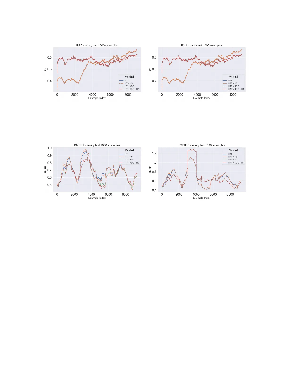
On Im balanced Regression with Ho effding T rees P antia-Marina Alc hirch Dimitrios I. Dio c hnos Univ ersity of Oklahoma {marina.alchirch,diochnos}@ou.edu Abstract Man y real-w orld applications pro vide a con tinuous stream of data that is subsequently used by machine learning mo dels to solve regression tasks of interest. Hoeffding trees and their v ariants hav e a long-standing tradition due to their effectiveness, either alone or as base mo dels in broader ensembles. A t the same time a recent line of work in batc h learn- ing has shown that kernel density estimation (KDE) is an effective approac h for smo othed predictions in im balanced regression tasks [ 43 ]. Moreo ver, another recent line of work for batc h learning, called hier ar chic al shrinkage (HS) [ 1 ], has introduced a p ost-hoc regular- ization metho d for decision trees that does not alter the structure of the learned tree. Using a telescoping argument we cast KDE to streaming environmen ts and extend the implemen tation of HS to incremen tal decision tree mo dels. Armed with these extensions w e inv estigate the p erformance of decision trees that may enjoy such options in datasets commonly used for regression in online settings. W e conclude that KDE is beneficial in the early parts of the stream, while HS hardly , if ever, offers p erformance b enefits. Our co de is publicly a v ailable at: h ttps://gith ub.com/marinaAlchirc h/DSF A_2026 . Keyw ords: Online learning, Imbalanced regression, Hoeffding trees 1 In tro duction W e liv e in a w orld where sensors monitor the environmen t and our activities and generate data that hav e the p oten tial to impro ve and transform our liv es. In this context w e find mac hine learning and data mining algorithms v ery b eneficial, as suc h algorithms can capture imp or- tan t prop erties and patterns on the data that in turn ma y giv e rise to certain phenomena of in terest. Mining such con tinuous flo ws of information gives rise to online mac hine learning algorithms and mining on data str e ams . Due to adv ances in data stream mining sev eral fields ha ve b enefited by deploying systems that use suc h mechanisms; e.g., credit score calcula- tion [ 3 ], fraud detection [ 27 ], human activit y recognition [ 25 ], clinical decision supp ort [ 16 ], energy pricing [ 39 ], and reducing the energy fo otprint of mining methods on data streams themselv es [ 18 ], just to name a few. A t the same time, w orking with imb alanc e d data is a constant nuisance for machine learn- ing and data mining applications. Imbalanced data arise when the lab els asso ciated with the observ ations that are collected, are skew ed fav oring certain categories or certain ranges of v alues. Researc h on im balanced data has focused primarily on classification problems; e.g., anomaly detection [ 26 ], e-commerce [ 5 ], infan ts’ surviv al [ 19 ], and man y others. Ho wev er, in vestigating im balanced data makes a lot of sense in regression tasks as well. F or example, 1 one ma y wan t to predict the age of an individual by ha ving access to their facial image [ 35 ], or predict w eather phenomena suc h as hail size or wind in tensit y [ 30 ]. Our work fo cuses at the intersection of the ab o ve tw o fields. W e inv estigate p opular meth- o ds that generate decision trees incremen tally and hav e b een developed with ideas for mining data streams and combine suc h mec hanisms with recen t adv ances developed for batc h learn- ing: (i) regularization of decision trees using hierarc hical shrink age [ 1 ], and (ii) approximating sk ewed distributions using kernel density estimation (KDE) [ 43 ]. Belo w w e summarize our con tributions. Con tributions. First, we implemen t hierarc hical shrink age on incremen tal decision trees that are a v ailable in the scikit m ultiflow library [ 32 ]. Second, w e revisit KDE and make it applicable to mining algorithms that op erate on streaming data. Third, by combining the abov e techniques we achiev e improv ed p erformance of incremental decision tree algorithms on im balanced regression tasks for streaming data. While we ac hiev e improv ed p erformance in suc h tasks, our main finding is that KDE helps with the improv ed predictions a lot, whereas hierarchical shrink age hardly - if ever - helps. Finally , our co de is publicly a v ailable for any one to w ork with: https://gith ub.com/marinaAlc hirch/DSF A_2026 . 2 Related W ork Incremen tal decision trees ha ve a long line of research going bac k to at least the 80’s [ 37 , 41 ]. Ho wev er, perhaps the most important incremental decision tree learning algorithm is that of Ho effding trees [ 15 ] and their v arian ts. Ho effding trees pro cess data that arriv e in a stream and b y using Ho effding’s inequalit y a decision is b eing made as to when the difference in information gain (or some other relev an t criterion) b et ween the b est-split attribute and the second-b est split attribute is sufficiently high to justify such a split. Sev eral extensions of the Ho effding trees ha ve been dev elop ed, primarily to deal with concept drift [ 7 , 17 , 21 , 22 ], but atten tion has also b een paid for parallelization [ 4 ], reduced complexity [ 2 ], or improv ed classification accuracy [ 29 ]. In parallel, a tremendous wealth of metho ds has b een dev elop ed for mining knowledge from imbalanced data. Perhaps the most well-kno wn metho d for dealing with class imbalance is Syn thetic Minorit y Oversampling T echnique (SMOTE) in whic h synthetic data are b eing created so that ov ersampling of the minority class can happ en [ 11 ]. SMOTE also has a v arian t for regression [ 40 ]. Ho w ever, many more metho ds ha ve been dev elop ed, including informed under-sampling the ma jorit y class [ 28 ], sampling based on clusters [ 23 ], re-weigh ting [ 42 ], mo difying the margin of the separation b oundary [ 9 ], or more theoretical approaches [ 10 , 12 – 14 ]. In addition, a recen t line of work is using kernel density estimation (KDE) for smo othing the predicted labels on learned mo dels [ 35 , 43 ], but has b een applied only in batc h settings where all the information is a v ailable ahead of time. W e draw inspiration from this last approac h so that we can smo oth the predicted lab els b y forming sk etches of the distribution using small sequences of examples tak en from the stream. Finally , a useful w ay for regularizing decision trees is that of pruning [ 8 , 31 , 36 ]. How ev er, pruning has not b ecome p opular for incremen tal decision trees, b y virtue of the fact that one needs to train a complete tree and then try to work backw ards b y pruning appropri- ate branches that ma y in fact increase the generalization abilit y of the tree. Nev ertheless, a 2 promising metho d that was recen tly developed for regularizing decision trees is that of hier- ar chic al shrinkage (HS) [ 1 ] where ev ery no de from the ro ot to the leaf of the decision tree has some amoun t of say in the final prediction. This new approac h is a p ost-ho c regularization tec hnique that do es not require the construction of a full tree, or p erforming costly op erations suc h as pruning certain branches or generated rules, and one can apply it to incremental decision trees provided some necessary statistics from the stream are b eing recorded. F or this reason, as far as we know, for the first time w e integrate this method to incremental decision trees and in vestigate its effect on predictiv e accuracy . This is coupled with the inclusion of KDE as an additional metho d for smo othing the predicted labels in im balanced domains. 3 Preliminaries W e use multisets for collections of ob jects that ma y contain multiple copies of the same ob ject. Con trary to regular sets, multisets allow elements to app ear with multiplic ities b ey ond 1. F or example, S = {{ x 1 , x 1 , x 2 }} is a multiset where we can find tw o copies of the instance x 1 and one copy of the instance x 2 . Similar to sets, the order in whic h the elemen ts are listed does not matter; e.g., S = {{ x 1 , x 1 , x 3 }} = {{ x 1 , x 3 , x 1 }} . F or a more compact represen tation, w e ma y also denote the multiplicit y of each element in a multiset using a pair of brack ets; e.g., S = {{ x 1 , x 3 , x 1 }} = {{ ( x 1 , 2) , ( x 3 , 1) }} . The c ar dinality | S | of a multiset S is the total n umber of elements in S taking in to account their m ultiplicities; e.g., if S = {{ ( x 1 , 2) , ( x 3 , 1) }} , then | S | = 2 + 1 = 3 . Using m ultisets w e hav e the ability to appro ximate pr ob ability density functions (p dfs) that gov ern certain domains by keeping trac k of empiric al densities broader domains. In these cases w e will adopt the m ultiset notation and explicitly indicate that certain elements do not app ear at all, using 0 for their multiplicities. F or example, in an instance space X = { x 1 , x 2 , x 3 , x 4 } using the collection of instances S = {{ ( x 1 , 2) , ( x 3 , 1) }} , we hav e the empirical densit y ˜ f S ( X ) = { ( x 1 , 2) , ( x 2 , 0) , ( x 3 , 1) , ( x 4 , 0) } . With m Z ( z ) w e denote the multiplicit y of z in Z ; e.g., m ˜ f S ( X ) ( x 1 ) = 2 in the previous example. Kernel Densit y Estimation (KDE). Kernels provide an easy w ay for similarity com- parisons b et ween instances. By storing instances in certain windows w e can pro vide smo oth estimates on imbalanced distributions for lab el v alues; including v alues that w e may hav e not seen. In general, the kernel density estimation (KDE) [ 34 ] using some arbitrary k ernel K , p oin ts z i ∈ S from some m ultiset S , and a query point q , is accomplished via the following: ˆ f S,K,h ( q ) = 1 | S | X ( z i ,m i ) ∈ S m i · K h ( q − z i ) = 1 | S | h X ( z i ,m i ) ∈ S m i · K  q − z i h  , (1) where h is the b andwidth and its role is to provide some scaling on the use of the k ernel that is used in ( 1 ). Small v alues of h mak e the estimate sensitive to individual data points, whereas large v alues of h provide a smo other estimate, by spreading the influence of eac h data p oint o ver a wider region of the dataset. W e work with the Gaussian and the Epanechnik ov kernel. The appro ximation on the labels as explained abov e is called LDS in [ 43 ]. F urthermore, w e ma y b e using binning so that w e can map individual lab el v alues to p oten tially broader in terv als in whic h these v alues fall. This is a standard tec hnique, e.g., [ 43 ]. 3 Algorithm 1 Incremental KDE Require: Windo w W = { ( x 1 , y 1 ) , ( x 2 , y 2 ) , . . . , ( x m , y m ) } , bandwidth h , k ernel K , and a structure of B groups of bins. Ensure: Smo othed weigh ts ˆ f n,K,h ( b ) for each bin b ∈ B , where n is num ber of examples that w e hav e seen in the stream so far. 1: for target q i ∈ W do 2: Put target q i in to a bin b 3: Compute ˆ f n + i,K,h ( b ) as sho wn in ( 2 ) 4: return { ˆ f n + m,K,h ( b ) } , for all b ∈ B Letting m and M b e the minim um and maximum v alues of the lab els in the dataset, r b e the range of bins, and i ⋆ = ⌊ ( M − m ) /r ⌋ , we ha ve that the different bins corresp ond to the in terv als b i = [ m + ir, m + ( i + 1) r ) for i ∈ { 0 , 1 , . . . , i ⋆ } and b i ⋆ +1 = [ m + ( i ⋆ + 1) r, m + ( i ⋆ + 2) r ] = [ m + ( i ⋆ + 1) r , M ] . Finally , as ( 1 ) is ultimately calculating an av erage, one can telescop e the sum and focus on the influence of the last quan tit y considered. This is particularly useful for streams as we hav e access to new information. In this case, ( 1 ) is conv erted to the follo wing form ula, where by changing slightly the notation and using n in the first subscript we denote the fact that we ha v e seen n examples so far from the stream: ˆ f n,K,h ( q ) = ˆ f n − 1 ,h ( q ) + 1 n  1 h K  q − z n h  − ˆ f n − 1 ,h ( q )  . (2) Th us, we are able to implemen t KDE incremen tally; Algorithm 1 has the details. Ho effding T rees and V arian ts. The most w ell-kno wn incremental decision tree learning algorithm is that of Ho effding trees (HT s) [ 15 ] and their v arian ts. This class of algorithms uses Hoeffding’s b ound as an indicator for when to split a no de. Letting R b e the range of the optimization function that is used for determining the splits in the tree that is being constructed (e.g., R = 1 in the case of information gain for binary classification) then one lo oks at the difference in that optimization function b etw een the best and second b est attribute that are candidates for the split and if that v alue is larger than ϵ = q R 2 ln(1 /δ ) 2 n , then one can ha ve confidence at least 1 − δ that the split on the b est-attribute is indeed the most b eneficial and therefore pro ceeds on adopting that split in the tree from that p oint on wards. A v ariant of the original Hoeffding tree algorithm that we also consider in this pap er is the Ho effding A daptive T r e e (HA T) [ 7 ]. HA T is using an ADWIN [ 6 ] window in order to b e able to track concept drift. In general, HA T is considered sup erior to CVFDT [ 21 ], which is another v arian t of HT that handles drift, and perhaps for this reason it CVFDT is not implemented y et in scikit-m ultiflow [ 32 ], which we use for our w ork. Regularization of Decision T rees Using Hierarchical Shrink age. As mentioned ear- lier, hierarchical shrink age (HS) [ 1 ] is a recen t regularization tec hnique that do es not alter the structure of the learned tree. Letting N ( t ) b e the n umber of samples in some no de t of a decision tree D T and E t [ y ] to b e the mean resp onse in no de t , then, the prediction of the tree on an instance x is D T ( x ) = E t 0 [ y ] + P L l =1  E t l [ y ] − E t l − 1 [ y ]  . HS mo difies this prediction 4 to D T λ ( x ) = E t 0 [ y ] + L X l =1 E t l [ y ] − E t l − 1 [ y ] 1 + λ/ N ( t l − 1 ) , (3) for some h yp er-parameter λ that p erforms the regularization. Thus, the no des in the path from root to leaf to ha v e an amoun t of sa y in the final prediction. 4 The Online Learning Pro cess That W e Study Our idea for tuning relies on the simple idea of F ol low-the-L e ader (FTL) algorithm [ 38 ]. The idea of FTL is that sev eral mo dels are b eing ran in parallel and the prediction that w e are making at an y p oin t in time aligns with the model that app ears to be b eha ving b est at that p oin t in time (e.g., because it has the low est cum ulativ e loss so far). Coming back to tuning the hyper-parameters of a mo del using examples from a stream, w e are p erio dically using some p ortions of the stream to tune our learned mo del and at the end of each suc h tuning phase w e use the hyper-parameter v alues that p erformed b est during the last tuning phase. This idea is describ ed in Algorithm 2 . Hence, the learning pro cess on the stream of examples that we ha ve access to is guided by a parameter that indicates for how long tuning should happ en as w e receiv e examples from the stream, as well as ho w frequen tly suc h an operation should happ en. This latter property is another parameter which corresp onds to the num b er of examples that we will w ork with from the stream in a predict-then-train fashion alone, without performing any tuning during that perio d. These t wo parameters are called s t and s ′ t resp ectiv ely in Algorithm 2 . The mo del that w e learn and w e use for predictions is denoted b y M in the pseudoco de. Ho wev er, M is the result of the selection of the b est p erforming mo del among a p o ol of mo dels T . Hence, in Line 3 w e initialize T with all p ossible instantiations of our base learning mo del (e.g., Ho effding tree) and all p ossible combi nations of v alues for the different hyper-parameters that will b e used to select the b est among them. In other w ords, during the tuning phase of the algorithm w e p erform “grid searc h” so that every point in the grid corresponds to the same base mo del but with different v alues on the hyper-parameters that we use. The catch is that instead of actually p erforming “grid search” sequentially we are p erforming this search in parallel b ecause we are running all the mo dels in T in parallel. Therefore, one such grid p oin t ma y , e.g., corresp ond to a Ho effding tree base mo del, coupled with KDE that uses a Gaussian k ernel that has bandwidth h and moreov er we are using bins of range r and no hierarchical shrink age ( λ = 0 ). Algorithm 2 has all these details in pseudo-code. 5 Exp erimen ts Datasets. W e p erform exp erimen ts using the datasets of California Housing [ 24 ], Electric P ow er Consumption (E-Po w er) [ 20 ], and the New Y ork T axi (NY T axi) [ 33 ]. The California Housing dataset has 20 , 640 instances and 8 features. Ho wev er, w e drop 5 instances from this sequence b ecause they appeared to be grossly misleading outliers and this w ay we obtain a stream of 20 , 635 examples. The electric pow er consumption dataset has in total 2 , 0752 , 59 instances and 9 features, but for our exp erimen ts w e use the stream of the first 100 , 000 examples from this dataset. Regarding the NY taxi dataset, its size gets updated annually . 5 Algorithm 2 Online-Learning Pro cess & F ollow-the-Leader T uning Require: Stream S = { ( x 1 , y 1 ) , ( x 2 , y 2 ) , . . . , ( x n , y n ) , . . . } of labeled examples, a set P of parameters, a tuning window size s t , and no-tuning window size s ′ t . 1: Initialize a model M 2: M.parameters ← [] 3: Initialize all differen t models T based on P 4: i ← 1 5: tune _ star t _ idx ← 1 6: tune _ end _ idx ← s t 7: for ev ery example ( x i , y i ) in stream S do 8: if i ≥ tune _ star t _ idx and i ≤ tune _ end _ idx then 9: j ← 1 10: lo west_error ← ∞ 11: b est_model ← empt y_mo del 12: while j ≤ s t do 13: Predict-then-train with ev ery model t ∈ T 14: if low est_error ≥ t.error then 15: lo w est_error ← t.error 16: best_mo del ← t 17: j ← j + 1 18: i ← i + s t 19: tune _ star t _ idx ← tuning _ star t _ idx + s t + s ′ t 20: tune _ end _ idx ← tuning _ star t _ idx + s t − 1 21: M.setP arameters(b est_mo del.parameters) 22: else 23: Predict-then-T rain on example ( x i , y i ) with M 24: i ← i + 1 A t the time of the writing it had 1 , 458 , 644 examples and w e ha ve used the first 20 , 000 examples as a stream for our exp eriments. F or sho wcasing the imbalance in these datasets w e plot the frequencies of the target v alues that are contained inside bins using range of bin r = 0 . 2 . W e presen t these plots in Figure 1 . Learning Metho ds T ested. W e use HT and HA T as base models in Algorithm 2 and w e equip b oth of these mo dels with KDE for smoothing the imbalanced lab el distribution of the stream as well as HS for regularizing the predictions. In our exp erimen ts we also equip these t wo base models with KDE alone or HS alone as a w ay of p erforming an ablation study for our results. Regarding incremental KDE w e use a tum bling windo w whose size we treat as a h yp er-parameter. On the T uning Windo w and Hyp er-Parameter T uning. In our exp erimen ts w e ha v e opted for four p erio ds of tuning the hyper-parameters of our mo dels. F or a dataset S that we treat as a stream, we use tuning windo w size equal to min ( ⌊ | S | / 8 ⌋ , 3000) . 6 (a) California Housing (b) E-Po w er (c) NY T axi Figure 1: F requency of targets con tained in bins of range r = 0 . 2 for all datasets. This window size translates to 2 , 579 examples in the California housing dataset, 3 , 000 examples in the electric p o wer dataset, and 2 , 500 examples in the NY taxi dataset. In each tuning window we use the following v alues to choose from for the hyperparameters that w e use: (i) for range of bin r ∈ { 0 , 0 . 1 , 0 . 2 , 0 . 5 , 1 } , where 0 in this con text means that we don’t p erform binning in our targets, but every target is simply its o wn bin, (ii) λ ∈ { 0 , 0 . 1 , 1 , 10 , 15 , 25 } , where 0 is for not predicting with HS and predict with initial mo del, (iii) h ∈ { 10 , 50 , 100 } , and (iv) for (tumbling) windo w size | W | ∈ { 50 , 100 , 200 } . F or simple KDE w e do not tune on λ and for simple HS we only tune on λ . Exp erimen tal Results and Discussion. T able 1 presents our o v erall results for the ex- p erimen ts that we ran. As sho wn in the table, KDE is con tributing a lot in the decrease of the error (and increase of R 2 score), but hierarc hical shrink age pro vides v ery small benefit and only the case of the NY taxi dataset. F o cusing on the NY taxi dataset we pro vide the follo wing plots. Figure 2 presen ts the ro ot mean squared error (RMSE) of the learned mo del (as describ ed in Algorithm 2 , when HT or HA T are used as base mo dels). Figure 3 presents the RMSE as it is calculated o ver the last 1,000 examples in the stream. This allows us to observ e the error in the region that app ears to be flat in Figure 2 . Finally , Figure 4 presents R 2 as this is calculated again ov er the last 1,000 examples in the stream. 7 Mo del MAE RMSE R 2 HT 0.4681 0.6739 0.6556 HA T 0.4495 0.6735 0.6559 HT + HS 0.4926 0.7278 0.5982 HA T + HS 0.4741 0.6962 0.6323 HT + KDE 0.4342 0.6497 0.6798 HA T + KDE 0.3923 0.6806 0.6487 HT + KDE + HS 0.4362 0.6522 0.6773 HA T + KDE + HS 0.3974 0.6837 0.6455 (a) California Housing Mo del MAE RMSE R 2 HT 0.0825 0.2200 0.9729 HA T 0.2251 0.3840 0.9175 HT + HS 0.1024 0.2334 0.9695 HA T + HS 0.2450 0.4015 0.9098 HT + KDE 0.0725 0.1639 0.9849 HA T + KDE 0.0939 0.2182 0.9733 HT + KDE + HS 0.0727 0.1643 0.9848 HA T + KDE + HS 0.0940 0.2184 0.9733 (b) E-Po w er Mo del MAE RMSE R 2 HT 0.3918 0.5189 0.5197 HA T 0.3918 0.5189 0.5197 HT + HS 0.3918 0.5189 0.5197 HA T + HS 0.3918 0.5189 0.5197 HT + KDE 0.3726 0.4930 0.5665 HA T + KDE 0.3726 0.4930 0.5665 HT + KDE + HS 0.3724 0.4925 0.5673 HA T + KDE + HS 0.3724 0.4925 0.5673 (c) NY T axi T able 1: Metrics of mo dels in the differen t datasets tested. Gr e en colored v alues indicate the b est p erformance from a model across a column, and b old styled v alues the second best. In the other t wo datasets (California Housing and E-P o wer) w e observe a similar drastic decrease in the RMSE in the b eginning of the plot and therefore one obtains results similar to Figure 2 and for this reason w e do not include these plots. Ho wev er, w e do include the RMSE as it is calculated ov er the last 1,000 examples in the stream so that w e can observ e the p erformance of the prop osed method this wa y . These plots app ear in Figures 5 and 6 . As w e can see in the pictures, KDE helps with the learning pro cess a lot in the b eginning so that w e hav e b etter predictions on im balanced data earlier in the stream. Moreov er, o verall, w e observe that KDE, p oten tially with the inclusion of HS, helps a lot the base HT and HA T algorithms that w e hav e tested across all the datasets that we ha v e tested. W e do not plot R 2 due to space considerations. 6 Conclusions and F uture W ork W e recast recen t adv ances in b atch le arning regarding im balanced data and regularization of decision trees, in str e aming sc enarios . W e are prop osing the inclusion of KDE and p oten tially HS in incremental decision tree learning algorithms. W e hav e seen that KDE improv es signif- ican tly the p erformance of all mo dels used in all three dataset cases. How ev er, HS pro vides minimal gains, if at all. W e anticipate that the observed b enefits will translate to similar b enefits in random forests or other ensem bles of such tree-based mo dels. W e note that KDE do es not naturally extend to pure classification problems and it is a question if one can find a new method that can further improv e the p erformance of suc h incremental mo dels with, or without, the inclusion of HS. 8 (a) RMSE of all HT based mo dels. (b) RMSE of all HA T based models. Figure 2: Comparison of RMSE plots b et w een HT and HA T based mo dels for the NY T axi dataset. (a) RMSE after every 1000 examples of all HT based mo dels. (b) RMSE after ev ery 1000 examples of all HA T based mo dels. Figure 3: Comparison of RMSE after every 1000 examples plots b et ween HT and HA T based mo dels for the NY T axi dataset. A ckno wledgemen ts. This material is based up on work supported b y the U.S. National Science F oundation under Grant No. RISE-2019758. This w ork is part of the NSF AI Insti- tute for Research on T rust w orthy AI in W eather, Climate, and Coastal Oceanography (NSF AI2ES). Disclosure of In terests. The authors hav e no comp eting in terests to declare that are relev an t to the conten t of this article. References [1] Abhineet Agarwal, Y an Sh uo T an, Omer Ronen, Chandan Singh, and Bin Y u. Hierar- c hical Shrink age: Improving the accuracy and interpretabilit y of tree-based mo dels. In ICML , volume 162 of Pr o c e e dings of Machine L e arning R ese ar ch , pages 111–135. PMLR, 2022. 9 (a) R 2 score after every 1000 examples of all HT based mo dels. (b) R 2 score after every 1000 examples of all HA T based mo dels. Figure 4: Comparison of R 2 score after ev ery 1000 examples plots b et ween HT and HA T based models for the NY T axi dataset. (a) RMSE after every 1000 examples of all HT based mo dels. (b) RMSE after ev ery 1000 examples of all HA T based mo dels. Figure 5: Comparison of RMSE after every 1000 examples plots b et ween HT and HA T based mo dels for the California Housing dataset. [2] Jean Paul Barddal and F abrício Enembrec k. Learning regularized ho effding trees from data streams. In SAC , pages 574–581. A CM, 2019. [3] Jean P aul Barddal, Lucas Lo ezer, F abrício Enem breck, and Riccardo Lanzuolo. Lessons learned from data stream classification applied to credit scoring. Exp ert Syst. Appl. , 162: 113899, 2020. [4] Y ael Ben-Haim and Elad T om-T ov. A Streaming P arallel Decision T ree Algorithm. J. Mach. L e arn. R es. , 11:849–872, 2010. [5] Liliy a Besalev a and Alfred C. W eav er. Classification of im balanced data in E-commerce. In 2017 Intel liSys , pages 744–750. IEEE, 2017. [6] Alb ert Bifet. A daptive learning and mining for data streams and frequent patterns. SIGKDD Explor. Newsl. , 11(1):55–56, Nov ember 2009. ISSN 1931-0145. 10 (a) RMSE after every 1000 examples of all HT based mo dels. (b) RMSE after ev ery 1000 examples of all HA T based mo dels. Figure 6: Comparison of RMSE after every 1000 examples plots b et ween HT and HA T based mo dels for the E-P ow er dataset. [7] Alb ert Bifet and Ricard Gav aldà. Adaptiv e Learning from Ev olving Data Streams. In ID A , volume 5772 of LNCS , pages 249–260. Springer, 2009. [8] Leo Breiman, J. H. F riedman, R. A. Olshen, and C. J. Stone. Classific ation and R e gr es- sion T r e es . W adsw orth, 1984. ISBN 0-534-98053-8. [9] Kaidi Cao, Colin W ei, Adrien Gaidon, Nikos Aréchiga, and T engyu Ma. Learning Im bal- anced Datasets with Lab el-Distribution-A w are Margin Loss. In NeurIPS , pages 1565– 1576, 2019. [10] Kamalik a Chaudhuri, Kartik Ah uja, Martín Arjo vsky , and Da vid Lopez-Paz. Why does Thro wing A w ay Data Improv e W orst-Group Error? In ICML , volume 202 of Pr o c e e dings of Machine L e arning R ese ar ch , pages 4144–4188. PMLR, 2023. [11] Nitesh V. Chawla, Kevin W. Bowy er, La wrence O. Hall, and W. Philip Kegelmeyer. SMOTE: Synthetic Minority Over-sampling T ec hnique. J. A rtif. Intel l. R es. , 16:321– 357, 2002. [12] Lee Cohen, Yisha y Mansour, Sha y Moran, and Han Shao. Probably Approximately Precision and Recall Learning. CoRR , abs/2411.13029, 2024. [13] Corinna Cortes, Anqi Mao, Mehry ar Mohri, and Y utao Zhong. Balancing the Scales: A Theoretical and Algorithmic F ramew ork for Learning from Im balanced Data. In ICML , v olume 267 of Pr o c e e dings of Machine L e arning R ese ar ch . PMLR / Op enReview.net, 2025. [14] Dimitrios I. Dio c hnos and Theo dore B. T rafalis. Learning Reliable Rules under Class Im balance. In SDM , pages 28–36. SIAM, 2021. [15] P edro M. Domingos and Geoff Hulten. Mining high-speed data streams. In Raghu Ramakrishnan, Salv atore J. Stolfo, Rob erto J. Bay ardo, and Ismail Parsa, editors, KDD , pages 71–80. A CM, 2000. 11 [16] Simon F ong, Y ang Zhang, Jinan Fiaidhi, Osama Mohammed, and Sabah Mohammed. Ev aluation of stream mining classifiers for real-time clinical decision support system: a case study of blo o d glucose prediction in diab etes therapy . BioMe d R ese ar ch Interna- tional , 1:274193, 2013. [17] João Gama, Ricardo F ernandes, and Ricardo Rocha. Decision trees for mining data streams. Intel l. Data A nal. , 10(1):23–45, 2006. [18] Ev a García-Martín, Alb ert Bifet, and Niklas La vesson. Energy mo deling of Ho effding tree ensem bles. Intel l. Data Anal. , 25(1):81–104, 2021. [19] P ascale Gourdeau, Lara J. Kanbar, Wissam Shalish, Guilherme M. Sant’Anna, Rob ert E. Kearney , and Doina Precup. F eature selection and o v ersampling in analysis of clinical data for extubation readiness in extreme preterm infants. In EMBC , pages 4427–4430, 2015. [20] Georges Hebrail and Alice Berard. Individual Household Electric P ow er Consumption. UCI Mac hine Learning Repository , 2006. [21] Geoff Hulten, Laurie Sp encer, and P edro M. Domingos. Mining Time-Changing Data Streams. In KDD , pages 97–106. A CM, 2001. [22] Elena Ikonomo vsk a, João Gama, and Saso Dzeroski. Learning mo del trees from evolving data streams. Data Min. Know l. Disc ov. , 23(1):128–168, 2011. [23] T aeho Jo and Nathalie Japko wicz. Class im balances versus small disjuncts. SIGKDD Explor ations , 6(1):40–49, 2004. [24] R. Kelley Pace and Ronald Barry . Sparse spatial autoregressions. Statistics & Pr ob ability L etters , 33(3):291–297, 1997. ISSN 0167-7152. [25] Martin Khannouz and T ristan Glatard. A Benchmark of Data Stream Classification for Human A ctivity Recognition on Connected Ob jects. Sensors , 20(22):6486, 2020. [26] W ael Khreich, Eric Granger, Ali Miri, and Rob ert Sab ourin. Iterative Bo olean com bina- tion of classifiers in the R OC space: An application to anomaly detection with HMMs. Pattern R e c o gnition , 43(8):2732–2752, 2010. [27] Naeimeh Laleh and Mohammad Ab dollahi Azgomi. A T axonomy of F rauds and F raud Detection T ec hniques. In ICISTM , volume 31 of CCIS , pages 256–267. Springer, 2009. [28] Xu-Ying Liu, Jianxin W u, and Zhi-Hua Zhou. Exploratory Undersampling for Class- Im balance Learning. IEEE T r ans. Syst. Man Cyb ern. Part B , 39(2):539–550, 2009. [29] Chaitan ya Manapragada, Geoffrey I. W ebb, and Mahsa Salehi. Extremely F ast Decision T ree. In KDD , pages 1953–1962. A CM, 2018. [30] Am y McGov ern, Kimberly L. Elmore, Da vid John Gagne, Sue Ellen Haupt, Christo- pher D. Karstens, Ryan Lagerquist, T ravis Smith, and John K. Williams. Using artificial in telligence to impro ve real-time decision-making for high-impact weather. Bul letin of the Americ an Mete or olo gic al So ciety , 98(10):2073 – 2090, 01 Oct. 2017. 12 [31] T om M. Mitchell. Machine le arning . Series in Computer Science. McGraw-Hill, 1997. ISBN 978-0-07-042807-2. [32] Jacob Montiel, Jesse Read, Alb ert Bifet, and T alel Ab dessalem. Scikit-m ultiflo w: A m ulti-output streaming framew ork. JMLR , 19(72):1–5, 2018. [33] New Y ork City T axi and Limousine Commission. Tlc trip record data. https://www. nyc.gov/site/tlc/about/tlc- trip- record- data.page , 2009-2025. [34] Eman uel Parzen. On estimation of a probability density function and mo de. The Annals of Mathematic al Statistics , 33(3):pp. 1065–1076, 1962. ISSN 00034851. [35] Ruizhi Pu, Gezheng Xu, Ruiyi F ang, Bingkun Bao, Charles Ling, and Boyu W ang. Lev eraging Group Classification with Descending Soft Lab eling for Deep Im balanced Regression. In AAAI , pages 19978–19985. AAAI Press, 2025. [36] J. Ross Quinlan. C4.5: Pr o gr ams for Machine L e arning . Morgan Kaufmann, 1993. ISBN 1-55860-238-0. [37] Jeffrey C. Schlimmer and Douglas H. Fisher. A Case Study of Incremen tal Concept Induction. In AAAI , pages 496–501. Morgan Kaufmann, 1986. [38] Shai Shalev-Sh wartz. Online learning and online conv ex optimization. F ound. T r ends Mach. L e arn. , 4(2):107–194, F ebruary 2012. ISSN 1935-8237. [39] Yibin Sun, Heitor Murilo Gomes, Bernhard Pfahringer, and Alb ert Bifet. Real-Time Energy Pricing in New Zealand: An Evolving Stream Analysis. In PRICAI , v olume 15285 of LNCS , pages 91–97. Springer, 2024. [40] Luís T orgo, Rita P Ribeiro, Bernhard Pfahringer, and Paula Branco. Smote for regres- sion. In Portuguese c onfer enc e on artificial intel ligenc e , pages 378–389. Springer, 2013. [41] P aul E. Utgoff. ID5: An Incremental ID3. In ICML , pages 107–120, 1988. [42] Y u-Xiong W ang, Dev a Ramanan, and Martial Heb ert. Learning to Mo del the T ail. In NeurIPS , pages 7029–7039, 2017. [43] Y uzhe Y ang, Kaiwen Zh a, Ying-Cong Chen, Hao W ang, and Dina Katabi. Delving in to Deep Im balanced Regression. In ICML , v olume 139 of PMLR , pages 11842–11851. PMLR, 2021. 13