EEG-SeeGraph: Interpreting functional connectivity disruptions in dementias via sparse-explanatory dynamic EEG-graph learning

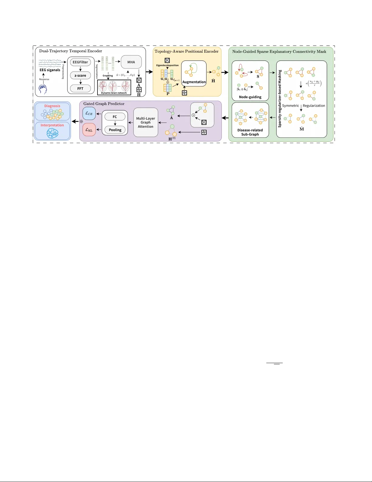
EEG-SEEGRAPH: INTERPRETING FUNCTIONAL CONNECTIVITY DISR UPTIONS IN DEMENTIAS VIA SP ARSE-EXPLANA TOR Y D YNAMIC EEG-GRAPH LEARNING F engcheng W u 1 , Zhenxi Song 1 ∗ , Guoyang Xu 1 , Kaisong Hu 1 , Zirui W ang 1 , Y i Guo 2 and Zhiguo Zhang 1 1 Harbin Institute of T echnology , Shenzhen, China 2 Institute of Neurological Diseases, Shenzhen Bay Laboratory , Shenzhen, China ABSTRA CT Robust and interpretable dementia diagnosis from noisy , non- stationary electroencephalography (EEG) is clinically essential yet remains challenging. T o this end, we propose SeeGraph , a S parse- E xplanatory dynamic E EG- graph network that models time-ev olving functional connecti vity and emplo ys a node-guided sparse edge mask to rev eal the connections that dri ve the diagnostic decision, while remaining rob ust to noise and cross-site variability . SeeGraph comprises four components: 1) a dual-trajectory tempo- ral encoder that models dynamic EEG with two streams, with node signals capturing regional oscillations and edge signals capturing interregional coupling; 2) a topology-aware positional encoder that deriv es graph-spectral Laplacian coordinates from the fused connec- tivity and augments the node embeddings; 3) a node-guided sparse explanatory edge mask that gates the connecti vity into a compact subgraph; and 4) a gated graph predictor that operates on the spar- sified graph. The framework is trained with cross-entropy together with a sparsity regularizer on the mask, yielding noise-robust and interpretable diagnoses. The ef fectiv eness of SeeGraph is validated on public and in-house EEG cohorts, including patients with neu- rodegenerati ve dementias and healthy controls, under both raw and noise-perturbed conditions. Its sparse, node-guided explanations highlight disease-rele v ant connections and align with established clinical findings on functional connectivity alterations, thereby of- fering transparent cues for neurological ev aluation. Index T erms — EEG, Graph neural networks, Explainable AI, Dynamic functional connectivity , Dementia 1. INTRODUCTION Electroencephalography (EEG) offers practical utility for screening and monitoring in neurode generati ve dementias such as Alzheimer’ s disease (AD) and frontotemporal dementia (FTD) [1] because it is low-cos t, non-in vasi ve, and offers high temporal resolution [2]. Identifying dementia related EEG patterns requires models that can operate on high-dimensional, noisy , and non-stationary signals. It is also valuable that such models generalize across sites[3] and yield insights that help interpret brain functional disruptions[4]. Earlier machine learning approaches relied on handcrafted spec- tral features or shallo w classifiers, which are limited in capturing complex spatio-temporal dependencies[5]. Subsequent deep learn- ing models, such as con volutional and recurrent networks, im- prov ed representation capacity yet still treated channels as grids ∗ Corresponding author: Zhenxi Song (songzhenxi@hit.edu.cn). This work was supported by the National Natural Science Foundation of China (Grant No. 62306089) and the Shenzhen Science and T echnology Program (Grant Nos. RCBS20231211090800003 and ZDSYS20230626091203008). or sequences and thus lacked explicit modeling of brain network topology . More recent graph-based methods be gan to encode inter- regional relationships, b ut many adopt static or simplified formula- tions that underutilize temporal e volution[6][7]. Since pathological information is frequently embedded in the temporal e volution of network patterns rather than fixed states, existing methods struggle to capture dynamic cross-regional interactions, which undermines generalization and robustness[8, 9, 10]. At the same time, many models operate as black boxes, making their decision processes dif ficult to trace [11, 12]. The y of fer limited insight into the dynamics of functional connecti vity and therefore fall short of clinical requirements for transparenc y and trustworthi- ness [13]. Post hoc explanation methods are often unstable or fail to faithfully reflect the model’ s reasoning [14, 15]. These limita- tions highlight the need for inherently interpretable spatio-temporal graph models that provide reliable, clinically meaningful explana- tions while maintaining strong predicti ve performance. Rob ustness to site v ariability and acquisition noise also remains insufficient, leaving a gap for approaches that are both reliable and clinically interpretable[16]. Motiv ated by dementia pathophysiology that inv olves disrupted coordinated oscillations and interregional coupling[17], we propose a sparse-explanatory dynamic EEG-graph network, SeeGraph , that jointly covers two complementary feature domains: node-lev el re- gional oscillatory acti vity and edge-lev el amplitude-based interre- gional coupling. The model forms time-varying brain graphs, learns compact explanatory subnetworks while performing diagnosis, and is designed to improv e interpretability and stability under noise and cross-site variability . The main contributions of this w ork are: • W e introduce SeeGraph , an intrinsically explainable dynamic EEG-graph network that models time-v arying brain networks for dementia diagnosis while localizing connectivity disruptions. • Quantitatively , across a public cohort and an in-house clinical co- hort, SeeGraph achieves state-of-the-art accuracy under both raw and noise-perturbed EEG, demonstrating cross-site robustness. • Qualitatively , SeeGraph yields sparse, node-guided edge-lev el explanations that identify disease-relevant functional connectivity consistent with clinical evidence. 2. METHOD The ov erall architecture of SeeGraph , an intrinsically explainable dynamic EEG-graph network, is illustrated in Fig. 1. First, the dual- trajectory temporal encoder introduces two feature domains that together cover regional oscillatory activity and interre gional cou- pling. Node trajectories carry frequency domain spectra obtained Fig. 1 . Architecture of SeeGraph : dynamic EEG graphs are constructed, node and connecti vity trajectories are temporally encoded, Laplacian positional encodings augment node embeddings, and a node-guided sparse mask yields an explanatory subgraph for a gated graph predictor . The objectiv e combines diagnosis cross-entropy with a sparsity regularizer on the edge mask to learn compact, interpretable connectivity . by FFT , while edge trajectories carry Pearson correlation computed from amplitude time series; the two streams share parameters in the dual-trajectory temporal encoder to impro ve data ef ficiency and ro- bustness under noisy , limited clinical EEG. Second, the topology- aware positional encoder deri ves graph-spectral Laplacian coor - dinates from the fused edge connectivity and appends them to the node embeddings, injecting task-rele vant topological context into the node domain. Third, the node-guided sparse explanatory edge mask conditions sparsification on pairwise node embeddings instead of raw edge weights, which av oids circular dependence on the con- nectivity being gated, prevents mask degeneration, and yields faith- ful, compact explanatory subgraphs. Fourth, the gated graph pre- dictor runs graph attention on the sparsified connectivity and ag- gregates node representations into a graph-level embedding for di- agnosis. The training objective couples cross-entropy that pulls the learned edge mask toward a low retention Bernoulli prior , imple- menting an information bottleneck style constraint. 2.1. Dual-T rajectory T emporal Encoder As illustrated in Fig. 1, we z-score each channel and segment the N -channel EEG into T windo ws to form a dynamic graph sequence G = { G t } T t =1 . Each graph G t = ( V , E t , X t , A t ) is defined so that V index es the N EEG channels (node v i corresponds to one chan- nel), E t collects the functional couplings in window t , X t ∈ R N × d stacks node features with ro w i gi ven by x i,t ∈ R d encoding the activity of channel i at time t , and A t ∈ R N × N is the adjacency whose entry a ij,t quantifies the functional strength between v i and v j at time t . Unlike static methods with a fixed adjacency , we con- struct A t for each time window to preserve brain network dynamics. The dual-stream temporal encoder introduces two complemen- tary feature domains that jointly capture regional oscillatory acti vity and inter-re gional coupling. Specifically , the continuous EEG sig- nal is segmented into short, ov erlapping time windows. For each window t , we e xtract two types of features: • Node T rajectory: or each channel i and time windo w t , we ap- ply the Fast Fourier T ransform (FFT) to the windo wed signal to obtain a spectral vector x i,t ∈ R d . Stacking these vectors ov er time yields the node trajectory X i = [ x i, 1 ; . . . ; x i,T ] ∈ R T × d , which summarizes the oscillatory activity of channel i across win- dows. Stacking X i across channels produces the tensor X 1: T ∈ R T × N × d that collects all node tokens for the T windows. • Edge T rajectory: W ithin each window t , we compute the ab- solute Pearson correlation between the amplitude time series of each pair of channels ( i, j ) , producing a weighted, symmetric ad- jacency matrix A t ∈ R N × N with entries a ij,t and zero diago- nal. Stacking { A t } T t =1 ov er time yields the edge trajectory tensor A 1: T ∈ R T × N × N . For a specific pair ( i, j ) , the temporal trajec- tory a ij, 1: T = [ a ij, 1 , . . . , a ij,T ] ⊤ ∈ R T represents the ev olution of interregional coupling across windows. W e adopt absolute Pear- son correlation for its parameter-free formulation and robustness under short-window and noisy EEG conditions. After processing all T time windows, we construct a sequence of dynamic graphs G = { G t } T t =1 , whose topology ev olves. W e then apply multi-head self-attention (MHA)[18] along the temporal axis independently to each node trajectory and each connecti vity trajec- tory , capturing long-range temporal dependencies. Giv en an input sequence X = { x 1 , . . . , x T } , MHA computes weighted combina- tions of projected queries Q k , ke ys K k , and values V k , follo wed by an output projection W O [18]. Specifically , two feature streams share parameters within MHA s, improving data efficienc y and ro- bustness under noisy and limited clinical EEG conditions. MHA( X ) = Concat(head 1 , . . . , head H ) W O , (1) head k = softmax  Q k K ⊤ k √ d k  V k , (2) The dual-trajectory temporal encoder fuses temporal dependen- cies into compact representations. It yields node embeddings ¯ H ∈ R N × D that summarize each channel’ s acti vity o ver time and a fused connectivity matrix ¯ A ∈ R N × N that captures the evolution of func- tional coupling. W e compute ¯ H by av eraging the node time tokens, and we form ¯ A by taking the last time step of the edge stream, which emphasizes the most recent interregional interactions. W e compute ¯ H by averaging the node time tokens, and we form ¯ A by taking the final attention-aggregated token of the edge stream, which empha- sizes the most recent interregional interactions. 2.2. T opology-A ware P ositional Encoder This encoder deri ves Laplacian eigenv ector coordinates from the fused adjacency and concatenates them with the node embeddings, thereby injecting topology-relev ant positional cues into the node domain[19]. Giv en the temporally fused connectivity ¯ A ∈ R N × N , let D = diag( ¯ A1 ) be its degree matrix and define the (symmetric) normalized Laplacian. L = I − D − 1 2 ¯ AD − 1 2 . (3) T aking the eigendecomposition of L yields L = U Λ U ⊤ , where U = [ u 1 , . . . , u N ] is the eigenv ector matrix with columns u i ∈ R N , and Λ = diag ( λ 1 , . . . , λ N ) are the eigen values in ascending order . The Laplacian positional encodings P are then constructed by stacking the d pe eigen vectors from U that correspond to the smallest nonzero eigen values: P = [ u 2 , . . . , u d pe +1 ] ∈ R N × d pe . (4) W e then augment graph connectivity embeddings via concatenation: ¯ H ← [ ¯ H ∥ P ] ∈ R N × ( D + d pe ) . (5) By embedding both local activity and global structure, the model gains a more holistic understanding of brain dynamics. 2.3. Node-Guided Sparse Explanatory Connectivity Mask This module is designed to identify a sparse and informative net- work by learning a stochastic connecti vity mask[20]. It operates in an connectivity-wise manner , where the importance of each poten- tial connectivity is computed directly from the embeddings of its endpoint nodes. Specifically , for each potential connecti vity ( v i , v j ) , the Extrac- tor takes the corresponding time-aggregated node embeddings ¯ h i and ¯ h j from the previous stage. These two embeddings are con- catenated to form a feature v ector [ ¯ h i ⊕ ¯ h j ] that uniquely represents the connectivity . This vector is then passed through a shared Multi- Layer Perceptron (MLP) to produce a single logit s ij quantifying the connectivity’ s rele vance. Repeating this for all pairs yields the full connectivity-logit matrix S ∈ R N × N . From these logits, a differentiable binary-concr ete (Gumbel- Sigmoid) mask M ∈ (0 , 1) N × N is sampled: m ij = σ  s ij + g ij τ  , g ij ∼ Logistic(0 , 1) , (6) where τ > 0 is a temperature parameter that is annealed during training. T o ensure the resulting network is undirected, the mask is made symmetric and its diagonal is zeroed out: ˜ M = SymmZeroDiag( M ) = M + M ⊤ 2 − diag  diag( M )  . (7) T o encourage sparsity and prev ent the model from selecting all con- nectivity , a KL diver gence penalty aligns the mask distribution with a Bernoulli prior[21, 22] of mean r : L KL = 1 N ( N − 1) X i  = j h m ij log m ij r + ϵ + (1 − m ij ) log 1 − m ij 1 − r + ϵ i , (8) where ϵ ensures numerical stability . Sparsification is performed based on pairwise node embeddings rather than raw edge weights, which av oids circular dependence on the connecti vity being gated, prev ents mask degeneration, and yields reliable and compact ex- planatory brain network. 2.4. Gated Graph Predictor T o form the input graph structure for classification, we construct a gated adjacenc y matrix by applying the learned explanatory mask to the temporally fused connectivity: ˆ A = ˜ M ⊙ ¯ A , (9) where ¯ A ∈ R N × N is the dynamic connectivity matrix aggregated ov er time. This gating mechanism selecti vely retains the most rele- vant connections, and The resulting ˆ A is used in subsequent graph learning steps to guide the learning process in the network for diag- nosis. Let H (0) = [ ¯ H ∥ P ] ∈ R N × ( D + d pe ) be the initial node-feature matrix. A multi-layer GA T[23] runs on ˆ A , updating ro ws of H ( l ) as H ( l +1) i : = σ   X j ∈N ˆ A ( i ) ˆ a ij α ( l ) ij W ( l ) H ( l ) j :   , (10) where ˆ a ij is the ( i, j ) -entry of the explanatory adjacency ˆ A , α ( l ) ij are GA T attention coefficients, and W ( l ) are learnable weights.After graph-lev el pooling, we obtain a graph representation for classifica- tion and train the model by minimizing the objectiv e: L = L CE + λ KL L KL , (11) The training objective combines cross-entropy loss with a term that pulls the learned edge mask to ward a low retention Bernoulli prior, thereby implementing an information bottleneck-style constraint. Here, λ KL is a hyperparameter that balances the trade-off between predictiv e accuracy and the sparsity of the explanation. This mechanism distills the dynamic brain network into a sparse, clinically meaningful subgraph that makes explicit which connec- tions drive the diagnosis, thereby enhancing transparency and ro- bustness by filtering spurious relations. 3. EXPERIMENTS AND RESUL TS 3.1. Experimental Setup Datasets. W e used two EEG datasets. (i) AHEP A: a public resting- state EEG cohort collected at AHEP A Uni versity Hospital [29]. It includes 88 participants: 36 with AD, 23 with FTD, and 29 healthy controls (HC). Recordings were acquired in the eyes-closed condi- tion with a 19-channel 10–20 system at 500 Hz. W e treat this as a three-class classification task and report macro-averaged metrics across classes. (ii) SZPH: a clinical cohort from Shenzhen People’ s Hospital comprising EEG from patients with AD and HC. A total of 50 participants remained (30 AD, 20 HC) after diagnostic screening. Recordings used a 64-channel 10–20 system. Implementation details. W e implemented SeeGraph in PyT orch and ran all experiments on an NVIDIA R TX 3090 GPU. Evaluation was conducted on the in-house SZPH cohort and the public AHEP A cohort. Experiments were conducted independently per dataset. Dif- ferences in sampling rates and channel counts were handled via con- sistent band-limiting and spectral feature extraction. 3.2. Experimental Results T o ensure fair comparison in our subject-independent clinical set- ting, we focus on representativ e dynamic GNN and temporal base- lines rather than externally pretrained EEG foundation models. Baselines include: dynamic GNNs such as EvolveGCN-O [26], T able 1 . Performance comparison on the SZPH and AHEP A datasets under normal and noisy conditions Method SZPH Dataset ( China ) AHEP A Dataset ( Greece ) Raw (no added noise) Noisy Raw (no added noise) Noisy A CC A UROC F1 A CC A UROC F1 A CC A UROC F1 A CC A UROC F1 BIO T[24] 0.765 0.820 0.761 0.621 0.767 0.607 0.812 0.937 0.798 0.733 0.786 0.712 DCRNN[25] 0.760 0.819 0.779 0.661 0.740 0.737 0.738 0.819 0.719 0.651 0.734 0.657 EGCN[26] 0.734 0.726 0.718 0.645 0.643 0.660 0.648 0.769 0.614 0.602 0.736 0.522 CNN-LSTM 0.770 0.804 0.772 0.723 0.731 0.695 0.635 0.752 0.556 0.592 0.631 0.542 STGCN[27] 0.772 0.831 0.761 0.743 0.785 0.717 0.645 0.778 0.628 0.623 0.758 0.603 MA TT[28] 0.613 0.653 0.630 0.583 0.626 0.571 0.669 0.729 0.627 0.635 0.701 0.589 SeeGraph 0.874 0.951 0.875 0.848 0.926 0.849 0.841 0.953 0.834 0.827 0.937 0.822 T able 2 . Diagnostic utility of EEG frequenc y bands for dementia diagnosis across two cohorts Bands SZPH Dataset ( China ) AHEP A dataset ( Greece ) Raw (no added noise) Noisy Raw (no added noise) Noisy A CC A UROC F1 A CC A UROC F1 A CC A UROC F1 A CC A UROC F1 δ (Delta) 0.693 0.795 0.716 0.663 0.765 0.664 NAN NAN NAN N AN N AN N AN θ (Theta) 0.702 0.867 0.621 0.815 0.830 0.804 0.739 0.897 0.719 0.725 0.876 0.710 α (Alpha) 0.792 0.817 0.773 0.729 0.816 0.745 0.881 0.969 0.876 0.832 0.937 0.851 β (Beta) 0.828 0.887 0.818 0.785 0.862 0.764 0.827 0.948 0.820 0.789 0.895 0.763 γ (Gamma) 0.708 0.819 0.748 0.692 0.770 0.660 0.681 0.859 0.676 0.676 0.815 0.663 DCRNN [25], and STGCN [27], and temporal models including BIO T [24], CNN-LSTM, and MAtt [28]. All experiments use a subject-independent 80/20 train–test split at the subject lev el. As shown in T able 1, SeeGraph achiev es the best metrics on both the SZPH and AHEP A datasets, confirming the benefits of the two-stream temporal encoding and node-guided sparse edge gating. The same table reports rob ustness under additive Gaussian noise (zero mean, standard deviation 0.3) injected into the input signals. Under these noisy conditions, SeeGraph exhibits only minor perfor- mance de gradation, demonstrating robustness, ef fecti ve modeling of long-range temporal dependencies, and generalization across vary- ing data quality . T able 3 . Ablation study of SeeGraph Method SZPH AHEP A A CC A UROC F1 A CC A UROC F1 SeeGraph 0.874 0.951 0.875 0.841 0.953 0.834 w/o C-wise 0.855 0.938 0.862 0.823 0.904 0.805 w/o PE 0.837 0.905 0.841 0.824 0.918 0.829 w/o SR 0.770 0.864 0.761 0.812 0.937 0.798 w/o FFT 0.758 0.842 0.772 0.784 0.924 0.768 For scientific validation and clinical rele v ance, we conduct a band-wise analysis to quantify each EEG band’ s contribution to de- mentia diagnosis. Results (T able 2) shows that α , β , and δ carry the strongest diagnostic signal, θ is moderate, and γ is comparativ ely weak. In the AHEP A cohort, the δ -band is unavailable after their original preprocessing, yielding N A entries. These findings are con- sistent with clinical evidence of α attenuation, β suppression, and δ elev ation in dementia, thereby reinforcing the plausibility and inter- pretability of the learned features. W e conducted ablation experiments to assess the contrib ution of each module in SeeGraph . As sho wn in T able 3, removing any single component degrades performance, indicating complementary contributions to representation learning. Removing the connectiv- ity stream (w/o C-wise) lowers all metrics, underscoring the impor- tance of modeling inter -channel relationships. Discarding positional encodings (w/o PE) also reduces F1, sho wing that topological cues aid both accuracy and interpretability . T urning off the sparsity re gu- larizer on the edge mask (w/o SR, i.e., λ KL = 0 ) reduces A UR OC and produces denser , less faithful explanations. Omitting frequency- domain features (w/o FFT) yields a marked drop, confirming the utility of spectral information for brain dynamics. Collectively , these results support the indispensability of each module in SeeGraph . T o illustrate the model’ s explainability , we visualize disease- relev ant brain connectivity on the SZPH cohort, showing ho w SeeGraph captures and integrates temporal dependencies and interregional functional coupling. As sho wn in Fig. 2, disease- relev ant edges concentrate in fronto-temporal circuitry . AD exhibits temporal-lobe–centered clustering, whereas HC retains more inter- hemispheric bridges and a more symmetric bilateral fronto-temporal integration. Fig. 2 . SeeGraph localizes salient fronto-temporal subnetworks via a node-guided sparse mask. AD exhibits temporal-centered ipsilat- eral clustering (red), while HC sho ws more interhemispheric and bi- lateral integration (blue); darker colors indicate higher salience. 4. CONCLUSION This paper presents SeeGraph , a sparse-explanatory dynamic EEG- graph network addressing the dual challenges of robustness and interpretability in dementia diagnosis. By modeling time-varying brain networks, SeeGraph jointly captures regional oscillations and interregional coupling, extracts clinically meaningful subnetworks through a node-guided sparse masking mechanism. The model in- tegrates spectral and topological cues via a dual-trajectory encoder and Laplacian-based positional encoding, supporting transparent diagnostic reasoning. Experiments on a public and a clinical EEG cohort show that SeeGraph achieves superior performance under clean and noisy conditions. Ablation and interpretability analy- ses validate each component and the alignment of extracted patterns with clinical findings. SeeGraph thus offers a rob ust and explainable framew ork for EEG-based neurodegenerati ve disease analysis. 5. REFERENCES [1] L. Jia, T . Jiang, and C. Liu, “Pre valence, risk factors, and man- agement of dementia and mild cogniti ve impairment in adults aged 60 years or older in China: A cross-sectional study , ” The Lancet Public Health , vol. 5, no. 12, pp. e661–e671, 2020. [2] D. Cai, J. Chen, and Y . Y ang, “Mbrain: A multi-channel self- supervised learning framew ork for brain signals, ” in Pr oceed- ings of the 29th A CM SIGKDD Conference on Knowledge Dis- covery and Data Mining , 2023, pp. 130–141. [3] M. Hata, M. A. Johnson, and N. Simonian, “ Accurate deep- learning model to differentiate dementia se verity and diagnosis using a portable eeg device, ” Scientific Reports , v ol. 15, pp. 12526, 2025. [4] T . Jungrungrueang, O. Phokae wvarangkul, and K. W ongkum, “T ranslational approach for dementia subtype classification us- ing con volutional neural netw ork based on ee g connectome dy- namics, ” Scientific Reports , vol. 15, no. 1, pp. 17331, 2025. [5] Daniel Klepl, Mengying W u, and Feng He, “Graph neural network-based EEG classification: A survey , ” IEEE T ransac- tions on Neural Systems and Rehabilitation Engineering , vol. 32, pp. 493–503, 2024. [6] J. Gao, J. Liu, Y . Xu, D. Peng, and Z. W ang, “Brain age pre- diction using the graph neural network based on resting-state functional MRI in alzheimer’ s disease, ” F r ontiers in Neur o- science , vol. 17, pp. 1222751, 2023. [7] R. Qin, Z. Song, H. Ren, Z. Pei, L. Zhu, X. Shi, Y . Guo, H. Liu, M. Zhang, and Z. Zhang, “Bnmtrans: A brain net- work sequence-driven manifold-based transformer for cogni- tiv e impairment detection using eeg, ” in Pr oceedings of the IEEE International Conference on Acoustics, Speech and Sig- nal Pr ocessing (ICASSP) , 2024, pp. 2016–2020. [8] M. Gra ˜ na and I. Morais-Quilez, “ A revie w of graph neural networks for electroencephalography data analysis, ” Neur o- computing , vol. 562, pp. 126901, 2023. [9] S. W u, F . Sun, and W . Zhang, “Graph neural networks in rec- ommender systems: A surve y , ” ACM Computing Surveys , v ol. 55, no. 5, pp. 1–37, 2022. [10] M. Li, A. Micheli, and Y . G. W ang, “Guest editorial: Deep neural networks for graphs: Theory , models, algorithms, and applications, ” IEEE T ransactions on Neural Networks and Learning Systems , vol. 35, no. 4, pp. 4367–4372, 2024. [11] X. Zhou, Interpretable and Rob ust AI in Electr oencephalo- gram Systems , Ph.D. thesis, Nanyang T echnological Univer - sity , 2025. [12] A. Craik, Y . He, and J. L. Contreras-V idal, “Deep learning for electroencephalogram (EEG) classification tasks: A re view , ” Journal of Neural Engineering , v ol. 16, no. 3, pp. 031001, 2019. [13] H. Y ang, X. Chen, and Z. B. Chen, “Disrupted intrinsic func- tional brain topology in patients with major depressi ve disor- der , ” Molecular Psychiatry , v ol. 26, no. 12, pp. 7363–7371, 2021. [14] W . Samek, G. Monta von, and S. Lapuschkin, “Explaining deep neural networks and beyond: A revie w of methods and applica- tions, ” Proceedings of the IEEE , vol. 109, no. 3, pp. 247–278, 2021. [15] Z. Song, R. Qin, H. Ren, Z. Liang, Y . Guo, M. Zhang, and Z. Zhang, “Eeg-macs: Manifold attention and confidence strat- ification for ee g-based cross-center brain disease diagnosis un- der unreliable annotations, ” in Pr oceedings of the 32nd ACM International Confer ence on Multimedia , Melbourne, VIC, Australia, 2024, pp. 340–349. [16] Z. W ang, Z. Song, Y . Guo, Y . Liu, G. Xu, M. Zhang, and Z. Zhang, “Eeg-remind: Enhancing neurodegenerativ e ee g decoding through self-supervised state reconstruction-primed riemannian dynamics, ” in Pr oceedings of the IEEE Interna- tional Confer ence on Acoustics, Speech and Signal Processing (ICASSP) , 2025, pp. 1–5. [17] Z. Song, B. Deng, J. W ang, and R. W ang, “Biomarkers for Alzheimer’ s disease defined by a novel brain functional net- work measure, ” IEEE T ransactions on Biomedical Engineer- ing , vol. 66, no. 1, pp. 41–49, 2019. [18] A. V aswani, N. Shazeer , and N. Parmar , “ Attention is all you need, ” in Advances in Neur al Information Pr ocessing Systems , 2017, vol. 30. [19] V . P . Dwiv edi, C. K. Joshi, and A. T . Luu, “Benchmarking graph neural networks, ” J ournal of Machine Learning Re- sear ch , v ol. 24, no. 43, pp. 1–48, 2023. [20] S. Miao, M. Liu, and P . Li, “Interpretable and generalizable graph learning via stochastic attention mechanism, ” in Pr o- ceedings of the International Confer ence on Machine Learn- ing . 2022, pp. 15524–15543, PMLR. [21] E. Jang, S. Gu, and B. Poole, “Categorical reparameteriza- tion with gumbel-softmax, ” arXiv pr eprint arXiv:1611.01144 , 2016. [22] N. Tishby and N. Zaslavsky , “Deep learning and the informa- tion bottleneck principle, ” in 2015 IEEE Information Theory W orkshop (ITW) . 2015, pp. 1–5, IEEE. [23] P . V eli ˇ ckovi ´ c, G. Cucurull, and A. Casanov a, “Graph attention networks, ” arXiv pr eprint arXiv:1710.10903 , 2017. [24] C. Y ang, M. W estover , and J. Sun, “Biot: Biosignal trans- former for cross-data learning in the wild, ” in Advances in Neu- ral Information Pr ocessing Systems , 2023, v ol. 36, pp. 78240– 78260. [25] S. T ang, J. A. Dunnmon, and K. Saab, “Self-supervised graph neural networks for impro ved electroencephalographic seizure analysis, ” arXiv preprint , 2021. [26] A. Pareja, G. Domeniconi, and J. Chen, “Evolve gcn: Ev olv- ing graph con volutional networks for dynamic graphs, ” in Pr oceedings of the AAAI Conference on Artificial Intelligence , 2020, vol. 34, pp. 5363–5370. [27] Z. Shao, Z. Zhang, and F . W ang, “Pre-training enhanced spatial-temporal graph neural network for multi variate time se- ries forecasting, ” in Pr oceedings of the 28th ACM SIGKDD Confer ence on Knowledge Discovery and Data Mining , 2022, pp. 1567–1577. [28] Y . T . Pan, J. L. Chou, and C. S. W ei, “Matt: A manifold atten- tion network for EEG decoding, ” in Advances in Neural Infor- mation Pr ocessing Systems , 2022, vol. 35, pp. 31116–31129. [29] A. Miltiadous, K. D. Tzimourta, and T . Afrantou, “ A dataset of scalp EEG recordings of alzheimer’ s disease, frontotemporal dementia and health y subjects from routine EEG, ” Data , vol. 8, no. 6, pp. 95, 2023.