SigmaQuant: Hardware-Aware Heterogeneous Quantization Method for Edge DNN Inference

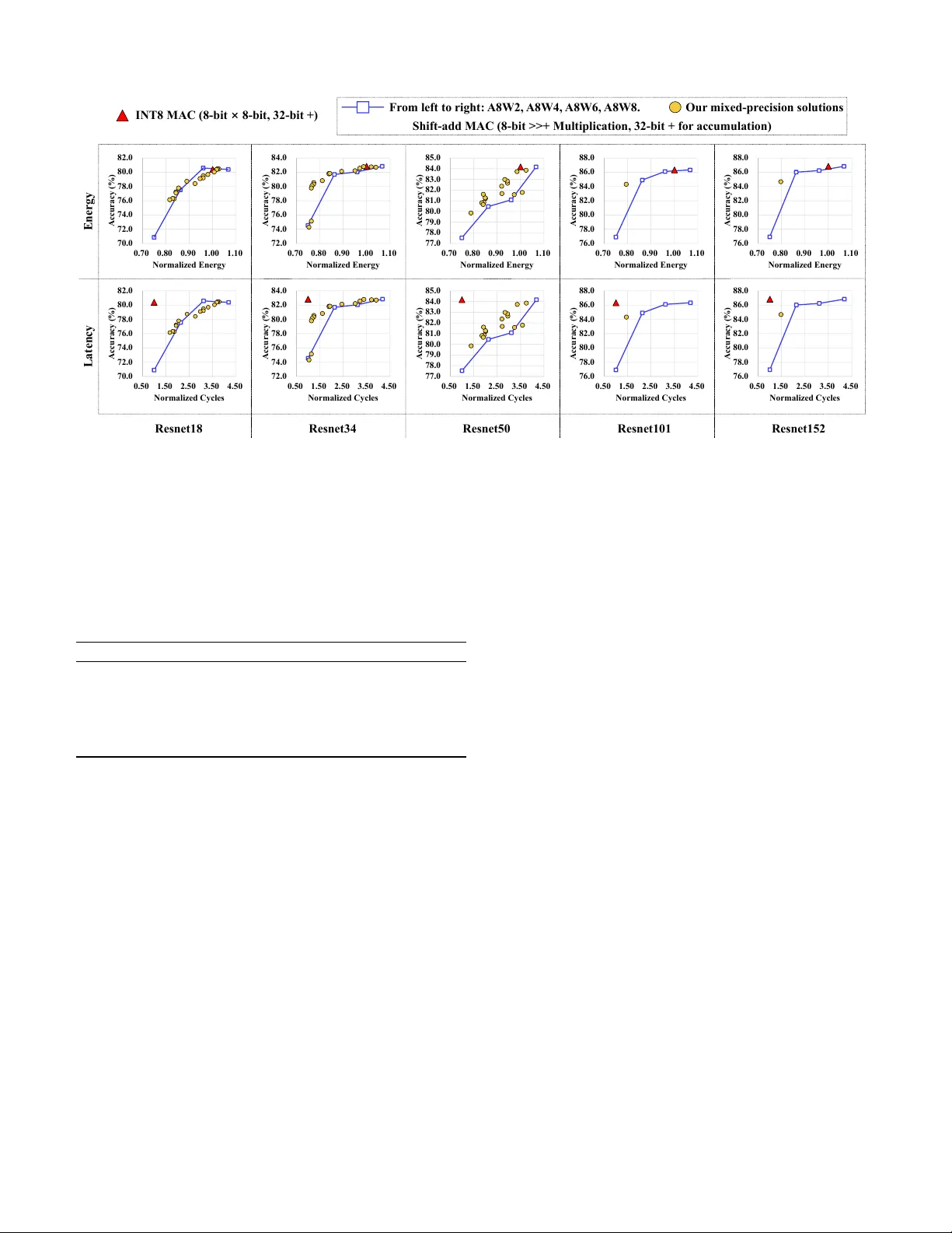
1 SigmaQuant: Hardware-A ware Heterogeneous Quantization Method for Edge DNN Inference Qunyou Liu ∗ , Pengbo Y u ∗ , Marina Zapater † , David Atienza ∗ , ∗ Embedded Systems Laboratory (ESL), EPFL, Switzerland, qunyou.liu@epﬂ.ch, pengbo.yu@epﬂ.ch, david.atienza@epﬂ.ch † University of Applied Sciences and Arts W estern Switzerland (HES-SO), Switzerland, marina.zapater@heig-vd.ch Abstract —Deep neural networks (DNNs) ar e essential f or performing advanced tasks on edge or mobile devices, yet their deployment is often hindered by sev ere r esource constraints, in- cluding limited memory , energy , and computational power . While uniform quantization provides a straightforward approach to compress model and reduce hardwar e r equirement, it fails to fully leverage the varying rob ustness acr oss layers, and often lead to accuracy degradation or suboptimal resour ce usage, particularly at low bitwidths. In contrast, heterogeneous quantization, which allocates different bitwidths to individual layers, can mitigate these drawbacks. Nonetheless, current heterogeneous quantiza- tion methods either needs huge brute-f orce design space sear ch or lacks the adaptability to meet different hardwar e conditions, such as memory size, energy budget, and latency requirement. Filling these gaps, this work introduces SigmaQuant , an adaptive layer -wise heterogeneous quantization framework designed to efﬁciently balance accuracy and resour ce usage f or varied edge en vironments without exhaustive search. SigmaQuant allocates layer -wise bitwidths based on weight standard de viation and KL diver gence, enabling adaptive quantization under real hardware constraints. This strategy efﬁciently balances accuracy , memory , and latency without the use of exhaustive search. W e validate its practicality through ASIC integration in a shift-add-based accelerator , analyzing power , performance, and ar ea (PP A) trade- offs f or the resulting mixed-pr ecision models. Experimentals on CIF AR-100 and ImageNet show that SigmaQuant consistently outperforms both uniform and state-of-the-art heter ogeneous quantization. At an equal size model, it achieves up to 2.0% higher accuracy; at an equal accuracy , it reduces memory by up to 40.0%. Hardwar e ev aluation demonstrates up to 22.3% area savings and 20.6% less energy cost compared to the widely used INT8 quantization and implementation, with slight latency overhead and comparable accuracy . These results conﬁrm the effectiveness of SigmaQuant for edge AI deployment. Index T erms —Hardwar e Accelerator , Neural Network, Algo- rithm, KL divergence I . I N T RO D U C T I O N Deep Neural Networks (DNNs) have become the backbone of many edge computing applications, ranging from image processing on devices [1] to speech recognition [2] and beyond. Howe ver , executing these models with strict resource budgets remains a formidable challenge. In particular , edge devices often have extremely limited memory size [3], [4], processing capabilities, and stringent energy supplies, which can make large and high-precision DNNs prohibiti vely expen- siv e or e ven infeasible to deploy [5], [6]. Quantization has emerged as one of the most effecti v e strategies to tackle this problem, as it con verts 32-bit ﬂoating point (FP) weights and acti vations into lower -precision repre- sentations (e.g., 8-bit or ev en 4-bit integers). This compression reduces the storage footprint and computational overhead of the model [7], [8]. Ho wev er , uniform quantization, where all layers share the same bitwidth, often fails to achie ve an optimal trade-off between accuracy and efﬁciency . The reason is that each DNN layer exhibits distinct statistical properties and different robustness to quantization noise [9], [10]. Therefore, forcing a single global precision can over - allocate bits to some layers and under-allocate them to others. T o overcome these limitations, heter og eneous quantization has recently gained popularity . This approach tailors the bitwidth per layer based on the quantization sensitivity of each layer , resulting in more compact models with minimal accuracy loss. Howe ver , existing methods typically rely on layer-wise sensitivity heuristics or resource-intensiv e search algorithms (e.g., reinforcement learning) [11], [12]. In addi- tion, edge devices exhibit various hardware conﬁgurations and resource constraints. For example, IoT sensors might hav e only a few me gabytes of available main memory , whereas mobile phones can offer signiﬁcantly more but require higher accuracy for applications like real-time image recognition or speech processing. Consequently , a static quantization scheme optimized for one scenario often fails to generalize to other hardware deployments. Formally , the quantization process should ideally satisfy boundary conditions on memory and accuracy constraints: Memory Usage ≤ Memory Constraint , Accuracy ≥ Accuracy Constraint . Current heterogeneous quantization methods fail to satisfy this adaptive requirement, as they typically provide ﬁxed solutions that cannot accommodate the diverse and dynamic demands of edge scenarios. Beyond algorithmic efﬁcienc y , heterogeneous quantization must also deliv er tangible hard- ware beneﬁts, particularly when deplo yed on edge AI accelera- tors. These accelerators increasingly rely on reduced-precision arithmetic to ef ﬁciently minimize area, power , and latenc y . The widely adopted shift-add scheme for multiply-accumulate (MA C) operations constitutes a representative example [13]– [16]. In such cases, lower bitwidths signiﬁcantly accelerate MA C computation, as fewer bits directly translate into less processing cycles and lower energy consumption. Howe ver , simply applying the lowest precision e v erywhere is ineffecti v e, since some layers are highly sensitive to quantization noise. Over -quantizing these layers can lead to se vere accuracy loss, undermining any hardware gains [17], [18]. This motiv ates a hardware-aware heterogeneous quantization strategy that carefully allocates precision across the network—assigning low bitwidths where feasible and preserving higher precision 2 where needed. Such an approach ensures compliance with hardware constraints (e.g., memory size, energy budgets, real- time latency) and maximizes the hardware ef ﬁciency . For this purpose, we propose SigmaQuant, a hardware- aware heterogeneous quantization framew ork that adaptiv ely allocates per-layer bitwidth under user-speciﬁed memory and accuracy targets, while fully leveraging hardware efﬁcienc y simultaneously . SigmaQuant has two search phases: (i) Phase- 1 provides a stable, constraint-aware initialization. All layers are grouped by simple distribution statistics so that the model quickly moves into a region that satisﬁes at least one boundary (memory size or accuracy). (ii) Phase-2 then performs ﬁne- grained adjustments on a fe w layers each time to meet both targets while a voiding unnecessary changes in most layers. The proposed two-phase scheme reduces the search ov erhead and effecti vely satisﬁes the requirements imposed by tight resource budgets. W e employ SigmaQuant on CIF AR-100 and ImageNet datasets and on a set of DNNs (e.g., ResNet and MobileNet) and compare performance with respect to a uniform quantization scheme and se veral state-of-the-art het- erogeneous quantization techniques. Furthermore, we ev aluate SigmaQuant on a general shift-add-based MA C unit widely used in modern edge accelerators, demonstrating its ef fecti ve- ness in reducing latenc y and ener gy . W e also provide a detailed trade-off analysis that highlights the co-optimization between software quantization strategies and hardware design, sho w- ing ho w SigmaQuant impacts performance, power , and area (PP A) metrics. This underscores the importance of proposing quantization methods that simultaneously optimize algorith- mic performance while adhering to hardware constraints for efﬁcient deployment. More speciﬁcally , the key contributions of our work are the follo wing: • W e introduce a distribution-based appr oach to study het- erogeneous quantization, fully utilizing the weight of each layer , guided by standard deviation and KL div ergence. • W e develop a two-phase quantization method that com- bines a cluster-based assignment with iterativ e div ergence- driv en reﬁnement, striking an effecti v e accuracy–ef ﬁciency balance in a reasonable design space search. Our method adapts the layer bitwidth assignments according to the user-deﬁned boundary conditions on accurac y and model size, ensuring minimal quantization loss while aggressiv ely compressing the network. • W e validate our method on CIF AR-100 [19] and Ima- geNet [20] with popular DNN architectures (mainly ResNet and MobileNet families). Compared to state-of-the-art het- erogeneous schemes, our approach (1) reduces memory usage by up to 17.7% while maintaining or exceeding accuracy and (2) reaches over 2% in T op-1 accurac y under similar memory budgets. Compared to uniform quantization, SigmaQuant can reach the same accuracy with only 60% memory budget, and achiev e 4% more accuracy with the same model size. • W e ev aluate SigmaQuant using a generic hardware im- plementation based on the shift-add scheme, which is widely used in edge scenarios. The results show that our method provides plenty of quantization choices between latency/ener gy and accuracy . It outperforms uniform quanti- zation schemes such as A8W4 in all metrics. Compared to a well-performing INT8 quantization strategy and hardware, SigmaQuant can further reduce area by 22.3% and energy consumption by up to 20. 6% with slight latency o verhead and comparable accuracy . The remainder of this paper is organized as follows. Sec- tion II describes the most relev ant heterogeneous quantization research in the state of the art. Section III explains the math- ematical e xplanation for the algorithm and hardware back- ground of suitable accelerator used in performance v alidation. Section IV details our distrib ution-ﬁtting approach and two- phase algorithm. Section V describes our experimental setup, followed by results and analysis in Section VI. W e conclude and discuss future directions in Section VII. I I . R E L A T E D W O R K Deep neural network quantization has seen e xtensiv e re- search to balance accuracy and efﬁciency for deployment on resource-constrained hardware. A common approach is uniform quantization, where all weights and activ ations are quantized to a ﬁxed bitwidth using a linear mapping scale. Uniform low-precision (e.g., 8-bit inte ger) models can signiﬁ- cantly reduce memory usage and speed up inference with only minor accuracy loss in many cases [11]. Howe ver , pushing uniform quantization to ultra-low bitwidths (4-bit or below) often incurs sev ere accurac y de gradation [11]. T echniques such as quantization-aware training and careful calibration improv e the situation [11], but ultimately a one-size-ﬁts-all bitwidth may not suit all layers. Some layers are more sensiti ve to quantization errors than others (as described in Section III-A), so using the same precision budget for ev ery layer can be suboptimal (as shown in Section VI-C). This rigidity motiv ates the use of adapti ve quantization strate gies. Non-uniform quantization techniques allocate quantization lev els une venly , guided by the sensiti vity of layers. Rather than spacing quantization lev els uniformly , these methods concen- trate precision where it matters the most (e.g., large-magnitude values). For instance, clustering or entropy-based schemes learn value clusters that maximize information content [21], effecti v ely compressing many small-magnitude weights into fewer le vels while reserving more lev els for important out- liers [21]. Zhu et al. propose an entropy-aw are layerwise quantization where the bitwidth of each layer is chosen based on the weight distribution entropy , allowing more complex layers to use higher precision (and vice versa) [22]. Baskin et al. [12] introduce a non-uniform k -quantile approach (UNIQ) that adapts the quantizer to the parameter distribution by injecting noise during training to emulate a quantile-based quantization. These non-uniform quantizers can better preserve accuracy under aggressiv e compression, especially in the lo w- bit regime [12], but their irregular quantization levels offer only a limited set of solutions and may not reliably meet memory constraints. Recent approaches formulate mixed-precision selection as an optimization problem under hardware constraints. Hardware-A ware Quantization framew orks like HA Q [23] 3 employ reinforcement learning to search for the Pareto-optimal bit allocation across layers gi ven a target memory or latency budget, automating mixed-precision selection. Its runtime depends on the training budget and on the details of the implementation. Lik ewise, differentiable Neural Architecture Search [24] techniques have been applied to quantization, learning per-layer precisions via gradient-based optimization [25], but this approach entails training a large super-netw ork (for bitwidth choices) – incurring considerable computational ov erhead – and can be sensitiv e to initialization and hyper- parameters. Second-order sensitivity analysis is also well established in statistics and machine learning [26], [27]. An alternativ e line of w ork uses second-order sensiti vity (HA WQ – Hessian-A W are Quantization). HA WQ lev erages the Hessian spectrum of each layer to gauge how quantization will impact the loss [27]. Heterogeneous DNNs have demonstrated that judiciously allocating higher bitwidth to error -sensiti ve layers and lower precision to tolerant layers can reduce model size and inference cost with only a small accuracy drop. There are also approaches for dynamic or adaptive precision at runtime. Instead of ﬁxing a mixed-precision conﬁguration post-training, a single model is trained to support multiple bitwidth settings. Jin et al. [28] propose AdaBits, which enables a network to switch between bitwidths on the ﬂy (e.g., 2-bit to 8-bit) without retraining. By joint training with adaptive bitwidths and using techniques like switchable clipping le vels for acti vations, they obtain a model that can cater to dif ferent hardware capabilities or energy budgets. This adds a new dimension of ﬂexibility: one deployed model can adapt to v arious scenarios. The trade-of f is a more in volv ed training procedure (to ensure the network performs well at all supported precisions) and a slight runtime overhead to manage precision switching. Existing network quantization methods, including uniform and mixed-precision approaches, often do not explicitly min- imize the diver gence between the pre- and post-quantization distributions of weights or acti vations. Instead, the y use in- direct criteria (e.g. minimizing quantization noise variance or heuristics lik e entropy/KL to set ranges), which do not guarantee that the quantized v alues preserve the original distribution [29]. This oversight can lead to a mismatch in distributions that degrades accuracy , as recently noted by sev eral studies [29] [30]. Moreov er , most quantization frame- works produce a ﬁxed precision conﬁguration for a model. Many mixed-precision techniques explore only a handful of bitwidth assignments and then adopt a static scheme, which lacks ﬂexibility across different hardware settings [31]. This nature means the model cannot easily adapt its bitwidth per layer to meet the constraints or capabilities of new devices. In summary , earlier quantization methods did not explicitly align distributions and often yielded ﬁxed precision setups. While heterogeneous quantization effecti vely tailors preci- sion to each layer’ s tolerance, deployment on real hardware demands further consideration. Edge AI accelerators, whether ASIC, DSIP , DSP , FPGA, etc., operate under strict area, po wer , and latency constraints. Reduced-precision arithmetic directly affects all these metrics, as lo wering bitwidth reduces MA C complexity , diminishes the memory footprint and data move- ment, and thereby decreases power consumption. For example, for the shift-add scheme widely used in many accelerators, each additional bit in a multiplier operand contrib utes an extra cycle and corresponding po wer cost. Thus, lowering the weight bitwidth yields an approximately proportional reduction in compute latency and energy consumption per operation. Howe ver , nai vely pushing all layers to the lowest precision can dev astate accuracy , since sensitiv e layers quickly lose accuracy under o ver -quantization. Existing quantization techniques largely ne glect this co-optimization. Many prior methods focus on accuracy and model size (often via heuristic or search-based bit allocations) without e xplicitly modeling hardware costs. These approaches yield ﬁxed precision as- signments that may satisfy a bit-budget or tar get accuracy but run afoul of practical limits like on-chip memory capacity , power budgets, or throughput constraints. In other w ords, a model might be well-compressed in theory but still too slow or energy-hungry for the target hardware. This gap in prior work motiv ates a hardware-a ware solution that jointly addresses algorithmic and hardware objectiv es. Beyond early mixed- precision schemes such as HA Q and HA WQ, recent work has progressed along sev eral complementary directions that explicitly consider hardware constraints and/or more e xpres- siv e search formulations. On the hardware–software co-design side, Edge-MPQ [32] integrates versatile mixed-precision in- ference units into a RISC-V pipeline and couples them with a hardware-aw are layer-wise MPQ search, targeting latency and energy on a speciﬁc edge platform. On the training/sensiti vity side, Huang et al. [33] propose HMQA T , a Hessian-based mixed-precision QA T framework that dri ves bit conﬁguration via a Pareto-frontier search and further improv es stability through transition-aware ﬁne-tuning of quantization scales. From the perspecti ve of joint compression under an accelerator objectiv e, Balaskas et al. [34] e xplore a combined pruning– quantization design space with a reinforcement-learning agent guided by an accelerator -lev el ener gy model. Finally , Deng et al. [35] present CLADO, which e xplicitly models cross-layer dependencies of quantization errors and formulates bitwidth assignment as an integer quadratic program to obtain strong accuracy–compression trade-offs. Motiv ated by these adv ances and their practical trade-of fs, our proposed approach, SigmaQuant , adopts a lightweight yet hardware-aw are distrib ution-ﬁtting perspecti ve for heteroge- neous quantization. Speciﬁcally , SigmaQuant uses layer -wise standard de viation and the KL di ver gence between the ﬂoating- point and quantized distributions to guide bitwidth assignment in a two-phase procedure that enforces user -deﬁned accuracy and resource constraints (model size or BOPs) without e x- haustiv e search, while remaining compatible with integer-only shift-add accelerators. I I I . B A C K G RO U N D In this section, we ﬁrst revie w the con v entional (uniform) quantization scheme and then introduce our perspectiv e of approximating each layer’ s weight distrib ution by a discrete (quantized) distribution. This distribution-ﬁtting viewpoint motiv ates why different layers may require distinct bitwidths. 4 W e also highlight the increasing importance of hardware- constrained design, wherein bitwidth choices must align with metrics such as model size to meet resource and latency tar gets on edge devices, and we provide some background on the speciﬁc hardware design that we use to sho wcase the results of our work. A. Model Quantization and Distribution 1) Uniform Quantization Basics.: Let w ∈ R n denote the set of weights in a given DNN layer . In a uniform quantization scheme with inte ger bitwidth b , each weight w i is replaced by a quantized value ˜ w i = clip  round  w i ∆  , − Q, Q  × ∆ , where Q = 2 ( b − 1) − 1 (for signed quantization) and ∆ is the quantization step size (or scale). T ypically , ∆ is chosen in one of two ways: • Max-based scaling , where ∆ = max i | w i | /Q , • Statistical scaling , where ∆ = k σ , with σ denoting the standard de viation of w (and k a chosen constant, e.g., 2 or 3 ). All weights are thus mapped to one of 2 b uniformly spaced lev- els in [ − Q ∆ , Q ∆] . While straightforward, a global uniform bitwidth can be suboptimal because different layers exhibit widely v arying sensiti vities to quantization noise [11], [12], [27], [36]. This observation motiv ates heter og eneous quanti- zation , wherein each layer (or channel) is allo wed its o wn bitwidth b ℓ . Such layer-wise customization yields better ac- curacy–size trade-offs: for example, early con volutional layers often hav e smaller weight v ariance and can safely be quantized to 4 bits, whereas layers with broader weight distributions may require 8 bits to retain accuracy . The challenge, then, is to determine how to assign precision across layers in a principled yet efﬁcient way . 2) Quantization Sensitivity and Standar d Deviation: W e conducted preliminary experiments to identify a simple indica- tor of layer-wise quantization sensitivity . Using ImageNet [20] as dataset and Alexnet [37] and ResNet18 [38] as example models, we applied progressiv ely lower bitwidths per layer to reach minimum Bits Operations (BOPs) [12] under a ﬁxed ov erall precision budget using brute-force search. A remarkably strong correlation emer ged between each layer’ s acceptable bitwidth and the standard de viation σ ( Sigma ) of its weights: layers with relatively lo w σ tolerated very lo w precision (4-bit or even 2-bit) with minimal accuracy impact, whereas layers with high σ either needed to remain at higher precision (e.g., 8-bit) or suf fered severe accuracy drops when forced to fe wer bits. T able I illustrates this trend for AlexNet running on ImageNet, where an initial heuristic assignment (uniform 8-bit for all layers) is compared against the ﬁnal adjusted bitwidths. Layers with larger σ (e.g., Conv1 ) ended up requiring higher b ℓ to av oid excessiv e quantization error , as reﬂected by the lar ger KL div ergence D K L between the original and quantized weight distributions for those layers. In contrast, layers with small σ (e.g., the fully-connected layers) were quantized to 2 bits with negligible D K L penalty . ResNet18 shows the same trend. T ABLE I O B SE RV A T IO N S O N A BA S E L IN E ( BO P - BA S E D ) H E UR I S T IC V S . FI N AL B I TW I D T H A N D W E I G HT D I ST R I BU T I O N F O R A L EX N E T ( I MA G E N E T ) . H I GH E R S TA ND AR D D EV I A T I ON σ C O R RE L A T E S W I TH T H E N E ED F O R H I GH E R B I T WI D T H T O K E E P T H E K L D IV E R G EN C E D K L L OW . Layer Init Bits Final Bits σ D K L AlexNet – Conv1 8 6 0.115672 0.022229 AlexNet – Conv2 8 6 0.046543 0.000626 AlexNet – Conv3 8 4 0.034646 0.000477 AlexNet – Conv4 8 4 0.027320 0.000409 AlexNet – Conv5 8 4 0.026128 0.000619 AlexNet – FC1 8 2 0.009245 0.000097 AlexNet – FC2 8 2 0.011537 0.000104 AlexNet – FC3 8 4 0.018524 0.000136 These empirical ﬁndings conﬁrm that the weight standard deviation σ ℓ is a strong ﬁrst-order indicator of layer ℓ ’ s quan- tization sensiti vity . Intuiti vely , σ ℓ gauges the “width” of the weight distrib ution: a large spread means more information can be lost when mapping to a small set of le vels, whereas a tightly concentrated distribution can be compressed more aggres- siv ely . This insight aligns with prior observations that layer- wise weight distributions inﬂuence quantization outcomes. For instance, the quantization whitepaper in [9] recommends setting the quantizer range based on multiples of the weight standard de viation, and Zhu et al. propose an entropy-based bit allocation per layer to account for distrib ution comple xity [22]. More sophisticated frame works have also quantiﬁed layer sensitivity via reinforcement learning or second-order analysis (Hessian) [11], reinforcing the notion that certain layers are inherently more error-prone under quantization. Our results show that a simple statistic σ ℓ can serv e as an effecti ve proxy for this sensitivity , pro viding a con venient starting point for assigning heterogeneous bitwidths. In practice, this means we can sort or cluster layers by σ ℓ and assign lo wer precisions to those with small σ ℓ while reserving higher bits for layers with large σ ℓ , before applying an y ﬁne-grained adjustments. 3) Distribution-F itting P erspective .: While σ provides a useful heuristic, we also adopt a theoretical perspectiv e to quantify quantization loss more rigorously . Consider the em- pirical distribution of the weights in layer ℓ , denoted p ℓ ( w ) . W e can write p ℓ ( w ) = 1 | W ℓ | X w i ∈ W ℓ δ ( w − w i ) , where W ℓ = { w i } is the set of weights and δ ( · ) is the Dirac delta (this can be thought of as the normalized weight histogram for layer ℓ ). After quantizing layer ℓ to b ℓ bits, the set of quantized weights { ˜ w i } induces a discrete distribution ˜ p ℓ ( w ) supported only on the ﬁnite quantization lev els. Rather than vie wing quantization merely as per-weight rounding error , we regard it as an information-theor etic appr oximation of p ℓ by ˜ p ℓ . A natural measure of the mismatch between these two distributions is the Kullback–Leibler (KL) div ergence: D K L  p ℓ ∥ ˜ p ℓ  = X w p ℓ ( w ) log p ℓ ( w ) ˜ p ℓ ( w ) . (1) When the quantization step size (represented by b l ) is too small compared to the range of values in W l , the quantized 5 representation ˜ p l will not capture the differences between many distinct v alues, leading to a loss of precision. Con versely , a suf ﬁciently high b ℓ yields ˜ p ℓ that closely approximates p ℓ , resulting in a small KL div ergence. In essence, choosing an appropriate bitwidth b ℓ amounts to balancing model size (or ef- ﬁciency) against an acceptable le vel of distribution distortion. This distribution-ﬁtting vie w provides a theoretical foundation for quantization: one seeks to minimize information loss by ensuring ˜ p ℓ is a good ﬁt to p ℓ . Importantly , this perspectiv e helps explain the earlier em- pirical trend with σ ℓ . A layer with a large σ ℓ typically has a broad p ℓ ( w ) ; quantizing it aggressi vely (small b ℓ ) forces a poor approximation ˜ p ℓ ( w ) , yielding a high D K L and, ultimately , higher accuracy degradation. In contrast, a layer with small σ ℓ (narrow distribution) can be quantized to lo w precision with only a minor increase in D K L . In practice, we le verage D K L as a quantiﬁcation of quantization “distortion” to complement the σ ℓ heuristic. Recent studies similarly note that preserving the original distrib ution (or minimizing distribution shift) is critical for maintaining accuracy [39]. Thus, by using σ ℓ as a ﬁrst-order guide and D K L ( p ℓ ∥ ˜ p ℓ ) as a reﬁnement criterion, we ground our heterogeneous quantization strategy in both empirical intuition and theoretical approximation. Subsequent sections will reference these metrics as the basis for our two-phase bitwidth assignment algorithm, without needing to repeat the justiﬁcation for why the y are chosen. B. Exploiting SigmaQuant in Efﬁcient shift-add-based Accel- erators for Edge Devices M u ltip lican d X = 0. 9296875 0 1 1 0 1 0 0 0 × M u ltip lier Y = 0. 875 0 1 1 1 = ( 0. 8125, ↓ 0. 12% ) + X * 1 + 0 X * 1 + > > 0 X * 0 = 0 1 1 1 0 1 1 1 AI M o d els ( a) Ar ith m et ic o f AI ( b ) M u ltip licatio n b y s h if t - ad d iter atio n s + > > 1 X * 1 > > 1 C onv G EMM Mu l t . Ad d Sh if t ∑ Acc. (b ) Fig. 1. (a) The operation hierarchy of AI models from top to down, and (b) the widely used shift-add-based multiplier for edge accelerators that target at high energy efﬁcienc y . Modern edge and mobile devices are constrained by limited memory , computational power , and energy resources, which signiﬁcantly hampers DNN inference on these platforms. T o increase the speed-up and efﬁcienc y of inference in resource- constrained platforms, models are quantized and executed on dedicated or domain-speciﬁc hardware accelerators. The core computation behind DNNs are matrix multi- plications (GEMMs) and conv olutions, both of which are fundamentally composed by MA C operations, as presented in Figure 1(a). Consequently , enhancing the efﬁciency of multi- plication and accumulation is crucial. In this conte xt, shift-add- based multipliers [13]–[16] are widely employed in hardware accelerators, as they can reduce area consumption, lo wer power costs, and relax critical timing constraints. Figure 1(b) illustrates an example of an 8-bit × 4-bit multiplication, yielding an 8-bit result via iterativ e shift-add operations. The input operands are in Q1.X format, that 1-bit for integer (i.e., 0 or -1) and others for fraction, ranging in (-1,1). The process begins at the least signiﬁcant bit (LSB) of the multiplier, with each bit processed sequentially through an addition follo wed by a right-shift, and concludes at the most signiﬁcant bit (MSB). The multiplication result is truncated to 8 bits, that is the same size of the multiplicand, since truncation loss is often minimal (only -0.12% in this example). Howe v er , while the shift–and-add scheme offers signiﬁcant area and energy efﬁciency , it is constrained by increased la- tency , as a naive implementation requires n-cycle iterations for an n-bit multiplier operand. Consequently , reducing the size of the multiplier operand can substantially impro ve latency performance and further enhance energy efﬁcienc y . Although techniques such as executing multiple shift operations for trailing zeros (e.g., “1000”) within a single cycle [16], [40] or employing Canonical Signed Digit (CSD, e.g., 0111 to 100-) coding [16] for the multiplier hav e been proposed to mitigate this issue, the overall latenc y remains strongly correlated with the size of the multiplier operand. For DNNs, the multiplier operand typically corresponds to the weight. Therefore, using lower -bitwidth weights can eliminate latency concerns while simultaneously yielding additional reductions in energy consumption. Therefore, in this work, we target a generic shift-add based arithmetic scheme to assess the beneﬁts of our pro- posed quantization method relati ve to uniform quantization baselines, with the ev aluation reﬂecting arithmetic efﬁcienc y rather than being bound to any particular hardware platform. More detailed discussion about model size, latenc y , energy consumption are provided in Section-VI. I V . M E T H O D O L O G Y A. Algorithm Overview Based on our preliminary experiments and observations, SigmaQuant proposes a two-phase procedure to determine per-layer quantization bitwidths, focusing ﬁrst on a coarse clustering assignment and then on ﬁne-grained adjustments. The goal of this section is to explain the structure and logic of this algorithm (summarized in Algorithm 1) without delving into lo w-lev el implementation or mathematical deri v ations. W e take adv antage of two k ey metrics – weight standard deviation (Sigma) and Kullback–Leibler (KL) div ergence – to guide decisions (see Section III-A for the mathematical foundation and preliminary experiments results of these metrics). In essence, Phase 1 provides an initial clustering-based bitwidth assignment, and Phase 2 provides an iterativ e, div ergence- based reﬁnement. Throughout the procedure, the algorithm tracks the accuracy and size of the model relativ e to these targets (with some buffer tolerance, ∆ A for accuracy and ∆ M 6 for size) and uses two key metrics to guide decisions: weight standard deviation (denoted σ , a measure of the spread of the distribution of a layer) and Kullback-Leibler (KL) diver - gence between the original and quantized weight distributions. Algorithm 1 outlines the overall procedure at a high level, summarizing the two phases described belo w . 1) Phase 1 - Initial Phase (Cluster-Based Bitwidth As- signment): The algorithm clusters the layers based on standard deviation σ using an adapti ve k -means method (with penalty parameter λ ). Each cluster is mapped to a target bitwidth (e.g., from the set { 2 , 4 , 6 , 8 } ). After quan- tization and calibration, the model’ s accuracy and size are compared against the desired targets (with buf fers ∆ A and ∆ M ). If neither metric is acceptable, the clustering is reﬁned (by increasing λ ) and the process repeats until at least one metric meets its boundary . 2) Phase 2 - Reﬁnement Phase (Iterative Improv ement): The algorithm ﬁne-tunes the bitwidths of individual lay- ers. A sensitivity score—combining σ and the KL div er- gence between the full-precision and quantized weight distributions—is computed for each layer . Layers with high sensiti vity (i.e., those most critical to accurac y) are adjusted by increasing their bitwidth, while layers with low sensitivity may have their bitwidth reduced to save memory . This iterativ e reﬁnement continues until both accuracy and model size meet the targets, thereby placing the model in the T arget Zone. Fig. 2. Ov erview of our proposed distribution-ﬁtting quantization method. W e start from user-deﬁned boundary conditions (target model size and accuracy) and adapt bitwidths in two phases: initial clustering by standard deviation followed by iterativ e KL-based reﬁnement. Figure 2 illustrates this two-phase procedure on a plot of model accurac y (y-axis) versus model size (x-axis). In the diagram, color-coded regions indicate the algorithm’ s decision zones. W e preserve those visual cues here to e xplain how the algorithm navigates the accuracy–model size trade-of f: • Bit Increase Zone (Phase 1 light green region): The model’ s accurac y is too low , yet its current size is com- fortably below the target budget. In this scenario, accuracy is the bottleneck. The algorithm responds by increasing bitwidths for certain layers (typically those most sensiti ve to quantization error) to regain accuracy • Bit Decrease Zone (Phase 1 light red region): The model’ s accuracy is acceptable (at or above the required threshold), but the model size exceeds the target memory budget. Here, efﬁcienc y is the problem. The algorithm decreases bitwidths for some less-sensitiv e layers to compress the model and reduce its size • T ransition Zone (middle gray-green region): Continue the previous cluster trend until reaching the next zone. • Abandon Zone (gray region): Neither accuracy nor model size is anywhere near acceptable lev els. In this rare case, the procedure may terminate early to avoid wasting resources on a hopeless quantization scenario (i.e., the chosen constraints might be unattainable simultaneously). T erminate process. • Iteration Zone (Phase 2 region): This zone represents the intermediate state where one of the two criteria (accuracy or size) has met its target, but the other one has not yet met it. The model stays in this zone during the Phase 2 reﬁnement process. The algorithm will perform iterati ve bitwidth tweaks – increasing or decreasing precision for selectiv e layers – to improve the remaining metric while maintaining the already satisﬁed metric, effecti vely nudging the model tow ard the T arget Zone. • T arget Zone (light orange region): Both accuracy and model size meet their target thresholds (within the allowed buf fers). When the model lands in this zone, it means it satisﬁes the accuracy requirement and does not exceed the size budget. B. Phase 1: Adaptive Clustering In the ﬁrst phase, we assign initial bitwidths to each layer by clustering their standard deviations into K = 4 groups, targeting for the bitwidths of 2-, 4-, 6-, 8-bit. For the initia assignment, we use the conv entional k-mean. Then we check the location of the initial point in the Fig. 2, before we decide to increase the bitwidth or decrease the bitwidth. Next, unlike standard k -means, we introduce a adapti ve term that discourages certain cluster from becoming too large, thus promoting a more uniform distribution of layers across the av ailable bitwidths. Concretely , let X = { x 1 , x 2 , . . . , x N } be the set of N layers we wish to cluster , where x i is a one- dimensional feature (e.g. standard deviation σ i ). W e seek a partition C = { C 1 , C 2 , . . . , C K } , of X into K clusters. W e deﬁne the centroid of C j as µ j = 1 | C j | X x ∈ C j x. The adaptive k -means objectiv e reads min C , µ j K X j =1  X x ∈ C j ∥ x − µ j ∥ 2 + λ  | C j | − N K  2  , (2) where λ controls ho w strongly we penalize de viations from the “ideal” cluster size N K . For each iteration: • W e compute the distances from each layer x i to the centroid of each cluster , adjusted by the cluster-size penalty term λ . 7 Algorithm 1 T wo-Phase Heterogeneous Quantization Require: Float model M with N layers; v alid bit-set B = { 2 , 4 , 6 , 8 } ; targets A t , M t ; tolerances ∆ A, ∆ M ; max iters I max Ensure: Quantised model M q 1: M q ← Initialize8Bit ( M ) ▷ start with uniform 8-bit 2: A ← Evaluate ( M q ) 3: M ← ModelSize ( M q ) — Phase 1: adaptiv e clustering — 4: λ ← 0 . 1 ; i ← 0 5: while ( A < A t − ∆ A ) ∧ ( M > M t + ∆ M ) ∧ ( i < I max ) do 6: i ← i + 1 7: feat ← StdDevFeatures ( M q ) 8: C ← AdaptiveKMeans ( feat , 4 , λ ) 9: AssignBitwidths ( C , M q , B ) 10: Calibrate ( M q ) ; QA T ( M q ) 11: A ← Evaluate ( M q ) ; M ← ModelSize ( M q ) 12: if ( A ≥ A t − ∆ A ) ∨ ( M ≤ M t + ∆ M ) then 13: br eak ▷ one metric is inside the buffer 14: else 15: λ ← λ + 0 . 1 16: end if 17: end while 18: if ( A < A t − ∆ A ) ∧ ( M > M t + ∆ M ) then 19: retur n M q ▷ gi ve up – infeasible 20: end if — Phase 2: iterativ e reﬁnement — 21: j ← 0 22: while j < I max do 23: j ← j + 1 24: Improv eBitwidths ( M q ) 25: Calibrate ( M q ) ; QA T ( M q ) 26: A ← Evaluate ( M q ) ; M ← ModelSize ( M q ) 27: if ( A ≥ A t ) ∧ ( M ≤ M t ) then 28: br eak 29: end if 30: end while 31: retur n M q • W e reassign x i to the cluster that minimizes its total cost. • W e update the centroids µ j after all points are reassigned. W e initialize λ to a small value (e.g., 0 . 1 ) and gradually increase it (in increments, such as 0 . 1 ) whene ver the resulting bitwidth assignment fails to meet either of the global buf fer conditions ( ∆ A and ∆ M in 1). Each time a new clustering C is obtained, we map each cluster C j to a target bitwidth b j ∈ { 2 , 4 , 6 , 8 } . W e then calibrate and perform a short quantization-aware training (QA T) cycle. If neither accurac y nor model size usage falls within the acceptable range, we increment λ and repeat. If, after a ﬁxed maximum number of increments, both metrics remain unacceptably far from their targets, the algorithm halts (“abandoning” the attempt and announcing the failure of quantization). W e perform a quick calibration of the quantized model before QA T by using a subset of training data to adjust batchnorm statistics and quantization scales (ensuring stable QA T initialization). C. Phase 2: Iter ative KL-Based Reﬁnement Once Phase 1 ensures that at least one of the tar get con- straints (accuracy or model sizes) is satisﬁed, we proceed to a ﬁner-grained iterativ e improv ement of the per-layer bitwidths. Here, we focus on adjusting bitwidths to ﬁx whichever metric remains suboptimal. W e deﬁne a sensiti vity measure for each layer ℓ that combines its standard deviation and a normal- ized Kullback–Leibler (KL) di ver gence between the ﬂoat and quantized weight distributions. W e use the KL di ver gence as described in Equation 1. W e use a normalized version b D KL to bound it between 0 and 1, e.g. by di viding by D KL  p ℓ ∥ p int8  for an 8-bit baseline distribution p int8 . In each iteration of Phase 2 we perform the follo wing actions: 1) Measure Sensitivity: For layer ℓ , we deﬁne a sensitivity score b D KL ( p ℓ ∥ ˜ p ℓ ) , Layers with a higher b D KL are more critical to accuracy , so if accuracy is below the target, we increase their bitwidth ﬁrst. Con versely , if model size usage is too high, we decr ease bitwidth on layers with a lower sensiti vity score. 2) Apply Changes & Calibrate: W e pick a small number of layers (e.g., 2 or 3) to adjust by ± 2 bits (within the allow able range { 2 , 4 , 6 , 8 } ). W e then recalibrate and run a short QA T cycle. 3) Re-Evaluate Metrics: W e check the global accuracy and model size usage. If both are within their b uffers, we stop; if neither is acceptable, we keep adjusting. 4) Early Stopping / Rev ersion: If too many consecuti ve adjustments fail to mov e the metrics closer to their goals, we revert to the previous stable assignment and exit. W e use symmetric min–max range quantization for weights, performed per output channel (as implemented in Brevi- tas [41]), which is a common hardware-friendly scheme. For activ ations, we adopt asymmetric quantization with statistical clipping at the 99.9th percentile to reduce outlier sensitivity and improve calibration rob ustness. Unless stated otherwise, we follow a memory-centric objective (Model Size counted on weights only), and thus keep activ ations ﬁxed at 8 bits while allowing layer-wise weight bitwidths to v ary within { 2 , 4 , 6 , 8 } under SigmaQuant; when targeting compute (BOPs), both weights and activ ations can be adapted with the same pro- cedure. Compared to recent MPQ methods that (i) co-design precision assignment with platform-speciﬁc inference units and pipelines (e.g., Edge-MPQ [32]), (ii) rely on second-order sensitivity (Hessian) and specialized transition-aware QA T (e.g., HMQA T [33]), (iii) explore a joint pruning–quantization space via reinforcement learning with an accelerator-le v el energy model [34], or (iv) formulate bitwidth assignment as a global inte ger quadratic program with cross-layer de- pendency modeling (e.g., CLADO [35]), SigmaQuant adopts a lightweight distribution-ﬁtting strategy . More speciﬁcally , Phase 1 clusters layers using σ for a stable near-feasible initialization, and Phase 2 uses KL div ergence to mak e small local bitwidth updates that explicitly enforce user-deﬁned ac- curacy and resource constraints, without platform-speciﬁc co- design, Hessian estimation, RL exploration, or IQP solvers. By iterating this local adjustment approach, Phase 2 ensures that the model con verges smoothly to a conﬁguration that respects both accuracy and model size constraints without introducing large distrib utional mismatches at once; in practice, this step often accounts for relatively few bitwidth changes, giv en that Phase 1 has already established a near-feasible starting point. 8 V . E X P E R I M E N T A L S E T U P T o validate the effecti veness of SigmaQuant we conduct ex- periments on ImageNet [42] and CIF AR-100 datasets [43] us- ing InceptionV3 [44] and ﬁ ve standard ResNet v ariants [45]— ResNet18, ResNet34, ResNet50, ResNet101, and ResNet152. W e e valuate the proposed approach against state-of-the-art heter og eneous quantization approaches as well as con ven- tional uniform quantization methods. T o compare the result with other state-of-art method, we run experiments using the ImageNet (See Sec. VI-B). T o show the trend and relation between the model size and accuracy , we run an experiment using CIF AR-100 to sa ve GPU resources (see Sec. VI-C). W e acquire the full-precision pre-trained models from the pytorch ofﬁcial website [46] for ImageNet. For CIF AR-100, we train these models again ourselves on the target dataset before quantization using either: • Unif orm Quantization: All layers share a ﬁxed bitwidth (e.g., 2, 4 or 8 bits). • SigmaQuant (Ours): Layers receive bitwidths guided by their weight distribution properties (standard deviation and optional diver gence checks). Before quantization, a short calibration phase (using a small subset of the training set) is performed. Then QA T is used to mitigate performance degradation. The metrics used to assess the different techniques are the following: 1) Model Size (MB): Sum of quantized weights across all layers. 2) T op-1 Accuracy (%): Evaluated on the CIF AR-100 test set. 3) Regression Analysis: For combined sets of quantized models, we ﬁt accuracy–model-size curves and plot error bands (standard deviation) to visualize overall trends. Moreov er , to validate the hardware impact from Sig- maQuant , we map the Resnet family on a general shift-add- based MAC unit and ev aluate the latency and po wer consump- tion information through post-synthesis simulation with TSMC 28nm library . Our e xperiments were run on NVIDIA A100 and V100 GPUs, and the results were validated through more than 8’500 GPU hours. V I . R E S U L T S In this section, we ﬁrst illustrate how the quantization process ev olv es over time in our two-phase algorithm, high- lighting the transition from cluster-based assignment to it- erativ e reﬁnement. Then, we compare the performance of our method against state-of-the-art heterogeneous quantiza- tion schemes. Next, we analyze the trade-off between model size and accuracy in CIF AR-100, providing information on resource-accuracy balance. In the following, we discuss the hyperparameter ef fect. Finally , we demonstrate the potential hardware advantages. A. Phase-Based Learning Pr ocess T o illustrate the dynamic process of our method, we track the quantization states (”start” to ”end”) of a representati ve model (e.g., ResNet34) as it progresses through the two-phase algorithm described in Section IV. Figure 3 plots the model accuracy (in %) against the corrected model sizes (in megabyte), depicting the iterative exploration of the bit incr ease , bit decr ease , and tar get regions: • Start Point – Con ventional Clustering: Initially , the bitwidth assignment is based on k-means clustering of layers. This coarse clustering provides an initial bitwidth assignment that quickly improves accuracy while causing the model size to approach the target buffer ( Fig. 3 left). • Phase I – Iterati ve Re-Clustering: In Phase I, the model re-clusters individual layer bitwidths using an adapti ve clus- tering method (Eq. 2). This technique assigns bitwidths to a higher or lower cluster , transitioning the model from the bit- increasing zone to the bit-decreasing zone and subsequently into Phase 2 (Fig. 3 middle). • Con ver gence and Abort Conditions: Once one of the tar get metrics (accuracy or model size) meets the b uffer threshold, Phase 2 commences. Here, we compute a sensitivity score for each layer that combines its weight standard deviation with a normalized Kullback–Leibler diver gence measure. Layers exhibiting minimal di ver gence, indicating that further precision reduction would incur only minor accuracy loss, are selectively adjusted (Fig. 3 right). W e ﬁx the number of clusters to 4, corresponding to weight bitwidths of { 2 , 4 , 6 , 8 } -bit. These choices are illustrativ e, and other conﬁgurations could equally be adopted. Phase 1 runs up to 2 iterations (this number can be conﬁgured to a higher value when f acing larger models), each followed by 4 epochs of QA T . Phase 2 allows up to 40 reﬁnement steps with 40 QA T epochs per step, adjusting 2 layers (we ﬁxed this to 2 layers in our implementation for all experiments) per iteration based on sensitivity . QA T uses cross-entropy loss and SGD (for ResNet) or Adam (for others), with a reduced learning rate. W e start from INT8 quantized models. The accuracy threshold is set to 1% drop, and the memory constraint targets 75% of the INT8 model size ( ≈ 18.75% of the FP32 baseline). In general, Figure 3 demonstrates the stability of the quantization path, showing that only a handful of iterations are typically required before a near-optimal trade-off between accuracy and model size overhead. Additionally , we compare the conﬁguration obtained after Phase I alone with the ﬁnal conﬁguration after Phases I–II, to quantify the added beneﬁt of Phase II. T able II summarizes results across models under a ≤ 2% accuracy-drop constraint and a ≤ 40% INT8-size budget. As noted, Phase 1—our fast, adaptive k-means clustering based solely on layer-wise standard deviation—can leav e the model slightly abov e or below the memory tar get; the table therefore reports the Phase 1 (“std-only”) accuracy/size alongside the ﬁnal result after Phase 2. After Phase 1 we choose a direction: either increase the bitwidth of the most sensitiv e layers to recover accuracy or decrease bitwidths where possible to meet the size budget. This operating region near 35–40% of the INT8 size is particularly challenging because further bitwidth reductions leav e limited headroom to preserve accurac y . For ResNet-18, Phase 1 already satisﬁes the size budget but the accuracy drop is e xcessi ve; increasing the precision of selected layers ( ↑ in 9 Fig. 3. Example showing how training advances through the two-phase quantization for ResNet34. The x-axis represents corrected model sizes and the y-axis represents model accuracy . Different points indicate successiv e stages in the cluster phase (Phase 1) and iteration phase ((Phase 2), with the ﬁnal quantized model landing in the target area. T ABLE II M O DE L S IZ E S A N D A CC U R AC I ES . Model Int8 Size (MiB) Int8 Acc. (%) Final Acc. (%) Final Size (MiB) Phase I Acc. (%) Phase I Size (MiB) Next Phase T arget Meet ResNet18 11.14 80.40 78.41 3.72 75.98 3.20 ↑ ✓ ResNet34 20.77 82.90 - - 81.14 6.52 - ✓ ResNet50 24.32 84.01 81.21 8.49 82.57 8.93 ↓ ✗ ResNet101 42.38 85.98 84.31 12.28 84.78 15.26 ↓ ✓ ResNet152 57.26 86.77 84.67 16.72 85.26 22.66 ↓ ✗ T able II) restores accuracy while keeping the model within budget, so both constraints are ultimately met. F or ResNet-34, both constraints are met after Phase 1, so no reﬁnement is required. For ResNet-50, the size tar get is met but the accurac y constraint remains violated e ven after Phase 2, indicating that the two targets cannot be satisﬁed simultaneously under this setting. B. P erformance Comparisons with State-of-the-Art Heter oge- neous Quantization Schemes In this subsection, we compare our proposed quantization technique ( Ours ) against state-of-the-art methods on ResNet- 50 [38] and InceptionV3 [44], focusing on model size (in MB) and T op-1 accuracy (%). W e implement our method to achieve optimal performance under v arious memory constraints by setting target bitwidths to 2, 4, 6, and 8, resulting in a mixed-bitwidth conﬁguration. T able III consolidates results from prior work [11], [12], [35], [36], [47]–[49] alongside our heterogeneous bitwidth assignments for weights (W) and activ ations (A) (column Bits(W ,A) in the table). W e emphasize weight precision while treating activ ations as 8-bit, since our primary objectiv e is memory reduction. For each model, we list the baseline full-precision size and accuracy , then compare uniform or mixed-precision baselines to illustrate how different bit conﬁgurations trade off memory and accu- racy . The methods labeled Ours highlight tw o representativ e conﬁgurations that demonstrate a fa v orable balance between model compactness and classiﬁcation performance. T ABLE III C O MPA R IS O N O F Q UA N T I ZAT IO N M E T H OD S O N I N CE P T I ON V 3 A N D R E S N E T - 5 0 . Method Bits(W ,A) Model Size(MB) T op-1 Acc.(%) ResNet-50 Baseline [11] 32,32 97.8 77.72 Apprentice [36] 2+, 8+ 14.11 72.8 UNIQ [12] 4,8 12.8 74.37 UNIQ [12] 4+, 8+ 12.8 75.1 Apprentice [36] 4+, 8+ 20 74.7 Apprentice [36] 2+,32 14.1 74.7 UNIQ [12] 4,32 12.8 75.09 HA WQ-V3 [11] 8,8 24.5 77.58 HA WQ-V3 [11] 4/8,4/8 18.7 76.73 HA WQ-V3 [11] 4,4 13.1 74.24 CLADO [35] mix, 8 17.89 75.42 CLADO [35] mix, 8 13.42 73.10 Ours mix,8 12.02 76.86 Ours mix,8 10.78 75.63 InceptionV3 Baseline [11] 32,32 90.9 78.88 Integer Only [8] 8, 8 22.7 74.20 Integer Only [8] 7, 7 20.1 73.70 R VQuant [12] 8,8 22.7 74.22 HA WQ-V3 [11] 4/8,4/8 19.6 74.65 Ours mix,8 19.63 74.73 Focusing primarily on memory ef ﬁciency , these results sho w that our heterogeneous quantization yields models that are up to 7–10 × smaller than the full-precision baseline, while retaining most of the original accuracy . For example, for ResNet-50, Ours (mix,8) (12.02 MB) exceeds 76% accuracy , aligning with methods that use similar or slightly larger model sizes, while 13.1MB for HA WQ-V3 with 74.24% accuracy , 13.42MB for CLADO with 73.10% accurac y . Similarly , for In- ceptionV3, our method reach similar Model Size (19.6MB for HA WQ-V3, 19.63MB for Ours) and T op-1 accuracy (74.65% 10 for HA WQ-V3, 74.73% for Ours) as the HA WQ-V3. Notably , we achie ve these gains using a straightforward procedure that incorporates standard deviation and diver gence metrics to adapt the bitwidth per layer . Compare to the HA WQ- V3, our method support more bitwidths choices, and it can shrink the model size adapti vely according to the memory constrain (as shown in Fig.4(b)). These comparisons conﬁrm that our method ef fecti vely balances memory footprint with competitiv e accuracy , making it a suitable choice for scenarios where model size is the foremost constraint. In our design, SigmaQuant’ s search cost is dominated by short QA T loops rather than by an expensi ve discrete search. Phase 1 computes per-layer statistics (one scalar σ per layer) and runs adaptiv e k -means on these L layers with K = 4 clusters, which is limited in practice (M iterations for example). Computing KL div ergences uses layer histograms and scales with the number of parameters P once per reﬁnement round. Phase 2 mak es small local moves—changing m layers per round ( m = 2 in our setup)—and applies brief QA T to re-stabilize accuracy . Overall, the wall-clock is therefore well approximated by the number of QA T epochs: Cost ≈  M E P1 + N E P2  × T epoch , where M is the number of phase 1 rounds, E P1 are Phase 1 epochs, N is the number of reﬁnement rounds, E P2 are epochs per round, and T epoch is the time for one QA T epoch. In our experiments we cap Phase 1 at normally 1 to 3 iterations and Phase 2 runs normally within 5 (smaller models) to 40 (large models) reﬁnement rounds, with early stopping once both accurac y and size targets are met. As a result, end-to- end times are model-dependent: for the runs in this paper we measured ≈ 2 to 30 hours for ResNet-18/34/50/101/152, respectiv ely , using A100/V100 GPUs (see Sect. VI-C). W e do not claim to be faster than calibration-only PTQ meth- ods that av oid any ﬁne-tuning; instead, SigmaQuant trades a moderate ofﬂine search for two properties that those methods typically lack: (i) hard-constraint adapti vity (meeting user- speciﬁed accuracy/size targets across devices) and (ii) con- sistently better accuracy–size and hardware PP A trade-of fs (T ables II III, Figs. 4). Methods such as HA WQ-V3 estimate per-layer sensitivity via second-order information and solve a global assignment with ILP; their runtime is dominated by many backward passes for Hessian/spectrum estimation plus calibration, after which assignment is relativ ely cheap. UNIQ and Apprentice require training (noise injection or distillation) across multiple epochs; they do not perform a per -layer mixed- precision search but still incur substantial wall-clock due to full-model optimization. SigmaQuant lies in between: it av oids Hessian estimation and global RL/ILP search, yet it still adapts layer preci- sions to explicit hardware/accuracy constraints via a small number of targeted QA T loops. In short, SigmaQuant is not a “zero-search” PTQ method; it is an adaptiv e mix ed- precision method with linear-in-layers bookkeeping and a bounded number of short QA T epochs, which empirically yields fav orable accuracy–size–hardware trade-of fs under tight device constraints. C. Model Size and Accuracy Analysis Another key advantage of our method is its adaptiv e nature. By dynamically adjusting the boundary conditions for both the model size buf fer and the accurac y target, our approach performs layer-wise quantization in a highly ﬂexible man- ner , a capability that pre vious methods lack. Figure 4 (a) compares model size and T op-1 accuracy on CIF AR-100 for ﬁv e different ResNet architectures (ResNet-18, ResNet-34, ResNet-50, ResNet-101, and ResNet-152) under two quan- tization schemes: conv entional uniform quantization and our SigmaQuant approach. Across all model variants, SigmaQuant (plotted as darker markers) achie ves higher accuracy for a giv en model size than their uniformly quantized counterparts (lighter markers). In practical terms, for an equal memory footprint, a model quantized with SigmaQuant yields 4% more accuracy . F or the same accuracy , the model size can shrink by around 40%. Notably , the uniform quantization approach is unable to reach the optimal balance between model size and accuracy , highlighting its inherent limitations. This trend holds consistent as networks become deeper: model quantized with our method surpasses the accurac y of a similarly-sized uniformly quantized one. For e xample, the ResNet50 sigma can achieve similar accuracy (81.0% for uniform quantiza- tion, 81.7% for sigma quantization) with better model size (18.24MB for uniform quantization, 13.98MB for sigma quan- tization). In ef fect, SigmaQuant retains and, in some cases ev en improv es, the predictive performance while aggressi vely reducing the size of the model. T o further illustrate the overall trend, Fig. 4 (b) consolidates the results by plotting top-1 accuracy against model size for all quantized ResNet models tested, with linear regression ﬁts for each quantization scheme (sigma-based vs. uniform) and shaded ±1 σ error bands. The key observ ation is that the ﬁtted curve for SigmaQuant lies consistently abo ve that of uniform quantization across the entire range. The separation between these trendlines is substantial, and the error bands show minimal ov erlap, indicating that the accuracy gap is statistically robust across multiple runs. In other words, Sig- maQuant achie ves a gi ven accuracy le vel with fewer parame- ters (3.2MB Model Size Saving in Fig. 4 (b)), or con versely , for the same number of parameters (same memory b udget), it deliv ers higher accuracy than uniform precision (4% Accuracy Gain in Fig. 4 (b)). This translates to a more fav orable accuracy–ef ﬁciency trade-off. Notably , the advantage becomes ev en more pronounced for larger models: SigmaQuant ’ s accu- racy approaches that of higher-precision (e.g., 32-bit) networks at a fraction of the memory usage as model size grows. Such behavior is highly desirable for resource-constrained deploy- ments, as it means that one can enjoy near -baseline accuracy without the cost of a large model. Overall, the regression ﬁts and non-overlapping error bands indicate that SigmaQuant consistently provides a better accuracy–model-size trade-off than uniform quantization across different ResNet depths. Our experiments also demonstrate that SigmaQuant remains practical for ofﬂine training across the ResNet family . For example, under an extreme constraint, limiting the model size to achie ve at least 25% memory savings while tolerating at 11 Fig. 4. (a) Comparison of T op-1 accuracy versus model size for various ResNet architectures on CIF AR-100, where darker markers denote the sigma -based method and lighter markers denote uniform quantization. (b) Regression ﬁts with ±1 σ error bands reveal that the sigma approach consistently achiev es higher accuracy at equiv alent model sizes. most 1% accuracy drop relativ e to the full precision model, the total quantization search and training times were approxi- mately 4, 2, 1.5, 5.5, and 26 hours for ResNet-18, ResNet- 34, ResNet-50, ResNet-101, and ResNet-152, respectively . These runtimes remain within a reasonable range for ofﬂine deployment. Even in cases where the training process fails due to ov erly tight memory constraints, we observe from the generated models that SigmaQuant still produces meaningful accuracy–ef ﬁciency trade-of fs, as shown in the corresponding ev aluation ﬁgures. D. Hyperparameter and the Activation W e study the impact of the accuracy/size buf fers (∆ A , ∆ M ) and the reﬁnement schedule (max rounds N max , step size m layers/round, and QA T epochs/round E P2 ) on con ver gence and wall-clock. Recall that Phase 1 ends once either of the metrics enters its buf fer (Alg. 1, lines 12–16), whereas Phase 2 continues until both strict targets are met (lines 27–31). Thus, larger b uffers generally reduce Phase 1 iterations but may require more Phase 2 reﬁnements; smaller buffers hav e the opposite effect. W e keep K =4 clusters and the default 2-layer step in Phase 2 unless otherwise stated. T able IV summarizes typical behavior on ResNet-34/CIF AR-100 under our default targets (at most 1% accuracy drop), varying only (∆ M ) and reﬁnement settings. The trends hold qualitati vely for other models. Overall, smaller buf fers ( Conservative ) reduce the chance of overshooting a target but increase observed rounds N and wall-clock; larger buf fers ( Aggr essive ) do the opposite, at a slight risk of needing extra micro-adjustments later in Phase 2. In all cases, the ﬁnal solution respects the strict tar gets due to the Phase 2 stopping rule. Moreov er , except the weights for the memory saving, we adapt the activ ation to reduce the amount of BOPs. T o ev aluate activ ation reduction fairly , we switch the target from memory to compute: BOPs ≜ P ℓ B w ( ℓ ) B a ( ℓ ) MACs( ℓ ) , T ABLE IV S E NS I T I VI T Y O F S I G M A Q U AN T O N R E S N E T - 3 4 ( C I FAR - 1 00 ) U N DE R T HE D E F AU LT TAR G E T S . Numbers shown ar e placeholders. Setting ∆ A ∆ M Obs. M Obs. N T ime (h) Meet? Conservati ve 1% 85% 3 0 ∼ 4.5 ✓ Balanced (default) 1% 75% 3 3 ∼ 12.6 ✓ Aggressiv e 1% 50% 4 5 ∼ 19.0 ✗ where the B w ( ℓ ) and B a ( ℓ ) are the bitwidth of weight and activ ation; MA Cs is the multiply–accumulate operation of this layer . It upper-bounds bit-le vel work and correlates with ener gy/latency (on our shift-and-add MA Cs, cycles scale primarily with B w ) while exposing the beneﬁt of lower - ing B a . W e then run SigmaQuant with a compute bud- get (BOPs) and an accurac y tar get, letting both weights and acti vations adapt. T able V reports indicati ve results on AlexNet/ResNet-18/ResNet-32/ResNet-50 on CIF AR-100 with a 1% accuracy-drop target and a 25–35% BOPs-reduction budget. As expected, acti vation down-quantization reduces BOPs but lea ves Model Size (MB) unchanged; SigmaQuant co-adapts layerwise weights to maintain accuracy . When the optimization target is memory (weight size), changing acti- vation bitwidth has no ef fect on Model Size (MB) because activ ations are not counted in that metric. Under a compute target (BOPs), SigmaQuant naturally co-optimizes to ward lower activ ation precision while preserving accuracy , yielding 35–50% BOPs reductions in our indicati ve runs with ≤ 2.5% accuracy loss. T ABLE V A C T I V ATI O N R E D U CT I O N U N DE R A B O P TA RG E T . Model ∆ A ∆ BOP ResNet-18 78.91% ( − 32 . 9% ) ResNet-34 81.31% ( − 49 . 4% ) ResNet-50 82.38% ( − 32 . 0% ) 12 7 6 . 0 7 8 . 0 8 0 . 0 8 2 . 0 8 4 . 0 8 6 . 0 8 8 . 0 0. 70 0. 80 0. 90 1. 00 1. 10 A ccu ra cy ( % ) N o rma l i z ed E n erg y 7 6 . 0 7 8 . 0 8 0 . 0 8 2 . 0 8 4 . 0 8 6 . 0 8 8 . 0 0. 70 0. 80 0. 90 1. 00 1. 10 A ccu ra cy ( % ) N o rma l i z ed E n erg y 7 0 . 0 7 2 . 0 7 4 . 0 7 6 . 0 7 8 . 0 8 0 . 0 8 2 . 0 0. 70 0. 80 0. 90 1. 00 1. 10 A ccu ra cy ( % ) N o rma l i z ed E n erg y 7 2 . 0 7 4 . 0 7 6 . 0 7 8 . 0 8 0 . 0 8 2 . 0 8 4 . 0 0. 70 0. 80 0. 90 1. 00 1. 10 A ccu ra cy ( % ) N o rma l i z ed E n erg y 7 7 . 0 7 8 . 0 7 9 . 0 8 0 . 0 8 1 . 0 8 2 . 0 8 3 . 0 8 4 . 0 8 5 . 0 0. 70 0. 80 0. 90 1. 00 1. 10 A ccu ra cy ( % ) N o rma l i z ed E n erg y R e s ne t18 R e s ne t34 R e s ne t50 R e s ne t101 R e s ne t152 Shi ft - add M A C (8 - bi t > > + M ul ti pl i c ati on, 32 - bi t + for ac c um ul ati on) I NT 8 M AC ( 8 - bi t × 8 - bi t, 32 - b it +) F r om l e ft to r i ght: A 8W 2, A 8W 4, A 8W 6, A 8W 8. O ur m i xe d - pr e c i si on sol uti ons 7 6 . 0 7 8 . 0 8 0 . 0 8 2 . 0 8 4 . 0 8 6 . 0 8 8 . 0 0. 50 1. 50 2. 50 3. 50 4. 50 A ccu ra cy ( % ) N o rma l i z ed C y cl es 7 6 . 0 7 8 . 0 8 0 . 0 8 2 . 0 8 4 . 0 8 6 . 0 8 8 . 0 0. 50 1. 50 2. 50 3. 50 4. 50 A ccu ra cy ( % ) N o rma l i z ed C y cl es 7 0 . 0 7 2 . 0 7 4 . 0 7 6 . 0 7 8 . 0 8 0 . 0 8 2 . 0 0. 50 1. 50 2. 50 3. 50 4. 50 A ccu ra cy ( % ) N o rma l i z ed C y cl es 7 2 . 0 7 4 . 0 7 6 . 0 7 8 . 0 8 0 . 0 8 2 . 0 8 4 . 0 0. 50 1. 50 2. 50 3. 50 4. 50 A ccu ra cy ( % ) N o rma l i z ed C y cl es 7 7 . 0 7 8 . 0 7 9 . 0 8 0 . 0 8 1 . 0 8 2 . 0 8 3 . 0 8 4 . 0 8 5 . 0 0. 50 1. 50 2. 50 3. 50 4. 50 A ccu ra cy ( % ) N o rma l i z ed C y cl es En erg y La t en cy Fig. 5. Normalized energy consumption (top) and cycle count (hence latency , bottom) versus accuracy for all ResNet models with uniform quantization(A8W2, A8W4, A8W6, A8W8) and sigma quantization schemes. An INT8 MA C, which has 1-cycle 8-bit × 8-bit multiplier and 32-bit adder , is used as a baseline for performance comparison. FP32, FP16, and BF16 alternati ves are not presented here since they incurs huge overhead , that up to 5.5 × , 4.0 × , and 3.6 × more energy cost. All the data are normalized with INT8 computation. The closer a dot element is to the top-left corner, the better its performance and accuracy . T ABLE VI M AC I M P L EM E N T A T I ON S FP32 FP16 BF16 INT8 Shift-add Multiplication 32-bit 1 subword FP32 × 32-bit 2 subwords FP16 × 32-bit 2 subwords BF16 × 32-bit 4 subwords INT8 × 32-bit 4 subwords 8-bit ≫ + Accumulation 1 subword FP32 + 2 subwords FP32 + 2 subwords FP32 + 4 subwords INT32 + 4 subwords INT32 + Area / µ m 2 3218.3 3837.9 3501.9 2103.4 1635.4 Overall, these results sho w that our distribution-guided Sig- maQuant method provides an effecti ve balance between model compression and predictiv e performance. By judiciously allo- cating bitwidths based on per-layer weight statistics and distri- butional di ver gence, SigmaQuant consistently produces more compact models without sacriﬁcing accuracy under the same model-size constraints. This represents a compelling improve- ment over uniform quantization, making our approach well- suited for real-world DNN deployment in memory-limited embedded environments. E. Hardwar e P erformance Analysis A key advantage of heterogeneous quantization is that it lev erages the varying robustness of different layers to maintain accuracy while allo wing the corresponding hardw are to oper- ate with less area occupation, fe wer c ycle count, and lower energy consumption, increasing all beneﬁts. In this work, we target a widely used shift-add MA C implementation to ev aluate the performance under different quantization schemes. This MAC unit has an 8-bit shift-add- based multiplier that supports 8 -bit × n -bit → 8 -bit multipli- cation through iterativ e right-shift and addition, followed by a 32-bit adder for accumulation. The shift-add design performs a single addition and multiple right-shift operations within each cycle, which enables to process trailing zeros of the multiplier operand, reducing the average latency to roughly n/2 cycles for an n-bit operand. The shift-add MA C hardware is implemented in TSMC 28nm technology (0.9V , 600MHz) and features a 32-bit datapath. It should be emphasized that the arithmetic performance comparison reﬂect a general case applicable to all technology nodes and hardware platforms, while the presented implementation is intended primarily for illustrativ e purposes. W e also implemented FP32, FP16, BF16, and INT8 alternativ es under the same conditions, detailed in T able VI. It can be found that shit-add MAC implemen- tation reduces 22.3% area over the INT8 one, and more than 49.2% over others. W e characterize the performance using post-synthesis simulation, mapping all con volutional and fully-connected layers of ResNet models onto the hardware. The energy consumption and cycle count for inference are ev aluated, as shown in Figure 5. In Figure 5, we sho w the normalized energy consumption (top, a) and cycle count (hence latency , (bottom, b)) of different quantization schemes across benchmarks. Both our SigmaQuant scheme and the uniform quantization approach are mapped on the shift-add design, whereas the typical INT8 quantization is performed with the INT8 hardware that already has high ef ﬁciency . The results of FP32, FP16, BF16 are not included, since they incur up to 5.5 × , 4.0 × , and 3.6 × more energy cost over the INT8 one, respecti vely . The uniform quantization approach has 13 four combinations of 8-bit acti v ations and 2/4/6/8-bit weights, namely as A8W8, A8W6, A8W4 and A8W2. All the v alues are normalized by the INT8 MA C implementation. The accuracy drop is deﬁned as the dif ference between FP32 reference and the quantized ones. As expected, in uniform quantization, when weights reduce from 8-bit to 4-bit, and especially to 2-bit, the accuracy dramatically drops. T aking Resnet34 as an example, ev en if uniform quantization A8W2 sav es 25.0% energy consumption wrt. the INT8 case, it de grades accuracy by 8.54%. Howe ver , SigmaQuant performs a larger search in the design space and is able to address this issue, achieving 23.3% energy savings ov er the INT8 alternati ve with only a 2.97% accuracy loss. As for the A8W4 case, uniform quantization can save 13.8% ener gy consumption with 1.39% accuracy loss while our method reduces 16.0% energy cost with only 1.25% accuracy degradation. Furthermore, the results of SigmaQuant are consistent across all the benchmarks, always yielding data points located closer to the upper left corner in the ﬁgure wrt. the uniform approach, hence less latency and energy consumption with lo wer accuracy loss. The only exception is ResNet18, where SigmaQuant sho ws a very similar trend to uniform quantization, since such model is too small and therefore the space search is limited. Still, SigmaQuant can get 15.7 % less ener gy consumption wrt. the INT8 case with 3.76% accuracy drop while that of uniform quantized one is 13.8% and 3.45%. For larger models such as Resnet101 and Resenet152, that provides enough searching space, our SigmaQuant method can reduce up to 20.6% and 20.3% energy cost wrt. the INT8 alternati ve, which is already a well-known solution, with comparable accuracy . Note that the model size of our method is always smaller than that of INT8 quantization for all the comparisons. Similar trend can be observed in the latency performance. Due to the serial shift-add-based multiplication, even multiple shifts per cycle is used, it still incurs latency overhead. For e xample, the A8W8 uniform quantization of ResNet34, runs 4.2 × slo wer than the INT8 case. Thanks to the fully exploitation and optimization by SigmaQuant , howe ver , it dramatically cuts this overhead. F or Resnet34, it lowers ener gy by 23.3% while increasing latency by only 17.5% relative to the INT8 alternative. This analysis only considers the general shift-add arithmetic, yet the advantages would become far more pronounced with speciﬁc techniques such as CSD encoding [16] applied to the multiplier operand. In addition, uniform quantization of fers a very limited range of choices, making it difﬁcult to balance accuracy with latency and ener gy efﬁcienc y . In contrast, the SigmaQuant dot distrib ution shown in Figure 5 illustrates a broader set of quantized models. For example, the options between A8W2 to A8W4 or A8W4 to A8W6 for ResNet18, ResNet34, and ResNet50. This greater ﬂexibility allows for more effecti ve tailoring to div erse hardware requirements, including model size, runtime latency , and energy budget. Overall, these results demonstrate that distrib ution-guided, layer-wise bit allocation can signiﬁcantly enhance hardware efﬁcienc y compared to uniform quantization. In fact, our approach sho ws greater improv ements than the A8W4 v ari- ant, approaching the ef ﬁciency of A8W2 quantization while incurring minimal accuracy loss, and can further improv e hardware ef ﬁciency than typical INT8 solution. As model size decreases, ﬁne-grained quantization leverages the shift- add architecture to achie ve lower latency and reduced power consumption, offering a compelling solution for resource- constrained deployments. V I I . C O N C L U S I O N In this work, we have presented SigmaQuant , an adaptive, layerwise heterogeneous quantization framew ork that lever - ages a distribution-ﬁtting approach to assign bitwidths based on both weight standard deviation and KL diver gence. Our two-phase method, featuring an initial cluster -based bitwidth assignment follo wed by an iterativ e, div ergence-dri v en reﬁne- ment, ef fecti vely balances accuracy and model size with a reasonable searching effort, ensuring that quantized models maintain high performance while achieving signiﬁcant com- pression. A key strength of SigmaQuant is its inherent adapt- ability . Across different platforms with varying constraints and requirements, our framew ork consistently adapts bit al- location to satisfy speciﬁc resource budgets. For example, by integrating with hardware-centric metrics such as model size and target accuracy , SigmaQuant directly translates per-layer quantization decisions into efﬁcient bitwidth assignments that align with the overall requirements of the system. In general, our e xperimental results on CIF AR-100 and ImageNet across multiple DNN architectures demonstrate that SigmaQuant not only outperforms state-of-the-art heterogeneous quanti- zation and uniform quantization, but also provides a robust and hardware-a ware solution for ef ﬁcient DNN inference in resource-limited environments. Furthermore, experiments on general hardw are arithmetic scheme validate our results from both po wer and latency perspectives, further emphasizing the advantages of our approach. This adapti ve, dynamic method pav es the way for the practical deployment of deep neural networks in a wide range of embedded systems. V I I I . A C K N O W L E D G M E N T S This work w as supported in part by the Swiss State Secre- tariat for Education, Research, and Innovation (SERI) through the SwissChips research project, and also by Intel as part of the Intel Center for Heterogeneous Integrated Platforms (HIP). R E F E R E N C E S [1] A. Krizhevsky , I. Sutskever , and G. E. Hinton, “Imagenet classiﬁcation with deep convolutional neural networks, ” Commun. A CM , v ol. 60, no. 6, p. 84–90, May 2017. [Online]. A vailable: https://doi.org/10.1145/ 3065386 [2] D. Amodei et al. , “Deep speech 2: end-to-end speech recognition in english and mandarin, ” in Proceedings of the 33rd International Confer ence on International Conference on Machine Learning - V olume 48 , ser. ICML ’16. JMLR.org, 2016, p. 173–182. [3] Q. Liu, M. Zapater, and D. Atienza, “MatrixFlow: System–accelerator co-design for high-performance transformer applications, ” arXiv pr eprint arXi v:2503.05290, 2025. [Online]. A v ailable: https://arxiv .org/ abs/2503.05290 [4] ——, “Gem5-AcceSys: Enabling system-le vel exploration of standard interconnects for novel accelerators, ” arXiv preprint 2025. [Online]. A v ailable: https://arxiv .org/abs/2502.12273 [5] V . Sze, Y .-H. Chen, T .-J. Y ang, and J. S. Emer , “Efﬁcient processing of deep neural networks: A tutorial and surve y , ” Proceedings of the IEEE , vol. 105, no. 12, pp. 2295–2329, 2017. 14 [6] L. Deng, “Model compression and acceleration for deep neural net- works: The principles, progress, and challenges, ” IEEE Signal Process- ing Magazine , vol. 37, no. 6, pp. 101–110, 2020. [7] S. Han, H. Mao, and W . J. Dally , “Deep compression: Compressing deep neural networks with pruning, trained quantization and huffman coding, ” in International Conference on Learning Repr esentations (ICLR) , 2016. [8] B. Jacob, S. Kligys, B. Chen, M. Zhu, M. T ang, A. Howard, H. Adam, and D. Kalenichenko, “Quantization and training of neural networks for efﬁcient integer-arithmetic-only inference, ” Proceedings of the IEEE Confer ence on Computer V ision and P attern Recognition (CVPR) , pp. 2704–2713, 2018. [9] R. Krishnamoorthi, “Quantizing deep conv olutional networks for efﬁ- cient inference: A whitepaper, ” 2018. [10] R. Banner, I. Hubara, E. Hoffer , and D. Soudry , “Scalable methods for 8-bit training of neural networks, ” Advances in Neural Information Pr ocessing Systems (NeurIPS) , vol. 31, pp. 5145–5153, 2018. [11] Z. Y ao, Z. Dong, Z. Zheng, A. Gholami, J. Y u, E. T an, L. W ang, Q. Huang, Y . W ang, M. W . Mahoney , and K. K eutzer , “Hawq-v3: Dyadic neural network quantization, ” in Pr oceedings of the 38th International Confer ence on Machine Learning . PMLR, 2021, pp. 11 875–11 886. [12] C. Baskin, E. Schwartz, E. Zheltonozhskii, N. Liss, R. Giryes, A. M. Bronstein, and A. Mendelson, “Uniq: Uniform noise injection for non-uniform quantization of neural networks, ” A CM Tr ansactions on Computer Systems , vol. 37, no. 1–4, pp. 1–15, 2021. [13] P . Judd, J. Albericio, T . Hetherington, T . M. Aamodt, and A. Moshovos, “Stripes: Bit-serial deep neural network computing, ” in 2016 49th Annual IEEE/ACM International Symposium on Microar chitectur e (MI- CR O) . IEEE, 2016, pp. 1–12. [14] L.-C. Hsu, C.-T . Chiu, K.-T . Lin, H.-H. Chou, and Y .-Y . Pu, “Essa: An energy-aw are bit-serial streaming deep conv olutional neural network accelerator , ” Journal of Systems Architectur e , vol. 111, p. 101831, 2020. [15] M. Rios, F . Ponzina, A. Levisse, G. Ansaloni, and D. Atienza, “Bit-line computing for cnn accelerators co-design in edge ai inference, ” IEEE T ransactions on Emerging T opics in Computing , vol. 11, no. 2, pp. 358– 372, 2023. [16] P . Y u, F . Ponzina, A. Le visse, M. Gupta, D. Biswas, G. Ansaloni, D. Atienza, and F . Catthoor, “ An ener gy efﬁcient soft simd microar- chitecture and its application on quantized cnns, ” IEEE T ransactions on V ery Large Scale Inte gration (VLSI) Systems , 2024. [17] Z. Dong, Z. Y ao, A. Gholami, M. W . Mahoney , and K. K eutzer , “HA WQ: Hessian aw are quantization of neural networks with mixed precision, ” in Proc. IEEE/CVF Int’l Conf. Computer V ision (ICCV) , 2019. [18] A. Y azdanbakhsh, A. T . Elthakeb, P . Pilligundla, F . S. Mireshghallah, and H. Esmaeilzadeh, “ReLeQ: A reinforcement learning approach for deep quantization of neural networks, ” , 2019. [19] A. Krizhevsk y and G. Hinton, “Learning multiple layers of features from tiny images, ” 2009, technical Report. [20] O. Russakovsk y , J. Deng, H. Su, J. Krause, S. Satheesh, S. Ma, Z. Huang, A. Karpathy , A. Khosla, M. Bernstein et al. , “Imagenet large scale visual recognition challenge, ” International Journal of Computer V ision , vol. 115, no. 3, pp. 211–252, 2015. [21] E. Park, J. Ahn, and S. Y oo, “W eighted-entropy-based quantization for deep neural networks, ” in 2017 IEEE Confer ence on Computer V ision and P attern Recognition (CVPR) , 2017, pp. 7197–7205. [22] X. Zhu, Q. Li, and D. W ang, “Entropy-based layerwise quantization for efﬁcient deep neural networks, ” in Pr oceedings of the IEEE Conference on Computer V ision and P attern Recognition . IEEE, 2018, pp. 1234– 1243. [23] K. W ang, Z. Liu, Y . Lin, J. Lin, and S. Han, “Haq: Hardware-aw are automated quantization with mixed precision, ” in 2019 IEEE/CVF Confer ence on Computer V ision and P attern Recognition (CVPR) , 2019, pp. 8604–8612. [24] T . Elsken, J. H. Metzen, and F . Hutter, “Neural architecture search: a survey , ” J. Mach. Learn. Res. , vol. 20, no. 1, p. 1997–2017, Jan. 2019. [25] B. Wu, X. Dai, P . Zhang, Y . W ang, F . Sun, Y . Wu, Y . Tian, P . V ajda, Y . Jia, and K. Keutzer , “Fbnet: Hardware-aware efﬁcient convnet design via differentiable neural architecture search, ” 2019 IEEE/CVF Confer ence on Computer V ision and P attern Recognition (CVPR) , pp. 10 726–10 734, 2018. [Online]. A vailable: https://api.semanticscholar . org/CorpusID:54461508 [26] H. Cai, M. F . Kaloorazi, and J. Chen, “Online generalized eigenvectors extraction via a ﬁxed-point approach, ” IEEE Tr ansactions on Signal Pr ocessing , vol. 69, pp. 2435–2451, 2021. [27] Z. Dong, Z. Y ao, D. Arfeen, A. Gholami, M. W . Mahoney , and K. Keutzer , “Hawq-v2: Hessian aw are trace-weighted quantization of neural networks, ” in Advances in Neural Information Processing Systems , H. Larochelle, M. Ranzato, R. Hadsell, M. Balcan, and H. Lin, Eds., vol. 33. Curran Associates, Inc., 2020, pp. 18 518– 18 529. [Online]. A v ailable: https://proceedings.neurips.cc/paper ﬁles/ paper/2020/ﬁle/d77c703536718b95308130ff2e5cf9ee- P aper .pdf [28] L. W ang and B. Chen, “ Adabits: Adaptiv e bitwidth quantization for deep neural networks, ” in Pr oceedings of the IEEE Conference on Computer V ision and P attern Recognition . IEEE, 2020, pp. 5560–5568. [29] A. Finkelstein, U. Almog, and M. Grobman, “Fighting quantization bias with bias, ” ArXiv , vol. abs/1906.03193, 2019. [Online]. A vailable: https://api.semanticscholar .org/CorpusID:174801144 [30] C. Hong and K. M. Lee, “Overcoming distribution mismatch in quantizing image super-resolution networks, ” 2024. [Online]. A vailable: https://openrevie w .net/forum?id=GOt2kP383R [31] A. Bulat and G. Tzimiropoulos, “ Bit-Mixer: Mixed-precision networks with runtime bit-width selection , ” in 2021 IEEE/CVF International Confer ence on Computer V ision (ICCV) . Los Alamitos, CA, USA: IEEE Computer Society , Oct. 2021, pp. 5168–5177. [Online]. A vailable: https://doi.ieeecomputersociety .or g/10.1109/ICCV48922.2021.00514 [32] X. Zhao, R. Xu, Y . Gao, V . V erma, M. R. Stan, and X. Guo, “Edge- MPQ: Layer-wise mixed-precision quantization with tightly integrated versatile inference units for edge computing, ” IEEE T r ansactions on Computers , vol. 73, no. 11, pp. 2504–2519, 2024. [33] Z. Huang, X. Han, Z. Y u, Y . Zhao, M. Hou, and S. Hu, “Hessian-based mixed-precision quantization with transition aware training for neural networks, ” Neural Networks , vol. 182, p. 106910, 2025. [34] K. Balaskas, A. Karatzas, C. Sad, K. Siozios, I. Anagnostopoulos, G. Zervakis, and J. Henkel, “Hardware-aware DNN compression via div erse pruning and mixed-precision quantization, ” IEEE T ransactions on Emerging T opics in Computing , vol. 12, no. 4, pp. 1079–1092, 2024. [35] Z. Deng, S. Sharify , X. W ang, and M. Orshansky , “Mixed-precision quantization for deep vision models with integer quadratic program- ming, ” in Proceedings of the 62nd ACM/IEEE Design Automation Confer ence (D AC) , 2025, pp. 1–7. [36] A. Mishra and D. Marr, “ Apprentice: Using knowledge distillation techniques to improv e low-precision network accuracy , ” in International Confer ence on Learning Representations (ICLR) , 2018. [37] A. Krizhevsky , I. Sutskever , and G. E. Hinton, “Imagenet classiﬁcation with deep con volutional neural networks, ” in Advances in Neural Infor- mation Processing Systems , 2012, pp. 1097–1105. [38] K. He, X. Zhang, S. Ren, and J. Sun, “Deep residual learning for image recognition, ” in Pr oceedings of the IEEE Confer ence on Computer V ision and P attern Recognition , 2016, pp. 770–778. [39] M. Federici, R. T omioka, and P . Forr ´ e, “ An information-theoretic ap- proach to distribution shifts, ” in Pr oceedings of the 35th International Confer ence on Neur al Information Pr ocessing Systems , ser . NIPS ’21. Red Hook, NY , USA: Curran Associates Inc., 2021. [40] M. Rios, W . Simon, A. Levisse, M. Zapater, and D. Atienza, “ An associativity-agnostic in-cache computing architecture optimized for multiplication, ” in 2019 IFIP/IEEE 27th International Confer ence on V ery Large Scale Inte gration (VLSI-SoC) . IEEE, 2019, pp. 34–39. [41] G. Franco, A. Pappalardo, and N. J. Fraser , “Xilinx/brevitas, ” 2025. [Online]. A vailable: https://doi.org/10.5281/zenodo.3333552 [42] J. Deng, W . Dong, R. Socher , L.-J. Li, K. Li, and L. Fei-Fei, “Imagenet: A large-scale hierarchical image database, ” in 2009 IEEE Conference on Computer V ision and P attern Recognition , 2009, pp. 248–255. [43] A. Krizhevsk y and G. Hinton, “Cifar -100 dataset, ” https://www .cs. toronto.edu/ ∼ kriz/cifar .html, 2009. [44] C. Szegedy , V . V anhoucke, S. Ioffe, J. Shlens, and Z. W ojna, “ Rethinking the Inception Architecture for Computer V ision , ” in 2016 IEEE Conference on Computer V ision and P attern Recognition (CVPR) . Los Alamitos, CA, USA: IEEE Computer Society , Jun. 2016, pp. 2818–2826. [Online]. A vailable: https: //doi.ieeecomputersociety .or g/10.1109/CVPR.2016.308 [45] K. He, X. Zhang, S. Ren, and J. Sun, “Deep residual learning for image recognition, ” in 2016 IEEE Confer ence on Computer V ision and P attern Recognition (CVPR) , 2016, pp. 770–778. [46] PyT orch, “Models — torchvision documentation, ” https://pytorch.org/ vision/stable/models.html, accessed: YYYY -MM-DD. [47] A. Zhou, A. Y ao, Y . Guo, L. Xu, and Y . Chen, “Incremental network quantization: T owards lossless cnns with low-precision weights, ” in International Conference on Learning Representations (ICLR) , 2017. [48] Y . Xu, Y . W ang, A. Zhou, W . Lin, and H. Xiong, “Deep neural network compression with single and multiple lev el quantization, ” 2018. [49] A. Polino, R. Pascanu, and D. Alistarh, “Model compression via distillation and quantization, ” in International Conference on Learning Repr esentations (ICLR) , 2018.

SigmaQuant: Hardware-Aware Heterogeneous Quantization Method for Edge DNN Inference

Original Paper

Comments & Academic Discussion

Leave a Comment

Original Paper

Related Papers

Comments & Academic Discussion

Leave a Comment