Learning from Complexity: Exploring Dynamic Sample Pruning of Spatio-Temporal Training

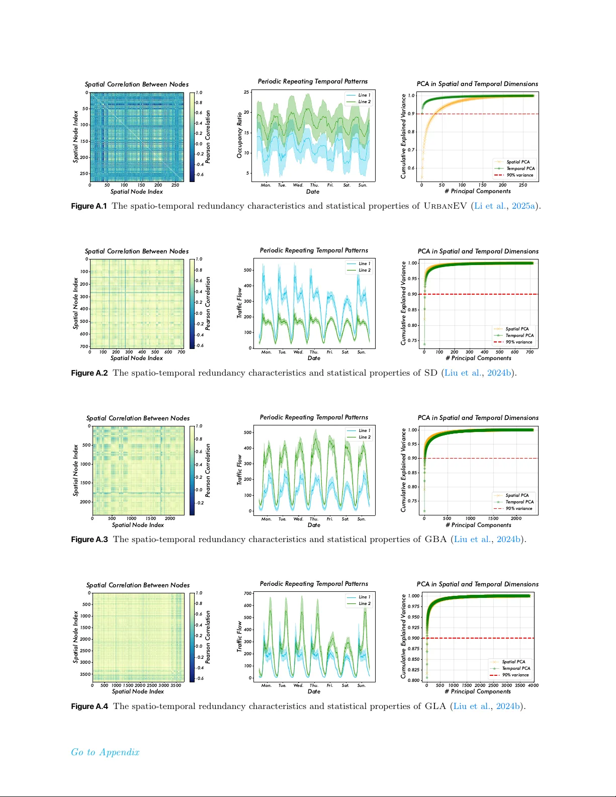
Learning from Complexity: Exploring Dynamic Sample Pruning of Spatio-Temporal Training Wei Chen 1,2 , Junle Chen 1 , Yuqian Wu 2 , Yuxuan Liang 2 ∗ , Xiaofang Zhou 1 ∗ 1 HKUST, 2 HKUST(GZ) Spatio-temporal forecasting is fundamental to intelligent systems in transportation, climate science, and urban planning. However, training deep learning models on the massive, often redundant, datasets from these domains presents a significant computational bottleneck. Existing solutions typically focus on optimizing model architectures or optimizers, while overlooking the inherent inefficiency of the training data itself. This conventional approach of iterating over the entire static dataset each epoch wastes considerable resources on easy-to-learn or repetitive samples. In this paper, we explore a novel training-efficiency techniques, namely learning from complexity with dynamic sample pruning, ST-Prune , for spatio-temporal forecasting . Through dynamic sample pruning, we aim to intelligently identify the most informative samples based on the model’s real-time learning state, thereby accelerating convergence and improving training efficiency. Extensive experiments conducted on real-world spatio-temporal datasets show that ST-Prune significantly accelerates the training speed while maintaining or even improving the model performance, and it also has scalability and universality. Correspondence: onedeanxxx@gmail.com, yuxliang@outlo ok.com, zxf@cse.ust.hk Date: Jan 28, 2026 1 Introduction With the rapid adv ancemen t of sensing tec hnologies, massive v olumes of spatio-temp oral data are b eing collected and lev eraged in data-driv en forecasting scenarios, enabling critical services ranging from traffic managemen t to weather forecasting and p ow er grid op erations ( A vila and Mezić , 2020 ; Nguyen et al. , 2023 ). T o capture the complex nonlinear dynamics inheren t in suc h data, spatio-temp oral neural netw orks ( Jin et al. , 2023 , 2024 ) hav e b ecome the dominant and most pow erful paradigm. How ever, while researc h communit y has largely fo cused on designing increasingly sophisticated architectures for marginal p erformance gains ( Shao et al. , 2024 ), a fundamental and c ostly b ottlene ck has b e en overlo oke d: the tr aining pr o c ess itself. Standard spatio-temp oral training protocols require iterating o ver the en tire samples in every training ep och ( Liu et al. , 2024b ). As a result, the widely adopted b enchmarks ( Li et al. , 2018 ; Song et al. , 2020 ) are typically restricted to limited spatial regions and temporal spans, severely limiting the scalabilit y of spatio-temp oral n ueral netw orks training and inflating their computational cost. This raises a natural research question: do we r e al ly ne e d to c ompute over al l available sp atio-temp or al samples during tr aining stage? T o answ er this question, w e first conduct a detailed analysis of the widely used spatio-temporal benchmark ( PeMS08 ). As shown in Figure 1 , the left panel visualizes the Pearson correlation matrix across spatial no des, rev ealing that the v ast ma jority exhibit high similarit y ( ≥ 0 . 8 ). Even no de pairs with lo w er similarit y still displa y recurring p erio dic temporal patterns, as illustrated in the middle panel. Principal comp onen t analysis (PCA) along both spatial and temp oral dimensions (right panel) further sho ws that a small n umber of components are sufficien t to reconstruct most of the v ariance. T o gether, these statistics r eve al a high de gr e e of sp atio-temp or al r e dundancy, which op ens up new opp ortunities for mor e efficient utilization of tr aining data. Recen t data-cen tric acceleration researc h ( Zha et al. , 2025 ) ha ve devoted significant effort to iden tifying unbiased or represen tative subsets within training datasets. T ypical tec hniques include data pruning ( Ra ju et al. , 2021 ; W ang et al. , 2023 ; Qin et al. , 2024 ; Zhang et al. , 2024b , a ; W ang et al. , 2025 ), dataset distillation ( Nguy en et al. , 1 0 20 40 60 80 100 120 140 160 Spatial Node Index 0 20 40 60 80 100 120 140 160 Spatial Node Index Spatial Correlation Between Nodes 0.2 0.4 0.6 0.8 1.0 P earson Correlation Mon. T ue. W ed. Thu. F ri. Sat. Sun. Date 0 100 200 300 400 500 600 700 800 T raffic Flow P eriodic R epeating T emporal P atterns Line 1 Line 2 0 25 50 75 100 125 150 175 # P rincipal Components 0.825 0.850 0.875 0.900 0.925 0.950 0.975 1.000 Cumulative Explained V ariance PCA in Spatial and T emporal Dimensions Spatial PCA T emporal PCA 90% variance Figure 1 The spatio-temp oral data redundancy c haracteristics and statistical properties along the spatial and temp oral dimensions, exemplified b y the PeMS08 ( Song et al. , 2020 ) dataset. F or more statistical information on other datasets, please refer to App endix A.1 . Spatial Averag e Temporal Average Avg: 2899.05 Std: 438.08 Avg: 204.63 Std: 114.17 Average Spatial Averag e Temporal Average Avg: 2918.55 Std: 559.39 Avg: 206.01 Std: 145.75 Average Global Hardn ess: 1 7 .05 Global Hardn ess: 1 7 . 1 6 ≈ Spatial Complexity Temporal Complexity (a) Illustration of the Averaging Masking Eff ect. ST Error Map of Sample B ST Error Map of Sample A ≠ ≠ (b) Distribution of Dynamic Intensit y & P atterns of Select ed Samples Figure 2 F urther analysis of spatio-temp oral data insights. (a) A veraging Masking Effect: Lo w-error no des dilute critical lo calized anomalies, necessitating a structural scoring mec hanism b ey ond simple mean error. (b) Long-tail S tationarit y Distribution: The dominance of stationary patterns motiv ates our stationarity-a w are rescaling to preven t distribution shift and maintain representativ eness. 2021 ; W ang et al. , 2022 ; Cazenav ette et al. , 2022 ; Zhao and Bilen , 2023 ; Li et al. , 2023 ; Zhang et al. , 2024c ), and coreset selection ( Har-Peled and Mazumdar , 2004 ; Chen , 2009 ; T onev a et al. , 2018 ; Shim et al. , 2021 ), whic h resp ectiv ely retain, synthesize, or select a smaller yet information-ric h subset from the original data. Despite their promise , these metho ds are primarily developed for computer vision and natural language pro cessing tasks and fail to ful ly exploit the unique r e dundancy char acteristics of sp atio-temp or al data highlighte d ab ove. T o address this critical gap, we prop ose ST-Prune , a nov el dynamic sample pruning framework sp ecifically tailored for spatio-temp oral training. Distinct from traditional paradigms that passively pro cess the entire dataset, ST-Prune activ ely curates high-v alue data subsets to optimize training efficiency . Our fundamental insigh t is that directly applying generic dynamic pruning strategies ( Ra ju et al. , 2021 ; Qin et al. , 2024 ; Moser et al. , 2025 ) to spatio-temp oral data pro v es ineffective. This failure stems from tw o sp ecific phenomena: the Aver aging Masking Effe ct (Figure 2 a) , where critical lo calized failures are obscured by low global errors, and the inherent L ong-tail Stationarity Distribution (Figure 2 b), where standard pruning induces sev ere distribution shifts. T o this end, ST-Prune op erationalizes these insigh ts via tw o inno v ative comp onen ts: complexit y-informed scoring metric, whic h incorp orates a spatio-temp oral heterogeneity p enalty to identify structural samples that app ear ”globally trivial yet locally intractable“; and stationarity-a ware gradien t rescaling, which adaptively adjusts w eights based on dynamic in tensity . This ensures that the preserved samples maintain an unbiased representation of the original data distribution while discarding substantial redundan t stationary samples. Ultimately , this design not only significantly mitigates computational o v erhead but also ensures the robust capture of div erse and complex spatio-temp oral patterns. In summary , our con tributions are: • W e propose ST-Prune , a dynamic sample pruning method of spatio-temporal training, that shifts the spatio-temp oral research fo cus from solely optimizing the mo del to intelligen tly optimizing the data flow 2 during training. • W e design a no v el framew ork consisting of a complexit y-informed difficulty metric to assess sample informativ eness in real-time and an stationarity-a ware distribution rescaling to ensure stable and effective training. • Extensiv e exp eriments on m ultiple real-w orld spatio-temooral datasets demonstrate that ST-Prune drastically reduces training time while maintaining or even improving the predictive accuracy of v arious backbones, pro ving its effectiveness, efficiency , and universalit y . 2 Related Work Efficien t Spatio-T emp oral T raining. Spatio-temp oral forecasting tasks t ypically rely on neural netw orks that integrate spatial and temp oral op erators ( Chen and Liang , 2025a , b ) to capture spatial dep endencies and temp oral dynamics. How ever, the large num b er of no des and extended time horizons ( Liu et al. , 2024b ; Yin et al. , 2025 ) result in substantial computational costs during training. Previous studies hav e sought efficiency impro vemen ts through mo del-level optimizations, such as prior structure Shao et al. ( 2022 ); Cini et al. ( 2023 ); F u et al. ( 2025 ), graph sparsification ( W u et al. , 2025 ; Ma et al. , 2025 ), and mo del distillation ( T ang et al. , 2024 ; Chen et al. , 2025 ), or sample-level transformations, including subgraph ( Jiang et al. , 2023 ; Liu et al. , 2024a ; W ang et al. , 2024 ; W eng et al. , 2025 ; Zhao et al. , 2026 ) and input window ( F ang et al. , 2025 ; Oc k erman et al. , 2025 ; Shao et al. , 2025 ) sampling. While these approaches reduce computational demand at the mo del or optimization level, they rarely provide explicit con trol ov er the num b er or distribution of training samples and often tightly couple netw ork comp onent design. In c ontr ast, we aim to develop a gener al dynamic sp atio-temp or al sample pruning str ate gy that ac c eler ates the tr aining of arbitr ary sp atio-temp or al neur al networks while maintaining c omp etitive p erformanc e. Data-Cen tric Acceleration Strategy . Data-cen tric acceleration strategies ( Zha et al. , 2025 ) hav e drawn considerable attention b ecause they enhance mo del training and inference efficiency from a data manageme n t p erspective. Represen tativ e approaches include data distillation ( Lei and T ao , 2023 ; Y u et al. , 2023 ), data pruning, and data selection ( Moser et al. , 2025 ). Data distillation seeks to compress the original data distribution into a smaller yet information-equiv alent synthetic dataset to reduce training cost, whereas data pruning and selection reduce computational burden by removing redundant samples or selecting the most represen tativ e subsets. Ho w ev er, these metho ds are primarily designed for vision ( W ang et al. , 2018 ) or language ( Albalak et al. , 2024 ) tasks and struggle to exploit the high redundancy and strong correlations inheren t in spatio-temp oral data. Moreo ver, they are often static and sensitive to sample size ( Guo et al. , 2022 ), which may limit generalization under dynamically evolving spatio-temp oral distributions. Notably, our method exploits the c omplexity of ST samples and dynamic al ly adjusts sample sele ction to maximize c omputational efficiency. 3 Preliminaries Prob elm Definition (Spatio-T emp oral F orecasting). F rom an optimization p ersp ective, spatio-temp oral forecasting aims to solve an empirical risk minimization problem. Given a large-scale spatio-temp oral training dataset D = { ( X i , Y i ) } |D| i =1 (and an optional graph structure prior G ), the ob jectiv e is to find the optimal mo del parameters θ ∗ b y minimizing a global loss function J ( θ ; D ) : min θ J ( θ ; D ) = 1 |D | |D| X i =1 L ( f θ ( X i ; G ) , Y i ) , (1) where f θ is the forecasting spatio-temp oral neural netw ork, and L is a loss metric ( e . g ., MAE). ( X i ∈ R N × T p × F , Y i ∈ R N × T f × F ) represent the sensor readings of C measuremen t features at N spatial lo cations o v er T p past and T f future consecutive time steps, resp ectiv ely . This formulation treats every sample ( X i , Y i ) equally and implies that the gradien t for each training ep o c h is computed o ver the entire, often redundan t, dataset D . This exhaustive summation is the primary source of computational inefficiency in the spatio-temp oral training pro cess. 3 T ask Definition (Dynamic Sample Pruning). W e formulate dynamic sample pruning as an optimization problem aimed at approximate the conv ergence of the ob jective in Equation 1 . Instead of using the full dataset D at each ep o ch e , we seek to ide n tify an optimal training subset D ∗ e ⊂ D with a constrained size |D e | = k e < |D | . The mo del parameters are then up dated based only on this subset: θ e = Up date ( θ e − 1 , D e ) . Ideally , the optimal subset D ∗ e should b e the one that provides the steep est descent direction for the true, underlying data distribution P : D ∗ e = argmin D e ⊂D , |D e | = k e E ( X,Y ) ∼P [ L ( f θ e ( X ; G ) , Y )] . (2) Ho w ev er, minimizing this ob jective is in tractable as the true distribution P is unkno wn. How ever, we ha v e empirically s ho wn ab ov e that this distribution exhibits a significant low-rank prop ert y , that is, the training samples are highly redundant. Th us, the core challenge of dynamic sample pruning is to design a tractable and efficient proxy strategy to select an informative subset D e at each ep o c h. 4 Methodology Initialize : Mo del 𝜃 , Score Memory ℋ , W eights 𝑊 Prune Easy Samples Update Weights for Unbiasedness Set Active Batch 𝐼 ! Full - Sample Supervised Annealing Forward & Compute Loss Update Score Memory Compute Weighted Objective No Phase 1: Complexity- Informed Prunin g Phase 2: Stability - Guided O ptimization Backward & Update 𝜃 Easy Samples Easy Samples Hard Samples C Unbiased Expectation Rescaling Ensures unbiased gradient expectation: 𝐸 ∇𝑗 ≈ ∇ ' 𝚥 Sampled & Rescaled (Af ter) After Pruning Ye s Hard Samples Before Prun ing Random Sampl ing (p) (a) Overview of ST - Prune workflo w Reweighting ( ×𝑤 ! ) Epoc h ≤ 𝛿 ⋅ 𝐸 (b) Complexity - Informed Pruning Figure 3 The ov erall workflo w of the ST-Prune for efficient data pruning during spatio-temp oral training. 4.1 Complexity-Informed Pruning 4.1.1 Beyond The Averaging Masking Effect Before elab orating on our prop osed framew ork, we first analyze the limitations of standard dynamic pruning tec hniques ( Katharop oulos and Fleu ret , 2018 ; Ra ju et al. , 2021 ; Qin et al. , 2024 ) when applied to spatio- temp oral domains. Existing metho ds t ypically quantify sample difficult y using a global loss metric, ℓ i = ∥ f θ ( X i ) − Y i ∥ , where a low er ℓ i indicates an “easy” sample. How ever, in spatio-temp oral forecasting, the scalar loss ℓ i is an aggregate metric av eraged ov er N spatial no des and T time steps. This aggregation introduces a critical pathology w e term the Aver aging Masking Effe ct .W e empirically demonstrate this phenomenon in Figure 2 (a), which visualizes the error landscap es of tw o distinct samples from a real-world traffic dataset: • Sample A (Global Noise): The error is distributed relatively uniformly across the spatio-temp oral field. The global hardness (mean MAE) is calculated as 17.05. • Sample B (Lo cal Anomaly): As highlighted by the red circle in Figure 2 (a), this sample contains critical lo calized failures ( e . g ., severe congestion spikes at sp ecific hubs), while the remaining no des exhibit lo w errors. Surprisingly , its global hardness is 17.16. Despite the fundamental diffe rence in structural information, standard pruning metho ds viewing only the global hardness ( ≈ 17 . 1 ) would treat these tw o samples as identical. Consequen tly , the informative Sample B, whic h drives the learning of lo cal spatial dynamics, ma y risks b eing pruned as “easy” data. This observ ation confirms that magnitude-based metrics fail to distinguish structural complexity from background noise. T o address this, we prop ose Sp atio-T emp or al Complexity Sc oring , a metric designed to capture the non-uniformity ( σ ) of the error distribution, ensuring that samples with high spatial heterogeneity (like Sample B) are preserv ed even if their global mean is low. 4 4.1.2 Spatio-Temporal Complexity Scoring F ormally , we prop ose ST-Prune . As shown in Fig. 3 , during the forw ard propagation pro cess, each sample retains a score related to its loss v alue. The av erage of these scores is set as the pruning threshold. In eac h ep och, a corresp onding prop ortion of samples with low scores are pruned. T o op erationalize the insigh t from Figure 2 (a), we prop ose a comp osite scoring function that explicitly p enalizes p erformance heterogeneit y . Let E ( i ) t ∈ R N × T denote the absolute error matrix for the i -th sample at ep och t . W e define the structural informativeness score H t ( i ) as: H t ( i ) = µ ( E ( i ) t ) | {z } Global Hardness + λ ·    σ space ( E ( i ) t ) + σ time ( E ( i ) t ) | {z } Spatio-T emp oral Complexity    , (3) where µ ( · ) denotes the global mean. The terms σ space and σ time represen t the standard deviations calculated along the spatial and temp oral dimensions, resp ectively . 4.1.3 Randomized Pruning Policy T o reduce computational ov erhead while maintaining data diversit y , we categorize samples into an Informative Set S inf and a R e dundant Set S red at the b eginning of eac h ep o ch t . Let ¯ H t b e the av erage score of the en tire dataset. z i ∈ ( S inf , if H t ( i ) ≥ ¯ H t S red , if H t ( i ) < ¯ H t (4) Unlik e static pruning which p ermanen tly discards S red , w e adopt a randomized “soft” pruning strategy . All samples in S inf are retained. F or samples in S red , we retain them with a probability p ∈ (0 , 1) , determined b y the target pruning ratio. This ensures that even currently ”easy“ samples hav e a chance to b e revisited, prev en ting the mo del from catastrophic forgetting of basic patterns. 4.2 Stability-Guided Optimization 4.2.1 Stationarity-Aware Gradient Rescaling While the scoring metric iden tifies which samples to prune, a naiv e remov al of “easy” samples would inevitably alter the training data distribution. As highligh ted in Figure 2 (b), spatio-temp oral datasets exhibit a long-tail distribution of dynamic intensit y: the v ast ma jorit y of samples are stationary (lo w temp oral v ariance), while high-dynamic even ts are rare. Standard pruning techniques Qin et al. ( 2024 ), whic h apply a uniform rescaling w eigh t w = 1 1 − r (where r is the pruning rate), fail to account for this imbalance. By disprop ortionately remo ving stationary samples, they shift the training distribution tow ards the “tail" (non-stationary even ts), causing the mo del to ov erfit to extreme dynamics and lose robustness on regular patterns. T o rectify this distribution shift, we prop ose a Stationarity-Awar e R esc aling strategy . W e first quantify the dynamic intensity δ i of each sample i as the temp oral v ariance of its ground truth targets: δ i = V ar t ( Y i ) . F or the subset of retained “inf" samples S ′ inf , we assign an adaptive weigh t w i that is inv ersely prop ortional to their dynamic intensit y: w i = 1 1 − r ·  ¯ δ D δ i + ϵ  α | {z } Stationarity Correction , (5) where ¯ δ D is the global av erage intensit y , and α ≥ 0 controls the correction strength. This mechanism ensures that preserv ed stationary samples ( lo w δ i ) receiv e higher weigh ts, effectiv ely representing the p opulation of pruned stationary data. Conv ersely , highly dynamic samples ( high δ i ) hav e b een naturally retained through our scoring metric and will receive standard weigh ts. F ormally , the mo dified ob jectiv e ˜ J ( θ ) for the current ep och b ecomes: ˜ J ( θ ) = X i ∈S red L ( x i , y i ; θ ) + X j ∈S ′ inf w j · L ( x j , y j ; θ ) . (6) 5 This reweigh ting guarantees that the gradient exp ectation remains unbiased not only in magnitude but also in terms of dynamic r e gime distribution , ensuring conv ergence consistency with the full dataset. 4.2.2 Training Schedule with Annealing While the unbiased estimator holds in exp ectation, the v ariance of the gradients inevitably increases due to do wnsampling. T o mitigate this effect and ensure stable conv ergence in the final phase of training, we in tro duce a deterministic annealing strategy . Given a total training budget of E ep ochs and a cutoff ratio δ ( e . g ., δ = 0 . 9 ), we p erform the pruning strategy only for the first δ · E ep ochs. F or the remaining ep o chs t > δ · E , w e rev ert to full-dataset training. This allows the mo del to fine-tune on all samples, eliminating an y residual v ariance and ensuring that the final mo del p erformance is strictly lossless compared to the baseline. 5 Experiments In this section,we conduct extensive exp eriments to answer the following research questions (RQs): • R Q1: Can ST-Prune outp erform existing data pruning metho ds in v arious ST datasets? ( Effe ctiveness ) • RQ2: Ho w do es the efficiency of ST-Prune compare with that of the existing baseli nes? ( Efficiency ) • R Q3: How scalable is ST-Prune with resp ect to large-scale datasets and foundation mo dels? ( Sc alability ) • RQ4: Is ST-Prune effective across different types of backbones, optimizers, and tasks? ( Universality ) • R Q5: How do es ST-Prune w ork? Whic h comp onents pla y the k ey roles, and are they sensitive to parameter settings or comp onen t designs? ( Me chanism & R obustness ) 5.1 Experimental Setup Dataset and Ev aluation Proto col. W e ev aluate our metho d on representativ e ST b enchmarks: PEMS08 ( Song et al. , 2020 ) from the traffic domain and Urb anEV ( Li et al. , 2025a ) from the energy domain, alongside the large-scale b enchmark L ar geST ( Liu et al. , 2024b ) for scalability analysis. F ollowing standard proto cols ( Shao et al. , 2024 ; Jin et al. , 2023 ), datasets are split chronologically (6:2:2) to forecast the next 12 steps giv en the past 12. T o ensure rigorous efficiency comparison, we disable early stopping and train for a fixed 100 ep ochs. Each exp erimen t was rep eated five times and the mean was rep orted. Performance under different pruning levels is assessed via MAE, RMSE, and MAPE across data retention ratios of {10%, 30%, 50%, 70%}. F urther details of datasets and proto cols in App endix A.1 . Baselines and Parameter Settings. W e b enc hmark against a comprehensive suite of pruning strategies adapted for spatio-temp oral tasks, categorized into: (1) Static metho ds : Random ( Har d R andom ), geometry- based ( CD , Her ding , K-Me ans ), uncertaint y-based ( L e ast Confidenc e , Entr opy , Mar gin ), loss-based ( F or getting , Gr aNd ), decision boundary-based ( Cal ), bi-lev el ( Glister ), and submo dular ( Gr aphCut , F aL o ); and (2) Dynamic metho ds : Random( Soft R andom ), uncertaint y-based ( ϵ -gr e e dy , UCB ), and loss-based ( InfoBatch ). W e employ GWNet ( W u et al. , 2019 ) as the default backbone, alongside ST AEformer ( Liu et al. , 2023 ) and STID ( Shao et al. , 2022 ) for cross-architecture ev aluation, and the foundation mo del Op enCity ( Li et al. , 2025b ) to assess scalability . T o ensure fair comparison, all mo dels are trained using SGD (momentum 0.9, w eigh t decay 1e-4) with a cosine annealing scheduler. More details on baselines, mo dels, and parameters are pro vided in App endix A.2 . 5.2 Effectiveness Study (RQ1) T able 1 compares the MAPE results of ST-Prune against representativ e data pruning and selection metho ds. The b est results are highligh ted in b old pink , and the second-b est in underlined in blue . Besides, we rep ort the relative p erformance change ( ↓ deg radation or ↑ improv ement ) compared to the whole dataset baseline. W e observ e that: ❶ Dynamic pruning str ate gies gener al ly outp erform static ones. A cross v arious baselines, dynamic metho ds achiev e sup erior p erformance by lev eraging training dynamics to better assess sample imp ortance. In terestingly , b oth Hard Random and Soft Random remain comp etitive at low retention rates, mirroring phenomena observed in vision datasets ( Guo et al. , 2022 ). W e hypothesize that for strategy-based 6 Table 1 P erformance comparison to state-of-the-art dataset selection and pruning metho ds when remaining { 10% , 30% , 50% , 70% } of the full training set. All methods are trained using same ST backbone. (Additional MAE and RMSE results are provided in App endix B ) Dataset Pems08 ( MAPE (%) ↓ ) UrbanEV ( MAPE (%) ↓ ) Remaining Ratio % 10 30 50 70 10 30 50 70 Static Hard Random 13.93 ↓ 26 . 87% 14.80 ↓ 34 . 79% 12.07 ↓ 9 . 93% 12.06 ↓ 9 . 84% 35.89 ↓ 20 . 32% 31.90 ↓ 6 . 94% 31.52 ↓ 5 . 67% 30.69 ↓ 2 . 88% CD ( Agarwal et al. , 2020 ) 14.55 ↓ 32 . 51% 12.25 ↓ 11 . 57% 11.96 ↓ 8 . 93% 11.83 ↓ 7 . 74% 38.37 ↓ 28 . 63% 32.20 ↓ 7 . 95% 30.40 ↓ 1 . 91% 31.01 ↓ 3 . 96% Herding ( W elling , 2009 ) 15.79 ↓ 43 . 81% 12.11 ↓ 10 . 29% 11.58 ↓ 5 . 46% 12.84 ↓ 16 . 94% 34.63 ↓ 16 . 09% 30.97 ↓ 3 . 82% 30.94 ↓ 3 . 72% 30.97 ↓ 3 . 82% K-Means ( Sener and Sav arese , 2018 ) 15.71 ↓ 43 . 08% 12.24 ↓ 11 . 48% 12.48 ↓ 13 . 66% 11.52 ↓ 4 . 92% 38.45 ↓ 28 . 90% 31.85 ↓ 6 . 77% 30.96 ↓ 3 . 79% 30.69 ↓ 2 . 88% Least Confidence ( Coleman et al. , 2019 ) 14.31 ↓ 30 . 33% 12.62 ↓ 14 . 94% 11.74 ↓ 6 . 92% 11.61 ↓ 5 . 74% 34.23 ↓ 14 . 75% 36.87 ↓ 23 . 60% 30.98 ↓ 3 . 86% 30.55 ↓ 2 . 41% Entrop y ( Coleman et al. , 2019 ) 13.22 ↓ 20 . 40% 12.82 ↓ 16 . 76% 12.83 ↓ 16 . 85% 11.28 ↓ 2 . 73% 36.42 ↓ 22 . 09% 31.20 ↓ 4 . 59% 30.65 ↓ 2 . 75% 30.49 ↓ 2 . 21% Margin ( Coleman et al. , 2019 ) 14.06 ↓ 28 . 05% 12.55 ↓ 14 . 30% 11.60 ↓ 5 . 65% 11.38 ↓ 3 . 64% 37.21 ↓ 24 . 74% 31.89 ↓ 6 . 91% 32.73 ↓ 9 . 72% 30.89 ↓ 3 . 55% F orgetting ( T oneva et al. , 2018 ) 14.92 ↓ 35 . 88% 12.19 ↓ 11 . 02% 11.46 ↓ 4 . 37% 11.29 ↓ 2 . 82% 32.84 ↓ 10 . 09% 31.36 ↓ 5 . 13% 30.63 ↓ 2 . 68% 30.69 ↓ 2 . 88% GraNd ( Paul et al. , 2021 ) 13.93 ↓ 26 . 87% 13.09 ↓ 19 . 22% 12.33 ↓ 12 . 30% 11.50 ↓ 4 . 74% 35.26 ↓ 18 . 20% 31.71 ↓ 6 . 30% 30.90 ↓ 3 . 59% 30.20 ↓ 1 . 24% Cal ( Margatina et al. , 2021 ) 14.79 ↓ 34 . 70% 12.40 ↓ 12 . 93% 12.64 ↓ 15 . 12% 12.40 ↓ 12 . 93% 33.77 ↓ 13 . 21% 32.25 ↓ 8 . 11% 31.45 ↓ 5 . 43% 30.81 ↓ 3 . 29% Glister ( Killamsetty et al. , 2021 ) 14.48 ↓ 31 . 88% 13.23 ↓ 20 . 49% 12.51 ↓ 13 . 93% 11.74 ↓ 6 . 92% 33.70 ↓ 12 . 97% 33.65 ↓ 12 . 81% 32.78 ↓ 9 . 89% 31.26 ↓ 4 . 79% GraphCut ( Iyer et al. , 2021 ) 15.07 ↓ 37 . 25% 12.26 ↓ 11 . 66% 11.84 ↓ 7 . 83% 11.27 ↓ 2 . 64% 35.73 ↓ 19 . 78% 31.49 ↓ 5 . 56% 30.76 ↓ 3 . 12% 31.23 ↓ 4 . 69% F aLo ( Iyer et al. , 2021 ) 15.95 ↓ 45 . 26% 12.56 ↓ 14 . 39% 12.13 ↓ 10 . 47% 11.40 ↓ 3 . 83% 35.07 ↓ 17 . 57% 31.72 ↓ 6 . 34% 31.23 ↓ 4 . 69% 31.01 ↓ 3 . 96% Dynamic Soft Random 15.00 ↓ 36 . 61% 12.41 ↓ 13 . 02% 12.01 ↓ 9 . 38% 11.34 ↓ 3 . 28% 33.55 ↓ 12 . 47% 31.34 ↓ 5 . 06% 30.48 ↓ 2 . 18% 30.35 ↓ 1 . 74% ϵ -greedy ( Ra ju et al. , 2021 ) 13.82 ↓ 25 . 87% 12.21 ↓ 11 . 20% 11.84 ↓ 7 . 83% 11.24 ↓ 2 . 37% 33.25 ↓ 11 . 46% 30.98 ↓ 3 . 86% 30.46 ↓ 2 . 11% 30.30 ↓ 1 . 58% UCB ( Ra ju et al. , 2021 ) 13.80 ↓ 25 . 68% 12.41 ↓ 13 . 02% 11.76 ↓ 7 . 10% 11.28 ↓ 2 . 73% 33.24 ↓ 11 . 43% 31.08 ↓ 4 . 19% 30.43 ↓ 2 . 01% 30.29 ↓ 1 . 54% InfoBatch ( Qin et al. , 2024 ) 13.66 ↓ 24 . 41% 12.12 ↓ 10 . 38% 11.83 ↓ 7 . 74% 11.33 ↓ 3 . 19% 32.02 ↓ 7 . 34% 30.78 ↓ 3 . 18% 30.24 ↓ 1 . 37% 29.83 ↓ 0 . 00% ST-Prune ( Our ) 12.13 ↓ 13.21 11.75 ↓ 7.01 11.11 ↓ 5.56 11.19 ↓ 2.82 29.56 ↑ 0.91 29.42 ↑ 1.37 29.15 ↑ 2.28 29.05 ↑ 2.61 Whole Dataset 10.98 ± 0 . 23 29.83 ± 0 . 09 100% 90% 70% 50% 30% 10% P er Epoch Time (UrbanEV) 3.6 3.8 4.0 4.2 4.4 4.6 4.8 MAE V anilla H-R andom Margin Herding F orgetting S -R andom Cal InfoBatch Glister ST -P rune 100% 90% 70% 50% 30% 10% P er Epoch Time (UrbanEV) 6.5 7.0 7.5 8.0 8.5 9.0 RMSE V anilla H-R andom Margin Herding F orgetting S -R andom Cal InfoBatch Glister ST -P rune 100% 90% 70% 50% 30% 10% P er Epoch Time (UrbanEV) 28 30 32 34 36 38 40 MAPE(%) V anilla H-R andom Margin Herding F orgetting S -R andom Cal InfoBatch Glister ST -P rune Figure 4 The trade-off betw een per-ep o ch time and p erformance in Urb anEV . Specifically , we report the test p erformance when metho ds achiev e p er ep o ch times of {10%, 30%, 50%, 70%, 90%} of the full dataset training time. “V anilla” denotes the full dataset training result. metho ds, sp ecific algorithmic inductive biases ma y introduce a harmful sampling exp ectation bias. ❷ Dataset r e dundancy varies acr oss domains. W e observ e that PEMS08 is more sensitive to pruning than Urb anEV , indicating differing redundancy levels. F or example, at 10% retention (excluding our metho d), p erformance degradation on PEMS08 ( 20 . 40% ∼ 45 . 26% ) significan tly exceeds that of Urb anEV ( 7 . 34% ∼ 28 . 63% ). Ho w ev er, p erformance recov ers rapidl y as the retention ratio increases; at a 50% pruning level, degradation across b oth datasets remains within single digits. ❸ ST-Prune c onsistently exc els acr oss al l pruning r atios. ST-Prune outp erforms b oth static and dynamic baselines in all settings. Ev en at 10% retention rate, it k eeps practical utility with minimal degradation. Notably , ST-Prune surpasses whole dataset p erformance on Urb anEV . W e attribute this to Urb anEV ’s low redundancy and high signal-to-noise ratio, where our metho d effectiv ely filters noise to b o ost p erformance. 5.3 Efficiency Study (RQ2) Figure 4 illustrates the efficiency comparison. W e observe the following: ❹ ST-Prune strikes a sup erior b alanc e b etwe en tr aining time and p erformanc e, significantly outperforming other baselines. Notably , ST-Prune ac hiev es nearly 2 × acceleration ( ≈ 50% reduction in p er-ep o ch time) with negligible p erformance loss across different 7 metrics. ❹ Ev en under an aggressive 10 × sp eedup, ST-Prune incurs only marginal degradation, maintaining acceptable p erformance where comp eting metho ds deteriorate rapidly . 5.4 Scalability Study (RQ3) T o assess the scalability of our method, w e conduct ev aluations from b oth data and mo del p ersp ectives. Sp ecifically , we v alidate p erformance using the representativ e large-scale spatio-temp oral dataset L ar geST ( Liu et al. , 2024b ), which comprises the SD, GBA, and GLA subsets. A dditionally , we employ the spatio-temp oral foundation mo del Op enCity ( Li et al. , 2025b ) across the Mini, Base, and Plus scales. Table 2 Comparison of ST-Prune with the fastest dynamic pruning metho d Soft R andom on L argeST . TIME: T otal w all-clo c k time. Dataset SD ( #716 ) GBA ( #2352 ) GLA ( #3834 ) MAE RMSE MAPE (%) TIME MAE RMSE MAPE (%) TIME MAE RMSE MAPE (%) TIME Whole Dataset 24.13 ± 1 . 14 38.03 ± 1 . 32 15.77 ± 0 . 87 2.07h 27.34 ± 1 . 04 42.11 ± 1 . 19 24.11 ± 0 . 48 13.05h 26.26 ± 0 . 84 41.12 ± 1 . 47 16.06 ± 0 . 63 30.53h Soft R andom (10%) 30.41 47.96 20.43 0.52h 33.05 48.71 39.30 2.97h 29.74 45.98 20.97 7.25h ST-Prune (10%) 24.01 37.73 15.51 0.61h 27.32 41.94 24.05 4.92h 26.22 40.88 15.95 13.38h ST-Prune (1%) 24.76 38.19 16.51 0.31h 28.16 42.77 23.64 2.84h 26.95 41.57 17.62 7.12h Improv ement ↑ 21 . 05% ↑ 21 . 33% ↑ 24 . 08% × 6 . 68 ↑ 17 . 33% ↑ 13 . 90% ↑ 38 . 80% × 4 . 60 ↑ 11 . 84% ↑ 11 . 09% ↑ 23 . 94% × 4 . 29 Large-Scale Datasets. T able 2 presents comparative p erformance on the LargeST b enchmark. W e highlight the following observ ations: ❶ Comp etitive efficiency-p erformanc e tr ade-off. At a 10% data retention rate, heuristic baselines ( i . e ., Soft R andom ) ac hieve the fastest dynamic pruning speeds but suffer significan t p erformance degradation. In contrast, our metho d achiev es relative p erformance gains of 11 . 09% ∼ 38 . 80% o v er heuristics and even slightly outp erforms full-data training, despite the additional computational ov erhead incurred by our customized p olicy design. ❷ R obustness acr oss sp atio-temp or al sc ales. Unlik e heuristic baselines ( i . e ., Soft R andom ) that exhibit marked p erformance drops on smaller datasets ( e . g ., SD), our ST-Prune main tains consistent p erformance adv antages across v arying spatio-temp oral scales. ❸ Sup erior efficiency and sc alability. Even in extreme 1% retention scenarios, our mo del retains comp etitiv e p erformance while drastically reducing computational costs. By cutting training time from days to hours, it demonstrates significan t p oten tial for data scalability and large-scale deploymen t. Figure 5 Performance and efficiency trade-offs b etw een w/o and w/ ST-Prune at different scales of the ST-foundation mo del OpenCity . ST-F oundation Mo dels. F ollowing ( Li et al. , 2025b ) settings, w e further v alidate mo del scalability by in tegrating ST-Prune with the Op enCity foundation mo del series. Figure 5 illustrates the trade-off b et w een p er-epo ch pre-training time and downstream p erformance, revealing the following: ❶ Simultane ous gains in efficiency and c ap ability. ST-Prune ac hiev es a “win-win” outcome , with green arrow consistently p ointing to w ards the “most sample-efficient” region. Across all mo del scales, ST-Prune not only significantly reduces the pre-training time (shifting left) but also generally improv es the prediction accuracy (shifting upw ards). This suggests that our approach effectively purifies the pre-training corpus by eliminating noisy or redundant samples that hinder con v ergence. ❷ Demo cr atizing lar ge-sc ale mo del tr aining. F or the computation-intensiv e Plus scale, ST-Prune significan tly curtails p er-ep o c h training time ( e . g ., from ∼ 350 to 250 mins) while 8 outp erforming the original baseline. Notably , ST-Prune reduces the training cost of the Base scale to a level smaller than the Mini scale, thus effectively training larger and more p ow erful mo dels under constrained computational resources. 5.5 Universality Study (RQ4) Whole - GWNet (29.83%) Whole - STID (26.45%) Whole - ST AEformer (24.92%) 10% 30% 50% 70% R emaining R atio 25 26 27 28 29 30 MAPE (%) Cross -Architecture GWNet STID ST AEformer Whole - SGD (29.83%) Whole - A dam (23.63%) Whole - Muon (23.44%) 10% 30% 50% 70% R emaining R atio 23 24 25 26 27 28 29 30 MAPE (%) Cross - Optimizer SGD A dam Muon Whole - Short (29.83%) Whole - Medium (25.84%) Whole - L ong (37.19%) 10% 30% 50% 70% R emaining R atio 26 28 30 32 34 36 38 MAPE (%) Cross - T ask Short Medium L ong Figure 6 Performance v ariations across distinct architectures, optimizers, and tasks under data retention rates of { 10% , 30% , 50% , 70% } . T o ev aluate the universalit y of our metho d, we conduct ev aluations on Urb anEV across different bac kb ones, optimizers, and tasks. Sp ecifically , we v alidate p erformance using representativ e ST architectures including GWNet, STID, and ST AEformer; distinct optimizers such as SGD, A dam ( Kingma and Ba , 2015 ), and Muon ( Jordan et al. , 2024 ); and prediction horizons cov ering short-term ( i . e ., 12 → 12), medium-term ( i . e ., 24 → 24), and long-term ( i . e ., 96 → 96) tasks. F rom each subgraph in Figure 6 , we observed that: Cross-Arc hitecture Ev aluation. ❶ Universal p erformanc e gains. Notably , across all three backbones, mo d- els trained on ST-Prune -selected subsets (dashed lines) consistently outp erform their full-dataset counterparts (solid lines), achieving low er MAPE at most reten tion levels. ❷ Ar chite ctur al r obustness. In lo w-reten tion regimes, our metho d yields pronounced gains for light weigh t architectures like STID and GWNet. How ever, ev en for the adv anced, ov er-parameterized ST AEformer, our mo del can also push p erformance b oundaries as the retention ratio increases. Cross-Optimizer Ev aluation. ❶ R obust adaptability to optimization pr o c ess. ST-Prune main tains ef- fectiv eness regardless of the chosen optimizer. Notably , with SGD, ST-Prune ac hiev es substantial gains, outp erforming the full-dataset baseline even at low reten tion rates. ❷ Enhancing advanc e d optimizers. Ev en with state-of-the-art optimizers lik e Adam and the recent Muon, which already yield low error rates ( < 24% ), ST-Prune further pushes p erformance b oundaries. At retention rates ab ov e 30% , ST-Prune successfully filters detrimen tal noise, enabling b oth optimizers to surpass their full-dataset baselines, thereb y confirming the robustness of our metho d ST-Prune across diverse optimization landscap es. Cross-T ask Ev aluation. ❶ Short-to-me dium term r obustness. F or short and medium horizons, ST-Prune con- sisten tly outp erforms full-dataset baselines across all retention ratios, confirming that immediate temp oral dep endencies are effectively captured within compact, denoised subsets. ❷ L ong-term sensitivity. Although long-term inv olves more complex dep endencies and higher sensitivity to data scarcit y , our metho d remains robust; p erformance successfully recov ers to match full-dataset levels at a 50% retention ratio. 5.6 Mechanism & Robustness Study (RQ5) Ablation Study . T o v alidate the effectiv eness of eac h comp onen t in ST-Prune , w e compare against four v arian ts: removing the spatio-temp oral complexity score ( w/o STC ), the score rescaling strategy ( w/o R es. ), and the annealing scheduler ( w/o Anne. ). As sho wn in Figure 7 Left, ST-Prune consisten tly yields the low est errors across all retention ratios. W e observe that: ❶ Ne c essity of sche duling with anne aling. The p erformance degradation of w/o Anne. is the most significant, esp ecially under low retention rates, which illustrates its p ositiv e role in v ariance correction for sparse scenarios. ❷ Imp ortanc e of Sc oring Comp onents. Remo ving STC leads to noticeable error increases, indicating that b oth the intrinsic difficulty of samples and the historical consistency are critical for robust sample v aluation. 9 R emaining R atio: 10% 29.0 29.5 30.0 30.5 31.0 31.5 32.0 MAPE(%) 29.56 29.82 30.10 31.59 R emaining R atio: 30% 29.0 29.5 30.0 30.5 31.0 31.5 32.0 29.42 29.85 29.84 30.43 R emaining R atio: 50% 28.5 29.0 29.5 30.0 30.5 31.0 MAPE(%) 29.15 29.85 29.37 30.55 R emaining R atio: 70% 28.5 29.0 29.5 30.0 30.5 31.0 29.05 29.43 29.44 30.66 ST -P rune w/o ST C w/o R es. w/o Anne. 0.2 0.4 0.6 0.8 1.0 C o m p l e x i t y 29.0 29.2 29.4 29.6 MAPE (%) 10% 30% 50% 70% 0.80 0.85 0.90 0.95 1.00 A n n e a l i n g 29.0 29.5 30.0 30.5 31.0 31.5 MAPE (%) 10% 30% 50% 50% Figure 7 Ablation and parameter sensitivit y analysis on Urb anEV dataset under training data reten tion rates of { 10% , 30% , 50% , 70% } . P arameter Sensitivity . W e further inv estigate the sensitivit y of ST-Prune to k ey hyperparameters: the complexit y weigh t and the annealing rate . ❶ Imp act of Complexity W eight . Figure 7 (Middle) exhibits a con v e x trend for , where extreme v alues (to o small or to o large) hamp er p erformance. The optimal range lies b et ween 0.4 and 0.6, suggesting that balancing the raw loss with spatio-temp oral structural complexity is essen tial for identifying informative samples. ❷ Imp act of Anne aling R ate . Figure 7 (Righ t) reveals that p erformance is stable when δ ∈ [0 . 8 , 0 . 95] but deteriorates rapidly as δ approac hes 1 , i . e . w/o Anne. , consistent with previous observ ations in the ablation study . Whole Tr aining set Hard Random 20% 40% 60% 80% Info Batch 20% 40% 60% 80% Soft Random ST -Prune (Our) 20% 40% 60% 80% 20% 40% 60% 80% Figure 8 Visualization of t-SNE fixed-corner clustering of the PEMS08 distribution with the full training set and a reten tion rate of 20%. The right panel shows the evolution of selected subsets through different pruning strategies at differen t training progresses (20% to 80%). In terpretability Study . T o intuitiv ely understand how ST-Prune selects spatio-temp oral sample compared to baselines, we visualize the latent distribution of the selected subsets using t-SNE in Figure 8 . W e can observe that: ❶ Dynamic alignment with tr aining dynamics. While heuristic baselines ( e . g ., Har d/Soft R andom ) pro duce static, sparse distributions via uniform sampling, ST-Prune exhibits a clear evolutionary tra jectory , balancing the preserv ation of representativ e centroids with the exploration of global diversit y . ❷ R estor ation of intrinsic data top olo gy. Surpassing InfoBatch , ST-Prune rapidly reconstructs the approximate manifold top ology of the original distribution during training, thereby ensuring robust generalization p erformance. 6 Conclusion and Future Work In this pap er, w e in v estigate the redundancy inheren t in spatio-temp oral training datasets and explore effectiv e approaches for efficient dynamic data pruning. W e prop ose ST-Prune that uses complexity-informed scoring with stationarity-a ware gradien t rescaling to prioritize informative samples during training. Extensiv e exp erimen ts confirm its effectiveness. In future work, we aim to explore how to extend this metho d to con tinual spatio-temp oral forecasting where the spatial top ology evolv es ov er training time. 10 References Amit Agarwal, Bhumik a Gupta, Gaurav Bhatt, and Ankush Mittal. Construction of a semi-automated mo del for faq retriev al via short message service. In Pro ceedings of FIRE, 2015. Sharat Agarwal, Himansh u Arora, Saket Anand, and Chetan Arora. Contextual div ersit y for active learning. In ECCV , pages 137–153. Springer, 2020. Alon Albalak, Y anai Elazar, Sang Michael Xie, Shayne Longpre, Nathan Lambert, Xinyi W ang, Niklas Muennighoff, Bairu Hou, Liangming Pan, Haewon Jeong, et al. A survey on data selection for language mo dels. T ransactions on Mac hine Learning Research, 2024. Allan M A vila and Igor Mezić. Data-driv en analysis and forecasting of high wa y traffic dynamics. Nature communications , 11(1):2090, 2020. Lei Bai, Lina Y ao, Can Li, Xianzhi W ang, and Can W ang. A daptive graph conv olutional recurrent netw ork for traffic forecasting. Adv ances in neural information pro cessing systems, 33:17804–17815, 2020. George Cazenav ette, T ongzhou W ang, An tonio T orralba, Alexei A Efros, and Jun-Y an Zhu. Dataset distillation b y matching training tra jectories. In Pro ceedings of the IEEE/CVF Conference on Computer Vision and Pattern Recognition, pages 4750–4759, 2022. Ke Chen. On coresets for k-median and k-means clustering in metric and euclidean spaces and their applications. SIAM Journal on Computing, 39(3):923–947, 2009. Min Chen, Guansong Pang, W enjun W ang, and Cheng Y an. Information b ottleneck-guided mlps for robust spatial- temp oral forecasting. In F orty-second International Conference on Machine Learning, 2025. W ei Chen and Y uxuan Liang. Expand and compress: Exploring tuning principles for contin ual spatio-temp oral graph forecasting. In The Thirteenth International Conference on Learning Representations, 2025a. W ei Chen and Y uxuan Liang. Learning with calibration: Exploring test-time computing of spatio-temp oral forecasting. A dv ances in Neural Information Pro cessing Systems, 2025b. Andrea Cini, Iv an Marisca, Daniele Zambon, and Cesare Alippi. T aming lo cal effects in graph-based spatiotemp oral forecasting. Adv ances in Neural Information Pro cessing Systems, 36:55375–55393, 2023. Co dy Coleman, Christopher Y eh, Stephen Mussmann, Baharan Mirzasoleiman, Peter Bailis, Percy Liang, Jure Lesko vec, and Matei Zaharia. Selection via proxy: Efficien t data selection for deep learning. In ICLR, 2019. Y uchen F ang, Y uxuan Liang, Bo Hui, Zezhi Shao, Liw ei Deng, Xu Liu, Xink e Jiang, and Kai Zheng. Efficient large-scale traffic forecasting with transformers: A spatial data management p erspective. In Pro ceedings of the 31st ACM SIGKDD Conference on Knowledge Discov ery and Data Mining V. 1, pages 307–317, 2025. Yisong F u, F ei W ang, Zezhi Shao, Boyu Diao, Lin W u, Zhulin An, Chengqing Y u, Y ujie Li, and Y ong jun Xu. On the in tegration of spatial-temp oral knowledge: A light weigh t approach to atmospheric time series forecasting. In The Thirt y-ninth Annual Conference on Neural Information Pro cessing Systems, 2025. Chengc heng Guo, Bo Zhao, and Y anbing Bai. Deep core: A comprehensive library for coreset selection in deep learning. In International Conference on Database and Exp ert Systems Applications, pages 181–195. Springer, 2022. Sariel Har-Peled and Soham Mazumdar. On coresets for k-means and k-median clustering. In Pro ceedings of the thirt y-sixth annual ACM symp osium on Theory of computing, pages 291–300, 2004. Rishabh Iy er, Ninad Khargoank ar, Jeff Bilmes, and Himanshu Asanani. Submo dular com binatorial information measures with applications in machine learning. In Algorithmic Learning Theory, pages 722–754. PMLR, 2021. Renhe Jiang, Zhaonan W ang, Jiaw ei Y ong, Puneet Jeph, Quanjun Chen, Y asumasa Koba yashi, Xuan Song, Shintaro F ukushima, and T o y otaro Suzumura. Spatio-temp oral meta-graph learning for traffic forecasting. In Pro ceedings of the AAAI conference on artificial intelligence, volume 37, pages 8078–8086, 2023. Guangyin Jin, Y uxuan Liang, Y uchen F ang, Zezhi Shao, Jincai Huang, Junbo Zhang, and Y u Zheng. Spatio-temporal graph neural netw orks for predictive learning in urban computing: A survey . IEEE T ransactions on Knowledge and Data Engineering, 2023. Ming Jin, Huan Y ee Koh, Qingsong W en, Daniele Zam b on, Cesare Alippi, Geoffrey I W ebb, Irwin King, and Shirui Pan. A survey on graph neural netw orks for time series: F orecasting, classification, imputation, and anomaly detection. IEEE T ransactions on Pattern Analysis and Machine Intelligence, 2024. 11 Keller Jordan, Y uchen Jin, Vlado Boza, Y ou Jiacheng, F ranz Cesista, Laker Newhouse, and Jeremy Bernstein. Muon: An optimizer for hidden lay ers in neural netw orks, 2024. URL https://kellerjordan.github.io/posts/muon/ . Angelos Katharop oulos and F rançois Fleuret. Not all samples are created equal: Deep learning with imp ortance sampling. In International conference on machine learning, pages 2525–2534. PMLR, 2018. Krishnateja Killamsetty , Durga Siv asubramanian, Ganesh Ramakrishnan, and Rishabh Iyer. Glister: Generalization based data subset selection for efficient and robust learning. In Pro ceedings of the AAAI Conference on Artificial In telligence, 2021. Diederik P . Kingma and Jimmy Ba. Adam: A metho d for sto chastic optimization. In ICLR, 2015. Shiy e Lei and Dacheng T ao. A comprehensive survey of dataset distillation. IEEE T ransactions on Pattern Analysis and Machine Intelligence, 46(1):17–32, 2023. Han Li, Haohao Qu, Xiao jun T an, Linlin Y ou, Rui Zhu, and W enqi F an. Urbanev: An op en b enc hmark dataset for urban electric v ehicle c harging demand prediction. Scien tific Data , page 523, 2025a. ISSN 2052-4463. doi: 10.1038/s41597- 025- 04874- 4. Xinglin Li, Kun W ang, Hanhui Deng, Y uxuan Liang, and Di W u. A ttend who is weak: Enhancing graph condensation via cross-free adversarial training. arXiv preprint arXiv:2311.15772, 2023. Y aguang Li, Rose Y u, Cyrus Shahabi, and Y an Liu. Diffusion conv olutional recurrent neural netw ork: Data-driven traffic forecasting. arXiv preprint arXiv:1707.01926, 2017. Y aguang Li, Rose Y u, Cyrus Shahabi, and Y an Liu. Diffusion conv olutional recurrent neural netw ork: Data-driven traffic forecasting. In International Conference on Learning Representations, 2018. Zhonghang Li, Long Xia, Lei Shi, Y ong Xu, Daw ei Yin, and Chao Huang. Op en spatio-temp oral foundation mo dels for traffic prediction. ACM T ransactions on Intelligen t Systems and T echnology, 2025b. Hangc hen Liu, Zheng Dong, Renhe Jiang, Jiew en Deng, Jinliang Deng, Quanjun Chen, and Xuan Song. Spatio- temp oral adaptive embedding makes v anilla transformer sota for traffic forecasting. In Pro ceedings of the 32nd A CM international conference on information and knowledge management, pages 4125–4129, 2023. Xu Liu, Y uxuan Liang, Chao Huang, Hengchang Hu, Y ushi Cao, Bryan Ho oi, and Roger Zimmermann. Rein ven ting no de-cen tric traffic forecasting for improv ed accuracy and efficiency . In Join t Europ ean Conference on Machine Learning and Knowledge Discov ery in Databases, pages 21–38. Springer, 2024a. Xu Liu, Y utong Xia, Y uxuan Liang, Junfeng Hu, Yiwei W ang, Lei Bai, Chao Huang, Zhenguang Liu, Bryan Ho oi, and Roger Zimmermann. Largest: A b enc hmark dataset for large-scale traffic forecasting. A dv ances in Neural Information Pro cessing Systems, 36, 2024b. Jiaming Ma, Bin wu W ang, Guanjun W ang, Kuo Y ang, Zhengyang Zhou, P engkun W ang, Xu W ang, and Y ang W ang. Less but more: Linear adaptive graph learning emp o wering spatiotemp oral forecasting. A dv ances in Neural Information Pro cessing Systems, 2025. Katerina Margatina, Giorgos V ernikos, Loïc Barrault, and Nikolaos Aletras. A ctive learning b y acquiring contrastiv e examples. arXiv preprint arXiv:2109.03764, 2021. Brian B Moser, Arundhati S Shanbhag, Stanislav F rolov, F ederico Raue, Joachim F olz, and Andreas Dengel. A coreset selection of coreset selection literature: In tro duction and recent adv ances. arXiv preprint arXiv:2505.17799, 2025. Timoth y Nguyen, Roman Nov ak, Lechao Xiao, and Jaeho on Lee. Dataset distillation with infinitely wide conv olutional net works. A dv ances in Neural Information Pro cessing Systems, 34:5186–5198, 2021. T ung Nguyen, Johannes Brandstetter, Ashish Kap o or, Jay esh K Gupta, and Adit ya Grov er. Climax: A foundation mo del for weather and climate. In In ternational Conference on Machine Learning , pages 25904–25938. PMLR, 2023. Seth Ock erman, Amal Gueroudji, T an wi Mallick, Yixuan He, Line Pouc hard, Robert Ross, and Shiv aram V enk ataraman. Pgt-i: Scaling spatiotemp oral gnns with memory-efficient distributed training. In Pro ceedings of the In ternational Conference for High Performance Computing, Netw orking, Storage and Analysis, pages 217–236, 2025. Mansheej Paul, Surya Ganguli, and Gintare Karolina Dziugaite. Deep learning on a data diet: Finding imp ortant examples early in training. A dv ances in Neural Information Pro cessing Systems, 34:20596–20607, 2021. Ziheng Qin, Kai W ang, Zangwei Zheng, Jiany ang Gu, Xiangyu Peng, Daquan Zhou, Lei Shang, Baigui Sun, Xuansong Xie, Y ang Y ou, et al. Infobatch: Lossless training sp eed up by unbiased dynamic data pruning. In The T w elfth In ternational Conference on Learning Representations, 2024. 12 Ra vi S Ra ju, Kyle Daruw alla, and Mikko Lipasti. Accelerating deep learning with dynamic data pruning. arXiv preprin t arXiv:2111.12621, 2021. Ozan Sener and Silvio Sav arese. A ctive learning for conv olutional neural netw orks: A core-set approach. In ICLR , 2018. Zezhi Shao, Zhao Zhang, F ei W ang, W ei W ei, and Y ongjun Xu. Spatial-temp oral identit y: A simple yet effectiv e baseline for multiv ariate time series forecasting. In Pro ceedings of the 31st ACM international conference on information & kno wledge management, pages 4454–4458, 2022. Zezhi Shao, F ei W ang, Y ong jun Xu, W ei W ei, Chengqing Y u, Zhao Zhang, Di Y ao, T ao Sun, Guangyin Jin, Xin Cao, et al. Exploring progress in multiv ariate time series forecasting: Comprehensive b enchmarking and heterogeneity analysis. IEEE T ransactions on Knowledge and Data Engineering, 2024. Zezhi Shao, Y ujie Li, F ei W ang, Chengqing Y u, Yisong F u, T angwen Qian, Bin Xu, Boyu Diao, Y ongjun Xu, and Xueqi Cheng. Blast: Balanced sampling time series corpus for universal forecasting mo dels. In Pro ceedings of the 31st ACM SIGKDD Conference on Knowledge Discov ery and Data Mining V. 2, pages 2502–2513, 2025. Jae-h un Shim, Kyeongbo Kong, and Suk-Ju Kang. Core-set sampling for efficient neural architecture search. arXiv preprin t arXiv:2107.06869, 2021. Chao Song, Y oufang Lin, Shengnan Guo, and Huaiyu W an. Spatial-temp oral synchronous graph conv olutional net w orks: A new framework for spatial-temp oral netw ork data forecasting. In Pro ceedings of the AAAI conference on artificial in telligence, volume 34, pages 914–921, 2020. Jiabin T ang, W ei W ei, Lianghao Xia, and Chao Huang. Easyst: A simple framework for spatio-temp oral prediction. In Pro ceedings of the 33rd ACM International Conference on Information and Kno wledge Managemen t , pages 2220–2229, 2024. Mariy a T onev a, Alessandro Sordoni, Remi T achet des Combes, Adam T rischler, Y osh ua Bengio, and Geoffrey J Gordon. An empirical study of example forgetting during deep neural netw ork learning. arXiv preprint , 2018. Bin wu W ang, Pengkun W ang, Zhengyang Zhou, Zhe Zhao, W ei Xu, and Y ang W ang. Make bricks with a little straw: Large-scale spatio-temp oral graph learning with restricted gpu-memory capacity . In IJCAI , pages 2388–2396. Jeju, South Korea, 2024. Kai W ang, Bo Zhao, Xiangyu P eng, Zheng Zhu, Shuo Y ang, Shuo W ang, Guan Huang, Hak an Bilen, Xinc hao W ang, and Y ang Y ou. Cafe: Learning to condense dataset by aligning features. In Pro ceedings of the IEEE/CVF Conference on Computer Vision and Pattern Recognition, pages 12196–12205, 2022. Kun W ang, Y uxuan Liang, Xinglin Li, Guohao Li, Bernard Ghanem, Roger Zimmermann, Huahui Yi, Y udong Zhang, Y ang W ang, et al. Bra v e the wind and the wa ves: Discov ering robust and generalizable graph lottery tick ets. IEEE T ransactions on Pattern Analysis and Machine Intelligence, 2023. Shaob o W ang, Jiaming W ang, Jia jun Zhang, Cong W ang, Y ue Min, Zichen W en, F ei Huang, Huiqiang Jiang, Juny ang Lin, Dayiheng Liu, et al. Winning the pruning gamble: A unified approach to joint sample and token pruning for efficien t sup ervised fine-tuning. arXiv preprint arXiv:2509.23873, 2025. T ongzhou W ang, Jun-Y an Zhu, Antonio T orralba, and Alexei A Efros. Dataset distillation. arXiv preprint arXiv:1811.10959, 2018. Max W elling. Herding dynamical weigh ts to learn. In ICMLg, pages 1121–1128, 2009. W enchao W eng, Hanyu Jiang, Mei W u, Xiao Han, Haidong Gao, Guo jiang Shen, and Xiang jie Kong. Let’s group: a plug-and-pla y subgraph learning metho d for memory-efficient spatio-temp oral graph mo deling. In Pro ceedings of the Thirty-F ourth International Joint Conference on Artificial Intelligence, pages 3471–3479, 2025. Hao W u, Haomin W en, Guibin Zhang, Y utong Xia, Y uxuan Liang, Y u Zheng, Qingsong W en, and Kun W ang. Dynst: Dynamic sparse training for resource-constrained spatio-temp oral forecasting. In Pro ceedings of the 31st A CM SIGKDD Conference on Knowledge Discov ery and Data Mining V. 1, pages 2682–2692, 2025. Zonghan W u, Shirui Pan, Guo dong Long, Jing Jiang, and Chengqi Zhang. Graph wa venet for deep spatial-temp oral graph mo deling. arXiv preprint arXiv:1906.00121, 2019. Du Yin, Hao Xue, Arian Prab ow o, Shuang Ao, and Flora Salim. Xxltraffic: Expanding and extremely long traffic forecasting b eyond test adaptation. In Pro ceedings of the 33rd A CM In ternational Conference on A dv ances in Geographic Information Systems, pages 511–521, 2025. 13 Ruonan Y u, Songhua Liu, and Xinchao W ang. Dataset distillation: A comprehensive review. IEEE transactions on pattern analysis and machine intelligence, 46(1):150–170, 2023. Dao c hen Zha, Zaid Perv aiz Bhat, Kw ei-Herng Lai, F an Y ang, Zhimeng Jiang, Shao chen Zhong, and Xia Hu. Data-centric artificial intelligence: A surv ey . A CM Computing Surveys, 57(5):1–42, 2025. Guibin Zhang, Haonan Dong, Zhixun Li, Dingshuo Chen, Kai W ang, Tian long Chen, Y uxuan Liang, Daw ei Cheng, Kun W ang, et al. Gder: Safeguarding efficiency , balancing, and robustness via prototypical graph pruning. A dv ances in Neural Information Pro cessing Systems, 37:50285–50312, 2024a. Guibin Zhang, Kun W ang, W ei Huang, Y anw ei Y ue, Y ang W ang, Roger Zimmermann, Ao jun Zhou, Daw ei Cheng, Jin Zeng, and Y uxuan Liang. Graph lottery tick et automated. In The T welfth In ternational Conference on Learning Represen tations, 2024b. URL https://openreview.net/forum?id=nmBjBZoySX . Y uchen Zhang, Tianle Zhang, Kai W ang, Ziy ao Guo, Y uxuan Liang, Xavier Bresson, W ei Jin, and Y ang Y ou. Navigating complexit y: T ow ard lossless graph condensation via expanding window matching. arXiv preprint , 2024c. Bo Zhao and Hak an Bilen. Dataset condensation with distribution matching. In Pro ceedings of the IEEE/CVF Win ter Conference on Applications of Computer Vision, pages 6514–6523, 2023. Yiji Zhao, Zihao Zhong, Ao W ang, Haomin W en, Ming Jin, Y uxuan Liang, Huaiyu W an, and Hao W u. F ast: Efficien t and effective long-horizon forecasting for large-scale spatial-temp oral graphs via mixture-of-exp erts. In Pro ceedings of the 32th ACM SIGKDD Conference on Knowledge Discov ery and Data Mining, 2026. 14 Appendix T able of Con tents A Exp erimen tal Details 16 A.1 Dataset and Proto col Details . . . . . . . . . . . . . . . . . . . . . . . . . . . . . . . . . . . . 16 A.1.1 Datasets Details . . . . . . . . . . . . . . . . . . . . . . . . . . . . . . . . . . . . . . . 16 A.1.2 Proto col Details . . . . . . . . . . . . . . . . . . . . . . . . . . . . . . . . . . . . . . . 16 A.2 Baseline and Parameter Details . . . . . . . . . . . . . . . . . . . . . . . . . . . . . . . . . . . 16 A.2.1 Baseline Details . . . . . . . . . . . . . . . . . . . . . . . . . . . . . . . . . . . . . . . . 16 A.2.2 Parameter Details . . . . . . . . . . . . . . . . . . . . . . . . . . . . . . . . . . . . . . 19 B More Results 19 C More Discussion 20 C.1 Current Limitation . . . . . . . . . . . . . . . . . . . . . . . . . . . . . . . . . . . . . . . . . . 20 C.2 F uture W ork . . . . . . . . . . . . . . . . . . . . . . . . . . . . . . . . . . . . . . . . . . . . . 21 Go to App endix Index 15 A Experimental Details A.1 Dataset and Protocol Details A.1.1 Datasets Details Our exp eriments are carried out on fiv e real-world datasets from diffrent domain. The statistics of these spatio-temp oral datasets are shown in T able A.1 . Table A.1 Summary of datasets used for our exp eriments. Degree: the av erage degree of each no de. Data Poin ts: m ultiplication of no des and frames. M : million ( 10 6 ). Source Dataset No des Time Range F rames Sampling Rate Data Poin ts ( Song et al. , 2020 ) PEMS08 170 07/01/2016 – 08/31/2016 17,856 5 minutes 3.04 M ( Li et al. , 2025a ) UrbanEV 275 09/01/2022 – 02/28/2023 4344 1 hour 1.19 M LargeST ( Liu et al. , 2024b ) GLA 3,834 01/01/2019 – 12/31/2019 35,040 15 minutes 134.3 M GBA 2,352 01/01/2019 – 12/31/2019 35,040 15 minutes 88.7 M SD 716 01/01/2019 – 12/31/2019 35,040 15 minutes 25.1 M W e adopt the standard approach widely used in prior works ( Li et al. , 2017 ; Bai et al. , 2020 ) to determine the graph structure prior. Sp ecifically , we build the adjacency matrix A using a thresholded Gaussian kernel, form ulated as: A [ ij ] =    exp  − d 2 ij σ 2  , if exp  − d 2 ij σ 2  ≥ r and i  = j, 0 , otherwise , where d ij denotes the geographical distance b etw een sensors i and j , σ is chosen as the standard deviation of all pairwise distances, and r is a predefined similarity threshold used to sparsify the graph. F or the sp ecific parameter settings, we follow the pap er corresp onding to the dataset. A.1.2 Protocol Details W e use different metrics such as MAE, RMSE, MAPE, and CORR. F ormally , these metrics are formulated as follo wing: MAE = 1 n n X i =1 | y i − ˆ y i | , RMSE = v u u t 1 n n X i =1 ( y i − ˆ y i ) 2 , MAPE = 100% n n X i =1     ˆ y i − y i y i     , Corr = P n i =1 ( y i − ¯ y )( ˆ y i − ¯ ˆ y ) p P n i =1 ( y i − ¯ y ) 2 q P n i =1 ( ˆ y i − ¯ ˆ y ) 2 , where n represen ts the indices of all observed samples, y i denotes the i -th actual sample, and ˆ y i is the corresp onding prediction. A.2 Baseline and Parameter Details A.2.1 Baseline Details In this subsection, we describ e in detail the adv anced dataset pruning and selection metho ds and different spatiotemp oral backbone mo dels that we use in our default ev aluation. Go to App endix Index 16 0 50 100 150 200 250 Spatial Node Index 0 50 100 150 200 250 Spatial Node Index Spatial Correlation Between Nodes -0.6 -0.4 -0.2 0.0 0.2 0.4 0.6 0.8 1.0 P earson Correlation Mon. T ue. W ed. Thu. F ri. Sat. Sun. Date 5 10 15 20 25 Occupancy R atio P eriodic R epeating T emporal P atterns Line 1 Line 2 0 50 100 150 200 250 # P rincipal Components 0.6 0.7 0.8 0.9 1.0 Cumulative Explained V ariance PCA in Spatial and T emporal Dimensions Spatial PCA T emporal PCA 90% variance Figure A.1 The spatio-temp oral redundancy characteristics and statistical prop erties of UrbanEV ( Li et al. , 2025a ). 0 100 200 300 400 500 600 700 Spatial Node Index 0 100 200 300 400 500 600 700 Spatial Node Index Spatial Correlation Between Nodes -0.6 -0.4 -0.2 0.0 0.2 0.4 0.6 0.8 1.0 P earson Correlation Mon. T ue. W ed. Thu. F ri. Sat. Sun. Date 0 100 200 300 400 500 T raffic Flow P eriodic R epeating T emporal P atterns Line 1 Line 2 0 100 200 300 400 500 600 700 # P rincipal Components 0.75 0.80 0.85 0.90 0.95 1.00 Cumulative Explained V ariance PCA in Spatial and T emporal Dimensions Spatial PCA T emporal PCA 90% variance Figure A.2 The spatio-temp oral redundancy characteristics and statistical prop erties of SD ( Liu et al. , 2024b ). 0 500 1000 1500 2000 Spatial Node Index 0 500 1000 1500 2000 Spatial Node Index Spatial Correlation Between Nodes -0.2 0.0 0.2 0.4 0.6 0.8 1.0 P earson Correlation Mon. T ue. W ed. Thu. F ri. Sat. Sun. Date 0 100 200 300 400 500 T raffic Flow P eriodic R epeating T emporal P atterns Line 1 Line 2 0 500 1000 1500 2000 # P rincipal Components 0.75 0.80 0.85 0.90 0.95 1.00 Cumulative Explained V ariance PCA in Spatial and T emporal Dimensions Spatial PCA T emporal PCA 90% variance Figure A.3 The spatio-temp oral redundancy characteristics and statistical prop erties of GBA ( Liu et al. , 2024b ). 0 500 1000 1500 2000 2500 3000 3500 Spatial Node Index 0 500 1000 1500 2000 2500 3000 3500 Spatial Node Index Spatial Correlation Between Nodes -0.6 -0.4 -0.2 0.0 0.2 0.4 0.6 0.8 1.0 P earson Correlation Mon. T ue. W ed. Thu. F ri. Sat. Sun. Date 0 100 200 300 400 500 600 700 T raffic Flow P eriodic R epeating T emporal P atterns Line 1 Line 2 0 500 1000 1500 2000 2500 3000 3500 4000 # P rincipal Components 0.800 0.825 0.850 0.875 0.900 0.925 0.950 0.975 1.000 Cumulative Explained V ariance PCA in Spatial and T emporal Dimensions Spatial PCA T emporal PCA 90% variance Figure A.4 The spatio-temp oral redundancy characteristics and statistical prop erties of GLA ( Liu et al. , 2024b ). Go to App endix Index 17 Data Pruning and Selection Metho ds. T o ensure fair use of these baselines, we use a p opular coreset selection b enchmark libraries: https://github.com/PatrickZH/DeepCore and adapt the resp ectiv e metho ds to ST forecasting tasks. • Static Dataset Pruning : † R andom-b ase d : ‡ Hard Random : Random selection b efore training. † Ge ometry-b ase d : ‡ CD ( Agarwal et al. , 2015 ) : Adapted the diversit y metric from image feature space to spatio- temp oral feature space, using spatio-temp oral em b edding vectors to calculate inter-sample distances for selecting representativ e patterns. ‡ Her ding ( W elling , 2009 ) : Mo dified protot yp e selection from classification lab els to regression targets, finding core samples in spatio-temp oral feature space that represen t different trends. ‡ K-Me ans ( Sener and Sav arese , 2018 ) : Adapted K-Me ans clustering from image features to spatio-temp oral sequence features, clustering based on temp oral patterns and spatial correlations in samples for center selection. † Unc ertainty-b ase d : ‡ L e ast Confidenc e ( Coleman et al. , 2019 ) :Replaced classification probability confidence with re- gression prediction uncertaint y estimation, selecting spatio-temp oral samples with maximum prediction v ariance. ‡ Entr opy ( Coleman et al. , 2019 ) : A dapted entrop y calculation from classification probability distributions to regression prediction distributions, selecting spatio-temp oral sequence samples with maxim um uncertaint y-based information conten t. ‡ Mar gin ( Coleman et al. , 2019 ) : Changed from classification decision b oundary distances to regression prediction interv al widths, selecting spatio-temp oral samples with maximum prediction confidence interv als. † L oss-b ase d : ‡ F or getting ( T onev a et al. , 2018 ) : Replaced classification accuracy forgetting statistics with regression error change statistics, tracking fluctuation patterns of spatio-temp oral sequence samples’ prediction errors during training. † De cision b oundary-b ase d : ‡ Gr aNd ( P aul et al. , 2021 ) : Adapted gradient norm calculation from classification loss to regression loss, selecting samples with greatest impact on the mo del based on spatio-temp oral prediction mo del parameter gradient magnitudes. † Bi-level optimization-b ase d : ‡ Glister ( Killamsett y et al. , 2021 ) : Replaced classification loss with regression loss in the bi-level optimization framework, selecting most v aluable training samples through gradient matc hing for spatio-temp oral prediction tasks. † Submo dular function-b ase d : ‡ Gr aphCut ( Iyer et al. , 2021 ) : Replaced similarity-based construction with spatio-temp oral sequence similarit y-based construction, p erforming partitioning based on spatio-temp oral correlations to select represen tativ e samples. ‡ F aL o ( Iyer et al. , 2021 ) : A dapted the facility lo cation problem from classification to regression tasks, finding facility p oints in spatio-temp oral feature space that co ver differen t patterns as core samples. • Dynamic Dataset Pruning : † R andom-b ase d : ‡ Soft R andom : Random selection during training. † Unc ertainty-b ase d : Go to App endix Index 18 ‡ ϵ -gr e e dy ( Ra ju et al. , 2021 ) : Adapted greedy selection strategy from classification mo dels to regression mo del parameter changes, dynamically selecting samples most b eneficial for spatio-temp oral prediction mo del training. ‡ UCB ( Ra ju et al. , 2021 ) : A dapted multi-armed bandit classification rew ard mechanism to regression task rew ards, dynamically balancing exploration and exploitation in sample selection based on prediction error reduction. † L oss-b ase d : ‡ InfoBatch ( Qin et al. , 2024 ) : Adapted dynamic batc h selection from classification loss-based to spatiotemp oral regression loss-based selection, dynamically adjusting training batch comp osition according to the information conten t of spatio-temp oral sequence samples. Spatio-T emp oral Neural Netw ork. T o ensure fair use of these mo dels, w e use an implementation of the p opular spatio-temp oral neural netw ork benchmark library: https://github.com/liuxu77/LargeST , adapted to the ab ov e data pruning and selection rep ository . • Gr aph-b ase d : † GWNet ( W u et al. , 2019 ) : GWNet is a graph-based deep learning framework tailored for spatio- temp oral forecasting. It leverages graph conv olutional netw orks to mo del complex spatial correlations among nodes and emplo ys dilated causal conv olutions to capture long-range temp oral dependencies, enabling effective representation of spatial-temp oral dynamics. • MLP-b ase d : † STID ( Shao et al. , 2022 ) : STID serves as a light weigh t MLP-based baseline for spatio-temp oral prediction. By explicitly incorp orating spatial and temp oral identit y em b eddings, it alleviates the indistinguishabilit y problem in spatio-temp oral data. Its parameter-efficient MLP architecture achiev es comp etitiv e forecasting accuracy with low computational ov erhead. • T r ansformer-b ase d : † ST AEformer ( Liu et al. , 2023 ) : ST AEformer is a effective transformer-based mo del that adapts the v anilla transformer architecture to the spatio-temp oral domain. It introduces adaptive spatial-temp oral em b eddings and atten tion mec hanisms to dynamically capture spatial dep endencies and temporal ev olution, pushing transformer mo dels to high-comp etitiv e p erformance for spatio-temp oral forecasting tasks. Spatio-T emp oral F oundation Model. W e also applied our metho d to the recently popular spatio- temp oral foundation mo dels to ev aluate scalability . W e follow ed and used the op en-source co de rep ository and pre-trained datasets of Op enCity ( Li et al. , 2025b ) from: https://github.com/HKUDS/OpenCity . † Op enCity ( Li et al. , 2025b ) : Op enCity is a large-scale foundation mo del designed for general-purp ose spatio-temp oral learning in urban environmen ts. It is pre-trained on massive, heterogeneous urban data spanning multiple cities and domains, enabling strong cross-city and cross-task generalization. A.2.2 Parameter Details Detailed hyperparameters settings are shown in T able A.2 . W e use the same parameter configurations for our ST-Prune , along with the other baseline metho ds according to the recommendation of previous pap ers ( Guo et al. , 2022 ; Liu et al. , 2024b ). All exp eriments are conducted on a Linux server equipp ed with a 1 × Intel(R) Xeon(R) Gold 6248R CPU @ 3.00GHz (512GB memory) and 8 × NVIDIA A100 (80GB memory) GPUs. T o carry out b enc hmark testing exp eriments, all baselines and our metho d are set to run 100 ep o c hs b y default without early stopping mechanism to ensure fairness of efficiency exp erimen ts. B More Results W e also provide MAE and RMSE comparisons of the p erformance of our metho d ST-Prune with the state-of- the-art dataset pruning and selection me thods when { 10% , 30% , 50% , 70% } of the full set remains, as shown Go to App endix Index 19 Table A.2 Hyp erparameters setting. T raining ep o c hs 100 Selection ep ochs 10 Batc h size 256 Data F raction 0.1 / 0.3 / 0.5 / 0.7 Optimizer SGD Learning rate 1e-3 Minim um Learning rate 1e-4 Momen tum 0.9 W eight Decay 1e-4 Sc heduler CosineAnnealingLR Gamma 0.5 Step Size 50 Loss F unction MAE λ 0.5 δ 0.9 in T ables B.1 and B.2 . Table B.1 P erformance comparison to state-of-the-art dataset pruning metho ds when remaining { 10% , 30% , 50% , 70% } of the full set. All metho ds are trained using GWNet , and the rep orted metric MAE represent the av erage of fiv e runs . Dataset Pems08 (MAE ↓ ) UrbanEV (MAE ↓ ) Remaining Ratio % 10 30 50 70 10 30 50 70 Static Hard Random 19.92 ↓ 16 . 90% 18.75 ↓ 10 . 04% 18.24 ↓ 7 . 04% 17.92 ↓ 5 . 16% 4.23 ↓ 18 . 82% 3.96 ↓ 11 . 24% 3.82 ↓ 7 . 30% 3.76 ↓ 5 . 62% CD ( Agarw al et al. , 2020 ) 19.99 ↓ 17 . 31% 18.50 ↓ 8 . 57% 18.12 ↓ 6 . 34% 17.86 ↓ 4 . 81% 4.34 ↓ 21 . 91% 3.95 ↓ 10 . 96% 3.81 ↓ 7 . 02% 3.79 ↓ 6 . 46% Herding ( W elling , 2009 ) 20.14 ↓ 18 . 19% 18.51 ↓ 8 . 63% 18.16 ↓ 6 . 57% 17.84 ↓ 4 . 69% 4.37 ↓ 22 . 75% 3.92 ↓ 10 . 11% 3.88 ↓ 8 . 99% 3.74 ↓ 5 . 06% K-Means ( Sener and Sa v arese , 2018 ) 20.21 ↓ 18 . 60% 18.59 ↓ 9 . 10% 18.28 ↓ 7 . 28% 17.81 ↓ 4 . 52% 4.33 ↓ 21 . 63% 4.00 ↓ 12 . 36% 3.81 ↓ 7 . 02% 3.77 ↓ 5 . 90% Least Confidence ( Coleman et al. , 2019 ) 20.61 ↓ 20 . 95% 19.48 ↓ 14 . 32% 18.14 ↓ 6 . 46% 18.11 ↓ 6 . 28% 4.22 ↓ 18 . 54% 4.47 ↓ 25 . 56% 3.82 ↓ 7 . 30% 3.71 ↓ 4 . 21% Entrop y ( Coleman et al. , 2019 ) 20.65 ↓ 21 . 19% 18.49 ↓ 8 . 51% 18.10 ↓ 6 . 22% 17.88 ↓ 4 . 93% 4.32 ↓ 21 . 35% 3.96 ↓ 11 . 24% 3.81 ↓ 7 . 02% 3.76 ↓ 5 . 62% Margin ( Coleman et al. , 2019 ) 20.42 ↓ 19 . 84% 18.62 ↓ 9 . 27% 18.13 ↓ 6 . 40% 17.97 ↓ 5 . 46% 4.25 ↓ 19 . 38% 4.02 ↓ 12 . 92% 4.00 ↓ 12 . 36% 3.72 ↓ 4 . 49% F orgetting ( T oneva et al. , 2018 ) 19.77 ↓ 16 . 02% 18.84 ↓ 10 . 56% 18.16 ↓ 6 . 57% 17.81 ↓ 4 . 52% 4.24 ↓ 19 . 10% 3.97 ↓ 11 . 52% 3.80 ↓ 6 . 74% 3.74 ↓ 5 . 06% GraNd ( P aul et al. , 2021 ) 20.07 ↓ 17 . 78% 18.48 ↓ 8 . 45% 18.30 ↓ 7 . 39% 17.85 ↓ 4 . 75% 4.24 ↓ 19 . 10% 3.99 ↓ 12 . 08% 3.85 ↓ 8 . 15% 3.78 ↓ 6 . 18% Cal ( Margatina et al. , 2021 ) 19.71 ↓ 15 . 67% 18.66 ↓ 9 . 51% 18.77 ↓ 10 . 15% 18.14 ↓ 6 . 46% 4.22 ↓ 18 . 54% 3.99 ↓ 12 . 08% 3.83 ↓ 7 . 58% 3.75 ↓ 5 . 34% Glister ( Killamsett y et al. , 2021 ) 20.71 ↓ 21 . 54% 19.10 ↓ 12 . 09% 18.87 ↓ 10 . 74% 18.40 ↓ 7 . 98% 4.29 ↓ 20 . 51% 4.13 ↓ 16 . 01% 3.90 ↓ 9 . 55% 3.78 ↓ 6 . 18% GraphCut ( Iy er et al. , 2021 ) 20.21 ↓ 18 . 60% 18.55 ↓ 8 . 86% 18.01 ↓ 5 . 69% 17.78 ↓ 4 . 34% 4.29 ↓ 20 . 51% 3.95 ↓ 10 . 96% 3.84 ↓ 7 . 87% 3.75 ↓ 5 . 34% F aLo ( Iyer et al. , 2021 ) 19.97 ↓ 17 . 19% 18.57 ↓ 8 . 98% 18.19 ↓ 6 . 75% 17.95 ↓ 5 . 34% 4.36 ↓ 22 . 47% 3.96 ↓ 11 . 24% 3.85 ↓ 8 . 15% 3.79 ↓ 6 . 46% Dynamic Soft Random 21.57 ↓ 26 . 58% 18.86 ↓ 10 . 68% 18.49 ↓ 8 . 51% 17.57 ↓ 3 . 11% 4.25 ↓ 19 . 38% 3.86 ↓ 8 . 43% 3.74 ↓ 5 . 06% 3.69 ↓ 3 . 65% ϵ -greedy ( Raju et al. , 2021 ) 20.25 ↓ 18 . 84% 18.82 ↓ 10 . 45% 18.43 ↓ 8 . 16% 17.97 ↓ 5 . 46% 4.15 ↓ 16 . 57% 3.84 ↓ 7 . 87% 3.85 ↓ 8 . 15% 3.77 ↓ 5 . 90% UCB ( Raju et al. , 2021 ) 20.24 ↓ 18 . 78% 18.95 ↓ 11 . 21% 18.34 ↓ 7 . 63% 18.05 ↓ 5 . 93% 4.14 ↓ 16 . 29% 3.83 ↓ 7 . 58% 3.82 ↓ 7 . 30% 3.71 ↓ 4 . 21% InfoBatch ( Qin et al. , 2024 ) 19.03 ↓ 11 . 68% 18.55 ↓ 8 . 86% 18.07 ↓ 6 . 04% 17.92 ↓ 5 . 16% 4.03 ↓ 13 . 20% 3.99 ↓ 12 . 08% 3.67 ↓ 3 . 08% 3.66 ↓ 2 . 81% ST-Prune ( Our ) 18.32 ↓ 7.51 17.91 ↓ 5.11 17.63 ↓ 3.46 17.63 ↓ 3.46 3.63 ↓ 1.97 3.62 ↓ 1.69 3.58 ↓ 0.56 3.56 ↑ 0.00 Whole Dataset 17.04 ± 0 . 23 3.56 ± 0 . 09 C More Discussion C.1 Current Limitation In this pap er, we thoroughly inv estigate metho ds for accelerating spatio-temp oral training via dynamic data pruning. . Based on the analysis of the characteristics of spatiotemp oral data, we prop ose a ST-Prune . While w e hav e made some progress in this area, some limitations remain to b e considered: ❶ A dditional Computational Overhe ad. Our pruning strategy introduces a small but not negligible additional o v erhead. While this o v erhead is negligible when training large-scale spatio-temp oral datasets or large bac kb one mo dels ( e . g ., T ransformers or deep GNNs), it can offset the efficiency gains when applying the mo del to extremely light weigh t mo dels ( e . g ., simple MLPs) or small datasets. Go to App endix Index 20 Table B.2 P erformance comparison to state-of-the-art dataset pruning metho ds when remaining { 10% , 30% , 50% , 70% } of the full set. All metho ds are trained using GWNet , and the rep orted metric RMSE represent the av erage of fiv e runs . Dataset Pems08 (RMSE ↓ ) UrbanEV (RMSE ↓ ) Remaining Ratio % 10 30 50 70 10 30 50 70 Static Hard Random 31.29 ↓ 16 . 28% 29.24 ↓ 8 . 66% 28.72 ↓ 6 . 73% 28.29 ↓ 5 . 13% 8.24 ↓ 22 . 07% 7.73 ↓ 14 . 52% 7.35 ↓ 8 . 89% 7.24 ↓ 7 . 26% CD ( Agarw al et al. , 2020 ) 31.31 ↓ 16 . 35% 29.04 ↓ 7 . 92% 28.61 ↓ 6 . 32% 28.10 ↓ 4 . 42% 8.42 ↓ 24 . 74% 7.69 ↓ 13 . 93% 7.37 ↓ 9 . 19% 7.28 ↓ 7 . 85% Herding ( W elling , 2009 ) 31.15 ↓ 15 . 76% 29.16 ↓ 8 . 36% 28.48 ↓ 5 . 83% 28.04 ↓ 4 . 20% 8.60 ↓ 27 . 41% 7.60 ↓ 12 . 59% 7.52 ↓ 11 . 41% 7.14 ↓ 5 . 78% K-Means ( Sener and Sa v arese , 2018 ) 31.50 ↓ 17 . 06% 29.23 ↓ 8 . 62% 28.74 ↓ 6 . 80% 28.05 ↓ 4 . 24% 8.41 ↓ 24 . 59% 7.78 ↓ 15 . 26% 7.38 ↓ 9 . 33% 7.21 ↓ 6 . 81% Least Confidence ( Coleman et al. , 2019 ) 32.36 ↓ 20 . 25% 30.11 ↓ 11 . 89% 28.54 ↓ 6 . 06% 28.43 ↓ 5 . 65% 8.29 ↓ 22 . 81% 8.65 ↓ 28 . 15% 7.36 ↓ 9 . 04% 7.07 ↓ 4 . 74% Entrop y ( Coleman et al. , 2019 ) 32.46 ↓ 20 . 62% 29.01 ↓ 7 . 80% 28.48 ↓ 5 . 83% 28.18 ↓ 4 . 72% 8.39 ↓ 24 . 30% 7.68 ↓ 13 . 78% 7.37 ↓ 9 . 19% 7.28 ↓ 7 . 85% Margin ( Coleman et al. , 2019 ) 32.18 ↓ 19 . 58% 29.20 ↓ 8 . 51% 28.55 ↓ 6 . 09% 28.32 ↓ 5 . 24% 8.20 ↓ 21 . 48% 7.83 ↓ 16 . 00% 7.56 ↓ 12 . 00% 7.10 ↓ 5 . 19% F orgetting ( T oneva et al. , 2018 ) 30.91 ↓ 14 . 86% 29.66 ↓ 10 . 22% 28.66 ↓ 6 . 50% 28.08 ↓ 4 . 35% 8.22 ↓ 21 . 78% 7.74 ↓ 14 . 67% 7.38 ↓ 9 . 33% 7.21 ↓ 6 . 81% GraNd ( P aul et al. , 2021 ) 31.08 ↓ 15 . 50% 29.01 ↓ 7 . 80% 28.70 ↓ 6 . 65% 28.22 ↓ 4 . 87% 8.23 ↓ 21 . 93% 7.76 ↓ 14 . 96% 7.42 ↓ 9 . 93% 7.31 ↓ 8 . 30% Cal ( Margatina et al. , 2021 ) 30.57 ↓ 13 . 60% 29.34 ↓ 9 . 03% 29.20 ↓ 8 . 51% 28.48 ↓ 5 . 83% 8.29 ↓ 22 . 81% 7.74 ↓ 14 . 67% 7.36 ↓ 9 . 04% 7.20 ↓ 6 . 67% Glister ( Killamsett y et al. , 2021 ) 32.32 ↓ 20 . 10% 30.20 ↓ 12 . 23% 29.83 ↓ 10 . 85% 29.30 ↓ 8 . 88% 8.23 ↓ 21 . 93% 8.06 ↓ 19 . 41% 7.60 ↓ 12 . 59% 7.34 ↓ 8 . 74% GraphCut ( Iy er et al. , 2021 ) 31.35 ↓ 16 . 50% 29.19 ↓ 8 . 47% 28.37 ↓ 5 . 43% 28.11 ↓ 4 . 46% 8.47 ↓ 25 . 48% 7.67 ↓ 13 . 63% 7.44 ↓ 10 . 22% 7.15 ↓ 5 . 93% F aLo ( Iyer et al. , 2021 ) 31.04 ↓ 15 . 35% 29.22 ↓ 8 . 58% 28.59 ↓ 6 . 24% 28.32 ↓ 5 . 24% 8.40 ↓ 24 . 44% 7.63 ↓ 13 . 04% 7.46 ↓ 10 . 52% 7.26 ↓ 7 . 56% Dynamic Soft Random 32.71 ↓ 21 . 55% 29.44 ↓ 9 . 40% 28.82 ↓ 7 . 10% 27.86 ↓ 3 . 53% 8.29 ↓ 22 . 81% 7.45 ↓ 10 . 37% 7.19 ↓ 6 . 52% 7.24 ↓ 7 . 26% ϵ -greedy ( Raju et al. , 2021 ) 29.94 ↓ 11 . 26% 29.64 ↓ 10 . 14% 28.74 ↓ 6 . 80% 27.96 ↓ 3 . 90% 8.18 ↓ 21 . 19% 7.47 ↓ 10 . 67% 7.51 ↓ 11 . 26% 7.33 ↓ 8 . 59% UCB ( Raju et al. , 2021 ) 29.93 ↓ 11 . 22% 29.87 ↓ 11 . 00% 28.69 ↓ 6 . 61% 28.04 ↓ 4 . 20% 8.15 ↓ 20 . 74% 7.46 ↓ 10 . 52% 7.47 ↓ 10 . 67% 7.30 ↓ 8 . 15% InfoBatch ( Qin et al. , 2024 ) 30.16 ↓ 12 . 08% 29.48 ↓ 9 . 55% 28.78 ↓ 6 . 94% 28.48 ↓ 5 . 83% 7.54 ↓ 11 . 70% 7.46 ↓ 10 . 52% 7.02 ↓ 4 . 00% 6.95 ↓ 2 . 96% ST-Prune ( Our ) 28.37 ↓ 5.46 27.89 ↓ 3.64 27.61 ↓ 2.60 27.71 ↓ 2.97 6.91 ↓ 2.37 6.89 ↓ 2.07 6.75 ↓ 0.00 6.75 ↑ 0.00 Whole Dataset 26.91 ± 0 . 23 6.75 ± 0 . 09 ❷ Assumptions of Static Sp atial T op olo gy. Current structure scoring mechanisms rely on a consistent set of spatial no des N to compute spatial v ariance. F or dynamic graph scenarios where no des frequently app ear or disapp ear ( e . g ., the changing demand for ride-hailing services within an expanding region), the definition of ”spatial heterogeneity“ b ecomes ambiguous, p otentially requiring a redesign of the scoring function. C.2 Future Work One lesson learned from our exp eriments is that the definition of “hardness” in spatio-temp oral sample is not static but evolv es during the training pro cess. While our current metho d relies on handcrafted heuristics (v ariance and stationarity intensit y) to define imp ortance, we b elieve that an automated, learnable scoring p olicy could further adapt to the mo del’s c hanging needs. Th us, we view exploring reinforcement Learning or meta-learning to automatically learn the optimal scoring and rew eigh ting functions as a long-term goal for future work. Go to App endix Index 21