Bullet Trains: Parallelizing Training of Temporally Precise Spiking Neural Networks

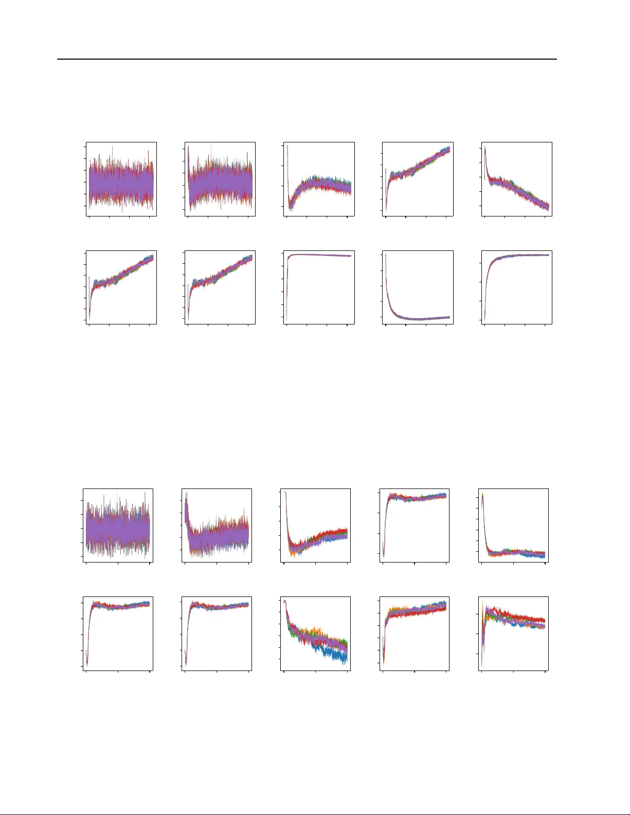
Bullet T rains: Parallelizing T raining of T emporally Pr ecise Spiking Neural Networks T odd Morrill 1 2 Christian Pehle 2 Anthony Zador 2 Abstract Continuous-time, ev ent-nati ve spiking neural net- works (SNNs) operate strictly on spike ev ents, treating spike timing and ordering as the represen- tation rather than an artif act of time discretization. This vie wpoint aligns with biological computation and with the nati v e resolution of e v ent sensors and neuromorphic processors, while enabling com- pute and memory that scale with the number of ev ents. Howe ver , two challenges hinder practical, end-to-end trainable ev ent-based SNN systems: 1) exact char ge–ﬁre–reset dynamics impose inher- ently sequential processing of input spikes, and 2) precise spike times must be solved without time bins. W e address both. First, we use parallel as- sociativ e scans to consume multiple input spikes at once, yielding up to 44x speedups ov er sequen- tial simulation while retaining exact hard-reset dynamics. Second, we implement dif ferentiable spike-time solv ers that compute spike times to machine precision without discrete-time approx- imations or restricti ve analytic assumptions. W e demonstrate the viability of training SNNs us- ing our solutions on four ev ent-based datasets on GPUs. 1. Introduction A commonly cited advantage of spiking neural networks (SNNs) is their ability to operate in an ev ent-based manner , processing information only when spikes occur ( Merolla et al. , 2014 ; Davies et al. , 2018 ). On appropriate neuro- morphic hardware, this implies energy ef ﬁciency , as com- putation only occurs when spikes are present ( Roy et al. , 2019 ; Y ao et al. , 2024 ). At the same time, much SNN research still happens on readily av ailable hardware such as graphical processing units (GPUs) so accelerating this 1 Department of Computer Science, Columbia University , New Y ork, NY , USA 2 Department of Neuroscience, Cold Spring Harbor Laboratory , Cold Spring Harbor, NY , USA. Correspondence to: T odd Morrill < todd@cs.columbia.edu > . Pr eprint. Marc h 17, 2026. 128 256 512 Hidden Layer Size 0 2 4 6 8 10 12 14 Average Batch Runtime (s) 44.27x Speedup Serial Computation Parallel Computation F igure 1. Our parallel method achieves up to 44x speedups over serial processing of spike e vents on se veral ev ent-based datasets while retaining exact hard-reset dynamics. The plot shows results for the Spiking Heidelberg Digits (SHD) dataset. workload (e.g., via parallelization) and mirroring properties of biology and ev ent-based neuromorphic hardware (e.g., precise spike times) ( Carr & K onishi , 1990 ; Thorpe & Gau- trais , 1998 ; Amir et al. , 2017 ; Richter et al. , 2024 ) is an important research direction. In this work, we present a strictly e vent-based SNN system that processes multiple spike e vents in parallel, achie ving signiﬁcant speedups over sequential processing. Second, we present differentiable spike-time solvers that enable machine-precision spik e tim- ing. These two contributions allo w us to take a step toward ev ent-native spiking computation, where preserving con- tinuous spik e times is the objective—both for biological ﬁdelity and for compatibility with neuromorphic sensing and hardware—and where ef ﬁciency follows from operating directly on ev ents. SNNs are challenging to parallelize along the time dimen- sion due to the sequential nature of “charge–ﬁre–reset” dy- namics. After consuming each and e very input spik e, a neuron must determine whether it will produce a spike itself before the next input spike arri ves. Performed naively , SNNs must process one spike at a time, leading to signiﬁcant com- putational bottlenecks on modern parallel hardw are such as graphical processing units (GPU) ( Shrestha & Orchard , 1 Bullet T rains: Parallelizing T raining of T emporally Pr ecise SNNs A B A Computed in parallel 0.000 0.005 0.010 0.015 0.020 0.025 T ime (s) 0.0 0.5 1.0 1.5 2.0 2.5 3.0 State value 0.02031 V th (threshol d) V (membrane potential) I (synaptic current) t V ma x (voltage peak times) Spike time Newton-Raphson T race 0.018 0.019 0.020 0.021 T ime (s) 0 F igure 2. Our contributions visualized—state trajectory of a LIF neuron consuming input spikes in parallel and producing an output spike with our Newton-Raphson solver . A shows the neuron jumping from the initial state s 0 at time 0 (composed of membrane potential and synaptic current) directly to all future states s 1 = f 1 ( s 0 ) , s 2 = f 2 ( s 0 ) , . . . in parallel using associati ve scans. W e use lightweight analytical checks to determine if an output spike will occur in the interval between any consecutiv e pair of input spikes by computing—in parallel— t V max ( s ) , the time of maximum v oltage starting at the interv al’ s left endpoint, and V ( t V max ) the voltage at that time, namely the maximum voltage v alue. The voltage state is hard reset at the spike time. B shows our iterati ve Newton-Raphson solv er ﬁnding the output spike time t ⋆ , computed to machine precision. 2018 ; Engelken , 2023 ; F ang et al. , 2023 ; Li et al. , 2024 ; Zhong et al. , 2024 ; Feng et al. , 2025 ). In the past few years, many methods have been proposed to parallelize spiking dynamics, but they all modify the neuron model in some way , such as removing resets entirely , which can reduce the non-linear expressivity of the neuron and/or deviate from the way biological neurons operate. In this work, we propose a method for parallel training of exact hard-reset spiking dynamics using parallel associa- tiv e scans. The ke y idea is to process input spike trains in chunks, where each chunk is processed in parallel using associativ e scans. Crucially , this is spike-a ware chunking: lightweight analytical checks quickly determine whether a neuron spikes within a chunk and, if so, locate the ﬁrst such spike, allo wing the simulation to jump directly to that time. The next chunk resumes processing input spikes immedi- ately after the output spike. In practice, ev en if a portion of work is discarded, the ov erall speedup relativ e to sequential processing is signiﬁcant because of the parallelism afforded by modern hardware. The result is a parallel system that achiev es up to 44x speedups over sequential processing on sev eral ev ent-based datasets while retaining e xact hard-reset dynamics. A second challenge that arises in strictly event-based SNNs is determining spike times precisely without the use of discrete-time bins. Nearly all SNN implementations to date operate on discrete-time grids ( Bauer et al. , 2023 ; Ham- mouamri et al. , 2024 ; No wotny et al. , 2025 ), which means that neurons are performing computation at every time step, regardless of whether spikes are present. The result of this modeling choice is computation—and often memory usage—that scales with the number of time steps rather than the number of spikes, se verely limiting the number of time steps that can be simulated. T emporal resolution is limited by the time-step size and spike ordering within a time bin cannot be determined ( Bauer et al. , 2023 ) (see Figure 3 ). In contrast, sev eral systems hav e proposed analytical solutions for continuous spike times, but these methods often impose restrictions on the neuron model, such as the relationship between synaptic and membrane time constants in leaky- integrate-and-ﬁre (LIF) neurons ( Mostafa , 2018 ; G ¨ oltz et al. , 2021 ; Engelken , 2023 ). Here, we apply sev eral methods for differentiable spike-time solvers—namely Ne wton-Raphson and Bisection numerical root solv ers—which resolv e spike times to machine pre- cision without the need for discrete-time approximations. This remov es a constraint on SNN systems (e.g., to support heterogeneous time constants ( Perez-Nie ves et al. , 2021 )), facilitates the e xploration of neuro-inspired theories of time- based computation ( Y ang & Zador , 2012 ; Xie et al. , 2024 ), matches the temporal-resolution of event-based sensors and neuromorphic hardware ( M ¨ uller et al. , 2024 ), and enables compute and memory to scale in proportion to the number of spikes. 2 Bullet T rains: Parallelizing T raining of T emporally Pr ecise SNNs 2. Related W ork Parallelizing Spiking Dynamics. Biological neurons go through a “charge–ﬁre–reset” cycle and in the “reset” stage, the neuron’ s membrane potential is set to a baseline v alue ( Hodgkin & Huxle y , 1952 ). It has been ar gued that this hard reset is essential for implementing precise feature detection ( Berry & Meister , 1998 ). The sequential dependency of the “charge–ﬁre–reset” c ycle in simulated Leaky Integrate- and-Fire (LIF) neurons presents a fundamental barrier to parallel training on modern hardware. While sub-threshold dynamics are linear and can be parallelized using associa- tiv e scans—similar to state-space models ( Sch ¨ one et al. , 2025 )—the non-linear spike generation and hard reset in- troduce a sequential dependency that prev ents complete parallelization. Early approaches, such as the Parallel Spik- ing Neuron (PSN), circumvented this “charge–ﬁre–reset” cycle by removing the reset mechanism entirely , ef fecti vely reducing the neuron to a linear ﬁlter solvable via con volu- tions ( Fang et al. , 2023 ). While efﬁcient, this sacriﬁces the non-linear regulation (i.e., “hard reset”) of the membrane potential essential for expressivity and biological ﬁdelity ( Bauer et al. , 2023 ). Subsequent methods like the Parallel Spiking Unit ( Li et al. , 2024 ) and SPikE-SSM ( Zhong et al. , 2024 ) decoupled the reset from integration, b ut rely on “soft reset” mechanisms (linear subtraction) rather than “hard reset” (reset-to-zero). Most recently , Fixed-point Parallel T raining (FPT) attempted to model hard resets via iterativ e scans, yet to guarantee con ver gence of the ﬁx ed-point iter - ation, FPT must relax the discontinuous spike generation into a continuous sigmoid surrogate during the forward pass ( Feng et al. , 2025 ). Consequently , existing parallel meth- ods either fundamentally alter the neuron model (removing resets), assume linearity (soft resets), or solve a relax ed approximation (smoothed dynamics). T o the best of our knowledge, no prior w ork has achie ved parallel acceleration of exact, hard-reset dynamics without approximation. Precise Spike-T ime Solvers. SNN implementations must make two core design choices: 1) whether to use surro- gate gradients or exact gradients, and 2) whether to use a discrete-time grid or operate in continuous time. If exact gradients are coupled with continuous time, a third deci- sion must be made: whether to use analytical spik e-time solutions or numerical spike-time solv ers. Surrogate gradi- ent (SG) methods ( Shrestha & Orchard , 2018 ; Neftci et al. , 2019 ) are inextricably linked to discrete time steps. W e therefore focus our discussion on exact gradient methods to retain machine-precision spike times. Many exact gradient methods to date operate on discrete-time grids, where spike times are approximated to the nearest time step ( Bauer et al. , 2023 ; Now otny et al. , 2025 ; M ´ esz ´ aros et al. , 2025 ). Se veral methods hav e used analytical solutions for continuous spike times, but these methods often impose restrictions on the 0.002 0.003 T ime (s) 0.0 0.5 1.0 1.5 2.0 2.5 Membrane Potential Quantization Error Spike T ime: 0.0027s Spike T ime: 0.0021s T ime Grid Threshold Spike F igure 3. Discrete-time binning causes quantization errors and loses spike ordering. Here, two spikes occurring at dif ferent times (0.0021s and 0.0027s) both round to 0.003s, making them indistin- guishable to downstream neurons. neuron model ( Boht ´ e et al. , 2000 ; Mostafa , 2018 ; G ¨ oltz et al. , 2021 ; Engelken , 2023 ). Newton-Raphson and Bisec- tion methods have been proposed for ﬁnding spike times in neural simulations ( D’Haene et al. , 2009 ) but have not been explicated for training SNNs with gradient descent on large-scale tasks on GPUs. 1 In this work, we demonstrate the effecti veness of training SNNs using numerical spike- time solvers based on the Ne wton-Raphson and Bisection methods, which can be applied to a wide v ariety of neuron models—without restricti ve assumptions—while w orking with exact gradients in continuous time. 3. Event-Based Spiking Neural Networks Here we describe our proposed methods for building e vent- based spiking neural netw orks that 1) process multiple input spike events in parallel while maintaining temporal causality with exact hard-reset dynamics, and 2) determine spike times precisely using differentiable numerical spike-time solvers. 3.1. LIF Neurons Our SNNs are built from current-based leaky-inte grate-and- ﬁre (LIF) neurons ( Rotter & Diesmann , 1999 ; Gerstner & Kistler , 2002 ), one of the most popular neurons in the SNN community ( W underlich & Pehle , 2021 ; G ¨ oltz et al. , 2021 ; Now otny et al. , 2025 ; Hammouamri et al. , 2024 ; M ´ esz ´ aros et al. , 2025 ), with the follo wing sub-threshold dynamics— the dynamics between spikes—on the synaptic input current 1 W underlich & Pehle ( 2021 ) used the T oms 748 ( Alefeld et al. , 1995 ) root solving algorithm on a CPU. 3 Bullet T rains: Parallelizing T raining of T emporally Pr ecise SNNs T ime Weight Chunk 1 Chunk 2 Chunk 3 Repeated Work Spike — — Input Queue Consuming Neuron Output Queue Spike F igure 4. An example input queue feeding a neuron and producing an output queue. The input chunk size is 4 spikes, which means 4 input spikes are consumed in parallel. After consuming 3 input spikes in chunk 1, the neuron produces an output spike. The work done to consume the 4th input spike in chunk 1 is discarded, and the next chunk resumes processing input spik es immediately after the output spike time. I ( t ) and membrane potential V ( t ) . τ m dV dt = − V ( t ) + I ( t ) (1) τ s dI dt = − I ( t ) (2) where τ m and τ s are the membrane and synaptic time con- stants, respecti vely . Closed-form solutions for these dif fer- ential equations are provided in Appendix Section A . A LIF neuron emits a spike at time t when the membrane potential crosses a threshold V th (i.e., V ( t ) ≥ V th ), as de- picted in Figure 2 A and then resets to a reset potential V reset , which is set to 0 in this work. Neurons indexed by i that are downstream of the spiking neuron j hav e their synap- tic input currents incremented by the synaptic weights w ij , which are learned during training. W e also introduce learn- able synaptic delays d ij , which simulate the time a spike would take to be transmitted from one neuron to the next. The synaptic input current is then I ( t ) ← I ( t ) + X k w ij δ ( t − ( t k + d ij )) (3) where t k is the time of the k th spike from neuron j and δ ( t ) is the Dirac delta function. 3.2. Event-Driv en Implementation with Exact Gradients W e implement our SNN in JAX in an e vent-based manner . The core idea of an ev ent-based SNN is that if for each neuron in the system you know which of two events will happen ﬁrst, namely whether a neuron should ﬁrst consume an incoming spike or ﬁrst emit a spike itself, then you can directly advance the simulation to the appropriate ev ent. This highlights the distinction between our ev ent-dri ven approach and discrete time-stepped approaches, which sim- ulate the entire network’ s state (i.e., membrane potential and synaptic input current) at every discrete point in time. W e train the model’ s parameters via gradient descent using exact gradients. The key idea for being able to use exact 4 6 8 10 12 14 Input Weight w 0.002 0.004 0.006 0.008 0.010 0.012 0.014 Spike Time t ( w ) (seconds) Continuous Spike T ime Discrete Spike T ime F igure 5. Spike time as a function of synaptic weight for different time constant conﬁgurations. Discrete time approximation with ∆ t = 1 ms div erges from the ground truth spike time at nearly all weight values, while our method closely tracks the ground truth spike time. gradient descent is that spike times a re dif ferentiable func- tions of the SNN’ s synaptic weights and delay parameters ( Mostafa , 2018 ; W underlich & Pehle , 2021 ). Intuiti vely , if a weight onto a postsynaptic neuron is increased, it has the effect of charging the neuron up faster , and in turn ac- celerating the spiking time of the postsynaptic neuron (see Figure 5 ). The event-based exact gradient approach is in contrast to surrogate gradient methods, which use a discrete time-stepped approach and lose the ability to disambiguate spikes within the step windo w (see Figure 3 ) and therefore, machine-precision spike times. 3 . 2 . 1 . P A R A L L E L P R O C E S S I N G O F S P I K E E V E N T S Processing incoming spikes to a LIF neuron one-by-one be- comes a computational bottleneck because it scales linearly with the number of input spikes as O ( N ) where N is the number of spikes to be processed. State-space models simi- larly face this problem due to their recurrent nature. One so- 4 Bullet T rains: Parallelizing T raining of T emporally Pr ecise SNNs lution to this problem is to parallelize computation along the time-dimension through the use of an associativ e scan. The key observation is to note that sub-threshold transitions of the LIF neuron state—its voltage and input current—can be expressed as af ﬁne maps, which admit an associativ e opera- tion on these maps. These af ﬁne maps allo w one to compute a transition from an initial voltage and input current state, s 0 = [ V 0 , I 0 ] ⊤ , to all neuron states in the future at each input spike time, s 1 = [ V 1 , I 1 ] ⊤ , . . . , s N = [ V N , I N ] ⊤ . Im- portantly , once these afﬁne maps are computed, we can consume all input spikes in parallel using an associati ve scan and directly advance the neuron to any intermediate state (i.e., any state s i for i ∈ [1 , N ] ) without having to sequentially process all previous spikes. T o understand how we deriv e the associative operator, it is instructive to see how the neuron’ s state transitions from the ﬁrst state s 0 to the second state s 1 after consuming the ﬁrst input spik e. Let C m = exp ( − t/τ m ) and C s = exp ( − t/τ s ) . The af ﬁne map f 1 : s 0 → s 1 to transition the neuron from state i = 0 to state i = 1 , for example, is gi ven by  V 1 I 1  | {z } s 1 =  C m τ s τ m − τ s [ C m − C s ] 0 C s  | {z } M 1  V 0 I 0  | {z } s 0 +  0 w  |{z} b 1 (4) where we have denoted M 1 as the matrix that advances the neuron’ s state, and b 1 as the vector that injects a new spike into the neuron with weight w . Equation 4 follows from closed-form equations for our system (see Appendix Equations 19 , 20 ) and Equation 3 . Note that M 1 is deﬁned by the time between the starting time, t 0 , and the spike time t 1 (i.e., t = t 1 − t 0 ). Examining the composition of two consecuti ve af ﬁne maps (i.e., consuming 2 consecuti ve input spik es) sho ws that com- posing such maps yields another afﬁne map, which leads us to an associati ve operator commonly called Combine in parallel scan algorithms (lemma and proof in Appendix Section B ). The important point is that Combine allows us to mak e use of the jax.lax.associative scan function, which computes a sequence of K afﬁne maps, f 1 , f 2 , . . . , f K , with parallel depth O (log K ) — exponentially faster than the O ( K ) serial approach because operations can be combined in a tree-like fashion ( Blelloch , 1990 ). Once we have these afﬁne maps, we can produce the sequence ( s 0 , s 1 , s 2 , . . . , s K ) in parallel. Since a neuron can produce a spike at any point after consuming a spike (see Figure 2 ) and we would lik e to a v oid discarding excessi ve amounts of work, we consume input spikes in chunks, where each chunk contains K input spikes that are processed in parallel using the associati ve scan approach, which implies a parallel compute graph depth of O ( C log K ) where C is the number of chunks. Between each pair of spikes in a chunk, we determine (see Section 3.2.2 ) if an output spike will occur in that interv al. If the neuron spikes, we discard any 32 64 128 256 Chunk Size 0.25 0.50 0.75 1.00 1.25 1.50 1.75 2.00 Average Batch Runtime (s) Batch-Hidden Size 32-128 32-256 32-512 64-128 64-256 64-512 128-128 128-256 128-512 F igure 6. T raining time per batch as we vary chunk size on the SHD dataset with hidden dimensions ranging from 128 to 512 and batch size ranging from 32 to 128. A verages are taken over 100 batches. work done within the chunk after the output spike time and revis it those input spikes on the ne xt iteration (see Figure 4 ). Discarding work refers only to intermediate computations after the ﬁrst within-chunk output spike; the event order and hard resets for processed spikes are unchanged. F or efﬁcient GPU just-in-time (JIT) compilation, we pre-specify a ﬁxed compute budget—the number of chunks C and a per-neuron output-spike cap S max (Appendix Section E.2 )— so all processed spikes follow exact hard-reset semantics, though if the cap activ ates some input spikes may remain unprocessed within the compiled budget. In practice, we consume ≈ 96% of SSC input spikes in layer 1 ( S (1) max = 42 ) and nearly 100% in layer 2 ( S (2) max = 28 ) (Appendix Fig- ure 11 ). A spike-count re gularizer (Appendix Section E.1 ) keeps ﬁring sparse, maintaining high consumption without sacriﬁcing accuracy . 3 . 2 . 2 . D I FF E R E N T I A B L E S P I K E - T I M E S O L V E R S A core capability of any SNN system is to detect the times at which a neuron produces spikes. This in volv es solving for t ⋆ , the time at which the membrane potential V ( t ) crosses the threshold V th . W e use root solvers, which keep our system ev ent-based and temporally precise. A spik e occurs at the time at which the following relation R is satisﬁed R ( V 0 , I 0 , V th , t ) = V ( V 0 , I 0 , t ) − V th = 0 (5) namely when the membrane potential V is equal to the threshold, V th , where V ( V 0 , I 0 , t ) is the membrane potential at time t giv en initial conditions V 0 and I 0 (see Equation 19 ). For brevity , we denote the neuron’ s initial state and 5 Bullet T rains: Parallelizing T raining of T emporally Pr ecise SNNs 2 4 6 8 10 Iteration −0.0020 −0.0015 −0.0010 −0.0005 0.0000 0.0005 0.0010 Spike T ime Error (s) Newton-Raphson Bisection F igure 7. Conv ergence of the Newton-Raphson and Bisection solvers to wards the ground truth spike time. threshold as p = ( V 0 , I 0 , V th ) , allo wing us to write the spike condition compactly as R ( p , t ( p )) = 0 , where t ( p ) is the spike time as a function of these parameters. There are many choices of root solvers for recovering the output spike time t ⋆ . T wo ef fecti ve options are Newton- Raphson, which iterati vely reﬁnes the spike time (see Fig- ure 2 B), and Bisection, which repeatedly bisects an interval containing the spike. W e describe both in Appendix Sec- tion D , but primarily use Newton-Raphson due to its fast con vergence rate (see Figure 7 ). A ﬁnal challenge is computing gradients of the spike time t ⋆ with respect to the neuron’ s parameters p = ( V 0 , I 0 , V th ) . Rather than differentiating through the iterati ve solver steps, we use the Implicit Function Theorem ( Mostaf a , 2018 ; Chen et al. , 2018 ; W underlich & Pehle , 2021 ) to compute these gradients directly . In particular , we aim to compute the Jacobian ∂ t ⋆ /∂ p . W e describe the deri v ation in Appendix Section D.3 . 3.3. T ranslating Spike T rains to Class Logits Our model’ s ﬁnal layer is composed of N cls weighted leaky integrators (i.e., no spiking non-linearity) ( No wotny et al. , 2025 ), one for each class in the classiﬁcation task, that accumulate incoming spikes over time, which we directly use as logits in a cross-entropy loss function. W e can use the associative operator Combine , to implement a Leak y Integrator (LI) neuron, which follows the same dynamics as the LIF neuron, except it does not produce output spikes. Logits are computed via the following inte gral Z t = τ max t =0 e − t/τ LI V ( t ) dt. (6) where τ max is some prespeciﬁed maximum and τ LI is the exponential time constant. The intuition behind this vari- 32 64 128 32 64 128 32 64 128 0 2 4 6 8 10 12 14 Average Batch Runtime (s) 44.27x 29.44x 19.19x 30.75x 20.14x 13.63x 20.59x 13.75x 7.95x 128 256 512 Batch Size Hidden Layer Size Serial Computation Parallel Computation F igure 8. Speedup of our parallel SNN implementation ov er a sequential ev ent-based SNN implementation with exact hard-reset dynamics on the SHD dataset as we vary the hidden dimension and batch size. The model architecture uses 2 feedforward hidden layers and delays. A verages are taken o ver 100 batches (forward and backward pass) ov er 3 runs and chunk size is set to 128. ant is that spikes that arrive earlier at the output neurons are weighted more heavily than spik es that arri ve later . W e provide complete closed-form equations for computing this integral in an event-based manner in the Appendix. Further - more, complete training details, including hyperparameters, spike-count regularizer speciﬁcation, dataset preprocessing, and other implementation details are provided in the Ap- pendix. 4. Experiments Our experiments probe se veral research questions: 1) How much speedup can be achie ved by processing input spikes in parallel using associati ve scans while maintaining exact hard-reset dynamics? 2) Can numerical spike-time solv ers such as Newton-Raphson be used to train SNNs on ev ent- based datasets? 3) How does discretizing spik e times into time bins impact classiﬁcation accuracy on a task requiring sub-millisecond precision? Our e xperiments are performed on four e vent-based datasets, including the Spiking Heidelberg Digits (SHD) dataset ( Cramer et al. , 2022 ), the Spiking Speech Commands (SSC) dataset ( Cramer et al. , 2022 ), the latenc y-encoded MNIST dataset, and the Y in-Y ang (YY) dataset ( Kriener et al. , 2022 ). Our model architecture is composed of fully connected lay- ers of LIF neurons. The output layer is composed of N cls leaky integrator neurons, where N cls is the number of classes in the dataset. Complete training details are provided in the Appendix. W e compare our method against a sequential ev ent-based SNN implementation with exact hard-reset dy- namics, which consumes input spikes one-by-one and after each spike, checks if the neuron will produce an output 6 Bullet T rains: Parallelizing T raining of T emporally Pr ecise SNNs T able 1. Classiﬁcation accuracy comparison on e vent-based datasets. Model architectures are deﬁned by number of layers and connecti vity pattern (F for feedforw ard, R for recurrent), number of hidden units (H), and use of delays (D) (e.g., 2F512HD means 2 layers, feedforward connectivity , 512 hidden units, and use of delays). N is the number of spikes processed by a single neuron and T is the number of time steps in the simulation. Our metrics are av eraged ov er 5 random seeds and standard de viation is reported in parentheses. Dataset Model Exact Gradients Continuous Spike T imes Parallelized Compute Depth Memory Accuracy MNIST 1F350H, τ m = 2 τ s ( G ¨ oltz et al. , 2021 ) ✓ ✓ x O ( N ) O ( N ) 97.20 (0.10) 1F350H ( W underlich & Pehle , 2021 ) ✓ ✓ x O ( N ) O ( N ) 97.60 (0.10) 1F350H (Ours) ✓ ✓ ✓ O ( C log K ) O ( N ) 98.04 (0.07) SHD 2F256HD ( Hammouamri et al. , 2024 ) x x x O ( T ) O ( T ) 95.07 (0.24) 2F512HD ( M ´ esz ´ aros et al. , 2025 ) ✓ x x O ( T ) O ( N ) 93.10 2F256HD (Ours) ✓ ✓ ✓ O ( C log K ) O ( N ) 94.78 (0.56) 2F512HD (Ours) ✓ ✓ ✓ O ( C log K ) O ( N ) 95.10 (0.20) SSC 2F512HD ( Hammouamri et al. , 2024 ) x x x O ( T ) O ( T ) 80.69 (0.21) 2F512HD ( M ´ esz ´ aros et al. , 2025 ) ✓ x x O ( T ) O ( N ) 76.10 (1.00) 2F512HD (Ours) ✓ ✓ ✓ O ( C log K ) O ( N ) 77.35 (0.23) spike before the ne xt input spike arri ves. If so, the neuron produces the output spike and resets its membrane poten- tial to zero before continuing to consume input spikes. W e report training speed compared to this serial baseline and explore ho w the chunk size (i.e., the number of input spikes processed in parallel) impacts training speed. W e also com- pare our method’ s properties and classiﬁcation accuracy to those of prior works that use discrete-time approximations, analytical spike-time solutions, and surrogate gradients. 4.1. Parallel Associativ e Scan Speedups & Optimal Chunk Size W e measure the training time per batch of our parallel SNN implementation against a sequential/serial ev ent-based SNN implementation with exact hard-reset dynamics. W e vary the batch size, number of hidden units, and chunk size (i.e., the number of input spikes processed in parallel) to understand how these parameters impact speedup. Here, we report results on the SHD dataset and report SSC results in Appendix Section F . In Figure 8 , we ﬁnd that our parallel SNN implementa- tion achiev es up to 44x speedup over the sequential base- line. At larger batch sizes and larger hidden dimensions, we still observe lar ge speedups, particularly in absolute terms, where sequential training slows do wn dramatically . W e also ﬁnd that chunk size plays a signiﬁcant role in maxi- mizing throughput as seen in Figure 6 . W e ﬁnd that the optimal chunk size is determined by a combination of the number of hidden units and batch size. Larger chunk sizes allow for more parallelism, but also require moving more data—taxing memory bandwidth—and scheduling more work, which can lead to diminishing returns. W e ﬁnd that chunk size 128 works well across a variety of batch sizes and hidden dimensions. Larger chunk sizes may also lead to more wasted computation, since more work is discarded when a neuron spikes early in the chunk. Howe ver , we ﬁnd that this effect is manageable in practice since neurons tend to spike sparsely relati ve to the number of input spikes they receiv e. W e quantify the percentage of work retained in Appendix Section G . 4.2. Classiﬁcation Accuracy T able 1 summarizes k ey attrib utes of different methods and their classiﬁcation accuracy on e vent-based datasets. MNIST . W e note the fav orable computational scaling properties of our method, which has compute depth O ( C log K ) due to our use of parallel associative scans, compared to either O ( N ) or O ( T ) for other methods, where T is the number of discrete time steps in the simulation. W e also note an improved classiﬁcation accuracy of 98.04% for the same parameter count compared to prior works that use exact gradients with analytical spike-time solutions where the membrane and synaptic time constants are restricted to hav e the relation τ m = 2 τ s ( G ¨ oltz et al. , 2021 ). SHD and SSC. W e compare against methods that use ex- act gradients with discrete spike times ( M ´ esz ´ aros et al. , 2025 ) and surrogate gradients with a discrete time grid ( Hammouamri et al. , 2024 ) (see Figure 5 for a visualization of ho w discretization af fects the smoothness of the opti- mization landscape). Compared to M ´ esz ´ aros et al. ( 2025 ), we ﬁnd that our method’ s classiﬁcation accuracy performs fa vorably on both the SHD and SSC datasets, conﬁrming the feasibility of using numerical spike-time solvers in SNN training and the potential advantages of continuous-time methods. 2 W e also note that our method not only operates ov er continuous spike times, b ut also operates over contin- 2 Best reported accuracy from M ´ esz ´ aros et al. ( 2025 ) on SHD is 93.24 (1.0), though we benchmark comparable architectures. 7 Bullet T rains: Parallelizing T raining of T emporally Pr ecise SNNs 0.000 0.001 0.002 0.003 0.004 0.005 Quantization T ime Step (s) 30 40 50 60 70 80 90 T est Accuracy (%) F igure 9. Impact of temporal discretization on Y in-Y ang clas- siﬁcation. W e trained our method under different discrete-time constraints by quantizing spike times to multiples of ∆ t during training and testing. Accuracy degrades signiﬁcantly as ∆ t in- creases, dropping to near -chance ( 33% ) at ∆ t ≥ 2 ms. Continuous spike times ( ∆ t → 0 , our standard method) maintain the highest accuracy , demonstrating that discrete-time methods would require ∆ t ≪ 1 ms—incurring substantial computational costs—to pre- serve temporal information. uous delays, whereas M ´ esz ´ aros et al. ( 2025 ) use discrete delays. Notably , our system supports continuous delays and multiple spikes per neuron—an important distinction from other recent ev ent-based continuous time SNNs with delays ( G ¨ oltz et al. , 2025 ) (see Appendix Figure 11 for observed per-layer spik e counts during training). Our method’ s accuracy is comparable to that of Ham- mouamri et al. ( 2024 ) on the SHD dataset and lower on the SSC dataset. Hammouamri et al. ( 2024 )’ s use of sur- rogate gradients leads to a loss of machine-precision spik e times, O ( T ) compute/memory (vs. our O ( C log K ) com- pute, O ( N ) memory), and binned input spike trains. W e use full spike trains with no loss of temporal resolution. W e note that current standard benchmarks (SHD, SSC) are solvable via rate-coding, which fav ors the smoothing properties of surrogate gradients ( Ma et al. , 2025 ). While benchmarks re- quiring strict spike-timing codes are emerging, to our kno wl- edge there is not yet a widely adopted community-standard large-scale benchmark whose performance rob ustly depends on strict spike-timing codes. Our method provides the nec- essary approach to train on such future datasets efﬁciently . 4.3. Impact of Discretization on T emporal Coding T asks T o demonstrate the limitations of discrete-time methods on temporal coding tasks, we created a barn owl-inspired interaural time difference (ITD) task using the Y in-Y ang dataset ( Kriener et al. , 2022 ). Each sample consists of 5 input spikes arriving within 2ms, where spike times en- code the ( x, y ) position on the Y in-Y ang symbol. The 3- way classiﬁcation (yin, yang, dot) requires sub-millisecond discrimination—analogous to barn o wl sound localization ( Carr & K onishi , 1990 ). W e trained our method under dif- ferent discrete-time constraints to simulate what discrete- time methods would experience. For each time step size ∆ t , we quantized all spike times to the nearest multiple of ∆ t during training and testing. Figure 9 shows that ac- curacy de grades signiﬁcantly as ∆ t increases, dropping to near-chance le vels ( 33% ) at ∆ t ≥ 2 ms. Our method with continuous spike times maintains the highest accurac y . This demonstrates that achieving sub-millisecond precision (e.g., ∆ t = 0 . 1 ms) would require discrete-time methods to incur 10 × higher memory and computation costs compared to 1ms bins, whereas our continuous-time approach achie ves this precision without such penalties. 5. Discussion This work opens up several av enues for future research. One potential direction is to e xplore the application of our method to more complex SNN architectures, such as con- volutional or recurrent networks. Recurrence in particular poses interesting challenges for parallel processing on mod- ern hardware, such as GPUs, because the input queues to each neuron are dynamic. While data structures such as heaps/priority queues are sensible choices to consider , they are very indexing and memory access intensi ve, which may make them ill-suited for GPU architectures ( Engelken , 2023 ; Landsmeer et al. , 2025 ). Additionally , now that we have demonstrated the effecti veness of using numerical spike- time solvers in SNN training, we can explore a wider range of neuron models, which may lead to improv ed performance on ev ent-based tasks. Finally , ev aluating the impact of train- ing with precise spike times on do wnstream deployment to temporally precise neuromorphic hardware is an exciting direction and is left for future work. This paper presents a novel combination of methods that unlocks ﬂexible and ef ﬁcient training of temporally pre- cise spiking neural networks on modern parallel hardware, speciﬁcally via parallel associative scans—while main- taining hard-reset dynamics—and differentiable spik e-time solvers. W e demonstrate signiﬁcant speedups in training time ov er sequential ev ent-based SNN approaches. W e also demonstrate that our numerical spike-time solver is capable of machine precision spike times, which enables in vestiga- tions into how the brain might lev erage spike timing and ordering for computation, compatibility with high resolu- tion sensors and neuromorphic hardware, and computing on an ev ent-by-event basis, where memory and compute scale with the number of spikes processed rather than the number of discrete time steps simulated. Furthermore, we enable continuous spike times while remo ving the restriction that 8 Bullet T rains: Parallelizing T raining of T emporally Pr ecise SNNs the neuron model must ha ve an analytical spike-time solu- tion. Our method achiev es strong classiﬁcation accuracy on event-based datasets compared to prior works that use discrete-time approximations, indicating the viability of us- ing numerical spike-time solvers in SNN training. Software and Data Our codebase will be made publicly av ailable upon publication. The datasets used in this w ork are publicly av ailable at the following URLs: SHD and SSC datasets https://tonic.readthedocs.io/en/latest/ datasets.html , and MNIST dataset https:// docs.pytorch.org/vision/main/generated/ torchvision.datasets.MNIST.html . Acknowledgements W e thank Richard Zemel for helpful discussions and feed- back on the manuscript. This work was supported by the funds provided by the National Science F oundation and by DoD OUSD (R&E) under Cooperative Agreement PHY - 2229929 (The NSF AI Institute for Artiﬁcial and Natu- ral Intelligence). This w ork was also performed with as- sistance from the US National Institutes of Health Grant S10OD028632-01. Impact Statement This paper presents work whose goal is to advance the ﬁeld of Machine Learning. There are many potential societal consequences of our work, none which we feel must be speciﬁcally highlighted here. References Alefeld, G. E., Potra, F . A., and Shi, Y . Algorithm 748: Enclosing zeros of continuous functions. A CM T rans. Math. Softw . , 21(3):327–344, September 1995. ISSN 0098-3500. doi: 10.1145/210089.210111. Amir , A., T aba, B., Berg, D., Melano, T ., McKinstry , J., Di Nolfo, C., Nayak, T ., Andreopoulos, A., Garreau, G., Mendoza, M., Kusnitz, J., Debole, M., Esser , S., Delbruck, T ., Flickner , M., and Modha, D. A Low Power, Fully Event-Based Gesture Recognition System. In 2017 IEEE Confer ence on Computer V ision and P at- tern Recognition (CVPR) , pp. 7388–7397, July 2017. doi: 10.1109/CVPR.2017.781. Bauer , F . C., Lenz, G., Haghighatshoar , S., and Sheik, S. EXODUS: Stable and efﬁcient training of spiking neural networks. F r ontiers in Neur oscience , 17, February 2023. ISSN 1662-453X. doi: 10.3389/fnins.2023.1110444. Berry , M. J. and Meister, M. Refractoriness and Neural Precision. J ournal of Neuroscience , 18(6):2200–2211, March 1998. ISSN 0270-6474, 1529-2401. doi: 10.1523/ JNEUR OSCI.18- 06- 02200.1998. Blelloch, G. E. Preﬁx Sums and Their Applications. T ech- nical Report T echnical Report CMU-CS-90-190, School of Computer Science, Carnegie Mellon Uni versity , 1990. Boht ´ e, S., K ok, J., and Poutr ´ e, H. L. Spik eProp: Backpropa- gation for networks of spiking neurons. In The Eur opean Symposium on Artiﬁcial Neural Networks , 2000. Carr , C. E. and Konishi, M. A circuit for detection of interaural time dif ferences in the brain stem of the barn o wl. The J ournal of Neur oscience: The Of ﬁcial Journal of the Society for Neur oscience , 10(10):3227–3246, October 1990. ISSN 0270-6474. doi: 10.1523/JNEUR OSCI. 10- 10- 03227.1990. Chen, R. T . Q., Rubanov a, Y ., Bettencourt, J., and Duvenaud, D. Neural ordinary dif ferential equations. In Pr oceedings of the 32nd International Conference on Neural Informa- tion Pr ocessing Systems , NIPS’18, pp. 6572–6583, Red Hook, NY , USA, December 2018. Curran Associates Inc. Cramer , B., Stradmann, Y ., Schemmel, J., and Zenke, F . The Heidelberg Spiking Data Sets for the System- atic Evaluation of Spiking Neural Networks. IEEE T ransactions on Neural Networks and Learning Systems , 33(7):2744–2757, July 2022. ISSN 2162-2388. doi: 10.1109/TNNLS.2020.3044364. Davies, M., Srini v asa, N., Lin, T .-H., Chinya, G., Cao, Y ., Choday , S. H., Dimou, G., Joshi, P ., Imam, N., Jain, S., Liao, Y ., Lin, C.-K., Lines, A., Liu, R., Mathaikutty , D., McCoy , S., P aul, A., Tse, J., V enkataramanan, G., W eng, Y .-H., W ild, A., Y ang, Y ., and W ang, H. Loihi: A Neu- romorphic Manycore Processor with On-Chip Learning. IEEE Micr o , 38(1):82–99, January 2018. ISSN 1937- 4143. doi: 10.1109/MM.2018.112130359. D’Haene, M., Schrauwen, B., V an Campenhout, J., and Stroobandt, D. Accelerating Event-Dri ven Simulation of Spiking Neurons with Multiple Synaptic T ime Con- stants. Neural Computation , 21(4):1068–1099, April 2009. ISSN 0899-7667. doi: 10.1162/neco.2008. 02- 08- 707. Engelken, R. SparseProp: Efﬁcient Event-Based Simula- tion and Training of Sparse Recurrent Spiking Neural Networks. Advances in Neural Information Pr ocessing Systems , 36:3638–3657, December 2023. Fang, W ., Y u, Z., Zhou, Z., Chen, D., Chen, Y ., Ma, Z., Masquelier , T ., and T ian, Y . Parallel spiking neurons with high ef ﬁciency and ability to learn long-term dependen- cies. In Pr oceedings of the 37th International Confer ence 9 Bullet T rains: Parallelizing T raining of T emporally Pr ecise SNNs on Neur al Information Pr ocessing Systems , NIPS ’23, pp. 53674–53687, Red Hook, NY , USA, December 2023. Curran Associates Inc. Feng, W ., Gao, X., Du, W ., Shi, H., Zhao, P ., W u, P ., and Miao, C. Efﬁcient Parallel T raining Methods for Spik- ing Neural Networks with Constant T ime Comple xity . In F orty-Second International Confer ence on Machine Learning , June 2025. Gerstner , W . and Kistler , W . M. Spiking Neur on Models Single Neur ons, P opulations, Plasticity . Cambridge Uni- versity Press, 2002. G ¨ oltz, J., Kriener , L., Baumbach, A., Billaudelle, S., Bre- itwieser , O., Cramer , B., Dold, D., Kungl, A. F ., Senn, W ., Schemmel, J., Meier , K., and Petrovici, M. A. Fast and energy-ef ﬁcient neuromorphic deep learning with ﬁrst-spike times. Natur e Machine Intelligence , 3(9): 823–835, September 2021. ISSN 2522-5839. doi: 10.1038/s42256- 021- 00388- x. G ¨ oltz, J., W eber , J., Kriener, L., Billaudelle, S., Lak e, P ., Schemmel, J., Payv and, M., and Petrovici, M. A. Del- Grad: Exact event-based gradients for training delays and weights on spiking neuromorphic hardware. Natur e Communications , 16(1):8245, September 2025. ISSN 2041-1723. doi: 10.1038/s41467- 025- 63120- y. Hammouamri, I., Khalfaoui-Hassani, I., and Masquelier , T . Learning Delays in Spiking Neural Networks using Dilated Con volutions with Learnable Spacings. In Inter- national Confer ence on Learning Representations , 2024. Hodgkin, A. L. and Huxley , A. F . A quantitati ve description of membrane current and its application to conduction and excitation in nerve. The J ournal of Physiology , 117 (4):500–544, 1952. ISSN 1469-7793. doi: 10.1113/ jphysiol.1952.sp004764. Kingma, D. P . and Ba, J. Adam: A Method for Stochastic Optimization, December 2014. Kriener , L., G ¨ oltz, J., and Petrovici, M. A. The Y in-Y ang dataset, January 2022. Landsmeer , L. P . L., Mov ahedin, A., Hamdioui, S., and Strydis, C. EventQueues: Autodifferentiable spik e ev ent queues for brain simulation on AI accelerators, December 2025. Li, Y ., Sun, Y ., He, X., Dong, Y ., Zhao, D., and Zeng, Y . Parallel Spiking Unit for Efﬁcient Training of Spiking Neural Networks, June 2024. Loshchilov , I. and Hutter , F . Decoupled W eight Decay Regularization. In International Confer ence on Learning Repr esentations , September 2018. Ma, C., Chen, X., Li, Y ., Y ang, Q., W u, Y ., Li, G., P an, G., T ang, H., T an, K. C., and W u, J. Spiking Neural Net- works for T emporal Processing: Status Quo and Future Prospects, February 2025. Merolla, P . A., Arthur , J. V ., Alv arez-Icaza, R., Cassidy , A. S., Sawada, J., Akop yan, F ., Jackson, B. L., Imam, N., Guo, C., Nakamura, Y ., Brezzo, B., V o, I., Esser , S. K., Appuswamy , R., T aba, B., Amir , A., Flickner, M. D., Risk, W . P ., Manohar, R., and Modha, D. S. A million spiking-neuron integrated circuit with a scalable com- munication network and interface. Science , 345(6197): 668–673, August 2014. doi: 10.1126/science.1254642. M ´ esz ´ aros, B., Knight, J. C., and Nowotn y , T . Efﬁcient e vent- based delay learning in spiking neural networks. Natur e Communications , 16(1):10422, November 2025. ISSN 2041-1723. doi: 10.1038/s41467- 025- 65394- 8. Mostafa, H. Supervised Learning Based on T emporal Coding in Spiking Neural Networks. IEEE T ransac- tions on Neural Networks and Learning Systems , 29 (7):3227–3235, July 2018. ISSN 2162-2388. doi: 10.1109/TNNLS.2017.2726060. M ¨ uller , E., Althaus, M., Arnold, E., Spilger , P ., Pehle, C., and Schemmel, J. Jaxsnn: Event-dri ven Gradient Es- timation for Analog Neuromorphic Hardware, January 2024. Neftci, E. O., Mostafa, H., and Zenke, F . Surrogate Gra- dient Learning in Spiking Neural Networks: Bringing the Po wer of Gradient-Based Optimization to Spiking Neural Networks. IEEE Signal Pr ocessing Ma gazine , 36(6):51–63, Nov ember 2019. ISSN 1558-0792. doi: 10.1109/MSP .2019.2931595. Now otny , T ., T urner , J. P ., and Knight, J. C. Loss shaping en- hances exact gradient learning with Eventprop in spiking neural networks. Neur omorphic Computing and Engi- neering , 5(1):014001, January 2025. ISSN 2634-4386. doi: 10.1088/2634- 4386/ada852. Perez-Nie ves, N., Leung, V . C. H., Dragotti, P . L., and Good- man, D. F . M. Neural heterogeneity promotes robust learn- ing. Natur e Communications , 12(1):5791, October 2021. ISSN 2041-1723. doi: 10.1038/s41467- 021- 26022- 3. Press, W . H., T eukolsk y , S. A., V etterling, W . T ., and Flan- nery , B. P . Numerical Recipes 3rd Edition: The Art of Scientiﬁc Computing . Cambridge University Press, USA, 3 edition, August 2007. ISBN 978-0-521-88068-8. Richter , O., W u, C., Whatley , A. M., K ¨ ostinger , G., Nielsen, C., Qiao, N., and Indi veri, G. D YN AP-SE2: A scalable multi-core dynamic neuromorphic asynchronous spiking neural network processor . Neuromorphic Computing and 10 Bullet T rains: Parallelizing T raining of T emporally Pr ecise SNNs Engineering , 4(1):014003, January 2024. ISSN 2634- 4386. doi: 10.1088/2634- 4386/ad1cd7. Rotter , S. and Diesmann, M. Exact digital simulation of time-in variant linear systems with applications to neu- ronal modeling. Biological Cybernetics , 81(5):381–402, Nov ember 1999. ISSN 1432-0770. doi: 10.1007/ s004220050570. Roy , K., Jaiswal, A., and Panda, P . T o wards spike-based ma- chine intelligence with neuromorphic computing. Natur e , 575(7784):607–617, Nov ember 2019. ISSN 1476-4687. doi: 10.1038/s41586- 019- 1677- 2. Sch ¨ one, M., Sushma, N. M., Zhuge, J., Mayr , C., Subra- money , A., and Kappel, D. Scalable Event-by-Ev ent Processing of Neuromorphic Sensory Signals With Deep State-Space Models. In Proceedings of the Interna- tional Conference on Neur omorphic Systems , ICONS ’24, pp. 124–131, Arlington, V irginia, USA, October 2025. IEEE Press. ISBN 979-8-3503-6865-9. doi: 10.1109/ICONS62911.2024.00026. Shrestha, S. B. and Orchard, G. SLA YER: Spike Layer Error Reassignment in T ime. In Advances in Neural Informa- tion Pr ocessing Systems , volume 31. Curran Associates, Inc., 2018. Thorpe, S. and Gautrais, J. Rank Order Coding. In Bower , J. M. (ed.), Computational Neur oscience: T r ends in Resear ch, 1998 , pp. 113–118. Springer US, Boston, MA, 1998. ISBN 978-1-4615-4831-7. doi: 10.1007/ 978- 1- 4615- 4831- 7 19. W underlich, T . C. and Pehle, C. Event-based backpropa- gation can compute e xact gradients for spiking neural networks. Scientiﬁc Reports , 11(1):12829, June 2021. ISSN 2045-2322. doi: 10.1038/s41598- 021- 91786- z. Xie, W ., W ittig, J. H., Chapeton, J. I., El-Kalliny, M., Jack- son, S. N., Inati, S. K., and Zaghloul, K. A. Neuronal sequences in population bursts encode information in hu- man cortex. Natur e , 635(8040):935–942, No vember 2024. ISSN 1476-4687. doi: 10.1038/s41586- 024- 08075- 8. Y ang, Y . and Zador , A. M. Differences in Sensiti vity to Neural T iming among Cortical Areas. Journal of Neur o- science , 32(43):15142–15147, October 2012. ISSN 0270- 6474, 1529-2401. doi: 10.1523/JNEUROSCI.1411- 12. 2012. Y ao, M., Richter, O., Zhao, G., Qiao, N., Xing, Y ., W ang, D., Hu, T ., F ang, W ., Demirci, T ., De Marchi, M., Deng, L., Y an, T ., Nielsen, C., Sheik, S., W u, C., T ian, Y ., Xu, B., and Li, G. Spike-based dynamic computing with asyn- chronous sensing-computing neuromorphic chip. Natur e Communications , 15(1):4464, May 2024. ISSN 2041- 1723. doi: 10.1038/s41467- 024- 47811- 6. Zhong, Y ., Zhao, R., W ang, C., Guo, Q., Zhang, J., Lu, Z., and Leng, L. SPikE-SSM: A Sparse, Precise, and Efﬁcient Spiking State Space Model for Long Sequences Learning, October 2024. 11 Bullet T rains: Parallelizing T raining of T emporally Pr ecise SNNs A. Solving the LIF Neuron ODE System Here we solv e the LIF neuron ordinary differential equation (ODE) system, which pro vides closed-form expressions for V ( t ) and I ( t ) , which are useful in later calculations. W e are gi ven τ m dV dt = − V ( t ) + I ( t ) , V (0) = V 0 (7) τ s dI dt = − I ( t ) , I (0) = I 0 (8) where V 0 and I 0 are the initial membrane potential and synaptic input current at time t = 0 . W e can solve equation 8 through a separation of variables. W e ha ve − τ s Z I ( t ′ = t ) I ( t ′ =0) 1 I ( t ′ ) dI = Z t ′ = t t ′ =0 dt ′ (9) log( I ( t ′ ))     t ′ = t t ′ =0 = − t τ s (10) log  I ( t ) I 0  = − t τ s (11) I ( t ) = I 0 e − t/τ s . (12) Next, we solv e for V ( t ) through the use of an integration f actor e t/τ m . W e ha ve dV dt e t/τ m = 1 τ m I 0 e − t/τ s e t/τ m − 1 τ m V ( t ) e t/τ m (sub . in eq. 12 ) (13) d dt  V ( t ) e t/τ m  = 1 τ m I 0 e − t/τ s e t/τ m (14) where d dt  V ( t ) e t/τ m  = dV dt e t/τ m + V ( t ) e t/τ m τ m is used in equation 14 and holds by the chain rule. Let A = 1 τ s − 1 τ m . Integrating both sides, we ha ve Z t ′ = t t ′ =0 d dt ′  V ( t ′ ) e t ′ /τ m  dt ′ = I 0 τ m Z t ′ = t t ′ =0 e − t ′ A dt ′ (15) V ( t ) e t/τ m − V (0) = − I 0 τ m A e − tA + I 0 τ m A (16) V ( t ) e t/τ m − V (0) = I 0 τ s τ m − τ s [1 − e − ( t/τ s − t/τ m ) ] . (17) Finally , multiplying by e − t/τ m , the in verse of the integration factor , we hav e V ( t ) = V 0 e − t/τ m + I 0 τ s τ m − τ s [ e − t/τ m − e − t/τ s ] . (18) Note that we assume τ m  = τ s to av oid division by 0. For the τ m = τ s case, the system can be solved analytically (see G ¨ oltz et al. ( 2021 ) for details), though our associativ e scan method still applies. The complete solution to the system is given as V ( t ) = V 0 e − t/τ m + I 0 τ s τ m − τ s [ e − t/τ m − e − t/τ s ] (19) I ( t ) = I 0 e − t/τ s . (20) 12 Bullet T rains: Parallelizing T raining of T emporally Pr ecise SNNs B. Associative Scan W e can examine the composition of two consecutiv e afﬁne maps (i.e., consuming 2 consecutive input spikes) to infer a hypothesis for the Combine operation. f 2 : s 1 → s 2 is giv en as s 2 = f 2 ( s 1 ) = M 2 s 1 + b 2 (21) = M 2 ( M 1 s 0 + b 1 ) + b 2 (22) = M 2 M 1 | {z } M ′ 2 s 0 + M 2 b 1 + b 2 | {z } b ′ 2 (23) where now we can deﬁne an af ﬁne map to map directly from s 0 to s 2 as s 2 = f ′ 2 ( s 0 ) = M ′ 2 s 0 + b ′ 2 (24) From this we propose a hypothesis for the associati ve Combine operator as Combine (( M 2 , b 2 ) , ( M 1 , b 1 )) = ( M 2 M 1 , M 2 b 1 + b 2 ) . (25) Lemma B.1. Let s 1 = M 1 s 0 + b 1 and s 2 = M 2 s 1 + b 2 . Then the operator Combine deﬁned as Combine (( M 2 , b 2 ) , ( M 1 , b 1 )) = ( M 2 M 1 , M 2 b 1 + b 2 ) is associative, i.e., Combine ( Combine ( a, b ) , c ) = Combine ( a, Combine ( b, c )) for any a, b, c . Pr oof. W e w ant to show that Combine ( Combine ( a, b ) , c ) = Combine ( a, Combine ( b, c )) . Expanding the left-hand-side, we hav e Combine (( M a M b , M a b b + b a ) , ( M c , b c )) = ( M a M b M c , M a M b b c + M a b b + b a ) (26) and expanding the right-hand-side, we ha ve Combine (( M a , b a ) , ( M b M c , M b b c + b b )) = ( M a M b M c , M a M b b c + M a b b + b a ) , (27) which prov es their equi v alence and allo ws us to conclude that Combine is an associati ve operator . W e note that our use of parallel associati ve scans is facilitated by the ability to express the inter -spike dynamics as af ﬁne maps. This holds for an y neuron model with linear dynamics. Speciﬁcally , any model where the state e volution between spikes follo ws d s dt = A s ( t ) + c ( t ) (28) where A is a constant matrix and c ( t ) is a state-independent vector , admits a closed-form transition operator that is independent of the initial state s (0) . This allows the temporal e volution to be parallelized via associati vity . C. Event-Based Leak y Integrator W e now deri ve ev ent-based implementations of the unweighted and weighted leaky integrator (LI) neuron models ( Nowotn y et al. , 2025 ), which is used in the ﬁnal layer of our SNN to translate output spike trains into class logits. Recall that a LI neuron computes the integral Z t = τ max t =0 V ( t ) dt (29) where t = 0 is the start of the inte gration period and τ max is some prespeciﬁed maximum (e.g., 2 seconds). W e break the integral into interv als between consecutive spikes and mak e use of the Combine operation to obtain the voltage v alue at the left and right endpoints of the integrals N − 1 X i =0 Z t i +1 t i V ( t ) dt (30) 13 Bullet T rains: Parallelizing T raining of T emporally Pr ecise SNNs where i index es the input spikes. Expanding the integral between spike times t i and t i +1 , we hav e Z t i +1 t i V ( t ) dt = Z t i +1 t i V t i e − ( t − t i ) /τ m + I t i τ s τ m − τ s [ e − ( t − t i ) /τ m − e − ( t − t i ) /τ s ] dt (31) = V t i Z t i +1 t i e − ( t − t i ) /τ m dt (32) + I t i τ s τ m − τ s [ Z t i +1 t i e − ( t − t i ) /τ m dt − Z t i +1 t i e − ( t − t i ) /τ s dt ] (33) = V t i τ m (1 − e − ∆ t/τ m ) + I t i τ s τ m − τ s [ τ m (1 − e − ∆ t/τ m ) − τ s (1 − e − ∆ t/τ s )] , (34) where we’ ve denoted the time between spikes as ∆ t = t i +1 − t i . A successful v ariant of the LI neuron—and the one we use in this work—is the exponentially weighted LI neuron ( No wotny et al. , 2025 ), which is gi ven as Z t = τ max t =0 e − t/τ LI V ( t ) dt, (35) where the analogous closed-form spike-to-spike v oltage integral (cf. equation 34 ) is Z t i +1 t i e − t/τ LI V ( t ) dt = ( V t i + γ ) e t i /τ m T m ( e − t i /T m − e − t i +1 /T m ) (36) − γ e t i /τ s T s ( e − t i /T s − e − t i +1 /T s ) (37) where T m = τ LI τ m τ LI + τ m and T s = τ LI τ s τ LI + τ s and γ = I t i τ s τ m − τ s . W e found that using the weighted leaky integrator directly resulted in outputs with large absolute values, which caused saturation in the softmax operation used in the cross-entropy loss. W e explored four solutions to this problem: 1) applying a ﬁxed logit temperature multiplier before the softmax, 2) normalizing the output logits to ha ve zero mean and unit variance (Layer Normalization), 3) normalizing the output logits by the unweighted leak y integrator output (i.e., di viding by Equation 34 ), and 4) using AdamW ( Loshchilov & Hutter , 2018 ) optimizer with weight decay on the output layer weights. W e found that applying a ﬁxed logit temperature multiplier work ed best in practice and used this method in all experiments. D. Numerical Solv ers W e no w provide additional details on our numerical spike-time solv ers. D.1. Newton-Raphson Spik e-Time Solv er The Newton-Raphson update rule for the predicted spik e time is given by t m +1 = t m − R ( p , t m ) ∂ R ∂ t ( p , t m ) (38) where m index es the procedure’ s iteration. Gi ven a sufﬁciently close initial guess, Ne wton-Raphson solvers con verge quadratically (i.e., the distance between the current guess and the true spike time, denoted ϵ , has the relation ϵ m +1 = O ( ϵ 2 m ) ) ( Press et al. , 2007 ). W e initialize this iterativ e procedure by setting t 0 = t V max − t now 2 , or in other words the midpoint between the current time ( t now = 0 ) and the time that the neuron reaches maximum voltage—note these are relati ve times, not absolute times. t V max can be computed analytically , which we describe belo w . In addition to using t V max to initialize the Newton-Raphson solv er , we also use it to determine if the neuron will spike at all between a consecutiv e pair of input spikes. Recall that the parallel associativ e scan method provides us the neuron state, and in particular the membrane potential values, at the start and end of each interval, namely V ( t now ) and V ( t next ) where t now is left endpoint of the interval and t next is the right endpoint—the relati ve time of the ne xt input spike. W e can also ev aluate the membrane potential at the time of maximum voltage, t V max to get V ( t V max ) . Crucially , we can now apply the following logic to determine if a spike occurs in the interv al [ t now , t next ] : If V ( t next ) ≥ V th = ⇒ t ⋆ from root solver If V ( t V max ) ≥ V th , t V max ∈ [ t now , t next ) = ⇒ t ⋆ from root solver Else = ⇒ no spik e in [ t now , t next ] . 14 Bullet T rains: Parallelizing T raining of T emporally Pr ecise SNNs These lightweight checks allo w us to av oid calling the root solv er in between each pair of input spikes unnecessarily , leading to considerable computational sa vings. This analysis also shows that when a spik e will occur , t now and t V max bracket the spike time (i.e., the threshold crossing), which enables other solv ers such as a Bisection solver , which will reliably recov er the spike time but has a slower conv ergence rate with ϵ m +1 = 1 2 ϵ m . W e implement a Bisection solver in our codebase, though we use a Ne wton-Raphson solver to minimize the number of iterations required to ﬁnd the next spike time to machine precision (see Figure 7 ). W e now show how t V max can be computed. A maximum occurs when the condition dV dt = 0 is satisﬁed, which implies V ( t V max ) = I ( t V max ) by equation 7 , which we solve for t V max to get t V max = τ m τ s τ m − τ s log  I 0 τ m V 0 ( τ m − τ s ) + I 0 τ s  . (39) W e work with neuron models where τ m > τ s , so the maximum occurs at a positive time when the argument to the log function is greater than 1 or more speciﬁcally , when I 0 τ m V 0 ( τ m − τ s ) + I 0 τ s > 1 = ⇒ I 0 > V 0 . (40) W e deﬁned unit tests to v erify the correctness and numerical precision of our Ne wton-Raphson spike-time solv er against analytically computed spike times using the neuron model speciﬁed by G ¨ oltz et al. ( 2021 ) with τ m = 2 τ s ( τ m = 20 ms and τ s = 10 ms ). W e v ary the synaptic weight from very small v alues that cause late spikes to very lar ge v alues that cause early spikes and ﬁnd that our implementation recovers ground truth spikes to within 10 − 7 seconds of the analytical solution with 14 iterations, ev en in the worst-case “just grazing” scenarios where the neuron barely reaches threshold. A natural question is, what happens if Newton-Raphson f ails to con verge? In our setting, it does not. W e 1) only in voke the solver on interv als that our analytic checks certify contain a spike, and 2) initialize in a conserv ative region where the voltage e volution is well-behav ed, and 3) clamp the output time to the search interval on each iteration. Concretely , for each candidate interval [ t now , t next ] we use the analytic condition V ( t V max ) ≥ V th (with t V max ∈ [ t now , t next ) ) or V ( t next ) ≥ V th to guarantee existence of a threshold crossing. W e then initialize the Ne wton iteration at the midpoint between the left endpoint and the maximum-voltage time, t 0 = t now + t V max 2 , (41) which lies inside an interval where the membrane potential is monotone increasing. For our current-based LIF model (Equation 18 ) the membrane potential V ( t ) is a linear combination of two distinct exponentials, e − t/τ m and e − t/τ s . Consequently , its time deri v ati ve dV dt also takes the form of a sum of two e xponentials: dV dt = c 1 e − t/τ m + c 2 e − t/τ s (42) Setting dV dt = 0 to ﬁnd critical points yields the equation: e t ( 1 τ s − 1 τ m ) = − c 2 c 1 (43) Since the exponential function on the left-hand side is strictly monotonic (gi ven τ m  = τ s ), this equation has at most one solution for t . Therefore, dV dt changes sign at most once. Given that V ( t ) decays to 0 as t → ∞ , if a peak exists at t V max > t now , the function must be strictly increasing on [ t now , t V max ] and strictly decreasing thereafter . This unimodality guarantees that the residual R ( t ) = V ( t ) − V th has a unique root within the search interval, ensuring non-oscillatory con vergence of the Ne wton solver . Operationally , we run a ﬁx ed 14 Ne wton iterations, which our tests show suf ﬁces to reach ﬂoat32 machine precision ov er the entire weight range (including the grazing case). Our method operates at machine precision for single-precision ﬂoating point numbers (i.e., ﬂoat32), which follo ws from the f act our implementation must compute V ( t ) − V th . In our work V th = 1 . 0 , and at this scale, the next representable ﬂoat32 number is 1.0000001192092896. So, for example, once the numerical root solvers ﬁnd t such that V ( t ) is equal to this number , further iterations will return the same spike time. Therefore, our method is able to recover spike times to machine precision permitted by the root ﬁnding procedure in ﬂoat32. W e also note that the term −  ∂ R ∂ t  − 1 in Equation 45 can result in spike time di ver gence if the derivati ve is very close to zero. T o prev ent this issue, we employ a Solver Regularization term—consistent with other exact gradient methods that address di ver ging spike times ( Mostafa , 2018 ; G ¨ oltz et al. , 2021 )—speciﬁed in T able 2 that limits the minimum absolute value of the deri vati ve. 15 Bullet T rains: Parallelizing T raining of T emporally Pr ecise SNNs D.2. Bisection Solv er Here, we deﬁne the Bisection solver’ s algorithm. The Bisection method requires 20 iterations to achieve similar numerical precision as the Newton-Raphson method in our tests. Algorithm 1 Bisection Method for Spike T ime Input: LIF parameters θ , initial state s 0 = ( V 0 , I 0 ) , time of maximum voltage t V max , maximum iterations max iter Deﬁne function R ( t ) = V ( t ) − V th where V ( t ) is giv en by equation 18 Initialize t low = 0 . 0 , t hig h = t V max for i = 1 to max iter do t mid = t low + t high 2 . 0 if R ( t mid ) > 0 then t hig h = t mid else t low = t mid end if end for Output: Estimated spike time t solution = t low + t high 2 . 0 Note that the Bisection method requires that you can bracket the root, i.e., ﬁnd an interval [ t low , t hig h ] such that R ( t low ) and R ( t hig h ) hav e opposite signs. W e are able to do this by setting t low = 0 and t hig h = t V max . Again, recall that we can e v aluate V ( t V max ) to determine if it is greater than V th , in which case we satisfy the requirement of a v alid bracketing that R ( t low ) and R ( t hig h ) hav e opposite signs. In contrast to the Ne wton-Raphson method, the Bisection method does not require knowledge of the deri v ati ve of R ( t ) . Both methods still require a procedure for ev aluating V ( t ) giv en the initial state s 0 and time t . D.3. Implicit Function Theor em Gradients Recall that our aim is to compute the gradient of the output spik e time t ⋆ with respect to the parameters p that gov ern the neuron’ s dynamics. The spike time is implicitly deﬁned as the root of the function R ( p , t ( p )) = V ( p , t ( p )) − V th . (44) In order for t ( p ) to be well-deﬁned as a function locally in a neighborhood around the point ( p , t ⋆ ) , it must be the case that ∂ R/∂ t | ( p ,t ⋆ )  = 0 . If this condition is satisﬁed, then we can solve for the gradient of the output spike time with respect to the parameters as follows. Since R ( p , t ( p )) = 0 holds for all p in a valid neighborhood, its gradient with respect to p must also be zero. Applying the multiv ariate chain rule giv es ∇ p R ( p , t ( p )) = ∂ R ∂ p + ∂ R ∂ t ∂ t ∂ p = 0 ∂ t ∂ p = −  ∂ R ∂ t  − 1 · ∂ R ∂ p . (45) Recall that ∂ R ∂ t = ∂ V ∂ t . This highlights a boundary case when ∂ V ∂ t = 0 , which is when the spike time diver ges to inﬁnity . Also note that equation 45 deﬁnes a V ector-Jacobian Product (VJP) rule in JAX for any root solver . E. Implementation Details W e now describe key implementation details of our parallel SNN implementation. Our models are feedforward fully connected SNNs composed of LIF neurons with hard-reset dynamics gov erned by the ODE system deﬁned in equations 7 and 8 . Our loss function has two components: 1) a classiﬁcation loss, and 2) a spike-count re gularizer . The classiﬁcation loss is a cross-entropy loss on the output logits produced by the weighted leak y integrator output as deﬁned in equation 35 of Appendix Section C . The spik e-count regularizer pulls spiking acti vity to wards a target spik e count. In particular, our complete loss function is giv en as L = L C E ( ˆ y , y ) + λ reg L reg (46) 16 Bullet T rains: Parallelizing T raining of T emporally Pr ecise SNNs where L C E is the cross-entropy loss between the predicted class logits ˆ y and the ground truth class y , L reg is the spike-count regularization loss (speciﬁed belo w), and λ reg is a hyperparameter that controls the strength of the re gularization. W e now describe the spike-count regularization term in detail. E.1. Spike Count Regularization T o encourage a biologically plausible ﬁring acti vity , we introduce a re gularization term to the loss function. As the spike count itself is non-differentiable, we optimize a dif ferentiable proxy based on the membrane potential. The core idea is that if a neuron is o ver-acti ve, we penalize the maximum v oltage ( V max ) in the interv als where it spiked, pushing the v oltage trajectory down. Con versely , if a neuron is under-activ e, we penalize the V max in the intervals where it remained silent, pushing the trajectory up tow ards the ﬁring threshold. Let c target be the target spike count per trial. For a single neuron i and a single data instance k from a batch of size N batch , let c ( k ) i be its measured spike count. W e consider the M ( k ) i intervals deﬁned by the input spike train for this instance. For each interval j ∈ { 1 , . . . , M ( k ) i } , we can analytically compute the maximum voltage potential, denoted V ( i,j,k ) max . W e partition the interv als into two sets for each neuron and each instance: • S ( k ) i = { j | The set of interval indices where neuron i produced a spike for instance k } • ¯ S ( k ) i = { j | The set of interval indices where neuron i remained silent for instance k } Note that the measured spike count for the instance is c ( k ) i = |S ( k ) i | . T o re gulate the ﬁring, we ﬁrst deﬁne two per -instance auxiliary loss terms. For the ov er -ﬁring case, the loss penalizes an y voltage maximum that exceeds the threshold V th . For the under-ﬁring case, the loss penalizes any voltage maximum that falls belo w the threshold. L ( i,k ) under = 1 | ¯ S ( k ) i | X j ∈ ¯ S ( k ) i ReLU  V th − V ( i,j,k ) max  (47) L ( i,k ) over = 1 |S ( k ) i | X j ∈S ( k ) i ReLU  V ( i,j,k ) max − V th  (48) where ReLU ( x ) = max(0 , x ) and is short for Rectiﬁed Linear Unit (ReLU). W e then average these per neuron loss terms ov er the batch, alongside the spike count: ¯ c i = 1 N batch N batch X k =1 c ( k ) i (49) ¯ L ( i ) under = 1 N batch N batch X k =1 L ( i,k ) under (50) ¯ L ( i ) over = 1 N batch N batch X k =1 L ( i,k ) over (51) The total regularization loss for neuron i is a weighted sum of these batch-av eraged terms, activ ated based on whether the neuron’ s av erage spike count is abo ve or belo w the target. L ( i ) reg = ReLU  1 − ¯ c i c target  ¯ L ( i ) under + ReLU  ¯ c i c target − 1  ¯ L ( i ) over (52) The ﬁnal regularization loss is the a verage over all n neurons in the entire network: L reg = 1 n P n i =1 L ( i ) reg . 17 Bullet T rains: Parallelizing T raining of T emporally Pr ecise SNNs E.2. Event Queues W orking with precise spike times de viates from the common practice of discretizing time into ﬁxed steps and using a ring buf fer to manage synaptic delays ( Landsmeer et al. , 2025 ). Instead, we maintain sorted ev ent queues for each neuron that store incoming spikes along with their arriv al times. When a neuron processes its queue, it retriev es spikes in chronological order , ensuring accurate temporal dynamics. W e process events layerwise, meaning all neurons in a layer process their queues, generate spikes, and then the resulting spikes are sorted into the queues of the ne xt layer . This approach preserves the temporal order of spikes across layers and allo ws for our chunked parallel processing method to be applied effecti vely . It is also important to elucidate how we handle spiking within chunks. W ithin a giv en chunk, we only ever “commit” a single output spike. After the parallel scan computes the per-interv al analytic spike indicators (Section 3.2.2 ), we select the ﬁrst interval whose indicator is True (implemented as an argmax ov er a boolean array), solve for the corresponding spike time, hard-reset the neuron, and discard any within-chunk w ork after that time. This is not an approximation—it matches the semantics of a serial ev ent simulator , which also stops processing input ev ents once a neuron ﬁres and then resumes from the post-reset state. If a neuron spikes again immediately after reset, this is handled in the next iteration in exactly the same way—the ne w “current time” becomes the previous spik e time, and we again test for a spike between that time and the next pending input spike time. Thus, multiple spikes per neuron are represented as multiple iterations over chunks/interv als. Each chunk iteration advances the state to the ﬁrst output spike (or completely consumes the chunk if no spike occurs), preserving perfect temporal ﬁdelity . Note that in order to compile the jax.jit model function, we must prespecify the number of chunks that each layer will process. W e use the follo wing heuristic for determining the number of chunks per layer . First, we observe the maximum number of input spikes the input layer will receiv e, which we denote as N input . Next, we specify a desired chunk size K and maximum number of output spik es permitted per neuron in each layer S ( i ) max for layer i . Then for the input layer , we set the number of chunks to ⌈ N input /K ⌉ + S (0) max so that each chunk processes at most K input spikes plus an allowance for output spikes that may be generated within the chunk. For subsequent layers i > 0 , we set the number of chunks to be ( S ( i − 1) max · n ( i − 1) /K ) + S ( i ) max where n ( i − 1) is the number of neurons in the previous layer . T o bound memory and runtimes, we cap the number of retained output spikes per neuron (e.g., 42 for SHD/SSC). When spiking activity is unusually high, this cap can become active, which may pre vent complete consumption of the input queue within the compiled compute budget. In practice, with S max = 42 we consume approximately 96% of input spikes on av erage in SSC layer 1 and nearly 100% in layer 2 (see Appendix Figure 11 ), and we regularize spike acti vity to keep this fraction high while preserving accuracy . Increasing the cap improves consumption at the cost of runtime: for example, raising from 28 to 35 in layer 1 increased epoch time by ∼ 18% due to additional scan steps and larger do wnstream queues and empirically increased the consumed-spike fraction. When the cap does not activ ate (or as S max and the compute budget are increased), our implementation recovers the exact ev ent-based hard-reset forward dynamics and the corresponding Implicit Function Theorem/EventProp ( W underlich & Pehle , 2021 ) gradients. The cap is therefore a practical knob for trading memory/throughput against worst-case spiking activity , orthogonal to our core contributions (parallel scans and continuous-time spike solvers). Future work can explore adaptiv e strategies that tune this cap online based on observed activity . Perhaps more importantly , regularizers can be designed to not only regulate average spiking activity but also penalize outlier neurons that would trigger the cap, which would be a more tar geted way to mitigate this issue. E.3. Sequential Baseline While the main te xt describes our parallel SNN implementation, we also dev eloped a sequential ev ent-based SNN imple- mentation with exact hard-reset dynamics to serve as a baseline for speedup comparisons. In this sequential implementation, each neuron processes its input spikes one at a time in chronological order , updating its state and generating output spikes as needed. In order to make this baseline ev en more competitive, we use the jax.lax.scan primitiv e to efﬁciently loop ov er input spikes, and check for output spikes (note all jax methods we use are JIT -compiled). W e also only call the solver when a spike is detected between input spikes using our lightweight analytical checks, which is an optimization ov er a naiv e implementation that calls the solver at every input spike. This sequential implementation serves as a benchmark to highlight the efﬁcienc y gains achiev ed by our parallel SNN approach. 18 Bullet T rains: Parallelizing T raining of T emporally Pr ecise SNNs E.4. Dataset Prepr ocessing Y in-Y ang. The Y in-Y ang dataset ( Kriener et al. , 2022 ) is a 3-way classiﬁcation dataset with 5 input spikes. The ﬁrst two spike times are deﬁned by the point ( x 1 , x 2 ) in the 2d plane on the Y in-Y ang symbol. t late is a user-deﬁned time parameter that go verns when the latest time a spike can possibly occur . T o symmetrize the input, spikes ( t late − x 1 , t late − x 2 ) are added. Finally , an optional ﬁfth spike, a bias spike, can be added to serve as both a reference time point and to boost neuronal activity le vels in do wnstream neurons. For the discretization e xperiment in Section 4.3 , we trained separate models (5 random seeds) at dif ferent time step sizes ∆ t ∈ { 0 , 0 . 1 , 0 . 25 , 0 . 5 , 1 . 0 , 2 . 0 , 5 . 0 } ms, where ∆ t = 0 represents continuous spike times (our standard method) and ∆ t > 0 represents discrete-time constraints that round all spike times to the nearest multiple of ∆ t . MNIST . W e work with a latency-encoded representation of MNIST , which has 784 input channels, each with up to 1 input spike, corresponding to the 784 pixels from MNIST digit images. W e linearly map pixels in the range [1 , 255] to [ t late , 0] so that brighter pixels arri ve earlier . t late is set to 0 . 030 . As a means of data augmentation during training, we apply spike dropout at a rate randomly sampled from (0 , 0 . 2) and time jittering to the input spikes by sampling from a zero-mean Gaussian standard deviation set to 0 . 003 . W e set the maximum number of input spikes to N input = 784 , from which we deriv e the number of chunks for the input layer as described in Section E.2 . SHD. Cramer et al ( 2022 ) introduce the SHD dataset, which is a 20-way classiﬁcation task, where the 20 classes are spike representations of the spoken words 0 through 9 in English and German. There are 700 input channels each with multiple spikes. W e truncate the input spike trains to 1 second and apply the data augmentations described in Nowotn y et al. ( 2025 ), namely randomly shifting the input channels in the range [ − 40 , +40] and blending pairs of input spike trains from the same class. W e set the maximum number of input spikes to N input = 14 , 000 , from which we deriv e the number of chunks for the input layer as described in Section E.2 . SSC. The SSC dataset ( Cramer et al. , 2022 ) is a 35-way classiﬁcation task, similar to SHD, where the 35 classes are spike representations of spoken words such as “yes”, “no”, “up”, “do wn”, etc. There are 700 input channels each with multiple spikes. W e apply no data augmentation to this dataset. W e set the maximum number of input spikes to N input = 14 , 000 , from which we deriv e the number of chunks for the input layer as described in Section E.2 . E . 4 . 1 . W E I G H T I N I T I A L I Z A T I O N In this work, the initial network weights are drawn from a normal distribution layerwise, denoted N ( µ ( i ) , σ 2 i ) where i denotes the layer index and µ ( i ) and σ i are deﬁned as µ ( i ) = α ( i ) µ V th n ( i − 1) ν (0) τ m (53) σ i = α ( i ) σ V th p n ( i − 1) ν (0) τ m (54) where α ( i ) µ and α ( i ) σ are layerwise gain parameters, V th is the membrane threshold, n ( i − 1) is the number of neurons in the previous layer , ν (0) is the av erage input spike rate (spikes per second) per neuron—note the assumption of a constant spike rate across layers—and τ m is the membrane time constant. The intuition for these equations is to think of the v oltage as a random variable and set the mean and variance of the weights such that the voltage mean is close to threshold and the voltage v ariance is controlled, speciﬁcally for a neuron in layer i we want E [ V ( i ) ] ≈ α ( i ) µ V th = µ ( i ) n ( i − 1) ν (0) τ m (55) V ar ( V ( i ) ) ≈ ( α ( i ) σ V th ) 2 = ( σ i ) 2 n ( i − 1) ν (0) τ m (56) where we think of µ ( i ) n ( i − 1) ν (0) τ m as the approximate expected v oltage contribution from all incoming spik es ov er the timescale of the membrane time constant, and similarly for the v ariance. W e set α ( i ) µ and α ( i ) σ to 0.8 for all layers though more w ork is needed to determine optimal v alues for these parameters. At the start of training, we estimate ν (0) by a veraging the number of input spikes per neuron ov er the entire training dataset and di viding by the total input time duration in seconds ov er 10 batches of training data. 19 Bullet T rains: Parallelizing T raining of T emporally Pr ecise SNNs E.5. Hyperparameters T able 2. System hyperparameters across the 3 datasets used. Parameter Y in-Y ang V alue MNIST V alue SHD V alue SSC V alue Optimizer Adam Adam Adam Adam Learning Rate Schedule Cosine Decay Exponential Cosine Decay Cosine Decay Cosine Decay Steps 6000 — 10000 88500 Learning Rate 0.02 0.02 0.001 0.001 Learning Rate End V alue 0.0001 0.001 0.0001 0.0001 Learning Rate Decay Factor — 0.95 — — Learning Rate W armup Steps 2000 500 500 2000 Delays Learning Rate 0.02 0.02 0.001 0.001 Delays Learning Rate W armup Steps 2000 500 500 2000 Delays Learning Rate Decay Factor — 0.95 — — Delays Learning Rate End V alue 0.0001 0.001 0.0001 0.0001 T raining Epochs 300 300 500 500 Early Stopping Patience — 30 100 100 Hidden Layer Sizes [50] [350] [256, 256] [512, 512] α µ [0.8] [0.8] [0.8, 0.8] [0.8, 0.8] α σ [0.8] [0.8] [0.8, 0.8] [0.8, 0.8] Use Delays [False] [False] [T rue, True, F alse] [T rue, True, F alse] Delay Activ ation Function — — Softplus Softplus β SP — — 25.0 5.0 Delay Initialization Multiplier — — 0.1 0.1 Maximum Percent Missing Spikes [0.0] [0.0] [0.0, 0.0] [0.0, 0.0] W eight Bump Steps 2 2 2 2 W eight Bumping V alue 0.02 0.02 0.02 0.02 Output Spikes per Layer [6] [6] [42, 28] [42, 28] Regularized Spike Count [3.0] [3.0] [14.0, 14.0] [14.0, 14.0] λ reg 1e-05 1e-05 0.001 0.001 τ LI 0.01 0.5 2.0 2.0 τ max 0.02 0.5 4.0 4.0 Logit T emperature Multiplier 20.0 20.0 60.0 30.0 Dataset Dropout Probability 0.0 0.2 0.0 0.0 T ime Jitter Standard Deviation — 0.003 0.0 0.0 Number of Blended Samples — — 7644 0 Dataset Maximum T ime — — — — Channel Shift Maximum — — 40 — Batch Size 128 128 256 256 Solver Method Newton-Raphson Newton-Raphson Newton-Raphson Newton-Raphson Solver Maximum Iterations 14 14 14 14 Solver Re gularization 0.01 0.01 0.01 0.01 τ s 0.0005 0.005 0.005 0.005 τ m 0.002 0.02 0.02 0.02 V th 1.0 1.0 1.0 1.0 V reset 0.0 0.0 0.0 0.0 t late 0.002 0.03 — — 20 Bullet T rains: Parallelizing T raining of T emporally Pr ecise SNNs E.6. T raining Details All hyperparameters used in our experiments are summarized in T able 2 , which we describe in more detail below . W e train all models using the Adam optimizer ( Kingma & Ba , 2014 ) and the learning rate schedules deﬁned in T able 2 . W e employ hyperparameter tuning and early stopping based on validation accuracy , with the exception of the SHD dataset where we use the test accurac y as per prior work ( Hammouamri et al. , 2024 ; Sch ¨ one et al. , 2025 ). Early stopping is used with a patience speciﬁed in T able 2 . The number of fully connected hidden layers and their sizes are speciﬁed in T able 2 , where the number of list elements corresponds to the number of hidden layers and the integer values correspond to the number of neurons in each hidden layer . The use of layerwise delays is similarly speciﬁed in T able 2 , where a value of T rue indicates that particular layer uses trainable synaptic delays and False indicates no delays are used. W e experimented with sev eral delay activ ation functions include ReLU, tanh + 1, exponential, and softplus, where the softplus function is deﬁned as softplus ( x ) = (1 /β SP ) log (exp( β SP x ) + 1) , where β SP is a hyperparameter that controls the curvature of the softplus function. W e found softplus to perform best in our experiments, where one possible explanation is that it provides a good balance between allo wing for small delays with non-zero gradients (unlike ReLU). When delays are used, they are initialized from a uniform distrib ution in the range [0 , 0 . 1] seconds, where the right endpoint is speciﬁed in T able 2 as the Delay Initialization Multiplier . W e employ a weight b umping scheme 3 that adds a small constant v alue (W eight Bumping V alue) to all incoming weights of a neuron that has been silent for some number of batches (W eight Bump Steps). W e specify the maximum number of output spik es per layer (Output Spikes per Layer)—see their usage in Appendix Section E.2 —and a target re gularized spike count (Re gularized Spike Count). The weighted leaky integrator readout (Equation 35 ) has two parameters corresponding to the e xponential time constant ( τ LI ) and the duration of the integration windo w ( τ max ). Our system’ s time constants are set according to T able 2 , where τ m is the membrane time constant, τ s is the synaptic time constant, V th is the membrane threshold, V reset is the reset potential after a spike, and t late controls the latency encoding of the MNIST dataset. W e train on NVIDIA H100 GPUs with 80GB of memory . 3 Similar to the procedure described in ( G ¨ oltz et al. , 2021 ). 21 Bullet T rains: Parallelizing T raining of T emporally Pr ecise SNNs F . Speedups from Parallel Spik e Pr ocessing 32 64 128 32 64 128 32 64 128 0 2 4 6 8 10 12 14 16 Average Batch Runtime (s) 41.80x 28.86x 18.64x 29.62x 19.28x 13.80x 20.04x 14.27x 7.94x 128 256 512 Batch Size Hidden Layer Size Serial Computation Parallel Computation F igure 10. Speedup of our parallel SNN implementation ov er a sequential event-based SNN implementation with exact hard-reset dynamics on the SSC dataset as we vary the hidden dimension and batch size. The model architecture uses 2 feedforward hidden layers and delays. A verages are tak en ov er 100 batches (forward and backward pass) o ver 3 runs and chunk size is set to 128. T able 3. A verage training time (forward and backward pass) per batch in seconds on the SSC dataset for our parallel SNN implementation versus a sequential e vent-based SNN implementation with exact hard-reset dynamics. The model architecture uses 2 feedforward hidden layers and delays. A verages are tak en ov er 100 batches (forward and backward pass) o ver 3 runs and chunk size is set to 128. Hidden Layer Size Batch Size Computation Mode A vg. Runtime (std. dev .) 128 32 Parallel 0.193 (0.003) Serial 8.075 (0.212) 64 Parallel 0.284 (0.003) Serial 8.195 (0.033) 128 Parallel 0.457 (0.004) Serial 8.510 (0.067) 256 32 Parallel 0.332 (0.004) Serial 9.838 (0.161) 64 Parallel 0.524 (0.004) Serial 10.093 (0.161) 128 Parallel 0.782 (0.006) Serial 10.790 (0.118) 512 32 Parallel 0.679 (0.004) Serial 13.609 (0.165) 64 Parallel 1.008 (0.007) Serial 14.383 (0.028) 128 Parallel 1.939 (0.023) Serial 15.407 (0.032) 22 Bullet T rains: Parallelizing T raining of T emporally Pr ecise SNNs T able 4. A verage training time (forward and backward pass) per batch in seconds on the SHD dataset for our parallel SNN implementation versus a sequential e vent-based SNN implementation with exact hard-reset dynamics. The model architecture uses 2 feedforward hidden layers and delays. A verages are tak en ov er 100 batches (forward and backward pass) o ver 3 runs and chunk size is set to 128. Hidden Layer Size Batch Size Computation Mode A vg. Runtime (std. dev .) 128 32 Parallel 0.189 (0.001) Serial 8.352 (0.022) 64 Parallel 0.277 (0.002) Serial 8.167 (0.044) 128 Parallel 0.449 (0.003) Serial 8.614 (0.034) 256 32 Parallel 0.328 (0.002) Serial 10.087 (0.044) 64 Parallel 0.512 (0.002) Serial 10.316 (0.044) 128 Parallel 0.772 (0.004) Serial 10.514 (0.061) 512 32 Parallel 0.672 (0.002) Serial 13.828 (0.037) 64 Parallel 1.057 (0.004) Serial 14.530 (0.072) 128 Parallel 1.880 (0.008) Serial 14.955 (0.097) T able 5. Absolute speed and memory comparison of our method to prior work on the SHD dataset with batch size 256. All methods use 2 hidden layers with delays and 256 or 512 hidden units per layer . * denotes metrics reported in M ´ esz ´ aros et al. ( 2025 ) on an R TX A5000; all other numbers were measured on an NVIDIA H100 (80GB). See text for details. Method Epoch T raining Time (s) ↓ Max Memory (MiB) ↓ 256 ( Hammouamri et al. , 2024 ) 157.89 8,978 512 ( Hammouamri et al. , 2024 ) 338.94 16,366 256 ( M ´ esz ´ aros et al. , 2025 ) 38.93 4,824 512 ( M ´ esz ´ aros et al. , 2025 ) 141.35 8,632 256 (Ours) 44.66 7,967 512 (Ours) 111.55 26,184 A natural question is how our method compares to optimized prior work in terms of speed and memory . In T able 5 we compare against tw o discrete-time methods: a surrogate-gradient approach ( Hammouamri et al. , 2024 ) and an e xact-gradient CUD A implementation ( M ´ esz ´ aros et al. , 2025 ). W e measured our method and Hammouamri et al. ( 2024 ) on an NVIDIA H100 (80GB), while the M ´ esz ´ aros et al. ( 2025 ) numbers are taken as reported in their paper on an R TX A5000. Memory for Hammouamri et al. ( 2024 ) is PyT orch peak allocated memory ( torch.cuda.max memory allocated() ), and ours is peak de vice memory reported by jax.profiler ; neither accounts for peak reserved memory . All methods use matched 2-layer delayed models (256 or 512 hidden units), ∆ t = 1 ms (though ours uses exact spike times—no discretization), and the full SHD input (700 channels). Our method performs f av orably in terms of speed compared to Hammouamri et al. ( 2024 ), where hardware dif ferences are controlled for, and is competitiv e in memory . Hammouamri et al. ( 2024 ) does not support sub-millisecond spike times and reﬁning the time grid further would substantially increase both compute and memory . In M ´ esz ´ aros et al. ( 2025 ), delays are discretized and implemented via per-neuron delay buf fers, so holding the maximum delay ﬁxed while decreasing ∆ t increases the number of delay slots (and thus delay-buf fer memory) approximately as 1 / ∆ t , and increases the number of time steps that must be computed. W e do not claim a hardw are-normalized ranking. T able 5 situates our approach in the same practical regime (seconds/epoch, single-digit to tens of GiB) as optimized discrete-time alternativ es under matched architectures. 23 Bullet T rains: Parallelizing T raining of T emporally Pr ecise SNNs G. W ork Analysis 0 25,000 50,000 75,000 Step 7,800 8,000 8,200 8,400 8,600 8,800 Input Spike Count Avg. Layer 1 0 25,000 50,000 75,000 Step 7,400 7,600 7,800 8,000 8,200 8,400 Input Spikes Consumed Count Avg. Layer 1 0 25,000 50,000 75,000 Step 0.94 0.96 0.98 1 Fraction Input Spikes Consumed Avg. Layer 1 0 25,000 50,000 75,000 Step 8 10 12 14 16 18 Output Spike Count Avg. Layer 1 0 25,000 50,000 75,000 Step 0.86 0.88 0.90 0.92 0.94 Fraction Work Retained Avg. Layer 1 0 25,000 50,000 75,000 Step 4,000 5,000 6,000 7,000 8,000 9,000 10,000 Input Spike Count Avg. Layer 2 0 25,000 50,000 75,000 Step 4,000 5,000 6,000 7,000 8,000 9,000 10,000 Input Spikes Consumed Count Avg. Layer 2 0 25,000 50,000 75,000 Step 0.90 0.92 0.94 0.96 0.98 1 Fraction Input Spikes Consumed Avg. Layer 2 0 25,000 50,000 75,000 Step 5 10 15 20 25 Output Spike Count Avg. Layer 2 0 25,000 50,000 75,000 Step 0.80 0.85 0.90 0.95 Fraction Work Retained Avg. Layer 2 F igure 11. Spike metrics for 5 runs on the SSC dataset with 512 hidden units and chunk size 128. On av erage, layer one neurons consume approximately 96% of input spikes and layer two neurons consume nearly 100%. W e also note that both layer one and layer two retain a very high percentage of work done (e.g., 80-90%+). 0 5,000 10,000 Step 7,400 7,600 7,800 8,000 8,200 Input Spike Count Avg. Layer 1 0 5,000 10,000 Step 7,000 7,250 7,500 7,750 8,000 Input Spikes Consumed Count Avg. Layer 1 0 5,000 10,000 Step 0.92 0.94 0.96 0.98 1 Fraction Input Spikes Consumed Avg. Layer 1 0 5,000 10,000 Step 5 10 15 20 Output Spike Count Avg. Layer 1 0 5,000 10,000 Step 0.86 0.88 0.90 0.92 0.94 0.96 Fraction Work Retained Avg. Layer 1 0 5,000 10,000 Step 1,000 2,000 3,000 4,000 5,000 Input Spike Count Avg. Layer 2 0 5,000 10,000 Step 1,000 2,000 3,000 4,000 5,000 Input Spikes Consumed Count Avg. Layer 2 0 5,000 10,000 Step 0.97 0.98 0.98 0.99 0.99 1 Fraction Input Spikes Consumed Avg. Layer 2 0 5,000 10,000 Step 4 6 8 10 12 14 Output Spike Count Avg. Layer 2 0 5,000 10,000 Step 0.84 0.86 0.88 Fraction Work Retained Avg. Layer 2 F igure 12. Spike metrics for 5 runs on the SHD dataset with 256 hidden units and chunk size 128. On average, layer one neurons consume approximately 94% of input spikes and layer two neurons consume approximately 98%. W e also note that both layer one and layer two retain a very high percentage of work done (e.g., 80%+). 24 Bullet T rains: Parallelizing T raining of T emporally Pr ecise SNNs 0 5,000 10,000 15,000 Step 7,400 7,600 7,800 8,000 8,200 Input Spike Count Avg. Layer 1 0 5,000 10,000 15,000 Step 7,000 7,200 7,400 7,600 7,800 8,000 8,200 Input Spikes Consumed Count Avg. Layer 1 0 5,000 10,000 15,000 Step 0.94 0.95 0.96 0.97 0.98 0.99 1 Fraction Input Spikes Consumed Avg. Layer 1 0 5,000 10,000 15,000 Step 4 6 8 10 12 14 16 Output Spike Count Avg. Layer 1 0 5,000 10,000 15,000 Step 0.88 0.90 0.92 0.94 0.96 Fraction Work Retained Avg. Layer 1 0 5,000 10,000 15,000 Step 2,000 4,000 6,000 8,000 Input Spike Count Avg. Layer 2 0 5,000 10,000 15,000 Step 2,000 3,000 4,000 5,000 6,000 7,000 8,000 Input Spikes Consumed Count Avg. Layer 2 0 5,000 10,000 15,000 Step 0.98 0.98 0.99 0.99 1 Fraction Input Spikes Consumed Avg. Layer 2 0 5,000 10,000 15,000 Step 6 8 10 12 14 Output Spike Count Avg. Layer 2 0 5,000 10,000 15,000 Step 0.87 0.88 0.89 0.90 0.91 0.92 0.93 Fraction Work Retained Avg. Layer 2 F igure 13. Spike metrics for 5 runs on the SHD dataset with 512 hidden units and chunk size 128. On average, layer one neurons consume approximately 96% of input spikes and layer two neurons consume approximately 98%. W e also note that both layer one and layer two retain a very high percentage of work done (e.g., 80-90%+). Figures 11 , 12 , and 13 sho w key spik e metrics for our models. Input Spike Count A vg. is the average number of input spikes receiv ed per neuron per batch, Input Spikes Consumed Count A vg. is the average number of input spikes consumed per neuron per batch, Fraction Input Spik es Consumed A vg. is the ratio of consumed spikes to recei ved spikes, Output Spik e Count A vg. is the average number of output spikes emitted per neuron per batch, and Fraction W ork Retained Rate A vg. is the ratio of the consumed spikes to the number of input spikes processed (see belo w). Since our method processes input spikes in chunks, some amount of work is discarded when a neuron spikes early in a chunk. Howe ver , we ﬁnd that this effect is minimal in practice since neurons tend to spike sparsely relativ e to the number of input spikes they recei ve. In Figures 11 , 12 , and 13 , we quantify the percentage of work retained during training on the SSC and SHD datasets. In particular , we deﬁne the work retention rate as the ratio of the total number of input spikes consumed to the number of input spikes processed. In other words, ev ery time an input spike is visited—which may happen multiple times due to chunking—it contributes one unit of work to the denominator, but only contributes one unit of work to the numerator when it is consumed. So a high ratio implies that spikes are only visited once most of the time, indicating that chunking is not causing excessi ve wasted work. W e ﬁnd that both layer one and layer two retain a very high percentage of work done (e.g., 80-90%+). The work retained will depend on the chunk size, the number of input spik es, and the ﬁring rates of the neurons. W e do not optimize for w ork retained in this work because our main focus is on accelerating training time. G.1. Efﬁciency Constraints and Regularization While our chunked parallel processing enables signiﬁcant speedups in sparse ﬁring regimes, we acknowledge that the theoretical efﬁcienc y of this approach is sensitiv e to the ﬁring rate. In the worst-case scenario—such as a “b ursting” regime where a neuron spik es within e very chunk—the parallelism re verts to serial ex ecution because the work done in a chunk subsequent to a spik e must be discarded and recomputed. Howe ver , we ar gue that this constraint aligns with the fundamental premise of e vent-based SNNs, which prioritize ener gy ef ﬁciency through sparsity . T o ensure our method operates within this optimal regime, we emplo y a spike-count re gularizer (see Appendix E.1 ) that penalizes excessi ve activity . This regularizer serves a dual purpose. It promotes biologically plausible sparse representations and explicitly maintains the computational efﬁcienc y of the parallel associati ve scan. In our experiments, this mechanism successfully maintained a high w ork-retention rate (see Figure 11 ) conﬁrming that the network learns to utilize the conﬁgurations where our parallel method excels, rather than div erging into inefﬁcient high-ﬁring modes. Future work can explore more sophisticated regularization techniques or adaptiv e chunking strategies to further enhance efﬁcienc y across diverse spiking re gimes. 25

Bullet Trains: Parallelizing Training of Temporally Precise Spiking Neural Networks

Original Paper

Comments & Academic Discussion

Leave a Comment

Original Paper

Related Papers

Comments & Academic Discussion

Leave a Comment