Implicit Bias and Convergence of Matrix Stochastic Mirror Descent

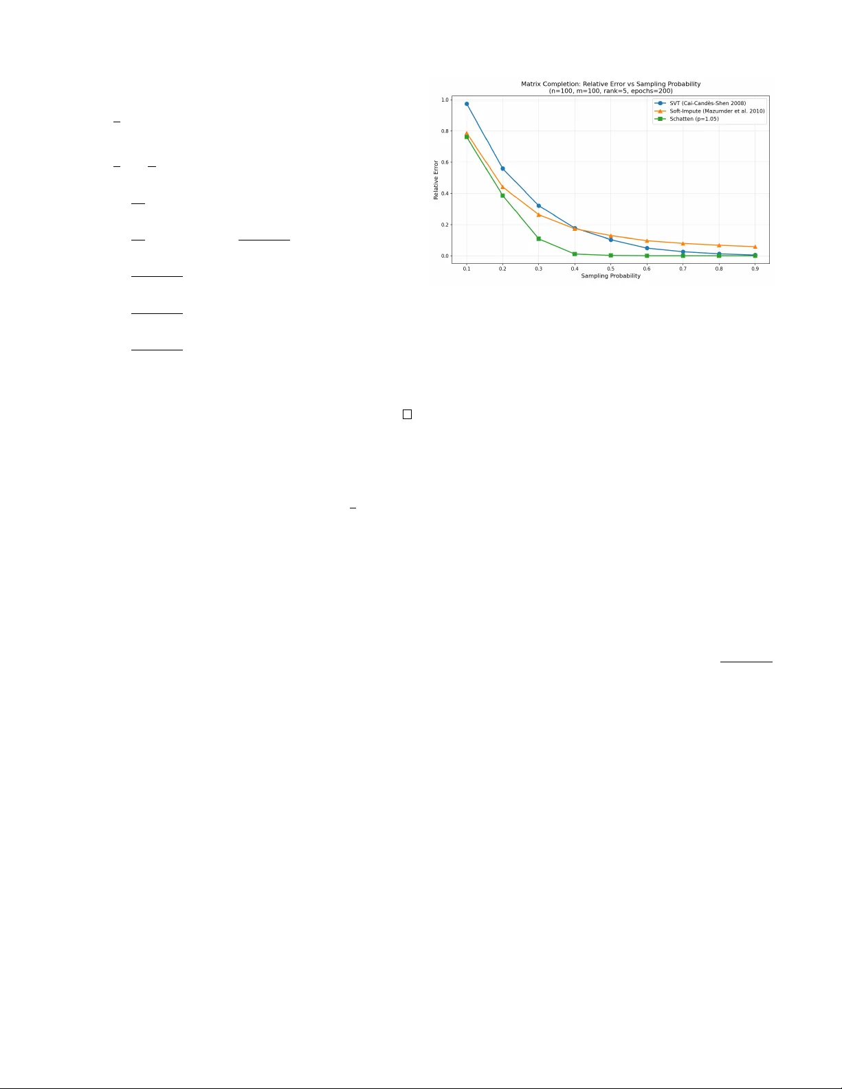
Implicit Bias and Con v er gence of Matrix Stochastic Mirror Descent Danil Akhtiamov ∗ Computing+Mathematical Sciences Caltech Pasadena, CA dakhtiam@caltech.edu Reza Ghane ∗ Electrical Engineering Caltech Pasadena, CA rghanekh@caltech.edu Omead Pooladzandi Electrical Engineering Caltech Pasadena, CA omead@caltech.edu Babak Hassibi Electrical Engineering Caltech Pasadena, CA hassibi@caltech.edu Abstract —W e in vestigate Stochastic Mirror Descent (SMD) with matrix parameters and vector -valued predictions, a frame- work rele vant to multi-class classification and matrix completion problems. Focusing on the overparameterized regime, where the total number of parameters exceeds the number of training samples, we pr ove that SMD with matrix mirror functions ψ ( · ) con verges exponentially to a global interpolator . Furthermore, we generalize classical implicit bias results of vector SMD by demonstrating that the matrix SMD algorithm conv erges to the unique solution minimizing the Bregman diver gence induced by ψ ( · ) from initialization subject to interpolating the data. These findings rev eal how matrix mirror maps dictate inductive bias in high-dimensional, multi-output problems. Index T erms —Stochastic Mirror Descent, Con vergence, Im- plicit Bias, Nuclear Norm, Matrix Completion, Data Imputation I . I N T RO D U C T I O N The choice of optimization algorithm plays a crucial role in determining not only con vergence speed but also the properties of learned models in ov erparameterized machine learning. While gradient descent and its variants have become the main workhorse in large-scale optimization, recent theoret- ical insights rev eal that the geometry induced by different optimizers leads to fundamentally different solutions. This phenomenon, kno wn as implicit bias, has sparked rene wed interest in understanding ho w algorithmic choices shape the learning process beyond mere con vergence guarantees. Stochastic mirror descent (SMD) generalizes standard gra- dient descent by performing updates in a dual space induced by a mirror map ∇ ψ , where ψ : R p → R is a strongly con vex potential function. Specifically , for a giv en training loss L t ( w t ) computed with respect to the batch sampled at the time step t , step size η , and parameters w t ∈ R p at iteration t , SMD performs the following update: ∇ ψ ( w t +1 ) = ∇ ψ ( w t ) − η ∇ w L t ( w t ) (1) Setting ψ ( · ) = 1 2 ∥ · ∥ 2 2 recov ers standard SGD. The po wer of this framew ork lies in its flexibility: different potential functions ψ encode dif ferent geometries into the optimization dynamics. For overparameterized problems where multiple so- lutions interpolate the training data perfectly , SMD exhibits an implicit bias property - it conv erges to the solution minimizing * Equal contribution the Bre gman div ergence D ψ ( w , w 0 ) to the initialization w 0 among all global minimizers, where D ψ ( w , w 0 ) = ψ ( w ) − ψ ( w 0 ) − ∇ ψ ( w 0 ) T ( w − w 0 ) In particular , when initialized near zero w 0 ≈ 0 , SMD con verges to the interpolator minimizing ψ ( w ) among all in- terpolating solutions. This implicit bias pr operty of stochastic mirror descent implies that SGD finds the minimal ℓ 2 -norm solution among interpolators. V arious works ha ve established con ver gence and implicit bias for linear models with vector parameters and scalar labels, capturing the linear re gression and linear classification tasks [1]–[7]. In particular , [1] characterized the implicit bias of vector mirror descent, while [2] prov ed the con vergence of vector Stochastic Mirror Descent (SMD). More recently , [3] established an exponential con vergence rate for this setting. Furthermore, [5] extended the analysis of [6] and [7] regarding classification margins from gradient descent to the mirror descent framework. Howe ver , these works treat parameters as unstructured v ectors, potentially missing geometric properties encoded in their matrix representation. W e therefore extend this framework to matrix weights and v ector outputs, moti- vated by the observation that a plethora of problems in modern signal processing and data science, such as the matrix comple- tion problem, are naturally formulated as problems of finding matrices satisfying certain structural properties. Namely , we consider the following update rule for W t ∈ R d × k , which we refer to as Matrix SMD: ∇ ψ ( W t ) = ∇ ψ ( W t − 1 ) − η ∇ W L t ( W t − 1 ) After establishing conv ergence and implicit bias guarantees, we demonstrate a practical application of the matrix SMD. Using the mirror function ψ ( W ) = P m i =1 σ i ( W ) p , where σ i ( W ) denotes the i -th singular value of W , we fit a linear model to solv e the matrix completion problem. Setting p ≈ 1 to approximate the nuclear norm yields a low-rank solution, which is a standard hypothesis for the matrix completion task. W e demonstrate empirically that Matrix SMD leads to a lower error than standard singular value thresholding methods, which are usually used for minimizing the nuclear norm in practice. I I . N O TA T I O N A N D P RO B L E M F O R M U L A T I O N A. The pr oblem W e consider the problem of recovering a matrix W ∈ R d × k subject to linear constraints. Definition 1 (Linear Constraint System) . Let A : R d × k → R p be a linear operator with matrix repr esentation A = ( a 1 , . . . , a p ) T wher e each a i ∈ R d × k is treated as a vector . The constraint system is: A ( W ) = b equivalently A v ec ( W ) = b wher e b ∈ R p is a known vector . In the current exposition, we assume that d × k > p , a r e gime commonly referr ed to as the overparameterized re gime. Example 1 (Matrix Completion) . In matrix recovery , we observe a subset Ω = { ( i 1 , j 1 ) , . . . , ( i p , j p ) } ⊂ [ d ] × [ k ] of matrix entries. Her e: • p = | Ω | is the number of observed entries • A ( W ) q = W i q ,j q extr acts the ( i q , j q ) -th entry • b contains the observed values at positions Ω As this pr oblem is overparameterized (there is a linear space of valid solutions), we need additional hypotheses r egar ding W . A common assumption is that W is low-rank [8]. Example 2 (Multi-class Linear Classification) . Given n data points x 1 , . . . , x n ∈ R d with one-hot labels Y 1 , . . . , Y n ∈ R k : • Y i = e c ( i ) wher e c ( i ) ∈ [ k ] is the class of point i . • A ( W ) ij = x T i W ( j ) computes the pr ediction for class j . • The constraint A ( W ) = ( Y 1 , . . . , Y n ) ensur es perfect interpolation. B. Optimization F rame work W e propose to minimize the empirical risk with a novel algorithm, which we call Matrix Stochastic Mirror Descent, that can be described as follows: Definition 2 (T raining Objective) . The loss function takes the form: L ( W ) = 1 p p X i =1 ℓ i ( A ( W ) i − b i ) wher e each ℓ i : R → R + is a con vex loss function. Definition 3 (Matrix Stochastic Mirror Descent) . Given a str ongly con vex mirror potential ψ : R d × k → R , the SMD update rule is: ∇ ψ ( W t ) = ∇ ψ ( W t − 1 ) − η ∇ W L t ( W t − 1 ) wher e L t is the loss on a random batch sampled at iteration t : L t ( W ) = 1 B B X j =1 ℓ i j  A ( W ) i j − b i j  (2) C. Mathematical Pr eliminaries Before stating our main results, we remind the key defini- tions on con vexity: Definition 4 (Matrix Con vexity Properties) . A function f : R d × k → R is: 1) Con vex if f ( θ U + (1 − θ ) V ) ≤ θ f ( U ) + (1 − θ ) f ( V ) for all U , V and θ ∈ [0 , 1] 2) Strictly con vex if the inequality is strict for θ ∈ (0 , 1) 3) µ -strongly con vex if f ( V ) ≥ f ( U ) + T r ( ∇ f ( U ) T ( V − U )) + µ 2 ∥ U − V ∥ 2 F W e will also make extensi ve use of the following definition of Bregman Di vergence: Definition 5 (Matrix Bregman Di vergence) . F or a strictly con vex differ entiable mirr or function ψ : R d × k → R , the Br e gman divergence is: D ψ ( U , V ) = ψ ( U ) − ψ ( V ) − T r ( ∇ ψ ( V ) T ( U − V )) The Schatten p -norms will serv e as the main illustrating example of the matrix mirrors for us: Definition 6 (Schatten Norm) . The Sc hatten p -norm of W ∈ R d × k is: ∥ W ∥ Schatten ,p =   min( k,d ) X i =1 σ i ( W ) p   1 p wher e σ 1 ( W ) ≥ · · · ≥ σ min( k,d ) ( W ) ≥ 0 ar e the singular values. I I I . M A I N R E S U L T S A N D A P P L I C AT I O N S W e will require the following assumptions. Note that, contrary to most other works in the literature, we do not require the L -smoothness condition, thus relaxing the common assumptions ev en for the case of vector weights. Assumptions 1. 1) The mirr or ψ : R d × k → R is differ en- tiable and ν -str ongly con vex for a ν > 0 . 2) The training loss is of the form L ( W ) = 1 p p X i =1 ℓ i ( A ( W ) i − b i ) Mor eover , ℓ i is non-negative , has minimum ℓ i (0) = 0 , has a derivative ℓ ′ i which is continuous at 0 and is µ - strictly con vex for a µ > 0 . 3) The batc hes chosen for (2) ar e chosen in such a way that E L t = L , where the expectation is taken with r espect to the randomness in the c hoice of the batch. 4) η > 0 is small enough, so that ψ − η L t is con vex. 5) The matrix A =  a 1 , a 2 , . . . , a p  T ∈ R ( d × k ) × p satisfies σ p ( A ) > 0 . Note that, in particular , this implies that we ar e in the overpar ameterized r e gime, i.e. that p < dk . 6) Let W ∗ be the unique minimizer of the following opti- mization pr oblem: min W D ψ ( W , W 0 ) , s.t. A ( W ) = b (3) Denote B = { W : D ψ ( W ∗ , W ) ≤ D ψ ( W ∗ , W 0 ) } Then there exists a C > 0 , such that the following holds for all W ∈ B : ∥∇ 2 ψ ( W ) ∥ op ≤ C W e are now ready to state our main result characterizing the implicit bias and the con vergence rate of Matrix SMD: Theorem 1 (Con vergence Rate and the Implicit Bias) . Assume that the linear oper ator A : R d × k → R p , the mirr or ψ : R d × k → R and the training losses L t : R d × k → R satisfy assumptions 1-4 fr om the list of Assumptions 1, whose notation is also embr aced below . Intr oduce W ∗ ∈ R d × k as the unique minimizer of the following objective: min W D ψ ( W , W 0 ) , s.t. A ( W ) = b (4) Denote the t -th iteration of the SMD algorithm defined via (2) with mirr or ψ trained to minimize L ( W ) and initialized at W 0 by W t . Then W t con verges to W ∗ as t → ∞ . Assume, in addition, that assumption 5 and 6 fr om the list of Assumptions 1 holds as well and let L := max U , V ∈B D ψ ( U , V ) ∥ U − V ∥ 2 F Then W t con verges to W ∗ exponentially , namely the follow- ing holds: E ∥ W ∗ − W t ∥ 2 F ≤ 2 ν  1 − η µσ p ( A ) 2 2 pL  t D ψ ( W ∗ , W 0 ) (5) Her e, the e xpectation is taken with r espect to the randomness in the batch c hoice at the step i for all i = 1 , . . . , t . Remark 1. T o ensure (5) implies exponential con verg ence, one must verify that the value of L is finite. This is true as B is compact and D ψ ( U , V ) ∥ U − V ∥ 2 F r emains bounded as U → V because of the assumption 6) fr om the list of Assumptions 1. Remark 2. Assumption 5 always holds for the matrix com- pletion problem from Example 1. F or the multi-class linear classification fr om Example 2, we have A = X ⊗ I k and assumption 5 holds if and only if σ n ( X ) > 0 . Example 3. ψ ( W ) = ∥ W ∥ p Schatten ,p + ν ∥ W ∥ 2 F satisfies all of the Assumptions 1 if p ≥ 2 . Hence, we can deduce exponential con vergence in this case. Example 4. As for 2 > p > 1 , ψ ( W ) = ∥ W ∥ p Schatten ,p + ν ∥ W ∥ 2 F satisfies assumptions 1-5 fr om the list of the Assump- tions 1. It also satisfies assumption 6 if and only if B does not contain singular matrices. Thus, in gener al, we can deduce con vergence for 2 > p > 1 but cannot specify the rate . I V . P R O O F S A. Pr oof of Con ver gence The following lemma is a matrix analog of Lemma 4.1 from [9]: Lemma 1. F or any S , U , V ∈ R d × k and any f : R d × k → R , the following identity holds: D f ( V , S ) + D f ( S , U ) − D f ( V , U ) = T r  ( ∇ f ( U ) − ∇ f ( S )) T ( V − S )  Pr oof. The proof is identical to the proof of Lemma 4.1 from [9]. Lemma 2. The following identity holds for any W satisfying A ( W ) = b , wher e W i denote the iterates of the SMD algorithm, stochastic loss functions L i : R d × k → R and a learning rate η > 0 satisfying Assumptions 1. D ψ ( W , W i − 1 ) = η D L i ( W , W i − 1 )+ D ψ ( W , W i ) + D ψ − η L i ( W i , W i − 1 ) + η L i ( W i ) Pr oof. T ake an arbitrary W ∈ R d × k . Using Lemma 1: D ψ ( W , W i ) + D ψ ( W i , W i − 1 ) − D ψ ( W , W i − 1 ) = T r  ( ∇ ψ ( W i − 1 ) − ∇ ψ ( W i )) T ( W − W i )  Incorporating the definition of the SMD update, we arriv e at: D ψ ( W , W i ) + D ψ ( W i , W i − 1 ) − D ψ ( W , W i − 1 ) (6) = η T r  ( ∇L i ( W i − 1 )) T ( W − W i )  (7) W e also have from Lemma 1 applied to f = L i : η D L i ( W , W i ) + η D L i ( W i , W i − 1 ) − η D L i ( W , W i − 1 ) = η T r  ( ∇L i ( W i − 1 ) − ∇L i ( W i )) T ( W − W i )  (8) Subtracting (8) from (6) we obtain: D ψ − η L i ( W , W i ) + D ψ − η L i ( W i , W i − 1 ) − D ψ − η L i ( W , W i − 1 ) = η T r  ∇L i ( W i )) T ( W − W i )  (9) Equation (9) is equiv alent to: D ψ ( W , W i − 1 ) = η D L i ( W , W i − 1 ) + D ψ − η L i ( W , W i ) + D ψ − η L i ( W i , W i − 1 ) − η T r  ∇L i ( W i )) T ( W − W i )  Opening up the D ψ − η L i ( W , W i ) term further: D ψ ( W , W i − 1 ) = η D L i ( W , W i − 1 ) + D ψ ( W , W i ) − η D L i ( W , W i ) + D ψ − η L i ( W i , W i − 1 ) − η T r  ∇L i ( W i )) T ( W − W i )  Grouping the terms having η in front: D ψ ( W , W i − 1 ) = η D L i ( W , W i − 1 ) + D ψ ( W , W i ) + D ψ − η L i ( W i , W i − 1 ) − η  D L i ( W , W i ) + T r  ∇L i ( W i )) T ( W − W i )  By definition of D L i ( W , W i ) we arriv e at: D ψ ( W , W i − 1 ) = η D L i ( W , W i − 1 ) + D ψ ( W , W i ) + D ψ − η L i ( W i , W i − 1 ) − η ( L i ( W ) − L i ( W i )) W e are now prepared to sho w con vergence: Pr oof. Assuming W interpolates all data, i.e. L i ( W ) = 0 for all i , we obtain the matrix analog of Lemma 6 from [5] for any W from the interpolating manifold: D ψ ( W , W i − 1 ) = η D L i ( W , W i − 1 ) + D ψ ( W , W i ) + D ψ − η L i ( W i , W i − 1 ) + η L i ( W i ) W e are ready to prove con ver gence no w . Note that Lemma 2 implies that D ψ ( W , W t − 1 ) ≥ D ψ ( W , W t ) + η L i ( W i ) for all i = 1 , . . . , T . Summing over i = 1 , . . . , T , we hav e: T X i =1 D ψ ( W , W t − 1 ) ≥ T X i =1 D ψ ( W , W t ) + η T X i =1 L i ( W i ) Hence, D ψ ( W , W 0 ) ≥ D ψ ( W , W T ) + η T X i =1 L i ( W i ) Therefore, we see that L T ( W T ) → 0 as T → ∞ , implying that A ( W T ) → b as T → ∞ and thus all SMD updates ∇L T ( W T ) → 0 as well, implying con ver gence to some point W ∞ . B. Implicit Bias Summing up the SMD iterations, we note that ∇ ψ ( W t ) − ∇ ψ ( W 0 ) = t X s =1 η ∇L s ( W s ) Consider the follo wing optimization problem, whose solution W is unique due to strong conv exity: min W ∈ R d × k D ψ ( W , W 0 ) s.t A ( W ) = b Using a Lagrange multiplier λ ∈ R p : min W ∈ R d × k max λ ∈ R p D ψ ( W , W 0 ) + λ T ( A ( W ) − b ) W e compute the stationary conditions of KKT (the solution to this is unique as well): ( ∇ ψ ( W ) − ∇ ψ ( W 0 ) = A T λ A ( W ) = b (10) where A is the matrix representation of A such that A ( W ) = A vec ( W ) . Now considering L s ( W ) := 1 B B X ij =1 ℓ i j  A ( W ) i j − b i j  , we hav e for the SMD iterations: ∇ ψ ( W t ) − ∇ ψ ( W 0 ) = η t X s =1 ∇L s ( W s ) = η t X s =1 1 B B X j =1 ℓ ′ i j  A ( W s ) i j − b i j  ∇A ( W ) i j = A T µ t for some µ t ∈ R p because ev ery ∇A ( W ) i j belongs in the span of a 1 , . . . , a p . Now , assume that the SMD with constant step-size con- ver ges to some point W ∞ ∈ R d × k . This implies that ∇L ( W ∞ ) = 0 , which by assumption implies A ( W ∞ ) = b . W e also observe that ∇ ψ ( W t ) − ∇ ψ ( W 0 ) = A T µ t for all t ∈ N . Thus, taking λ := µ ∞ , we observe that W ∞ satisfies the KKT conditions (10), which are assumed to yield a unique solution W ∗ . C. Con ver gence Rate The proof below was inspired by the proofs provided in [3] and [10]. Lemma 3. The following holds: D ψ ( W ∗ , W t − 1 ) ≥ η D L t ( W ∗ , W t − 1 ) + D ψ ( W ∗ , W t ) Pr oof. F ollows from D ψ ( W , W i − 1 ) = η D L i ( W , W i − 1 ) + D ψ ( W , W i ) + D ψ − η L i ( W i , W i − 1 ) + η L i ( W i ) Lemma 4. Let W ∗ − W t − 1 = P + P ⊥ , wher e vec ( P ) ∈ range ( A T ) and A vec ( P ⊥ ) = 0 . Then A ( W t − 1 + P ) = b Pr oof. Since A ( W ∗ ) = b and A vec ( P ⊥ ) = 0 by definition, we hav e A ( W t − 1 + P ) = A ( W ∗ − P ⊥ ) = b Lemma 5. The following holds:  1 − η µσ p ( A ) 2 2 pL  E D ψ ( W ∗ , W t − 1 ) ≥ E D ψ ( W ∗ , W t ) Pr oof. It suf fices to sho w the following due to Lemma 3: η E D L t ( W ∗ , W t − 1 ) ≥ η µσ p ( A ) 2 2 pL D ψ ( W ∗ , W t − 1 ) Since the e xpectation is taken ov er the randomness in the SMD batch, the latter is equiv alent to: D L ( W ∗ , W t − 1 ) ≥ µσ p ( A ) 2 2 pL D ψ ( W ∗ , W t − 1 ) By strong con vexity of ℓ i , D L ( W ∗ , W t − 1 ) = 1 p p X i =1 D ℓ i ( A ( W ∗ ) i − b i , A ( W t − 1 ) i − b i ) ≥ 1 p p X i =1 µ 2 ( A ( W ∗ ) i − A ( W t − 1 ) i ) 2 = µ 2 p ∥A ( W ∗ ) − A ( W t − 1 ) ∥ 2 2 = µ 2 p ∥ A vec ( P ) ∥ 2 2 ≥ µσ p ( A ) 2 2 p ∥ P ∥ 2 F = µσ p ( A ) 2 2 p ∥ P + W t − 1 − W t − 1 ∥ 2 F ≥ µσ p ( A ) 2 2 pL D ψ ( P + W t − 1 , W t − 1 ) ≥ µσ p ( A ) 2 2 pL D ψ ( W ∗ , W t − 1 ) Note that in the last line abo ve we used that A ( P + W t − 1 ) = b and that W ∗ minimizes D ψ ( W , W t − 1 ) with respect to the constraint A ( W ) = b . V . E X P E R I M E N TA L S E T U P W e consider the problem of recovering a low-rank matrix M ∈ R n × m from a subset of its entries. The true matrix is generated as M = UV T where U ∈ R n × r and V ∈ R m × r hav e i.i.d. Gaussian entries scaled by 1 / √ r , ensuring rank r . W e observe each entry independently with probability pr ob , yielding the observation set Ω and the partially observed matrix M Ω . Since the common assumption regarding M is lo w- rankness, approaches to the matrix completion problem usually solve the follo wing objective: min W ∥ W ∥ ∗ (11) s.t. W ij = M ij , ( i, j ) ∈ Ω where ∥ · ∥ ∗ denotes the nuclear norm (sum of singular values). A. Methods W e compare three algorithms for low-rank matrix comple- tion driv en by singular value shrinkage. Definition 7 (Singular V alue Soft-Thresholding) . F or a matrix with singular value decomposition W = U diag ( σ ) V T the soft-thr esholding operator S τ is defined as: S τ ( W ) = U · diag (max( σ i − τ , 0)) · V T wher e τ > 0 is the thr eshold parameter . 1. Singular V alue Thresholding (SVT) [11] maintains an auxiliary matrix Y t and iterates W t = S τ ( Y t − 1 ) (12) Y t = Y t − 1 + δ P Ω ( M − W t ) , (13) where P Ω is the projection onto observ ed entries, i.e. P Ω keeps the values for the entries in Ω and sets the rest to zero. Fig. 1. Relative recov ery error versus sampling probability for SVT [11], Soft-Impute [12], and Schatten- p SMD. 2. Soft-Impute [12] iterates as ( Z t ) ij = ( M ij if ( i, j ) ∈ Ω ( W t ) ij otherwise (14) W t +1 = S λ ( Z t ) , (15) 3. Schatten- p Mirror Descent: Our proposed method using the mirror ψ ( W ) = ∥ W ∥ p Schatten ,p with p slightly above 1 (we use p = 1 . 05 ). B. Results W e e valuate all methods on 100 × 100 matrices of rank 5 , varying the sampling probability from 0 . 1 to 0 . 9 in increments of 0 . 1 . Each method runs for 200 iterations. For the SVT method we use step size δ = 0 . 8 ; the SVT shrinkage parameter is set to the paper-style default τ = 5 max( n, m ) . For Soft-Impute we use λ = 1 . 0 . For Schatten- p SMD we use p = 1 . 05 and learning rate η = 50 , with the gradient normalized by | Ω | . Figure 1 shows the relativ e Frobenius norm error ∥ W − M ∥ F ∥ M ∥ F as a function of sampling probability . The Schatten- p mirror descent consistently outperforms both thresholding methods across all sampling rates, with the advantage most pronounced at lower sampling probabilities where the problem is most challenging. V I . C O N C L U S I O N This paper extends the theory of stochastic mirror descent to matrix parameters and vector -valued outputs, providing both theoretical guarantees and practical benefits. Our experiments on matrix completion validate the practical value of this framew ork. Schatten- p mirror descent with p ≈ 1 outperforms standard proximal methods based on singular value thresholding ran with the same number of epochs, particularly in challenging lo w-sampling regimes, by naturally inducing lo w-rank structure through the geometry of the mirror map rather than explicit constraints. While our analysis establishes conv ergence for SMD with 1 < p < 2 , proving exponential rates in this regime requires relaxing assumption 6 in the list of Assumptions 1. This remains an important direction for future work. R E F E R E N C E S [1] S. Gunasekar , J. Lee, D. Soudry , and N. Srebro, “Characterizing implicit bias in terms of optimization geometry , ” in International Conference on Machine Learning . PMLR, 2018, pp. 1832–1841. [2] N. Azizan and B. Hassibi, “Stochastic gradient/mirror descent: Minimax optimality and implicit regularization, ” arXiv pr eprint arXiv:1806.00952 , 2018. [3] K. N. V arma and B. Hassibi, “Exponential con vergence of stochastic mirror descent in over -parameterized linear models, ” in ICASSP 2025 - 2025 IEEE International Conference on Acoustics, Speech and Signal Pr ocessing (ICASSP) , 2025, pp. 1–5. [4] H. Sun, K. Ahn, C. Thrampoulidis, and N. Azizan, “Mirror descent maximizes generalized margin and can be implemented efficiently , ” Ad- vances in Neural Information Processing Systems , vol. 35, pp. 31 089– 31 101, 2022. [5] N. Azizan, S. Lale, and B. Hassibi, “Stochastic mirror descent on overparameterized nonlinear models, ” IEEE Tr ansactions on Neural Networks and Learning Systems , vol. 33, no. 12, pp. 7717–7727, 2021. [6] D. Soudry , E. Hoffer , M. S. Nacson, S. Gunasekar, and N. Srebro, “The implicit bias of gradient descent on separable data, ” Journal of Machine Learning Resear ch , vol. 19, no. 70, pp. 1–57, 2018. [7] Z. Ji and M. T elgarsky , “The implicit bias of gradient descent on nonseparable data, ” in Confer ence on learning theory . PMLR, 2019, pp. 1772–1798. [8] B. Recht, M. Fazel, and P . A. Parrilo, “Guaranteed minimum-rank solutions of linear matrix equations via nuclear norm minimization, ” SIAM r eview , vol. 52, no. 3, pp. 471–501, 2010. [9] A. Beck and M. T eboulle, “Mirror descent and nonlinear projected subgradient methods for con vex optimization, ” Operations Research Letters , vol. 31, no. 3, pp. 167–175, 2003. [10] R. D’Orazio, N. Loizou, I. H. Laradji, and I. Mitliagkas, “Stochastic mirror descent: Conv ergence analysis and adaptive variants via the mirror stochastic polyak stepsize, ” Tr ans. Mach. Learn. Res. , 2023. [11] J.-F . Cai, E. J. Cand ` es, and Z. Shen, “ A singular value thresholding al- gorithm for matrix completion, ” SIAM Journal on optimization , vol. 20, no. 4, pp. 1956–1982, 2010. [12] R. Mazumder, T . Hastie, and R. Tibshirani, “Spectral regularization algorithms for learning large incomplete matrices, ” The Journal of Machine Learning Research , vol. 11, pp. 2287–2322, 2010.