A Dataset is Worth 1 MB

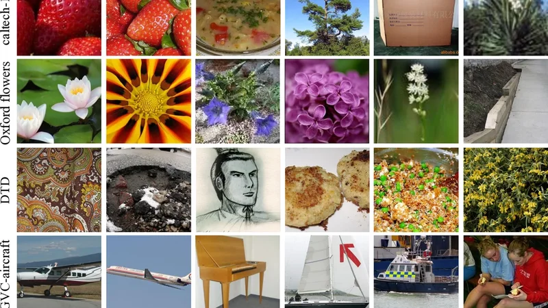
A Dataset is W orth 1 MB Elad Kimchi Shoshani 1 Leeyam Gabay 1 Y edid Hoshen 1 Abstract A dataset server must often distrib ute the same large payload to man y clients, incurring massi ve communication costs. Since clients frequently operate on di verse hardware and softw are frame- works, transmitting a pre-trained model is of- ten infeasible; instead, agents require raw data to train their own task-specific models locally . While dataset distillation attempts to compress training signals, current methods struggle to scale to high-resolution data and rarely achieve suf- ficiently small files. In this paper , we propose Pseudo-Labels as Data (PLAD A), a method that completely eliminates pixel transmission. W e as- sume agents are preloaded with a large, generic, unlabeled refer ence dataset (e.g., ImageNet-1K, ImageNet-21K) and communicate a ne w task by transmitting only the class labels for specific im- ages. T o address the distribution mismatch be- tween the reference and target datasets, we in- troduce a pruning mechanism that filters the ref- erence dataset to retain only the labels of the most semantically rele vant images for the tar get task. This selection process simultaneously maxi- mizes training efficienc y and minimizes transmis- sion payload. Experiments on 10 div erse datasets demonstrate that our approach can transfer task kno wledge with a payload of less than 1 MB while retaining high classification accurac y , offering a promising solution for efficient dataset serving. 1. Introduction Sending training datasets from a central server to multi- ple clients is an expensi ve process, as large datasets must be transmitted repeatedly . This places a heavy burden on dataset servers. Reducing this communication cost is there- fore critical. Crucially , sending pre-trained model weights instead of datasets is often insufficient. In many practi- 1 School of Computer Science and Engineering, The Hebrew Univ ersity of Jerusalem, Israel. Correspondence to: Elad Kimchi Shoshani < elad.shoshani@mail.huji.ac.il > . Pr eprint. F ebruary 27, 2026. cal scenarios, clients are heterogeneous—ranging from di- verse autonomous v ehicles to medical devices—and must train models using specific software framew orks (e.g., Py- T orch, J AX) or bespoke hardware. Consequently , the server must transmit the training data to allo w agents to optimize their own unique models locally . A secondary challenge arises in scenarios where the communication channel is sev erely bandwidth-constrained. Examples include under- water acoustic links to deep-sea vehicles (up to ∼ 5 kbps) ( LinkQuest Inc. , 2007 ; W on & Park , 2012 ; Annalakshmi et al. , 2017 ) or the T itan rover where direct-to-Earth links can be on the order of ∼ 500–800 bps ( Abelson , 2005 ; Ole- son et al. , 2015 ). In such cases, transmitting a typical mid- sized (1 GB) dataset would take days to months and can be ener getically prohibiti ve. Addressing these scenarios requires methods capable of compressing training datasets by orders of magnitude while minimizing accuracy loss. A prominent line of research addressing this challenge is dataset distillation. This approach aims to replace a large training dataset with a compact set of synthetic images and labels, such that a model trained on them minimizes re- gret with respect to the original data. Despite its promise, synthesizing these learning-efficient images is computation- ally and numerically challenging. While easier on smaller benchmarks like CIF AR-10 ( Krizhevsky , 2009 ), scaling these methods to high-resolution datasets is difficult. The core challenge lies in unrolling optimization steps ( Cui et al. , 2023 ) due to high memory requirements and unstable in- ner loop optimization. Furthermore, the continuous, full- precision nature of these synthetic pixels often results in file sizes that remain prohibiti vely large. Finally , dataset distillation struggles with mismatched server and client ar- chitectures, although there has been progress on this front. In this paper , we inv ert the standard framework of dataset distillation. Rather than synthesizing images while keeping the labels fixed, we synthesize labels while keeping the im- ages fixed. W e assume each remote agent is preloaded with a standardized, large, unlabeled set of images, which we term the r efer ence dataset. T o communicate a new task, we do not transmit pixels; instead, we provide only the class la- bels for specific images within this reference dataset. Since a label is merely a compact inte ger index, the transmission payload is drastically reduced. The agent then utilizes its stored reference images and the newly receiv ed labels to 1 A Dataset is W orth 1 MB F igur e 1. Motivation. A dataset server transmits the same large dataset many times at massi ve cost. Our method allo ws the server to send a compressed payload of less than 1 MB, enabling clients with heterogeneous hardware, ev en if they have ultra-narro w band- width, to train their own models locally . locally train the target model. In essence, we replace expen- siv e pixel transmission with on-device storage and highly compressed labels. This approach faces two immediate hurdles: distribution mismatch and ef ficiency . First, the majority of images in a generic reference dataset are likely semantically unrelated to the target task and can hurt learning. Second, for large reference datasets with many classes, transmitting a label for e very image remains bandwidth-intensi v e. W e propose a unified solution to both problems: dataset pruning. W e select only a small fraction of reference images for training, ignoring the rest. This ensures that only images semantically related to the target task are used, while simultaneously reducing the transmission cost, as indicating that an image should be ignored requires only a single bit. T o achie v e this, we introduce a pruning heuristic inspired by out-of- distribution (OOD) detection. W e validate our frame work on 10 di verse natural-image datasets and 4 medical (OOD) datasets, utilizing unlabeled ImageNet-1K ( Deng et al. , 2009 ) and ImageNet-21K ( Rid- nik et al. , 2021 ) as reference datasets. W e demonstrate the ability to transmit the information required to learn a novel task in less than 1 MB, often with only small loss in ac- curacy . W e even find non-tri vial accuracy when the tar get datasets are medical and distrib utionally distant from the reference set. Qualitativ e analysis confirms that our selec- tion procedure successfully identifies semantically rele vant images, validating the method’ s effecti veness. Furthermore, we analyze the trade-of fs between reference dataset size and transmission payload, and provide ablations on different coding schemes. Our contributions are as follo ws: 1. W e propose a new method: Pseudo-Labels as Data , which transmits only hard labels while achie ving high performance, reducing the transfer payload to a well below one bit per reference image (e.g., 85–206KB at 1% keep on ImageNet-21K after Zstd; T able 4 ). 2. W e introduce an effecti ve pruning mechanism using Energy-based OOD scores. W e show that filtering the reference dataset to just 1%-10% of images both improv es accuracy and reduces bandwidth costs. 3. W e demonstrate that our method achieves high accu- racy on di v erse classification tasks while transmitting a payload of less than 1 MB. 2. Related W orks Dataset and Label Distillation. Dataset distillation (a.k.a. dataset condensation) compresses a full training set into a tiny synthetic set such that training on it approximates training on the original data ( W ang et al. , 2018 ; Y u et al. , 2023 ). While effecti ve on smaller benchmarks, scaling these methods to high-resolution repositories like ImageNet-21K has historically been limited by exorbitant compute/memory consumption during optimization ( Zhao et al. , 2021 ; Cui et al. , 2023 ; Cazena vette et al. , 2022 ; Du et al. , 2023 ). Re- cent work suggests that the labels can be the primary dri ver of successful distillation—motiv ating approaches that learn or distill labels rather than synthesizing pixels ( Sucholutsky & Schonlau , 2021 ; Ondrej Bohdal , 2020 ; Qin et al. , 2024 ). PLAD A takes this perspectiv e to the extreme: instead of transmitting images, we communicate a task by transmitting only hard pseudo-labels for a fixed, preloaded reference image set. Knowledge Distillation and Pseudo Labels. Kno wledge distillation trains a student model to match the predictions of a teacher , typically using soft targets/logits to transfer knowledge across architectures ( Hinton et al. , 2015 ; Nayak et al. , 2019 ; W ang & Y oon , 2021 ; Mansourian et al. , 2025 ). When original training data is unav ailable, data-free dis- tillation synthesizes inputs ( Nayak et al. , 2019 ) or recon- structs them from a trained model ( Y in et al. , 2020 ); re- cent work also frames distillation as an efficient mechanism for faster con ver gence and improved transfer ( He et al. , 2022 ). Pseudo-labeling and self-training treat a model’ s high-confidence predictions as supervision, often paired with confidence filtering and meta-learning to improv e label quality ( Lee , 2013 ; Sohn et al. , 2020 ; Xie et al. , 2020 ; Pham et al. , 2021 ; Kage et al. , 2024 ). PLADA turns this idea into a communication primitiv e: a server -side teacher generates hard pseudo-labels on a shared reference dataset, and clients train locally using these pseudo-labels as data . OOD Detection and Data Pruning/Selection. Deep net- works are often ov erconfident under distribution shift, moti- vating out-of-distribution (OOD) detection methods based on softmax confidence ( Hendrycks & Gimpel , 2017 ), tem- 2 A Dataset is W orth 1 MB T rai n Ps eu d o - L ab el Base Serve r T ar g et Data set T ea cher Log it Gen eration Filter ing (Ene r gy + S a fe ty - N e t) Co m p re ss (I ndice s + L a be ls)     IN - 21K R e f. S e t (S e rv e r) IN - 21 K Student      Recon struct (Se lec t by I nde x )   F il tere d R e f. S e t R e f. S e t (Lo c a l) Remote Clie nt P a y lo a d < 1 MB T rai n F igur e 2. The PLAD A Pipeline. The server (left) trains a teacher classifier on the task dataset and distills this task knowledge into hard labels on the reference data. It then filters to the lowest-uncertainty p % of pseudo-labels and transmits a compressed payload ( < 1 MB). The client (right) reconstructs a virtual dataset using its preloaded reference dataset and the payload to train the student model. perature/perturbation scoring (ODIN) ( Liang et al. , 2018 ), feature-density scores such as Mahalanobis distance ( Lee et al. , 2018 ), and energy-based criteria ( Liu et al. , 2020 ). T raining-time modifications can also improve confidence separation (e.g., LogitNorm) ( W ei et al. , 2022 ; Ding et al. , 2025 ), and recent work further improves distance-based OOD scoring by dynamically calibrating geometry at test time ( Guo et al. , 2025 ). Closely related are data selection and pruning methods that reduce training cost while pre- serving accuracy ( Sorscher et al. , 2022 ; Y ang et al. , 2023b ), including approaches that explicitly combine pruning with knowledge distillation to mitigate accuracy loss at high prun- ing rates ( Ben-Baruch et al. , 2024 ). PLAD A ’ s pruning stage lev erages uncertainty/OOD scores to select semantically rel- ev ant reference examples before label transmission, aligning with this literature while operating in a communication- limited dataset-serving setting. 3. Problem F ormulation In our setting, there is a central server (denoted A s ) and multiple remote agents (denoted A r ). W e preload all remote agents with the same reference dataset D r containing n unlabeled samples D r = { x 1 , x 2 , . . . , x n } drawn from a distribution D r . After deployment, when the remote agents are distant from the central server , a new target task arises with distribution D t . Each sample consists of a pair ( x, y ) , where the input is x and the tar get label is y . In this paper , we assume the tar get label is discrete, making the task a classification problem; we leav e the extension to regression for future work. Our objectiv e is to train a classifier f on the remote agent that achie ves high accuracy in predicting y giv en x for ( x, y ) ∼ D t . T o fulfill this task, the server A s transmits a payload P of size b bytes to each remote agent A r . W e assume the remote agent is capable of training a model gi ven input data. The objectiv e is to maximize the accuracy of classifier f while satisfying the constraint that the transmitted payload does not exceed b bytes. 4. Method 4.1. Overview Our core approach is illustrated in Figure 2 . The central server first trains a ground-truth classifier , f g t , on the train- ing data from the target distribution D t . It utilizes this classifier to generate pseudo-labels for the reference dataset. The server then transmits these pseudo-labels as the pay- load to the remote agent. Finally , the remote agent trains a student classifier f on the reference set using the receiv ed labels. In Section 4.3 , we present pruning methods to sig- nificantly reduce the number of class labels transmitted. In Section 4.4 , we describe variable-length coding methods that lev erage the statistical properties of the labels to further compress the payload size. 4.2. Efficient Classifier T ransfer via Hard Pseudo-Labels T ransmitting a full dataset to a remote agent requires band- width that often exceeds 1 GB. While subsampling datasets (e.g., via coreset selection) can reduce size by 50-80%, it typically incurs a significant penalty in accuracy . For ex- treme bandwidth constraints, this reduction is insufficient. Dataset distillation aims to create synthetic images with aggressiv e compression; ho we ver , these methods often re- sult in accuracy loss and still require payloads measuring in megabytes. Our core premise is that for classification tasks, labels con- tain far more information per byte than images. Howe ver , labels must be associated with images, which are expensiv e to transmit. T o resolve this, we utilize a fixed reference dataset preloaded on each remote agent. T o transmit a tar get task, we send only the pseudo-labels corresponding to the images in this reference dataset. W e utilize hard labels rather than soft labels, as storing soft labels requires significantly 3 A Dataset is W orth 1 MB more memory . Label generation. Since the reference dataset is generic, many of its images may not correspond to any classes in the target task. W e propose a two-step procedure. First, we train a classifier f g t on the training data from the tar get distribution D t : f g t ← arg min f 1 n targ et X ( x,y ) ∼D t L C E ( f ( x ) , y ) (1) W e then label each image in the reference set using the classifier f g t , assigning each image the label corresponding to the maximal logit: l i = arg max q f g t ( x i )[ q ] (2) The server sends a payload consisting of the hard labels for the reference set images: P = [ l 1 , l 2 , . . . , l n ] (3) Let k denote the number of target classes. Naiv ely sending the reference set labels requires n log 2 k bits. After trans- mission, the agent trains a classifier based on the locally stored reference images and the receiv ed labels: f ← arg min f ′ 1 n n X i =1 L C E ( f ′ ( x i ) , l i ) (4) The resulting classifier f on the client serves as the final student model. 4.3. Reference Dataset Pruning T ransmitting a label for ev ery reference image is suboptimal. First, it hurts accuracy: some reference images do not fit any target task classes. For example, an image yielding roughly equal logits for all classes is lik ely a poor repre- sentativ e for an y of them. Forcing such an image into a hard class introduces noise that degrades the target training process. Second, sending a label requires log 2 k bits per image, which becomes expensi ve for large reference sets. Ideally , we should transmit only informativ e labels. Selecting inf ormative images. W e draw inspiration from semi-supervised learning, which applies a predictor to a large set of potentially irrele vant images. T o isolate relev ant samples, these approaches use distribution measures to filter for images where the label certainty is high. Concretely , we retain the top p % of images based on an uncertainty score (where lo wer is better). W e ev aluated se veral out-of- distribution metrics and found that Logit Energy achie v ed the best results, with Shannon Entropy performing compa- rably (see T able 7 ). W e compute energy as: E ( x ; f g t ) = − log k X j =1 exp( f g t ( x )[ j ]) (5) ca lt e ch - 1 0 1 DT D F GV C - air cr af t 0 . 1 % 0 . 5 % 1 0 % 5 0 % 0 . 0 0 0 1 % 1 . 5 % O x f or d f l ow e r s F igur e 3. Reference set images vs. energy percentile. High- confidence (lo w-energy) samples retrie ved from ImageNet-21K demonstrate semantic and structural alignment with the tar get domains. For additional visualizations see Appendix C . In a large reference dataset like ImageNet-21K, typically only a small fraction of images are relev ant to a specific downstream task. As shown in Figure 3 , images semanti- cally related to the target dataset often appear only within the top 1% of lowest ener gy scores. Overall, we find that pruning uncertain labels of fers three ad- vant ages: (i) lo wer transmission cost, (ii) increased accurac y for the client’ s target classifier , and (iii) reduced training time due to the smaller dataset size. See Section 5.2 for experimental results. Safety-Net Filtering. While energy-based pruning effec- tiv ely selects high-confidence samples, it suffers from a significant drawback in high-compression regimes: it dis- proportionately removes samples from “harder” or under- represented classes. When the global retention ratio is lo w (e.g., 1%), the filtered dataset is ofte n dominated by a fe w “easy” classes, leading to class collapse and poor student generalization. Figure 4 illustrates this issue. T o mitigate this, we propose a Safety-Net filtering mecha- nism. Instead of relying solely on a global energy threshold, we reserve a portion s of the bandwidth budget to ensure that all classes are preserv ed. W e define a class-specific quota K c for each class c based on a po wer-la w weighting of its original size N c : K c ∝ ( N c ) α (6) where α is a balancing h yperparameter . • α = 1 : proportional retention (preserves the original imbalance). • α = 0 : uniform retention (equal quota per class). 4 A Dataset is W orth 1 MB • α < 0 : tail-fav oring retention (weak classes receiv e larger quotas). W e specifically explore ne gati ve α values (e.g., α = − 0 . 2 ). This setting intentionally ov er-samples from smaller or “weaker” classes, pro viding a structural guarantee that tail classes are preserved in the distilled dataset. T o construct the final payload, we first fill the Safety-Net quota using the best av ailable samples (lowest energy) per class, and then utilize the remaining b udget according to global logit energy , regardless of class membership. 4.4. V ariable-Length Coding Payload transmission can be optimized with suitable com- pression. A naiv e scheme for a payload with n ref reference images and a keep rat e of p % in v olves sending: (i) one bit per image indicating whether the label was retained, and (ii) log 2 k bits for the hard label of each retained image. This results in b raw bits: b raw = n ref (1 + p log 2 k ) (7) For large reference datasets, this o verhead is significant. For example, using ImageNet-21K ( ≈ 14 . 2 million images) as the reference with a 5% keep rate and 64 classes (6 bits), the payload is approximately 2 MB, the majority of which (1.69 MB) is consumed by the pruning mask (1 bit per reference set image image). W e can mitigate the cost of the pruning mask using Run- Length Encoding (RLE). Instead of storing all bits, we store the distance between consecuti v e k ept indices. For lo w k eep rates ( p ≪ 1 ), this exploits sparsity effecti v ely , reducing the av erage cost per selected item significantly compared to a dense bitmap. Furthermore, we exploit the statistical distribution of classes. Instead of using a fixed log 2 k bits per label, we employ variable-length encoding so that frequent classes are as- signed shorter codes. Huffman coding is a classical method lev eraging this principle. W e illustrate the class distribution in Fig. 4 . While these classical concepts highlight the sources of re- dundancy , modern implementations offer superior perfor- mance. In our experiments, we utilize Zstd ( Collet , 2021 ; Meta Platforms , 2026 ), a modern state-of-the-art compres- sion library , to compress the final pseudo-label payloads. 5. Experiments In this section, we ev aluate the proposed PLAD A frame- work. W e assess its ability to transfer task knowledge under extreme bandwidth constraints, analyze its rob ustness to out-of-distribution (OOD) tasks, and v alidate the ef ficacy of the Safety-Net filtering mechanism. 0 5 10 15 20 25 30 35 40 Class Index 0 10,000 100,000 500,000 1,500,000 4,500,000 9,000,000 Count (Cube Root Scale) Global Distribution After 5% Balanced Per-Class Filtering F igur e 4. Class distribution of the RESISC45 pseudo hard- labels , before and after filtering using safety-net. The yellow bars show the original global distrib ution, which is hea vily imbalanced - RESISC45 has images extracted using Google Earth, out of which class 0 is airplane . Standard global filtering would eliminate some of the tail classes entirely . The blue bars demonstrate our Safety-Net Filtering (keeping 5%, α = − 0 . 2 ), which ef fectiv ely preserves a representation of under-represented classes ev en under extreme compression. Note that the Y -axis uses a cube-root scale to visually accommodate the large magnitude dif ferences between the ‘strong‘ and ‘weak‘ classes. 5.1. Experimental Setup Datasets and Benchmarks. W e e valuate our method on 14 div erse classification datasets, categorized by domain to test generalization across varying granularities: • Coarse-grained Objects: Caltech-101 ( Li et al. , 2022 ), CIF AR-10 ( Krizhevsk y , 2009 ), and Places365 ( Zhou et al. , 2017 ). • F ine-gr ained Classification: CUB-200-2011 ( W ah et al. , 2022 ), DTD (T extures) ( Cimpoi et al. , 2014 ), FGVC-Aircraft ( Maji et al. , 2013 ), Food-101 ( Bossard et al. , 2014 ), Oxford-Flo wers-102 ( Nilsback & Zisser- man , 2008 ), Oxford-IIIT Pet ( Parkhi et al. , 2012 ), and RESISC45 ( Cheng et al. , 2017 ). • Medical (OOD Str ess T est): T o test the limits of our ap- proach on data distributionally disjoint from ImageNet, we utilize BloodMNIST , DermaMNIST , RetinaMNIST , and NCT -CRC-HE-100K ( Y ang et al. , 2021 ; 2023a ; Ignatov & Mali venk o , 2024 ). Data Leakage V erification: W e rigorously verified (see App. A ) that there is zero or statistically negligible intersec- tion ( < 1% ) between the tar get test sets and the ImageNet reference datasets, ensuring that student performance is not a result of memorization. Baselines. W e compare PLAD A against three transmis- sion strategies: 5 A Dataset is W orth 1 MB T able 1. K eep rate evaluations. Student accurac y when trained on the top- p images of the reference set, according to logit Energy . W e achiev e accurate classification on target tasks using only a fraction of the reference set. I M AG E N E T - 2 1 K ( 1 4 . 2 M I M A G E S ) I M AG E N E T - 1 K ( 1 . 2 M I M AG E S ) D AT A S E T 1 % 5 % 1 0 % 2 5 % 5 0 % 1 0 0 % * 1 % 5 % 1 0 % 2 5 % 5 0 % 1 0 0 % * C A LT E C H - 1 0 1 7 9 . 8 4 % 8 8 . 9 4 % 9 0 . 2 1 % 9 0 . 7 3 % 9 2 . 4 5 % 9 2 . 7 4 % 6 6 . 5 9 % 7 7 . 1 3 % 8 2 . 4 9 % 8 6 . 3 5 % 8 6 . 5 2 % 8 7 . 5 0 % C I FA R - 1 0 6 3 . 3 1 % 8 5 . 3 1 % 8 8 . 1 2 % 9 1 . 6 8 % 9 2 . 6 2 % 8 6 . 1 3 % 5 3 . 7 5 % 7 2 . 0 2 % 7 4 . 8 3 % 7 9 . 9 0 % 8 4 . 9 6 % 8 7 . 6 6 % C U B - 2 0 0 8 2 . 4 9 % 8 2 . 3 6 % 8 2 . 4 4 % 8 1 . 3 4 % 8 1 . 0 9 % 7 4 . 9 4 % 2 2 . 9 4 % 4 5 . 8 9 % 5 1 . 4 0 % 5 6 . 1 9 % 5 5 . 6 0 % 5 2 . 9 7 % D T D 6 6 . 6 5 % 7 0 . 1 6 % 7 0 . 6 9 % 7 0 . 8 0 % 6 8 . 8 3 % 6 8 . 1 4 % 5 2 . 4 5 % 5 8 . 9 9 % 6 0 . 4 8 % 6 0 . 9 0 % 6 1 . 9 7 % 6 2 . 2 9 % F G V C - A I R C R A F T 5 3 . 6 2 % 4 5 . 5 1 % 4 6 . 4 1 % 4 5 . 8 7 % 4 3 . 5 3 % 3 2 . 1 6 % 2 0 . 0 4 % 2 3 . 9 1 % 2 6 . 5 8 % 2 9 . 1 6 % 3 0 . 1 8 % 2 9 . 4 0 % F O O D - 1 0 1 7 5 . 5 0 % 7 6 . 1 8 % 7 6 . 9 1 % 7 6 . 7 2 % 7 5 . 2 7 % 7 3 . 4 3 % 37 . 6 6 % 5 0 . 8 2 % 5 2 . 9 0 % 5 6 . 0 1 % 5 6 . 9 5 % 5 7 . 6 0 % O X F O R D - F L OW E R S 9 6 . 9 3 % 9 8 . 4 1 % 9 8 . 5 0 % 9 8 . 1 9 % 9 8 . 0 6 % 9 6 . 7 6 % 6 2 . 2 9 % 7 5 . 6 5 % 7 5 . 1 2 % 7 5 . 8 0 % 7 3 . 3 8 % 6 8 . 6 6 % O X F O R D - I I I T- P E T 90 . 9 5 % 9 1 . 0 3 % 9 0 . 8 1 % 9 0 . 0 5 % 8 9 . 4 8 % 8 7 . 7 4 % 8 3 . 2 1 % 8 8 . 6 6 % 8 8 . 9 3 % 8 9 . 2 6 % 8 9 . 4 0 % 8 8 . 6 9 % P L AC E S 3 6 5 2 3 . 3 9 % 3 4 . 8 9 % 4 0 . 0 5 % 4 5 . 8 2 % 4 8 . 6 6 % 4 6 . 9 5 % 1 6 . 9 7 % 2 6 . 8 5 % 3 1 . 9 6 % 3 8 . 3 6 % 4 1 . 6 3 % 4 3 . 6 9 % R E S I S C 4 5 5 8 . 1 6 % 6 7 . 8 1 % 7 4 . 3 7 % 8 0 . 6 2 % 7 6 . 7 9 % 3 1 . 0 2 % 3 0 . 0 3 % 5 0 . 4 4 % 5 7 . 6 7 % 6 3 . 6 0 % 7 1 . 6 8 % 7 8 . 7 3 % * Indicates no filtering (full reference set used). † T eacher Accuracies: Caltech-101 (98.39%), CIF AR-10 (98.15%), CUB-200 (97.71%), DTD (77.50%), FGVC-Aircraft (86.53%), Food-101 (90.02%), Oxford-Flo wers (99.04%), Oxford-Pets (93.40%), Places365 (55.45%), RESISC45 (96.84%). 1. Random Subset: T ransmitting a balanced random sub- set of raw tar get images. 2. Cor eset Selection: Selecting representativ e images via K-Center ( Sener & Sav arese , 2017 ; Moser et al. , 2025b ) from each target class. 3. Dataset Distillation (DD): Comparing against state-of- the-art distillation methods where av ailable. For a fair comparison of information density , all baseline image payloads are compressed using JPEG ( Q = 30 ) and measured after applying Zstandard (Zstd) compression (lev el 19). Implementation Details. As the teacher model, we use a ConvNeXt-V2-Tiny ( W oo et al. , 2023 ) pre-trained on ImageNet-21K and fine-tuned on the target data. The remote agent trains a ResNet-18 ( He et al. , 2016 ) initialized with pre-trained weights. W e train for 5 epochs (when using the ImageNet-21K reference set) or 30 epochs (ImageNet- 1K) using the AdamW optimizer ( Loshchilov & Hutter , 2019 ) ( lr = 10 − 3 , cosine schedule). All experiments were conducted on a single NVIDIA A5000 GPU. 5.2. Main Results Accuracy vs. bandwidth efficiency . T able 1 summarizes student accuracy using ImageNet-21K and ImageNet-1K as reference sets. The results v alidate our core premise: highly accurate task transfer is achiev able without transmitting a single pixel from the target domain. PLAD A establishes a new P areto frontier for bandwidth ef ficiency . As illustrated in Figure 5 , our method (indicated by the star) maintains high accuracy in the extreme lo w-bandwidth regime ( < 1 MB). Con v ersely , traditional image-based methods (Ran- dom Subset, Coresets) suffer catastrophic accuracy drops in this regime, as they can only transmit a negligible number of training samples. The “denoising” effect of filtering. A key finding is that training on a filtered subset (top 1%–10% lowest energy) often yields higher accuracy than training on the full refer - ence dataset (100%). For instance, on FGVC-Air craft and RESISC45 , the filtered subsets significantly outperform the full dataset. This indicates that Ener gy-based pruning acts as a semantic denoiser: it effecti v ely removes “distractor” images that the teacher classifies with low confidence, leav- ing only the samples that structurally align with the tar get concepts. Impact of reference set scale. Comparing the tw o ref- erence sets in T able 1 , the larger ImageNet-21K (14.2M images) consistently yields better downstream performance than ImageNet-1K (1.2M images). The massiv e div ersity of the larger pool increases the probability of finding semantic neighbors for fine-grained target classes, providing a richer training signal. 5.3. Analysis The energy paradox in far-OOD tasks (Medical). A ma- jor challenge arises when the target domain is semantically disjoint from the reference domain. As shown in T able 5 , standard lo w-energy filtering f ails for medical datasets. In these cases, the “best” reference images (lo west energy) are often generic natural images that map spuriously to a single target class (e.g., a red circle in ImageNet mapped to a blood cell), causing the student model to collapse. How- 6 A Dataset is W orth 1 MB T able 2. Baseline comparison. W e compare student accurac y across 10 benchmarks. Our method, PLAD A (using 1% keep ratio with possible Safety-Net filtering on ImageNet-21K, see T able 3 ), outperforms data-transmission baselines—including random sampling, K-Center coresets, and Dataset Distillation (DD)—in both accuracy and payload size. Notably , PLADA achie ves superior task reco very while requiring a payload significantly smaller than ev en the aggressi ve 100-image JPEG-compressed subsets. U S I N G 1 0 0 I M AG E S U S I N G 5 0 0 I M AG E S D AT A S E T O U R S ( P = 1 % ) R A N D O M K - C E N T E R S R A N D O M K - C E N T E R S D D † C A LT E C H - 1 0 1 8 6 . 6 9 % 3 2 . 7 8 % 3 4 . 1 6 % 4 7 . 9 8 % 5 1 . 0 4 % – C I FA R - 1 0 7 6 . 7 5 % 2 8 . 6 6 % 1 9 . 3 3 % 3 1 . 2 9 % 2 7 . 2 0 % 7 3 . 2 % C U B - 2 0 0 8 2 . 4 9 % 4 . 5 8 % 3 . 6 9 % 9 . 6 7 % 7 . 5 5 % 1 6 . 2 % D T D 6 8 . 0 9 % 1 9 . 0 4 % 1 4 . 7 3 % 3 6 . 4 9 % 2 8 . 3 5 % – F G V C - A I R C R A F T 5 3 . 6 2 % 2 . 7 6 % 2 . 1 0 % 4 . 6 2 % 4 . 5 9 % – F O O D - 1 0 1 7 5 . 5 0 % 3 . 9 5 % 3 . 2 0 % 1 0 . 2 6 % 5 . 8 9 % 7 7 . 6 % O X F O R D - F L OW E R S 9 7 . 5 3 % 3 6 . 3 9 % 3 3 . 7 4 % 3 4 . 2 0 % 2 5 . 7 8 % 7 1 . 1 % O X F O R D - I I I T- P E T 9 0 . 9 8 % 1 1 . 9 7 % 1 5 . 9 1 % 6 1 . 6 0 % 5 3 . 6 1 % – P L AC E S 3 6 5 3 1 . 5 9 % 1 . 1 7 % – 3 . 2 1 % 2 . 9 1 % – R E S I S C 4 5 7 5 . 6 5 % 2 0 . 8 1 % 1 1 . 1 6 % 2 9 . 9 8 % 1 9 . 5 7 % – S I Z E * ( K B ) 1 4 7 . 3 ± 1 3 . 2 3 5 6 . 4 ± 2 7 . 8 3 7 6 . 9 ± 3 0 . 5 1 8 1 8 . 0 ± 1 2 6 . 9 1 9 0 7 . 7 ± 1 3 6 . 4 – *Reported payload sizes are mean ± SEM. Baseline payloads are compressed using Zstandard (lev el 19). † Dataset-Distillation (DD) results: CIF AR-10 ( Moser et al. , 2025a ), CUB-200 ( Shul et al. , 2025 ), Food-101 ( Hu et al. , 2025 ), Oxford-Flowers ( Hu et al. , 2025 ). T able 3. Impact of safety-net filtering on Student Accuracy . All 1% subsets are sampled from ImageNet-21K. W e compare the default lowest-ener gy filtering and its counterpart (highest- energy filtering) against Safety-Net v ariants. Low-ener gy samples (V anilla) outperform high-energy ones. Safety-Net often further improv es accuracy by pre venting class collapse, with the same payload budget. The difference is the highest for RESISC45 (cf. Figure 4 ). Additional results are reported in T able 10 . D AT A S E T 1 % V A N I L . 1 % O P P O S . 1 % + S A F E ( α = 0 . 5 ) 1 % + S A F E ( α = − 0 . 2 ) C A LT E C H - 1 0 1 7 9 . 8 4 % 7 4 . 4 2 % 8 6 . 6 9 % 8 6 . 2 9 % C I FA R - 1 0 6 3 . 3 1 % 5 4 . 8 0 % 7 6 . 7 5 % 7 4 . 6 2 % C U B - 2 0 0 8 2 . 4 9 % 6 . 1 9 % 8 1 . 2 1 % 8 0 . 5 3 % D T D 6 6 . 6 5 % 2 6 . 1 2 % 6 6 . 7 0 % 68 . 0 9 % F G V C - A I R C R A F T 5 3 . 6 2 % 3 . 4 5 % 4 3 . 2 3 % 4 4 . 5 8 % F O O D - 1 0 1 75 . 5 0 % 6 . 2 8 % 7 0 . 9 1 % 7 1 . 6 6 % O X F O R D - F L OW E R S 9 6 . 9 3 % 9 . 9 5 % 9 7 . 5 3 % 9 7 . 3 5 % O X F O R D - I I I T-P E T 9 0 . 9 5 % 1 8 . 6 7 % 9 0 . 9 8 % 9 0 . 8 7 % P L AC E S 3 6 5 2 3 . 3 9 % 1 8 . 0 4 % 3 0 . 2 6 % 3 1 . 5 9 % R E S I S C 4 5 5 8 . 1 6 % 2. 0 6 % 7 2 . 8 1 % 7 5 . 6 5 % ev er , we observe a re v ersal in the optimal strate gy: selecting images with the highest ener gy (highest uncertainty) con- sistently outperforms standard filtering (T able 5 , In verse column). W e hypothesize that high-ener gy reference im- ages, likely containing high-frequenc y patterns or unusual textures, possess low-le vel structural statistics that align better with medical scans than semantically clear natural im- ages. This suggests an adaptiv e strategy: utilize low-energy selection for in-domain tasks and high-ener gy (in verse) se- lection for far -OOD tasks. T able 4. Payload size analysis. W e compare across keep ratios ( p ) and compression schemes. Ranges represent the minimum and maximum sizes observed across all 10 dif ferent datasets, and across different filtering options (with and without safety-net), with ImageNet-21K as the reference dataset. Raw indicates un- compressed fixed-width binary storage. Zstd represents the final compressed payload size using differential encoding and Zstandard compression (lev el 19). Full compression experiments results are provided in Appendix E . p Raw Size Huffman Zstd 0.5% 0.41–1.83 MB 77–305 KB 45–109 KB 1% 0.81–1.96 MB 151–396 KB 85–206 KB 5% 3.05 MB 0.57–1.10 MB 0.40–0.88 MB 10% 4.40–8.12 MB 0.88–1.95 MB 0.67–1.58 MB 25% 8.46 MB 1.65–4.34 MB 1.21–3.47 MB 50% 15.23–40.62 MB 2.49–7.88 MB 1.87–6.42 MB 100% 27.08 MB 2.29–12.83 MB 1.77–10.50 MB Safety-Net Filtering. Standard energy filtering can dis- proportionately prune hard-to-classify or under-represented categories. T able 3 demonstrates the efficacy of our Safety- Net mechanism ( α = − 0 . 2 ), which enforces a quota for tail classes. For datasets with high inter -class imbalance, such as RESISC45 , Safety-Net filtering significantly boosts accu- racy (from 58.16% to 75.65% at 1% keep-rate) by ensuring the student receives a balanced training distribution e ven under extreme compression. Payload Compr ession Analysis. W e analyze the impact of variable-length coding on the final payload size in T a- ble 4 . 1. Sparsity e xploitation: At strict filtering rates ( p ≤ 1% ), 7 A Dataset is W orth 1 MB T able 5. Results on medical datasets † . ImageNet-21K ref. set. D AT A S E T 1 % V A N I L . 1 % O P P O S . 1 % + S A F E ( α = 0 . 5 ) 1 % + S A F E ( α = − 0 . 2 ) B L O O D M N I S T 1 8 . 2 4 % 5 9 . 2 8 % 4 7 . 0 0 % 4 1 . 4 5 % D E R M A M N I S T 5 3 . 3 2 % 6 7 . 6 8 % 4 7 . 5 8 % 3 8 . 0 5 % R E T I N A M N I S T 5 6 . 5 0 % 5 6 . 7 5 % 5 5 . 2 5 % 5 5 . 0 0 % N C T - C R C - H E 1 8 . 6 9 % 4 3 . 5 1 % 3 2 . 5 7 % 3 2 . 3 7 % † T eacher Accuracies: BloodMNIST (99.09%), DermaMNIST (89.63%), RetinaMNIST (70.00%), NCT -CRC-HE-100K (99.93%). the payload is dominated by the indices of the selected images rather than the labels themselves. 2. Compr ession strate gy: Zstandard (Zstd) outperforms Huffman coding by e xploiting local correlations in the sparse index sequences. This optimization reduces the total payload for the 1% set- ting to between 45 KB and 200 KB , confirming that transmit- ting a massi ve 14-million-image training signal is feasible ov er even the most constrained channels (e.g., deep-sea acoustic links). 6. Discussion Runtime. When using high keep ratios (e.g., p ≥ 25% ), training the student model can take up to 3 days on a sin- gle A5000 GPU. Howe ver , at lo w keep ratios the experi- ments are much shorter (e.g., ∼ 20 minutes at p = 1% with ImageNet-21K as the reference set). T ransmitting model weights. While we focus on trans- mitting datasets as they allo w each client to train their model of choice, there are cases where we may consider sending the weights of a giv en model to clients. W e tested several such strategies: (i) training a linear probing model based on a frozen backbone encoder , then sending its INT8 en- coded weights. (ii) Sending a ResNet-18 teacher model with optional pruning and INT8 quantization (follo wing model- compression ideas such as Deep Compression ( Han et al. , 2016 )). W e present results on CUB-200 in Figure 5 . W e observe that the linear probe is the most efficient baseline and is quite accurate. Sending the full model is far more expensi ve than our approach for sending labels. Optimal refer ence dataset selection. In our experiments, we used ImageNet-1K and ImageNet-21K as reference datasets. These are not necessarily optimal from an accuracy–bandwidth–storage perspecti ve. W e are not aware of principled approaches for selecting an optimal reference dataset, and we leav e this to future work. 100 1000 10000 Communication Payload [KB] (Log Scale) 0 20 40 60 80 100 T op-1 Accuracy (%) PLADA (Ours) Linear Probe (INT8) ResNet18 ResNet18 (P+Q) Random Subset K-Center Coreset F igur e 5. Bandwidth-Accuracy Baselines (CUB-200). Compar - ison of PLADA against weight and data transmission baselines. PLAD A (red star) dominates the top-left corner , achieving higher accuracy than weight-based methods while requiring a smaller pay- load (¡35 KB). Data-centric baselines (Random Subset/K-Center) fail to provide a viable signal at this extreme b udget. All payloads are Zstd-compressed (lev el 19). Limitations. While significantly reducing communication cost, our method requires each client to store the reference dataset. This overhead becomes less significant—and can ev en be cost-saving—once man y target tasks are served and their cumulati ve size e xceeds that of the reference dataset. Another limitation is that, in some cases, training time may increase (i.e., more iterations may be needed) to match train- ing on the original target data. Finally , our work focuses on classification and does not yet handle regression or gen- erativ e tasks. W e expect regression to be straightforward to incorporate, but enabling generati ve modeling without sending pixels remains an e xciting challenge for the future. 7. Conclusion W e proposed Pseudo-Labels as Data (PLAD A), a method for sending datasets at v ery low communication cost. It trans- mits tasks by only sending the hard pseudo-labels for a large, preloaded reference dataset. By combining energy-based filtering with a safety-net mechanism, PLAD A selects a compact, class-preserving subset of reference images while aggressiv ely reducing transmission cost. This enables task transfer with payloads well belo w 1 MB, e ven when using huge ImageNet-21K reference set. These results sho w that, for classification, task knowledge can be con v eyed more ef- ficiently through labels rather than through pixels. W e hope this perspectiv e motiv ates future work to further improve the accuracy–bandwidth trade-of f in dataset serving. 8 A Dataset is W orth 1 MB References Abelson, R. T itan presentation for opag (june 2005). https://www.lpi.usra.edu/opag/jun_05_ meeting/presentations/opagtitan.pdf , 2005. JPL OP AG presentation, accessed 2026-02-25. Annalakshmi, G. et al. Underwater acoustic modem- challenges, technology and applications-a re view surv ey . Oceanography & F isheries Open Access Journal , 2(3): 60–69, 2017. Ben-Baruch, E., Botach, A., Kviatko vsky , I., Aggarwal, M., and Medioni, G. Distilling the knowledge in data pruning. T echnical report, arXiv , 2024. URL https: //arxiv.org/abs/2403.07854 . Bossard, L., Guillaumin, M., and V an Gool, L. Food-101 – mining discriminati ve components with random forests. In Eur opean Confer ence on Computer V ision , 2014. Cazenav ette, G., W ang, T ., T orralba, A., Efros, A. A., and Zhu, J.-Y . Dataset distillation by matching training tra- jectories. In Pr oceedings of the IEEE/CVF Confer ence on Computer V ision and P attern Recognition , pp. 4750– 4759, 2022. Cheng, G., Han, J., and Lu, X. Remote sensing im- age scene classification: Benchmark and state of the art. Proceedings of the IEEE , 105(10):1865–1883, Oct 2017. ISSN 1558-2256. doi: 10.1109/jproc.2017. 2675998. URL http://dx.doi.org/10.1109/ JPROC.2017.2675998 . Cimpoi, M., Maji, S., K okkinos, I., Mohamed, S., and V edaldi, A. Describing textures in the wild. In Pr o- ceedings of the IEEE confer ence on computer vision and pattern r ecognition , pp. 3606–3613, 2014. Collet, Y . Rfc 8878: Zstandard compression and the’application/zstd’media type, 2021. Cui, J., W ang, R., Si, S., and Hsieh, C.-J. Scaling up dataset distillation to ImageNet-1K with constant memory . In International Confer ence on Machine Learning , pp. 6565– 6590. PMLR, 2023. Deng, J., Dong, W ., Socher , R., Li, L.-J., Li, K., and Fei-Fei, L. ImageNet: A large-scale hierarchical image database. In 2009 IEEE conference on computer vision and pattern r ecognition , pp. 248–255. Ieee, 2009. Ding, Y ., Liu, X., Unger , J., and Eilertsen, G. Enhancing out-of-distribution detection with e xtended logit normal- ization. arXiv pr eprint arXiv:2504.11434 , 2025. Du, J., Jiang, Y ., T an, V . Y ., Zhou, J. T ., and Li, H. Minimiz- ing the accumulated trajectory error to improve dataset distillation. In Pr oceedings of the IEEE/CVF confer ence on computer vision and pattern reco gnition , pp. 3749– 3758, 2023. Guo, K., W ang, Z., Pan, T ., Lov ell, B. C., and Bak- tashmotlagh, M. Improving out-of-distribution detec- tion via dynamic cov ariance calibration. In Inter- national Confer ence on Machine Learning . OpenRe- view .net, 2025. URL https://openreview.net/ forum?id=UjLxG9k4B6 . Han, S., Mao, H., and Dally , W . J. Deep compression: Compressing deep neural network with pruning, trained quantization and huf fman coding. In Bengio, Y . and Le- Cun, Y . (eds.), 4th International Confer ence on Learning Repr esentations, ICLR 2016, San J uan, Puerto Rico, May 2-4, 2016, Conference T r ack Proceedings , 2016. URL http://arxiv.org/abs/1510.00149 . He, K., Zhang, X., Ren, S., and Sun, J. Deep residual learn- ing for image recognition. In Proceedings of the IEEE confer ence on computer vision and pattern r ecognition , pp. 770–778, 2016. He, R., Sun, S., Y ang, J., Bai, S., and Qi, X. Kno wledge distillation as ef ficient pre-training: Faster con vergence, higher data-ef ficiency , and better transferability . In Pr o- ceedings of the IEEE/CVF confer ence on computer vision and pattern r ecognition , pp. 9161–9171, 2022. Hendrycks, D. and Gimpel, K. A baseline for detecting misclassified and out-of-distribution e xamples in neural networks. In 5th International Confer ence on Learning Repr esentations, ICLR 2017, T oulon, F r ance, April 24-26, 2017, Confer ence T rac k Pr oceedings . OpenRevie w .net, 2017. URL https://openreview.net/forum? id=Hkg4TI9xl . Hinton, G. E., V inyals, O., and Dean, J. Distilling the knowledge in a neural network. ArXiv , abs/1503.02531, 2015. URL https://api.semanticscholar. org/CorpusID:7200347 . Hu, Y ., Cheng, Y ., Saukh, O., Ozdemir, F ., Lu, A., Cao, Z., and Li, Z. Focusdd: Real-world scene infusion for robust dataset distillation. arXiv pr eprint arXiv:2501.06405 , 2025. Ignatov , A. and Maliv enko, G. Nct-crc-he: Not all histopathological datasets are equally useful. In Eur opean Confer ence on Computer V ision , pp. 300–317. Springer, 2024. Kage, P ., Rothenberger , J. C., Andreadis, P ., and Diochnos, D. I. A review of pseudo-labeling for computer vision. T echnical report, arXiv , 2024. URL https://arxiv. org/abs/2408.07221 . 9 A Dataset is W orth 1 MB Krizhevsk y , A. Learning multiple layers of features from tiny images. T echnical report, Univ ersity of T oronto, 2009. Lee, D.-H. Pseudo-label: The simple and ef ficient semi- supervised learning method for deep neural networks. In W orkshop on Challenges in Repr esentation Learning, International Confer ence on Machine Learning , 2013. Lee, K., Lee, K., Lee, H., and Shin, J. A sim- ple unified framew ork for detecting out-of- distribution samples and adversarial attacks. In Advances in Neural Information Pr ocessing Sys- tems , 2018. URL https://proceedings. neurips.cc/paper/2018/hash/ abdeb6f575ac5c6676b747bca8d09cc2- Abstract. html . Li, F .-F ., Andreeto, M., Ranzato, M., and Perona, P . Caltech 101, Apr 2022. Liang, S., Li, Y ., and Srikant, R. Enhancing the reliability of out-of-distribution image detection in neural networks. In International Confer ence on Learning Repr esentations . OpenRe view .net, 2018. URL https://openreview. net/forum?id=H1VGkIxRZ . LinkQuest Inc. Underwater acoustic modem models (uwm) datasheet. https://www.link- quest. com/html/uwm_datasheet.pdf , 2007. PDF metadata indicates creation/modification date 2007-12- 30; accessed 2026-02-25. Liu, W ., W ang, X., Owens, J., and Li, Y . Energy-based out- of-distribution detection. Advances in neural information pr ocessing systems , 33:21464–21475, 2020. Loshchilov , I. and Hutter , F . Decoupled weight decay reg- ularization. In International Conference on Learning Repr esentations , 2019. URL https://openreview. net/forum?id=Bkg6RiCqY7 . Maji, S., Rahtu, E., Kannala, J., Blaschko, M., and V edaldi, A. Fine-grained visual classification of aircraft. arXiv pr eprint arXiv:1306.5151 , 2013. Mansourian, A. M., Ahmadi, R., Ghafouri, M., Babaei, A. M., Golezani, E. B., yasamani ghamchi, Z., Rameza- nian, V ., T aherian, A., Dinashi, K., Miri, A., and Kasaei, S. A comprehensive surve y on knowledge distillation. T ransactions on Machine Learning Re- sear ch , 2025. ISSN 2835-8856. URL https:// openreview.net/forum?id=3cbJzdR78B . Meta Platforms. Zstandard (zstd) software implementation, 2026. URL https://github.com/facebook/ zstd . Accessed: January 22, 2026. Moser , B. B., Raue, F ., Palacio, S., Frolo v , S., and Dengel, A. Unlocking dataset distillation with diffusion mod- els. In The Thirty-ninth Annual Conference on Neural Information Pr ocessing Systems , 2025a. Moser , B. B., Shanbhag, A. S., Frolov , S., Raue, F ., Folz, J., and Dengel, A. A coreset selection of coreset selec- tion literature: Introduction and recent adv ances. arXiv pr eprint arXiv:2505.17799 , 2025b. Nayak, G. K., Mopuri, K. R., Shaj, V ., Radhakrishnan, V . B., and Chakraborty , A. Zero-shot knowledge distillation in deep networks. In International confer ence on machine learning , pp. 4743–4751. PMLR, 2019. Nilsback, M.-E. and Zisserman, A. Automated flower clas- sification ov er a large number of classes. In Pr oceedings of the Indian Confer ence on Computer V ision, Graphics and Image Pr ocessing , Dec 2008. Oleson, S. R., Lorenz, R., and Paul, M. T itan submarine: exploring the depths of kraken mare. In AIAA Space 2015 Confer ence and Exposition , pp. 4445, 2015. Ondrej Bohdal, Y ongxin Y ang, T . H. Flexible dataset distil- lation: Learn labels instead of images. NeurIPS , 2020. Parkhi, O. M., V edaldi, A., Zisserman, A., and Jawahar , C. V . Cats and dogs. In 2012 IEEE Confer ence on Computer V ision and P attern Reco gnition , pp. 3498–3505, 2012. doi: 10.1109/CVPR.2012.6248092. Paszke, A., Gross, S., Massa, F ., Lerer , A., Bradbury , J., Chanan, G., Killeen, T ., Lin, Z., Gimelshein, N., Antiga, L., Desmaison, A., K opf, A., Y ang, E., DeV ito, Z., Raison, M., T ejani, A., Chilamkurthy , S., Steiner , B., Fang, L., Bai, J., and Chintala, S. Pytorch: An imperative style, high-performance deep learning library . In Advances in Neural Information Pr ocessing Systems 32 , pp. 8024– 8035. Curran Associates, Inc., 2019. Pham, H., Dai, Z., Xie, Q., Luong, M.-T ., and Le, Q. V . Meta pseudo labels. In Pr oceedings of the IEEE/CVF Confer ence on Computer V ision and P attern Recognition , 2021. URL https://openaccess.thecvf. com/content/CVPR2021/html/Pham_Meta_ Pseudo_Labels_CVPR_2021_paper.html . Qin, T ., Deng, Z., and Alvarez-Melis, D. A label is worth a thousand images in dataset distillation. Advances in Neu- ral Information Pr ocessing Systems , 37:131946–131971, 2024. Ridnik, T ., Ben-Baruch, E., Noy , A., and Zelnik-Manor , L. Imagenet-21k pretraining for the masses. In Thirty-fifth Conference on Neural Information Pr ocess- ing Systems Datasets and Benc hmarks T rack (Round 1) , 2021. URL https://openreview.net/forum? id=Zkj_VcZ6ol . 10 A Dataset is W orth 1 MB Sener , O. and Sa v arese, S. Activ e learning for con v olutional neural networks: A core-set approach. arXiv pr eprint arXiv:1708.00489 , 2017. Shul, A., Horwitz, E., and Hoshen, Y . Distilling datasets into less than one image. T r ansactions on Machine Learning Resear ch , 2025. ISSN 2835-8856. URL https:// openreview.net/forum?id=qsipSdfWeV . Sohn, K., Berthelot, D., Li, C.-L., Zhang, Z., Carlini, N., Cub uk, E. D., Kurakin, A., Zhang, H., and Raf- fel, C. Fixmatch: Simplifying semi-supervised learning with consistency and confidence. In Advances in Neural Information Pr ocessing Sys- tems , 2020. URL https://proceedings. neurips.cc/paper/2020/hash/ 06964dce9addb1c5cb5d6e3d9838f733- Abstract. html . Sorscher , B., Geirhos, R., Shekhar , S., Ganguli, S., and Mor - cos, A. Beyond neural scaling la ws: beating po wer law scaling via data pruning. Advances in Neur al Information Pr ocessing Systems , 35:19523–19536, 2022. Sucholutsky , I. and Schonlau, M. Soft-label dataset distil- lation and text dataset distillation. In 2021 International Joint Confer ence on Neural Networks (IJCNN) , pp. 1–8. IEEE, 2021. W ah, C., Branson, S., W elinder, P ., Perona, P ., and Belongie, S. Cub-200-2011, Apr 2022. W ang, L. and Y oon, K.-J. Knowledge distillation and student-teacher learning for visual intelligence: A revie w and new outlooks. IEEE transactions on pattern analysis and machine intelligence , 44(6):3048–3068, 2021. W ang, T ., Zhu, J.-Y ., T orralba, A., and Efros, A. A. Dataset distillation. arXiv pr eprint arXiv:1811.10959 , 2018. W ei, H., Xie, R., Cheng, H., Feng, L., An, B., and Li, Y . Mitigating neural network o verconfidence with logit normalization. In International Confer ence on Machine Learning , 2022. URL 2205.09310 . W ightman, R. Pytorch image models. https://github. com/rwightman/pytorch- image- models , 2019. W on, T .-H. and Park, S.-J. Design and implementation of an omni-directional underwater acoustic micro-modem based on a low-po wer micro-controller unit. Sensors , 12 (2):2309–2323, 2012. doi: 10.3390/s120202309. W oo, S., Debnath, S., Hu, R., Chen, X., Liu, Z., Kweon, I. S., and Xie, S. Con vNeXt v2: Co-designing and scaling con vnets with masked autoencoders. In Pr oceedings of the IEEE/CVF conference on computer vision and pattern r ecognition , pp. 16133–16142, 2023. Xie, Q., Luong, M.-T ., Hovy , E., and Le, Q. V . Self-training with noisy student impro ves imagenet classification. In Pr oceedings of the IEEE/CVF Confer ence on Computer V ision and P attern Recognition , pp. 10687–10698, 2020. Y ang, J., Shi, R., and Ni, B. Medmnist classification de- cathlon: A lightweight automl benchmark for medical image analysis. In IEEE 18th International Symposium on Biomedical Imaging (ISBI) , pp. 191–195, 2021. Y ang, J., Shi, R., W ei, D., Liu, Z., Zhao, L., K e, B., Pfister , H., and Ni, B. Medmnist v2-a lar ge-scale lightweight benchmark for 2d and 3d biomedical image classification. Scientific Data , 10(1):41, 2023a. Y ang, S., Xie, Z., Peng, H., Xu, M., Sun, M., and Li, P . Dataset pruning: Reducing training data by exam- ining generalization influence. In International Con- fer ence on Learning Representations . OpenRevie w .net, 2023b. URL https://openreview.net/forum? id=4wZiAXD29TQ . Y in, H., Molchanov , P ., Alvarez, J. M., Li, Z., Mallya, A., Hoiem, D., Jha, N. K., and Kautz, J. Dreaming to distill: Data-free knowledge transfer via deepin version. In Pr oceedings of the IEEE/CVF confer ence on computer vision and pattern r ecognition , pp. 8715–8724, 2020. Y u, R., Liu, S., and W ang, X. Dataset distillation: A com- prehensi ve re vie w . IEEE tr ansactions on pattern analysis and machine intelligence , 46(1):150–170, 2023. Zhao, B., Mopuri, K. R., and Bilen, H. Dataset condensation with gradient matching. In International Confer ence on Learning Representations , 2021. URL https:// openreview.net/forum?id=mSAKhLYLSsl . Zhou, B., Lapedriza, A., Khosla, A., Oli v a, A., and T or- ralba, A. Places: A 10 million image database for scene recognition. IEEE T r ansactions on P attern Analysis and Machine Intelligence , 2017. 11 A Dataset is W orth 1 MB A. Dataset Intersection Analysis T o validate our method, we must ensure that the student model is not simply memorizing samples from the reference dataset (ImageNet-21K) that happen to be duplicates of the target task’ s test set. W e implemented a content-based intersection check using the method described below . Methodology: W e employed a b ucketed L1-distance check. W e computed the mean and variance for ev ery image in both the target datasets (Set 1) and the reference ImageNet-21K dataset (Set 2). Images were hashed into buckets based on these statistics (using 1024 bins). W e then performed a pixel-wise L1 comparison only between images falling into the same buck ets. An intersection was flagged if the mean L1 pixel dif ference was belo w a strict threshold ( ϵ < 10 − 5 ). Results: W e analyzed the intersection between the target datasets and the full 14.2M ImageNet-21K dataset. Our findings are summarized in T able 6 . • Zero Intersection: For the majority of benchmarks—including Oxford Flowers 102, Food-101, DTD, CIF AR-10, RESISC45, and Places365—we found exactly 0 intersections between the tar get and test sets with ImageNet-21K. • Negligible Intersection: – FGVC-Aircraft & CUB-200-2011: While we identified a small number of duplicates in the training splits (1 and 2 images, respectiv ely), the intersection with the test sets was e xactly 0 . – Caltech-101: W e found 2 ov erlapping images in the test set. – Oxford-IIIT Pet: This dataset showed the highest overlap, with 25 test images appearing in ImageNet-21K. Howe v er , this represents only ≈ 0 . 68% of the test set (25/3669). Giv en that the intersections are either non-existent or statistically negligible ( < 1% ), we conclude that the performance gains reported in our experiments are dri ven by the ef fecti ve distillation of kno wledge into the synthetic labels, rather than data leakage from the auxiliary set. T able 6. Intersection analysis between T arget Datasets and ImageNet-21K (14.2M). Columns show the number of duplicates found in the full target dataset ( x/n all ) and the specific test set ( y /n test ). T A R G E T D AT A S E T T OTA L I N T E R S E C T I O N T E S T I N T E R S E C T I O N O X F O R D F L O W E R S 1 0 2 0 / 8 , 1 8 9 0 / 6 , 1 4 9 F O O D - 1 0 1 0 / 1 0 1 , 0 0 0 0 / 2 5 , 2 5 0 D T D 0 / 3 , 7 6 0 0 / 1 , 8 8 0 C I FA R - 1 0 0 / 6 0 , 0 0 0 0 / 1 0 , 0 0 0 R E S I S C 4 5 0 / 3 1 , 5 0 0 0 / 6 , 3 0 0 P L AC E S 3 6 5 0 / 1 , 8 3 9 , 9 6 0 0 / 3 6 , 5 0 0 F G V C - A I R C R A F T 1 / 1 0 , 0 0 0 0 / 3, 3 3 3 C U B - 2 0 0 - 2 0 1 1 2 / 1 1 , 7 8 8 0 / 2, 3 5 8 C A LT E C H - 1 0 1 4 / 8 , 6 7 7 2 / 1 , 7 3 6 O X F O R D - I I I T P E T 2 4 4 / 7 , 3 4 9 2 5 / 3 , 6 6 9 B. Detailed Experimental Results W e report detailed student accuracy results under different filtering strategies in T ables 7 to 11 . T able 7 compares entropy-based and energy-based filtering across multiple filtering budgets using ImageNet-21K as the reference dataset. T able 8 e v aluates an alternati ve setting in which the student is trained using the highest p % energy-score images (instead of the lo west), for models trained with ImageNet-1K or ImageNet-21K as reference datasets. T able 9 presents the same analysis for biomedical tar get datasets, highlighting the behavior of highest-energy v ersus lo west-energy filtering in this out-of-distribution setting. T ables 10 and 11 report Safety-Net results on natural image and medical datasets, respectiv ely . 12 A Dataset is W orth 1 MB T able 7. Entropy vs Energy Pruning. This table reports student accurac y † under diff erent filtering budgets, comparing entrop y-based pruning with energy-based pruning (ImageNet-21K). 1 % F I LT E R 5 % F I LT E R 1 0 % F I LT E R 2 5 % F I LT E R D AT A S E T E N T R O P Y E N E R G Y E N T RO P Y E N E R G Y E N T R O P Y E N E R G Y E N T R O P Y E N E R G Y C A LT E C H - 1 0 1 7 5 . 0 6 % 7 9 . 8 4 % 8 4 . 2 2 % 8 8 . 9 4 % 8 7 . 5 6 % 9 0 . 2 1 % 9 1 . 7 1 % 9 0 . 7 3 % C I FA R - 1 0 7 2 . 5 7 % 6 3 . 3 1 % 8 6 . 0 0 % 8 5 . 3 1 % 8 9 . 1 4 % 8 8 . 1 2 % 9 1 . 1 4 % 9 1 . 6 8 % C U B - 2 0 0 7 7 . 4 4 % 8 2 . 4 9 % 8 1 . 4 2 % 8 2 . 3 6 % 8 1 . 7 6 % 8 2 . 4 4 % 8 1 . 5 9 % 8 1 . 3 4 % D T D 6 7 . 0 2 % 6 6 . 6 5 % 6 9 . 7 9 % 7 0 . 1 6 % 7 1 . 2 2 % 7 0 . 6 9 % 7 1 . 0 6 % 7 0 . 8 0 % F G V C - A I R C R A F T 3 7 . 3 2 % 5 3 . 6 2 % 4 4 . 1 3 % 4 5 . 5 1 % 4 5 . 6 9 % 4 6 . 4 1 % 4 5 . 9 0 % 4 5 . 8 7 % F O O D - 1 0 1 6 8 . 3 2 % 7 5 . 5 0 % 7 3 . 8 8 % 7 6 . 1 8 % 7 4 . 3 3 % 7 6 . 9 1 % 7 5 . 4 7 % 7 6 . 7 2 % O X F O R D - F L OW E R S - 1 0 2 9 5 . 0 1 % 9 6 . 9 3 % 9 8 . 2 8 % 9 8 . 4 1 % 9 8 . 4 1 % 9 8 . 5 0 % 9 8 . 1 8 % 9 8 . 1 9 % O X F O R D - I I I T- P E T 9 0 . 8 1 % 9 0 . 9 5 % 9 1 . 0 9 % 9 1 . 0 3 % 9 0 . 7 6 % 9 0 . 8 1 % 9 0 . 4 1 % 9 0 . 0 5 % P L AC E S 3 6 5 2 0 . 3 8 % 2 3 . 3 9 % 3 4 . 7 1 % 3 4 . 8 9 % 4 0 . 4 0 % 4 0 . 0 5 % 4 6 . 2 0 % 4 5 . 8 2 % R E S I S C 4 5 5 4 . 0 5 % 5 8 . 1 6 % 7 0 . 1 1 % 6 7 . 8 1 % 7 5 . 7 6 % 7 4 . 3 7 % 8 0 . 8 7 % 8 0 . 6 2 % † T eacher Accuracies: Caltech-101 (98.39%), CIF AR-10 (98.15%), CUB-200 (97.71%), DTD (77.50%), FGVC-Aircraft (86.53%), Food-101 (90.02%), Oxford-Flo wers (99.04%), Oxford-Pets (93.40%), Places365 (55.45%), RESISC45 (96.84%). T able 8. Opposite Energy-Based Pruning. This table sho ws the student accuracy obtained by training on the highest - p % energy-score images (which are usually the ”worst” images), using ImageNet-1K and ImageNet-21K as reference datasets. I M AG E N E T - 2 1 K ( 1 4 . 2 M I M A G E S ) I M AG E N E T - 1 K ( 1 . 2 M I M AG E S ) D AT A S E T 1 % 5 % 10 % 1 % 5 % 1 0 % 2 5 % C A LT E C H - 1 0 1 7 4 . 4 2 % 8 5 . 6 6 % 8 7 . 2 7 % 6 1 . 2 9 % 7 9 . 3 2 % 8 2 . 8 9 % 8 5 . 5 4 % C I FA R - 1 0 5 4 . 8 0 % 6 4 . 4 5 % 7 0 . 1 2 % 3 4 . 9 0 % 4 5 . 8 4 % 5 8 . 4 6 % 6 7 . 0 9 % C U B - 2 0 0 6 . 1 9 % 1 1 . 7 9 % 1 5 . 4 8 % 3 . 2 2 % 6 . 6 6 % 8 . 7 8 % 1 4 . 1 6 % D T D 2 6 . 1 2 % 3 7 . 3 4 % 4 2 . 7 7 % 1 9 . 4 1 % 2 7 . 4 5 % 3 5 . 9 0 % 4 0 . 0 0 % F G V C - A I R C R A F T 3 . 4 5 % 5 . 3 7 % 8 . 1 6 % 2 . 4 6 % 3 . 5 7 % 4 . 7 4 % 8 . 7 0 % F O O D - 1 0 1 6 . 2 8 % 1 3 . 1 1 % 2 0 . 1 1 % 3 . 7 2 % 7 . 4 0 % 1 1 . 3 0 % 1 8 . 1 5 % O X F O R D - F L OW E R S - 1 0 2 9 . 9 5 % 2 4 . 4 3 % 2 9 . 9 1 % 4 . 3 6 % 1 0 . 8 8 % 1 4 . 4 1 % 2 4 . 1 5 % O X F O R D - I I I T- P E T 1 8 . 6 7 % 3 0 . 2 3 % 3 6 . 4 9 % 9 . 5 9 % 1 9 . 8 1 % 2 9 . 0 5 % 3 7 . 2 0 % P L AC E S 3 6 5 1 8 . 0 4 % 2 7 . 3 5 % 3 2 . 1 4 % 1 0 . 9 1 % 1 8 . 9 6 % 2 2 . 7 3 % 2 9 . 5 5 % R E S I S C 4 5 2 . 0 6 % 2 . 0 6 % 2 . 0 6 % 2 9 . 6 5 % 5 2 . 4 3 % 6 1 . 3 3 % 6 8 . 6 2 % T able 9. Medical Datasets Opposite Energy-Based Pruning . This table presents student accuracy obtained by training on the hig hest p % energy-score images of the reference sets. As explained in Section 5.3 , we unexpectedly observed higher student accuracy when applying the opposite filtering strategy on the medical datasets. I M AG E N E T - 2 1 K ( 1 4 . 2 M I M A G E S ) I M A G E N E T - 1 K ( 1 . 2 M I M A G E S ) D AT A S E T 1 % 5 % 1 % 5 % B L O O D M N I S T 5 9 . 2 8 % 5 7 . 8 8 % 3 2 . 6 5 % 3 8 . 0 3 % D E R M A M N I S T 6 7 . 6 8 % 6 6 . 5 8 % 6 6 . 4 3 % 6 7 . 3 3 % R E T I N A M N I S T 5 6 . 7 5 % 5 8 . 0 0 % 5 0 . 2 5 % 5 5 . 5 0 % N C T - C R C - H E - 1 0 0 K 4 3 . 5 1 % 5 2 . 4 8 % 2 6 . 4 6 % 3 5 . 3 3 % Notably , the results for the medical datasets dif fer from those of the other benchmarks. This behavior can be attrib uted to the significant domain gap between these datasets and both the natural-image benchmarks and ImageNet. As a consequence, our filtering strategy has a limited ef fect in this setting. 13 A Dataset is W orth 1 MB T able 10. Safety-net Filtering. This table shows student accuracy when using Safety-Net filtering with α = − 0 . 2 , 0 . 5 across different filtering keep ratios, with ImageNet-21K and ImageNet-1K as reference sets. I M A G E N E T - 2 1 K I M A G E N E T - 1 K 1 % 5% 1% 5% 1 0 % 2 5 % D AT A S E T α = − 0 . 2 α = 0 . 5 α = − 0 . 2 α = 0 . 5 α = − 0 . 2 α = 0 . 5 α = − 0 . 2 α = 0 . 5 α = − 0 . 2 α = 0 . 5 α = − 0 . 2 α = 0 . 5 C A LT E C H - 1 0 1 8 6 . 2 9 % 8 6 . 6 9 % 9 0 . 6 7 % 9 1 . 0 7 % 7 7 . 2 5 % 7 7 . 2 5 % 8 3 . 4 1 % 8 3 . 8 1 % 8 6 . 8 1 % 8 5 . 2 0 % 8 6 . 0 6 % 8 5 . 8 3 % C I FA R - 1 0 7 4 . 6 2 % 7 6 . 7 5 % 8 3 . 8 3 % 8 5 . 4 4 % 5 8 . 0 7 % 5 8 . 5 9 % 6 9 . 9 7 % 6 8 . 2 7 % 7 3 . 5 1 % 7 2 . 5 6 % 7 7 . 0 0 % 7 8 . 2 6 % C U B - 2 0 0 8 0 . 5 3 % 8 1 . 2 1 % 8 2 . 0 6 % 8 2 . 0 6 % 1 5 . 4 8 % 1 5 . 7 8 % 4 1 . 2 6 % 3 9 . 6 1 % 5 2 . 5 4 % 5 2 . 5 0 % 4 8 . 3 9 % 4 9 . 1 5 % D T D 6 8 . 0 9 % 6 6 . 7 0 % 7 0 . 5 9 % 7 0 . 4 8 % 5 3 . 6 2 % 5 1 . 6 5 % 6 0 . 1 6 % 6 0 . 1 1 % 6 1 . 8 1 % 6 2 . 2 9 % 6 1 . 2 8 % 6 2 . 7 7 % F G V C - A I R C R A F T 4 4 . 5 8 % 4 3 . 2 3 % 4 6 . 5 6 % 4 5 . 6 6 % 1 0 . 2 9 % 1 0 . 3 5 % 1 8 . 1 5 % 1 8 . 2 4 % 2 7 . 0 0 % 2 6 . 8 2 % 2 1 . 3 9 % 2 2 . 5 0 % F O O D - 1 0 1 7 1 . 6 6 % 7 0 . 9 1 % 7 6 . 7 0 % 7 5 . 9 4 % 2 4 . 5 9 % 2 2 . 5 1 % 4 3 . 5 2 % 4 2 . 0 7 % 5 4 . 2 3 % 5 3 . 8 1 % 4 8 . 7 2 % 4 8 . 4 1 % O X F O R D - F L O W E R S - 1 0 2 9 7 . 3 5 % 9 7 . 5 3 % 9 8 . 4 2 % 9 8 . 4 4 % 3 8 . 6 1 % 3 3 . 4 4 % 6 2 . 2 1 % 6 4 . 2 5 % 7 3 . 8 3 % 7 4 . 7 0 % 6 4 . 5 3 % 7 6 . 0 0 % O X F O R D - I I I T - P E T 9 0 . 8 7 % 9 0 . 9 8 % 9 0 . 8 7 % 9 1 . 1 1 % 8 4 . 6 6 % 8 4 . 0 8 % 8 9 . 2 1 % 8 8 . 9 1 % 8 9 . 6 4 % 8 9 . 2 3 % 8 9 . 4 5 % 8 9 . 5 3 % P L A C E S 3 6 5 3 1 . 5 9 % 3 0 . 2 6 % 3 9 . 2 1 % 3 8 . 3 3 % 1 8 . 0 0 % 1 5 . 8 4 % 3 0 . 1 4 % 2 9 . 2 3 % 3 5 . 7 1 % 3 5 . 1 4 % 3 7 . 9 0 % 3 7 . 3 2 % R E S I S C 4 5 7 5 . 6 5 % 7 2 . 8 1 % 8 2 . 0 6 % 7 9 . 8 3 % 4 4 . 8 4 % 3 6 . 3 2 % 6 8 . 6 2 % 6 3 . 9 5 % 7 6 . 5 2 % 7 3 . 4 4 % 7 5 . 5 6 % 7 4 . 0 2 % T able 11. Medical Datasets Safety-net Filtering. This table shows student accuracy when using Safety-Net filtering with α = − 0 . 2 , 0 . 5 across different filtering k eep ratios, with ImageNet-21K and ImageNet-1K as reference sets. I M A G E N E T - 2 1 K I M A G E N E T - 1 K 1 % 5 % 1 % 5 % D A TA S E T α = − 0 . 2 α = 0 . 5 α = − 0 . 2 α = 0 . 5 α = − 0 . 2 α = 0 . 5 α = − 0 . 2 α = 0 . 5 B L O O D M N I S T 4 1 . 4 5 % 4 7 . 0 0 % 5 6 . 7 1 % 4 5 . 1 9 % 3 8 . 9 1 % 4 2 . 0 3 % 4 5 . 3 1 % 4 8 . 4 4 % D E R M A M N I S T 3 8 . 0 5 % 4 7 . 5 8 % 6 8 . 3 3 % 6 8 . 3 3 % 5 1 . 6 7 % 5 3 . 4 2 % 5 7 . 0 6 % 5 7 . 9 1 % N C T - C R C - H E - 1 0 0 K 3 2 . 3 7 % 3 2 . 5 7 % 4 1 . 8 9 % 3 7 . 5 4 % 2 3 . 7 9 % 2 8 . 2 3 % 3 3 . 8 8 % 3 9 . 4 7 % R E T I NA M N I S T 5 5 . 0 0 % 5 5 . 2 5 % 6 3 . 2 5 % 6 1 . 2 5 % 5 3 . 7 5 % 5 5 . 7 5 % 5 8 . 5 0 % 5 8 . 2 5 % C. Energy Filtering V isualizations Energy-based filtering is our primary mechanism for selecting a small, informativ e subset of the reference set. For each reference image x , we score it using the teacher trained on the tar get dataset and compute its logit energy (Equation ( 5 )), where lower ener gy indicates a more confident and concentrated prediction over the tar get classes. W e then rank all reference images by energy and keep only the lo west p % . Intuitiv ely , this procedure removes reference images for which the teacher produces diffuse (high-uncertainty) logits, which are unlikely to correspond to any target concept and would otherwise introduce noisy pseudo-labels. Figures 6 and 7 visualize this ranking for three representati ve targets (Oxford-Flo wers102, DTD, and FGVC-Aircraft). Each row fixes the tar get teacher , and columns sweep o ver ener gy percentiles (left → right). The low-ener gy tail (left) is dominated by images that are visually and semantically aligned with the target domain—e.g., flo wer close-ups for Oxford-Flowers102, texture-lik e patterns for DTD, and aircraft/nearby vehicle imagery for FGVC-Aircraft. As we move toward higher percentiles (right), the samples become increasingly unrelated, illustrating that retaining high-energy images would primarily add label noise. Comparing the two reference sets, ImageNet-21K typically yields closer semantic neighbors than ImageNet-1K, reflecting its larger scale and di versity . Figures 8 and 9 zoom into the extreme low-energy region for all ten natural-image benchmarks. Across datasets, the retriev ed images at very small percentiles look like canonical e xemplars of the tar get concepts (birds for CUB-200, food dishes for Food-101, flo wers for Oxford-Flo wers, pets for Oxford-Pets, etc.). This qualitativ e behavior helps e xplain why aggressi ve keep rates (e.g., 1% or below) can still provide a strong training signal: the filter concentrates the transmitted supervision on the subset of reference images that the teacher regards as most in-distrib ution for the target task. 14 A Dataset is W orth 1 MB 0.0001% 0.1% 0.5% 1.0% 1.5% 5.0% 10.0% 20.0% 50.0% 95.0% F igur e 6. Energy percentiles on ImageNet-1K. For three target tasks (rows: Oxford-Flowers102, DTD, FGVC-Aircraft), we score ev ery ImageNet-1K image using the corresponding target teacher and sort the reference set by logit energy (Equation ( 5 ); lo wer is better). W e then sho w exemplar reference images at fixed energy percentiles (columns). The horizontal bar under each ro w visualizes the full energy range o ver the entire reference set (dashed ticks mark the sampled percentiles). As the percentile increases (left → right), samples transition from target-aligned content (flo wers/texture patterns/aircraft) to increasingly irrele v ant images. 0.0001% 0.1% 0.5% 1.0% 1.5% 5.0% 10.0% 20.0% 50.0% 95.0% F igur e 7. Energy percentiles on ImageNet-21K. Same visualization as Figure 6 but using ImageNet-21K (14.2M images) as the reference set. The larger and more di verse dataset typically pro vides closer semantic neighbors in the low-ener gy tail (e.g., more flower varieties and te xture-like patterns). 15 A Dataset is W orth 1 MB 0.0001% 0.0005% 0.001% 0.005% 0.01% 0.05% 0.1% 0.5% 1.0% 1.5% F igur e 8. Low-energy reference images (ImageNet-1K). For each target teacher (ro ws; top-to-bottom: Caltech-101, CIF AR-10, CUB-200, DTD, FGVC-Aircraft, Food-101, Oxford-Flowers, Oxford-Pets, Places365, RESISC45), we show ImageNet-1K reference images drawn from increasingly lar ger low-ener gy percentiles (columns: 0.0001%–1.5%). The extreme lo w-energy tail tends to contain canonical instances of the target concepts (e.g., birds for CUB-200, food dishes for F ood-101, flowers for Oxford-Flo wers). 16 A Dataset is W orth 1 MB 0.0001% 0.0005% 0.001% 0.005% 0.01% 0.05% 0.1% 0.5% 1.0% 1.5% F igur e 9. Low-energy refer ence images (ImageNet-21K). Same as Figure 8 b ut using ImageNet-21K as the reference set. The larger reference set yields a richer and often more semantically aligned set of low-ener gy ex emplars across targets, consistent with the higher student accuracy obtained with ImageNet-21K as the reference set in T able 1 . 17 A Dataset is W orth 1 MB D. Extended Methodology In this appendix, we provide mathematical formulations and implementations for the additional filtering, labeling, and training strategies in vestigated in this w ork. Although these methods demonstrated reasonable performance, they did not outperform the primary PLAD A method introduced in the main text. D.1. Uncertainty Metrics Let f θ ( x ) ∈ R C denote the logits output by the teacher model for an input x , and let T be the temperature scaling parame ter . Energy Scor e. W e utilize the free energy function, commonly used for out-of-distrib ution detection ( Liu et al. , 2020 ). The energy maps the logit distrib ution to a scalar v alue, where lower ener gy implies higher likelihood (higher confidence): E ( x ; T ) = − T · log C X j =1 exp  f θ ( x ) j T  (8) Entropy Scor e. W e compute the Shannon entropy of the predicti ve distrib ution obtained via the softmax function, p = σ ( f θ ( x ) /T ) : H ( x ) = − C X j =1 p j log p j (9) where higher entropy indicates higher uncertainty (lo wer confidence). D.2. Filtering Strategies D . 2 . 1 . R A N K N O R M A L I Z A T I O N Directly comparing raw scores (e.g., Ener gy vs. Entropy) is dif ficult due to differing scales and distrib utions. W e therefore con vert scores into normalized ranks. Let S = { s 1 , . . . , s N } be the raw scores for the entire dataset. The normalized rank r i ∈ [0 , 1] for image i is defined as: r i = rank ( s i ) N − 1 (10) where rank ( s i ) is the 0-based index of s i in the sorted array of scores (ascending order, such that r i = 0 represents the ”best” score, i.e., lowest uncertainty). D . 2 . 2 . C O N S E N S U S ( I N T E R S E C T I O N ) F I LT E R I N G T o combine multiple filtering criteria (denoted M 1 , . . . , M m ), we seek samples that are highly rank ed across all methods. W e define the consensus cost c i for image i as the maximum normalized rank assigned by any constituent method: c i = m max k =1  r ( M k ) i  (11) W e then select the subset of indices I keep corresponding to the smallest v alues c i such that |I keep | = ⌊ N · β ⌋ , where β is the keep ratio. This intersection strategy ensures that any selected image belongs to the top percentile of every applied filter . D.3. Labeling V ariants Standard Kno wledge Distillation (KD) ( Hinton et al. , 2015 ) is typically more ef fecti ve when using soft labels ( Qin et al. , 2024 ); ho wev er , this approach incurs a significant transmission o verhead compared to hard labels. W e explored two methods to approximate the benefits of soft labels while maintaining the lo w payload cost associated with hard labels. Ultimately , these methods did not outperform the standard use of hard labels. 18 A Dataset is W orth 1 MB D . 3 . 1 . A V E R A G E S O F T - L A B E L S T o capture inter-class similarities, we compute a global prototype for each hard class c ∈ { 1 , . . . , C } . Let D c be the set of all proxy images assigned to hard label c . The av erage soft label ¯ y c ∈ R C is: ¯ y c = 1 |D c | X x ∈D c σ ( f θ ( x )) (12) During training, if a student image has hard label c , it trains against the static target ¯ y c . D . 3 . 2 . D I R I C H L E T D I S T R I B U T I O N E S T I M A T I O N T o model intra-class v ariance without storing per -sample tar gets, we assume the soft labels for class c follow a Dirichlet distribution, y ∼ Dir ( α c ) . W e estimate the concentration parameters α c using the Method of Moments. For a specific class c , let µ j and σ 2 j be the empirical mean and v ariance of the probability p j across all images in D c . W e estimate the scalar precision s based on the statistics of the diagonal entry (the probability of class c ): s = µ c (1 − µ c ) σ 2 c − 1 (13) T o ensure numerical stability , we clip s ≥ 0 . 1 . The parameter vector is then deri ved as: α c = µ · s (14) During training, the target for an image in class c is sampled as y ∼ Dir ( α c ) . D.4. T raining Methods D . 4 . 1 . L O S S F U N C T I O N For methods utilizing probabilistic targets (A v erage Soft-Labels or Dirichlet), we minimize the Kullback-Leibler (KL) Div ergence. Let y targ et be the soft target and ˆ y = log σ ( f student ( x )) . The loss is: L K L = 1 B B X b =1 C X j =1 y ( b ) targ et,j ·  log y ( b ) targ et,j − ˆ y ( b ) j  (15) If importance weighting is applied, the loss becomes a weighted sum: L = 1 B P B b =1 w b · D K L ( y ( b ) targ et || exp( ˆ y ( b ) )) . D . 4 . 2 . I M P O RTA N C E W E I G H T I N G W e translate uncertainty scores (e.g. energy , entropy , etc.) into importance weights to modulate the loss function. Given scores S for the acti ve dataset, the weight w i for sample i is computed using a Boltzmann distrib ution and normalized to unit mean: w ′ i = exp  − s i T weig ht  , w i = w ′ i 1 N P j w ′ j (16) This assigns higher weights to samples with lower uncertainty scores (lo wer ener gy/entropy). E. Compression Experiments Full Details In this section, we report the compression sizes obtained under dif ferent pruning rates. The results illustrate how the pruning rate and the number of classes in the target dataset affect the o verall payload size. Each table reports the size of the raw data and the size of the compact representation (obtained by storing labels and indices using the smallest possible integer type), as well as the compressed sizes after applying Huffman coding and Zstandard (Zstd). In addition, we compare two representations for storing the selected indices: integer lists (idx) and binary masks (bmp). In the compact representation, we sa ve the indices using delta encoding—storing the difference from the pre vious index and casting to uint8 or uint16 where possible. If filtering is not used, the payload size consists only of the hard labels for all images in the reference set. 19 A Dataset is W orth 1 MB T able 12. Compression Summary f or Caltech-101, CIF AR-10, CUB-200-2011. In bold we highlight the best compression for ev ery 2 rows (as we also compare between bitmap and delta indices encodings for the pruning bit). I M AG E N E T - 2 1 K ( 1 4 . 2 M I M A G E S ) I M AG E N E T - 1 K ( 1 . 2 M I M AG E S ) p R AW C O M PAC T H U FF M A N Z S T D R AW C O M PAC T H U FF M A N Z S T D 0 . 1 % ( I D X ) 8 3 . 1 9 K B 6 9 . 3 2 K B 2 1 . 6 6 K B 2 0 . 9 5 K B 7 . 5 1 K B 6 . 2 5 K B 1 . 5 7 K B 1 . 7 3 K B 0 . 1 % ( B M P ) 1 . 7 2 M B 1 . 7 1 M B 2 3 0 . 8 4 K B 2 1 . 6 1 K B 1 5 8 . 8 9 K B 1 5 7 . 6 4 K B 2 0 . 7 1 K B 1 . 6 2 K B 0 . 5 % ( I D X ) 4 1 5 . 9 3 K B 3 4 6 . 6 1 K B 1 0 6 . 1 6 K B 9 5 . 3 9 K B 3 7 . 5 3 K B 1 8 . 7 6 K B 8 . 6 3 K B 6 . 7 7 K B 0 . 5 % ( B M P ) 1 . 8 3 M B 1 . 7 6 M B 2 8 9 . 9 1 K B 8 4 . 1 4 K B 1 6 8 . 9 0 K B 1 6 2 . 6 5 K B 2 6 . 0 5 K B 6 . 5 2 K B 1 % ( I D X ) 8 3 1 . 8 6 K B 4 1 5 . 9 3 K B 2 0 0 . 0 9 K B 1 5 1 . 8 0 K B 7 5 . 0 6 K B 3 7 . 5 3 K B 1 6 . 8 6 K B 1 2 . 5 9 K B 1 % ( B M P ) 1 . 9 6 M B 1 . 8 3 M B 3 6 0 . 1 4 K B 1 4 8 . 9 1 K B 1 8 1 . 4 1 K B 1 6 8 . 9 0 K B 3 2 . 5 7 K B 1 1 . 7 1 K B 5 % ( I D X ) 4 . 0 6 M B 2 . 0 3 M B 8 1 0 . 2 9 K B 5 8 3 . 7 5 K B 3 7 5 . 3 4 K B 1 8 7 . 6 7 K B 7 2 . 6 0 K B 5 0 . 2 7 K B 5 % ( B M P ) 3 . 0 5 M B 2 . 3 7 M B 8 8 3 . 8 8 K B 5 4 0 . 1 8 K B 2 8 1 . 5 1 K B 2 1 8 . 9 5 K B 8 0 . 6 7 K B 4 5 . 4 4 K B 1 0 % ( I D X ) 8 . 1 2 M B 4 . 0 6 M B 1 . 4 4 M B 1 . 0 1 M B 7 5 0 . 6 8 K B 3 7 5 . 3 4 K B 1 3 5 . 8 5 K B 9 1 . 5 0 K B 1 0 % ( B M P ) 4 . 4 0 M B 3 . 0 5 M B 1 . 4 7 M B 94 1 . 2 3 K B 4 0 6 . 6 2 K B 2 8 1 . 5 1 K B 1 3 8 . 9 5 K B 8 2 . 2 0 K B 2 5 % ( I D X ) 2 0 . 3 1 M B 1 0 . 1 5 M B 3 . 2 8 M B 2 . 2 2 M B 1 . 8 3 M B 9 3 8 . 3 5 K B 3 1 0 . 5 6 K B 2 0 6 . 7 0 K B 2 5 % ( B M P ) 8 . 4 6 M B 5 . 0 8 M B 3 . 2 7 M B 2 . 0 4 M B 7 8 1 . 9 6 K B 4 6 9 . 1 8 K B 3 0 9 . 2 6 K B 1 8 6 . 8 3 K B 5 0 % ( I D X ) 4 0 . 6 2 M B 1 3 . 5 4 M B 5 . 9 2 M B 3 . 9 0 M B 3 . 6 7 M B 1 . 2 2 M B 5 5 8 . 5 6 K B 3 5 7 . 1 3 K B 5 0 % ( B M P ) 1 5 . 2 3 M B 8 . 4 6 M B 5 . 8 7 M B 3 . 7 8 M B 1 . 3 7 M B 7 8 1 . 9 6 K B 5 5 3 . 0 9 K B 3 4 8 . 8 3 K B N O F I LT E R 2 7 . 0 8 M B 1 3 . 5 4 M B 9 . 2 6 M B 6 . 1 5 M B 2 . 4 4 M B 1 . 2 2 M B 8 6 1 . 5 1 K B 5 5 5 . 2 9 K B 0 . 1 % ( I D X ) 8 3 . 1 9 K B 6 9 . 3 2 K B 1 4 . 2 7 K B 1 6 . 9 7 K B 7 . 5 1 K B 6 . 2 5 K B 1 . 3 6 K B 1 . 8 3 K B 0 . 1 % ( B M P ) 1 . 7 2 M B 1 . 7 1 M B 2 2 5 . 3 9 K B 1 6 . 1 2 K B 1 5 8 . 8 9 K B 1 5 7 . 6 4 K B 2 0 . 3 6 K B 1 . 7 7 K B 0 . 5 % ( I D X ) 4 1 5 . 9 3 K B 3 4 6 . 6 1 K B 6 4 . 9 9 K B 6 1 . 3 4 K B 3 7 . 5 3 K B 1 8 . 7 6 K B 6 . 0 8 K B 5 . 8 5 K B 0 . 5 % ( B M P ) 1 . 8 3 M B 1 . 7 6 M B 2 6 3 . 7 5 K B 5 5 . 1 6 K B 1 6 8 . 9 0 K B 1 6 2 . 6 5 K B 2 3 . 8 4 K B 5 . 6 4 K B 1 % ( I D X ) 8 3 1 . 8 6 K B 6 9 3 . 2 1 K B 1 2 6 . 7 2 K B 1 0 7 . 6 4 K B 7 5 . 0 6 K B 3 7 . 5 3 K B 1 1 . 8 8 K B 1 0 . 5 9 K B 1 % ( B M P ) 1 . 9 6 M B 1 . 8 3 M B 3 1 2 . 0 4 K B 9 7 . 0 1 K B 1 8 1 . 4 1 K B 1 6 8 . 9 0 K B 2 8 . 3 4 K B 9 . 9 3 K B 5 % ( I D X ) 4 . 0 6 M B 2 . 0 3 M B 6 3 0 . 7 4 K B 4 4 0 . 1 3 K B 3 7 5 . 3 4 K B 1 8 7 . 6 7 K B 5 9 . 0 5 K B 4 5 . 1 0 K B 5 % ( B M P ) 3 . 0 5 M B 2 . 3 7 M B 7 3 1 . 4 3 K B 4 0 1 . 6 3 K B 2 8 1 . 5 1 K B 2 1 8 . 9 5 K B 6 8 . 0 2 K B 3 9 . 9 1 K B 1 0 % ( I D X ) 8 . 1 2 M B 4 . 0 6 M B 1 . 1 5 M B 8 1 8 . 2 1 K B 7 5 0 . 6 8 K B 3 7 5 . 3 4 K B 1 0 4 . 4 1 K B 7 6 . 9 3 K B 1 0 % ( B M P ) 4 . 4 0 M B 3 . 0 5 M B 1 . 1 8 M B 7 5 9 . 2 1 K B 4 0 6 . 6 2 K B 2 8 1 . 5 1 K B 1 1 0 . 4 8 K B 6 7 . 8 0 K B 2 5 % ( I D X ) 2 0 . 3 1 M B 1 0 . 1 5 M B 2 . 5 9 M B 1 . 9 9 M B 1 . 8 3 M B 9 3 8 . 3 5 K B 2 2 4 . 1 0 K B 1 6 6 . 4 6 K B 2 5 % ( B M P ) 8 . 4 6 M B 5 . 0 8 M B 2 . 5 4 M B 1 . 8 3 M B 7 8 1 . 9 6 K B 4 6 9 . 1 8 K B 2 2 3 . 6 6 K B 1 4 9 . 0 8 K B 5 0 % ( I D X ) 4 0 . 6 2 M B 1 3 . 5 4 M B 4 . 3 4 M B 3 . 4 5 M B 3 . 6 7 M B 1 . 2 2 M B 3 9 2 . 0 0 K B 2 9 1 . 5 9 K B 5 0 % ( B M P ) 1 5 . 2 3 M B 8 . 4 6 M B 4 . 2 6 M B 3 . 2 7 M B 1 . 3 7 M B 7 8 1 . 9 6 K B 3 8 0 . 6 8 K B 2 8 0 . 5 1 K B N O F I LT E R 2 7 . 0 8 M B 1 3 . 5 4 M B 5 . 3 5 M B 4 . 3 1 M B 2 . 4 4 M B 1 . 2 2 M B 4 8 8 . 7 1 K B 3 9 7 . 4 1 K B 0 . 1 % ( I D X ) 8 3 . 1 9 K B 6 9 . 3 2 K B 1 9 . 5 6 K B 1 6 . 1 2 K B 7 . 5 1 K B 6 . 2 5 K B 1 . 1 7 K B 1 . 3 6 K B 0 . 1 % ( B M P ) 1 . 7 2 M B 1 . 7 1 M B 2 3 3 . 0 1 K B 1 4 . 0 7 K B 1 5 8 . 8 9 K B 1 5 7 . 6 4 K B 2 0 . 5 3 K B 1 . 0 8 K B 0 . 5 % ( I D X ) 4 1 5 . 9 3 K B 3 4 6 . 6 1 K B 8 7 . 6 1 K B 5 3 . 3 7 K B 3 7 . 5 3 K B 3 1 . 2 7 K B 5 . 1 2 K B 3 . 9 4 K B 0 . 5 % ( B M P ) 1 . 8 3 M B 1 . 7 6 M B 2 9 7 . 9 3 K B 4 5 . 4 8 K B 1 6 8 . 9 0 K B 1 6 2 . 6 5 K B 2 4 . 4 2 K B 3 . 1 5 K B 1 % ( I D X ) 8 3 1 . 8 6 K B 6 9 3 . 2 1 K B 1 6 9 . 3 8 K B 9 7 . 4 1 K B 7 5 . 0 6 K B 6 2 . 5 5 K B 1 2 . 3 8 K B 9 . 0 0 K B 1 % ( B M P ) 1 . 9 6 M B 1 . 8 3 M B 3 7 5 . 6 0 K B 8 4 . 8 3 K B 1 8 1 . 4 1 K B 1 6 8 . 9 0 K B 3 0 . 3 9 K B 7 . 8 6 K B 5 % ( I D X ) 4 . 0 6 M B 2 . 0 3 M B 9 1 6 . 8 5 K B 6 4 3 . 0 0 K B 3 7 5 . 3 4 K B 1 8 7 . 6 7 K B 7 9 . 6 7 K B 6 2 . 0 5 K B 5 % ( B M P ) 3 . 0 5 M B 2 . 3 7 M B 1 . 0 0 M B 6 2 0 . 1 4 K B 2 8 1 . 5 1 K B 2 1 8 . 9 5 K B 8 9 . 2 4 K B 5 8 . 3 6 K B 1 0 % ( I D X ) 8 . 1 2 M B 4 . 0 6 M B 1 . 7 6 M B 1 . 3 6 M B 7 5 0 . 6 8 K B 3 7 5 . 3 4 K B 1 5 7 . 5 9 K B 12 9 . 1 2 K B 1 0 % ( B M P ) 4 . 4 0 M B 3 . 0 5 M B 1 . 7 8 M B 1 . 3 0 M B 4 0 6 . 6 2 K B 2 8 1 . 5 1 K B 1 6 1 . 1 3 K B 1 2 0 . 8 0 K B 2 5 % ( I D X ) 2 0 . 3 1 M B 1 0 . 1 5 M B 4 . 1 3 M B 3 . 4 8 M B 1 . 8 3 M B 9 3 8 . 3 5 K B 3 7 2 . 6 5 K B 3 1 4 . 2 3 K B 2 5 % ( B M P ) 8 . 4 6 M B 5 . 0 8 M B 4 . 0 9 M B 3 . 3 3 M B 7 8 1 . 9 6 K B 4 6 9 . 1 8 K B 3 7 0 . 3 0 K B 2 9 9 . 8 0 K B 5 0 % ( I D X ) 4 0 . 6 2 M B 2 0 . 3 1 M B 7 . 5 6 M B 6 . 5 8 M B 3 . 6 7 M B 1 . 2 2 M B 6 9 4 . 0 0 K B 5 7 8 . 7 5 K B 5 0 % ( B M P ) 1 5 . 2 3 M B 8 . 4 6 M B 7 . 4 3 M B 6 . 3 4 M B 1 . 3 7 M B 7 8 1 . 9 6 K B 6 7 9 . 9 5 K B 5 6 9 . 9 5 K B N O F I LT E R 2 7 . 0 8 M B 1 3 . 5 4 M B 1 2 . 0 9 M B 1 0 . 5 0 M B 2 . 4 4 M B 1 . 2 2 M B 1 . 0 9 M B 9 3 4 . 4 5 K B 20 A Dataset is W orth 1 MB T able 13. Compression Summary for DTD, FGVC-AIRCRAFT , FOOD-101 I M AG E N E T - 2 1 K ( 1 4 . 2 M I M A G E S ) I M AG E N E T - 1 K ( 1 . 2 M I M AG E S ) p R AW C O M PAC T H U FF M A N Z S T D R AW C O M PAC T H U FF M A N Z S T D 0 . 1 % ( I D X ) 8 3 . 1 9 K B 6 9 . 3 2 K B 2 1 . 1 0 K B 2 2 . 4 8 K B 7 . 5 1 K B 3 . 7 5 K B 1 . 4 6 K B 1 . 6 1 K B 0 . 1 % ( B M P ) 1 . 7 2 M B 1 . 7 1 M B 2 3 0 . 0 1 K B 2 3 . 7 6 K B 1 5 8 . 8 9 K B 1 5 7 . 6 4 K B 2 0 . 5 5 K B 1 . 9 1 K B 0 . 5 % ( I D X ) 4 1 5 . 9 3 K B 2 0 7 . 9 6 K B 1 0 2 . 8 1 K B 9 1 . 6 7 K B 3 7 . 5 3 K B 1 8 . 7 6 K B 7 . 9 4 K B 7 . 5 0 K B 0 . 5 % ( B M P ) 1 . 8 3 M B 1 . 7 6 M B 2 8 6 . 3 4 K B 9 5 . 1 7 K B 1 6 8 . 9 0 K B 1 6 2 . 6 5 K B 2 5 . 0 3 K B 7 . 4 7 K B 1 % ( I D X ) 8 3 1 . 8 6 K B 4 1 5 . 9 3 K B 1 9 7 . 4 8 K B 1 7 5 . 5 7 K B 7 5 . 0 6 K B 3 7 . 5 3 K B 1 5 . 8 3 K B 1 4 . 5 7 K B 1 % ( B M P ) 1 . 9 6 M B 1 . 8 3 M B 3 5 6 . 2 9 K B 1 7 4 . 5 2 K B 1 8 1 . 4 1 K B 1 6 8 . 9 0 K B 3 0 . 7 5 K B 1 3 . 9 8 K B 5 % ( I D X ) 4 . 0 6 M B 2 . 0 3 M B 8 4 6 . 3 5 K B 7 4 3 . 5 7 K B 3 7 5 . 3 4 K B 1 8 7 . 6 7 K B 7 1 . 9 6 K B 6 5 . 2 9 K B 5 % ( B M P ) 3 . 0 5 M B 2 . 3 7 M B 9 0 0 . 9 1 K B 7 0 0 . 6 5 K B 2 8 1 . 5 1 K B 2 1 8 . 9 5 K B 7 7 . 1 2 K B 5 8 . 6 2 K B 1 0 % ( I D X ) 8 . 1 2 M B 4 . 0 6 M B 1. 5 1 M B 1 . 3 3 M B 7 5 0 . 6 8 K B 3 7 5 . 3 4 K B 1 3 3 . 7 0 K B 1 2 2 . 1 8 K B 1 0 % ( B M P ) 4 . 4 0 M B 3 . 0 5 M B 1 . 5 2 M B 1 . 2 5 M B 4 0 6 . 6 2 K B 2 8 1 . 5 1 K B 1 3 4 . 4 6 K B 1 0 9 . 6 8 K B 2 5 % ( I D X ) 2 0 . 3 1 M B 1 0 . 1 5 M B 3 . 2 9 M B 2 . 9 2 M B 1 . 8 3 M B 9 3 8 . 3 5 K B 2 9 5 . 7 5 K B 2 6 4 . 0 4 K B 2 5 % ( B M P ) 8 . 4 6 M B 5 . 0 8 M B 3 . 2 6 M B 2 . 7 4 M B 7 8 1 . 9 6 K B 4 6 9 . 1 8 K B 2 9 2 . 7 1 K B 2 4 1 . 7 5 K B 5 0 % ( I D X ) 4 0 . 6 2 M B 1 3 . 5 4 M B 5 . 6 9 M B 4 . 9 3 M B 3 . 6 7 M B 1 . 2 2 M B 5 1 6 . 8 9 K B 4 3 4 . 7 3 K B 5 0 % ( B M P ) 1 5 . 2 3 M B 8 . 4 6 M B 5 . 6 5 M B 4 . 7 9 M B 1 . 3 7 M B 7 8 1 . 9 6 K B 5 1 2 . 4 8 K B 4 2 6 . 6 7 K B N O F I LT E R 2 7 . 0 8 M B 1 3 . 5 4 M B 8 . 4 2 M B 7 . 0 5 M B 2 . 4 4 M B 1 . 2 2 M B 7 6 4 . 4 0 K B 6 2 6 . 2 1 K B 0 . 1 % ( I D X ) 8 3 . 1 9 K B 6 9 . 3 2 K B 1 9 . 3 3 K B 2 3 . 3 8 K B 7 . 5 1 K B 6 . 2 5 K B 1 . 7 5 K B 2 . 5 3 K B 0 . 1 % ( B M P ) 1 . 7 2 M B 1 . 7 1 M B 2 3 0 . 8 2 K B 2 2 . 9 5 K B 1 5 8 . 8 9 K B 1 5 7 . 6 4 K B 2 0 . 8 0 K B 2 . 5 5 K B 0 . 5 % ( I D X ) 4 1 5 . 9 3 K B 3 4 6 . 6 1 K B 9 5 . 2 1 K B 1 1 2 . 4 6 K B 3 7 . 5 3 K B 1 8 . 7 6 K B 8 . 6 2 K B 9 . 6 9 K B 0 . 5 % ( B M P ) 1 . 8 3 M B 1 . 7 6 M B 2 8 3 . 5 3 K B 1 0 0 . 2 0 K B 1 6 8 . 9 0 K B 1 6 2 . 6 5 K B 2 5 . 5 5 K B 9 . 6 7 K B 1 % ( I D X ) 8 3 1 . 8 6 K B 4 1 5 . 9 3 K B 1 8 4 . 8 6 K B 1 9 5 . 5 0 K B 7 5 . 0 6 K B 3 7 . 5 3 K B 1 6 . 5 7 K B 1 8 . 5 3 K B 1 % ( B M P ) 1 . 9 6 M B 1 . 8 3 M B 3 5 0 . 4 0 K B 1 8 9 . 6 2 K B 1 8 1 . 4 1 K B 1 6 8 . 9 0 K B 3 1 . 5 7 K B 1 7 . 4 1 K B 5 % ( I D X ) 4 . 0 6 M B 2 . 0 3 M B 8 3 3 . 6 7 K B 8 5 3 . 5 2 K B 3 7 5 . 3 4 K B 1 8 7 . 6 7 K B 7 4 . 0 0 K B 7 9 . 6 7 K B 5 % ( B M P ) 3 . 0 5 M B 2 . 3 7 M B 8 9 8 . 8 3 K B 8 0 3 . 9 7 K B 2 8 1 . 5 1 K B 2 1 8 . 9 5 K B 8 0 . 2 0 K B 7 3 . 7 3 K B 1 0 % ( I D X ) 8 . 1 2 M B 4 . 0 6 M B 1. 5 4 M B 1 . 5 6 M B 7 5 0 . 6 8 K B 3 7 5 . 3 4 K B 1 4 0 . 8 3 K B 1 4 6 . 9 8 K B 1 0 % ( B M P ) 4 . 4 0 M B 3 . 0 5 M B 1 . 5 6 M B 1 . 4 9 M B 4 0 6 . 6 2 K B 2 8 1 . 5 1 K B 1 4 1 . 3 8 K B 1 3 6 . 3 1 K B 2 5 % ( I D X ) 2 0 . 3 1 M B 1 0 . 1 5 M B 3 . 5 7 M B 3 . 5 3 M B 1 . 8 3 M B 9 3 8 . 3 5 K B 3 2 7 . 0 0 K B 3 3 2 . 7 9 K B 2 5 % ( B M P ) 8 . 4 6 M B 5 . 0 8 M B 3 . 5 4 M B 3 . 3 6 M B 7 8 1 . 9 6 K B 4 6 9 . 1 8 K B 3 2 3 . 5 0 K B 3 0 9 . 2 0 K B 5 0 % ( I D X ) 4 0 . 6 2 M B 1 3 . 5 4 M B 6 . 4 8 M B 6 . 1 8 M B 3 . 6 7 M B 1 . 2 2 M B 5 9 6 . 6 2 K B 5 7 0 . 8 3 K B 5 0 % ( B M P ) 1 5 . 2 3 M B 8 . 4 6 M B 6 . 4 3 M B 6 . 0 3 M B 1 . 3 7 M B 7 8 1 . 9 6 K B 5 9 1 . 9 4 K B 5 6 2 . 6 4 K B N O F I LT E R 2 7 . 0 8 M B 1 3 . 5 4 M B 1 0 . 1 9 M B 9 . 3 5 M B 2 . 4 4 M B 1 . 2 2 M B 9 4 0 . 9 8 K B 8 5 7 . 6 3 K B 0 . 1 % ( I D X ) 8 3 . 1 9 K B 6 9 . 3 2 K B 2 0 . 7 9 K B 1 9 . 5 0 K B 7 . 5 1 K B 6 . 2 5 K B 1 . 3 8 K B 1 . 6 7 K B 0 . 1 % ( B M P ) 1 . 7 2 M B 1 . 7 1 M B 2 3 2 . 3 9 K B 1 7 . 9 8 K B 1 5 8 . 8 9 K B 1 5 7 . 6 4 K B 2 0 . 6 2 K B 1 . 5 3 K B 0 . 5 % ( I D X ) 4 1 5 . 9 3 K B 3 4 6 . 6 1 K B 9 7 . 6 4 K B 7 9 . 8 7 K B 3 7 . 5 3 K B 1 8 . 7 6 K B 7 . 4 2 K B 6 . 6 2 K B 0 . 5 % ( B M P ) 1 . 8 3 M B 1 . 7 6 M B 2 9 6 . 4 8 K B 7 4 . 9 4 K B 1 6 8 . 9 0 K B 1 6 2 . 6 5 K B 2 5 . 4 6 K B 6 . 4 5 K B 1 % ( I D X ) 8 3 1 . 8 6 K B 4 1 5 . 9 3 K B 1 9 7 . 6 0 K B 1 5 8 . 0 6 K B 7 5 . 0 6 K B 3 7 . 5 3 K B 1 6 . 7 0 K B 1 5 . 2 4 K B 1 % ( B M P ) 1 . 9 6 M B 1 . 8 3 M B 3 7 6 . 5 1 K B 1 5 5 . 1 9 K B 1 8 1 . 4 1 K B 1 6 8 . 9 0 K B 3 2 . 3 4 K B 1 4 . 5 1 K B 5 % ( I D X ) 4 . 0 6 M B 2 . 0 3 M B 9 4 2 . 8 5 K B 8 4 0 . 4 3 K B 3 7 5 . 3 4 K B 1 8 7 . 6 7 K B 8 3 . 9 4 K B 8 2 . 6 2 K B 5 % ( B M P ) 3 . 0 5 M B 2 . 3 7 M B 9 9 9 . 6 3 K B 8 0 2 . 0 0 K B 2 8 1 . 5 1 K B 2 1 8 . 9 5 K B 8 7 . 6 2 K B 7 7 . 3 1 K B 1 0 % ( I D X ) 8 . 1 2 M B 4 . 0 6 M B 1. 7 2 M B 1 . 5 8 M B 7 5 0 . 6 8 K B 3 7 5 . 3 4 K B 1 5 5 . 7 4 K B 1 5 5 . 6 3 K B 1 0 % ( B M P ) 4 . 4 0 M B 3 . 0 5 M B 1 . 7 1 M B 1 . 5 0 M B 4 0 6 . 6 2 K B 2 8 1 . 5 1 K B 1 5 5 . 2 0 K B 1 4 2 . 4 5 K B 2 5 % ( I D X ) 2 0 . 3 1 M B 1 0 . 1 5 M B 3 . 8 0 M B 3 . 5 7 M B 1 . 8 3 M B 9 3 8 . 3 5 K B 3 4 2 . 2 0 K B 3 4 1 . 0 8 K B 2 5 % ( B M P ) 8 . 4 6 M B 5 . 0 8 M B 3 . 7 5 M B 3 . 3 8 M B 7 8 1 . 9 6 K B 4 6 9 . 1 8 K B 3 3 9 . 6 4 K B 3 1 4 . 6 2 K B 5 0 % ( I D X ) 4 0 . 6 2 M B 1 3 . 5 4 M B 6 . 6 4 M B 6 . 1 8 M B 3 . 6 7 M B 1 . 2 2 M B 5 9 9 . 4 0 K B 5 8 2 . 5 8 K B 5 0 % ( B M P ) 1 5 . 2 3 M B 8 . 4 6 M B 6 . 6 1 M B 6 . 0 5 M B 1 . 3 7 M B 7 8 1 . 9 6 K B 5 9 7 . 4 0 K B 5 6 2 . 6 3 K B N O F I LT E R 2 7 . 0 8 M B 1 3 . 5 4 M B 1 0 . 1 9 M B 9 . 3 8 M B 2 . 4 4 M B 1 . 2 2 M B 9 2 4 . 7 7 K B 8 7 1 . 4 4 K B 21 A Dataset is W orth 1 MB T able 14. Compression Summary f or Oxford-Flo wers102, Oxford-IIIT -Pet, Places365. Note that compression is less ef fectiv e on Places365 due to its larger number of classes and reduced redundanc y . I M AG E N E T - 2 1 K ( 1 4 . 2 M I M A G E S ) I M AG E N E T - 1 K ( 1 . 2 M I M AG E S ) p R AW C O M PAC T H U FF M A N Z S T D R AW C O M PAC T H U FF M A N Z S T D 0 . 1 % ( I D X ) 8 3 . 1 9 K B 6 9 . 3 2 K B 1 8 . 6 9 K B 1 5 . 9 5 K B 7 . 5 1 K B 6 . 2 5 K B 0 . 9 6 K B 1 . 3 2 K B 0 . 1 % ( B M P ) 1 . 7 2 M B 1 . 7 1 M B 2 3 1 . 2 0 K B 1 4 . 3 1 K B 1 5 8 . 8 9 K B 1 5 7 . 6 4 K B 2 0 . 3 7 K B 1 . 1 3 K B 0 . 5 % ( I D X ) 4 1 5 . 9 3 K B 3 4 6 . 6 1 K B 8 7 . 8 5 K B 6 0 . 8 6 K B 3 7 . 5 3 K B 1 8 . 7 6 K B 7 . 2 3 K B 6 . 8 0 K B 0 . 5 % ( B M P ) 1 . 8 3 M B 1 . 7 6 M B 2 9 2 . 8 3 K B 5 1 . 4 7 K B 1 6 8 . 9 0 K B 1 6 2 . 6 5 K B 2 4 . 9 4 K B 7 . 0 7 K B 1 % ( I D X ) 8 3 1 . 8 6 K B 6 9 3 . 2 1 K B 1 6 8 . 2 7 K B 1 0 7 . 5 8 K B 7 5 . 0 6 K B 3 7 . 5 3 K B 1 6 . 2 4 K B 1 4 . 8 1 K B 1 % ( B M P ) 1 . 9 6 M B 1 . 8 3 M B 3 6 6 . 7 4 K B 9 0 . 9 5 K B 1 8 1 . 4 1 K B 1 6 8 . 9 0 K B 3 1 . 9 7 K B 1 4 . 3 1 K B 5 % ( I D X ) 4 . 0 6 M B 2 . 0 3 M B 8 0 1 . 7 4 K B 5 8 5 . 5 2 K B 3 7 5 . 3 4 K B 1 8 7 . 6 7 K B 8 2 . 3 3 K B 7 8 . 0 1 K B 5 % ( B M P ) 3 . 0 5 M B 2 . 3 7 M B 9 4 2 . 2 1 K B 5 5 8 . 3 4 K B 2 8 1 . 5 1 K B 2 1 8 . 9 5 K B 8 8 . 5 8 K B 7 2 . 1 0 K B 1 0 % ( I D X ) 8 . 1 2 M B 4 . 0 6 M B 1 . 5 3 M B 1 . 1 9 M B 7 5 0 . 6 8 K B 3 7 5 . 3 4 K B 1 5 6 . 7 6 K B 1 4 5 . 7 9 K B 1 0 % ( B M P ) 4 . 4 0 M B 3 . 0 5 M B 1 . 6 0 M B 1 . 1 5 M B 4 0 6 . 6 2 K B 2 8 1 . 5 1 K B 1 5 7 . 3 1 K B 1 3 5 . 9 4 K B 2 5 % ( I D X ) 2 0 . 3 1 M B 1 0 . 1 5 M B 3 . 7 0 M B 3 . 1 2 M B 1 . 8 3 M B 9 3 8 . 3 5 K B 3 5 5 . 2 1 K B 3 2 5 . 2 3 K B 2 5 % ( B M P ) 8 . 4 6 M B 5 . 0 8 M B 3 . 6 7 M B 2 . 9 8 M B 7 8 1 . 9 6 K B 4 6 9 . 1 8 K B 3 5 3 . 4 3 K B 3 0 5 . 1 9 K B 5 0 % ( I D X ) 4 0 . 6 2 M B 2 0 . 3 1 M B 6 . 8 3 M B 5 . 9 9 M B 3 . 6 7 M B 1 . 2 2 M B 6 3 8 . 1 9 K B 5 5 1 . 5 3 K B 5 0 % ( B M P ) 1 5 . 2 3 M B 8 . 4 6 M B 6 . 7 2 M B 5 . 7 4 M B 1 . 3 7 M B 7 8 1 . 9 6 K B 6 2 9 . 8 8 K B 5 3 3 . 9 0 K B N O F I LT E R 2 7 . 0 8 M B 1 3 . 5 4 M B 1 0 . 6 6 M B 9 . 0 9 M B 2 . 4 4 M B 1 . 2 2 M B 1 0 0 0 . 9 1 K B 7 8 7 . 8 4 K B 0 . 1 % ( I D X ) 8 3 . 1 9 K B 6 9 . 3 2 K B 1 7 . 8 5 K B 1 6 . 5 4 K B 7 . 5 1 K B 6 . 2 5 K B 1 . 6 2 K B 1 . 9 4 K B 0 . 1 % ( B M P ) 1 . 7 2 M B 1 . 7 1 M B 2 3 0 . 7 2 K B 1 4 . 9 8 K B 1 5 8 . 8 9 K B 1 5 7 . 6 4 K B 2 0 . 6 6 K B 1 . 7 4 K B 0 . 5 % ( I D X ) 4 1 5 . 9 3 K B 3 4 6 . 6 1 K B 7 8 . 8 9 K B 6 4 . 6 9 K B 3 7 . 5 3 K B 3 1 . 2 7 K B 7 . 4 7 K B 6 . 4 6 K B 0 . 5 % ( B M P ) 1 . 8 3 M B 1 . 7 6 M B 2 8 4 . 0 3 K B 5 7 . 5 1 K B 1 6 8 . 9 0 K B 1 6 2 . 6 5 K B 2 5 . 6 2 K B 5 . 4 1 K B 1 % ( I D X ) 8 3 1 . 8 6 K B 4 1 5 . 9 3 K B 1 5 3 . 1 9 K B 1 1 9 . 0 6 K B 7 5 . 0 6 K B 6 2 . 5 5 K B 1 4 . 0 2 K B 1 0 . 8 3 K B 1 % ( B M P ) 1 . 9 6 M B 1 . 8 3 M B 3 4 7 . 4 5 K B 1 1 5 . 4 0 K B 1 8 1 . 4 1 K B 1 6 8 . 9 0 K B 3 1 . 6 8 K B 8 . 8 4 K B 5 % ( I D X ) 4 . 0 6 M B 2 . 0 3 M B 7 7 7 . 6 4 K B 6 9 0 . 4 7 K B 3 7 5 . 3 4 K B 1 8 7 . 6 7 K B 5 8 . 9 5 K B 3 9 . 1 6 K B 5 % ( B M P ) 3 . 0 5 M B 2 . 3 7 M B 8 5 1 . 6 9 K B 6 5 8 . 4 5 K B 2 8 1 . 5 1 K B 2 1 8 . 9 5 K B 7 4 . 5 7 K B 3 5 . 1 3 K B 1 0 % ( I D X ) 8 . 1 2 M B 4 . 0 6 M B 1 . 5 0 M B 1 . 3 6 M B 7 5 0 . 6 8 K B 3 7 5 . 3 4 K B 1 0 8 . 2 9 K B 7 5 . 0 7 K B 1 0 % ( B M P ) 4 . 4 0 M B 3 . 0 5 M B 1 . 4 8 M B 1 . 3 0 M B 4 0 6 . 6 2 K B 2 8 1 . 5 1 K B 1 2 0 . 4 7 K B 6 8 . 1 4 K B 2 5 % ( I D X ) 2 0 . 3 1 M B 1 0 . 1 5 M B 3 . 3 4 M B 3 . 1 1 M B 1 . 8 3 M B 9 3 8 . 3 5 K B 2 9 0 . 7 4 K B 2 2 1 . 7 5 K B 2 5 % ( B M P ) 8 . 4 6 M B 5 . 0 8 M B 3 . 2 9 M B 2 . 9 4 M B 7 8 1 . 9 6 K B 4 6 9 . 1 8 K B 2 8 0 . 7 2 K B 2 1 0 . 1 3 K B 5 0 % ( I D X ) 4 0 . 6 2 M B 1 3 . 5 4 M B 5 . 7 5 M B 5 . 2 7 M B 3 . 6 7 M B 1 . 2 2 M B 5 3 6 . 9 0 K B 4 2 6 . 3 3 K B 5 0 % ( B M P ) 1 5 . 2 3 M B 8 . 4 6 M B 5 . 7 1 M B 5 . 1 2 M B 1 . 3 7 M B 7 8 1 . 9 6 K B 5 2 1 . 3 8 K B 4 2 2 . 6 5 K B N O F I LT E R 2 7 . 0 8 M B 1 3 . 5 4 M B 8 . 3 1 M B 7 . 3 8 M B 2 . 4 4 M B 1 . 2 2 M B 7 7 9 . 4 0 K B 6 2 6 . 2 2 K B 0 . 1 % ( I D X ) 8 3 . 1 9 K B 8 3 . 1 9 K B 2 0 . 9 9 K B 2 1 . 1 1 K B 7 . 5 1 K B 7 . 5 1 K B 1 . 8 2 K B 2 . 2 7 K B 0 . 1 % ( B M P ) 1 . 7 2 M B 1 . 7 2 M B 2 3 1 . 1 8 K B 2 1 . 8 0 K B 1 5 8 . 8 9 K B 1 5 8 . 8 9 K B 2 0 . 8 0 K B 2 . 2 9 K B 0 . 5 % ( I D X ) 4 1 5 . 9 3 K B 2 7 7 . 2 9 K B 1 0 7 . 3 1 K B 8 9 . 1 9 K B 3 7 . 5 3 K B 2 5 . 0 2 K B 8 . 9 4 K B 8 . 2 3 K B 0 . 5 % ( B M P ) 1 . 8 3 M B 1 . 8 3 M B 2 9 6 . 3 0 K B 9 1 . 0 5 K B 1 6 8 . 9 0 K B 1 6 8 . 9 0 K B 2 6 . 2 8 K B 8 . 1 2 K B 1 % ( I D X ) 8 3 1 . 8 6 K B 5 5 4 . 5 7 K B 2 1 7 . 0 9 K B 1 8 3 . 0 5 K B 7 5 . 0 6 K B 5 0 . 0 4 K B 1 8 . 1 9 K B 1 6 . 1 2 K B 1 % ( B M P ) 1 . 9 6 M B 1 . 9 6 M B 3 8 1 . 5 9 K B 1 7 7 . 5 6 K B 1 8 1 . 4 1 K B 1 8 1 . 4 1 K B 3 3 . 7 0 K B 1 5 . 2 4 K B 5 % ( I D X ) 4 . 0 6 M B 2 . 7 1 M B 9 9 5 . 1 5 K B 8 2 0 . 5 8 K B 3 7 5 . 3 4 K B 2 5 0 . 2 3 K B 9 1 . 8 8 K B 7 4 . 8 7 K B 5 % ( B M P ) 3 . 0 5 M B 3 . 0 5 M B 1 . 0 5 M B 7 7 8 . 0 6 K B 2 8 1 . 5 1 K B 2 8 1 . 5 1 K B 9 8 . 3 1 K B 7 1 . 9 8 K B 1 0 % ( I D X ) 8 . 1 2 M B 5 . 4 2 M B 1 . 8 3 M B 1 . 4 9 M B 7 5 0 . 6 8 K B 5 0 0 . 4 5 K B 1 7 7 . 3 7 K B 1 4 2 . 3 6 K B 1 0 % ( B M P ) 4 . 4 0 M B 4 . 4 0 M B 1 . 8 7 M B 1 . 4 1 M B 4 0 6 . 6 2 K B 4 0 6 . 6 2 K B 1 7 9 . 4 7 K B 1 3 6 . 9 2 K B 2 5 % ( I D X ) 2 0 . 3 1 M B 1 3 . 5 4 M B 4 . 2 4 M B 3 . 3 6 M B 1 . 8 3 M B 1 . 2 2 M B 4 0 5 . 4 0 K B 3 2 8 . 1 5 K B 2 5 % ( B M P ) 8 . 4 6 M B 8 . 4 6 M B 4 . 2 3 M B 3 . 2 3 M B 7 8 1 . 9 6 K B 7 8 1 . 9 6 K B 4 0 3 . 4 7 K B 3 0 8 . 2 8 K B 5 0 % ( I D X ) 4 0 . 6 2 M B 2 0 . 3 1 M B 7 . 8 7 M B 6 . 0 2 M B 3 . 6 7 M B 1 . 8 3 M B 7 2 8 . 5 1 K B 5 9 1 . 2 2 K B 5 0 % ( B M P ) 1 5 . 2 3 M B 1 5 . 2 3 M B 7 . 7 7 M B 5 . 9 4 M B 1 . 3 7 M B 1 . 3 7 M B 7 2 3 . 0 3 K B 5 8 4 . 0 4 K B N O F I LT E R 2 7 . 0 8 M B 2 7 . 0 8 M B 1 2 . 8 3 M B 1 0 . 5 0 M B 2 . 4 4 M B 2 . 4 4 M B 1 . 1 4 M B 1 0 2 0 . 6 2 K B 22 A Dataset is W orth 1 MB T able 15. Compression Summary for RESISC45 I M AG E N E T - 2 1 K ( 1 4 . 2 M I M A G E S ) I M AG E N E T - 1 K ( 1 . 2 M I M AG E S ) p R AW C O M PAC T H U FF M A N Z S T D R AW C O M PAC T H U FF M A N Z S T D 0 . 1 % ( I D X ) 8 3 . 1 9 K B 4 1 . 5 9 K B 1 9 . 8 3 K B 2 2 . 8 2 K B 7 . 5 1 K B 3 . 7 5 K B 1 . 7 9 K B 2 . 3 5 K B 0 . 1 % ( B M P ) 1 . 7 2 M B 1 . 7 1 M B 2 2 6 . 5 8 K B 2 5 . 1 0 K B 1 5 8 . 8 9 K B 1 5 7 . 6 4 K B 2 0 . 4 4 K B 3 . 0 3 K B 0 . 5 % ( I D X ) 4 1 5 . 9 3 K B 2 0 7 . 9 6 K B 8 7 . 1 6 K B 9 4 . 1 9 K B 3 7 . 5 3 K B 1 8 . 7 6 K B 8 . 5 8 K B 9 . 9 2 K B 0 . 5 % ( B M P ) 1 . 8 3 M B 1 . 7 6 M B 2 7 0 . 3 4 K B 9 1 . 4 3 K B 1 6 8 . 9 0 K B 1 6 2 . 6 5 K B 2 4 . 2 7 K B 1 0 . 3 1 K B 1 % ( I D X ) 8 3 1 . 8 6 K B 4 1 5 . 9 3 K B 1 6 2 . 7 9 K B 1 7 2 . 2 0 K B 7 5 . 0 6 K B 3 7 . 5 3 K B 1 6 . 1 8 K B 1 8 . 2 0 K B 1 % ( B M P ) 1 . 9 6 M B 1 . 8 3 M B 3 2 8 . 0 4 K B 1 6 8 . 2 2 K B 1 8 1 . 4 1 K B 1 6 8 . 9 0 K B 2 9 . 2 7 K B 1 7 . 9 5 K B 5 % ( I D X ) 4 . 0 6 M B 2 . 0 3 M B 6 6 8 . 7 1 K B 6 8 9 . 1 0 K B 3 7 5 . 3 4 K B 1 8 7 . 6 7 K B 6 8 . 8 2 K B 7 2 . 3 5 K B 5 % ( B M P ) 3 . 0 5 M B 2 . 3 7 M B 7 9 9 . 4 8 K B 6 4 3 . 8 6 K B 2 8 1 . 5 1 K B 2 1 8 . 9 5 K B 7 1 . 9 0 K B 6 8 . 7 8 K B 1 0 % ( I D X ) 8 . 1 2 M B 2 . 7 1 M B 1. 1 6 M B 1 . 1 1 M B 7 5 0 . 6 8 K B 3 7 5 . 3 4 K B 1 2 5 . 5 8 K B 1 3 1 . 2 9 K B 1 0 % ( B M P ) 4 . 4 0 M B 3 . 0 5 M B 1 . 3 2 M B 1 . 1 0 M B 4 0 6 . 6 2 K B 2 8 1 . 5 1 K B 1 2 5 . 7 1 K B 1 1 9 . 1 5 K B 2 5 % ( I D X ) 2 0 . 3 1 M B 6 . 7 7 M B 2 . 3 3 M B 2 . 2 6 M B 1 . 8 3 M B 6 2 5 . 5 7 K B 2 6 8 . 4 6 K B 2 5 6 . 2 2 K B 2 5 % ( B M P ) 8 . 4 6 M B 5 . 0 8 M B 2 . 5 0 M B 2 . 2 4 M B 7 8 1 . 9 6 K B 4 6 9 . 1 8 K B 2 6 7 . 2 5 K B 2 5 6 . 7 1 K B 5 0 % ( I D X ) 4 0 . 6 2 M B 3 3 . 8 5 M B 4 . 1 3 M B 2. 6 5 M B 3 . 6 7 M B 1 . 2 2 M B 4 5 5 . 2 9 K B 4 4 7 . 0 8 K B 5 0 % ( B M P ) 1 5 . 2 3 M B 8 . 4 6 M B 3 . 6 0 M B 2 . 6 9 M B 1 . 3 7 M B 7 8 1 . 9 6 K B 4 5 4 . 4 3 K B 4 4 3 . 6 0 K B N O F I LT E R 2 7 . 0 8 M B 1 3 . 5 4 M B 4 . 3 2 M B 2 . 7 9 M B 2 . 4 4 M B 1 . 2 2 M B 6 4 8 . 3 1 K B 6 2 0 . 8 8 K B T able 16. Compression Summary Over All Datasets: ImageNet-1K (1.2M images). This table summarizes the compression results ov er all of the datasets for all p values. The values in the table are min-max sizes. p R AW C O M PAC T H U FF M A N Z S T D 0 . 1 % 7 . 5 1 – 1 5 8 . 8 9 K B 3 . 7 5 – 1 5 7 . 6 4 K B 1 . 4 6 – 2 0 . 7 1 K B 1 . 0 8 – 2 . 5 3 K B 0 . 5 % 37 . 5 3 – 1 6 8 . 9 0 K B 1 8 . 7 6 – 1 6 8 . 9 0 K B 7 . 2 3 – 2 6 . 2 8 K B 3 . 1 5 – 9 . 9 2 K B 1 % 1 8 1 . 4 1 K B 1 6 8 . 9 0 – 1 8 1 . 4 1 K B 2 8 . 3 4 – 3 3 . 7 0 K B 7 . 8 6 – 1 7 . 9 5 K B 5 % 2 8 1 . 5 1 K B 2 1 8 . 9 5 – 2 8 1 . 5 1 K B 6 8 . 0 2 – 9 8 . 3 1 K B 3 5 . 1 3 – 7 7 . 3 1 K B 1 0 % 4 0 6 . 6 2 K B 2 8 1 . 5 1 – 4 0 6 . 6 2 K B 1 1 0 . 4 8 – 1 7 9 . 4 7 K B 6 7 . 8 0 – 1 4 2 . 4 5 K B 2 5 % 0 . 7 6 – 1 . 8 3 M B 4 6 9 . 1 8 – 7 8 1 . 9 6 K B 2 2 3 . 6 6 – 4 0 3 . 4 7 K B 1 4 9 . 0 8 – 3 1 4 . 6 2 K B 5 0 % 1 . 3 7 M B 0 . 7 6 – 1 . 3 7 M B 3 8 0 . 6 8 – 7 2 3 . 0 3 K B 2 8 0 . 5 1 – 5 8 4 . 0 4 K B 1 0 0 % 2 . 4 4 M B 1 . 2 2 – 2 . 4 4 M B 0 . 4 8 – 1 . 1 4 M B 3 9 7 . 4 1 – 1 0 2 0 . 6 2 K B T able 17. Compression Summary Over All Datasets: ImageNet-21K (14.2M images). In comparison to T able 16 , the payloads are roughly 10-12x larger . p R AW C O M PAC T H U FF M A N Z S T D 0 . 1 % 0 . 0 8 – 1 . 7 2 M B 0 . 0 4 – 1 . 7 1 M B 1 7 . 4 3 – 2 3 3 . 0 1 K B 1 4 . 0 7 – 2 7 . 1 3 K B 0 . 5 % 0 . 4 1 – 1 . 8 3 M B 0 . 2 0 – 1 . 8 3 M B 7 7 . 7 5 – 3 0 5 . 2 1 K B 4 5 . 4 8 – 1 0 8 . 8 4 K B 1 % 0 . 8 1 – 1 . 9 6 M B 0 . 4 1 – 1 . 9 6 M B 1 5 1 . 0 0 – 3 9 6 . 4 4 K B 8 4 . 8 3 – 2 0 6 . 0 8 K B 5 % 3 . 0 5 M B 2 . 3 7 – 3 . 0 5 M B 0 . 5 7 – 1 . 1 0 M B 4 0 1 . 6 3 – 8 7 7 . 0 5 K B 1 0 % 4 . 4 0 – 8 . 1 2 M B 2 . 7 1 – 4 . 4 0 M B 0 . 8 8 – 1 . 9 5 M B 0 . 6 7 – 1 . 5 8 M B 2 5 % 8 . 4 6 M B 5 . 0 8 – 8 . 4 6 M B 1 . 6 5 – 4 . 3 4 M B 1 . 2 1 – 3 . 4 7 M B 5 0 % 1 5 . 2 3 – 4 0 . 6 2 M B 8 . 4 6 – 3 3 . 8 5 M B 2 . 4 9 – 7 . 8 8 M B 1 . 8 7 – 6 . 4 2 M B 1 0 0 % 2 7 . 0 8 M B 1 3 . 5 4 – 2 7 . 0 8 M B 2 . 2 9 – 1 2 . 8 3 M B 1 . 7 7 – 1 0 . 5 0 M B 23