Not Just How Much, But Where: Decomposing Epistemic Uncertainty into Per-Class Contributions

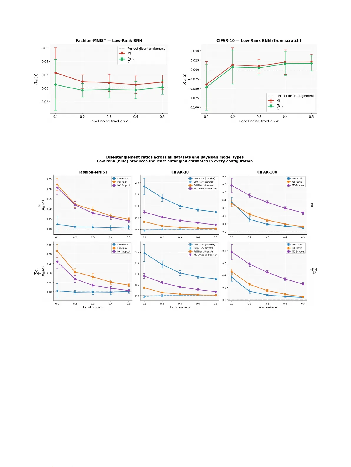
Not Just Ho w Much, But Wher e: Decomposing Epistemic Uncertainty into P er -Class Contrib utions Mame Diarra T oure 1 David A. Stephens 1 1 Department of Mathematics and Statistics , McGill Univ ersity Abstract In safety-critical classiﬁcation, the cost of failure is often asymmetric. Y et Bayesian deep learning sum- marises epistemic uncertainty with a single scalar , mutual information (MI), which cannot distinguish whether a model’ s ignorance in volv es a benign or safety-critical class. W e decompose MI into a per- class vector C k ( x ) = σ 2 k / (2 µ k ) , with µ k = E [ p k ] and σ 2 k =V ar[ p k ] across posterior samples. The de- composition follo ws from a second-order T aylor expansion of the entropy; the 1 /µ k weighting cor- rects boundary suppression and makes C k compa- rable across rare and common classes. By construc- tion P k C k ≈ MI , and a companion ske wness di- agnostic ﬂags inputs where the approximation de- grades. After characterising the axiomatic proper - ties of C k , we validate it on three tasks: (i) selecti ve prediction for diabetic retinopathy , where critical- class C k reduces selecti ve risk by 34.7% o ver MI and 56.2% ov er variance baselines; (ii) out-of- distribution detection on clinical and image bench- marks, where P k C k achie ves the highest A UROC and the per -class view e xposes asymmetric shifts in visible to MI; and (iii) a controlled label-noise study in which P k C k shows less sensitivity to injected aleatoric noise than MI under end-to-end Bayesian training, while both metrics de grade un- der transfer learning. Across all tasks, the quality of the posterior approximation shapes uncertainty at least as strongly as the choice of metric, suggest- ing that how uncertainty is propagated through the network matters as much as ho w it is measured. 1 INTR ODUCTION Deep learning classiﬁers deployed in safety-critical domains operate in en vironments where the cost of failure is asym- metric : missing a sight-threatening retinal condition is cate- gorically different from a f alse positiv e; auto-allowing hate speech carries risks that auto-blocking benign content does not. Bayesian deep learning addresses this by maintaining a posterior over model parameters, enabling principled decom- position of predictiv e uncertainty into aleatoric (irreducible data noise) and epistemic (model ignorance, reducible with data) components. The foundational decomposition w as for- malised by Kendall and Gal [2017] for vision tasks and by Depeweg et al. [2018] for latent-variable models via the law of total variance; Lakshminarayanan et al. [2017] established deep ensembles as a scalable alternative to varia- tional inference, with Gustafsson et al. [2020] demonstrating empirically that ensembles provide more reliable, better- calibrated uncertainty estimates than MC dropout across synthetic-to-real transfer benchmarks. All of these methods, howe ver , summarise epistemic un- certainty with a single scalar per input : the mutual infor- mation I ( y ; ω | x ) = H ( µ ) − E [ H ( p )] [Houlsby et al., 2011, Gal and Ghahramani, 2016]. This scalar rev eals how uncertain the model is, b ut not whic h classes are dri ving that uncertainty , a distinction that matters because model ignorance is rarely distributed uniformly across the label space. A scalar MI of 0 . 3 nats carries very different impli- cations depending on whether the confusion in volves two benign classes or a benign and a safety-critical one. Recent work has approached the per-class direction from se veral angles, each with a speciﬁc limitation (detailed com- parison in Appendix A). Sale et al. [2024] introduced a label- wise frame work reducing K -class problems to K binary sub-problems, with per-class epistemic variance EU k = V ar(Θ k ) satisfying strong axiomatic properties [W immer et al., 2023]; howe ver , raw v ariance suffers from boundary suppr ession , the constraint V ar[ p k ] ≤ µ k (1 − µ k ) forces it to v anish for rare classes re gardless of actual posterior disagreement. Dirichlet-based approaches [Sensoy et al., 2018, Malinin and Gales, 2018, Duan et al., 2024] produce per-class epistemic covariances in a single forward pass, but impose a strong distrib utional assumption on the proba- bility simplex. Dataset-le vel methods [Baltaci et al., 2023, Khan et al., 2019] address class imbalance and dif ﬁculty but conﬂate aleatoric and epistemic components and can- not provide input-le vel attribution. Scalar epistemic metrics, including B ALD [Houlsby et al., 2011] for acti ve learning and the v ariance-MI connection of Smith and Gal [2018], remain agnostic to class identity . Mucsányi et al. [2024] observed that aleatoric and epistemic estimates are often rank-correlated; de Jong et al. [2026] prov e this is a neces- sary consequence of estimator validity , shifting the deﬁning criterion from decorrelation to ortho gonality , a property that no current method fully achiev es. In summary , no existing method pro vides an input-speciﬁc, normalised per-class epistemic vector with a direct additi ve connection to MI. W e introduce C ( x ) = [ C 1 ( x ) , . . . , C K ( x )] ⊤ , where C k ( x ) = 1 2 V ar[ p k ]( x ) / µ k ( x ) is deri ved from a second- order T aylor approximation of MI (Section 2). The 1 /µ k normalization arises naturally from the entropy Hessian and counteracts boundary suppression; by construction, P k C k ( x ) ≈ I ( y ; ω | x ) , so each C k attributes a well- deﬁned share of total epistemic uncertainty to class k . Contributions. (1) W e deriv e C ( x ) from the T aylor ex- pansion of MI (Section 2.1), characterise its axiomatic prop- erties relativ e to W immer et al. [2023] (Section 2.4), and introduce a sk ewness diagnostic that ﬂags when the approxi- mation degrades (Section 2.5). (2) W e v alidate C ( x ) across three tasks: selectiv e prediction with class-speciﬁc deferral for diabetic retinopathy (Section 3), OoD detection where per-class contributions rev eal asymmetric distributional shift (Section 4), and a controlled disentanglement study show- ing that P k C k is less sensitiv e to injected label noise than MI under end-to-end Bayesian training, while both metrics degrade substantially under transfer learning (Section 5) 1 . 2 PER-CLASS EPISTEMIC UNCER T AINTY W e decompose MI into a K -dimensional vector C ( x ) via second-order T aylor expansion of the entropy . Each compo- nent C k quantiﬁes class k ’ s epistemic contribution, and the sum approximates MI. Setup and Notation Consider a K -class classiﬁer with input x . W e perform S stochastic forward passes (e.g., MC dropout, posterior sampling, or ensemble mem- bers), each producing a probability vector p ( s ) ( x ) = 1 Concurrently , de Jong et al. [2026] show that pretrained deep ensembles exhibit worse A U/EU disentanglement than models trained from scratch, a conclusion we reach independently in Sec- tion 5 via both the de gradation of the C k approximation and in- creased A U/EU entanglement under transfer learning. softmax( z ( s ) ( x )) ∈ ∆ K − 1 , where z ( s ) denotes the log- its from pass s . The Monte Carlo estimates of the mean and cov ariance are: µ ( x ) = 1 S P S s =1 p ( s ) ( x ) , (1) Co v[ p ] = 1 S − 1 P S s =1 ( p ( s ) − µ )( p ( s ) − µ ) ⊤ , (2) with diagonal elements V ar[ p k ] = 1 S − 1 P s ( p ( s ) k − µ k ) 2 . Throughout, we rely on the standard decomposition H ( µ ) | {z } T otal = E [ H ( p )] | {z } Aleatoric + H ( µ ) − E [ H ( p )] | {z } Epistemic ( I ) , (3) where H ( p ) = − P k p k log p k is the Shannon entropy and the epistemic term equals the mutual information I ( y ; ω | x ) . 2.1 FR OM SCALAR MI TO A PER-CLASS DECOMPOSITION Our strategy is to approximate E [ H ( p )] via a T aylor ex- pansion around µ , which yields an expression for MI that decomposes additiv ely over classes. Lemma 2.1 (Entropy Deri vati ves) . The Shannon entr opy H ( p ) = − P k p k log p k satisﬁes ∂ H ∂ p k = − 1 − log p k , ∂ 2 H ∂ p k ∂ p j = − δ kj p k , ∂ 3 H ∂ p 3 k = 1 p 2 k . (4) wher e δ kj is the Kr onecker delta ( δ kj = 1 if k = j , 0 otherwise). The Hessian is diagonal and negati ve semideﬁnite on the interior of the simplex. The diagonal Hessian is what mak es a per-class decomposition possible: there are no cross-class terms at second order , so the quadratic approximation splits cleanly ov er classes. Theorem 2.2 (MI Approximation 2 ) . Let p ( s ) ∼ Q with mean µ = E Q [ p ] and per-class variance V ar[ p k ] . Then E Q [ H ( p )] ≈ H ( µ ) − 1 2 K X k =1 V ar[ p k ] µ k , (5) with r emainder O ( E [ ∥ p − µ ∥ 3 ]) , and consequently I ( y ; ω | x ) ≈ 1 2 K X k =1 V ar[ p k ]( x ) µ k ( x ) . (6) The simplex constraint forces Co v[ p ] to hav e rank at most K − 1 , coupling the K components; this does not in validate the trace formula. See Appendix B.1 for proof. 2 Smith and Gal [2018] also exploit a T aylor expansion to relate softmax variance to MI, but expand the logarithm log p k rather than the entropy function H ( p ) itself (their Section 3.2, Eq. 10). This yields a class- aver aged variance 1 K P k V ar[ p k ] with equal weights per class, whereas e xpanding the entropy via its Hessian yields the curvature- weighted sum 1 2 P k V ar[ p k ] /µ k , in which the 1 /µ k factor enables per -class attribution. 2.2 PER-CLASS EPISTEMIC UNCER T AINTY VECTOR The additiv e structure of (6) invites a natural deﬁnition. Deﬁnition 2.3 (Per-Class Epistemic Uncertainty) . For a K -class classiﬁer with mean µ ( x ) and per-class vari- ance V ar[ p k ]( x ) from S stochastic forward passes, de- ﬁne the per-class epistemic uncertainty vector C ( x ) = [ C 1 ( x ) , . . . , C K ( x )] ⊤ with C k ( x ) := 1 2 V ar[ p k ]( x ) µ k ( x ) , (7) In practice, we add ε = 10 − 10 to the denominator for numer- ical stability . 3 When µ k = 0 across all passes, V ar[ p k ] = 0 and C k = 0 trivially . By construction, the vector satisﬁes K X k =1 C k ( x ) ≈ I ( y ; ω | x ) . (8) so each C k attributes a well-deﬁned share of total epistemic uncertainty to class k , providing the localisation that scalar MI lacks. 2.3 WHY V ARIANCE ALONE F AILS: BOUND AR Y SUPPRESSION A natural alternati ve to C k would be to use the raw v ariance V ar[ p k ] as a per-class epistemic measure, as proposed by Sale et al. [2024]. Howe ver , variance on a bounded interval exhibits a structural limitation near the simplex boundary that the 1 /µ k normalisation in (7) is designed to address. Lemma 2.4 (V ariance Bound on the Simplex) . F or any class k with mean pr ediction µ k ∈ [0 , 1] : V ar[ p k ] ≤ µ k (1 − µ k ) . (9) Consequently , V ar[ p k ] → 0 as µ k → 0 or µ k → 1 , r egar d- less of the de gr ee of model disagr eement in lo git space. See Appendix B.2. This bound rev eals a concrete problem: for a class with µ k ≈ 0 . 01 , variance is capped at roughly 0 . 01 e ven if the model’ s stochastic passes exhibit maximal disagreement about that class. The following lemma sho ws that C k corrects exactly this pathology . 3 The ratio V ar[ p k ] /µ k coincides with the index of disper- sion [Cox and Le wis, 1966] (Fano factor [F ano, 1947]). Here the 1 2 prefactor and the 1 /µ k weighting both emerge from the en- tropy T aylor expansion, so the components sum to a well-deﬁned information-theoretic quantity . Lemma 2.5 (Boundary Behaviour of C k ) . Under the same conditions: C k = 1 2 V ar[ p k ] µ k ≤ 1 2 (1 − µ k ) , (10) which appr oaches 1 2 (not zer o) as µ k → 0 . While V ar[ p k ] is crushed to zer o near the simplex boundary , C k r etains a non-vanishing upper bound. See Appendix B.2. The mechanism is not ad hoc: the Hessian entry − 1 /µ k grows large when µ k is small, so a gi ven amount of prob- ability v ariance carries more information-theoretic weight for lo w-probability classes. Con versely , when µ k → 1 the curvature v anishes and C k → 0 , the correct limit. This ren- ders C k comparable across classes with very dif ferent base rates, a property V ar[ p k ] lacks by construction. 2.4 AXIOMA TIC AN AL YSIS Having described both the diagonal vector C ( x ) and the off-diagonal co v ariance structure, we now examine whether C ( x ) satisﬁes standard properties of epistemic uncertainty measures. W immer et al. [2023] propose a set of axioms formalising desirable behaviour for epistemic uncertainty measures. W e assess the aggregate EU approx ( Q ) = P k C k against ﬁ ve of these axioms, where Q denotes the second- order distrib ution ov er probability vectors p with mean µ = E Q [ p ] . Theorem 2.6 (Axiomatic Proﬁle) . The appr oximate epis- temic uncertainty EU approx ( Q ) = P K k =1 C k satisﬁes ax- ioms A0, A1, and A3, and violates A2 and A5 of W immer et al. [2023]. See Appendix B.3 for details and pr oof. The violations of A2 and A5 are not artefacts of the approx- imation; they are inherited from MI itself [W immer et al., 2023]. More re vealing is the relationship between A5 and boundary suppression: Corollary 2.7 (A5 V iolation as Boundary Correction) . The violation of A5 is the pr ecise mec hanism that counteracts boundary suppr ession. A5 r equires EU to be insensitive to µ k ; but by Lemma 2.5, sensitivity to µ k is what pr events C k fr om vanishing as µ k → 0 . This trade-off clariﬁes the design space: the label-wise vari- ance EU k = V ar(Θ k ) of Sale et al. [2024] satisﬁes A5 but pays the cost of boundary suppression. Our C k sacriﬁces A5 to preserve comparability across classes with different base rates, a trade-off we argue is favourable in safety-critical settings where rare classes matter most. Remark 2.8 (A3 vs. Exact MI) . Unlike exact MI, which W immer et al. [2023] show violates A3 in general (their Proposition 4), P k C k satisﬁes it strictly . Since the sum is linear in each V ar[ p k ] with ﬁxed positiv e coefﬁcients 1 / (2 µ k ) , any mean-preserving spread necessarily increases it, so greater model disagreement alw ays produces greater epistemic uncertainty . 2.5 RELIABILITY DIA GNOSTIC VIA SKEWNESS The same 1 /µ k factor that corrects boundary suppression also controls where the T aylor expansion breaks do wn. As µ k → 0 , the curvature | ∂ 2 H /∂ p 2 k | = 1 /µ k div erges, and the quadratic approximation becomes increasingly sensitive to higher-order terms. A natural question is: when can we trust C k ? W e answer this by examining the ne xt term in the expansion. Lemma 2.9 (Third-Order Correction) . Including the thir d- or der term fr om Lemma 2.1, the expected entr opy satisﬁes E [ H ( p )] ≈ H ( µ ) − 1 2 X k V ar[ p k ] µ k + 1 6 X k m 3 ,k µ 2 k , (11) wher e m 3 ,k = E [( p k − µ k ) 3 ] is the third central moment, estimated as ˆ m 3 ,k = 1 S P S s =1 ( p ( s ) k − µ k ) 3 . W e use the third-order term as a diagnostic rather than a correction. Including it yields C (3) k = 1 2 V ar[ p k ] /µ k − 1 6 m 3 ,k /µ 2 k , b ut the 1 /µ 2 k singularity can dri ve this quan- tity negati ve for right-skewed distrib utions near the simplex boundary , violating non-negati vity (A0). More fundamen- tally , adding T aylor terms improv es accuracy only when posterior samples are tightly concentrated around the mean, which is precisely not the high-uncertainty regime where the metric matters most. The ske wness ratio ρ k (Section 2.5) instead ﬂags when the second-order approximation is unre- liable, without compromising the guarantees of C k . Deﬁnition 2.10 (Skewness Diagnostic) . For each class k with V ar[ p k ] > 0 , deﬁne the reliability indicator ρ k ( x ) = | m 3 ,k | 3 µ k · V ar[ p k ] . (12) T o see why this is the right ratio, observe that the second- order contribution to MI from class k is 1 2 V ar[ p k ] /µ k , while the third-order correction is 1 6 | m 3 ,k | /µ 2 k . Their ratio is 1 6 | m 3 ,k | /µ 2 k 1 2 V ar[ p k ] /µ k = | m 3 ,k | 3 µ k · V ar[ p k ] = ρ k . (13) When ρ k ≪ 1 , the third-order correction is negligible rel- ativ e to C k , and the approximation is reliable for class k . When ρ k is appreciable (e.g., ρ k > 0 . 3 ), the second-order approximation is degrading, and C k should be interpreted with caution. The diagnostic is computable from the same S stochastic passes at negligible additional cost and can be reported alongside C ( x ) . Off-diagonal structure and the CBEC metric. While C ( x ) captures diagonal variance per class, the empiri- cal covariance Co v[ p ] encodes complementary informa- tion about pairwise confusion . A strongly ne gati ve entry Co v[ p i , p j ] ≪ 0 means that probability mass ﬂows system- atically between classes i and j across stochastic passes: the model is activ ely trading one for the other rather than being dif fusely uncertain. In safety-critical settings this directional signal matters: a model torn between a safe and a critical class is qualitativ ely dif ferent from one torn between two safe classes, yet both can produce identical P k C k . When the ske wness diagnostic (Section 2.5) ﬂags unreliable C k for rare critical classes ( µ k ≈ 0 ), we gate their product by the empirical negati ve correlation between safe and critical classes: CBEC ( x ) = X i ∈S X j ∈C p C i · C j · max(0 , − ρ ij ) , (14) where S and C are the safe and critical class sets and ρ ij is the empirical Pearson correlation of p i and p j across the S forward passes. Three design choices interact. The geomet- ric mean p C i · C j requires both classes to carry elev ated epistemic uncertainty: single-class inﬂation is dampened by the square root, and if either class is certain the product van- ishes. The corr elation gate max(0 , − ρ ij ) ﬁlters coinciden- tal co-elev ation: the score is nonzero only when MC draws show the model acti vely exchanging probability between the two classes, a T aylor-free condition that remains reli- able ev en when C k degrades. The r estricted domain S × C focuses the sum e xclusiv ely on cross-boundary confusion, excluding within-safe and within-critical co-elev ation that carry no deferral signal. T ogether , these properties make CBEC the preferred fallback when ρ k > 0 . 3 for critical classes; C crit_max remains the primary metric when the T ay- lor approximation is reliable. 3 SELECTIVE PREDICTION FOR DIABETIC RETINOP A THY W e ev aluate C ( x ) on selective prediction [Geifman and El-Y ani v, 2017] for diabetic retinopathy (DR) grading, a task where the cost of failure is acutely asymmetric: missing a sight-threatening retinopathy carries irre versible conse- quences, while a f alse positiv e triggers only a follow-up examination. 3.1 EXPERIMENT AL SETUP Data. W e pool three public DR grading benchmarks: Eye- P A CS [Cuadros and Bresnick, 2009], APTOS 2019 [Asia Paciﬁc T ele-Ophthalmology Society, 2019], and Messidor- 2 [Decencière et al., 2014], totalling 39 , 970 colour fun- dus photographs. The International Clinical DR Sev erity Scale [W ilkinson et al., 2003] deﬁnes ﬁ ve grades; we con- solidate the tw o most severe into a single grade because both require urgent referral. The resulting four -class distribution places Grades 2–3 as critical ( C = { 2 , 3 } , requiring treat- ment) and Grades 0–1 as safe ( S = { 0 , 1 } ); data are split patient-stratiﬁed into train/v al/test with no patient leakage (full details in Appendix D.1). Model. W e construct a fully Bayesian EfﬁcientNet- B4 [T an and Le, 2019] using the low-rank variational in- ference framew ork of T oure and Stephens [2026], with a scale-mixture Gaussian prior ( π = 0 . 5 ) and KL annealing. Full architectural details are in Appendix D.2. Inference and e valuation. Uncertainty is estimated from S = 30 stochastic forward passes through the poste- rior . Our primary safety metric is the critical false neg- ative rate (Critical FNR, Appendix C.8): among critical- class samples retained at a gi ven coverage le vel, the frac- tion misclassiﬁed as safe. W e summarise performance across cov erage le vels via the area under the selecti ve risk curve (A USC) [El-Y aniv and W iener, 2010], with 95% CIs from 200 bootstrap resamples. On the test set, the Bayesian model achiev es accuracy 0 . 8 and quadratic weighted kappa 0 . 65 ; per-class performance in Appendix D.3. 3.2 DEFERRAL POLICIES W e compare 10 deferral policies across four families (T a- ble 1; formal deﬁnitions in Appendix C). T able 1: Deferral policies e valuated. Higher score = defer . C = { 2 , 3 } , S = { 0 , 1 } . Family Policy Score Scalar Entropy H [ ¯ p ] MI H [ ¯ p ] − E [ H [ p ( s ) ]] MaxProb 1 − max k µ k Sale_EU_global P k σ 2 k Per-class variance V ar_crit max k ∈C σ 2 k Sale_EU_crit P k ∈C σ 2 k Per-class MI OvA_MI P k ∈C MI bin k Per-class C k (proposed) C crit_sum P k ∈C C k C crit_max max k ∈C C k CBEC Eq. 14 Scalar baselines are class-agnostic; per-class variance tar- gets critical classes via raw σ 2 k but is confounded by µ k (Lemma 2.4); OvA_MI computes binary MI per critical class. Our three proposed metrics build on P k C k ≈ I (Section 2.2): C crit_max giv es the sharpest signal when C k estimates are reliable ( ρ k < 0 . 3 ); C crit_sum is a smoother alternativ e; CBEC (Eq. 14) gates safe–critical pairs by em- pirical negati ve correlation for robustness when ske wness degrades C k . 3.3 RESUL TS Theory validation. Before ev aluating downstream perfor- mance, we verify the additi ve decomposition (8) : P k C k and e xact MI achie ve Pearson r = 0 . 988 and Spearman r = 0 . 998 across all 7 , 948 test samples (Figure 4), con- ﬁrming the second-order approximation preserv es epistemic uncertainty rankings. The ske wness diagnostic (Section 2.5) shows C k is reliable ( ρ k < 0 . 3 ) for > 94% of safe-class samples and 82% / 63% of Grade 2/3 respectively; full distri- butions in Appendix D.4. Main results. T able 2 reports A USC and Critical FNR at 80% cov erage with bootstrap CIs. C crit_max achiev es the lowest A USC ( 0 . 285 ), reducing the area under the selec- tiv e risk curv e by 34.7% relati ve to MI ( 0 . 436 , p < 0 . 005 ) and by 56.2% relati ve to Sale_EU_crit ( 0 . 650 , p < 0 . 005 ). At the clinically relevant 80% cov erage operating point, C crit_max achie ves FNR 0 . 302 , compared to 0 . 339 for MI and 0 . 409 for Sale_EU_crit. Figure 1 visualises these results: C crit_max dominates across the full coverage range (left), with non-ov erlapping bootstrap interquartile ranges against scalar baselines (right). The impro vement o ver ra w v ariance is especially striking. Sale_EU_crit and V ar_crit (A USC 0 . 650 and 0 . 606 ) perform worse than entr opy ( 0 . 604 ), con- ﬁrming that boundary suppression (Lemma 2.4) se verely confounds unnormalised variance for critical classes with µ k ≈ 0 . 06 . The 1 /µ k normalisation in C k corrects precisely this: Grade 3 has mean probability ∼ 0.06, giving entropy curvature ∼ 17, so ev en small variance there carries large information-theoretic weight. This normalisation beneﬁt is robust to the choice of inference method: a deep ensemble [Lakshminarayanan et al., 2017] of ﬁve members yields C crit_max A USC 0 . 390 vs. 0 . 447 for Sale_EU_crit ( 12 . 9% reduction; Appendix D.12). T able 2: Selective prediction for DR grading (Bayesian EfﬁcientNet-B4, S =30 ). A USC integrates Critical FNR ov er all co verages (lower = safer). Bold = best; CIs: 200 bootstrap resamples. Family Policy A USC (Critical FNR) ↓ Critical FNR @80% ↓ Scalar Entropy 0 . 604 ± 0 . 022 0 . 401 ± 0 . 016 MI 0 . 436 ± 0 . 019 0 . 339 ± 0 . 014 MaxProb 0 . 639 ± 0 . 022 0 . 439 ± 0 . 017 Sale_EU_global 0 . 457 ± 0 . 018 0 . 341 ± 0 . 015 Per-class v ar . V ar_crit 0 . 606 ± 0 . 014 0 . 379 ± 0 . 016 Sale_EU_crit 0 . 650 ± 0 . 013 0 . 409 ± 0 . 016 Per-class MI OvA_MI 0 . 452 ± 0 . 017 0 . 367 ± 0 . 015 Per-class C k (proposed) C crit_sum 0 . 327 ± 0 . 017 0 . 321 ± 0 . 014 C crit_max 0 . 285 ± 0 . 016 0 . 302 ± 0 . 013 CBEC 0 . 416 ± 0 . 020 0 . 335 ± 0 . 014 Interpr etability: Error Signatures. A distinctive adv an- tage of C ( x ) ov er scalar MI is that it reveals the struc- tur e of model confusion. Figure 2 shows that catastrophic misses (Grade 3 predicted as Grade 0) and severity un- derestimates (Grade 3 predicted as Grade 2) ha ve nearly Figure 1: Selective prediction for DR. Left: Critical FNR vs. cov erage; C crit_max dominates all baselines across the full range. Right: Bootstrap A USC distrib ution ( n =200 ); C k -based policies (red/orange) show non-overlapping in- terquartile ranges against scalar baselines (grey). identical scalar MI ( 0 . 024 vs. 0 . 027 nats) but very differ - ent C k signatures. The catastrophic miss concentrates epis- temic mass on C 2 , identifying Grade 2 as the bottleneck of confusion, while the sev erity underestimate elev ates C 0 , indicating doubt about healthy status. These qualitati vely different failure modes, in visible to scalar metrics, suggest distinct remediation strategies; the epistemic confusion ma- trix (Appendix D.10) further conﬁrms that cross-boundary confusion is 2 . 7 × stronger than within-group confusion, validating the clinical partition (detailed analysis in Ap- pendix D.9). Robustness acr oss inference methods. T o test robust- ness to the posterior approximation, we repeat the ev alu- ation using standard MC dropout [Gal and Ghahramani, 2016] ( p =0 . 3 , S =30 ). The ranking changes markedly: CBEC achiev es the lo west A USC ( 0 . 197 ± 0 . 012 , winning 100% of bootstrap samples), a 53.6% reduction over MI ( 0 . 425 ± 0 . 024 ), while C crit_max drops to 0 . 419 . MC dropout is kno wn to produce regions of spurious conﬁdence where the approximate posterior underestimates uncertainty [Smith and Gal, 2018]. In our framew ork, this inﬂates ρ k for critical classes, degrading the T aylor approximation underlying C k while leaving CBEC’ s correlation gate intact. A deep en- semble of ﬁ ve members conﬁrms the pattern: CBEC ag ain achie ves the lowest A USC ( 0 . 223 ), ev en though C k reliabil- ity remains high ( ρ k < 0 . 3 for > 85% of Grade 3 samples), indicating that the correlation gate captures cross-boundary structure beyond what single-class tar geting provides. This conﬁrms the intended complementarity: C crit_max is the pri- mary metric under well-calibrated posteriors; CBEC pr o- vides a r obust alternative acr oss infer ence r e gimes. Full results in Appendix D.11 and D.12. 4 OUT -OF-DISTRIB UTION DETECTION W e e valuate the per-class epistemic uncertainty metric on out-of-distribution (OoD) detection, where elev ated epis- temic uncertainty should signal distributional shift. Figure 2: Epistemic signatures for Grade 3 errors with sim- ilar MI b ut distinct C k patterns. Left: Catastrophic miss ( 3 → 0 , MI = 0.024) concentrates on C 2 . Centre: Sever - ity underestimate ( 3 → 2 , MI = 0.027) elev ates C 0 . Right: Grouped comparison showing the C k ﬁngerprints differ markedly despite similar MI, the catastrophic miss (red) peaks at C 2 while the sev erity error (dark red) peaks at C 0 . 4.1 SETUP Datasets. W e consider two OoD detection tasks: (1) F ash- ionMNIST [Xiao et al., 2017] → KMNIST [Clanuw at et al., 2018], a 10-class image task (50k/10k train/test, 10k OoD); and (2) MIMIC-III ICU [Johnson et al., 2016] → Newborn , binary mortality prediction on 44 tabular features (40k/4.5k train/test, 5.4k OoD). Model. Both tasks use low-rank Bayesian neural networks with Gaussian posteriors. FashionMNIST : two hidden layers (1200 units, rank 25), S =50 MC samples. MIMIC-III: two hidden layers (128 units, rank 15), S =512 MC samples, with class-weighted training to address mortality imbalance (8.6% pre valence). See Appendix E.2 for full architectural and training details. Metrics. W e compare four uncertainty scores: neg ativ e maximum softmax probability [Hendrycks and Gimpel, 2017], MI, E U var = P k σ 2 k , and our proposed P k C k . Per- formance is measured by A UR OC(ID samples labelled 0, OoD samples labelled 1); results are mean ± std ov er 5 seeds. 4.2 RESUL TS T able 3 summarises OoD detection performance. P k C k achiev es the highest A UROC on both datasets: 0 . 735 on FashionMNIST v ersus 0 . 724 for MI, and 0 . 815 on MIMIC- III versus 0 . 802 for MI. The OoD-to-ID ratio column rev eals the mechanism: on FashionMNIST , P k C k ampliﬁes the distributional shift signal to 6 . 43 × versus 5 . 92 × for MI. On FashionMNIST , this ef fect is predicted by Lemma 2.9: the gap P k C k − MI ≈ 1 6 P k m 3 ,k /µ 2 k grows with poste- rior ske wness, and OoD samples produce higher ske wness diagnostic ρ k than ID samples across all ten classes (Ap- pendix E.6, Figure 14). On MIMIC-III the picture is more nuanced: the surviv al class ( k =0 ) follows the e xpected pat- tern ( ρ OOD 0 > ρ ID 0 , median shift +43% ), but the mortality class ( k =1 ) re verses because near-zero µ 1 for ne wborns col- lapses V ar[ p 1 ] faster than 1 /µ 1 can compensate, concentrat- ing the third-order signal entirely in class 0 (Appendix E.6). The unnormalised baseline E U var underperforms MI on both datasets despite matching its ratio on FashionMNIST ( 5 . 92 × ): without mean-normalisation, raw variance σ 2 k is bounded above by µ k (1 − µ k ) , compressing the dynamic range of uncertainty scores. On MIMIC-III E U var achiev es the highest ratio ( 1 . 71 × ) yet the lowest A UR OC among epistemic measures. A high mean ratio does not imply good separability: A UR OC depends on the full distributional over - lap, and the un-normalised v ariance sum concentrates both ID and OoD scores near zero with a shared heavy tail, so the numerically large mean shift is swamped by within- group spread (Appendix E.5, Figure 12). This pattern is consistent across inference methods: a deep ensemble repli- cates the same ranking ( P k C k =0 . 753 > MI =0 . 752 > E U var =0 . 750 ) on MIMIC-III, with E U var again achiev- ing the highest ratio ( 2 . 72 × ) and the lowest A UR OC (Ap- pendix E.7). T able 3: OoD detection: A UR OC and OoD/ID mean- uncertainty ratio. Best in bold . FashionMNIST → KMNIST MIMIC-III ICU → Newborn Family Method A UROC ↑ Ratio ↑ A UR OC ↑ Ratio ↑ Baselines Neg. MSP 0 . 665 ± 0 . 013 2 . 07 0 . 688 ± 0 . 030 1 . 24 MI 0 . 724 ± 0 . 009 5 . 92 0 . 802 ± 0 . 004 1 . 61 E U var 0 . 710 ± 0 . 010 5 . 92 0 . 778 ± 0 . 015 1 . 71 Proposed P k C k 0 . 735 ± 0 . 009 6 . 43 0 . 815 ± 0 . 017 1 . 62 Per -class decomposition. On the binary MIMIC-III task, the decomposition P k C k = C 0 + C 1 rev eals that distrib u- tional shift affects the two classes asymmetrically ( 2 . 15 × for surviv al vs. 1 . 30 × for mortality): the larger OoD signal resides in the non-critical class, so C 1 -only yields A UR OC 0 . 740 , well below P k C k at 0 . 815 . On FashionMNIST the pattern is the opposite: all ten per -class C k values increase uniformly from ID to OoD (Appendix E.4, Figure 11), con- sistent with KMNIST inducing a structural rather than se- mantic shift that does not concentrate on any subset of classes. T ogether , these two cases illustrate a task-dependent trade-off: critical-class targeting impro ves selecti ve predic- tion (Section 3) but all-class aggreg ation is necessary for OoD detection, where the locus of distributional shift is not kno wn a priori and can be either asymmetric (MIMIC- III) or uniform (FashionMNIST). Full per-class results in Appendix E.3. 5 EPISTEMIC SENSITIVITY TO D A T A QU ALITY W e assess whether P k C k remains insensitiv e to irreducible aleatoric noise under controlled label-noise injection. 5.1 SETUP Data. W e use Fashion-MNIST ( K =10 , 60,000 images) and CIF AR-10 ( K =10 , 50,000 images) [Krizhe vsky et al., 2009]. For each dataset we inject symmetric label noise at rates α ∈ { 0 . 1 , 0 . 2 , 0 . 3 , 0 . 4 , 0 . 5 } : a fraction α of training labels is replaced uniformly at random, increasing aleatoric uncertainty without altering the input distribution. Model. W e compare end-to-end Bayesian training with transfer learning using lo w-rank Gaussian posteriors ( S =50 MC samples). Fashion-MNIST : fully Bayesian; two hid- den layers ( 400 units, rank 15 ). CIF AR-10: (i) end-to- end Conv 32 → 64 → 128 , rank 32 ; (ii) frozen ResNet-18 with Bayesian head. Full details, alternativ e posteriors, and CIF AR-100 results in Appendix F .1. Protocol. For each noise le vel α we compute the mean aleatoric uncertainty ¯ U a ( α ) = 1 N P i E [ H ( p i )] and the mean epistemic uncertainty ¯ U e ( α ) using either MI or P k C k ov er the clean test set. The relati ve disentanglement ratio R rel ( α ) = ( ¯ U e ( α ) − ¯ U e (0)) / ¯ U e (0) ( ¯ U a ( α ) − ¯ U a (0)) / ¯ U a (0) (15) measures the percentage increase in epistemic uncertainty per percentage increase in aleatoric uncertainty . R rel = 0 indicates perfect disentanglement; R rel = 1 indicates full entanglement; v alues above 0 . 3 signal substantial contam- ination (see Appendix F .2 for the motiv ation behind the relativ e formulation over the absolute ratio). 5.2 RESUL TS T able 4 reports | R rel | for low-rank Bayesian models un- der three conﬁgurations. Under end-to-end training, both metrics are near -perfectly disentangled ( | R rel | ≪ 0 . 3 ev- erywhere), conﬁrming that end-to-end Bayesian training with low-rank posteriors is the regime that produces the least entangled uncertainty estimates. It is also the regime under which the second-order T aylor expansion most ac- curately approximates exact MI: at α =0 , P k C k / MI is 1 . 00 × on Fashion-MNIST and 1 . 02 × on CIF AR-10 (T a- ble 22). P k C k achiev es lo wer | R rel | in 9 of the 10 end- to-end conditions, the exception being CIF AR-10 at α =0 . 1 where both values remain belo w 0 . 05 . The rightmost block contrasts the same model type and dataset (CIF AR-10, low- rank) under transfer learning: ratios jump to 0 . 74 – 1 . 97 , an order-of-magnitude degradation that isolates the training regime as the causal factor . The posterior approximation matters as much as the metric. T able 4 identiﬁes training regime as a ke y factor . Under end-to-end training, posterior e xpressiv eness tracks entanglement: on Fashion-MNIST the lo w-rank model achiev es a mean | R rel | below 0 . 01 for both metrics, while T able 4: | R rel ( α ) | for low-rank Bayesian models. Lower is better; † = P k C k less entangled. The ﬁrst two blocks use end-to-end training (e2e); the third uses a frozen ResNet-50 backbone with a low-rank Bayesian head (TL). FMNIST (e2e) CIF AR-10 (e2e) CIF AR-10 (TL) α MI P k C k MI P k C k MI P k C k 0.1 0.023 0 . 005 † 0 . 040 0.047 1 . 830 1.970 0.2 0.010 0 . 003 † 0.012 0 . 007 † 1 . 344 1.435 0.3 0.008 0 . 002 † 0.009 0 . 004 † 0 . 991 1.039 0.4 0.005 0 . 003 † 0.020 0 . 016 † 0 . 832 0.868 0.5 0.009 0 . 002 † 0.020 0 . 017 † 0 . 737 0.760 the full-rank model reaches 0 . 11 (MI) / 0 . 10 ( P k C k ) and MC dropout 0 . 10 / 0 . 06 respectiv ely (Appendix F .2). T rans- fer learning disrupts this hierarchy: even the lo w-rank model produces | R rel | exceeding 0 . 73 on CIF AR-10, an order of magnitude worse than any end-to-end conﬁguration, be- cause the frozen backbone supplies features ne ver optimised for calibrated predictive v ariance. This suggests that the high entanglement reported by Mucsányi et al. [2024] re- ﬂects the training regime as much as the decomposition formula. When uncertainty is not propagated through the full network, none of the three posterior families we e v alu- ate can compensate, moti vating the sk ewness diagnostic of Section 2.5 to ﬂag such conﬁgurations. Across end-to-end settings (Figure 15), P k C k achiev es lower | R rel | than MI in 19 of 20 conditions. Under transfer learning both metrics degrade and MI edges ahead, coinciding with baseline ratios P k C k / MI abov e roughly 1 . 6 × (T able 22), i.e. where the T aylor residual is largest. Full transfer -learning results and an analysis of the rank constraint’ s effect on uncertainty scale appear in Appendix F .2. Sensitivity to class cardinality . On CIF AR-100 [Krizhevsk y et al., 2009], the 1 /µ k normalisation ampliﬁes contributions from lo w-probability classes, inﬂating P k C k relativ e to MI by 1 . 17 × for the low-rank model and 1 . 89 × for MC dropout. The O ( K 2 ) scaling analysis and mitigation strategies are detailed in Appendix F .3. 6 DISCUSSION AND CONCLUSION W e presented a per-class epistemic uncertainty decomposi- tion C ( x ) deriv ed from a second-order T aylor expansion of MI, where the 1 /µ k normalisation arises naturally from the entropy Hessian and counteracts boundary suppression. The decomposition reduces to a simple ratio of v ariance to mean per class, adds ne gligible cost to any posterior sampling pipeline, and closely tracks scalar MI by summation. The three e xperiments exposed a consistent theme: the value of C ( x ) lies not in being a better scalar summary but in enabling class-speciﬁc queries that scalar metrics cannot express. F or selectiv e prediction, targeting critical-class C k outperformed all scalar and v ariance-based baselines; for OoD detection, the per-class view re vealed that distribu- tional shift can concentrate asymmetrically across classes, a structure in visible to any aggreg ate score; for disentangle- ment, the decomposition provided a lens to diagnose when and why epistemic and aleatoric signals become entangled. A ﬁnding we did not anticipate is that the posterior ap- proximation shaped metric behaviour at least as strongly as the metric itself. Switching from variational inference to MC dropout rev ersed the ranking of our deferral policies, because dropout inﬂated ske wness precisely for the rare classes where the T aylor expansion is most sensiti ve. The disentanglement experiments sharpened this further: freez- ing a pretrained backbone and attaching a Bayesian head degraded A U/EU separation by o ver an order of magnitude compared to end-to-end training, e ven when the Bayesian component was identical. This raises a question for the gro w- ing literature on post-hoc Bayesian methods: if features are learned without any posterior objecti ve, the resulting vari- ance structure may not support meaningful epistemic attri- bution re gardless of the last-layer treatment. W e do not sug- gest post-hoc methods lack practical v alue, but the quality of their uncertainty outputs deserv es scrutin y commensurate with the attention giv en to their scalability . W e note sev eral limitations. The additi ve link P k C k ≈ I loosens under high ske wness over lo w-probability classes, since the third-order remainder scales as 1 /µ 2 k ; ρ k diagnoses but does not correct this, and the CBEC fallback requires do- main knowledge to deﬁne class partitions. The 1 /µ k normal- isation introduces O ( K 2 ) scaling of the aggregate, necessi- tating truncation or reweighting in high-cardinality settings, though the per-class v ector itself remains fully interpretable. All models use MFVI, lo w-rank Gaussian VI, MC dropout, or deep ensembles. Characterising ho w C k behav es under other approximate inference schemes such as Laplace ap- proximations [Daxberger et al., 2021] or stochastic weight av eraging [Maddox et al., 2019] is a natural next step. The decomposition is not tied to any speciﬁc posterior fam- ily or architecture. Future work includes extending C ( x ) to structured prediction tasks where class identity is less cleanly deﬁned, integrating it into acti ve learning acquisi- tion functions that target speciﬁc classes, and combining low-rank ensembles with per -class attribution for richer un- certainty proﬁles. More fundamentally , making end-to-end Bayesian training more practical and scalable strikes us as a more promising path than reﬁning post-hoc corrections, and the per-class decomposition is designed to complement that direction. 4 4 Code and trained models are a vailable in the supplementary material. References Asia Paciﬁc T ele-Ophthalmology Society . APT OS 2019 blindness detection. Kaggle Competition, 2019. URL https://www.kaggle.com/c/ aptos2019- blindness- detection . Zeynep Sonat Baltaci, K emal Oksuz, Selim K uzucu, Ki vanc T ezoren, Berkin Kerim K onar , Alpay Ozkan, Emre Akbas, and Sinan Kalkan. Class uncertainty: A measure to miti- gate class imbalance. arXiv pr eprint arXiv:2311.14090 , 2023. David M Blei, Alp K ucukelbir , and Jon D McAulif fe. V ari- ational inference: A re view for statisticians. Journal of the American statistical Association , 112(518):859–877, 2017. Charles Blundell, Julien Cornebise, K oray Ka vukcuoglu, and Daan Wierstra. W eight uncertainty in neural net- works. In Pr oceedings of the 32nd International Confer- ence on Machine Learning (ICML) , pages 1613–1622. PMLR, 2015. Robin Camarasa, Daniel Bos, Jeroen Hendrikse, Paul Ned- erkoorn, M. Eline K ooi, Aad van der Lugt, and Marleen de Bruijne. A quantitative comparison of epistemic uncer - tainty maps applied to multi-class segmentation. Machine Learning for Biomedical Imaging , 1(UNSURE2020): 1–39, September 2021. ISSN 2766-905X. doi: 10.59275/ j.melba.2021- ec49. URL http://dx.doi.org/10. 59275/j.melba.2021- ec49 . T arin Clanuwat, Mikel Bober-Irizar , Asanobu Kitamoto, Alex Lamb, Kazuaki Y amamoto, and David Ha. Deep learning for classical japanese literature. arXiv pr eprint arXiv:1812.01718 , 2018. David R. Cox and Peter A. W . Lewis. The Statistical Analy- sis of Series of Events . Methuen, London, 1966. Jorge Cuadros and George Bresnick. Eyepacs: an adaptable telemedicine system for diabetic retinopathy screening. J ournal of diabetes science and technology , 3(3):509–516, 2009. Erik Daxberger , Agustinus Kristiadi, Alexander Immer , Runa Eschenhagen, Matthias Bauer, and Philipp Hen- nig. Laplace redux–effortless bayesian deep learning. In Pr oceedings of the 35th International Confer ence on Neu- ral Information Pr ocessing Systems , pages 20089–20103, 2021. Ivo Pascal de Jong, Andreea Ioana Sburlea, Matthia Sabatelli, and Matias V aldenegro-T oro. Measuring or- thogonality as the blind-spot of uncertainty disentan- glement, 2026. URL 2408.12175 . Etienne Decencière, Xiwei Zhang, Guy Cazuguel, Bruno Lay , Béatrice Cochener , Caroline Trone, Philippe Gain, John-Richard Ordóñez-V arela, Pascale Massin, Ali Erginay , et al. Feedback on a publicly distrib uted im- age database: the messidor database. Imag e Analysis & Ster eology , pages 231–234, 2014. Stefan Depeweg, Jose-Miguel Hernandez-Lobato, Finale Doshi-V elez, and Steffen Udluft. Decomposition of un- certainty in bayesian deep learning for ef ﬁcient and risk- sensitiv e learning. In International confer ence on ma- chine learning , pages 1184–1193. PMLR, 2018. Ruxiao Duan, Brian Caffo, Harrison X. Bai, Haris I. Sair , and Craig Jones. Evidential uncertainty quantiﬁcation: A variance-based perspectiv e. In Pr oceedings of the IEEE/CVF W inter Conference on Applications of Com- puter V ision (W ACV) , pages 2132–2141, 2024. Ran El-Y ani v and Y air W iener . On the foundations of noise- free selectiv e classiﬁcation. JMLR , 11:1605–1641, 2010. Ugo Fano. Ionization yield of radiations. II. The ﬂuctuations of the number of ions. Physical Re view , 72(1):26–29, 1947. Y arin Gal and Zoubin Ghahramani. Dropout as a Bayesian approximation: Representing model uncertainty in deep learning. In Pr oceedings of the 33r d International Con- fer ence on Machine Learning (ICML) , pages 1050–1059. PMLR, 2016. Y arin Gal, Riashat Islam, and Zoubin Ghahramani. Deep Bayesian acti ve learning with image data. In Interna- tional confer ence on mac hine learning , pages 1183–1192. PMLR, 2017. Y onatan Geifman and Ran El-Y ani v . Selective classiﬁca- tion for deep neural networks. In Advances in Neural Information Pr ocessing Systems (NeurIPS) , volume 30, 2017. Fredrik K. Gustafsson, Martin Danelljan, and Thomas B. Schön. Evaluating scalable Bayesian deep learning meth- ods for rob ust computer vision. In Pr oceedings of the IEEE/CVF Confer ence on Computer V ision and P attern Recognition W orkshops (CVPRW) , pages 318–319, 2020. Dan Hendrycks and K evin Gimpel. A baseline for detecting misclassiﬁed and out-of-distribution e xamples in neural networks. In International Conference on Learning Rep- r esentations (ICLR) , 2017. Neil Houlsby , Ferenc Huszár , Zoubin Ghahramani, and Máté Lengyel. Bayesian activ e learning for classiﬁcation and preference learning. arXiv preprint , 2011. Alistair E. W . Johnson, T om J. Pollard, Lu Shen, Li-wei H. Lehman, Mengling Feng, Mohammad Ghassemi, Ben- jamin Moody , Peter Szolo vits, Leo Anthony Celi, and Roger G. Mark. MIMIC-III, a freely accessible critical care database. Scientiﬁc Data , 3(1):160035, 2016. Alex Kendall and Y arin Gal. What uncertainties do we need in Bayesian deep learning for computer vision? In Advances in Neural Information Pr ocessing Systems (NeurIPS) , volume 30, pages 5574–5584, 2017. Salman Khan, Munawar Hayat, Syed W aqas Zamir, Jianbing Shen, and Ling Shao. Striking the right balance with uncertainty . In Pr oceedings of the IEEE/CVF Confer ence on Computer V ision and P attern Recognition , pages 103– 112, 2019. Alex Krizhe vsky , Geoffre y Hinton, et al. Learning multiple layers of features from tiny images. 2009. Balaji Lakshminarayanan, Alexander Pritzel, and Charles Blundell. Simple and scalable predictiv e uncertainty es- timation using deep ensembles. In Advances in Neural Information Pr ocessing Systems (NeurIPS) , volume 30, 2017. W esley J Maddox, T imur Garipov , Pa vel Izmailo v , Dmitry V etro v , and Andre w Gordon W ilson. A simple baseline for bayesian uncertainty in deep learning. In Pr oceedings of the 33r d International Confer ence on Neural Informa- tion Pr ocessing Systems , pages 13153–13164, 2019. Andrey Malinin and Mark Gales. Predictiv e uncertainty estimation via prior networks. In S. Bengio, H. W allach, H. Larochelle, K. Grauman, N. Cesa-Bianchi, and R. Garnett, editors, Advances in Neural Information Pr ocessing Systems , volume 31. Curran Associates, Inc., 2018. URL https://proceedings.neurips. cc/paper_files/paper/2018/file/ 3ea2db50e62ceefceaf70a9d9a56a6f4- Paper. pdf . Bálint Mucsányi, Michael Kirchhof, and Seong Joon Oh. Benchmarking uncertainty disentanglement: specialized uncertainties for specialized tasks. In Proceedings of the 38th International Conference on Neur al Information Pr ocessing Systems , pages 50972–51038, 2024. Y usuf Sale, Paul Hofman, Timo Löhr , Lisa Wimmer , Thomas Nagler , and Eyke Hüllermeier . Label-wise aleatoric and epistemic uncertainty quantiﬁcation. In Pr oceedings of the 40th Confer ence on Uncertainty in Ar - tiﬁcial Intelligence (U AI) , volume 244 of Pr oceedings of Machine Learning Resear ch , pages 3159–3179. PMLR, 2024. Murat Sensoy , Lance Kaplan, and Melih Kandemir . Evidential deep learning to quantify classiﬁcation uncertainty . In S. Bengio, H. W allach, H. Larochelle, K. Grauman, N. Cesa-Bianchi, and R. Garnett, editors, Advances in Neural Information Pr ocess- ing Systems , volume 31. Curran Associates, Inc., 2018. URL https://proceedings.neurips. cc/paper_files/paper/2018/file/ a981f2b708044d6fb4a71a1463242520- Paper. pdf . Lewis Smith and Y arin Gal. Understanding measures of uncertainty for adv ersarial example detection. In Proceed- ings of the 34th Confer ence on Uncertainty in Artiﬁcial Intelligence (U AI) , pages 560–569, 2018. Mingxing T an and Quoc V . Le. Ef ﬁcientNet: Rethinking model scaling for con volutional neural netw orks. In Pr o- ceedings of the 36th International Conference on Ma- chine Learning (ICML) , pages 6105–6114. PMLR, 2019. Mame Diarra T oure and David A Stephens. Sin- gular bayesian neural networks. arXiv preprint arXiv:2602.00387 , 2026. Richard Eric Turner and Maneesh Sahani. T wo pr oblems with variational e xpectation maximisation for time se- ries models , page 104–124. Cambridge Univ ersity Press, 2011. Charles P Wilkinson, Frederick L Ferris III, Ronald E Klein, Paul P Lee, Carl David Agardh, Matthew Davis, Di- ana Dills, Anselm Kampik, Rangasamy Pararajaseg aram, Juan T V erdaguer , et al. Proposed international clini- cal diabetic retinopathy and diabetic macular edema dis- ease sev erity scales. Ophthalmology , 110(9):1677–1682, 2003. Lisa W immer , Y usuf Sale, Paul Hofman, Bernd Bischl, and Eyke Hüllermeier . Quantifying aleatoric and epistemic uncertainty in machine learning: Are conditional entropy and mutual information appropriate measures? In Pr o- ceedings of the 39th Confer ence on Uncertainty in Arti- ﬁcial Intelligence (U AI) , volume 216 of Pr oceedings of Machine Learning Resear ch , pages 2282–2292. PMLR, 2023. Han Xiao, Kashif Rasul, and Roland V ollgraf. Fashion- mnist: a nov el image dataset for benchmarking machine learning algorithms. arXiv preprint , 2017. Not Just Ho w Much, But Wher e: Decomposing Epistemic Uncertainty into P er -Class Contributions (Supplementary Material) Mame Diarra T oure 1 David A. Stephens 1 1 Department of Mathematics and Statistics , McGill Univ ersity A B A CKGR OUND AND RELA TED WORK This appendix provides the detailed literature conte xt that supports the compressed surv ey in the main te xt. W e organise the discussion into four parts: (i) the axiomatic framework and the label-wise variance approach; (ii) evidential and Dirichlet-based per-class uncertainty; (iii) class-imbalance and multi-class segmentation perspecti ves; and (iv) A U/EU disentanglement, scalar epistemic baselines, and the orthogonality criterion. A.1 AXIOMA TIC FRAMEWORK AND THE LABEL-WISE APPR OA CH Wimmer et al. (2023) – Axioms for epistemic uncertainty . W immer et al. [2023] formalise a set of axioms A0–A5 for second-order uncertainty measures in K -class classiﬁcation. An uncertainty measure is deﬁned o ver a second-or der distribution Q ∈ ∆ (2) K , a distribution o ver probability simplices p ∈ ∆ K , with mean µ = E Q [ p ] . The ﬁ ve axioms rele vant to our analysis are: • A0 (Non-negati vity): EU( Q ) ≥ 0 . • A1 (V anishing at certainty): EU( Q ) = 0 if and only if Q = δ θ for some θ ∈ ∆ K . • A2 (Maximum at uniform): EU is maximised when Q is the uniform distribution on ∆ K . • A3 (Monotone under mean-preserving spread): if Q ′ is a mean-preserving spread of Q (i.e. Q ′ has the same mean but weakly larger v ariance in every direction), then EU( Q ′ ) ≥ EU( Q ) . • A5 (Location-shift in variance): a spread-preserving shift of Q ’ s mean along the simplex does not change EU( Q ) . W immer et al. sho w that mutual information satisﬁes A0 and A1, b ut violates A2 (their Proposition 2), A3 (Proposition 4; a counterexample e xists already for K =2 ), and A5 (Proposition 3). No single measure simultaneously satisﬁes all ﬁ ve axioms. Our aggregate P k C k satisﬁes A0, A1, and A3 but violates A2 and A5; as Corollary 2.7 establishes, the A5 violation is the pr ecise mechanism that corrects boundary suppression. Sale et al. (2024) – Label-wise decomposition. Sale et al. [2024] introduce a label-wise framew ork that reduces a K -class problem to K binary sub-problems via one-vs-rest binarisation. For each class k , the true class probability Θ k is treated as a scalar random variable following a second-order distribution Q k (capturing model uncertainty o ver possible probability values for class k ). Per-class total, aleatoric, and epistemic uncertainty are deﬁned via proper scoring rules; under squared loss the epistemic measure is EU k = V ar(Θ k ) , (16) and the global quantities are sums: EU = P k V ar(Θ k ) . Sale et al. prove (their Theorem 3.2) that these v ariance-based measures satisfy axioms A0, A1, A3 (strict version), A4 (strict version), A5, A6, and A7, a stronger axiomatic proﬁle than entropy-based measures, which fail A5 [W immer et al., 2023]. T wo limitations motiv ate our normalised alternativ e. First, boundary suppression : because p k ∈ [0 , 1] , the constraint V ar[ p k ] ≤ µ k (1 − µ k ) (Lemma 2.4) forces EU k → 0 as µ k → 0 , regardless of ho w strongly the stochastic forw ard passes disagree. This “edge-squeeze” masks epistemic uncertainty for precisely the rare, lo w-base-rate classes where it matters most, rendering EU k incomparable across classes with different mean probabilities. Second, the frame work operates on mar ginals Q k in isolation; consequently , the global sum P k H ( ¯ θ k ) does not recov er the standard multiclass mutual information decomposition, prev enting direct additiv e attribution of MI to individual classes. Our C k addresses both limitations: the 1 /µ k normalisation remov es the base-rate confound, and by construction P k C k ≈ I (Section 2.2). A.2 EVIDENTIAL AND DIRICHLET -B ASED PER-CLASS UNCER T AINTY Sensoy et al. (2018) and Malinin & Gales (2018). Sensoy et al. [2018] propose Evidential Deep Learning (EDL), training a neural network to output Dirichlet concentration parameters α = ( α 1 , . . . , α K ) in a single forward pass, thereby placing a distribution directly o ver the simple x. Malinin and Gales [2018] independently introduced Prior Networks with the same Dirichlet parameterisation but a different training objectiv e (re verse KL from a tar get Dirichlet), and formalised the decomposition of predictive uncertainty into distrib utional uncertainty (epistemic) and data uncertainty (aleatoric) within this framew ork. Both approaches provide per -class quantities deriv ed from the Dirichlet parameters without requiring multiple stochastic forward passes. Duan et al. (2024). Duan et al. [2024] extend the e vidential paradigm by applying the la w of total cov ariance to the Dirichlet-Categorical hierarchy . F or a Dirichlet with concentration α and strength α 0 = P k α k , the y deri ve the full per-class epistemic cov ariance matrix (their Equation 21) Co v epis c,c ′ = 1 α 0 + 1  ¯ µ c 1 c = c ′ − ¯ µ c ¯ µ c ′  , (17) whose diagonal gives the per-class epistemic variance (Equation 24) U epis c = 1 α 0 +1 ¯ µ c (1 − ¯ µ c ) , and whose of f-diagonal entries rev eal pairwise class confusion. The cov ariance structure therefore carries both marginal and joint epistemic information in closed form. Howe ver , the entire co variance matrix is determined solely by ¯ µ = α /α 0 and the scalar strength α 0 . This means that two inputs with the same Dirichlet mean b ut very dif ferent patterns of stochastic-forward-pass disagreement will recei ve identical epistemic cov ariance matrices, a rigidity absent from empirical MC-based estimates. More fundamentally , placing a Dirichlet prior on the simplex is a strong distrib utional assumption: the Dirichlet family is conjugate and analytically con venient, but real posterior predicti ve distributions under deep networks are rarely Dirichlet-shaped. Our approach makes no distributional assumption and recov ers class-confusion information from the empirical covariance d Co v[ p ] computed directly from MC samples. A.3 CLASS IMB ALANCE AND MUL TI-CLASS SEGMENT A TION Khan et al. (2019). Khan et al. [2019] demonstrate that MC-dropout predictiv e uncertainty (computed as the second moment of the softmax output across dropout masks, follo wing Gal and Ghahramani 2016) correlates with both the rarity of classes and the difﬁculty of individual samples. They e xploit this correlation to reshape classiﬁcation mar gins: rare, high-uncertainty classes receiv e larger mar gin penalties, improving generalisation for under-represented classes across face v eriﬁcation, attribute prediction, and classiﬁcation tasks. Importantly , the uncertainty used is the total predicti ve uncertainty (the combined ef fect of aleatoric and epistemic sources via the MC-dropout second moment); no e xplicit A U/EU decomposition is performed, and the uncertainty is used as a class-le vel signal deriv ed from the training set rather than an input-lev el epistemic vector . Baltaci et al. (2023). Baltaci et al. [2023] propose Class Uncertainty (CU), deﬁned as the av erage predictiv e entropy across training examples within each class: ˜ µ U c = 1 N c N c X i =1 u ( i ) , u ( i ) = − X c ′ ∈C ¯ p ( i ) c ′ log ¯ p ( i ) c ′ , (18) where ¯ p ( i ) c ′ is the ensemble-averaged class probability for sample i (their Equations 8–9); a normalised version µ U c = ˜ µ U c / P c ′ ˜ µ U c ′ is then used as the class-imbalance weight (Equation 10). CU captures semantic imbalance , dif ﬁculty differ - ences among classes that go beyond mere class cardinality , and is sho wn to correlate more strongly with class-wise test error than cardinality alone (Spearman ρ = 0 . 92 vs. 0 . 82 ). CU has two limitations relativ e to our goal. First, it is a dataset-le vel aggr egate : it aggre gates ov er training examples and is not deﬁned for a single test input, so it cannot pro vide input-le vel epistemic attrib ution. Second, it uses predicti ve entropy , which conﬂates aleatoric and epistemic components; no decomposition into EU and A U is performed. Camarasa et al. (2021). Camarasa et al. [2021] provide a systematic quantitati ve comparison of epistemic uncertainty metrics in multi-class carotid artery MR se gmentation, ev aluating one-vs-all entropy , mutual information, and class-wise variance maps across both combined and class-speciﬁc settings. Their k ey empirical ﬁnding is that raw class-wise v ariance underperforms one-vs-all entropy in the class-speciﬁc setting (where it decorrelates from misclassiﬁcation rate), while entropy-based metrics maintain stronger correlation with segmentation errors across all classes. Lemma 2.4 establishes this as a mathematical inevitability rather than a dataset artef act: variance is structurally suppressed near the simple x boundary regardless of actual posterior disagreement, making it an unreliable epistemic signal precisely where the information would be most valuable. A.4 A U/EU DISENT ANGLEMENT , SCALAR B ASELINES, AND THE OR THOGONALITY CRITERION Smith & Gal (2018) – T aylor connection and MC-dropout failure modes. Smith and Gal [2018] analyse the relationship between softmax v ariance and mutual information through a T aylor expansion of the logarithm. They show (their Equation 10, Section 3.2) that the leading term in the MI series is exactly proportional to the mean v ariance across classes: ˆ I = X j  1 T P i p 2 ij  − ˆ p 2 j + O ( higher order ) , (19) which is, up to a multiplicativ e constant, the mean variance score ˆ σ 2 = 1 C P j V ar[ p j ] . This provides a theoretical explanation for why variance-based uncertainty estimates empirically approximate MI and underscores the T aylor-expansion approach underlying our C k decomposition; the ke y dif ference is that our e xpansion is applied per class rather than av eraged, yielding class-lev el attribution. Smith & Gal also document failure modes of MC-dropout: the approximate posterior tends to underestimate uncertainty and can produce spuriously conﬁdent re gions in latent space where the model assigns high conﬁdence to inputs far from any training data. W e observe this behaviour in the DR experiment (Section 3): under MC-dropout, the skewness diagnostic ρ k is elev ated for critical (rare) classes, degrading the C k T aylor approximation and causing C crit _ max to underperform its BNN counterpart. Houlsby et al. (2011) – BALD and scalar epistemic uncertainty . Houlsby et al. [2011] introduce Bayesian Activ e Learning by Disagreement (BALD), originally for Gaussian processes and binary classiﬁers, selecting data points that maximise the mutual information I ( y ; ω | x ) between labels and model parameters; this objecti ve was subsequently adopted as the canonical scalar epistemic measure in Bayesian deep learning [Gal et al., 2017]. B ALD demonstrated its power for reducing posterior uncertainty in acti ve learning. Ho wev er , MI is class-agnostic: a high MI v alue signals that some class confusion is driving unce rtainty , but does not identify which classes are the locus of the model’ s ignorance. Our C k vector decomposes MI into per -class contributions, preserving the additi ve structure of the B ALD objecti ve while e xposing the class-lev el anatomy of epistemic uncertainty . Hendrycks & Gimpel (2017) – Maximum softmax probability . Hendrycks and Gimpel [2017] demonstrate that the maximum softmax probability (MSP), max k µ k , provides a surprisingly ef fective baseline for detecting both misclassiﬁed and out-of-distrib ution e xamples, despite the fact that softmax probabilities are kno wn to be poorly calibrated as direct conﬁdence estimates in deep networks. W e include the complementary uncertainty score 1 − MSP = 1 − max k µ k as a scalar baseline in our deferral policy comparison (T able 1). This score is agnostic to the source of uncertainty (aleatoric vs. epistemic) and to class identity , making it the most basic comparator against which our class-structured epistemic metrics are ev aluated. Mucsányi et al. (2024) – Benchmarking disentanglement. Mucsán yi et al. [2024] conduct a large-scale benchmark of uncertainty quantiﬁcation methods and ﬁnd that the aleatoric and epistemic components produced by standard decomposition formulas are highly rank-correlated across distrib utional methods: ρ ( u a , u e ) ≥ 0 . 88 on CIF AR-10 and ρ ( u a , u e ) ≥ 0 . 78 on ImageNet-1k. They interpret this as e vidence that current methods fail to disentangle A U from EU, a conclusion that de Jong et al. [2026] subsequently show requires qualiﬁcation. de Jong et al. (2026) – Orthogonality as the correct criterion. de Jong et al. [2026] formalise what it means for A U and EU estimates to be disentangled . They deﬁne two requirements, consistency (each estimate correlates with its corresponding ground-truth uncertainty) and orthogonality (each estimate is insensiti ve to changes in the other ground-truth uncertainty), and prov e that both are necessary and sufﬁcient for disentanglement (their Theorems 3.1–3.3). A central theoretical result (Theorem 3.2) is that on complex datasets where aleatoric noise and epistemic difﬁculty co-occur, a high correlation between the estimators u a and u e is a necessary consequence of estimator validity , not a sign of failure; Mucsányi et al. [2024]’ s high- ρ ﬁnding is therefore consistent with well-calibrated models on correlated datasets. The correct diagnostic is orthogonality , formalised as their Uncertainty Disentanglement Error (UDE). Ev aluating a range of methods across multiple datasets, de Jong et al. ﬁnd that Deep Ensembles with Information-Theoretic (IT) disentanglement achiev e the best UDE, but that no current method fully satisﬁes both consistency and orthogonality . Critically for our work, de Jong et al. [2026] sho w that disentanglement behaviour is strongly modulated by whether the model is trained from scratch or ﬁne-tuned from a pretrained backbone (their Section 5, Figure 7). F or a Deep Ensemble ResNet-18 pretrained on ImageNet-1k and ﬁne-tuned to CIF AR-10, the UDE is substantially higher than for the same architecture trained from scratch ( 0 . 545 vs. 0 . 332 ), primarily because | ρ ( u e , U a ) | = 0 . 985 in the pretrained case, aleatoric and epistemic uncertainty are almost fully conﬂated, compared to | ρ ( u e , U a ) | = 0 . 312 for the from-scratch model. This ﬁnding is directly rele v ant to our Section 5, where we observ e the same qualitati ve pattern independently: the C k T aylor approximation degrades considerably when a frozen pretrained backbone replaces end-to-end Bayesian training, and the A U/EU entanglement of MI and P k C k increases markedly in the transfer -learning regime. Depeweg et al. (2018) – A U/EU decomposition via total variance. Depewe g et al. [2018] formalise the decomposition of predicti ve uncertainty into aleatoric and epistemic components for latent-v ariable models. Applying the law of total v ariance to the predictiv e distribution p ( y | x ) mar ginalised over the posterior p ( ω | D ) yields: V ar[ y | x ] | {z } total = E ω [V ar[ y | x, ω ]] | {z } aleatoric + V ar ω [ E [ y | x, ω ]] | {z } epistemic . (20) This identity is the regression analogue of the information-theoretic decomposition MI = H ( µ ) − E [ H ( p )] used in classiﬁcation; it also underlies the label-wise v ariance measures of Sale et al. [2024], which interpret V ar(Θ k ) as the epistemic contribution from class k via the same total-variance decomposition applied mar ginally . B PR OOFS B.1 PR OOF OF THEOREM 2.2 (MI APPR O XIMA TION) Pr oof. Expand H ( p ( s ) ) to second order around µ : H ( p ( s ) ) ≈ H ( µ ) + ∇ H ( µ ) ⊤ ( p ( s ) − µ ) + 1 2 ( p ( s ) − µ ) ⊤ ∇ 2 H ( µ ) ( p ( s ) − µ ) . (21) T ake expectations o ver the S passes. The linear term v anishes by deﬁnition of µ = E [ p ( s ) ] . By Lemma 2.1 the Hessian is ∇ 2 H ( µ ) = diag( − 1 /µ 1 , . . . , − 1 /µ K ) , so the quadratic term becomes 1 2 E  ( p − µ ) ⊤ ∇ 2 H ( µ ) ( p − µ )  = 1 2 tr  ∇ 2 H ( µ ) Cov[ p ]  = − 1 2 K X k =1 V ar[ p k ] µ k . (22) The second equality uses the fact that the Hessian is diagonal, so the trace selects only the diagonal elements of Co v[ p ] : tr[diag( − 1 /µ k ) Co v[ p ]] = − P k V ar[ p k ] /µ k . Substituting into (3) giv es I ( y ; ω | x ) = H ( µ ) − E [ H ( p )] ≈ 1 2 K X k =1 V ar[ p k ]( x ) µ k ( x ) , (23) with remainder O ( E [ ∥ p − µ ∥ 3 ]) from the discarded cubic terms. Remark on the simplex constraint. The constraint P k p k = 1 forces P k ( p k − µ k ) = 0 , so Co v[ p ] has zero ro w- and column-sums and rank at most K − 1 . This does not in validate the trace formula: the approximation operates on the full K -dimensional cov ariance, and the simplex constraint is already absorbed into the empirical estimates (1) – (2) . Summing (6) ov er all K classes therefore remains v alid. B.2 PR OOFS OF LEMMAS 2.4 AND 2.5 Pr oof of Lemma 2.4 (V ariance Bound on the Simplex). Since p ( s ) k ∈ [0 , 1] implies ( p ( s ) k ) 2 ≤ p ( s ) k , we hav e V ar[ p k ] = E [ p 2 k ] − µ 2 k ≤ E [ p k ] − µ 2 k = µ k − µ 2 k = µ k (1 − µ k ) . (24) Since µ k (1 − µ k ) → 0 as µ k → 0 or µ k → 1 , we hav e V ar[ p k ] → 0 at the simplex boundary reg ardless of the degree of disagreement among the S forward passes. Pr oof of Lemma 2.5 (Boundary Behaviour of C k ). Dividing both sides of (9) by 2 µ k > 0 : C k = 1 2 V ar[ p k ] µ k ≤ 1 2 µ k (1 − µ k ) µ k = 1 2 (1 − µ k ) . (25) As µ k → 0 , the upper bound 1 2 (1 − µ k ) → 1 2 , so C k is not forced to zero near the simplex boundary . Remark on attainability . The variance bound is tight: it is attained when p ( s ) k ∈ { 0 , 1 } for all s , i.e., each forward pass is maximally conﬁdent about class k but the passes disagree on the direction. In this case V ar[ p k ] = µ k (1 − µ k ) and C k = 1 2 (1 − µ k ) ≈ 1 2 for µ k ≪ 1 : e xactly the non-vanishing signal that moti vates the normalisation. B.3 PR OOF OF THEOREM 2.6 W e follow the axiomatic frame work of W immer et al. [2023], as extended by Sale et al. [2024]. Throughout, Q ∈ ∆ (2) K is a second-order distribution over probability vectors p ∈ ∆ K − 1 , with mean µ = E Q [ p ] . W e write EU( Q ) = P K k =1 C k = 1 2 P K k =1 V ar[ p k ] /µ k . Axioms evaluated. • A0 (Non-negati vity): EU( Q ) ≥ 0 . • A1 (V anishing at certainty): EU( Q ) = 0 iff Q = δ θ for some θ ∈ ∆ K − 1 . • A2 (Maximality at uniform): EU is maximised when Q = Q unif , the uniform distribution on ∆ K − 1 . • A3 (Monotone under MPS, strict version): if Q ′ is a mean-preserving spread of Q then EU( Q ′ ) > EU( Q ) . • A5 (Location-shift in variance): if Q ′ is a spread-preserving location shift of Q then EU( Q ′ ) = EU( Q ) . Deﬁnitions. Following Sale et al. [2024] (Deﬁnition 2.1), Q ′ is a mean-pr eserving spr ead (MPS) of Q if p ′ d = p + Z where Z satisﬁes E [ Z | σ ( p )] = 0 a.s. and max k V ar[ Z k ] > 0 . Q ′ is a spr ead-pr eserving location shift of Q if p ′ d = p + z for some constant z  = 0 . Pr oof. A0. V ar[ p k ] = E [ p 2 k ] − µ 2 k ≥ 0 by Jensen’ s inequality . When µ k > 0 , C k = 1 2 V ar[ p k ] /µ k ≥ 0 . When µ k = 0 : p k ≥ 0 and E [ p k ] = 0 imply p k = 0 Q -a.s., so V ar[ p k ] = 0 and C k := 0 by con vention. Hence EU( Q ) = P k C k ≥ 0 . A1. ( ⇒ ) If Q = δ θ , then V ar[ p k ] = 0 for e very k , so EU( Q ) = 0 . ( ⇐ ) Suppose EU( Q ) = 0 . Since each C k ≥ 0 and P k C k = 0 , ev ery C k = 0 . For µ k > 0 this forces V ar[ p k ] = 0 , hence p k = µ k Q -a.s. For µ k = 0 , p k = 0 = µ k Q -a.s. by non-negati vity of p k . Hence p = µ Q -a.s., i.e. Q = δ µ . A3 (strict). Let p ′ d = p + Z with E [ Z | σ ( p )] = 0 a.s. and max k V ar[ Z k ] > 0 . Mean pr eservation. µ ′ k = E [ p k + Z k ] = µ k + E  E [ Z k | σ ( p )]  = µ k . V ariance e xpansion. V ar[ p ′ k ] = V ar[ p k + Z k ] = V ar[ p k ] + V ar[ Z k ] + 2 Cov[ p k , Z k ] . (26) The cross-term vanishes by the to wer property and σ ( p ) -measurability of p k : Co v[ p k , Z k ] = E [ p k Z k ] − E [ p k ] E [ Z k ] = E h E [ p k Z k | σ ( p )] i − E [ p k ] · E h E [ Z k | σ ( p )] i = E h p k E [ Z k | σ ( p )] | {z } = 0 i − E [ p k ] · 0 = 0 . (27) Hence V ar[ p ′ k ] = V ar[ p k ] + V ar[ Z k ] , and since µ ′ k = µ k , we hav e C k ( Q ′ ) ≥ C k ( Q ) for all k . Strict incr ease. By the MPS condition, V ar[ Z j ] > 0 for some j . W e show µ j > 0 . If µ j = 0 then p j = 0 Q -a.s., so p ′ j = Z j . Since p ′ ∈ ∆ K − 1 , we have p ′ j ≥ 0 , hence Z j ≥ 0 Q -a.s. Combined with E [ Z j ] = E  E [ Z j | σ ( p )]  = 0 , this forces Z j = 0 Q -a.s., contradicting V ar[ Z j ] > 0 . Hence µ j > 0 , gi ving C j ( Q ′ ) = 1 2 (V ar[ p j ] + V ar[ Z j ]) /µ j > C j ( Q ) , and therefore EU( Q ′ ) > EU( Q ) . A2 violated. Lemma 2.4 giv es V ar[ p k ] ≤ µ k (1 − µ k ) , so EU( Q ) = 1 2 K X k =1 V ar[ p k ] µ k ≤ 1 2 K X k =1 (1 − µ k ) = K − 1 2 , (28) using P k µ k = 1 . The bound is attained by the uniform vertex mixture Q vert = 1 K P K y =1 δ e y , for which µ k = 1 /K , V ar[ p k ] = E [ p 2 k ] − µ 2 k = 1 /K − 1 /K 2 = ( K − 1) /K 2 , and EU( Q vert ) = ( K − 1) / 2 . By contrast, the uniform distribution on ∆ K − 1 equals Diric hlet( 1 K ) , whose marginals satisfy V ar[ p k ] = ( K − 1) / [ K 2 ( K + 1)] (standard Dirichlet second moment), giving EU( Q unif ) = K · 1 2 · ( K − 1) / [ K 2 ( K + 1)] 1 /K = K − 1 2( K + 1) < K − 1 2 = EU( Q vert ) ∀ K ≥ 2 . (29) Hence Q unif is not the maximiser and A2 is violated. A5 violated. Under p ′ = p + z (constant z ): V ar[ p ′ k ] = V ar[ p k ] by translation-in variance of v ariance, but µ ′ k = µ k + z k , so C k ( Q ′ ) = 1 2 V ar[ p k ] / ( µ k + z k )  = C k ( Q ) whenev er z k  = 0 and V ar[ p k ] > 0 . Concretely , let K = 2 and Q = 1 2 δ (0 . 2 , 0 . 8) + 1 2 δ (0 . 4 , 0 . 6) , so µ = (0 . 3 , 0 . 7) , V ar[ p k ] = 0 . 01 for both k , and EU( Q ) ≈ 0 . 0238 . Under z = (0 . 15 , − 0 . 15) : µ ′ = (0 . 45 , 0 . 55) , v ariances unchanged, giving EU( Q ′ ) ≈ 0 . 0202  = EU( Q ) . Remark B.1 (Wimmer et al. [2023] Proposition 4) . Exact MI violates the strict version of A3 already for K = 2 . The improv ement of P k C k is a direct consequence of its linearity in { V ar[ p k ] } : any non-tri vial spread in any class propagates immediately into a strict increase of the aggregate. T able 5: Axiomatic proﬁle of epistemic uncertainty measures. ✓ = satisﬁed, ✗ = violated. Exact MI results from W immer et al. [2023]; Sale et al. results from Sale et al. [2024]. Axiom P k C k (ours) Exact MI V ar(Θ k ) A0: Non-negati vity ✓ ✓ ✓ A1: V anishing EU ✓ ✓ ✓ A2: Maximality at uniform ✗ ✗ ✗ A3: Monotonicity (MPS) ✓ ✗ ✓ A5: Location-shift in variance ✗ ✗ ✓ C COMPLETE METRIC REFERENCE This appendix collects, in self-contained form, the deﬁnitions and interpretations of e very uncertainty metric e valuated in the selectiv e prediction experiments. Throughout, we adopt the notation of Section 2: S stochastic forward passes produce probability vectors p ( s ) ( x ) ∈ ∆ K − 1 , s = 1 , . . . , S , from which all subsequent quantities are estimated. C.1 MONTE CARLO PREDICTION ST A TISTICS The following sample statistics, computed from the S stochastic forward passes, serve as b uilding blocks for all metrics deﬁned below . Mean prediction. The predictive mean µ k = 1 S S X s =1 p ( s ) k , k = 0 , . . . , K − 1 , (30) represents the model’ s consensus probability for class k . The predicted label is ˆ y = arg max k µ k . Per -class variance and covariance. The sample variance and cov ariance, with Bessel correction, are σ 2 k = 1 S − 1 S X s =1  p ( s ) k − µ k  2 , (31) Σ ij = 1 S − 1 S X s =1  p ( s ) i − µ i  p ( s ) j − µ j  , (32) with Pearson correlation ρ ij = Σ ij / ( σ i σ j ) . A strongly negati ve ρ ij indicates that probability mass ﬂows systematically from class j to class i across forward passes, i.e. the model activ ely confuses the two classes. Third central moment. m 3 ,k = 1 S S X s =1  p ( s ) k − µ k  3 . (33) This quantity enters only through the ske wness diagnostic ρ k deﬁned in Section C.7. C.2 SCALAR UNCER T AINTY BASELINES The following standard metrics assign a single uncertainty score to each input and do not distinguish between classes. Predicti ve entropy . The Shannon entropy of the mean prediction, H [ ¯ p ] = − K − 1 X k =0 µ k log µ k , (34) lies in [0 , log K ] and captures total predicti ve uncertainty , both epistemic and aleatoric. It cannot distinguish a model that lacks training data from one facing a genuinely ambiguous input; nor does it differentiate clinically benign confusions (e.g. Grade 0 vs. Grade 1) from dangerous ones (Grade 0 vs. Grade 3). Mutual information. MI = H [ ¯ p ] − 1 S S X s =1 H  p ( s )  , (35) where H [ p ( s ) ] = − P k p ( s ) k log p ( s ) k . MI isolates epistemic uncertainty by subtracting the a verage per-pass entropy (the aleatoric component): if all S passes produce identical softmax v ectors, MI vanishes regardless of how uncertain those vectors are. While MI is the standard scalar epistemic measure, it remains a single number that cannot rev eal which classes dri ve the model’ s disagreement. T wo inputs with identical MI may in volve entirely dif ferent confusion patterns, as demonstrated by the error signatures in Section D.9. Maximum softmax uncertainty . MaxProb = 1 − max k µ k . (36) This is the simplest deferral baseline: it uses only the mean prediction and does not exploit MC disagreement. MaxProb is insensiti ve to the distrib ution of probability across non-top classes; tw o inputs µ = (0 . 6 , 0 . 4 , 0 , 0) and µ = (0 . 6 , 0 , 0 . 4 , 0) receiv e identical scores despite the latter inv olving a dangerous safe–critical confusion. C.3 PER-CLASS V ARIANCE B ASELINES These metrics use the raw per-class v ariance σ 2 k as a proxy for epistemic disagreement, without the 1 /µ k normalisation that deﬁnes C k . Critical variance. V ar _ crit = max k ∈C σ 2 k , (37) where C = { 2 , 3 } denotes the set of critical (treatment-requiring) classes. This provides a targeted measure of MC disagreement restricted to critical classes, b ut inherits the base-rate confound identiﬁed in Lemma 2.4: a class with µ k = 0 . 5 naturally exhibits higher v ariance than one with µ k = 0 . 01 , ev en at equal le vels of epistemic disagreement in logit space. Global and critical variance baselines. Sale et al. [2024] explicitly deﬁne the global variance-based epistemic uncertainty measure (their equation 22): Sale _ EU _ global = K − 1 X k =0 σ 2 k , (38) which aggregates label-wise v ariance ov er all classes and constitutes a scalar epistemic measure directly comparable to MI and P k C k . W e additionally construct a critical-class restriction not deﬁned by Sale et al. [2024]: Sale _ EU _ crit = X k ∈C σ 2 k , (39) which provides a targeted analogue of C crit _ sum without curv ature normalisation. Both v ariants suffer from the same boundary suppression as V ar _ crit : for critical classes with mean prediction µ k ≈ 0 . 06 in our data, variance is bounded by µ k (1 − µ k ) ≈ 0 . 056 regardless of the degree of model disagreement (cf. Section 2.3). C.4 ONE-VS-ALL MI B ASELINE An alternati ve per -class decomposition computes binary mutual information for each class independently . For class k , deﬁne the binary variable q ( s ) k = ( p ( s ) k , 1 − p ( s ) k ) and the corresponding binary MI MI bin k = H [ ¯ q k ] − 1 S S X s =1 H  q ( s ) k  . (40) The deferral score sums ov er critical classes: OvA _ MI = P k ∈C MI bin k . This measure is exact (not T aylor-approximated) but discards the multi-class structure: it does not re veal which non- k classes compete with class k , and the per-class binary MI terms are not additiv e components of the full multiclass MI. C.5 PR OPOSED METRICS: PER-CLASS EPISTEMIC DECOMPOSITION The metrics in this subsection are deri ved from the second-order T aylor expansion of mutual information developed in Section 2. Per -class epistemic contribution. The central quantity is the per -class component C k = 1 2 σ 2 k µ k (41) which satisﬁes P K − 1 k =0 C k ≈ MI by Theorem 2.2. The 1 /µ k weighting originates from the curvature of the entrop y surface ( ∂ 2 H /∂ p 2 k = − 1 /µ k ): a class with µ k = 0 . 01 has curvature 100 , so even modest probability variance there carries substantial information-theoretic weight, whereas a class with µ k = 0 . 5 requires proportionally lar ger v ariance to indicate genuine epistemic uncertainty . The ratio σ 2 k /µ k coincides with the classical index of dispersion [Cox and Le wis, 1966, Fano, 1947]; the 1 2 prefactor arises from the Hessian structure, ensuring that the components sum to MI rather than twice MI. The approximation is reliable when the MC distrib ution for each class is approximately symmetric. Reliability is diagnosed by the ske wness indicator ρ k (Section C.7): when ρ k > 0 . 3 for a critical class, C k should be interpreted with caution and CBEC (Section C.6) is preferred. Critical-class aggregations. T wo natural aggregations restrict attention to the critical class set C : C crit _ max = max k ∈C C k , (42) C crit _ sum = X k ∈C C k . (43) C crit _ max is sensitiv e to single-class spik es: it ﬁres when any critical class carries elev ated epistemic uncertainty , and is the recommended aggre gation when ρ k < 0 . 3 for all critical classes. C crit _ sum is a smoother alternativ e that captures cumulative uncertainty when confusion is distributed across multiple critical classes. C.6 BOUND AR Y -A W ARE METRICS The metrics abov e score each class (or class subset) in isolation. In applications with a clinically meaningful partition into safe classes S = { 0 , 1 } and critical classes C = { 2 , 3 } , the most dangerous errors are those that cross this boundary . The following metric tar gets such cross-boundary confusion directly . Cross-boundary epistemic confusion (CBEC). CBEC( x ) = X i ∈S X j ∈C p C i · C j · max(0 , − ρ ij ) . (44) CBEC is non-zero only when three conditions hold simultaneously: a safe class carries elev ated C i , a critical class carries elev ated C j , and their MC predictions are negativ ely correlated ( ρ ij < 0 ), indicating that probability mass ﬂows systematically from one to the other across stochastic passes. The geometric mean p C i C j requires both classes to be uncertain, and the correlation gate max(0 , − ρ ij ) ﬁlters coincidental co-elev ation. CBEC is partially robust to de gradation of the T aylor approximation for two reasons. First, the correlation ρ ij is computed directly from MC samples and does not depend on the second-order expansion. Second, the geometric mean compresses outlier inﬂation: if ske wness inﬂates C j by a factor of α , the geometric mean is inﬂated by only √ α . These properties explain CBEC’ s empirical robustness under MC dropout, where C k estimates for rare critical classes degrade (Section D.11). C.7 DIA GNOSTIC METRICS The following quantities assess the reliability and structure of the C k estimates. They are not used as deferral scores. Skewness diagnostic. F or each class k with σ 2 k > 0 , the ratio ρ k = | m 3 ,k | 3 µ k · σ 2 k (45) equals the magnitude of the third-order T aylor correction relative to the second-order term C k (see Section 2.5). When ρ k ≪ 1 , the cubic remainder is negligible and C k is reliable; when ρ k > 0 . 3 , the second-order approximation is degrading and C k should be supplemented or replaced by CBEC. In practice, majority classes (high µ k , far from the simplex boundary) produce approximately symmetric MC distributions and low ρ k ; rare classes ( µ k ≈ 0 ) produce right-ske wed distributions bounded by zero and correspondingly higher ρ k . Epistemic proﬁles. For each true class i , the normalised conditional expectation Proﬁle k ( i ) = E h C k P j C j    y = i i , k = 0 , . . . , K − 1 , (46) rev eals the average distribution of epistemic uncertainty across classes for inputs of true class i . For example, a proﬁle (0 . 14 , 0 . 27 , 0 . 55 , 0 . 05) for Grade 0 images indicates that the model’ s uncertainty about healthy images concentrates predominantly on Grade 2 (moderate DR), signalling systematic Grade 0–Grade 2 confusion. Error epistemic signatur es. Conditioning on both true and predicted labels yields the error-type signature Sig k ( i → j ) = E  C k   y = i, ˆ y = j  , k = 0 , . . . , K − 1 . (47) Different error types produce distinct C k ﬁngerprints even when their scalar MI is similar , enabling targeted diagnostic interpretation (see Section D.9). Epistemic confusion matrix. E ij = E  p C i · C j · max(0 , − ρ ij )  . (48) Entry E ij quantiﬁes the a verage directed epistemic confusion between classes i and j , aggregated over the test set. The matrix is symmetric with zero diagonal (since ρ kk = 1 implies max(0 , − ρ kk ) = 0 ). High v alues in the S × C block indicate that the model’ s epistemic uncertainty concentrates at the clinically dangerous boundary , validating both the safe–critical partition and the CBEC aggregation. C.8 EV ALU A TION METRICS FOR SELECTIVE PREDICTION The following metrics e valuate the quality of a deferral policy that, at cov erage le vel c , retains a fraction c of test inputs for autonomous prediction and defers the remainder to human revie w . Let kept( c ) denote the set of retained samples. Critical false-negative rate. Critical FNR( c ) = P n ∈ kept( c ) 1 [ y n ∈ C ] · 1 [ ˆ y n / ∈ C ] P n ∈ kept( c ) 1 [ y n ∈ C ] . (49) This is the primary clinical safety metric: among the critical-class samples that the system decides autonomously (does not defer), it measures the fraction misclassiﬁed as safe. Crucially , within-critical errors (e.g. Grade 3 predicted as Grade 2) are not counted, since the patient still receives treatment; only boundary crossings into S are penalised. Critical error rate. Critical Err( c ) = P n ∈ kept( c ) 1 [ y n ∈ C ] · 1 [ ˆ y n  = y n ] P n ∈ kept( c ) 1 [ y n ∈ C ] . (50) A broader metric that includes within-critical misclassiﬁcations. W e report it alongside Critical FNR for completeness but consider Critical FNR the primary safety metric. Area under the selecti ve risk curve (A USC). A USC = Z 1 0 R ( c ) dc , (51) where R ( c ) is the risk (Critical FNR or error rate) at cov erage c [El-Y ani v and W iener, 2010]. A USC provides a single- number summary that inte grates risk over all possible operating points, so a polic y with low A USC is consistently safe regardless of the chosen cov erage threshold. W e approximate the integral via the trapezoidal rule at n = 200 equally spaced cov erage lev els; 95% conﬁdence intervals are obtained from 200 bootstrap resamples of the test set. Note that A USC and Critical FNR at a ﬁx ed operating point can disagree: a polic y that dominates at low co verages (50–70%) but is inferior at 80% will produce f av ourable A USC yet a suboptimal ﬁxed-point FNR. This phenomenon appears in the MC dropout experiment (Section D.11). Accuracy and macro F1. Standard classiﬁcation metrics computed on the retained set: Accuracy( c ) = P n ∈ kept( c ) 1 [ ˆ y n = y n ] | k ept( c ) | , Macro F1( c ) = 1 K K − 1 X k =0 F 1 ,k . (52) In our setting, accuracy is dominated by the majority class (Grade 0 constitutes approximately 70% of the test set) and can be misleading: a policy that defers all minority-class samples achie ves high accuracy b ut poor safety . Macro F1 partially corrects the class-pre valence bias by weighting classes equally , but remains an aggregate metric that does not speciﬁcally target clinical safety . W e report both alongside the primary Critical FNR. D DIABETIC RETINOP A THY EXPERIMENT : SUPPLEMENT AR Y DET AILS D.1 DA T ASET AND PREPR OCESSING W e pool three public DR grading datasets: EyeP A CS ( 35 , 108 images), APTOS 2019 ( 3 , 662 ), and Messidor -2 ( 1 , 200 ), totalling 39 , 970 fundus images. The original ﬁv e-level International Clinical DR Scale is consolidated into four grades: Grade 0 (no DR, 70.4%), Grade 1 (mild NPDR, 7.4%), Grade 2 (moderate NPDR, 16.3%), and Grade 3 (se vere NPDR + PDR, 5.8%). W e merge the two highest grades because both require urgent referral, and the small sev ere NPDR subgroup is insufﬁcient for reliable posterior estimation. Images are resized to 256 × 256 pixels. Data are split patient-stratiﬁed into train/v al/test = 28,018/4,004/7,948, with a patient-leakage check conﬁrming no patient appears in multiple splits. The test set preserves the class distrib ution: Grade 0 = 5,584 (70.3%), Grade 1 = 587 (7.4%), Grade 2 = 1,322 (16.6%), Grade 3 = 455 (5.7%). D.2 MODEL ARCHITECTURE AND TRAINING Bayesian EfﬁcientNet-B4. W e construct a fully Bayesian variant of Ef ﬁcientNet-B4 (width multiplier 1 . 4 , depth multiplier 1 . 8 ) using the lo w-rank v ariational framew ork of T oure and Stephens [2026], which parameterises each weight matrix as W = AB ⊤ with learned posteriors on the factors A ∈ R m × r , B ∈ R n × r , reducing the parameter count from O ( mn ) to O ( r ( m + n )) . The architecture comprises a stem conv olution ( 3 → 48 ﬁlters), 32 MBCon v blocks across 7 stages, a top expansion ( 448 → 1792 ), and a classiﬁcation head (Conv 1792 → 256 , GAP , Dense 256 → 128 , Dropout, Dense 128 → 4 ). Pointwise ( 1 × 1 ) and expansion con volutions use low-rank f actorisation W = AB ⊤ with depth-a ware rank selection: compression increases from 1 . 5 × at early layers to 25 × at deep layers, with rank r = ⌊ d in d out / ( compression · ( d in + d out )) ⌋ . Depthwise con volutions and squeeze-e xcitation 1 × 1 con volutions use direct (full-rank) variational parameterisation. Dense layers in the classiﬁcation head use the same low-rank f actorisation. All variational layers use the local reparameterisation trick with W = µ + softplus( ρ ) ⊙ ϵ , ϵ ∼ N (0 , I ) . The prior is a scale-mixture Gaussian π N (0 , σ 2 1 ) + (1 − π ) N (0 , σ 2 2 ) with π = 0 . 5 , σ 1 = 1 . 0 , σ 2 = e − 6 . Posterior initialisation uses He-scaled uniform means with ρ initialised so that softplus( ρ ) ≈ 0 . 09 p 2 /d in . T raining uses KL annealing with the scale frozen at zero for the ﬁrst epochs, then linearly warmed up. BatchNormalization layers remain deterministic. Full-rank layers. Depthwise con volutions lack the m × n matrix structure required for lo w-rank factorisation: each channel has an independent k × k kernel ( k ∈ { 3 , 5 } ), so there is no shared row–column space on which to impose W = AB ⊤ . SE layers are already bottleneck ed by the squeeze ratio ( r SE = 0 . 25 ), yielding weight matrices such as 112 × 28 that are smaller than the rank our depth-a ware rule w ould select; further factorisation w ould ov er-compress the channel-attention mechanism. Both cases therefore use direct variational parameterisation with element-wise ( µ, ρ ) pairs. MC Dropout baseline. W e also train a standard (deterministic) EfﬁcientNet-B4 with dropout ( p = 0 . 3 ) before the ﬁnal dense layer . At test time, dropout is kept activ e for S = 30 forward passes, producing MC dropout posterior samples. Inference. For both models, uncertainty is computed from S = 30 stochastic forward passes, producing p ( s ) ∈ ∆ 3 for each test image. All metrics in Appendix C are computed from these S samples. D.3 BASELINE CLASSIFICA TION PERFORMANCE T able 6 reports the Bayesian model’ s per -class precision, recall, and F1 on the test set. The model achiev es overall accurac y 0 . 794 and quadratic weighted kappa 0 . 646 . Grade 1 (mild NPDR) is ef fecti vely undetectable (F1 = 0 . 00 ), consistent with its visual subtlety and small sample size; this does not affect our analysis since Grade 1 belongs to the safe class partition. The confusion matrix rev eals the dominant error modes: Grade 0 absorbs most misclassiﬁcations from all other grades (497 from Grade 1, 548 from Grade 2, 107 from Grade 3), reﬂecting the class imbalance and the model’ s conservatism to ward the majority class. W ithin the critical partition, 220 Grade 3 samples are predicted as Grade 2 (sev erity underestimate) and 39 Grade 2 samples as Grade 3. T able 6: Classiﬁcation report for Bayesian EfﬁcientNet-B4 on DR test set ( n = 7 , 948 ). Class Precision Recall F1 Support Grade 0 (No DR) 0.83 0.98 0.89 5,584 Grade 1 (Mild) 0.00 0.00 0.00 587 Grade 2 (Moderate) 0.62 0.56 0.59 1,322 Grade 3 (Sev ere+PDR) 0.75 0.28 0.41 455 Macro avg 0.55 0.45 0.47 7,948 W eighted avg 0.73 0.79 0.75 7,948 D.4 SKEWNESS DIA GNOSTIC ANAL YSIS The skewness diagnostic ρ k (Deﬁnition 2.10) assesses whether C k is reliable for each class and sample. T able 7 reports per-class ρ k statistics on the full test set. T able 7: Skewness diagnostic ρ k by grade (Bayesian model, n = 7 , 948 ). “Reliable” = fraction of samples with ρ k < 0 . 3 . Grade Median ρ k Mean ρ k p 90 Reliable 0 (No DR) 0.012 0.086 0.116 94.6% 1 (Mild) 0.037 0.082 0.135 97.0% 2 (Moderate) 0.124 0.198 0.423 81.6% 3 (Sev ere+PDR) 0.218 0.328 0.706 63.4% T wo patterns emerge. First, the safe classes (Grades 0–1) ha ve consistently low ρ k (median < 0 . 04 , > 94% reliable), because their high mean probabilities ( µ 0 ≈ 0 . 7 ) place them far from the simple x boundary where ske wness is ampliﬁed. Second, the critical classes sho w progressiv ely higher ske wness: Grade 2 (median ρ 2 = 0 . 12 , 82% reliable) and Grade 3 (median ρ 3 = 0 . 22 , 63% reliable), consistent with their low base rates pushing µ k tow ard the boundary . Across the full test set, 57% of samples hav e all four ρ k < 0 . 3 . See Figure 3 for the full distrib ution. Figure 3: Distrib ution of sk ewness diagnostic ρ k by class. Safe classes (Grades 0–1) cluster near zero; critical classes (Grades 2–3) exhibit hea vier tails, reﬂecting boundary suppression effects on rare-class posterior samples. These statistics explain the BNN ranking in T able 2: with the majority of critical-class C k estimates reliable, C crit_max can exploit the per-class signal ef fectively . The MC dropout model (Appendix D.11) produces coarser posterior samples (fewer ef fective de grees of freedom), inﬂating ρ k and degrading C k for critical classes, which explains why CBEC, whose correlation gate is T aylor-free and whose restricted domain S × C ﬁlters irrelev ant co-elev ation, outperforms C crit_max in that regime. D.5 THEORY V ALID A TION: MI VS. P k C k Figure 4 plots P k C k against exact MI for all 7,948 test samples, complementing the summary statistics reported in Section 3.3. The slight systematic overestimation visible at high MI v alues is consistent with the third-order correction in Lemma 2.9: right-skewed distributions near the simplex boundary produce m 3 ,k > 0 , and the omitted correction − 1 6 P k m 3 ,k /µ 2 k causes P k C k to slightly exceed MI. The right panel conﬁrms this: residuals ( P k C k − MI) are predomi- nantly positi ve for high-ske wness samples (pink/red points), validating that the ske wness diagnostic ρ k correctly identiﬁes inputs where the approximation degrades. Figure 4: P k C k vs. exact MI for all 7 , 948 test samples (Pearson r = 0 . 988 , Spearman r = 0 . 998 ). Left: Scatter plot; the near-perfect rank correlation conﬁrms that the second-order approximation preserves the ordering of epistemic uncertainty . Right: Residuals coloured by maximum per-class ρ k ; positi ve residuals concentrate among high-ske wness samples, as predicted by Lemma 2.9. D.6 EXTENDED SELECTIVE PREDICTION ANAL YSIS Figure 5 sho ws the full selecti ve risk curv es for all 10 deferral policies across continuous cov erage le vels. The left panel (Critical FNR) conﬁrms that C crit_max achiev es the lowest A USC (0.285), with C crit_sum second (0.329) and CBEC third (0.415). The gap widens at lower coverages where clinical operating points typically lie, and the unnormalised v ariance baselines (Sale_EU_crit: 0.650, V ar_crit: 0.606) perform substantially worse than e ven scalar MI (0.436), conﬁrming that boundary suppression sev erely degrades raw v ariance for rare critical classes. The right panel addresses a natural concern: does targeting critical-class uncertainty sacriﬁce overall accuracy? The answer is no. C crit_max achiev es competitive error -rate A USC (0.143), comparable to entropy (0.127) and MaxProb (0.126), which optimise for overall accuracy rather than safety . This demonstrates that the C k decomposition identiﬁes samples where critical-class confusion driv es errors, rather than deferring difﬁcult samples indiscriminately . A further distinction emerges at the clinically relev ant 80% coverage point: C crit_max retains 1,293 critical samples (27.2% deferred) while achieving FNR 0 . 302 , whereas MI retains only 1,183 (33.4% deferred) with FNR 0 . 339 . C crit_max is simultaneously less a ggr essive at deferring critical cases and mor e accurate on those it keeps, the hallmark of a well-targeted deferral policy . Entropy , by contrast, defers 42.1% of critical samples at 80% coverage because it prioritises total uncertainty rather than critical-class epistemic uncertainty . Figure 5: Selective risk curves for all 10 deferral policies. Left: Critical FNR across cov erage le vels; C crit_max achiev es the lowest A USC ( 0 . 285 ), dominating all baselines across the full cov erage range. Right: Error rate; C crit_max remains competitiv e (A USC = 0 . 143 ), conﬁrming that per-class tar geting does not sacriﬁce ov erall accuracy . D.7 FULL BOOTSTRAP RESUL TS: B A YESIAN MODEL T able 8 extends T able 2 with all e valuated policies and additional metrics at 80% cov erage. The ranking stability column reports the fraction of 200 bootstrap resamples in which each policy achie ves the lowest A USC. 1 T able 8: Full bootstrap results for Bayesian EfﬁcientNet-B4 ( S =30 , 200 resamples). Policies rank ed by A USC (Critical FNR). Family Policy A USC ↓ Critical FNR @80% ↓ Acc @80% ↑ W in% Per-class C k C crit_max 0 . 285 ± 0 . 016 0 . 302 ± 0 . 013 0 . 827 ± 0 . 005 50.5 Per-class C k C crit_sum 0 . 327 ± 0 . 017 0 . 321 ± 0 . 014 0 . 831 ± 0 . 005 0.0 Boundary CBEC 0 . 416 ± 0 . 020 0 . 335 ± 0 . 014 0 . 840 ± 0 . 005 0.0 Scalar MI 0 . 436 ± 0 . 019 0 . 339 ± 0 . 014 0 . 838 ± 0 . 005 0.0 Per-class MI OvA_MI 0 . 452 ± 0 . 017 0 . 367 ± 0 . 015 0 . 838 ± 0 . 005 0.0 Per-class v ar . Sale_EU_global 0 . 457 ± 0 . 018 0 . 341 ± 0 . 015 0 . 840 ± 0 . 005 0.0 Scalar Entropy 0 . 604 ± 0 . 022 0 . 401 ± 0 . 016 0 . 842 ± 0 . 005 0.0 Per-class v ar . V ar_crit 0 . 606 ± 0 . 014 0 . 379 ± 0 . 016 0 . 842 ± 0 . 005 0.0 Scalar MaxProb 0 . 639 ± 0 . 022 0 . 439 ± 0 . 017 0 . 846 ± 0 . 005 0.0 Per-class v ar . Sale_EU_crit 0 . 650 ± 0 . 013 0 . 409 ± 0 . 016 0 . 843 ± 0 . 005 0.0 Pairwise statistical signiﬁcance. T able 9 reports bootstrap pairwise comparisons for the proposed methods against ke y baselines. P ( row < col ) denotes the fraction of bootstrap resamples in which the ro w policy achie ves lo wer A USC than the column policy; v alues above 0.975 indicate signiﬁcance at the 5% le vel (two-tailed). T able 9: Bootstrap pairwise comparisons (BNN). Entry = P ( row A USC < col A USC ) . MI V ar_crit Sale_EU_crit C crit_max 1 . 000 ∗∗∗ 1 . 000 ∗∗∗ 1 . 000 ∗∗∗ C crit_sum 1 . 000 ∗∗∗ 1 . 000 ∗∗∗ 1 . 000 ∗∗∗ CBEC 0 . 950 1 . 000 ∗∗∗ 1 . 000 ∗∗∗ D.8 EPISTEMIC PROFILES T able 10 reports the normalised epistemic mass E [ C k / P j C j | y = i ] , showing which classes absorb epistemic uncertainty for each true label. Figure 6 visualises both the raw and normalised proﬁles as heatmaps. T able 10: Normalised epistemic proﬁles: E [ C k / P j C j | y = i ] (Bayesian model). Each ro w sums to 100%. Bold = dominant component. T rue class C 0 C 1 C 2 C 3 Grade 0 12.3% 32.7% 50.9% 4.0% Grade 1 22.0% 24.8% 47.1% 6.1% Grade 2 34.6% 18.2% 31.0% 16.2% Grade 3 21.4% 15.7% 40.2% 22.7% Grade 2 is the dominant source of epistemic uncertainty across all true classes, consistent with it being the most confusable category (moderate DR is clinically subtle). F or true Grade 0 and Grade 1, over 50% and 47% of the epistemic mass concentrates on C 2 respectiv ely , indicating the model’ s primary source of doubt about safe-class images is whether the y might be moderate DR. F or true Grade 3, the epistemic mass is split between C 2 (40.2%) and C 3 (22.7%), reﬂecting the sev erity continuum. Grade 2 is also the dominant epistemic class ( arg max k C k ) for 64.9% of all test samples, conﬁrming that moderate DR is the model’ s primary source of confusion at the individual-input le vel as well. 1 W e also evaluated a binary cross-boundary MI v ariant (MI computed on the binary safe-vs-critical partition), which achieves A USC 0 . 284 ± 0 . 015 , essentially tied with C crit_max (mutual win rate 49.5%/50.5%). It is excluded from the main comparison because it is not part of the C k framew ork and exhibits numerical instability ( NaN values when µ safe ≈ 0 or µ safe ≈ 1 ). Figure 6: Epistemic proﬁles. Left: Raw E [ C k | y = i ] . Right: Normalised E [ C k / P j C j | y = i ] . Grade 2 dominates the epistemic budget across all true classes, identifying moderate DR as the model’ s primary source of confusion. D.9 ERROR SIGN A TURES A distincti ve advantage of C ( x ) ov er scalar MI is that it ﬁngerprints the structur e of model confusion. Figure 7 shows E [ C k | y = i, ˆ y = j ] for ﬁv e clinically important outcomes, and T able 11 provides the numerical v alues. Figure 7: Epistemic signatures of error types. Each bar shows E [ C k | y = i, ˆ y = j ] for class k ∈ { 0 , 1 , 2 , 3 } . Catastrophic misses ( 3 → 0 ) and sev erity errors ( 3 → 2 ) hav e similar MI but distinct C k ﬁngerprints, rev ealing dif ferent confusion pathways in visible to scalar metrics. T able 11: Error epistemic signatures: E [ C k | y = i, ˆ y = j ] for ke y error types. Errors with nearly identical scalar MI exhibit different C k proﬁles, rev ealing distinct confusion pathways that suggest different remediation strategies. Error n MI C 0 C 1 C 2 C 3 Dominant 3 → 0 (catastrophic) 107 0.024 0.008 0.002 0.012 0.002 C 2 3 → 2 (se verity) 220 0.027 0.013 0.004 0.005 0.008 C 0 2 → 0 (missed treat.) 548 0.025 0.008 0.002 0.013 0.002 C 2 3 → 3 (correct) 128 0.026 0.002 0.002 0.017 0.007 C 2 0 → 0 (correct conf.) 5447 0.012 0.003 0.002 0.007 0.001 C 2 The key interpretability result is that errors with similar scalar MI hav e distincti ve C k ﬁngerprints. Catastrophic misses (true Grade 3 predicted as Grade 0, n =107 ) and se verity underestimates (true Grade 3 predicted as Grade 2, n =220 ) hav e nearly identical scalar MI ( 0 . 024 vs. 0 . 027 nats) but quite different C k signatures. The catastrophic miss concentrates epistemic mass on C 2 : the model does not jump directly from sev ere to healthy , but routes through moderate DR, identifying Grade 2 as the “bottleneck” of confusion. The se verity underestimate instead ele vates C 0 , indicating the model’ s primary doubt is whether the image might be healthy . These qualitatively different failure modes, invisible to any scalar metric, suggest distinct intervention strategies: additional moderate-vs-se vere training data for the ﬁrst, and better healthy-vs-se vere discrimination for the second. D.10 EPISTEMIC CONFUSION MA TRIX Figure 8 visualises the epistemic confusion matrix E ij = E [ p C i C j max(0 , − ρ ij )] , which quantiﬁes pairwise confusion between classes using the same correlation-gated geometric mean that underlies CBEC (Eq. 14). T able 12 provides the numerical values. The cross-boundary block (safe × critical) dominates: its mean v alue is 2 . 7 × the within-safe mean and 10 . 6 × the within- critical mean, conﬁrming that the model’ s epistemic uncertainty concentrates at the clinically dangerous boundary . The strongest pairwise confusion is Grade 0 ↔ Grade 2 ( 5 . 08 × 10 − 3 ), consistent with the epistemic proﬁles (T able 10) showing Grade 2 as the dominant source of uncertainty for healthy images. This structure validates both the safe/critical partition and the CBEC aggregation, which speciﬁcally tar gets cross-boundary confusion. Figure 8: Epistemic confusion matrix E ij = E [ p C i C j max(0 , − ρ ij )] . The cross-boundary block (safe × critical, blue outline) dominates, with the Grade 0 ↔ Grade 2 pair ( 5 . 08 × 10 − 3 ) e xhibiting the strongest confusion. W ithin-critical confusion is an order of magnitude weaker ( 10 . 6 × smaller mean), conﬁrming that the model’ s epistemic uncertainty concentrates at the clinically dangerous safe/critical boundary . T able 12: Epistemic confusion matrix ( × 10 3 , Bayesian model). Horizontal rule separates the safe (Grades 0–1) and critical (Grades 2–3) partitions; entries in the off-diagonal blocks constitute the cross-boundary confusion aggre gated by CBEC. Gr . 0 Gr . 1 Gr . 2 Gr . 3 Grade 0 0.00 1.54 5.08 2.37 Grade 1 1.54 0.00 0.21 0.52 Grade 2 5.08 0.21 0.00 0.39 Grade 3 2.37 0.52 0.39 0.00 D.11 FULL BOOTSTRAP RESUL TS: MC DR OPOUT T able 13 reports the MC dropout ev aluation. The ranking rev ersal relativ e to the BNN (T able 8) is consistent with both the ske wness analysis (Appendix D.4) and the ﬁndings of Smith and Gal [2018], who sho wed that MC dropout underestimates posterior uncertainty and creates regions of spurious conﬁdence. The coarser posterior samples inﬂate ρ k for critical classes, degrading the reliability of individual C k values and hence C crit_max , while lea ving CBEC’ s correlation-gated structure intact, since CBEC computes correlations directly from the MC draws rather than relying on the second-order approximation. CBEC reduces A USC by 53.6% relativ e to MI ( 0 . 197 vs. 0 . 425 ) and wins 100% of bootstrap samples. Scalar entropy ( 0 . 249 ) outperforms all epistemic methods including MI ( 0 . 425 ) under MC dropout; this is because entrop y captures total uncertainty (aleatoric + epistemic), and under MC dropout’ s coarser posterior , the aleatoric component carries complementary signal that pure epistemic measures miss. C crit_max still outperforms its unnormalised counterpart Sale_EU_crit ( 0 . 419 vs. 0 . 463 ), conﬁrming that the 1 /µ k normalisation provides beneﬁt e ven when the T aylor approximation is degraded. Why C k degrades under MC dr opout: a skewness analysis. Figure 10 rev eals the mechanism behind C crit_max ’ s ranking rev ersal. Under the lo w-rank BNN, the fraction of samples with reliable C k ( ρ k < 0 . 3 ) remains abov e 80% for Grades 0–2 T able 13: Full bootstrap results for MC Dropout ( p =0 . 3 , S =30 , 200 resamples). CBEC achieves the lo west A USC, winning 100% of bootstrap samples, while C crit_max drops to ﬁfth place. The ranking re versal relativ e to T able 8 reﬂects MC dropout’ s inﬂated ske wness for critical classes (Figure 10). Family Policy A USC ↓ Critical FNR @80% ↓ Acc @80% ↑ Boundary CBEC 0 . 197 ± 0 . 012 0 . 316 ± 0 . 015 0 . 867 ± 0 . 004 Scalar Entropy 0 . 249 ± 0 . 017 0 . 294 ± 0 . 014 0 . 871 ± 0 . 004 Scalar MaxProb 0 . 268 ± 0 . 017 0 . 340 ± 0 . 016 0 . 874 ± 0 . 004 Per-class v ar . Sale_EU_global 0 . 364 ± 0 . 022 0 . 410 ± 0 . 018 0 . 870 ± 0 . 004 Per-class C k C crit_max 0 . 419 ± 0 . 025 0 . 390 ± 0 . 017 0 . 854 ± 0 . 004 Per-class v ar . V ar_crit 0 . 424 ± 0 . 026 0 . 451 ± 0 . 018 0 . 868 ± 0 . 004 Scalar MI 0 . 425 ± 0 . 024 0 . 459 ± 0 . 019 0 . 864 ± 0 . 004 Per-class C k C crit_sum 0 . 436 ± 0 . 026 0 . 404 ± 0 . 017 0 . 860 ± 0 . 004 Per-class v ar . Sale_EU_crit 0 . 463 ± 0 . 027 0 . 527 ± 0 . 019 0 . 866 ± 0 . 004 Per-class MI OvA_MI 0 . 526 ± 0 . 028 0 . 556 ± 0 . 020 0 . 861 ± 0 . 004 Figure 9: MC dropout selectiv e prediction on diabetic retinopathy . Left: Critical FNR vs. coverage curves. CBEC (orange) dominates at all co verage le vels; C crit_max (red) matches MI at lo w coverage b ut diver ges at mid-range. Right: Bootstrap distribution of A USC ( n =200 ). CBEC achiev es the lowest A USC with the tightest spread; C crit_max and MI are statistically indistinguishable. and drops to 63% only for Grade 3 (Sev ere/PDR), the rarest and most difﬁcult class. Under MC dropout, the same statistic degrades monotonically with clinical se verity: 88% (Grade 0), 72% (Grade 1), 54% (Grade 2), and only 22% (Grade 3). The right panel quantiﬁes the gap. Median ρ k is comparable between the two models at Grade 0 ( 0 . 013 vs. 0 . 012 ), where both posteriors are well-behav ed. The gap widens progressi vely: at Grade 1, MC dropout’ s median ρ k is 3 . 5 × higher than the BNN’ s ( 0 . 130 vs. 0 . 037 ); at Grade 2 it is 2 . 1 × higher ( 0 . 264 vs. 0 . 124 ); and at Grade 3 the MC dropout median exceeds the reliability boundary entirely ( 1 . 125 vs. 0 . 218 ). For the most safety-critical class, more than three quarters of MC dropout samples operate in the regime where the second-order T aylor approximation has broken do wn. This pattern is consistent with MC dropout’ s known tendenc y to underestimate tail variance [Smith and Gal, 2018]: the resulting predicti ve distributions are more concentrated than the true posterior , but with hea vier ske wness, pushing ρ k abov e the reliability threshold precisely for the classes that matter most. These results provide direct empirical support for the complementarity claimed in Section 3: C crit_max is the preferred deferral metric under well-calibrated posteriors where ρ k remains lo w , while CBEC provides a rob ust fallback when the posterior approximation inﬂates ske wness beyond the T aylor regime. The ske wness diagnostic ρ k therefore serves as a practical model-selection criterion: if median ρ k for the critical classes exceeds 0 . 3 , practitioners should prefer CBEC over C crit_max . Figure 10: C k reliability comparison: MC dropout vs. lo w-rank BNN on diabetic retinopathy . Left: Fraction of test samples with ρ k < 0 . 3 (reliable C k ) per DR grade. The BNN maintains reliability above 60% for all grades; MC dropout drops to 22% for Grade 3. Dashed line: 70% guide. Right: Median ske wness diagnostic ρ k per grade. MC dropout e xceeds the ρ k = 0 . 3 reliability boundary at Grade 3 (median 1 . 125 ), while the BNN remains below it ( 0 . 218 ). Critical grades (2, 3) are shaded. D.12 DEEP ENSEMBLE V ALIDA TION: PER-CLASS METRICS T o verify that the beneﬁt of the 1 /µ k normalisation persists across inference paradigms, we ev aluate a deep ensemble of ﬁv e members on the same diabetic retinopathy test set ( 7 , 948 images), using the identical ev aluation pipeline. Each member shares the Phase 1 EfﬁcientNet-B4 backbone and is ﬁne-tuned independently with a dif ferent random seed; diversity arises from head initialisation rather than stochastic inference. W e restrict the comparison to MI as the scalar epistemic reference and the full per-class f amily: raw per -class variance baselines from Sale et al. [2024] and our proposed C k metrics. Reliability . The deep ensemble achieves near -uniform C k reliability across all DR grades: 95 . 7% , 91 . 2% , 91 . 5% , and 85 . 1% of samples satisfy ρ k < 0 . 3 for Grades 0–3 respectiv ely . This places the ensemble ﬁrmly in the high-reliability regime, in contrast to MC dropout where Grade 3 reliability collapses to 22% (Figure 10). Results. T able 14 reports A USC and critical FNR at 80% cov erage ov er 200 bootstrap resamples. T able 14: Deep ensemble: per-class metrics. A USC and critical FNR at 80% cov erage ( ↓ better); 200 bootstrap resamples. Policy A USC ↓ Crit. FNR @80% ↓ V ar_crit 0 . 408 ± 0 . 030 0 . 362 ± 0 . 017 Sale_EU_crit [Sale et al., 2024] 0 . 447 ± 0 . 031 0 . 414 ± 0 . 018 C crit_max 0 . 390 ± 0 . 029 0 . 314 ± 0 . 016 C crit_sum 0 . 406 ± 0 . 029 0 . 333 ± 0 . 016 CBEC 0 . 223 ± 0 . 018 0 . 237 ± 0 . 013 T wo ﬁndings are consistent across all three inference regimes. First, C crit_max outperforms its unnormalised counterpart Sale_EU_crit by 12 . 9% in A USC ( 0 . 390 vs. 0 . 447 ), conﬁrming that the 1 /µ k normalisation pro vides a systematic adv antage ov er raw per-class v ariance re gardless of the inference method. Second, CBEC achie ves the lo west A USC and critical FNR, outperforming MI by 37 . 0% ( 0 . 223 vs. 0 . 354 ) and both Sale et al. variants on every metric. Notably , all three proposed C k metrics outperform Sale_EU_crit, their direct unnormalised counterpart, conﬁrming the boundary-correction beneﬁt of the 1 /µ k normalisation e ven in the high-reliability ensemble regime where the T aylor approximation is near-exact ( P k C k / MI = 0 . 996 on this test set). E OOD DETECTION EXPERIMENT : SUPPLEMENT AR Y DET AILS E.1 D A T ASETS AND PREPR OCESSING F ashionMNIST → KMNIST . FashionMNIST [Xiao et al., 2017] comprises 60,000 grayscale images ( 28 × 28 ) across 10 clothing categories; in code, the 60,000 training images are split into 50,000 train and 10,000 v alidation, and the standard 10,000 FashionMNIST test set is used as the in-distribution test set. KMNIST [Clanuwat et al., 2018] provides 10,000 test images of cursive Japanese characters in the same format, used entirely as OoD data. Preprocessing is identical for ID/OoD images: cast to float32 , normalized by dividing pixel v alues by 126, and ﬂattened each 28 × 28 image to a 784-dimensional vector; no data augmentation is used. MIMIC-III ICU → Newborn. W e extract adult ICU admissions from MIMIC-III [Johnson et al., 2016], yielding 44 clinical features with binary mortality labels, split into train/test = 40,406/4,490. The Newborn unit (5,357 admissions) serv es as OoD data. The 44-feature pipeline merges (on SUBJECT_ID , HADM_ID , ICUSTAY_ID ): (i) static patient features (including age, ICU LOS, pre-ICU hospital time, gender one-hot), (ii) per -stay mean/std aggreg ates of mapped vital-sign ITEMIDs, and (iii) per-stay mean/std aggregates of mapped lab ITEMIDs restricted to timestamps within ICU stay . Ne wborn admissions are excluded from ID data and kept as OoD. Adult-ID preprocessing applies an 8 × IQR outlier ﬁlter , plausibility ﬁlters ( mean_combined_bp_dia and mean_combined_bp_sys > 10 , time_at_hosp_pre_ic_admission > 0 ), ﬁlls missing std-feature entries with 0, then uses median imputation and MinMax scaling ﬁt on train and applied to test/OoD. In the OoD loader used for experiments, newborn age (and weight , if present) are set to the adult-training mean values before e valuation. E.2 MODEL ARCHITECTURE AND TRAINING Both tasks use fully connected Bayesian neural networks with ReLU activ ations and low-rank Gaussian posteriors. Output layers are linear (no activ ation), trained with logits, and mapped to class probabilities via softmax at inference. All models share the following conﬁguration: Shared speciﬁcation. The prior is a scale-mixture Gaussian [Blundell et al., 2015] with π =0 . 5 , σ 1 =1 . 0 , σ 2 = exp( − 6) . Posterior initialisation is adapti ve per layer: σ 2 w = 2 /d in for ReLU layers, 2 / ( d in + d out ) otherwise; damping is 0 . 55 for r > 5 (else 0 . 32 ); factor means A µ , B µ ∼ U ( − a, a ) with a = damping √ 3( σ 2 w /r ) 1 / 4 ; bias means b µ = 0 ; and A ρ , B ρ , b ρ are set to constant ρ init = log(exp( σ init ) − 1) with σ init = 0 . 09( σ 2 w /r ) 1 / 4 . All models are trained with Adam at learning rate 10 − 3 . Per -task details. T able 15 summarises the task-speciﬁc hyperparameters. T able 15: OoD model conﬁgurations. FashionMNIST MIMIC-III Hidden layers 2 × 1 , 200 2 × 128 Rank r 25 15 Output classes 10 2 Batch size 128 64 Epochs 50 256 KL schedule Linear warmup, 10 epochs Fixed KL scale 0 → 1 / N train 0 . 5 / ⌈ N train / batch ⌉ Class weighting None w 0 =1 , w 1 =1 / pos_frac ≈ 11 . 9 MC samples S 50 512 Results are reported as mean ± std ov er 5 independent training seeds. E.3 EXTENDED OOD DETECTION RESUL TS T able 16 reports per-metric distributional statistics for both benchmarks. On F ashionMNIST , MI and E U var share the same OoD/ID ratio ( 5 . 92 × ) but MI achie ves higher A UROC because its absolute v alues provide better threshold separation. On MIMIC-III, E U var has the highest ratio ( 1 . 71 × ) yet the lowest A UR OC among epistemic measures ( 0 . 778 ), conﬁrming that ratio alone does not determine detection performance when the dynamic range of scores is compressed by boundary suppression. T able 16: OoD distributional analysis: mean uncertainty and OoD/ID ratio. Dataset Metric Mean (ID) Mean (OoD) Ratio ↑ FashionMNIST Neg. MSP 0.0506 0.1043 2.07 MI 0.0096 0.0569 5.92 E U var 0.0056 0.0333 5.92 P k C k 0.0106 0.0677 6.43 MIMIC-III Neg. MSP 0.2543 0.3150 1.24 MI 0.0378 0.0598 1.61 E U var 0.0289 0.0485 1.71 P k C k 0.0377 0.0601 1.62 Per -class decomposition (MIMIC-III). The binary setting permits direct inspection of per -class contributions: P k C k = C 0 + C 1 . T able 17 re veals that distrib utional shift af fects the two classes asymmetrically . The survi val class e xhibits a 2 . 15 × increase from ID to OoD ( C 0 : 0 . 014 → 0 . 030 ), while the mortality class sho ws only 1 . 30 × ( C 1 : 0 . 022 → 0 . 029 ). The critical-class-only metric C 1 achiev es A UR OC 0 . 740 ± 0 . 074 , substantially belo w P k C k at 0 . 815 ± 0 . 017 : by focusing exclusi vely on mortality-class uncertainty , it misses the larger OoD signal carried by C 0 . This illustrates a task-dependent trade-off: C crit_max targets safety-critical selecti ve prediction (Section 3), where critical-class uncertainty directly determines clinical harm; for general OoD detection, all-class aggregation captures the complete distrib utional shift. T able 17: Per-class decomposition on MIMIC-III OoD detection. Metric Mean (ID) Mean (OoD) Ratio ↑ A UROC ↑ C 0 (surviv al) 0.014 0.030 2.15 0 . 773 ± 0 . 005 C 1 (mortality) 0.022 0.029 1.30 0 . 740 ± 0 . 074 P k C k 0.038 0.060 1.62 0 . 815 ± 0 . 017 E.4 PER-CLASS EPISTEMIC DECOMPOSITION FOR F ASHIONMNIST The main text reports P k C k as the best OoD metric for F ashionMNIST → KMNIST (A UR OC 0 . 735 ± 0 . 009 ) but presents only the scalar aggregate. Figure 11 decomposes this into the ten indi vidual C k values, re vealing which clothing categories driv e the OoD signal when the model encounters KMNIST inputs. T able 18 reports the numerical values for each class. For reference, the aggre gate P k C k achiev es an OoD/ID mean-score T able 18: Per -class mean C k for F ashionMNIST (ID) vs. KMNIST (OoD), averaged over 5 seeds with seed standard deviation. Ratio = ¯ C OoD k / ¯ C ID k . Class ¯ C ID k σ ID ¯ C OoD k σ OoD Ratio T -shirt/top 0.00140 0.00014 0.00966 0.00064 6.92 T rouser 0.00033 0.00007 0.00517 0.00064 15.65 Pullov er 0.00164 0.00013 0.00571 0.00112 3.49 Dress 0.00108 0.00010 0.01015 0.00079 9.37 Coat 0.00156 0.00015 0.00543 0.00106 3.48 Sandal 0.00064 0.00008 0.00920 0.00154 14.43 Shirt 0.00228 0.00019 0.01020 0.00133 4.48 Sneaker 0.00064 0.00007 0.00222 0.00058 3.49 Bag 0.00045 0.00007 0.00840 0.00099 18.67 Ankle boot 0.00056 0.00008 0.00158 0.00058 2.85 P k C k (aggregate) 0.01056 - 0.06773 - 6.43 Figure 11: Per-class epistemic uncertainty C k for each of the ten FashionMNIST categories, comparing ID (FashionMNIST test, N = 10 , 000 ) vs. OoD (KMNIST test, N = 10 , 000 ) samples. Bars: mean ov er 5 seeds; error bars: seed standard deviation. All ten classes sho w ¯ C OoD k > ¯ C ID k , though the magnitude varies considerably (Bag: 18 . 7 × ; Ankle boot: 2 . 8 × ; T able 18). The OoD signal is consistent in dir ection across all categories but not uniform in magnitude, suggesting that KMNIST activ ates some FashionMNIST class representations more than others. ratio of 6 . 43 × (vs. 5 . 92 × for MI and 5 . 92 × for E U var ), conﬁrming that the µ k -normalisation in C k provides a consistent boost ov er the raw v ariance sum. E.5 SCORE DISTRIBUTION AN AL YSIS AND THE E U var P ARADOX On MIMIC-III, E U var achiev es the highest mean OoD/ID ratio ( 1 . 705 × ) yet the lowest A UROC ( 0 . 778 ) among the three primary Bayesian metrics. Figure 12 makes this paradox immediately visual. Why a high mean ratio does not imply better separability . A UROC measures P ( s OoD > s ID ) for a randomly chosen pair drawn independently from the OoD and ID score distrib utions. This probability is governed by the full distrib utional overlap , not merely the ratio of means. Under a Gaussian approximation of the log-scores, the relationship is A UROC ≈ Φ µ OoD − µ ID p σ 2 OoD + σ 2 ID ! , (53) where Φ is the standard-normal CDF . A high OoD/ID mean ratio inﬂates the numerator , but if the within-group standard de viations are also large, the denominator grows proportionally and the A UROC gain is suppressed, analogous to Cohen’ s d . Why EU v ar suffers from dynamic range compression. EU v ar = P k V ar[ p k ] is an un-normalised variance sum. For a sigmoid binary classiﬁer , predictiv e variance is heter oscedastic : samples near the decision boundary hav e high V ar[ p k ] irrespectiv e of ID/OoD status, simultaneously inﬂating the right tail of both distributions. Although the OoD mean exceeds the ID mean by a factor of 1 . 71 × , the bulk of both distrib utions concentrates near zero with only a thin right tail separating them. The resulting lar ge within-group spread keeps the denominator of (53) large, yielding the lowest A UR OC ( 0 . 778 ) among the three Bayesian metrics. Why P k C k achieves better separation with a lower ratio. C k = V ar[ p k ] / (2 µ k ) normalises each variance component by the corresponding mean probability . This acts as a variance-stabilising transform: lar ge absolute v ariances that arise when µ k is also large are do wn-weighted, while contributions from classes with small µ k are ampliﬁed. The net effect narro ws the within-group spread for both ID and OoD populations, so a smaller mean ratio ( 1 . 62 × vs. 1 . 71 × ) still translates to cleaner tail separation and a higher A UR OC ( 0 . 815 ). Figure 12: MIMIC ICU (blue) vs. Newborn (red) score distributions for the three primary Bayesian metrics, pooled across 5 seeds ( ≈ 22 , 000 ID samples, ≈ 27 , 000 OoD samples). Shaded areas: histograms (90 bins, density-normalised). Solid curves: kernel density estimates (Scott’ s rule). Dashed verticals: distribution means. Centre panel: despite achie ving the largest mean separation ( 1 . 705 × ), both ID and OoD E U var distributions concentrate near zero with a shared heavy right tail. Right panel: P k C k achiev es better tail separation, yielding the highest A UR OC ( 0 . 815 ). Why the paradox is absent on F ashionMNIST . On F ashionMNIST → KMNIST , E U var and MI attain nearly identical mean ratios ( 5 . 923 × vs. 5 . 921 × ), and their A UR OC gap is only 0 . 014 . The distinction arises because KMNIST induces a strong, directionally consistent uncertainty lift across all ten softmax outputs, preventing the range compression that af ﬂicts E U var on MIMIC’ s binary sigmoid output. E.6 EMPIRICAL VERIFICA TION OF THE SKEWNESS DIA GNOSTIC Lemma 2.9 establishes that the expected entropy satisﬁes E  H ( p )  ≈ H ( µ ) − 1 2 X k V ar[ p k ] µ k + 1 6 X k m 3 ,k µ 2 k , (54) where m 3 ,k = 1 S P S s =1 ( p ( s ) k − µ k ) 3 is the empirical third central moment. The reliability of the second-order approximation (i.e. P k C k ) is gov erned by the ske wness diagnostic ρ k ( x ) = | m 3 ,k | 3 µ k · V ar[ p k ] =   3rd-order correction     2nd-order correction   , (55) so ρ k < 1 signals a reliable quadratic regime and ρ k ≫ 1 signals regime breakdown. Note that 3 µ k · V ar[ p k ] = 6 µ 2 k C k , so ρ k = | m 3 ,k | / (6 µ 2 k C k ) : the 1 /µ 2 k factor ampliﬁes ρ k for classes with small predicted probability , which is precisely the singularity av oided by using C k rather than C (3) k . The main te xt claims OoD inputs hav e higher ρ k than ID inputs. Figures 13 and 14 provide the ﬁrst direct empirical conﬁrmation, with one instructiv e exception. T able 19: MIMIC: median and mean of ρ k for ID (ICU) and OoD (Ne wborn) populations, pooled across 5 seeds. Mann– Whitney U test, two-sided. Median Mean MWU p Direction Class ID OoD ID OoD ρ 0 (surviv e) 0.032 0.046 0.142 0.222 < 10 − 300 OoD > ID ✓ ρ 1 (mortality) 0.079 0.065 0.099 0.080 < 10 − 130 OoD < ID × MIMIC-III ( K = 2 ). Figure 13: Ske wness diagnostic ρ k for ID (ICU, blue) and OoD (Newborn, red) on MIMIC, pooled across 5 seeds. Shaded areas: density-normalised histograms clipped to the 99.5th percentile; solid curves: kernel density estimates; dashed verticals: medians. Left ( ρ 0 , survi ve): Both distributions concentrate well below 0 . 3 , conﬁrming that C 0 is reliable for both populations; the median shift ( 0 . 032 → 0 . 046 ) is statistically signiﬁcant but practically small. Right ( ρ 1 , mortality): The OoD distrib ution shifts left (median 0 . 065 < 0 . 079 ), re versing the pattern predicted by Lemma 2.9; near-zero µ 1 for newborns collapses V ar[ p 1 ] faster than 1 /µ 1 compensates, concentrating the third-order signal in class 0. The ρ 1 re versal on MIMIC. The mortality class ( k =1 ) shows the opposite direction to the Lemma 2.9 prediction: OoD newborns hav e lower ρ 1 than ICU patients (median 0 . 065 < 0 . 079 , p < 10 − 130 ). The mechanism is coherent: the model learns to predict near-zero mortality probability for ne wborns, a structurally healthy population. Consequently , all S = 512 MC samples pile up near p 1 ≈ 0 , producing a distribution ov er p 1 that is tight (small V ar[ p 1 ] ) and slightly right-skewed, so the third central moment | m 3 , 1 | collapses faster than the 1 /µ 1 ampliﬁcation in the denominator of ρ 1 can compensate. The OoD detection signal for MIMIC liv es entirely in class 0 (survive): ρ 0 shifts right by 43% on the median. Crucially , this does not contradict higher epistemic uncertainty for OoD inputs. Because C k = V ar[ p k ] / (2 µ k ) , a smaller V ar[ p 1 ] and a simultaneously smaller µ 1 can still yield a lar ger C 1 : for OoD newborns, µ 1 collapses faster than V ar[ p 1 ] , so C OoD 1 > C ID 1 (T able 17) e ven while V ar[ p 1 ] OoD < V ar[ p 1 ] ID . The µ k normalisation in C k is precisely what decouples epistemic uncertainty from MC spread, and it is the MC spread, not C k , that gov erns ρ k . The rev ersal is not speciﬁc to MIMIC or to minority classes. The correct sufﬁcient condition is: the MC dr aws ar e mor e consistent about p k for OoD samples than for ID samples , i.e. V ar[ p k ] OoD < V ar[ p k ] ID . The ρ 1 rev ersal does not in validate Lemma 2.9, which makes no per-class monotonicity claim, b ut it highlights that binary-output models can concentrate their third-order regime into a single class depending on the OoD population’ s characteristics. T able 20: FashionMNIST : per-class mean ρ k for ID and OoD populations, a veraged o ver 5 seeds, with Mann–Whitne y U p -values computed on pooled samples ( 5 × 10 , 000 per split per class). Class ¯ ρ ID k σ ID ¯ ρ OoD k σ OoD MWU p OoD/ID T -shirt/top 0.04333 0.00476 0.28470 0.01950 ≈ 0 6.57 T rouser 0.01426 0.00494 0.17139 0.01775 ≈ 0 12.02 Pullov er 0.05121 0.00506 0.19319 0.02847 8 × 10 − 260 3.77 Dress 0.03375 0.00451 0.25126 0.01659 ≈ 0 7.45 Coat 0.04594 0.00462 0.17652 0.02213 7 × 10 − 264 3.84 Sandal 0.01726 0.00182 0.24578 0.03093 ≈ 0 14.24 Shirt 0.06693 0.00777 0.27297 0.02592 ≈ 0 4.08 Sneaker 0.01728 0.00344 0.08564 0.02328 3 × 10 − 56 4.96 Bag 0.01688 0.00236 0.23378 0.02085 ≈ 0 13.85 Ankle boot 0.01832 0.00397 0.06293 0.02174 5 × 10 − 13 3.43 FashionMNIST ( K = 10 ). Figure 14: Per -class ske wness diagnostic ρ k for FashionMNIST (ID, blue) vs. KMNIST (OoD, orange), a veraged o ver 5 seeds. Error bars: seed standard deviation. All ten categories show ρ OoD k > ρ ID k , conﬁrming that KMNIST inputs produce systematically more asymmetric MC posteriors across ev ery class, with OoD/ID ratios ranging from 3 . 4 × (Ankle boot) to 14 . 2 × (Sandal). The directional pattern is consistent with the C k proﬁle (Figure 11), though the per-class rankings differ , as ρ k depends on third-moment structure rather than variance alone. Interpr etation. These ﬁgures close the loop between Lemma 2.9 and the empirical OoD results. OoD inputs are not merely mor e uncertain (higher C k ) but more asymmetrically uncertain (higher ρ k ), at least for classes where the OoD population has meaningful predicted probability mass. When ρ k ≪ 1 (ID regime), the second-order approximation is trustworthy and P k C k ≈ MI , so the two metrics con verge. When ρ k is large (OoD regime), the cubic correction in (54) becomes signiﬁcant; P k C k captures this additional signal through its 1 /µ k weighting, while MI av erages o ver the sampling distribution without per-class ampliﬁcation. On FashionMNIST , where KMNIST induces consistently higher uncertainty across all ten logit outputs, the rev ersal is absent: every class sho ws ρ OoD k > ρ ID k (Figure 14). E.7 DEEP ENSEMBLE OOD DETECTION: MIMIC-III W e repeat the MIMIC-III ICU → Newborn OoD detection experiment using a deep ensemble of ﬁve members (one determin- istic forward pass per member) in place of the lo w-rank Bayesian model. The ensemble uses the same 44-feature pipeline and identical e valuation code; uncertainty is deri ved from disagreement across members rather than MC sampling. As the ensemble consists of a single trained instance, no seed standard deviation is reported. T able 21: OoD detection on MIMIC-III ICU → Newborn: deep ensemble. A UR OC and OoD/ID mean-score ratio. Best in bold . Method A UROC ↑ Ratio ↑ Neg. MSP 0 . 701 1 . 68 MI 0 . 752 2 . 32 E U var 0 . 750 2 . 72 P k C k 0 . 753 2 . 31 The ranking P k C k > MI > E U var mirrors the lo w-rank Bayesian result (T able 3). Critically , E U var again achiev es the highest OoD/ID ratio ( 2 . 72 × ) yet the lowest A UR OC among epistemic measures: without mean-normalisation, boundary suppression compresses the dynamic range of scores, so a numerically lar ge mean shift is swamped by within-group spread, failing to produce separable distributions. P k C k corrects this via the 1 /µ k weighting, yielding the highest A UROC across both inference regimes. F EPISTEMIC SENSITIVITY TO D A T A QU ALITY : SUPPLEMENT AR Y DET AILS F .1 MODEL ARCHITECTURE AND TRAINING Both end-to-end models use low-rank Gaussian posteriors with the shared speciﬁcation described in Appendix E.2. Fashion-MNIST . Fully connected Bayesian network, two hidden layers of 400 units, rank 15 , ReLU activ ations. Trained for 50 epochs with Adam (lr = 10 − 3 ), batch size 128 , S =50 MC samples at inference. CIF AR-10 (fr om scratch). CNN with Con v 32 → 64 → 128 , each follo wed by ReLU and 2 × 2 max-pooling, global a verage pooling, and a lo w-rank Bayesian head (rank 32 ). T rained for 100 epochs with Adam (lr = 10 − 3 ), batch size 128 , S =50 MC samples at inference. Label noise injection. For each noise rate α ∈ { 0 . 1 , 0 . 2 , 0 . 3 , 0 . 4 , 0 . 5 } , a fraction α of training labels is replaced uniformly at random across all classes. The test set remains clean throughout. Models are retrained from scratch at each noise le vel; results are mean ov er 5 seeds. F .2 TRANSFER LEARNING EXPERIMENTS T o isolate the effect of end-to-end Bayesian training, we repeat the disentanglement protocol with a frozen ImageNet- pretrained ResNet-50 backbone, replacing only the classiﬁer head with one of three Bayesian variants: • Low-rank variational (rank = 32 , constrained posterior), • Full-rank variational (unconstrained Bayesian weight distrib utions), • MC Dropout ( p =0 . 3 , deterministic weights with dropout-based uncertainty). This design enables a controlled comparison: CIF AR-10 from scratch vs. CIF AR-10 transfer uses the same dataset , same K , and same Bayesian model type (low-rank), isolating the training re gime as the causal variable. Why a relative ratio. The nai ve absolute ratio R abs ( α ) = ( ¯ U e ( α ) − ¯ U e (0)) / ( ¯ U a ( α ) − ¯ U a (0)) is confounded by the scale of epistemic uncertainty . Low-rank models produce baseline MI an order of magnitude below their full-rank counterparts ( 0 . 007 vs. 0 . 039 on CIF AR-10; T able 22), so the absolute numerator ¯ U e ( α ) − ¯ U e (0) is mechanically small regardless of whether the pr oportional increase is large or small. A low-rank model and a full-rank model with identical proportional epistemic leakage would report very dif ferent R abs values, making cross-model comparison misleading. The relati ve formulation R rel (Equation 15) normalises each delta by its own baseline, yielding a scale-in variant elasticity: for ev ery 1% relativ e increase in aleatoric uncertainty , how man y percent does epistemic uncertainty increase? This makes R rel directly comparable across models with different posterior f amilies, rank constraints, and training regimes. Baseline inﬂation. T able 22 reports baseline epistemic uncertainty ( α =0 ) across all conﬁgurations. End-to-end models show negligible inﬂation of P k C k ov er MI ( 1 . 0 – 1 . 02 × ), while transfer-learning models exhibit progressiv ely higher inﬂation: lo w-rank ( 1 . 08 – 1 . 17 × ), full-rank ( 1 . 35 – 1 . 59 × ), MC dropout ( 1 . 62 – 1 . 89 × ). T raining regime matters more than dataset: CIF AR-10 lo w-rank with transfer learning ( 1 . 08 × ) shows more inﬂation than CIF AR-10 low-rank from scratch ( 1 . 02 × ) on the same data . Disentanglement ratios: CIF AR-10 transfer . T able 23 shows that under transfer learning MI outperforms P k C k for the low-rank model at all noise le vels ( | R rel | = 1 . 83 vs. 1 . 97 at α =0 . 1 ), consistent with the high inﬂation of this conﬁguration. For full-rank models, P k C k ov ertakes MI at α ≥ 0 . 2 . MC dropout sho ws the worst o verall ratios ( 0 . 18 – 0 . 90 ), with P k C k recov ering at high noise ( α ≥ 0 . 4 ). The model ordering for disentanglement quality is consistent: low-rank best under end-to-end training but w orst under transfer , full-rank intermediate, MC dropout worst ov erall. Disentanglement ratios: CIF AR-100 transfer . T able 24 extends the analysis to K =100 . Low-rank achiev es strong disentanglement ( | R rel | < 0 . 37 ) for both metrics at all noise lev els, with P k C k winning at e very α . Full-rank sho ws MI winning at low noise b ut P k C k recov ering at α ≥ 0 . 4 . MC dropout is the worst conﬁguration: MI wins at all noise le vels, with ratios exceeding 0 . 58 . Figure 15: Disentanglement ratios | R rel ( α ) | for end-to-end low-rank models. P k C k (green) is closer to zero than MI (red) at ev ery noise level. Left: F ashion-MNIST . Right: CIF AR-10. Figure 16: Relati ve disentanglement ratios | R rel ( α ) | across all datasets and Bayesian model types. T op row: MI. Bottom row: P k C k . Low-rank (blue) produces the least entangled estimates in e very conﬁguration. Key patter ns across transfer-lear ning experiments. The controlled comparison on CIF AR-10 is decisiv e: using the same dataset ( K =10 ) and same model type (lo w-rank), training from scratch yields | R rel | < 0 . 05 while transfer learning yields 0 . 74 – 1 . 97 . This directly isolates the training regime as a causal factor . W ithin transfer learning, higher baseline inﬂation ( P k C k / MI ) correlates with worse P k C k performance relati ve to MI, a pattern that holds for both CIF AR-10 and CIF AR-100. The implication is that when the entire model participates in the Bayesian posterior , the resulting predictiv e distributions ha ve a v ariance structure that is well captured by the C k normalisation; when only a classiﬁer head is Bayesian, this structure degrades. Effect of rank constraint on uncertainty scale. The low-rank variational framew ork of T oure and Stephens [2026] parameterizes each weight matrix as W = AB ⊤ with independent mean-ﬁeld Gaussian posteriors q ( A ) q ( B ) on the factors A ∈ R m × r , B ∈ R n × r . The induced posterior on W is singular with respect to Lebesgue measure, concentrating entirely on the manifold R r of rank- r matrices: e very sampled weight matrix is constrained to ha ve rank at most r , though the T able 22: Baseline epistemic uncertainty ( α =0 , no label noise). Inﬂation = P k C k / MI. Dataset Model T raining K MI P k C k Inﬂation Fashion-MNIST Lo w-rank Bayes From scratch 10 0.008 0.008 1 . 00 × CIF AR-10 Low-rank Bayes From scratch 10 0.0067 0.0069 1 . 02 × CIF AR-10 Low-rank Bayes T ransfer 10 0.0045 0.0048 1 . 08 × CIF AR-10 Full-rank Bayes Transfer 10 0.039 0.053 1 . 35 × CIF AR-10 MC Dropout T ransfer 10 0.039 0.063 1 . 62 × CIF AR-100 Low-rank Bayes T ransfer 100 0.042 0.049 1 . 17 × CIF AR-100 Full-rank Bayes T ransfer 100 0.190 0.302 1 . 59 × CIF AR-100 MC Dropout T ransfer 100 0.238 0.450 1 . 89 × T able 23: | R rel ( α ) | for CIF AR-10 ( K =10 , transfer learning). V alues < 0 . 3 in bold . † : P k C k outperforms MI. Low-rank Full-rank MC Dropout α MI P k C k MI P k C k MI P k C k 0.1 1 . 830 1 . 970 0 . 325 0 . 362 0 . 728 0 . 901 0.2 1 . 344 1 . 435 0 . 145 0 . 136 † 0 . 519 0 . 594 0.3 0 . 991 1 . 039 0 . 077 0 . 063 † 0 . 377 0 . 400 0.4 0 . 832 0 . 868 0 . 048 0 . 035 † 0 . 282 0 . 278 † 0.5 0 . 737 0 . 760 0 . 026 0 . 016 † 0 . 190 0 . 177 † T able 24: | R rel ( α ) | for CIF AR-100 ( K =100 , transfer learning). V alues < 0 . 3 in bold . † : P k C k outperforms MI. Low-rank Full-rank MC Dropout α MI P k C k MI P k C k MI P k C k 0.1 0 . 373 0 . 366 † 0 . 354 0 . 458 0 . 584 0 . 780 0.2 0 . 156 0 . 138 † 0 . 220 0 . 252 0 . 459 0 . 581 0.3 0 . 092 0 . 075 † 0 . 145 0 . 149 0 . 371 0 . 447 0.4 0 . 069 0 . 053 † 0 . 097 0 . 088 † 0 . 296 0 . 337 0.5 0 . 052 0 . 038 † 0 . 061 0 . 047 † 0 . 238 0 . 256 speciﬁc column and row spaces vary across posterior samples. Under the same transfer-learning protocol on CIF AR-10, the low-rank model ( r =32 ) produces baseline MI an order of magnitude below its full-rank counterpart ( 0 . 0045 vs. 0 . 039 ), a gap that persists across all noise le vels (e.g., at α =0 . 5 : 0 . 047 vs. 0 . 072 ). The from-scratch low-rank model exhibits a similar absolute scale ( MI = 0 . 0067 ), conﬁrming that the compression is driven primarily by the rank constraint rather than the training regime. This compression has tw o distinct sources. First, the rank constraint itself restricts the number of independent directions along which weight matrices can vary; the resulting predicti ve distrib utions inherit this reduced dimensionality , yielding smaller V ar[ p k ] and thus smaller MI. Second, while the f actored posterior introduces structured correlations between weight entries ( Co v( W ij , W i ′ j ′ )  = 0 whenev er the entries share latent factors), it remains mean-ﬁeld within each f actor , which is kno wn to underestimate mar ginal v ariances relati ve to the true posterior [Blei et al., 2017, T urner and Sahani, 2011], further concentrating the predictive distrib ution. Crucially , this compression affects the absolute scale of uncertainty but not the relative ranking of inputs or the within-model metric comparison : since P k C k and MI share the same compressed scale by construction (Equation 8), their relati ve disentanglement ratios R rel ( α ) remain directly comparable within a given model, and the ﬁnding that P k C k leaks less than MI holds independently of the overall scale. Howe ver , uncertainty thresholds calibrated on one posterior family cannot be transferred to another without recalibration, and the small absolute values produced by lo w-rank models should not be interpreted as e vidence of lo w true epistemic uncertainty but rather as a consequence of both the manifold constraint on the posterior support and the mean-ﬁeld under-dispersion within the learned factors. Figure 17: Mean | R rel | av eraged ov er α ∈ { 0 . 1 , . . . , 0 . 5 } for all ten model/dataset combinations. Green indicates near-zero leakage; red indicates high entanglement. End-to-end lo w-rank models (top ro ws) achiev e the strongest disentanglement for both metrics. F .3 SENSITIVITY TO CLASS CARDINALITY The 1 /µ k normalisation that corrects boundary suppression also introduces a scaling ef fect with the number of classes K . Under the simplex constraint P k ¯ p k = 1 , as K grows the av erage probability per class decreases. F or a model assigning probability α to the predicted class and distributing the remainder uniformly: ¯ p k = 1 − α K − 1 for k  = pred . (56) Assuming approximately uniform variance V ar( p k ) ≈ σ 2 across classes: X k C k ≈ σ 2 2 α + ( K − 1) 2 σ 2 2(1 − α ) ∼ O ( K 2 ) , (57) whereas MI, measuring entropy dif ferences bounded by log K , does not accumulate linearly over classes. Empirically , this manifests as higher baseline inﬂation on CIF AR-100 compared to CIF AR-10 for every model type (T able 22): lo w-rank 1 . 17 × vs. 1 . 08 × ; full-rank 1 . 59 × vs. 1 . 35 × ; MC dropout 1 . 89 × vs. 1 . 62 × . The K -dependence interacts with model type: lo w-rank models remain resilient at K =100 ( | R rel | < 0 . 37 ), while MC dropout fails substantially ( | R rel | up to 0 . 78 at α =0 . 1 ). Mitigation strategies. For high-cardinality settings ( K ≳ 50 ), two modiﬁcations can reduce inﬂation without sacriﬁcing the per-class interpretability of C k : (i) truncated summation , restricting P k C k to the top- k most probable classes, which eliminates the accumulation of ampliﬁed terms from negligible-probability classes; (ii) pr obability-weighted aggr e gation , weighting each C k by µ k to do wn-weight low-probability contrib utions. W e recommend reporting both P k C k and MI in high- K settings: the per-class decomposition retains interpreti ve v alue ev en when the aggregate P k C k underperforms MI as a scalar summary .

Not Just How Much, But Where: Decomposing Epistemic Uncertainty into Per-Class Contributions

Original Paper

Comments & Academic Discussion

Leave a Comment

Original Paper

Related Papers

Comments & Academic Discussion

Leave a Comment