On the Equivalence of Random Network Distillation, Deep Ensembles, and Bayesian Inference

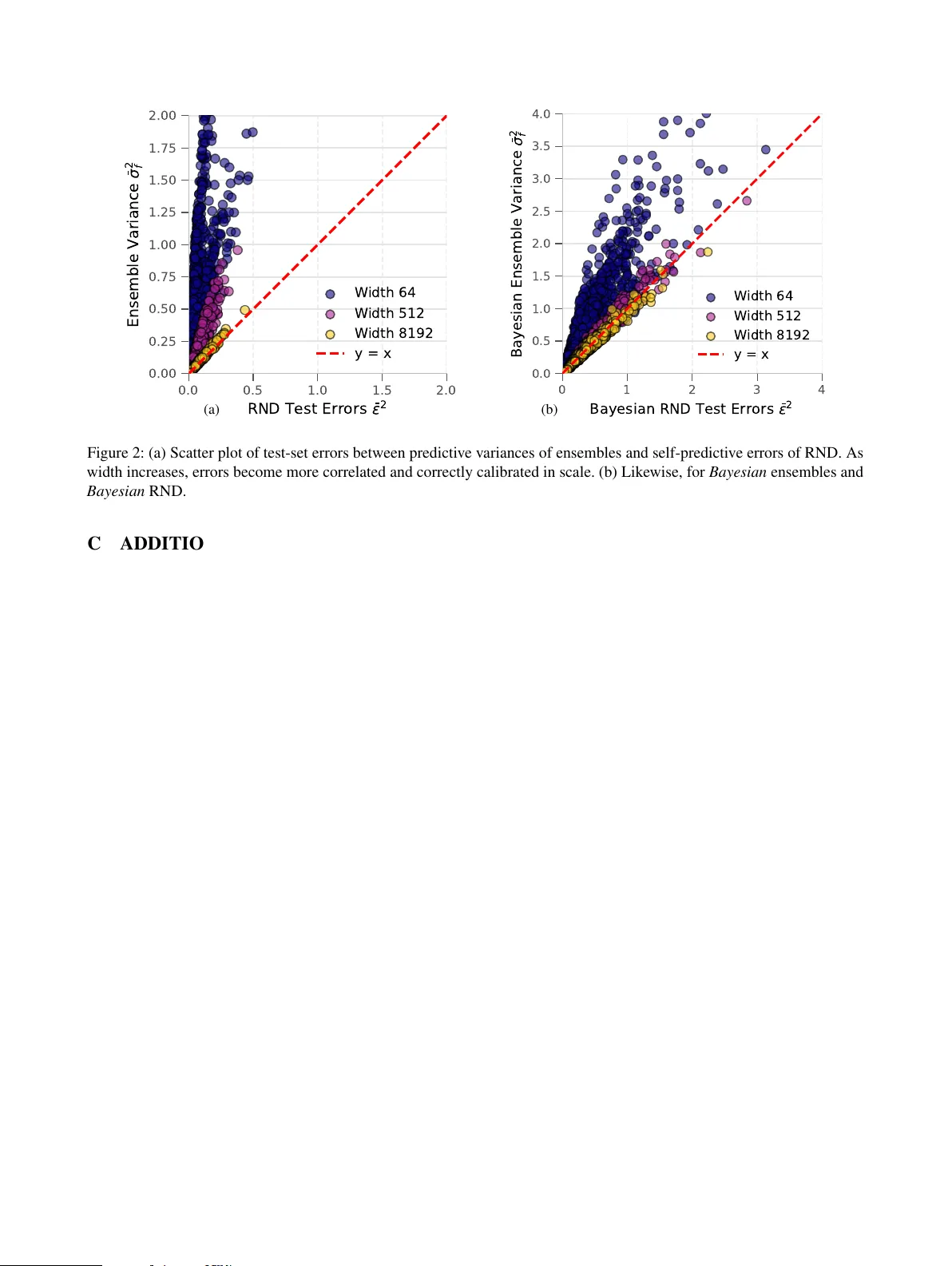
On the Equiv alence of Random Network Distillation, Deep Ensembles, and Bayesian Infer ence Moritz A. Zanger 1 Y ijun W u 1 Pascal R. V an der V aart 1 W endelin Boehmer 1 Matthijs T . J. Spaan 1 1 Delft Univ ersity of T echnology , Delft, 2628 XE, The Netherlands Abstract Uncertainty quantiﬁcation is central to safe and efﬁcient deplo yments of deep learning models, yet many computationally practical methods lack lack- ing rigorous theoretical motiv ation. Random net- work distillation (RND) is a lightweight technique that measures novelty via prediction errors against a ﬁxed random tar get. While empirically effecti ve, it has remained unclear what uncertainties RND measures and ho w its estimates relate to other ap- proaches, e.g., Bayesian inference or deep ensem- bles. W e establish these missing t heoretical connec- tions by analyzing RND within the neural tangent kernel framew ork in the limit of inﬁnite network width. Our analysis rev eals two central ﬁndings in this limit: (1) The uncertainty signal from RND— its squared self-predicti ve error —is equi valent to the predictiv e variance of a deep ensemble. (2) By constructing a speciﬁc RND target function, we show that the RND error distrib ution can be made to mirror the centered posterior predictive distrib u- tion of Bayesian inference with wide neural net- works. Based on this equiv alence, we moreov er de- vise a posterior sampling algorithm that generates i.i.d. samples from an exact Bayesian posterior pre- dictiv e distribution using this modiﬁed Bayesian RND model. Collecti vely , our ﬁndings provide a uniﬁed theoretical perspectiv e that places RND within the principled framew orks of deep ensem- bles and Bayesian inference, and of fer new av enues for efﬁcient yet theoretically grounded uncertainty quantiﬁcation methods. 1 INTR ODUCTION Quantifying predictiv e uncertainty remains a cornerstone of reliable machine learning and underpins applications from safe robotics to ef ﬁciently exploring agents and autonomous scientiﬁc discov ery . Bayesian inference is widely re garded as a theoretical gold-standard to this end [Neal, 1996, Goan and Fook es, 2020] but its application to neural networks is typically intractable in practice, requiring approximations of simpliﬁed posteriors through v ariational inference [VI, Kingma and W elling, 2014, Gal and Ghahramani, 2016, Blei et al., 2017] or complex sampling mechanisms through Markov chain Monte Carlo approaches [MCMC, Chen et al., 2014, Liu and W ang, 2016, Garriga-Alonso and For - tuin, 2021]. Deep ensembles [Dietterich, 2000, Lakshmi- narayanan et al., 2017] on the other hand maintain sev eral independently initialized models to quantify predictive v ari- ance as uncertainty . Due to their simplicity and relativ e practical reliability , deep ensembles ha ve become a widely established alternativ e to Bayesian approaches for uncer- tainty quantiﬁcation in deep learning [Abdar et al., 2021]. Howe ver , both ensemble methods and approximate Bayesian methods typically incur substantial computational and memory costs, in particular for larger-scale models, mo- ti vating more efﬁcient alternatives. RND [Burda et al., 2019] offers one such approach: by training a pr edictor network to mimic the outputs of a ﬁxed, randomly initialized tar get network , RND produces a simple novelty or uncertainty signal via the squared prediction error . Random network distillation (RND) has seen empirical success in e xploration, out-of-distribution detection, and continual learning [Burda et al., 2019, Nikulin et al., 2023, Matthews et al., 2024], yet the theoretical understanding of the nature of its uncertainty estimates remains blurry . In particular , it is unclear ho w—or whether—the RND error relates to the principled uncertain- ties produced for example by Bayesian inference or deep ensembles. In this paper , we establish these missing theoretical con- nections by analyzing random network distillation in the idealized setting of inﬁnite network width. In particular, we establish a Gaussian process (GP) interpretation of the self-predictiv e RND errors in the limit of inﬁnitely wide neural networks, drawing on Neural T angent Kernel (NTK) theory [Jacot et al., 2018, Lee et al., 2020b]. Our three main contributions are: 1. Ensemble equivalence with Standar d RND: W e pro ve that, in the idealized inﬁnite width limit, the squared prediction errors of standard RND coincide exactly with the variance of a deep ensemble. 2. P osterior equivalence with Bayesian RND: By engi- neering the RND target function, we design a Bayesian RND v ariant whose error distrib ution matches that of the exact Bayesian posterior predicti ve distribution of a neural network in the limit of inﬁnite width. 3. P osterior sampling with Bayesian RND: Based on a multi-headed Bayesian RND model, we de vise a pos- terior sampling algorithm that produces i.i.d. samples of the exact Bayesian posterior predicti ve distribution of neural networks in the limit of inﬁnite width. This unifying perspecti ve on the uncertainty estimates pro- duced by RND, deep ensembles, and Bayesian inference provides a no vel understanding and theoretical support for the empirical effecti veness of RND and suggests avenues for future research directions to wards principled Bayesian inference with minimal computational ov erhead. 2 PRELIMINARIES W e begin by establishing notation, deﬁning RND formally , and brieﬂy introducing the theoretical framework used in our analysis. In our analysis, we consider fully connected neural networks f ( x ; θ t ) of L layers of widths n 1 , . . . , n L = n , parametrized by θ t at time t . The forward computation of such networks is deﬁned recursi vely with z l i ( x ; θ ≤ l t ) denot- ing the i -th output of layer l and z l i ( x, θ ≤ l t ) = σ b b l i + σ w √ n l − 1 n l − 1 P j =1 w l ij x l j ( x ) x l j ( x ) = ϕ ( z l − 1 j ( x ; θ ≤ l − 1 t )) , (1) where θ ≤ l t denotes the parameters { w 1 , b 1 , . . . , w l , b l } up to layer l , σ b and σ w denote scaling parameters of the forward computation, and ϕ : R − → R is a Lipschitz- continuous nonlinearity . In Eq. (1) , n 0 = d in and x 1 ( x ) = x . The output of a scalar-output neural network is then giv en by f ( x ; θ t ) = z L ( x ; θ ≤ L t ) . W e furthermore as- sume that parameters are initialized i.i.d. from a normal distribution θ 0 ∼ N (0 , I ) 1 ). For con venience, we will sometimes ov erload notation to concatenate function out- puts, for example indicating a set X = { x i ∈ R d in } N D i =1 and the corresponding function output as a column vec- tor f ( X ; θ t ) = ( f ( x i ; θ t )) N D i =1 , where f ( X ; θ t ) ∈ R N D × K 1 Also known as NTK-parametrization, where variance scalings σ b and σ w affect both forw ard and gradient computations, yielding well-behav ed gradients in the inﬁnite-width limit. or matrix-valued identities Σ( X , X ) = (Σ( x i , x j )) N D i,j =1 , where Σ( X , X ) ∈ R N D × N D . For conciseness our notation will furthermore use a shorthand for cov ariance and kernel matrices denoting Σ X X ≡ Σ( X , X ) . In the following we brieﬂy revie w methods pertinent to this work. Random network distillation. Random network distil- lation [Burda et al., 2019] is an uncertainty quantiﬁcation technique that employs two neural networks of identical architecture: A ﬁxed, randomly initialized target network g ( x ; ψ 0 ) : R d in → R K , and a pr edictor network u ( x ; ϑ t ) , where parameters ϑ t are subject to optimization via gradient descent. The predictor is trained to minimize the expected squared difference to the target netw ork’ s output on a set of data points X = { x i ∈ R d in } N D i =1 L rnd ( ϑ t ) = 1 2 ∥ u ( X ; ϑ t ) − g ( X ; ψ 0 ) ∥ 2 2 . (2) It is common to design RND with a multi headed archi- tecture with output dimension K and individual output heads { u i ( x ; ϑ t ) } K i =1 , and { g i ( x ; ψ 0 ) } K i =1 , where the sum of squared prediction errors ϵ i ( x ; ϑ t , ψ 0 ) = u i ( x ; ϑ t ) − g i ( x ; ψ 0 ) at a test point x serves as an uncertainty signal ϵ 2 ( x ; ϑ t , ψ 0 ) = 1 K K P i =1  u i ( x ; ϑ t ) − g i ( x ; ψ 0 )  2 . (3) Gaussian processes. In our analysis, we will frequently use GPs to model distributions over random functions: A univ ariate GP [Rasmussen and W illiams, 2006] deﬁnes a distribution over functions f 0 ∼ G P ( µ 0 , Σ 0 ) character- ized by a mean function µ 0 : R d in − → R and a cov ariance (kernel) function Σ 0 : R d in × R d in − → R such that f 0 ( X T ) follows a multiv ariate Gaussian distribution f 0 ( X T ) ∼ N ( µ 0 ( X T ) , Σ 0 ( X T , X T )) for any ﬁnite set of ev aluation points X T = { x T est i } N T i =1 . W e can condition a prior GP N ( µ 0 ( X T ) , Σ 0 ( X T , X T )) on training data X = { x i } N D i =1 and labels Y = { y i } N D i =1 to obtain a posterior GP whose posterior pr edictive distrib ution is Gaussian with mean and cov ariance given by µ ( X T ) = µ 0 ( X T ) + Σ 0 X T X (Σ 0 X X ) − 1  Y − µ 0 ( X )  , Σ X T X T = Σ 0 X T X T − Σ 0 X T X (Σ 0 X X ) − 1 Σ 0 X X T . (4) Learning dynamics with inﬁnite width. W e turn to ana- lytical tools to establish solutions to the learning dynamics of neural networks in the limit of inﬁnite width n → ∞ . W ithin this setting, we consider the training dynamics under gradient ﬂow , the continuous-time limit of gradient descent d dt θ t = −∇ θ L ( θ t ) . Under gradient ﬂo w with a square loss L ( θ t ) = 1 2 ∥ f ( X ; θ t ) − Y ∥ 2 2 , the evolution of the NN f is described by a differential equation in function space d d t f ( x ; θ t ) = ∇ θ f ( x ; θ t ) ⊤ d d t θ t = −∇ θ f ( x ; θ t ) ⊤ ∇ θ f ( X ; θ t )( f ( X ; θ t ) − Y ) ≡ − Θ t ( x, X )( f ( X ; θ t ) − Y ) . (5) The above learning dynamics are governed by a gradient similarity function, called the neur al tangent kernel [NTK, Jacot et al., 2018], Θ t ( x, x ′ ) = ∇ θ f ( x ; θ t ) ⊤ ∇ θ f ( x ′ ; θ t ) . While this inner product is dynamic and therefore intractable in general, the limit of inﬁnite network width yields a re- markable simpliﬁcation: 1.) due to large number ef fects, the inner product kernel Θ 0 ( x, x ′ ) at initialization is determin- istic despite the random initialization of θ 0 ; 2.) Θ t ( x, x ′ ) remains constant throughout t under gradient ﬂow [Jacot et al., 2018, Lee et al., 2020b]. In particular, this means lim n →∞ Θ 0 ( x, x ′ ) = lim n →∞ Θ t ( x, x ′ ) ≡ Θ( x, x ′ ) and con verts Eq. 5 into a linear ordinary differential equation, which can be solved analytically . It can be shown that, under mild conditions, f ( x ; θ t ) con verges to the kernel re gression solution [see Jacot et al., 2018, and Appendix B.1] f ( x ; θ ∞ ) = f ( x ; θ 0 ) − Θ x X Θ − 1 X X  Y − f ( X ; θ 0 )  , (6) Moreov er , Lee et al. [2018] show that both f ( x ; θ 0 ) and f ( x ; θ ∞ ) are indeed GPs described by the neural network Gaussian process [NNGP , Lee et al., 2018] f ( x ; θ 0 ) ∼ G P (0 , κ xx ′ ) and the con verged GP deﬁned in Theorem 2.1. Theorem 2.1. [Lee et al., 2020b](Distribution of post- con verg ence neural network functions) Let f ( X T ; θ ∞ ) be a NN as deﬁned in Eq. (1) , and let X T be testpoints. F or r an- dom initializations θ 0 ∼ N (0 , I ) , and in the limit n → ∞ , f ( X T ; θ ∞ ) distributes as a Gaussian with mean and covari- ance given by E [ f ( X T , θ ∞ )] = Θ X T X Θ − 1 X X Y , Σ f X T X T ( θ ∞ ) = κ X T X T + Θ X T X Θ − 1 X X κ X X Θ − 1 X X Θ X X T −  Θ X T X Θ − 1 X X κ X X T + h.c.  , wher e h.c. is the Hermitian conjugate of the pr eceding term. See also Appendix B.1.2 or Lee et al. [2020b]. Note that the GP described in Theorem 2.1 represents the la w by which an inﬁnite ensemble of inﬁnitely wide neural netw orks from i.i.d. initializations distributes after training on ( X , Y ) , but— as is—permits no Bayesian posterior interpretation, which is of the canonical form described in Eq. 4. 3 EQUIV ALENCE OF RANDOM NETWORK DISTILLA TION & DEEP ENSEMBLES W e proceed to characterize formally the relationship be- tween the error signals as measured by random network distillation and the predictive variance of deep neural net- work ensembles. Before treating multiv ariate output dimen- sions in section 3.1, we ﬁrst consider scalar function outputs for simplicity , i.e. f , u, g : R d in − → R with K = 1 . This setup in volves training a predictor u ( x ; ϑ t ) to match a ﬁxed random target function g ( x ; ψ 0 ) . Intuitiv ely , the expected errors ought to v anish for training points in X and remain non-zero elsewhere, inheriting the randomness and gener- alization behaviors of the functions u and g . Owing to the linear training dynamics in the NTK re gime, the dynamics of the error ev olution d d t ϵ ( x ; ϑ t , ψ 0 ) become akin to those outlined in Eq. (5) as d d t ϵ ( x ; ϑ t , ψ 0 ) = ∇ θ u ( x ; ϑ t ) ⊤ d d t ϑ t = −∇ ϑ u ( x ; ϑ t ) ⊤ ∇ ϑ L rnd ( ϑ t ) (7) = − Θ t ( x, X ) ϵ ( x ; ϑ t , ψ 0 ) . W e then draw on the results of Theorem 2.1 to provide a probabilistic description of the self-predicti ve errors ϵ ( x ; ϑ ∞ , ψ 0 ) of a con ver ged RND model in the limit of inﬁnite network width. Theorem 3.1. (Distribution of post-con verg ence RND err ors) Under NTK parametrization, let u ( x ; ϑ ∞ ) be a con ver ged prediction network in t → ∞ , with data X and ﬁxed tar get network g ( X ; ψ 0 ) . Let param- eters ϑ 0 , ψ 0 be drawn i.i.d. ϑ 0 , ψ 0 ∼ N (0 , I ) , with the r esulting NNGP u ( x ; ϑ 0 ) ∼ G P (0 , κ u ( x, x ′ )) and g ( x ; ψ 0 ) ∼ G P (0 , κ g ( x, x ′ )) . The post-con verg ence RND err or ϵ ( X T ; ϑ ∞ , ψ 0 ) is Gaussian with zero mean and co- variance E [ ϵ ( X T , ϑ ∞ , ψ 0 )] = 0 , Σ ϵ X T X T ( ϑ ∞ , ψ 0 ) = κ ϵ X T X T + Θ X T X Θ − 1 X X κ ϵ X X Θ − 1 X X Θ X X T −  Θ X T X Θ − 1 X X κ ϵ X X T + h.c.  , wher e κ ϵ xx ′ = κ u xx ′ + κ g xx ′ is the covariance kernel of ini- tialization err ors ϵ ( x ; ϑ 0 , ψ 0 ) = u ( x ; ϑ 0 ) − g ( x ; ψ 0 ) . Proof sketch. The error function u ( x ; ϑ ∞ ) − g ( x ; ψ 0 ) is a sum of the random post-conv ergence function u ( x ; ϑ ∞ ) and the ﬁxed random target function g ( x ; ψ 0 ) . The latter g ( x ; ψ 0 ) is kno wn to follo w the NNGP . By the linearity of NTK learning dynamics, the online function u ( x ; ϑ ∞ ) is an afﬁne transformation of its initialization u ( x ; ϑ 0 ) , which it- self follows the NNGP . Moreov er , this afﬁne transformation is independent of g or ψ 0 , such that the error ϵ ( x ; ϑ ∞ , ψ 0 ) is a sum of two independent GPs and therefore a GP itself. The resulting GP has zero-mean and covariance with an altered prior NNGP kernel κ ϵ ( x, x ′ ) composed of the online prior kernel κ u xx ′ and the tar get prior kernel κ g xx ′ . See also Appendix B.1.3. Corollary 3.2. (Equivalence in e xpectation between RND err ors and ensemble variance) Under the conditions of Theor em 3.1, let ϵ ( x ; ϑ ∞ , ψ 0 ) be the err or function of a con verg ed RND network with data X . Moreover , for a r e- gr ession pr oblem on X for some labels Y , let V [ f ( x ; θ ∞ )] denote the variance of con verg ed NN functions random ini- tializations. Furthermor e, suppose an arc hitectural equiva- lence between f , u , and g and i.i.d. parameter initialization θ 0 , ϑ 0 , ψ 0 ∼ N (0 , I ) . The expected norm of the RND err or ϵ 2 ( x ; ϑ ∞ , ψ 0 ) then coincides with the ensemble variance E ϑ 0 ,ψ 0  ϵ 2 ( x ; ϑ ∞ , ψ 0 )  = V θ 0 [ f ( x ; θ ∞ )] (8) Proof sketc h. Corollary 3.2 follo ws straighforwardly from Theorem 3.1 by using κ u ( x, x ′ ) = κ g ( x, x ′ ) . T aking the trace of the co variance matrix and di viding by 2 , we reco ver the predictiv e ensemble variance V θ 0 [ f ( x ; θ ∞ )] . Theorem 3.1 and Corollary 3.2 formally show that, for an architectural equi valence between ensemble, predictor and target netw ork, the e xpected RND errors directly quantify the predictiv e variance of the corresponding inﬁnite ensem- ble model described by Theorem 2.1. T o the best of our knowledge, it is the ﬁrst formal analysis of random network distillation in the NTK regime and re veals a ﬁrst theoreti- cal motiv ation for the popular algorithm: in the idealized inﬁnite-width setting, expected RND err ors exactly quantify the variance of deep ensembles for any input x . 3.1 MUL TI-HEADED RANDOM NETWORK DISTILLA TION The analysis thus far has considered the aver age behavior of scalar network outputs for simplicity . While insightful in its own right, this setting does not reﬂect most common prac- tical implementations of random network distillation and instead, if taken literally , would imply an ensemble of ran- dom network distillation models. T o connect with common practical implementations that typically use multi-headed architectures for enhanced reliability and ef ﬁciency , we no w seek to incorporate the probabilistic relation between differ - ent function outputs f i ( x ; θ t ) and f j ( x ′ ; θ t ) of a NN with shared hidden layers in the inﬁnite-width limit. The result below identiﬁes this relationship simply as a statistical in- dependence between the different r andom network outputs f i ( x ; θ t ) and f j ( x ′ ; θ t ) for any time t during gradient ﬂo w optimization. Proposition 3.3. (Independence of NN functions) Under NTK parametrization and in the limit n → ∞ , the ran- dom functions f i ( x ; θ t ) of a NN with K output dimensions and shared hidden layers ar e mutually independent with covariance Σ ij xx ′ ( θ t ) = E [ f i ( x ; θ t ) f j ( x ′ ; θ t )] = ( Σ f xx ′ ( θ t ) i = j , 0 i  = j , on the interval t ∈ [0 , ∞ ) . Proof sketc h. The property follows from known results that state the independence between output dimensions of the NNGP kernel κ and the NTK Θ [Arora et al., 2019, Lee et al., 2018, Jacot et al., 2018]. F or both kernels, the proof proceeds by induction, where the independence property between output dimensions is propagated layer-wise. The induction start is equal for both kernels, where ﬁrst layer outputs, as well as gradients are linear transformations of the Gaussian ﬁrst-layer weights. Both the NNGP and NTK permit a recursiv e formulation, through which the indepen- dence property can be propag ated layer -wise, constituting the induction step. Combined with the learning dynamics of wide NNs, we can conclude that the indi vidual function out- puts of a multi-headed NN, too, are statistically independent for any time t on the interval [0 , ∞ ) . See Appendix B.1.4 or Lee et al. [2018] and Jacot et al. [2018]. Notably , this decoupling holds despite the shared hidden lay- ers and is an artifact of the learning dynamics exhibited in the inﬁnite width limit and the NTK regime. In the absence of feature learning, output functions become statistically independent despite sharing a network body . By virtue of this independence property , a translation of the earlier ob- tained single-function results on RND error distributions (Theorem 3.1 and Corollary 3.2) to the multi-headed set- ting is straightforward. Our ne xt result thus establishes an equiv alence between the errors of the multi-headed RND algorithm, a widely used architecture in practice, and the variance of a ﬁnite-sized deep ensemble. Theorem 3.4. (Distrib utional equivalence between multi- headed RND and ﬁnite deep ensembles) Under the condi- tions of Theorem 3.1, let u i ( x ; ϑ ∞ ) , g i ( x ; ψ 0 ) be the i -th output of pr edictor and targ et networks r espectively with K output dimensions. Denote their sample mean RND er- r or ¯ ϵ 2 ( x ; ϑ ∞ , ψ 0 ) = 1 K P K i =1 ϵ 2 i ( x ; ϑ ∞ , ψ 0 ) . Mor eover , let { f ( x ; θ i ∞ ) } K +1 i =1 be an ensemble of K + 1 NNs fr om i.i.d. ini- tial draws θ 0 . Denote its sample variance ¯ σ 2 f ( x ; θ i...K +1 ∞ ) = 1 K P K +1 i =1 ( f ( x ; θ i ∞ ) − 1 K +1 P K +1 j =1 f ( x ; θ j ∞ )) 2 . The sample mean RND err or and sample ensemble variance distribute to the same law 1 2 ¯ ϵ 2 ( x ; ϑ ∞ , ψ 0 ) D = ¯ σ 2 f ( x ; θ i...K +1 ∞ ) , (9) wher e D = indicates an equality in distribution, namely by a scaled Chi-squared distribution ¯ σ 2 f ( x ; θ i...K +1 ∞ ) ∼ Σ f xx ( θ ∞ ) K χ 2 ( K ) with scale Σ f xx ( θ ∞ ) given by the analytical variance as given in Theor em 2.1. Proof sketch. By Proposition 3.3, the function heads { u i ( x ; ϑ ∞ ) } K i =1 are K independent predictors, each trained to match their independent targets g i ( x ; ψ 0 ) . Thus, the er- rors { ϵ i ( x ; ϑ ∞ , ψ 0 ) } K i =1 are i.i.d. samples from the error distribution outlined in Proposition 3.2. In particular , ¯ ϵ 2 is the empirical mean of i.i.d. samples from a Gaussian which is kno wn to be Chi-squared distrib uted. Similarly , we ha ve that the ensemble { f ( x ; θ i ∞ ) } K +1 i =1 are K + 1 i.i.d. sam- ples from the GP deﬁned in Theorem 2.1, again yielding the kno wn Chi-squared distribution for its sample variance ¯ σ 2 f ( x ; θ i...K +1 ∞ ) . See Appendix B.1.5. Theorem 3.4 establishes a distributional equality between the empirical error of a multi-headed RND architecture and the empirical variance of a ﬁnite ensemble of neural net- works in the limit of inﬁnite width, pro viding a theoretical moti vation for the use of RND and its common multi-headed architecture as an uncertainty quantiﬁcation technique. In a broader sense, we believe this analysis is insightful to many practitioners using random netw ork distillation by establishing an intuitiv e link between theory and practice. Still, the NTK-based perspectiv e applies to an inherently idealized regime and naturally opens up new avenues for in vestigation. Understanding the relationship between RND networks and deep ensembles at ﬁnite width, where feature learning impacts behavior , remains a critical open question beyond the scope of our current framew ork. Y et, intrigu- ing possibilities also arise within the inﬁnite-width setting itself: Could the properties of the RND target network be deliberately chosen or modiﬁed? Exploring different tar get initializations offers a computationally inexpensi ve le ver to shape the uncertainty signal captured by RND. Indeed, pur- suing this very direction, the next section in vestigates ho w a speciﬁc adaptation of the RND tar get function allows us to establish a direct correspondence not just with ensemble variance, but with the principled uncertainty quantiﬁcation provided by Bayesian posterior inference. 4 EQUIV ALENCE OF RANDOM NETWORK DISTILLA TION & B A YESIAN POSTERIORS Having formulated an equiv alence between standard ran- dom network distillation and deep ensemble variance, we now proceed to in vestigate ho w theoretical connections to the Bayesian inference framew ork can be established by in voking deliberate changes to the standard random network distillation algorithm, namely by modifying the ﬁxed target function g . Our goal is to sho w that the RND error signal itself can, under speciﬁc conditions, be interpreted as a draw from a centered Bayesian posterior predictiv e distribution. T o this end, we brieﬂy recall Bayesian inference with the classical Gaussian linear model. W e deﬁne a regres- sion model as f ( x ; θ ) = ϕ ( x ) ⊤ θ with a feature mapping ϕ : R d in − → R d P , and a prior distribution ov er the parame- ters p ( θ ) ∼ N (0 , Σ 0 ) . The prior distrib ution p ( θ ) implicitly deﬁnes a GP prior f 0 ( x ; θ ) ∼ G P (0 , ϕ ( x ) ⊤ Σ 0 ϕ ( x ′ )) , with the prior kernel K xx ′ = ϕ ( x ) ⊤ Σ 0 ϕ ( x ′ ) . W ithin this linear model 2 , we look to infer a posterior distrib ution ov er func- tions given observations X = { x i ∈ R d in } N D i =1 and labels Y = { y i ∈ R } N D i =1 . Owing to our prior choice, the corre- 2 W e use a noise-free regression model for ease of notation here, but e xtensions to the noisy case by including an observation noise term σ 2 n I in the kernel matrix in versions (cf. Eq. (10) - (11) ) are straightforward. sponding posterior pr edictive distribution conditioned on X , Y is a GP with p ( f | x, X , Y ) ∼ N ( K x X K − 1 X X Y , K xx − K x X K − 1 X X K X x ) . (10) When contrasting this identity with the GP governing the distribution of conv erged NN functions of Theorem 3.1, one observes a disparity in the structure of the cov ariance functions. While Theorem 2.1 and Theorem 3.1, too, spec- ify GPs, they do not permit an interpretation as a Bayesian posterior predictiv e distribution [Lee et al., 2020b] due to the presence of two (in general) distinct kernel functions, namely the NNGP kernel κ and the NTK Θ . Howe ver , in- spection of Theorem (3.1) and Eq. (10) suggests a path: if the prior kernel components within Σ ϵ xx ′ ( ϑ ∞ , ψ 0 ) , namely κ ϵ xx ′ , are be aligned with the dynamics kernel Θ xx ′ (i.e., if κ ϵ ∝ Θ ), then the resulting cov ariance structure simpliﬁes to the desired Bayesian posterior form of f ( x ; θ ∞ ) ∼ N  Θ x X Θ − 1 X X Y , Θ xx − Θ x X Θ − 1 X X Θ X x  . (11) An important insight here is that Eq. 11 now is the ex- act Bayesian posterior pr edictive distribution of a neural network in the inﬁnite width limit , which corresponds to a kernel regression model with the NTK as a GP prior G P (0 , Θ xx ′ ) and conditioned on the data ( X , Y ) . The idea of aligning the prior and dynamic kernels has been pre viously explored by He et al. [2020] to construct Bayesian ensembles where the predictive distrib ution of the ensemble matches the posterior predictiv e distribution of the NTK-GP . W e propose that a similar alignment can be achiev ed in the RND framework by constructing the tar get function g ( x ; ψ 0 ) to assume a speciﬁc form. The idea is to design a target ˜ g ( x ; ϑ 0 , ψ 0 ) such that when a predictor u ( x ; ϑ 0 ) is trained to match it, the resulting “Bayesian” error distribution ϵ b ( x ; ϑ ∞ , ϑ 0 , ψ 0 ) = u ( x ; ϑ ∞ ) − ˜ g ( x ; ϑ 0 , ψ 0 ) behav es like a dra w from the posterior of a Bayesian model whose prior kernel is the NTK Θ xx ′ itself 3 . In the random network distillation algorithm, the prior kernel κ ϵ b xx ′ of initialization errors ϵ b ( x ; ϑ 0 , ϑ 0 , ψ 0 ) = u ( x ; ϑ 0 ) − ˜ g ( x ; ϑ 0 , ψ 0 ) is giv en by the sum of the online prior kernel and the tar get prior kernel κ ϵ b xx ′ = κ u xx ′ + κ ˜ g xx ′ (cf. Theorem 3.1), provided that u and ˜ g follo w independent GPs. T o obtain an error prior k ernel that aligns with the NTK such that κ ϵ b xx ′ = Θ xx ′ , one may thus construct the target prior such that it satisﬁes κ ˜ g xx ′ = Θ xx ′ − κ u xx ′ . T o this end, a closer inspection of the relation between the NNGP kernel κ u xx ′ and the NTK Θ xx ′ is instructiv e. For this purpose, we will vie w the online network u ( x ; ϑ 0 ) as a random feature model with its forward computation path as described in 3 The newly constructed tar get function ˜ g ( x ; ϑ 0 , ψ 0 ) uses both ϑ 0 and ψ 0 for reasons that will become clear in the remainder of section. Eq. 1. Let in this scenario x L ( x ) denote the output vector , or the post-activ ations, before the ﬁnal linear layer and denote the last-layer parameters at initialization t = 0 as ( w L , b L ) . W e can write the NN output at initialization u ( x ; ϑ 0 ) as u ( x ; ϑ 0 ) = σ b b L + σ w √ n L − 1 n L − 1 P i =1 w L i x L i ( x ) , (12) that is, as a simple linear model of the random ﬁnal post- activ ations x L ( x ) . V ie wing the function in Eq. (12) as a random feature model leads to a central insight: since the last-layer weights and biases ( w L , b L ) are assumed to be ini- tialized i.i.d. from a standard normal ( w L , b L ) ∼ N (0 , I ) , Eq. (12) describes a (random) afﬁne transformation of a Gaussian vector 4 whose cov ariance in the limit n → ∞ is quantiﬁed by the NNGP kernel κ u xx ′ giv en by κ u xx ′ = E [ u ( x ; ϑ 0 ) u ( x ′ ; ϑ 0 )] = σ 2 b + σ 2 w E [ x L i ( x ) x L i ( x ′ )] . (13) Let us now compare this expression for the the prior kernel κ u xx ′ of the online network with its dynamics kernel Θ xx ′ . In particular , we will split the dynam- ics kernel Θ xx ′ into a last-layer component Θ L xx ′ = ∇ { w L ,b L } u ( x ; ϑ 0 ) ⊤ ∇ { w L ,b L } u ( x ′ ; ϑ 0 ) and a component summarizing all preceding parameters Θ ≤ L − 1 xx ′ = ∇ ϑ ≤ L − 1 u ( x ; ϑ 0 ) ⊤ ∇ ϑ ≤ L − 1 u ( x ′ ; ϑ 0 ) such that Θ xx ′ = Θ L xx ′ + Θ ≤ L − 1 xx ′ . Since u ( x ; ϑ 0 ) is linear in the last-layer parameters { w L , b L } (cf. Eq. 12), we make the crucial ob- servation that the last-layer NTK component Θ L xx ′ equals the NNGP prior kernel Θ L xx ′ = κ u xx ′ 5 . This property gi ves a clear instruction for engineering the prior kernel of the tar- get network: by constructing κ ˜ g xx ′ such that κ ˜ g xx ′ = Θ ≤ L − 1 xx ′ and independently from κ u xx ′ , we obtain an error prior as κ ϵ b xx ′ = κ ˜ g xx ′ + κ u xx ′ = Θ L xx ′ + Θ ≤ L − 1 xx ′ = Θ xx ′ . (14) In the following, we will thus aim to construct a target func- tion ˜ g ( x ; ϑ 0 , ψ 0 ) with the desired property κ ˜ g xx ′ = Θ ≤ L − 1 xx ′ , in particular by modeling ˜ g as a linear function in the feature 4 T o see the correspondence in Eq. 13, ﬁrst notice that due to the i.i.d. initialization of ( w L , b L ) , any cross- products (e.g., inv olving elements indexed with i  = j ) vanish in the expectation E [ u ( x ; ϑ 0 ) u ( x ′ ; ϑ 0 )] . The expecta- tion thus becomes E [ u ( x ; ϑ 0 ) u ( x ′ ; ϑ 0 )] = E w ≤ L ,b ≤ L [ σ 2 b + σ 2 w n L − 1 P n L − 1 i =1 x L i ( x ) x L i ( x ′ )] . By linearity , the expectation on the r .h.s. can be pulled inside the sum and by symmetry we hav e that E w ≤ L ,b ≤ L [ x L i ( x ) x L i ( x ′ )] is independent of i , s.t. E w ≤ L ,b ≤ L [ σ 2 w n L − 1 P n L − 1 i =1 x L i ( x ) x L i ( x ′ )] = σ 2 w E [ x L i ( x ) x L i ( x ′ )] . 5 T o see this correspondence, notice that the last-layer gradient inner product ∇ { w L ,b L } u ( x ; ϑ 0 ) ⊤ ∇ { w L ,b L } u ( x ′ ; ϑ 0 ) reduces to the sum σ 2 b + σ 2 w n L − 1 P n L − 1 i =1 x L i ( x ) x L i ( x ′ ) , where the r .h.s. sum tends to its expectation in the limit n L − 1 → ∞ giv en that sum- mands are identically distributed (as before by symmetry) and independent (which is shown more rigorously for example in Sec. B.1.4). space corresponding to gradients in earlier layers. This ap- proach has also previously been e xplored by He et al. [2020] to obtain Bayesian ensembles. Proposition 4.1. (Bayesian RND tar get function) Under the conditions of Theorem 3.1, let u ( x ; ϑ 0 ) and g ( x ; ψ 0 ) be neural networks of L layers with parameters ϑ 0 , ψ 0 ∼ N (0 , I ) i.i.d. Mor eover , let ψ L 0 = { w L , b L } denote the last- layer parameters of ψ 0 and ψ ≤ L − 1 0 the parameters of all pr eceding layers. Suppose the tar get function ˜ g ( x ; ϑ 0 , ψ 0 ) is given by ˜ g ( x ; ϑ 0 , ψ 0 ) = ∇ ϑ 0 u ( x ; ϑ 0 ) ⊤ ψ ∗ 0 , wher e ψ ∗ 0 = { ψ ≤ L − 1 0 , 0 dim ( ψ L 0 ) } is a copy of ψ 0 with its last-layer weights set to 0 . In the inﬁnite width limit n → ∞ , ˜ g ( x ; ϑ 0 , ψ 0 ) distributes by construction as ˜ g ( x ; ϑ 0 , ψ 0 ) ∼ G P (0 , κ ˜ g xx ′ ) wher e κ ˜ g xx ′ = Θ ≤ L − 1 xx ′ . Proof sketc h. The function ˜ g ( x ; ϑ 0 , ψ 0 ) is by construction equiv alent to a linear function with the (random) feature map ∇ ϑ ≤ L − 1 0 u ( x ; ϑ 0 ) giv en by the gradient of parameters in the pre-ﬁnal layers and with a parameter vector ψ ≤ L − 1 0 . Conditioned on ϑ 0 , the random function ˜ g ( x ; ϑ 0 , ψ 0 ) is thus an afﬁne transformation of the Gaussian vector ψ ≤ L − 1 0 and thus a GP itself, at any width n . Using the central results by Jacot et al. [2018] that Θ 0 ,xx ′ → Θ xx ′ as n → ∞ and appealing to the bounded con vergence theorem, the limiting distribution of the unconditioned random function ˜ g ( x ; ϑ 0 , ψ 0 ) , too, becomes Gaussian with the deterministic cov ariance Θ ≤ L − 1 xx ′ . While the speciﬁc form of the kernel Θ ≤ L − 1 xx ′ = Θ xx ′ − Θ L xx ′ seems unusual as a standalone prior , it is crucially impor - tant in shaping the ﬁnal error distribution. This is because with the altered “Bayesian” target function ˜ g ( x ; ϑ 0 , ψ 0 ) we can shape the cov ariance structure of errors at initialization by satisfying Eq. 14, appealing to Theorem (3.1) . W ith the engineered tar get function ˜ g ( x ; ϑ 0 , ψ 0 ) , the learning dynam- ics of an RND model where the predictor network u ( x ; ϑ t ) learns to mimic ˜ g ( X ; ϑ 0 , ψ 0 ) can be shaped in the desired way . Our central statement is that the distribution of the error between the conv erged predictor u ( x ; ϑ ∞ ) and the target function ˜ g ( x ; ϑ 0 , ψ 0 ) will then no longer reﬂect the variance of deep ensembles trained with gradient descent, but will instead directly exhibit the statistics of a Bayesian posterior predicti ve distrib ution deri ved from the NTK-GP prior . Theorem 4.2 formalizes this result. Theorem 4.2. (Distrib ution of Bayesian RND err ors) Un- der the conditions of Theor em 3.1, let u ( x ; ϑ ∞ ) be a con verg ed predictor network trained on data X with la- bels fr om the ﬁxed tar get function ˜ g ( X ; ϑ 0 , ψ 0 ) as deﬁned in Pr oposition 4.1. Let parameters ϑ 0 , ψ 0 be drawn i.i.d. ϑ 0 , ψ 0 ∼ N (0 , I ) . The con verg enced Bayesian RND err or ϵ b ( X T ; ϑ ∞ , ϑ 0 , ψ 0 ) = u ( X T ; ϑ ∞ ) − ˜ g ( X T ; ϑ 0 , ψ 0 ) on a test set X T is Gaussian with zer o mean and covariance Σ ϵ b X T X T ( ϑ ∞ , ϑ 0 , ψ 0 ) = Θ X T X T − Θ X T X Θ − 1 X X Θ X X T , and thus recover s the covariance of the exact Bayesian posterior pr edictive distribution of an inﬁnitely wide neural network with the corr esponding NTK Θ xx ′ . Proof sketc h. The result follo ws by combining Theorem 3.1 and Proposition 4.1, provided that the GP gov erning the predictor initialization κ u xx ′ and the target function κ ˜ g xx ′ are independent. Owing to the fact that the parameters ϑ 0 and ψ 0 are drawn independently , the independence between u ( x ; ϑ 0 ) and ˜ g ( x ; ϑ 0 , ψ 0 ) is apparent by rewriting the co- v ariance E [ u ( x ; ϑ 0 ) ˜ g ( x ; ϑ 0 , ψ 0 )] in terms of conditional ex- pectations on ϑ 0 by the law of total expectation. Further- more, since Θ xx ′ = Θ L xx ′ + Θ ≤ L − 1 xx ′ and κ ˜ g xx ′ = Θ ≤ L − 1 xx ′ , κ u xx ′ = Θ L xx ′ , we hav e that κ ϵ b xx ′ = Θ xx ′ . In other words, the GP kernel of initial errors aligns with the NTK of the on- line predictor , such that the distribution of post-con ver gence errors in Theorem 3.1 simpliﬁes signiﬁcantly . This same cov ariance function indeed also deﬁnes the posterior pre- dictiv e distribution of inﬁnitely wide neural networks as de- scribed by the GP with prior G P (0 , Θ xx ′ ) and conditioned on ( X , Y ) . Theorem 4.2 sho ws that with a speciﬁcally engineered tar- get function, the RND error signal ϵ b ( x ; ϑ ∞ , ϑ 0 , ψ 0 ) = u ( x ; ϑ ∞ ) − ˜ g ( x ; ϑ 0 , ψ 0 ) is no longer just related to en- semble variance, but rather becomes a direct sample from the centered posterior predicti ve distrib ution of a Bayesian model whose prior kernel is the NTK itself. This nov el re- sult provides a direct bridge between RND and Bayesian inference in the limit of inﬁnite network width, providing a useful insight: the error signal generated by this mod- iﬁed RND procedure is not merely a heuristic measure of distance, but is itself a random draw from the (cen- tered) Bayesian posterior predictiv e distribution of an NTK- based GP . This direct distributional equi valence has imme- diate practical implications, for example prescribing rather straightforwardly ho w this Bayesian form of RND can be used for exact posterior sampling. By applying Proposi- tion 3.3 to the multi-headed Bayesian RND architecture 6 , in contrast to obtaining samples from deep ensembles as done in Theorem 3.4, we no w obtain sev eral independent samples from the centered posterior predicti ve distribution through ϵ b i ( x ; ϑ ∞ , ϑ 0 , ψ 0 ) = u i ( x ; ϑ ∞ ) − ˜ g i ( x ; ϑ 0 , ψ 0 ) . The belo w corollary details ho w this can be le veraged to conduct a pos- terior sampling procedure, requiring access only to a mean estimate and a single Bayesian RND model. Corollary 4.3 (Posterior Sampling via Bayesian RND) . Let N  µ b ( x ) , Σ b xx ′  be the posterior predictive distribution 6 In a multi-headed architecture, the Bayesian target function described in Proposition 4.2 becomes a JVP . Several common machine learning libraries (e.g., J AX [Bradbury et al., 2018] offer dedicated algorithms to compute such JVPs efﬁciently . of an inﬁnitely wide neur al network conditioned on x with mean µ b ( x ) = Θ x X Θ − 1 X X Y and covariance Σ b xx ′ = Θ xx ′ − Θ x X Θ − 1 X X Θ X x ′ . Suppose ˜ µ ( x ; θ ∞ ) ≈ µ b ( x ) is an estimate of the mean function and let { ϵ b i ( x ; ϑ ∞ , ϑ 0 , ψ 0 ) } K i =1 be er- r or functions of a K -head Bayesian RND model as deﬁned in Theor em 4.2. The following pr ocedur e generates (at most K ) independent samples fr om the conditional posterior pr edictive distribu- tion N  µ b ( x ) , Σ b xx ′  : 1. sample i ∼ U [1 , K ] 2. compute ˜ µ i ( x ) = ˜ µ ( x ; θ ∞ ) + ϵ b i ( x ; ϑ ∞ , ϑ 0 , ψ 0 ) 3. ˜ µ i ( x ) is an i.i.d. sample fr om the conditional posterior pr edictive N  µ b ( x ) , Σ b xx ′  Proof sketch. The result follows directly from Theorem (4.2) and application of the independence argument of Proposi- tion (3.3) to the multi-headed setting. Corollary 4.3 sho ws that, gi ven an estimator of the posterior predictiv e mean, a modiﬁed Bayesian RND setup can be used to perform direct Bayesian posterior sampling in the NTK limit. By extension, this of fers a pathway to perform- ing exact Bayesian inference through the lens of network distillation, provided that the tar get and predictor networks initializations are handled deliberately . This completes our theoretical de velopment, ﬁrst sho wing an equivalence of RND in the NTK regime to ensemble v ariance and no w , through speciﬁc modiﬁcations to its target function, to the generation of independent samples from exact Bayesian posterior predicti ve distributions. 5 NUMERICAL ANAL YSIS W e proceed with a numerical analysis to v alidate the thus far presented results. In the following, we study how predicti ve RND errors relate to predictive v ariances of deep ensem- bles in practice, both in the standard and Bayesian settings. T o this end, we train two-layer connected neural netw orks with SiLU acti v ations [Elfwing et al., 2018] on a synthetic dataset with N = 10 train and ˜ N = 5000 test samples from an isotropic Gaussian x i ∼ N (0 , I 3 ) . Ensemble models are ﬁt to a toy target function, and multiheaded RND models optimized as described abo ve. The v ariance of the true un- derlying GP is approximated with Monte-Carlo estimates of 512 independent models and a single Bayesian RND model with 512 heads, such that a small residual amount of dis- crepancy is to be expected. Fig. 1 shows a stark decrease in av erage squared discrepancy between test ev aluations of predictiv e ensemble variances and RND errors as model width increases, a trend in line with our theoretical deriv a- tions and present e ven at practical netw ork widths. Further ev aluations and details of this experiment are reported in Appendix C. 64 128 256 512 1024 2048 4096 8192 L a y e r W i d t h n 0.00 0.02 0.04 0.06 0.08 0.10 0.12 Square Error (Ens. V ar . - RND Err .) S t a n d a r d E n s . - R N D : ( 1 2 2 2 f ) 2 B a y e s . E n s . - B a y e s . R N D : ( 2 2 f ) 2 Figure 1: T est-set errors between predictiv e variances of (Bayesian) ensembles and self-predictiv e errors of (Bayesian) RND vanish with lar ge layer widths. 6 RELA TED WORK A substantial body of research studies the analytical learning dynamics of deep learning, particularly in the inﬁnite-width limit. Central to our analysis are seminal works charac- terizing the NNGP [Lee et al., 2018] at initialization, the dynamics-gov erning NTK [Jacot et al., 2018], and the e vo- lution of wide networks as linear models [Lee et al., 2020b, Arora et al., 2019, Chizat and Bach, 2018]. This provides a theoretical frame work for analytical descriptions of deep en- sembles [Lakshminarayanan et al., 2017, Dietterich, 2000], with subsequent studies using NTK theory to precisely char - acterize ensemble variances under v arious conditions, in- cluding observation noise [Y ang, 2019, K obayashi et al., 2022, Calvo-Ordoñez et al., 2024]. A central line of work for our paper is the connection between deep ensembles and Bayesian inference in inﬁnite-width NTK regime. Notably , He et al. [2020] demonstrate how to construct “Bayesian ensembles”, an approach we adopt to construct “Bayesian RND” algorithms. The broader link between deep ensem- bles and approximations of Bayesian posteriors has been studied extensi vely [Khan et al., 2019, Osawa et al., 2019, D’Angelo and Fortuin, 2021, Osband et al., 2019, Izmailov et al., 2021]. More recently , NTK-based approaches have been used for single-model uncertainty estimation [Zanger et al., 2026a] or ad-hoc uncertainty quantiﬁcation [W ilson et al., 2025]. Our work pro vides a theoretical basis for RND [Burda et al., 2019], which belongs to a class of computa- tionally cheaper , single-model methods [Pathak et al., 2017, Lahlou et al., 2021, Guo et al., 2022, Sensoy et al., 2018, V an Amersfoort et al., 2020, Rudner et al., 2022, Laurent et al., 2022, T agasovska and Lopez-P az, 2019]. Moreover , Uncertainty quantiﬁcation from the lens of learning dy- namics is moreov er widespread in reinforcement learning (RL)[Xiao et al., 2021, Cai et al., 2019, W ai et al., 2020, L yle et al., 2022, Y ang et al., 2020], the original application domain of RND. Notably , Zanger et al. [2026b] deri ve an RND-like estimator for v alue function uncertainty using NTK theory . More broadly , deep ensembles and Bayesian methods are widely used in RL, driving exploration [Osband et al., 2016, Chen et al., 2017, Osband et al., 2019, Nikolov et al., 2019, Ishfaq et al., 2021, Zanger et al., 2024]. 7 CONCLUSIONS In this work, we hav e established a novel theoretical un- derstanding of random network distillation (RND) by con- necting it to the principled uncertainty frame works of deep ensembles and Bayesian inference. By analyzing these tech- niques within the unifying setting of inﬁnitely wide neural networks, we pro vide a clear analytical interpretation for the empirically successful RND algorithm. Our analysis yields a twofold equi v alence: ﬁrst, we prove that the squared error of standard RND exactly recov ers the predictiv e v ariance of deep ensembles in the NTK regime. Second, we demonstrate that the RND frame work is more v ersatile; by deliberately designing the RND tar get function, the resulting error sig- nal can be made to directly mirror the centered posterior predictiv e distribution of an NTK-gov erned GP , that is, the exact posterior predictiv e distribution of neural networks in the inﬁnite width limit. This “Bayesian RND” variant furthermore allo ws for posterior sampling procedures that produce i.i.d. samples from this posterior . Our work thereby uniﬁes RND, ensembles, and Bayesian inference under the same theoretical lens from an inﬁnite width perspectiv e. Crucially , our ﬁndings hold under the assumptions inﬁnite- width and the NTK regime, a setting where networks ef- fectiv ely linearize and operate as kernel machines with a ﬁxed kernel. This “lazy” training re gime, while analytically tractable and predictiv e for very wide networks, does not capture the phenomenon of feature learning. The degree to which our established equiv alences translate to practical, ﬁnite-width networks that learn features remains a signiﬁ- cant open question. Con versely , this also suggest av enues for future research: de viations between RND, ensembles, and Bayesian posteriors in practice must arise from departures from the NTK regime. Characterizing speciﬁcally these deviations could lead to novel techniques and a deeper un- derstanding of computationally efﬁcient approaches that approximate Bayesian inference, operating well outside the kernelized inﬁnite-width setting. Another exciting direction is the concept of tar get engineering as cheap way of study- ing priors for Bayesian deep learning, an activ ely studied ﬁeld that garners widespread interested from the uncertainty quantiﬁcation and Bayesian deep learning community . References Moloud Abdar, Farhad Pourpanah, Sadiq Hussain, Dana Rezazadegan, Li Liu, Mohammad Ghav amzadeh, Paul Fieguth, Xiaochun Cao, Abbas Khosravi, U. Rajen- dra Acharya, Vladimir Makarenkov , and Saeid Na- hav andi. A revie w of uncertainty quantiﬁcation in deep learning: T echniques, applications and challenges. arXiv:2011.06225 , 2021. Sanjeev Arora, Simon S Du, W ei Hu, Zhiyuan Li, Russ R Salakhutdinov , and Ruosong W ang. On exact compu- tation with an inﬁnitely wide neural net. Advances in neural information pr ocessing systems , 32, 2019. David M Blei, Alp K ucukelbir , and Jon D McAuliffe. V ari- ational inference: A revie w for statisticians. Journal of the American statistical association , 112(518):859–877, 2017. James Bradb ury , Ro y Frostig, Peter Ha wkins, Matthew James Johnson, Chris Leary , Dougal Maclaurin, George Necula, Adam Paszke, Jake V anderPlas, Skye W anderman-Milne, and Qiao Zhang. J AX: composable transformations of Python+NumPy programs, 2018. URL http://github.com/jax- ml/jax . Y uri Burda, Harrison Edwards, Amos J. Storke y , and Ole g Klimov . Exploration by random network distillation. In International confer ence on learning repr esentations , 2019. Qi Cai, Zhuoran Y ang, Jason D Lee, and Zhaoran W ang. Neural temporal-diff erence learning con verges to global optima. Advances in neural information pr ocessing sys- tems , 32, 2019. Sergio Calvo-Ordoñez, K onstantina Palla, and Kamil Ciosek. Epistemic uncertainty and observation noise with the neural tangent kernel. arXiv pr eprint arXiv:2409.03953 , 2024. Y uan Cao and Quanquan Gu. Generalization bounds of stochastic gradient descent for wide and deep neural net- works. Advances in neural information processing sys- tems , 32, 2019. Richard Y Chen, Szymon Sidor, Pieter Abbeel, and John Schulman. UCB exploration via Q-ensembles. arXiv pr eprint arXiv:1706.01502 , 2017. T ianqi Chen, Emily Fox, and Carlos Guestrin. Stochastic gradient hamiltonian monte carlo. In International con- fer ence on machine learning , pages 1683–1691. PMLR, 2014. Lenaic Chizat and Francis Bach. On the global conv ergence of gradient descent for over -parameterized models us- ing optimal transport. Advances in neural information pr ocessing systems , 31, 2018. Francesco D’Angelo and V incent Fortuin. Repulsive deep ensembles are bayesian. Advances in Neural Information Pr ocessing Systems , 34:3451–3465, 2021. Thomas G Dietterich. Ensemble methods in machine learn- ing. In Multiple classiﬁer systems: F irst international workshop, MCS . Springer , 2000. Rick Durrett. Pr obability: Theory and e xamples , volume 49. Cambridge univ ersity press, 2019. Stefan Elfwing, Eiji Uchibe, and Kenji Doya. Sigmoid- weighted linear units for neural network function approx- imation in reinforcement learning. Neural networks , 107: 3–11, 2018. Y arin Gal and Zoubin Ghahramani. Dropout as a Bayesian approximation: Representing model uncertainty in deep learning. In International confer ence on machine learn- ing , pages 1050–1059. PMLR, 2016. Adrià Garriga-Alonso and V incent Fortuin. Exact langevin dynamics with stochastic gradients. arXiv preprint arXiv:2102.01691 , 2021. Ethan Goan and Clinton Fookes. Bayesian neural networks: An introduction and survey . Case studies in applied Bayesian data science: CIRM Jean-Morlet chair , F all 2018 , pages 45–87, 2020. Zhaohan Guo, Shantanu Thakoor , Miruna Pîslar , Bernardo A vila Pires, Florent Altché, Corentin T allec, Alaa Saade, Daniele Calandriello, Jean-Bastien Grill, Y unhao T ang, et al. BYOL-Explore: Exploration by bootstrapped predic- tion. Advances in neural information pr ocessing systems , 35:31855–31870, 2022. Bobby He, Balaji Lakshminarayanan, and Y ee Whye T eh. Bayesian deep ensembles via the neural tangent kernel. Advances in neural information pr ocessing systems , 33, 2020. Haque Ishfaq, Qiwen Cui, V iet Nguyen, Alex A youb, Zhuoran Y ang, Zhaoran W ang, Doina Precup, and Lin Y ang. Randomized exploration in reinforcement learning with general value function approximation. In Interna- tional confer ence on machine learning , pages 4607–4616. PMLR, 2021. Pa vel Izmailov , Sharad V ikram, Matthew D Hof fman, and Andrew Gordon Gordon W ilson. What are Bayesian neu- ral network posteriors really lik e? In International con- fer ence on machine learning , pages 4629–4640. PMLR, 2021. Arthur Jacot, Franck Gabriel, and Clément Hongler . Neural tangent kernel: Con vergence and generalization in neural networks. Advances in neural information pr ocessing systems , 31, 2018. Mohammad Emtiyaz Khan, Alexander Immer , Ehsan Abedi, and Maciej K orzepa. Approximate inference turns deep networks into gaussian processes. Advances in neural information pr ocessing systems , 32, 2019. Diederik P . Kingma and Max W elling. Auto-encoding vari- ational Bayes. In Y oshua Bengio and Y ann LeCun, ed- itors, International conference on learning repr esenta- tions , 2014. Seijin Kobayashi, Pau V ilimelis Aceituno, and Johannes V on Oswald. Disentangling the predictiv e variance of deep ensembles through the neural tangent kernel. Ad- vances in Neural Information Pr ocessing Systems , 35: 25335–25348, 2022. Salem Lahlou, Moksh Jain, Hadi Nekoei, V ictor Ion Butoi, Paul Bertin, Jarrid Rector-Brooks, Maksym K orablyov , and Y oshua Bengio. Deup: Direct epistemic uncertainty prediction. arXiv preprint , 2021. Balaji Lakshminarayanan, Alexander Pritzel, and Charles Blundell. Simple and scalable predicti ve uncertainty esti- mation using deep ensembles. Advances in neural infor- mation pr ocessing systems , 30, 2017. Olivier Laurent, Adrien Laf age, Enzo T artaglione, Geof frey Daniel, Jean-Marc Martinez, Andrei Bursuc, and Gianni Franchi. Packed-ensembles for efﬁcient uncertainty esti- mation. arXiv preprint , 2022. Jaehoon Lee, Jascha Sohl-dickstein, Jef frey Pennington, Ro- man Nov ak, Sam Schoenholz, and Y asaman Bahri. Deep neural networks as Gaussian processes. In International confer ence on learning repr esentations , 2018. Jaehoon Lee, Samuel Schoenholz, Jeffre y Pennington, Ben Adlam, Lechao Xiao, Roman Nov ak, and Jascha Sohl- Dickstein. Finite versus inﬁnite neural networks: an em- pirical study . Advances in Neural Information Pr ocessing Systems , 33:15156–15172, 2020a. Jaehoon Lee, Lechao Xiao, Samuel S. Schoenholz, Y asaman Bahri, Roman Nov ak, Jascha Sohl-Dickstein, and Jeffre y Pennington. W ide Neural Networks of Any Depth Evolve as Linear Models Under Gradient Descent. Journal of Statistical Mechanics: Theory and Experiment , 2020, De- cember 2020b. Qiang Liu and Dilin W ang. Stein variational gradient de- scent: A general purpose Bayesian inference algorithm. Advances in neural information pr ocessing systems , 29, 2016. Clare L yle, Mark Rowland, Will Dabne y , Marta Kwiatko wska, and Y arin Gal. Learning dynamics and generalization in reinforcement learning. arXiv pr eprint arXiv:2206.02126 , 2022. Michael Matthe ws, Michael Beukman, Benjamin Ellis, Mikayel Samvelyan, Matthe w Jackson, Samuel Coward, and Jakob Foerster . Craftax: A lightning-fast benchmark for open-ended reinforcement learning. arXiv pr eprint arXiv:2402.16801 , 2024. Radford M Neal. Bayesian Learning for Neural Networks . Springer-V erlag, 1996. Nikolay Nikolo v , Johannes Kirschner , Felix Berkenkamp, and Andreas Krause. Information-directed exploration for deep reinforcement learning. In International conference on learning r epresentations, ICLR , 2019. Alexander Nikulin, Vladisla v Kurenko v , Denis T arasov , and Serge y K olesnikov . Anti-exploration by random network distillation. In International Confer ence on Machine Learning , pages 26228–26244. PMLR, 2023. Atsushi Nitanda and T aiji Suzuki. Optimal rates for av- eraged stochastic gradient descent under neural tangent kernel regime. In International confer ence on learning r epresentations , 2021. Kazuki Osawa, Siddharth Swaroop, Mohammad Emtiyaz Khan, Anirudh Jain, Runa Eschenhagen, Richard E T urner, and Rio Y okota. Practical deep learning with bayesian principles. Advances in neural information pr o- cessing systems , 32, 2019. Ian Osband, Charles Blundell, Alexander Pritzel, and Ben- jamin V an Roy . Deep exploration via bootstrapped DQN. Advances in neural information pr ocessing systems , 29, 2016. Ian Osband, Benjamin V an Roy , Daniel J Russo, Zheng W en, et al. Deep exploration via randomized value functions. Journal of mac hine learning resear ch , 20, 2019. Deepak P athak, Pulkit Agrawal, Alexei A. Efros, and T re vor Darrell. Curiosity-driven e xploration by self-supervised prediction. In International confer ence on machine learn- ing . PMLR, 2017. C. E. Rasmussen and C. K. I. W illiams. Gaussian pr ocesses for machine learning . MIT Press, 2006. T im GJ Rudner, Zonghao Chen, Y ee Whye T eh, and Y arin Gal. T ractable function-space variational inference in bayesian neural networks. Advances in neural informa- tion pr ocessing systems , 35:22686–22698, 2022. Maxim Samarin, V olker Roth, and Da vid Belius. On the em- pirical neural tangent kernel of standard ﬁnite-width con- volutional neural network architectures. arXiv preprint arXiv:2006.13645 , 2020. Mariia Seleznov a and Gitta Kutyniok. Analyzing ﬁnite neu- ral networks: Can we trust neural tangent k ernel theory? In Mathematical and Scientiﬁc Machine Learning , pages 868–895. PMLR, 2022. Murat Sensoy , Lance Kaplan, and Melih Kandemir . Eviden- tial deep learning to quantify classiﬁcation uncertainty . Advances in neural information pr ocessing systems , 31, 2018. Natasa T agaso vska and David Lopez-Paz. Single-model uncertainties for deep learning. Advances in neural infor- mation pr ocessing systems , 32, 2019. Joost V an Amersfoort, Lewis Smith, Y ee Whye T eh, and Y arin Gal. Uncertainty estimation using a single deep deterministic neural network. In International conference on machine learning , pages 9690–9700. PMLR, 2020. Hoi-T o W ai, Zhuoran Y ang, Zhaoran W ang, and Mingyi Hong. Prov ably efﬁcient neural GTD for off-polic y learn- ing. Advances in Neural Information Pr ocessing Systems , 33:10431–10442, 2020. Joseph Wilson, Chris v an der Heide, Liam Hodgkin- son, and Fred Roosta. Uncertainty quantiﬁcation with the empirical neural tangent kernel. arXiv preprint arXiv:2502.02870 , 2025. Chenjun Xiao, Bo Dai, Jincheng Mei, Oscar A Ramirez, Ramki Gummadi, Chris Harris, and Dale Schuurmans. Understanding and leveraging overparameterization in recursiv e value estimation. In International Conference on Learning Repr esentations , 2021. Greg Y ang. Scaling limits of wide neural networks with weight sharing: Gaussian process behavior , gradient in- dependence, and neural tangent kernel deri vation. arXiv pr eprint arXiv:1902.04760 , 2019. Zhuoran Y ang, Chi Jin, Zhaoran W ang, Mengdi W ang, and Michael Jordan. Prov ably ef ﬁcient reinforcement learn- ing with kernel and neural function approximations. Ad- vances in Neural Information Pr ocessing Systems , 33: 13903–13916, 2020. Moritz Akiya Zanger , W endelin Böhmer , and Matthijs T J Spaan. Diverse projection ensembles for distributional reinforcement learning. In International confer ence on learning r epresentations , 2024. Moritz Akiya Zanger, Pascal R. V an der V aart, W endelin Boehmer , and Matthijs T . J. Spaan. Contextual similarity distillation: Ensemble uncertainties with a single model. In International confer ence on learning repr esentations , 2026a. Moritz Akiya Zanger , Max W eltevrede, Y aniv Oren, P ascal R. V an der V aart, Caroline Horsch, W endelin Boehmer , and Matthijs T . J. Spaan. Uni versal v alue-function uncer- tainties. In International confer ence on learning r epre- sentations , 2026b. On the Equiv alence of Random Network Distillation, Deep Ensembles, and Bayesian Infer ence (Supplementary Material) Moritz A. Zanger 1 Y ijun W u 1 Pascal R. V an der V aart 1 W endelin Boehmer 1 Matthijs T . J. Spaan 1 1 Delft Univ ersity of T echnology , Delft, 2628 XE, The Netherlands A LIMIT A TIONS AND ASSUMPTIONS W e provide an ov erview of the primary assumptions underpinning our analysis and discuss their relation to practical sett ings. The foremost assumption is that our analysis operates within the NTK regime. This frame work presupposes the asymptotic limit of inﬁnitely wide neural networks and a so-called NTK-parametrization of forward computations that ensures network dynamics linearize around their initialization, leading to “lazy” learning with kernel regression behavior . This idealized setting naturally deviates from practical implementations in volving ﬁnite-width networks. Nonetheless, a signiﬁcant body of work has demonstrated that predictions from NTK theory can remain remarkably accurate for sufﬁciently wide, modern architectures, providing a reasonable approximation of their behavior [e.g., Lee et al., 2020a, Seleznov a and Kutyniok, 2022, Samarin et al., 2020]. Furthermore, our deri v ations assume training via full-batch gradient ﬂo w , which corresponds to gradient descent with an inﬁnitesimal step size. This abstains from the use of stochastic minibatch optimizers, which are standard in practice. While beyond our current scope, e xtensions of NTK analysis to incorporate the effects of stochastic gradient noise do exist [e.g., Y ang, 2019, Cao and Gu, 2019, Nitanda and Suzuki, 2021]. Finally , our analysis considers a ﬁxed training dataset X . This contrasts with prominent applications of RND, particularly in online reinforcement learning, where the agent interacts with an en vironment and learns from an inherently non-stationary data stream. Characterizing ho w these equi valences with ensembles and Bayesian posteriors ev olve under such distribution shifts remains an important open question. B PR OOFS This section provides e xtended proofs for our analysis of RND. B.1 ENSEMBLE EQUIV ALENCE Our ﬁrst result states the equiv alence of self-predictiv e errors of RND and predictiv e variance of deep ensembles in the inﬁnite-width NTK regime. F or completeness, we also include proofs or simpliﬁed proof sketches for kno wn results that support our analysis. Theorem B.1. [J acot et al., 2018](P ost-conver gence neural network function) In the limit of inﬁnite layer widths n − → ∞ and inﬁnite time t − → ∞ , the output function of a neural network f ( x ; θ ∞ ) with NTK parametrization accor ding to Eq. 1 is given by f ( x ; θ ∞ ) = f ( x ; θ 0 ) − Θ x X Θ − 1 X X  Y − f ( X ; θ 0 )  , wher e we used the shorthand Θ xx ′ ≡ Θ( x, x ′ ) . Proof sketch. By taking the inﬁnite width limit n → ∞ , we obtain a linear ODE from Eq. (5) . Through an exponential ansatz, its explicit solution with initial condition f ( x ; θ 0 ) is giv en by f ( x ; θ t ) = f ( x ; θ 0 ) + Θ x X Θ − 1 X X ( I − e − t Θ X X )( Y − f ( X ; θ 0 )) . Assuming the training Gram matrix Θ X X is positi ve deﬁnite (and thus in vertible), the exponential term decays to zero as t → ∞ , yielding the kernel re gression formula in Proposition (B.1). See Jacot et al. [2018] and Appendix B.1.1. B.1.1 Proof of Theor em B.1 Pr oof. The proof is centered around the learning dynamics of a neural network under gradient descent, whereby we assume the limit of inﬁnitesimal step size for simplicity . This setting is also referred to as “gradient ﬂo w”. The driving force behind the learning dynamics of parameters θ t is gradient ﬂow optimization on the loss L ( θ t ) = 1 2 ∥ f ( X , θ t ) − Y ∥ 2 2 , (15) with the subsequent ev olution of parameters by d d t θ t = − α ∇ θ L ( θ t ) , (16) where α is a learning rate. From this, we can obtain the parameter space differential equation d d t θ t = − α ∇ θ f ( X , θ t )  f ( X , θ t ) − Y  . (17) In order to translate this expression to a function-space vie w through a ﬁrst-order T aylor expansion of f around its initialization parameters θ 0 : f lin ( x, θ t ) = f ( x, θ 0 ) + ∇ θ f ( x, θ 0 ) ⊤ ( θ t − θ 0 ) . (18) The use of a linearized neural network function simpliﬁes the analysis in tw o aspects: 1.) the linearization of fers a simple translation of the parameter space e volution d d t θ t to a function-space ev olution and 2.) the linearized neural netw ork function f lin ( x, θ t ) results in linear dynamics, simplifying the earlier deri ved dif ferential equation to a linear ODE. The e volution of f lin is then obtained by taking the time-deriv ative of Eq. (18) and plugging in the parameter ev olution for a linearized function from Eq. (17) such that d d t f lin ( x, θ t ) = − α ∇ θ f ( x, θ 0 ) ⊤ ∇ θ f ( X , θ 0 )  f lin ( X , θ t ) − Y  . (19) Let us denote the training error of f lin at time t with δ t = f lin ( X , θ t ) − Y and accordingly write d d t δ t = − α Θ 0 X X δ t , (20) where Θ 0 X X denotes the empirical tangent kernel Θ 0 X X = ∇ θ f ( X , θ 0 ) ⊤ ∇ θ f ( X , θ 0 ) at initialization. The differential equation (20) is a linear ODE system to which an exponential ansatz pro vides the explicit solution δ t = e − αt Θ 0 X X δ 0 , (21) where e Θ X X = P ∞ k =0 1 k ! (Θ X X ) K is the matrix exponential. W e plug this result back in the linearized function space differential equation 19 to obtain d d t f lin ( x, θ t ) = − α Θ 0 x X e − αt Θ 0 X X  f ( X , θ 0 ) − Y  . (22) In this form, we can solve for f lin ( x, θ t ) directly by integration f lin ( x, θ t ) = f ( x, θ 0 ) + Z t 0 d d t ′ f lin ( x, θ t ′ ) d t ′ (23) = f ( x, θ 0 ) + Θ 0 x X (Θ 0 X X ) − 1  e − αt Θ 0 X X − I   f ( X , θ 0 ) − Y  . (24) Remarkably , the linearized and true learning dynamics become increasingly aligned with increasing neural netw ork width. Jacot et al. [2018] and Lee et al. [2020b] show that as network width increases, the required individual movement of parameters θ t − θ 0 to effect sufﬁcient movement in the output function f ( x, θ t ) decreases. In the limit of inﬁnite width n → ∞ , the linearization of f then becomes exact lim n →∞ f lin ( x, θ t ) = f ( x, θ t ) . Under the outlined training dynamics, the same limit furthermore causes the NTK to become deterministic (despite random weight initializations) and stationary lim n →∞ Θ 0 xx ′ = Θ t xx ′ = Θ xx ′ . Thus, the con vergenced function at time t → ∞ is described by f ( x, θ ∞ ) = f ( x, θ 0 ) − Θ x X Θ − 1 X X  f ( X , θ 0 ) − Y  . (25) B.1.2 Proof of Theor em 2.1 W e restate Theorem 2.1 for conv enience. Theorem 2.1. [Lee et al., 2020b](Distribution of post-con ver gence neural network functions) Let f ( X T ; θ ∞ ) be a NN as deﬁned in Eq. (1) , and let X T be testpoints. F or random initializations θ 0 ∼ N (0 , I ) , and in the limit n → ∞ , f ( X T ; θ ∞ ) distributes as a Gaussian with mean and co variance given by E [ f ( X T , θ ∞ )] = Θ X T X Θ − 1 X X Y , Σ f X T X T ( θ ∞ ) = κ X T X T + Θ X T X Θ − 1 X X κ X X Θ − 1 X X Θ X X T −  Θ X T X Θ − 1 X X κ X X T + h.c.  , wher e h.c. is the Hermitian conjugate of the preceding term. Proof sketc h. W e use the fact that f ( x ; θ ∞ ) can be written as a linear combination of the test initialization f ( x ; θ 0 ) and the training initialization f ( X ; θ 0 ) . Both these identities are described probabilistically by the NNGP f ( x ; θ 0 ) ∼ G P (0 , κ xx ′ ) , and f ( X ; θ 0 ) ∼ G P (0 , κ X X ) . Applying a linear transformation to a GP yields another GP [Rasmussen and W illiams, 2006], meaning f ( x ; θ ∞ ) also follows a GP . Propagating the prior cov ariance κ through the linear transformation described by Proposition B.1 rev eals the expression for the post-con vergence co variance function Σ f X T X T ( θ ∞ ) giv en in Theorem 2.1. Pr oof. The proof builds on the previous result of Proposition B.1 providing a closed-form expression for the post- con vergence function as a deterministic function of its initialization, here e valuated for a set of test points X T f ( X T , θ ∞ ) = f ( X T , θ 0 ) − Θ X T X Θ − 1 X X  f ( X , θ 0 ) − Y  . (26) T o be precise, the post-con ver gence predictions f ( X T , θ ∞ ) can be written as an afﬁne transformation of the vector ( f ( X T , θ 0 ) , f ( X , θ 0 ) ⊤ ) ⊤ . This yields the block matrix equation  f ( X T , θ ∞ ) f ( X , θ ∞ )  =  I − Θ( X T , X )Θ( X , X ) − 1 0 0   f ( X T , θ 0 ) f ( X , θ 0 )  +  Θ( X T , X )Θ( X , X ) − 1 Y Y  . (27) W e recall that, at initialization, neural networks in the inﬁnite width limit distribute to a GP called NNGP [Lee et al., 2018] as f ( X T , θ 0 ) ∼ G P (0 , κ X T X T ) where κ X T X T = E θ 0 [ f ( X T , θ 0 ) f ( X T , θ 0 ) ⊤ ] . (28) The block eq. (27) thus describes an afﬁne transformation of a GP itself. W e ha ve that afﬁne transformations of multi variate Gaussian random variables X ∼ N ( µ X , Σ X ) with Y = a + B X distribute Gaussian themselves with Y ∼ N ( a + B µ X , B Σ X B ⊤ ) . Application to Eq. 27 and rearrangement then yields the post-con ver gence GP with mean and cov ariance E [ f ( X T , θ ∞ )] = Θ X T X Θ − 1 X X Y , (29) Σ f X T X T ( θ ∞ ) = κ X T X T + Θ X T X Θ − 1 X X κ X X Θ − 1 X X Θ X X T −  Θ X T X Θ − 1 X X κ X X T + h.c.  , (30) where h.c. refers to the Hermitian conjugate of the preceding term. This completes the proof. B.1.3 Proof of Theor em 3.1 W e restate Theorem 3.1 for conv enience. Theorem 3.1. (Distrib ution of post-con verg ence RND err ors) Under NTK par ametrization, let u ( x ; ϑ ∞ ) be a con ver ged pr ediction network in t → ∞ , with data X and ﬁxed targ et network g ( X ; ψ 0 ) . Let parameters ϑ 0 , ψ 0 be drawn i.i.d. ϑ 0 , ψ 0 ∼ N (0 , I ) , with the r esulting NNGP u ( x ; ϑ 0 ) ∼ G P (0 , κ u ( x, x ′ )) and g ( x ; ψ 0 ) ∼ G P (0 , κ g ( x, x ′ )) . The post- con verg ence RND err or ϵ ( X T ; ϑ ∞ , ψ 0 ) is Gaussian with zer o mean and covariance E [ ϵ ( X T , ϑ ∞ , ψ 0 )] = 0 , Σ ϵ X T X T ( ϑ ∞ , ψ 0 ) = κ ϵ X T X T + Θ X T X Θ − 1 X X κ ϵ X X Θ − 1 X X Θ X X T −  Θ X T X Θ − 1 X X κ ϵ X X T + h.c.  , wher e κ ϵ xx ′ = κ u xx ′ + κ g xx ′ is the covariance kernel of initialization err ors ϵ ( x ; ϑ 0 , ψ 0 ) = u ( x ; ϑ 0 ) − g ( x ; ψ 0 ) . Pr oof. This proposition considers the post-con ver gence distrib ution of self-predictive errors as produced by RND. The online predictor u ( x ; ϑ t ) undergoes learning dynamics under the same conditions as outlined in the deri v ation of Proposition B.1, albeit with the self-predictiv e loss L ( ϑ t ) = 1 2 ∥ u ( X , ϑ t ) − g ( X , ψ 0 ) ∥ 2 2 . (31) This, by analogy to Theorem B.1, implies that the online predictor u ( x ; ϑ t ) con ver ges as t → ∞ to the function u ( x, ϑ ∞ ) = u ( x, ϑ 0 ) − Θ x X Θ − 1 X X  u ( X , ϑ 0 ) − g ( X , ψ 0 )  . (32) For a set of test points X T , the error ϵ ( X T ; ϑ ∞ , ψ 0 ) = u ( X T ; ϑ ∞ ) − g ( X T ; ψ 0 ) at con vergence can thus be written as the afﬁne transformation ϵ ( X T ; ϑ ∞ , ψ 0 ) = ϵ ( X T ; ϑ 0 , ψ 0 ) − Θ X T X Θ − 1 X X ϵ ( X ; ϑ 0 , ψ 0 ) . (33) and the corresponding block matrix equation  ϵ ( X T ; ϑ ∞ , ψ 0 ) ϵ ( X ; ϑ ∞ , ψ 0 )  =  I − Θ X T X Θ − 1 X X 0 0   ϵ ( X T ; ϑ 0 , ψ 0 ) ϵ ( X ; ϑ 0 , ψ 0 )  . (34) The errors accordingly are themselv es Gaussian with ϵ ( X T ; ϑ ∞ , ψ 0 ) ∼ G P (0 , κ ϵ X T X T ) where κ ϵ X T X T = E ϑ 0 ,ψ 0 [ ϵ ( X T ; ϑ 0 , ψ 0 ) ϵ ( X T ; ϑ 0 , ψ 0 ) ⊤ ] . The latter term describes the distribution of self-predicti ve errors at initializa- tion, which is a simple sum of two independent NNGP ϵ ( X T ; ϑ 0 , ψ 0 ) = u ( X T ; ϑ 0 ) − g ( X T ; ψ 0 ) such that κ ϵ X T X T = κ u X T X T + κ g X T X T , completing the proof. B.1.4 Proof of Pr oposition 3.3 Before treating Proposition 3.3 we ﬁrst deri ve two kno wn results concerning the independence and recursiv e character of the NNGP kernel and the NTK. W e assume forw ard computations of f ( x ; θ t ) are deﬁned according to Eq. 1. T o a void confusion with indices i, j we will in this section use the notation κ ( x, x ′ ) rather than κ xx ′ to denote the function inputs x, x ′ (and similarly for Θ( x, x ′ ) ). Proposition B.2. [Lee et al., 2018] (Recursive NNGP formulation) At initialization t = 0 and in the limit n → ∞ , the i -th output at layer l , z l i ( x ; θ ≤ l 0 ) , con verg es to a GP with zer o mean and covariance function κ l ii ( x, x ′ ) given by κ 1 ii ( x, x ′ ) = σ 2 w n 0 x ⊤ x ′ + σ 2 b , and k 1 ij ( x, x ′ ) = 0 , if i  = j , (35) κ l ii ( x, x ′ ) = σ 2 b + σ 2 w E z l − 1 i ∼G P (0 ,κ l − 1 ii ) [ ϕ ( z l − 1 i ( x ; θ ≤ l − 1 0 )) ϕ ( z l − 1 i ( x ′ ; θ ≤ l − 1 0 ))] , (36) and κ l ij ( x, x ′ ) = 0 , if i  = j , (37) and we have κ l ii ( x, x ′ ) = κ l ( x, x ′ ) , ∀ i . Pr oof. W e prov e the proposition by induction. The induction assumption is that if outputs at layer l − 1 satisfy a GP structure z l − 1 i ∼ G P (0 , κ l − 1 ) , (38) with the cov ariance function deﬁned as κ l − 1 ij ( x, x ′ ) = E [ z l − 1 i ( x ; θ ≤ l − 1 0 ) z l − 1 j ( x ′ ; θ ≤ l − 1 0 )] = ( k l − 1 ( x, x ′ ) if i = j , 0 if i  = j , (39) then, outputs at layer l follo w z l i ( x ) ∼ G P (0 , κ l ) , (40) where the NNGP kernel at layer l is given by: κ l ii ( x, x ′ ) = E [ z l i ( x ; θ ≤ l 0 ) z l i ( x ′ ; θ ≤ l 0 )] = κ l ( x, x ′ ) , ∀ i, (41) κ l ij ( x, x ′ ) = E [ z l i ( x ; θ ≤ l 0 ) z l j ( x ′ ; θ ≤ l 0 )] = 0 , if i  = j. (42) with the recursiv e deﬁnition κ l ( x, x ′ ) = σ 2 b + σ 2 w E z l − 1 i ∼G P (0 ,k l − 1 ) [ ϕ ( z l − 1 i ( x ; θ ≤ l − 1 0 )) ϕ ( z l − 1 i ( x ′ ; θ ≤ l − 1 0 ))] . (43) Base case ( l = 1) . At layer l = 1 we hav e: z 1 i ( x ; θ ≤ 1 0 ) = σ w √ n 0 n 0 X j =1 w 1 ij x j + σ b b 1 i . (44) This is an afﬁne transform of Gaussian random v ariables; thus, z 1 i ( x ; θ ≤ 1 0 ) distributes Gaussian with z 1 i ( x ) ∼ G P (0 , κ 1 ) , (45) with kernel κ 1 ( x, x ′ ) = σ 2 w n 0 x ⊤ x ′ + σ 2 b = κ 1 ii ( x, x ′ ) , and κ 1 ij = 0 , if i  = j , (46) where the independence follows from the fact that z 1 i ( x ; θ ≤ 1 0 ) is computed from separate, independent rows of weights and biases. Induction step l > 1 . For layers l > 1 we hav e z l i ( x ; θ ≤ l 0 ) = σ b b l i + σ w √ n l − 1 n l − 1 X j =1 w l ij x l j ( x ) , x l j ( x ) = ϕ ( z l − 1 j ( x ; θ ≤ l − 1 0 )) . (47) By the induction assumption, z l − 1 j ( x ; θ ≤ l − 1 0 ) are generated by independent GP . Hence, x l i ( x ) and x l j ( x ) are independent for i  = j . Consequently , z l i ( x ; θ ≤ l 0 ) is a sum of independent random v ariables. By the CL T (as n 1 , . . . , n L → ∞ ) the tuple { z l i ( x ; θ ≤ l 0 ) , z l i ( x ′ ; θ ≤ l 0 ) } tends to be jointly Gaussian, with cov ariance gi ven by: E [ z l i ( x ; θ ≤ l 0 ) z l i ( x ′ ; θ ≤ l 0 )] = σ 2 b + σ 2 w E z l − 1 i ∼G P (0 ,κ l − 1 ) [ ϕ ( z l − 1 i ( x ; θ ≤ l − 1 0 )) ϕ ( z l − 1 i ( x ′ ; θ ≤ l − 1 0 ))] . (48) Moreov er , as z l i and z l j for i  = j are deﬁned through independent rows of the parameters w l , b l and independent pre- activ ations x l ( x ) , we hav e κ l ij = E [ z l i ( x ) z l j ( x ′ )] = 0 , if i  = j, (49) and thus completing the proof. Proposition B.3. [J acot et al., 2018] (Recursive NTK formulation) In the limit n → ∞ , the neur al tangent k ernel Θ l ii ( x, x ′ ) of the i -th output z l i ( x ; θ ≤ l 0 ) at layer l , deﬁned as the gradient inner pr oduct Θ l ii ( x, x ′ ) = ∇ θ l z l i ( x ; θ ≤ l 0 ) ⊤ ∇ θ l z l i ( x ′ ; θ ≤ l 0 ) , (50) is given r ecursively by Θ 1 ii ( x, x ′ ) = κ 1 ii ( x, x ′ ) = σ 2 w n 0 x ⊤ x ′ + σ 2 b , and Θ 1 ij ( x, x ′ ) = 0 , if i  = j , (51) Θ l ii ( x, x ′ ) = Θ l − 1 ii ( x, x ′ ) ˙ κ l − 1 ii ( x, x ′ ) + κ l ii ( x, x ′ ) , (52) (53) wher e ˙ κ l ii ( x, x ′ ) = σ 2 w E z l − 1 i ∼G P (0 ,κ l − 1 ii ) [ ˙ ϕ ( z l − 1 i ( x ; θ ≤ l − 1 0 )) ˙ ϕ ( z l − 1 i ( x ′ ; θ ≤ l − 1 0 ))] , (54) and Θ l ij ( x, x ′ ) = ∇ θ l z l i ( x ; θ ≤ l 0 ) ⊤ ∇ θ l z l j ( x ′ ; θ ≤ l 0 ) = 0 if i  = j. (55) Pr oof. The proof is by induction. The induction assumption is that if gradients satisfy at layer l − 1 Θ l − 1 ij ( x, x ′ ) = ∇ θ l − 1 z l − 1 i ( x ; θ ≤ l − 1 0 ) ⊤ ∇ θ l − 1 z l − 1 j ( x ′ ; θ ≤ l − 1 0 ) = ( Θ l − 1 ( x, x ′ ) if i = j, 0 if i  = j, (56) then at layer l we ha ve Θ l ij ( x, x ′ ) = ( Θ l − 1 ii ( x, x ′ ) ˙ κ l ii ( x, x ′ ) + κ l ii ( x, x ′ ) if i = j , 0 if i  = j . (57) Base case ( l = 1 ). At layer l = 1 , we hav e z 1 i ( x ; θ ≤ 1 0 ) = σ b b 1 i + σ w √ n 0 n 0 X j w 1 ij x j , (58) and the gradient inner product is giv en by: ∇ θ 1 z 1 i ( x ; θ ≤ 1 0 ) ⊤ ∇ θ 1 z 1 i ( x ′ ; θ ≤ 1 0 ) = σ 2 w n 0 x ⊤ x ′ + σ 2 b = κ 1 ii ( x, x ′ ) . (59) Inductive step ( l > 1 ). For layers l > 1 , we split parameters θ l = θ l − 1 ∪ { w l , b l } and split the inner product by Θ l ii ( x, x ′ ) = ∇ θ l − 1 z l i ( x ; θ ≤ l 0 ) ⊤ ∇ θ l − 1 z l i ( x ′ ; θ ≤ l 0 ) | {z } l.h.s + ∇ { w l ,b l } z l i ( x ; θ ≤ l 0 ) ⊤ ∇ { w l ,b l } z l i ( x ; θ ≤ l 0 ) | {z } r.h.s . (60) Note that the above r .h.s in volves gradients w .r .t. last-layer parameters, i.e. the post-activ ation outputs of the previous layer , and by the same ar guments as in the NNGP deri vation of Proposition B.2, this is a sum of independent post activ ations s.t. in the limit n l − 1 − → ∞ ∇ { w l ,b l } z l i ( x ; θ ≤ l 0 ) ⊤ ∇ { w l ,b l } z l j ( x ′ ; θ ≤ l 0 ) = ( k l ii ( x, x ′ ) , i = j, 0 , i  = j. (61) For the l.h.s. , we ﬁrst apply chain rule to obtain ∇ θ l − 1 z l i ( x ; θ ≤ l 0 ) = σ w √ n l − 1 n l − 1 X j w l ij ˙ ϕ ( z l − 1 j ( x ; θ ≤ l − 1 0 )) ∇ θ l − 1 z l − 1 j ( x ; θ ≤ l − 1 0 ) . (62) The gradient inner product of outputs i and j thus reduces to ∇ θ l − 1 z l i ( x ; θ ≤ l 0 ) ⊤ ∇ θ l − 1 z l j ( x ′ ; θ ≤ l 0 ) = σ 2 w n l − 1 n l − 1 X k w l ik w l j k ˙ ϕ ( z l − 1 k ( x ; θ ≤ l − 1 0 )) ˙ ϕ ( z l − 1 k ( x ′ ; θ ≤ l − 1 0 ))Θ l − 1 kk ( x, x ′ ) . (63) By the induction assumption Θ l − 1 kk ( x, x ′ ) = Θ l − 1 ( x, x ′ ) and again by the independence of the rows w l i and w l j for i  = j , the abov e expression con ver ges in the limit n l − 1 − → ∞ to an expectation with Θ l ij ( x, x ′ ) = ( Θ l − 1 ( x, x ′ ) ˙ κ l ii ( x, x ′ ) + κ l ii ( x, x ′ ) i = j, 0 i  = j , (64) thereby completing the proof. W e now restate Proposition 3.3 for con venience. Proposition 3.3. (Independence of NN functions) Under NTK parametrization and in the limit n → ∞ , the random functions f i ( x ; θ t ) of a NN with K output dimensions and shar ed hidden layers are mutually independent with co variance Σ ij xx ′ ( θ t ) = E [ f i ( x ; θ t ) f j ( x ′ ; θ t )] = ( Σ f xx ′ ( θ t ) i = j , 0 i  = j , on the interval t ∈ [0 , ∞ ) . Pr oof. W e begin by deriving the training dynamics for the output f i ( x ; θ t ) analogously to the proof of Proposition B.1. W e denote by Y i the labels used to train the function f i ( x ; θ t ) . By Proposition B.3, the training dynamics of f i ( x ; θ t ) and f j ( x ; θ t ) are decoupled for i  = j and we can thus deri ve Eq. 23 analogously for individual output heads i . T aking the inﬁnite width limit, we obtain at time t f i ( x ; θ t ) = f i ( x ; θ 0 ) + Θ ii ( x, X )Θ ii ( X , X ) − 1  e − αt Θ ii ( X , X ) − I  ( f i ( X ; θ 0 ) − Y i ) . (65) Thus, the output head f i ( x ; θ t ) at time t is a deterministic function of its o wn initialization only , which itself is characterized by a GP f i ( x ; θ 0 ) ∼ G P (0 , κ ii ( x, x ′ )) that is independent of output heads j  = i by Proposition B.2. And thus, since f i ( x ; θ t ) is an afﬁne transform of its own independent initialization terms f i ( x ; θ 0 ) and f i ( X ; θ 0 ) , it too must follow an independent GP with E θ 0 [ f i ( x ; θ t ) f i ( x ′ ; θ t )] = Σ( x, x ′ ; θ t ) and in particular E θ 0 [ f i ( x ; θ t ) f j ( x ′ ; θ t )] = 0 if i  = j . B.1.5 Proof of Theor em 3.4 W e restate Theorem 3.4 for conv enience. Theorem 3.4. (Distributional equivalence between multi-headed RND and ﬁnite deep ensembles) Under the condi- tions of Theor em 3.1, let u i ( x ; ϑ ∞ ) , g i ( x ; ψ 0 ) be the i -th output of predictor and targ et networks respectively with K output dimensions. Denote their sample mean RND err or ¯ ϵ 2 ( x ; ϑ ∞ , ψ 0 ) = 1 K P K i =1 ϵ 2 i ( x ; ϑ ∞ , ψ 0 ) . Mor eover , let { f ( x ; θ i ∞ ) } K +1 i =1 be an ensemble of K + 1 NNs fr om i.i.d. initial draws θ 0 . Denote its sample variance ¯ σ 2 f ( x ; θ i...K +1 ∞ ) = 1 K P K +1 i =1 ( f ( x ; θ i ∞ ) − 1 K +1 P K +1 j =1 f ( x ; θ j ∞ )) 2 . The sample mean RND err or and sample ensemble variance distribute to the same law 1 2 ¯ ϵ 2 ( x ; ϑ ∞ , ψ 0 ) D = ¯ σ 2 f ( x ; θ i...K +1 ∞ ) , (9) wher e D = indicates an equality in distribution, namely by a scaled Chi-squared distribution ¯ σ 2 f ( x ; θ i...K +1 ∞ ) ∼ Σ f xx ( θ ∞ ) K χ 2 ( K ) with scale Σ f xx ( θ ∞ ) given by the analytical variance as given in Theor em 2.1. Pr oof. The proof follows by combining the results of Propositions (3.1) and (3.3) . W e deﬁne a multiheaded RND predictor with K output heads { u i ( x, ϑ t ) } K i =1 and a ﬁxed multiheaded target network { g i ( x t ; ψ 0 ) } K i =1 of equi valent architecture as u i (i.e., both corresponding to the same NTK Θ ) with the corresponding prediction errors { ϵ i ( x ; ϑ t , ψ 0 ) } K i =1 accordingly . Let u i ( x, ϑ t ) be trained such that each head i is trained to match the i -th target output g i ( x ; ψ 0 ) . By Proposition 3.3, the predictions of online predictor heads { u i ( x, ϑ t ) } K i =1 at time t and ﬁxed target networks { g i ( x t ; ψ 0 ) } K i =1 are each mutually independent with E ϑ 0 [ u i ( x ; ϑ t ) u j ( x ; ϑ t )] = 0 , if i  = j , (66) and E ψ 0 [ g i ( x ; ψ 0 ) g j ( x ; ψ 0 )] = 0 , if i  = j . (67) As a consequence, we also hav e that E ϑ 0 ,ψ 0 [ ϵ i ( x ; ϑ t , ψ 0 ) ϵ j ( x ; ϑ t , ψ 0 )] = 0 , if i  = j . (68) As previously established in the proof of Proposition 3.3, the multi-headed functions { ϵ i ( x ; ϑ t , ψ 0 ) } K i =1 follow equi valent learning dynamics as their scalar-output counterparts. The post-conv ergence distribution of indi vidual heads ϵ i ( x ; ϑ ∞ , ψ 0 ) must therefore equal the scalar-output post-con ver gence distribution established in Theorem 3.1. Consequently , the errors { ϵ i ( x ; ϑ t , ψ 0 ) } K i =1 are independent and identically distributed dra ws from a Gaussian with mean and covariance E [ ϵ ( x, ϑ ∞ , ψ 0 )] = 0 , Σ ϵ xx ′ ( ϑ ∞ , ψ 0 ) = κ ϵ xx ′ + Θ x X Θ − 1 X X κ ϵ X X Θ − 1 X X Θ X x ′ −  Θ x X Θ − 1 X X κ ϵ X x ′ + h.c.  , where κ ϵ xx ′ = κ u xx ′ + κ g xx ′ . The sample mean square 1 2 ¯ ϵ 2 ( x ; ϑ ∞ , ψ 0 ) = 1 2 K P K i =1 ϵ 2 i ( x ; ϑ ∞ , ψ 0 ) is then known to follo w a scaled Chi-squared distribution with K degrees of freedom 1 2 ¯ ϵ 2 ( x ; ϑ ∞ , ψ 0 ) ∼ 1 2 Σ ϵ xx ( ϑ ∞ , ψ 0 ) K χ 2 ( K ) (69) where Σ ϵ xx ( ϑ ∞ , ψ 0 ) is the variance of the GP described in Theorem 3.1. Con versely , a set of K + 1 independent neural networks arranged to a deep ensemble { f ( x ; θ i ∞ ) } K +1 i =1 in the inﬁnite width limit n → ∞ and at con vergence t → ∞ are by deﬁnition i.i.d. samples from the GP described in Theorem 2.1. As before, the empirical variance deﬁned as ¯ σ 2 f ( x ; θ i...K +1 ∞ ) = 1 K P K +1 i =1  f ( x ; θ i ∞ ) − 1 K +1 P K +1 j =1 f ( x ; θ j ∞ )  2 distributes as a scaled Chi-squared distribution with K degrees of freedom ¯ σ 2 f ( x ; θ i...K +1 ∞ ) ∼ Σ f xx ( θ ∞ ) K χ 2 ( K ) , (70) where Σ f xx ( θ ∞ ) is the variance of the GP described in Theorem 2.1. Finally , as we assume equal architecture and i.i.d. initialization of u , g , and f , we hav e that κ ϵ xx ′ = κ u xx ′ + κ g xx ′ = 2 κ u xx ′ = 2 κ xx ′ and accordingly 1 2 Σ ϵ xx ( ϑ ∞ , ψ 0 ) = Σ f xx ( θ ∞ ) , completing the proof. B.2 POSTERIOR EQUIV ALENCE This section contains proofs for results pertaining to the equi valence of self-predicti ve errors of “Bayesian RND” and the variance of Bayesian posterior predicti ve distrib utions of neural networks in the inﬁnite width limit. B.2.1 Proof of Pr oposition 4.1 W e restate Proposition 4.1 for conv enience. Proposition 4.1. (Bayesian RND tar get function) Under the conditions of Theor em 3.1, let u ( x ; ϑ 0 ) and g ( x ; ψ 0 ) be neural networks of L layers with par ameters ϑ 0 , ψ 0 ∼ N (0 , I ) i.i.d. Moreo ver , let ψ L 0 = { w L , b L } denote the last-layer parameters of ψ 0 and ψ ≤ L − 1 0 the parameters of all pr eceding layers. Suppose the tar get function ˜ g ( x ; ϑ 0 , ψ 0 ) is given by ˜ g ( x ; ϑ 0 , ψ 0 ) = ∇ ϑ 0 u ( x ; ϑ 0 ) ⊤ ψ ∗ 0 , wher e ψ ∗ 0 = { ψ ≤ L − 1 0 , 0 dim ( ψ L 0 ) } is a copy of ψ 0 with its last-layer weights set to 0 . In the inﬁnite width limit n → ∞ , ˜ g ( x ; ϑ 0 , ψ 0 ) distributes by construction as ˜ g ( x ; ϑ 0 , ψ 0 ) ∼ G P (0 , κ ˜ g xx ′ ) wher e κ ˜ g xx ′ = Θ ≤ L − 1 xx ′ . Pr oof. The proof will show that in the limit n → ∞ the function ˜ g ( x ; ϑ 0 , ψ 0 ) con verges to a GP ˜ g ( x ; ϑ 0 , ψ 0 ) ∼ G P (0 , Θ ≤ L − 1 xx ′ ) by Lévy’ s continuity theorem, which we recall informally below . Theorem B.4. (Lévy’ s continuity theor em) Let { Z n } ∞ n =1 be a sequence of R n -valued r andom variables. Their c haracteristic functions φ Z n ( t ) for some t ∈ R n ar e given by φ Z n ( t ) = E [ e it ⊤ Z n ] , (71) wher e i is the imaginary unit. If in the limit n → ∞ the sequence of characteristic functions con verges pointwise to a function φ Z n ( t ) → φ ( t ) ∀ t ∈ R n , (72) then Z n con verg es in distribution to a r andom variable Z Z n D → Z , (73) whose char acteristic function is φ Z ( t ) = φ ( t ) Rigorous proof can be found for example in Durrett [2019]. W e begin by rewriting the function ˜ g ( x ; ϑ 0 , ψ 0 ) as a linear model with ˜ g ( x ; ϑ 0 , ψ 0 ) = ∇ ϑ u ( x ; ϑ 0 ) ⊤ ψ ∗ 0 (74) = ∇ ϑ ≤ L − 1 u ( x ; ϑ 0 ) ⊤ ψ ≤ L − 1 0 . (75) Since ψ ≤ L − 1 0 is an independent draw from ϑ 0 by assumption, ˜ g ( x ; ϑ 0 , ψ 0 ) is a random afﬁne transform of the Gaussian vector ψ ≤ L − 1 0 . F or more precise treatment of the distrib ution of ˜ g ( x ; ϑ 0 , ψ 0 ) , we write ˜ G ( X T ) to denote the random v ariable corresponding to the function ev aluations of ˜ g on a test set X T . Conditioned on ϑ 0 (i.e., ﬁxing the afﬁne transform), we thus hav e that ˜ G ( X T ) | ϑ 0 ∼ G P (0 , Θ ≤ L − 1 0 , X T X T ) , where Θ ≤ L − 1 0 , X T X T = ∇ ϑ ≤ L − 1 u ( X T ; ϑ 0 ) ⊤ ∇ ϑ ≤ L − 1 u ( X T ; ϑ 0 ) is the empirical NTK matrix of u . Note that this statement holds irrespectiv e of the network width n . Next, we sho w that the unconditional law of ˜ G ( X T ) , too, tends to a GP in the limit n → ∞ . T o this end, we examine the distribution of the unconditioned random v ector ˜ G ( X T ) through its characteristic function φ ˜ G ( X T ) ( t ) = E [ e it ⊤ ˜ G ( X T ) ] . (76) This characteristic function φ ˜ G ( X T ) ( t ) uniquely deﬁnes the distribution of ˜ G ( X T ) [Durrett, 2019]. By the law of total expectation, the characteristic function of the unconditional v ariable ˜ G ( X T ) can then be written as φ ˜ G ( X T ) ( t ) = E ϑ 0  E [ e it ⊤ ˜ G ( X T ) | ϑ 0 ]  . (77) As stated above, the conditional distrib ution of ˜ G ( X T ) | ϑ 0 is a zero-mean Gaussian with the empirical cov ariance Θ ≤ L − 1 0 , X T X T , to which we can show the conditional characteristic function is gi ven by [Durrett, 2019] E [ e it ⊤ ˜ G ( X T ) | ϑ 0 ] = e − 1 2 t ⊤ Θ ≤ L − 1 0 , X T X T t . (78) Plugging this back into Eq. 77 giv es φ ˜ G ( X T ) ( t ) = E ϑ 0 [ e − 1 2 t ⊤ Θ ≤ L − 1 0 , X T X T t ] . (79) W e now use the kno wn result by Jacot et al. [2018] that, as n → ∞ we hav e that Θ 0 , X T X T → Θ X T X T in probability and accordingly Θ ≤ L − 1 0 , X T X T → Θ ≤ L − 1 X T X T con verges to a deterministic kernel matrix. Moreo ver , since the Gram matrix Θ ≤ L − 1 0 , X T X T is positiv e semideﬁnite in general, the term e − 1 2 t ⊤ Θ ≤ L − 1 0 , X T X T t is bounded and continuous. By bounded con ver gence [Durrett, 2019], we can then conclude that we also hav e conv ergence of the characteristic function through lim n →∞ φ ˜ G ( X T ) ( t ) = lim n →∞ E ϑ 0 [ e − 1 2 t ⊤ Θ ≤ L − 1 0 , X T X T t ] (80) = e − 1 2 t ⊤ Θ ≤ L − 1 X T X T t . (81) As stated earlier , for a Gaussian random vector Z with Z ∼ G P (0 , Θ ≤ L − 1 X T X T ) its characteristic function is giv en by e − 1 2 t ⊤ Θ ≤ L − 1 X T X T t . Inv oking Lévy’ s continuity theorem, the pointwise con ver gence of φ ˜ G ( X T ) ( t ) to this exact limit φ ˜ G ( X T ) ( t ) → e − 1 2 t ⊤ Θ ≤ L − 1 X T X T t then implies con vergence in distribution of ˜ G ( X T ) D → Z and we can thus conclude ˜ g ( x ; ϑ 0 , ψ 0 ) ∼ G P (0 , Θ ≤ L − 1 xx ′ ) . B.2.2 Proof of Theor em 4.2 W e restate Proposition 4.1 for conv enience. Theorem 4.2. (Distribution of Bayesian RND err ors) Under the conditions of Theor em 3.1, let u ( x ; ϑ ∞ ) be a con verg ed pr edictor network trained on data X with labels fr om the ﬁxed tar get function ˜ g ( X ; ϑ 0 , ψ 0 ) as deﬁned in Pr oposition 4.1. Let parameter s ϑ 0 , ψ 0 be drawn i.i.d. ϑ 0 , ψ 0 ∼ N (0 , I ) . The con ver genced Bayesian RND err or ϵ b ( X T ; ϑ ∞ , ϑ 0 , ψ 0 ) = u ( X T ; ϑ ∞ ) − ˜ g ( X T ; ϑ 0 , ψ 0 ) on a test set X T is Gaussian with zer o mean and covariance Σ ϵ b X T X T ( ϑ ∞ , ϑ 0 , ψ 0 ) = Θ X T X T − Θ X T X Θ − 1 X X Θ X X T , and thus r ecovers the co variance of the exact Bayesian posterior pr edictive distribution of an inﬁnitely wide neural network with the corr esponding NTK Θ xx ′ . Pr oof. The result follows from the independence of the two GP of interest in the limit n → ∞ . First, this is ˜ g ( x ; ϑ 0 , ψ 0 ) ∼ G P (0 , Θ ≤ L − 1 xx ′ ) and second, u ( x ; ϑ 0 ) ∼ G P (0 , Θ L xx ′ ) . In the following, we will show that the two GPs are in the limit n → ∞ independent processes such that Eq. 14 applies. W e ﬁrst write for any two points x, x ′ the cov ariance Co v[ ˜ g ( x ; ϑ 0 , ψ 0 ) , u ( x ′ ; ϑ 0 )] = E [ ˜ g ( x ; ϑ 0 , ψ 0 ) u ( x ′ ; ϑ 0 )] . (82) As ψ 0 is drawn independently of ϑ 0 , the conditional expectation can be written as E [ ˜ g ( x ; ϑ 0 , ψ 0 ) u ( x ′ ; ϑ 0 ) | ϑ 0 ] = u ( x ′ ; ϑ 0 ) E [ ˜ g ( x ; ϑ 0 , ψ 0 ) | ϑ 0 ] (83) = u ( x ′ ; ϑ 0 ) E [ ∇ ϑ ≤ L − 1 u ( x ; ϑ 0 ) ⊤ ψ ≤ L − 1 0 | ϑ 0 ] (84) = u ( x ′ ; ϑ 0 ) · 0 , (85) and by the law of total e xpectation E [ ˜ g ( x ; ϑ 0 , ψ 0 ) u ( x ′ ; ϑ 0 )] = E ϑ 0  E [ ˜ g ( x ; ϑ 0 , ψ 0 ) u ( x ′ ; ϑ 0 ) | ϑ 0 ]  (86) = 0 . (87) W e conclude that the two GP ˜ g ( x ; ϑ 0 , ψ 0 ) ∼ G P (0 , Θ ≤ L − 1 xx ′ ) and u ( x ; ϑ 0 ) ∼ G P (0 , Θ L xx ′ ) are mutually independent such that the initialization kernel κ ϵ b xx ′ is giv en as κ ϵ b xx ′ = Θ xx ′ . (88) This is because Θ xx ′ = Θ L xx ′ + Θ ≤ L − 1 xx ′ and κ ˜ g xx ′ = Θ ≤ L − 1 xx ′ , κ u xx ′ = Θ L xx ′ are mutually independent. 0.0 0.5 1.0 1.5 2.0 R N D T e s t E r r o r s 2 0.00 0.25 0.50 0.75 1.00 1.25 1.50 1.75 2.00 E n s e m b l e V a r i a n c e 2 f W idth 64 W idth 512 W idth 8192 y = x 0 1 2 3 4 B a y e s i a n R N D T e s t E r r o r s 2 0.0 0.5 1.0 1.5 2.0 2.5 3.0 3.5 4.0 B a y e s i a n E n s e m b l e V a r i a n c e 2 f W idth 64 W idth 512 W idth 8192 y = x (a) (b) Figure 2: (a) Scatter plot of test-set errors between predictive v ariances of ensembles and self-predictive errors of RND. As width increases, errors become more correlated and correctly calibrated in scale. (b) Likewise, for Bayesian ensembles and Bayesian RND. C ADDITIONAL EXPERIMENT AL DET AILS W e report additional experimental details and e valuations. As outlined in the main te xt, we use two-layer fully connected neural networks with SiLU activ ations and NTK parametrization. All weights and biases are initialized as θ ∼ N (0 , I ) . W e use an ensemble of 512 models and a single multiheaded RND network with 512 heads. A synthetic dataset is generated with N = 10 train and ˜ N = 5000 test samples from an isotropic Gaussian x ∼ N (0 , I 3 ) . W e label training samples with a synthetic target function y ( x ) = x 0 + x 1 + x 2 − 2 3 Y i =1 x i , (89) where x i denotes the i -th component of vector x . All models are trained according to the algorithms outlined in the main text. For this, we use full-batch gradient descent with a learning rate of 0 . 1 for all models. Fig. 2 sho ws additional results of the same experiment, in which we plot indi vidual test-set ensemble v ariances against RND errors. As the network width increases, ensemble variances and self-predicti ve RND errors become more correlated and well-calibrated in scale. Code for full reproduction will be released upon publication.

On the Equivalence of Random Network Distillation, Deep Ensembles, and Bayesian Inference

Original Paper

Comments & Academic Discussion

Leave a Comment

Original Paper

Related Papers

Comments & Academic Discussion

Leave a Comment