Provable Last-Iterate Convergence for Multi-Objective Safe LLM Alignment via Optimistic Primal-Dual

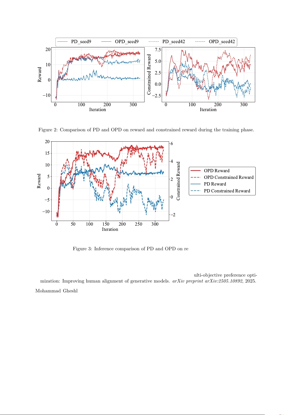
Pro v able Last-Iterate Con v ergence for Multi-Ob jectiv e Safe LLM Alignmen t via Optimistic Primal-Dual Yining Li 1 , P eizhong Ju 2 , and Ness Shroff 1 1 The Ohio State Univ ersity 2 Univ ersity of Ken tuc ky Abstract Reinforcemen t Learning from Human F eedbac k (RLHF) plays a significan t role in aligning Large Language Mo dels (LLMs) with h uman preferences. While RLHF with exp ected rew ard constraints can b e formulated as a primal–dual optimization problem, standard primal–dual metho ds only guar- an tee the conv ergence with a distributional p olicy where the saddle-point problem is in the con vex- conca ve form. Moreov er, standard primal-dual metho ds may exhibit instabilit y or divergence in the last iterations under p olicy parameterization in practical applications. In this w ork, we prop ose a univ ersal primal–dual framew ork for safe RLHF that unifies a broad class of existing alignment al- gorithms, including safe-RLHF, one-shot, and multi-shot based metho ds. Building on the univ ersal primal-dual framework, w e introduce an optimistic primal–dual (OPD) algorithm that incorp orates predictiv e up dates for b oth primal and dual v ariables to stabilize saddle-p oint dynamics. W e establish last-iterate con vergence guarantees for the prop osed method, cov ering both exact policy optimization in the distributional space and conv ergence to the neighborho o d of the optimal solution whose gap is related to approximate error and bias with parameterized p olicies. Our analysis reveals that opti- mism pla ys a crucial role in mitigating the oscillations inheren t to constrained alignmen t ob jectiv es, thereb y closing a key theoretical gap b etw een constrained RL and practical RLHF. 1 In tro duction The unsafe b ehaviors of large language mo dels (LLMs) ha ve raised growing concerns about the need to align safe and useful mo dels. Although LLMs hav e shown impressiv e p erformance across a wide range of language tasks, suc h as summarization Zhang et al. (2024), translation Elshin et al. (2024), and co de generation W ang and Chen (2023), they can also exhibit harmful b eha viors, including generating misleading or incorrect information Guerreiro et al. (2023); Zhang et al. (2025b), pro ducing inappropriate or toxic conten t W en et al. (2023), and leaking sensitive or priv ate data F eretzakis and V erykios (2024). As a result, aligning LLMs with human preferences that jointly emphasize helpfulness and safety has b ecome a critical challenge. In practice, preferences inv olv e m ultiple attributes, such as helpfulness, conciseness, factuality , and harmlessness, and these attributes are often not p erfectly aligned and can ev en conflict with one an- other Sorensen et al. (2024). How ev er, standard Reinforcemen t Learning from Human F eedback (RLHF) is inherently single-ob jective and does not fully capture the complexity of h uman preferences Ziegler et al. (2019); Stiennon et al. (2020). In its t ypical form, RLHF aligns a language mo del by collecting pairwise comparisons from human annotators, learning a rew ard mo del that reflects these preferences, and then optimizing the mo del to maximize the learned reward. This observ ation naturally motiv ates constrained RLHF, where the mo del is optimized for helpfulness while explicitly enforcing safety-related constraints. F or example, Dai et al. (2024); Huang et al. (2022); Du et al. (2025) study how to maximize the helpfulness reward while requiring the expected safet y cost to sta y b elow a predefined threshold. W e prop ose a universal framew ork that unifies a broad class of constrained RLHF algorithms based on Lagrangian relaxation Dai et al. (2024); Huang et al. (2024); Zhang et al. (2025a). These metho ds form ulate constrained RLHF as a saddle-p oint problem ov er a policy and a set of non-negative dual v ariables. Our framew ork unifies these approac hes by explicitly characterizing how different algorithms (i) approximately solve the primal p olicy optimization problem induced by the current dual v ariables, and (ii) up date the dual v ariables using feedbac k from constraint violations. 1 This unified p ersp ective highligh ts several algorithmic c haracteristics of existing approaches, including the con vergence b ehavior of primal–dual metho ds and the computational requiremen ts of one-shot and m ulti-shot pro cedures. In practice, naiv e primal–dual up dates Dai et al. (2024) can lead to unstable saddle-p oin t dynamics. Even in simple bilinear saddle-p oin t problems, simultaneous primal–dual updates fail to conv erge in the last iterate and guarantee only av erage conv ergence, meaning that optimalit y is ac hieved only when a veraging ov er iterates. This is often insufficien t in safe RLHF, where the deploy ed mo del corresp onds to the last iterate of training. Multi-shot metho ds can b e computationally exp ensive, as they require rep eatedly solving the primal p olicy optimization problem to near optimality for each dual up date Zhang et al. (2025a). Mean while, one-shot dualization-based approaches rely on choosing the closed-form solution in the space of distributional p olicies as the primal optimal p olicy Huang et al. (2024). While this assumption enables efficient dual optimization, it do es not accurately reflect practical alignmen t settings, where p olicies are parameterized b y large neural net works and the exact distributional optim um may be unattainable. These observ ations bring up an op en question: Is it p ossible to design an iter ative alignment algorithm for c onstr aine d RLHF that is b oth c omputational ly pr actic al and pr ovably stable in the last iter ate, without r elying on one-shot dualization or inner-lo op optimal p olicy solvers? T o address the stabilit y issue, w e propose an optimistic primal–dual metho d for safe RLHF. Optimistic primal–dual metho ds are known to stabilize saddle-p oin t dynamics and admit last-iterate conv ergence guaran tees Ding et al. (2023). Motiv ated b y this observ ation, w e propose an optimistic safe RLHF algorithm that augments both primal and dual up dates with optimistic steps. These steps predict future gradien ts, and the final up dates are obtained by correcting the predicted tra jectories, leading to more stable training and improv ed last-iterate p erformance. Our main con tributions include t wo parts. First, building on the prop osed unified primal–dual frame- w ork, we dev elop an optimistic primal–dual algorithm for safe RLHF. By incorp orating optimistic up- dates for both the p olicy and the dual v ariables, the prop osed metho d stabilizes saddle-point dynamics and mitigates the oscillatory b ehavior in the constrained alignmen t problems. Second, we establish theo- retical guarantees for the prop osed optimistic primal–dual algorithm. In the distributional p olicy space, w e show that the optimistic primal–dual metho d achiev es last-iterate conv ergence to an optimal solu- tion. W e further extend the analysis to parameterized p olicy spaces relev an t to practical LLM alignmen t, where w e prov e that the last iterate conv erges to a neighborho o d of the optimal solution. The resulting residual error is explicitly c haracterized in terms of statistical estimation error and parameterization bias. 2 Preliminaries on Constrained RLHF 2.1 Constrained RLHF Problem T o align with human preferences that inv olv e multiple, p otentially conflicting ob jectives, multi-ob jective or constrained v arian ts of RLHF hav e b een widely studied, where alignment is performed with resp ect to a primary ob jectiv e while additional preference dimensions are enforced via constrain ts. These v ariants largely follow the standard RLHF pip eline, which consists of sup ervised fine-tuning (SFT) to obtain a reference p olicy , learning reward mo dels from human preference data, and reinforcement-learning-based p olicy optimization with KL regularization to the reference mo del Ziegler et al. (2019); Stiennon et al. (2020). Let X and Y denote the sets of prompts and resp onses, resp ectiv ely . A language model is represented as a sto chastic policy mapping from the prompt set X to the distribution on the resp onse set Y , denoted as π : X → ∆( Y ), where ∆( Y ) is the set of all distributions on Y . Denote π ref as the reference p olicy obtained after SFT. W e consider multiple preference ob jectiv es indexed by K = S ∪ H , where ob jectives in S are optimized and those in H are enforced via constraints. T o learn a reward mo del for ob jective k , w e assume access to a h uman preference dataset { ( x i k , y i,w k , y i,l k ) } N i =1 , where x i k is a prompt and ( y i,w k , y i,l k ) denotes a preferred (indicated b y sup erscript w ) and less preferred (indicated by sup erscript l ) resp onse pair annotated by human annotators. F ollo wing standard practice in RLHF, we assume that preferences are generated according to a laten t reward function R ∗ k ( x, y ), and that human comparisons follow the Bradley-T erry mo del Ouyang et al. (2022): P ( y w ≻ y l | x ) = σ  R ∗ k ( x, y w ) − R ∗ k  x, y l  , where σ ( · ) denotes the sigmoid function. The reward model is then estimated by maximum likelihoo d 2 o ver the preference dataset, R k = arg max R N X i =1 log σ  R  x i k , y i,w k  − R  x i k , y i,l k  . F or the constrained ob jectives indexed by H , we specify a v ector of thresholds b = ( b j ) j ∈H , whic h define minimum p erformance requirements. F or notational conv enience, w e absorb the thresholds in to the reward definitions b y in tro ducing shifted rewards ˜ R j ( x, y ) := R j ( x, y ) − b j , and with a slight abuse of notation, we contin ue to denote the shifted rew ards by R j . The goal of RLHF is to optimize a p olicy with resp ect to the learned reward signals while regularizing it to remain close to a reference p olicy . Giv en a preference w eight vector w ∈ R |S | + suc h that P k ∈S w k = 1, enco ding the user’s trade-off ov er the soft ob jectives in S , the resulting m ulti-ob jective RLHF problem is formulated as max π E x ∼D " E y ∼ π ( ·| x ) " X k ∈S w k R k ( x, y ) # − β KL ( π ( ·| x ) ∥ π ref ( ·| x ))] s.t. E x ∼D ,y ∼ π ( ·| x ) [ R j ( x, y )] ≥ 0 , ∀ j ∈ H , where D denotes the prompt distribution and β > 0 controls the w eight of KL regularization to the reference p olicy π ref . 2.2 Lagrangian Metho d A standard approach to solving constrained RLHF problems is the Lagrangian metho d. F or eac h con- strained ob jective j ∈ H , we introduce a nonnegative Lagrange m ultiplier λ j ≥ 0. Given the preference w eights w ov er the soft ob jectives, w e define the aggregated reward S λ ( x, y ) := X k ∈S w k R k ( x, y ) + X j ∈H λ j R j ( x, y ) . (1) The resulting Lagrangian of the constrained m ulti-ob jective RLHF problem is L ( π , λ ) = E x ∼D , y ∼ π ( ·| x ) [ S λ ( x, y )] − β E x ∼D [KL( π ( ·| x ) ∥ π ref ( ·| x ))] . The corresp onding saddle-p oint problem is min λ ≥ 0 max π L ( π , λ ) . (2) When optimizing ov er the space of all sto chastic p olicies, the ob jective is concav e in π and linear in λ , and the problem admits a conv ex–concav e structure. In this case, for any fixed λ , the optimal p olicy has a closed-form solution given by π ⋆ ( y | x ) = π ref ( y | x ) exp ( S λ ( x, y ) /β ) / Z ( x ) , (3) where Z ( x ) is the normalization factor Z ( x ) = P y π ref ( y | x ) exp ( S λ ( x, y ) /β ). Detailed deriv ations are pro vided in theorem B.7. In practice, how ever, the policy is restricted to a parameterized family { π θ } θ ∈ Θ , under which the optimization b ecomes non-concav e in θ . As a result, practical constrained RLHF algo- rithms t ypically rely on iterativ e primal–dual updates, alternating betw een approximate p olicy optimiza- tion for fixed λ and gradien t-based up dates of the dual v ariables. The conv ergence of suc h metho ds in the parameterized setting generally requires additional assumptions or sp ecialized algorithmic designs. Fixing the p olicy π , the Lagrangian is differen tiable with resp ect to the dual v ariables. The gradient of L ( π , λ ) with respect to λ j is given by ∇ λ j L ( π , λ ) = E x ∼D , y ∼ π ( ·| x )  R j ( x, y )  . Accordingly , standard constrained RLHF methods update the dual v ariables b y pro jected gradient de- scen t, i.e., mo ving λ in the direction of constraint violation and pro jecting on to R ≥ 0 . 3 2.3 A univ ersal safe RLHF framework W e propose a univ ersal framew ork that unifies a broad class of constrained RLHF algorithms based on Lagrangian re- laxation. The detailed universal Lagrangian alignment framew ork is sho wn in 1. Algorithm 1 Univ ersal Lagrangian Alignment F ramework Require: Prompt distribution D ; Reward models { R k ( x, y ) } k ∈K ; soft weigh ts { w j } j ∈S ; reference p olicy π ref ; KL co efficient β ; initial θ 0 , λ 0 ≥ 0; 1: for t = 0 , 1 , 2 , . . . , T − 1 do 2: Primal up date: 3: π θ t +1 ← PrimalOracle ( π θ t , λ t , π ref , D , β ) 4: Dual up date: 5: g t ← GradEst ( θ t +1 , λ t , π ref , D ) 6: λ t +1 ← h λ t − 1 η λ g t i + 7: end for 8: Return λ T and θ T . F or eac h iteration, the framew ork alternates b et ween a primal up date and a dual up date. (1) The primal up date is abstracted as a PrimalOra cle , which aims to maximize the Lagrangian ob jectiv e for a giv en dual v ariable. Dep ending on the choice of the oracle, the primal step may corresp ond to a single-step or multi-step p olicy gradient up date in the parameter space, an appro ximate inner-iterations to solve the near-optimal p olicy in the parameterization space, or an exact closed-form solution in the distribution space Huang et al. (2024). (2) The dual up date use GradEst estimates the exp ected rew ards of the constrained ob jectives under the current p olicy , follow ed by a pro jected gradien t step on the dual v ariable. Differen t existing alignment metho ds can b e reco vered by instantiating the primal oracle and the dual gradient estimator differently , as detailed b elow. • Finite-step primal–dual updates. When the primal oracle p erforms a finite n umber of sto chastic gradien t steps, the algorithm reduces to the class of coupled primal–dual metho ds used in safe RLHF and constrained DPO Dai et al. (2024); Du et al. (2025); Liu et al. (2024). In this regime, the primal p olicy is up dated by a small n umber of sto chastic gradient steps under a non-stationary ob jective induced by the evolving dual v ariable. These metho ds lack last-iterate con vergence guarantees, ev en when the underlying Lagrangian is conv ex–concav e in the distribution space. • Approximate multi-shot v ariants. Some recent works decouple the optimization b y introducing an outer-lo op dual up date and an inner-lo op primal optimization that approximately maximizes the Lagrangian for a fixed dual v ariable Zhang et al. (2025a). While this reduces interference b et ween primal and dual up dates, the inner-lo op problem remains non-conv ex in the parameter space and is only solved appro ximately , which preven ts these metho ds from b eing interpreted as exact primal oracles. • Exact dualization and one-shot alignment. In contrast, one-shot metho ds are obtained by analyti- cally eliminating the primal v ariable in the distribution space, whic h yields an explicit, closed-form, and conv ex dual ob jective Huang et al. (2024). They can b e view ed as a degenerate instantiation of the universal framework: the primal oracle returns the closed-form optimal distributional p olicy for a given dual v ariable, so no iterative primal updates are required during dual optimization. Therefore, each iteration reduces to a pure dual up date step. 3 Optimistic Primal–Dual Metho d Standard primal–dual metho ds do not guarantee last-iterate conv ergence in constrained RLHF, and this fundamen tal limitation motiv ates the need for alternativ e primal–dual metho ds with stronger stability prop erties. The univ ersal framework in algorithm 1 formulates constrained RLHF as a Lagrangian saddle-p oin t problem, where the primal up date optimizes the p olicy and the dual up date adjusts the constrain t multipliers. When optimization is carried out ov er the distributional p olicy space, the KL regularization induces strong conca vity in the primal v ariable. How ev er, the Lagrangian remains linear 4 Algorithm 2 OPD with Primal Distributional Policies Require: Prompt distribution D ; Reward models { R k ( x, y ) } k ∈K ; soft weigh ts { w j } j ∈S ; reference p olicy π ref ; KL co efficient β ; initial ˆ π 0 , λ 0 ≥ 0; 1: for t = 0 , 1 , 2 , . . . , T − 1 do 2: Primal Optimistic Up date: π t = arg max π ( L ( π , λ t − 1 ) − E x ∼D [ η θ KL ( π ( ·| x ) ∥ ˆ π t ( ·| x ))]) , (4) 3: Dual Optimistic Up date: λ t = arg min λ ≥ 0 λ E x ∼D ,y ∼ π t − 1 ( ·| x ) [ R ( x, y )] + η λ ( λ − ˆ λ t ) 2 , (5) 4: Primal Actual Up date: ˆ π t +1 = arg max π L ( π , λ t ) − E x ∼D [ η θ KL ( π ( ·| x ) ∥ ˆ π t ( ·| x ))] , (6) 5: Dual Actual Up date: ˆ λ t +1 = arg min λ ≥ 0 λ E x ∼D ,y ∼ π t ( ·| x ) [ R ( x, y )] + η λ ( λ − ˆ λ t ) 2 . (7) 6: end for 7: Return ˆ λ T and ˆ π T . in the dual multipliers, and hence the resulting saddle-p oint problem is generally not strongly-conv ex- strongly-conca ve. The gradient descen t-ascent methods conv erge linearly to the unique saddle p oint only under smooth strongly-conv ex-strongly-concav e conditions with appropriate step sizes Zamani et al. (2024). Once these conditions are violated, such guarantees no longer hold, and last-iterate conv ergence ma y fail ev en when a unique saddle p oint exists. Example: F ailure of Last-Iterate Conv ergence in a Bilinear Saddle-P oin t Problem W e consider a simple con vex–conca ve bilinear problem min y max x x T Ay , where A is a full-rank matrix whose singular v alues are [ σ 1 , · · · , σ M ]. The standard primal–dual gradient metho d gives x t +1 = x t + α Ay t and y t +1 = y t − α A ⊤ x t , where α is the stepsize. Let z t = [ x t , y i ] ⊤ . Then the up date can b e written as a linear iteration z t +1 = ( I − α J ) z t , J =  0 − A A ⊤ 0  . The matrix J has imaginary eigen v alues ± iσ i . Hence, ( I − α J ) has eigen v alues 1 ± iασ i whose magnitudes are larger than 1, implying that the last iterates do not contract tow ard the saddle p oint due to the saddle-p oin t problem’s inheren tly rotational structure Dask alakis and P anageas (2018). The aforemen tioned example implies that, ev en in constrained RLHF problems where the primal ob jective is strongly concav e ov er the distributional p olicy space, standard primal–dual metho ds gen- erally admit only av erage conv ergence guarantees and ma y fail to con verge in the last iterate. The situation b ecomes even more challenging in practical RLHF settings with parameterized policies, where the optimization problem is no longer con vex in the p olicy parameters. Motiv ated by these challenges, we adopt an optimistic primal–dual (OPD) metho d, which corrects eac h update using a prediction of the next-step gradient and is kno wn to suppress the rotational dynamics whic h can cause oscillations. In the follo wing, we first analyze OPD in the distributional p olicy space and establish last-iterate conv ergence to the optimal primal–dual solution. W e then extend the analysis to parameterized p olicies, showing that the same guarantees hold up to approximation errors. 3.1 OPD in Distribution Space OPD up date in distribution space is shown in eqs. (4) to (7) of algorithm 2. OPD introduces predictive 5 iterates ( π t , λ t ) to approximate the next-step primal and dual v ariables. The actual up dates ( ˆ π t +1 , ˆ λ t +1 ) are then corrected based on these predictions. W e make the following assumptions. theorem 3.1 corresp onds to Slater’s condition, which assumes the existence of a strictly feasible p olicy and guarantees strong duality , i.e., the existence of the optimal saddle p oint. Slater’s condition is standard in the analysis of constrained optimization and primal–dual metho ds Huang et al. (2024); Zhang et al. (2025a); Du et al. (2025). theorem 3.2 assumes that all reward mo dels are uniformly b ounded, which is a common condition in the RLHF literature Du et al. (2025). theorem 3.3 requires the reference p olicy to assign nonzero probability to every feasible action. F or LLM p olicies parameterized b y softmax distributions, token probabilities are strictly p ositiv e ov er the mo deled action set. When action masking or filtering is applied, we equiv alen tly redefine the action space as the accessible set and require the reference p olicy to hav e full supp ort on this restricted space. Assumption 3.1 (Slater’s condition) . There exists a p olicy ¯ π ∈ Π and a constan t ξ > 0 such that E x ∼D ,y ∼ ¯ π [ R j ( x, y )] ≥ ξ , ∀ j ∈ H . Assumption 3.2 (Bounded rewards) . There exists R max > 0 such that   R k ( x, y )   ≤ R max for all k ∈ K , x ∈ X , and y ∈ Y . Assumption 3.3 (F ull support of the reference p olicy) . Assume the reference p olicy has the full supp ort, i.e., there exists p min > 0 such that π ref ( y | x ) ≥ p min for any ( x, y ) pair. theorem 3.3 ensures that p olicy supp orts do not collapse along the OPD iterates and that all KL div ergence terms remain well-defined throughout optimization. W e initialize ˆ π 0 = π ref , and all subsequent p olicy up dates are obtained via KL-regularized maximization. Hence, the supp ort of ˆ π t ( ·| x ) remains con tained within that of the reference p olicy for all t . Moreo ver, any optimal p olicy π ⋆ satisfying the constrain ts is co v ered b y the reference support and b y the supp orts of the OPD iterates. This assumption prev ents premature elimination of feasible actions and guarantees that OPD op erates ov er a p olicy class that contains the optimal solution. Theorem 3.4. Under the or em 3.1, the or em 3.2, and the or em 3.3, under suitably chosen hyp er-p ar ameters η θ and η λ (e.g., η θ = η λ = 3 p |H| R max ), then the optimistic primal–dual iter ates of e qs. (4) to (7) satisfy E x ∼D [KL( π θ ⋆ ( ·| x ) ∥ ˆ π t ( ·| x ))] + ∥ λ ⋆ − ˆ λ t ∥ 2 2 ≤ ρ t − 1 Φ 1 min  η θ + β , 7 4 η λ − 3 4 p |H| R max  , wher e 0 < ρ < 1 is define d in e q. (46) and Φ 1 is a c ostant define d as e q. (47) . theorem 3.4 establishes a linear last-iterate conv ergence guarantee for OPD in the p olicy distribution space. The final iterates ( ˆ π t , ˆ λ t ) conv erge linearly tow ard the optimal saddle point ( π ⋆ , λ ⋆ ) at rate ρ < 1, as measured b y the KL div ergence in the primal v ariable and the squared ℓ 2 error in the dual v ariable. In contrast to standard primal–dual metho ds that typically only ensure ergo dic conv ergence, this result provides direct control ov er the final p olicy iterate, whic h is particularly imp ortant in safe RLHF, where constrain t satisfaction and alignment quality are ev aluated on the deplo yed p olicy rather than on an av erage of iterates. Moreo ver, the result holds under a linear dual ob jective and without strong conv exit y in the dual v ariable, highligh ting the stabilizing effect of the optimistic primal–dual up dates. 3.2 OPD in P arameter Space 3.2.1 OPD Up dates in the Parameterized P olicy Space In the parameterized p olicy space, where the p olicy is represented as π θ with parameters θ ∈ Θ, the resulting Lagrangian optimization problem is generally non-conv ex and the closed-form distributional up dates in eqs. (4) and (6) are no longer tractable. W e therefore adopt a gradient-based optimistic primal–dual metho d in the parameter space. W e denote the parameterized counterparts of π t and ˆ π t b y π θ t and π ˆ θ t , resp ectively . T o obtain a tractable update consisten t with the distributional form ulation sho wn in eqs. (4) and (6), we approximate the KL divergence b y its second-order T aylor expansion around ˆ θ t . Sp ecifically , when θ t is sufficiently 6 Algorithm 3 OPD with Primal Parameterized Policies Require: Prompt distribution D ; Reward models { R k ( x, y ) } k ∈K ; soft weigh ts { w j } j ∈S ; reference p olicy π ref ; KL co efficient β ; initial ˆ θ 0 , λ 0 ≥ 0; 1: for t = 0 , 1 , 2 , . . . , T − 1 do 2: Primal Optimistic Up date: θ t = Pro j Θ  ˆ θ t + 1 η θ + β F ( ˆ θ t ) † ∇ θ L ( π ˆ θ t , λ t − 1 )  . (8) 3: Dual Optimistic Up date: λ t =  ˆ λ t − 1 η λ E x ∼D , y ∼ π θ t − 1 ( ·| x ) [ R ( x, y )]  + . (9) 4: Primal Actual Up date: ˆ θ t +1 = Pro j Θ  ˆ θ t + 1 η θ + β F ( ˆ θ t ) † ∇ θ L ( π ˆ θ t , λ t )  . (10) 5: Dual Actual Up date: ˆ λ t +1 =  ˆ λ t − 1 η λ E x ∼D , y ∼ π θ t ( ·| x ) [ R ( x, y )]  + . (11) 6: end for 7: Return ˆ λ T and π ˆ θ T . close to ˆ θ t , we hav e E x ∼D h KL  π θ t ( ·| x ) ∥ π ˆ θ t ( ·| x ) i ≈ 1 2 ( θ t − ˆ θ t ) ⊤ F ( ˆ θ t )( θ t − ˆ θ t ) , where F ( θ ) denotes the Fisher information matrix, F ( θ ) = E x ∼D ,y ∼ π θ ( ·| x )  ∇ θ log π θ ( y | x ) ∇ θ log π θ ( y | x ) ⊤  . T o accommo date p ossible rank deficiency , w e use the Mo ore-P enrose pseudo-inv erse F ( θ ) † . Under this lo cal appro ximation, the distributional OPD updates reduce to natural policy gradient (NPG) steps in the parameter space. T o ensure feasibility in the parameter domain, we pro ject the up dated parameters bac k onto the parameter space Θ after eac h primal up date. Similar to algorithm 2, the prop osed metho d first p erforms optimistic primal and dual up dates to predict the next-step p olicy parameters and dual v ariables, as shown in eqs. (8) and (9). The actual primal and dual updates are then carried out using these predictions, as specified in eqs. (10) and (11). The complete OPD pro cedure in the parameterized p olicy space is summarized in algorithm 3. The parameterized OPD applies optimism asymmetrically across the primal and dual v ariables. In particular, the predicted p olicy iterate π θ t is only used to form the dual up dates λ t and ˆ λ t +1 , whereas the actual policy π ˆ θ t is used for the primal up dates θ t and ˆ θ t +1 . This asymmetric design ensures that p olicy-gradien t computations are performed only for the actual p olicy updates, while the predicted policy iterate π θ t is used solely for ev aluation in the dual up dates and do es not require gradient computation. In con trast, symmetric extragradient metho ds Ding et al. (2023) typically require ev aluating b oth primal and dual op erators at the predictor iterate, resulting in higher computational cost and v ariance. R emark 3.5 (Equiv alence b etw een Distribution-Space OPD and NPG Up dates) . Under tabular softmax parameterization, the distribution-space OPD up dates in eqs. (4) to (7) are equiv alent to their parameter- space coun terparts in eqs. (8) to (11). In particular, for all t , the induced p olicies satisfy π θ t = π t and π ˆ θ t +1 = ˆ π t +1 . The k ey observ ation is that, under tabular softmax parameterization, p olicy parameters θ are in one-to-one corresp ondence with p olicy distributions. Moreov er, KL-regularized optimization in the dis- tribution space is exactly equiv alen t to mirror descent under the KL geometry , which corresp onds to NPG up dates in the parameter space. As a result, the distribution-space OPD up dates generate exactly the same sequence of p olicies as the NPG-based OPD updates. 7 0.0 0.2 0.4 0.6 0.8 1.0 ( 0 ) 0.0 0.5 1.0 1.5 2.0 2.5 PD OPD Optimal 0 200 400 600 800 1000 iteration 1 0 6 1 0 4 1 0 2 1 0 0 d i s t a n c e t o ( ( 0 ) * , * ) PD OPD Figure 1: Comparison of OPD and PD under a softmax tabular parameterization in a single-state, tw o- action RLHF toy problem. OPD (red) conv erges to the optimal solution in the last iterate, while PD (blue) exhibits p ersistent oscillations and fails to conv erge. R emark 3.6 (Relationship to PPO in Practice) . NPG controls p olicy up dates b y explicitly constrain- ing the KL div ergence b etw een consecutive p olicies, while proximal p olicy optimization (PPO) enforces up date stabilit y by directly clipping the p olicy ratio. Although the tw o approaches differ in their for- m ulations, b oth can b e interpreted as mechanisms for b ounding p olicy up dates and preven ting o verly aggressiv e p olicy changes. In practice, PPO is often preferred due to its simplicity and empirical robust- ness, and the prop osed OPD framework can b e implemented using PPO-st yle clipp ed up dates. In this pap er, we adopt the NPG form ulation for analytical conv enience, as it provides a clean connection to KL-regularized optimization and facilitates theoretical analysis. In our experiments, w e implement the prop osed OPD framework using PPO-st yle up dates. 3.2.2 A T oy RLHF Example Illustrating the Stabilit y of OPD W e consider a minimal RLHF-st yle constrained optimization problem with a single state ( |X | = 1) and t wo actions ( |Y | = 2), denoted b y y 0 and y 1 . Since there is only one state, w e omit the dep endence on x in the following. W e consider tw o reward mo dels. The first reward R s represen ts the ob jectiv e to b e maximized, while the second rew ard R h corresp onds to a safety-related constraint. W e set R s ( y 0 ) = 1 and R s ( y 1 ) = 0, so that the expected rew ard under a policy π is simply π ( y 0 ). F or the constrain t rew ard, w e c ho ose R h ( y 0 ) = − 0 . 7 and R h ( y 1 ) = 0 . 3, whic h induces the constrain t − 0 . 7 π ( y 0 ) + 0 . 3 (1 − π ( y 0 )) ≥ 0, or equiv alen tly π ( y 0 ) ≤ 0 . 3. W e select the reference policy as π ref ( y 0 ) = 0 . 3. The resulting optimization problem is to maximize π ( y 0 ) − β KL( π ( · ) ∥ π ref ( · )) sub ject to π ( y 0 ) ≤ 0 . 3 , with β = 0 . 05. It is easy to verify that the optimal p olicy coincides with the reference p olicy π ref . T o av oid explicit pro jection on to the p olicy simplex, w e adopt a softmax parameterization π ( y 0 ) = 1 / (1 + exp( θ )). W e set the effectiv e primal stepsize α = ( η θ + β ) − 1 = 0 . 6 and the dual stepsize η − 1 λ = 0 . 6. Figure 1 compares the tra jectories of OPD and standard primal–dual updates under this parameteriza- tion. As shown in fig. 1, the proposed OPD metho d con v erges to the optimal saddle p oin t, with the distance to the optimum decreasing linearly , consisten t with the theoretical guarantees in theorem 3.4. In contrast, the standard PD up dates fail to con verge and exhibit divergen t b ehavior in this simple setting. 3.2.3 Theoretical Results Let Π Θ denote the class of parameterized p olicies that ha ve full supp ort on the considered action set, i.e., there exists p min > 0 such that π θ ( y | x ) ≥ p min for all feasible ( x, y ). W e further assume that the 8 parameter domain Θ ⊂ R d is closed and conv ex, so that the pro jection op erator Pro j Θ ( · ) used in the up dates is well-defined. Since our analysis fo cuses on optimalit y within the parameterized p olicy class, w e imp ose a Slater-t ype condition in the parameterized p olicy space. Assumption 3.7 (Slater’s condition in the parameterized policy space) . There exists a parameter v ector ¯ θ ∈ Θ and a constan t ξ > 0 such that the corresp onding policy π ¯ θ ∈ Π Θ satisfies E x ∼D ,y ∼ π ¯ θ ( ·| x ) [ R j ( x, y )] ≥ ξ , ∀ j ∈ H . theorem 3.8 assumes that the log-p olicy is Lipsc hitz con tinuous with respect to the policy parameters. This condition allows us to translate deviations in the parameter space into controlled changes in the induced policy distributions, and is particularly useful for b ounding KL divergence and log-ratio terms that arise in the analysis. Such an assumption is standard in the analysis of p olicy gradient and mirror descen t metho ds with parameterized p olicies. Assumption 3.8 (Log-policy Lipschitz contin uity) . There exists a constant C > 0 such that for any θ 1 , θ 2 ∈ Θ, E x ∼D , y ∼Y ( x ) [ | log π θ 1 ( y | x ) − log π θ 2 ( y | x ) | ] ≤ C ∥ θ 1 − θ 2 ∥ 1 . As the primal up dates rely on sto chastic gradien t estimates and empirical Fisher information com- puted from finite samples, we make the follo wing assumption to quantify the inexactness arises naturally in practice. Assumption 3.9 (Inexact primal up dates) . Let θ ∗ t and ˆ θ ∗ t +1 denote the exact primal up dates defined b y eqs. (8) and (10) when all exp ectations are computed exactly . Due to sto chastic estimation and n umerical approximation, the implemented up dates pro duce θ t and ˆ θ t +1 suc h that, for all t , E [ ∥ θ t − θ ∗ t ∥ 1 ] ≤ ϵ approx , E h ∥ ˆ θ t +1 − ˆ θ ∗ t +1 ∥ 1 i ≤ ϵ approx . Suc h p er-iteration errors are standard in the analysis of sto c hastic mirror descent and natural p olicy gradien t metho ds. In the tabular setting with exact expectations, this approximation error v anishes, i.e., ϵ approx = 0. F or parameterized p olicies, ϵ approx captures the combined effects of sampling noise and n umerical approximation, and can b e made arbitrarily small with sufficiently large batch sizes. Corollary 3.10. Under the or em 3.2, the or em 3.3, the or em 3.7, the or em 3.8 and the or em 3.9, under suitably chosen hyp er-p ar ameters η θ and η λ (e.g., η θ = η λ = 3 p |H| R max ), then the optimistic primal– dual iter ates of e qs. (8) to (11) satisfies E x ∼D [KL( π θ ⋆ ( ·| x ) ∥ ˆ π t ( ·| x ))] + ∥ λ ⋆ − ˆ λ t ∥ 2 2 ≤ ρ t − 1 Φ 1 min  η θ + β , 7 4 η λ − 3 4 p |H| R max  + 2(1 − ρ t ) 1 − ρ gap( ε approx , p min ) , wher e 0 < ρ < 1 is define d in e q. (46) and Φ 1 is define d as e q. (47) , and gap( ε approx , p min ) is define d in e q. (28) . The additional error term gap( ε approx , p min ) c haracterizes the error gap induced by function approx- imation and finite-sample estimation in the p olicy up date, and it determines the radius of a b ounded neigh b orho o d around the optimal saddle point ( π ⋆ , λ ⋆ ). The geometric con traction factor ρ t − 1 with 0 < ρ < 1 ensures last-iterate conv ergence. OPD in the parameter space preserv es geometric last-iterate con vergence, implying that function appro ximation do es not destroy the stabilizing effect of optimism, but only in tro duces a controlled residual error. As the approximation error v anishes, the neighborho o d shrinks accordingly . This result establishes OPD as a robust framework for constrained RLHF under practical p olicy parameterizations. 9 4 Computational Exp erimen ts In this section, we empirically ev aluate the effectiveness and robustness of the prop osed OPD-based metho ds for aligning helpfulness and harmlessness. Specifically , our exp eriments are designed to answer the following questions: • How robust is the training pro cess of the prop osed OPD-based method compared to standard PD-based approaches? • Do es improv ed training stability translate into sup erior p erformance at ev aluation time? Datasets and Rew ard Models W e adopt the Alpaca-7b-repro duced mo del as the reference p olicy throughout our exp eriments. F or mo del-based alignment, we directly use the beaver-7b-v1.0-reward and beaver-7b-v1.0-cost models released with Safe-RLHF Dai et al. (2024) as the rew ard mo del for the target ob jective and the safety mo del for the constraint, resp ectively . Note that the original Safe-RLHF form ulation enforces the cost to b e smaller than zero; to match our constraint conv en tion, we negate the cost mo del outputs. W e conduct our exp eriments on the PKU-SafeRLHF-30K preference dataset Dai et al. (2024), which contains appro ximately 27K training prompts and 3K test prompts, eac h paired with a preferred and a less-preferred resp onse. In addition to preference lab els, the dataset provides safety annotations, where preferences are determined join tly based on helpfulness and harmlessness. OPD implementation On the primal side, w e follow the standard PPO-style implemen tation used in practical RLHF systems. Sp ecifically , the p olicy up date is implemented via a clipp ed policy gradien t ob jective, which can b e view ed as a practical appro ximation of NPG under a trust-region constrain t induced by the KL div ergence to the reference p olicy . This design ensures stable p olicy updates while remaining compatible with large-scale language model fine-tuning. On the dual side, the dual v ariable λ is up dated using gradient ascent in the logarithmic parameter- ization log λ to enforce non-negativity and improv e n umerical stability . W e store the dual gradient from the previous iteration and construct an e xtrap olated gradien t using an extragradient-st yle correction. The effective up date direction is giv en by g OPD t = 2 g t − g t − 1 , where g t denotes the gradient of the dual ob jectiv e at iteration t . This corrected gradien t is applied directly to the log-dual v ariable log λ , yielding an optimistic update that anticipates future primal re- sp onses. Our OPD implemen tation explicitly introduces temporal coupling across iterations through gradien t reuse. W e set b oth the actor and critic learning rates to 5 × 10 − 5 , and the stepsize for the dual v ariable λ to 0 . 5. These relatively aggressive stepsizes inten tionally place PD-based metho ds in an unstable regime, allo wing us to test the robustness of the proposed OPD up dates. As sho wn in fig. 2, the OPD metho d con verges to p olicies that satisfy the safety constraints while maintaining comp etitive rewards, whereas PD-based metho ds exhibit degraded safet y p erformance at con vergence. W e conduct mo del-based ev aluations for both helpfulness and safety , as sho wn in fig. 3. Specif- ically , the generated resp onses are ev aluated by computing the corresp onding av erage helpfulness and safet y scores using the pro xy rew ard and safet y mo dels. The ev aluation results sho w that the OPD-based metho d ac hiev es higher rew ards and constraints than PD-based methods, indicating that improv ed train- ing stability translates into sup erior ev aluation p erformance. 5 Conclusion W e dev elop a univ ersal primal–dual framework that unifies a broad class of Lagrangian approaches to constrained RLHF. Building on this framew ork, we prop ose an OPD algorithm that introduces predictiv e up dates for b oth the primal p olicy and the dual multipliers to stabilize saddle-p oint dynamics. W e establish last-iterate con vergence in b oth the distributional p olicy space and the parameterized p olicy space. In the distributional setting, the iterates conv erge to the exact saddle p oint; in the parameterized setting, they conv erge to a neighborho o d of the optimum. W e compare standard primal–dual training with our OPD v arian t. With more aggressiv e step sizes, OPD exhibits impro v ed training stabilit y relativ e to PD, and this stability translates into b etter p erformance in ev aluations. 10 0 100 200 300 Iteration 10 0 10 20 Reward 0 100 200 300 Iteration 2.5 0.0 2.5 5.0 7.5 Constrained Reward PD_seed9 OPD_seed9 PD_seed42 OPD_seed42 Figure 2: Comparison of PD and OPD on rew ard and constrained rew ard during the training phase. 0 50 100 150 200 250 300 Iteration 10 5 0 5 10 15 20 Reward OPD Reward OPD Constrained Reward PD Reward PD Constrained Reward 2 0 2 4 6 Constrained Reward Figure 3: Inference comparison of PD and OPD on rew ard and cost. References Akhil Agnihotri, Rahul Jain, Deepak Ramac handran, and Zheng W en. Multi-ob jective preference opti- mization: Impro ving human alignment of generativ e mo dels. arXiv pr eprint arXiv:2505.10892 , 2025. Mohammad Gheshlaghi Azar, Zhaohan Daniel Guo, Bilal Piot, Remi Munos, Mark Rowland, Michal V alko, and Daniele Calandriello. A general theoretical paradigm to understand learning from human preferences. In International Confer enc e on A rtificial Intel ligenc e and Statistics , pages 4447–4455. PMLR, 2024. Josef Dai, Xuehai Pan, Ruiyang Sun, Jiaming Ji, Xinbo Xu, Mick el Liu, Yizhou W ang, and Y ao dong Y ang. Safe rlhf: Safe reinforcement learning from h uman feedback. In The Twelfth International Confer enc e on L e arning R epr esentations , 2024. Constan tinos Dask alakis and Ioannis P anageas. The limit p oints of (optimistic) gradient descen t in min-max optimization. A dvanc es in neur al information pr o c essing systems , 31, 2018. Guneet S Dhillon, Xing jian Shi, Y ee Why e T eh, and Alex Smola. L3ms–lagrange large language mo dels. arXiv pr eprint arXiv:2410.21533 , 2024. Dongsheng Ding, Chen-Y u W ei, Kaiqing Zhang, and Alejandro Rib eiro. Last-iterate con vergen t p ol- 11 icy gradient primal-dual metho ds for constrained mdps. A dvanc es in Neur al Information Pr o c essing Systems , 36:66138–66200, 2023. Dongsheng Ding, Kaiqing Zhang, Jiali Duan, T amer Basar, and Mihailo R Jov ano vic. Conv ergence and sample complexity of natural p olicy gradient primal-dual metho ds for constrained mdps. Journal of Machine L e arning R ese ar ch , 26(256):1–76, 2025. Yihan Du, Seo T aek Kong, and R Srik an t. Primal-dual direct preference optimization for constrained llm alignment. arXiv pr eprint arXiv:2510.05703 , 2025. Denis Elshin, Nikola y Karpachev, Boris Gruzdev, Ily a Golov ano v, Georgy Iv anov, Alexander An tonov, Nic kola y Sk achk o v, Ek aterina Latypov a, Vladimir Layner, Ek aterina Enikeev a, et al. F rom general llm to translation: How we dramatically improv e translation qualit y using human ev aluation data for llm finetuning. In Pr o c e e dings of the Ninth Confer enc e on Machine T r anslation , pages 247–252, 2024. Ka win Ethay ara jh, Winnie Xu, Niklas Muennighoff, Dan Jurafsky , and Dou we Kiela. Kto: Mo del alignmen t as prospect theoretic optimization. arXiv pr eprint arXiv:2402.01306 , 2024. Georgios F eretzakis and V assilios S V erykios. T rustw orth y ai: Securing sensitive data in large language mo dels. AI , 5(4):2773–2800, 2024. Nuno M Guerreiro, Duarte M Alv es, Jonas W aldendorf, Barry Haddow, Alexandra Birc h, Pierre Colom b o, and Andr ´ e FT Martins. Hallucinations in large multilingual translation mo dels. T r ans- actions of the Asso ciation for Computational Linguistics , 11:1500–1517, 2023. Jiw o o Hong, Noah Lee, and James Thorne. Orp o: Monolithic preference optimization without reference mo del. arXiv pr eprint arXiv:2403.07691 , 2024. Sandy Huang, Abbas Ab dolmaleki, Giulia V ez zani, Philemon Brakel, Daniel J Manko witz, Michael Neunert, Stev en Bohez, Y uv al T assa, Nicolas Heess, Martin Riedmiller, et al. A constrained multi- ob jective reinforcemen t learning framework. In Confer enc e on R ob ot L e arning , pages 883–893. PMLR, 2022. Xinmeng Huang, Sh uo Li, Edgar Dobriban, Osb ert Bastani, Hamed Hassani, and Dongsheng Ding. One-shot safet y alignment for large language mo dels via optimal dualization. A dvanc es in Neur al Information Pr o c essing Systems , 37:84350–84383, 2024. Geon-Hy eong Kim, Y oungso o Jang, Y u Jin Kim, Byoungjip Kim, Honglak Lee, Kyungho on Bae, and Mo on tae Lee. Safedp o: A simple approach to direct preference optimization with enhanced safet y . arXiv pr eprint arXiv:2505.20065 , 2025. Zixuan Liu, Xiaolin Sun, and Zizhan Zheng. Enhancing llm safet y via constrained direct preference optimization. arXiv pr eprint arXiv:2403.02475 , 2024. Long Ouyang, Jeffrey W u, Xu Jiang, Diogo Almeida, Carroll W ainwrigh t, P amela Mishkin, Chong Zhang, Sandhini Agarw al, Katarina Slama, Alex Ra y , et al. T raining language mo dels to follow instructions with human feedback. A dvanc es in neur al information pr o c essing systems , 35:27730–27744, 2022. Rafael Rafailo v, Arc hit Sharma, Eric Mitc hell, Christopher D Manning, Stefano Ermon, and Chelsea Finn. Direct preference optimization: Y our language mo del is secretly a reward mo del. A dvanc es in neur al information pr o c essing systems , 36:53728–53741, 2023. T aylor Sorensen, Jared Moore, Jillian Fisher, Mitchell Gordon, Nilo ofar Mireshghallah, Christo- pher Michael Rytting, Andre Y e, Liwei Jiang, Ximing Lu, Nouha Dziri, et al. A roadmap to pluralistic alignmen t. arXiv pr eprint arXiv:2402.05070 , 2024. Nisan Stiennon, Long Ouyang, Jeffrey W u, Daniel Ziegler, Ryan Low e, Chelsea V oss, Alec Radford, Dario Amo dei, and Paul F Christiano. Learning to summarize with human feedback. A dvanc es in neur al information pr o c essing systems , 33:3008–3021, 2020. Akifumi W achi, Thien T ran, Rei Sato, T akumi T anab e, and Y ouhei Akimoto. Step wise alignment for constrained language mo del p olicy optimization. A dvanc es in Neur al Information Pr o c essing Systems , 37:104471–104520, 2024. 12 Jianxun W ang and Yixiang Chen. A review on co de generation with llms: Application and ev aluation. In 2023 IEEE International Confer enc e on Me dic al A rtificial Intel ligenc e (Me dAI) , pages 284–289. IEEE, 2023. Jiaxin W en, Pei Ke, Hao Sun, Zhexin Zhang, Chengfei Li, Jinfeng Bai, and Minlie Huang. Un veiling the implicit toxicit y in large language mo dels. arXiv pr eprint arXiv:2311.17391 , 2023. Rui Y ang, Xiaoman Pan, F eng Luo, Shuang Qiu, Han Zhong, Dong Y u, and Jianshu Chen. Rewards- in-con text: multi-ob jective alignment of foundation mo dels with dynamic preference adjustment. In Pr o c e e dings of the 41st International Confer enc e on Machine L e arning , pages 56276–56297, 2024. Moslem Zamani, Hadi Abbaszadehp eiv asti, and Etienne de Klerk. Con vergence rate analysis of the gradien t descen t–ascent metho d for conv ex–conca ve saddle-p oint problems. Optimization Metho ds and Softwar e , 39(5):967–989, 2024. Botong Zhang, Sh uo Li, Ignacio Hounie, Osb ert Bastani, Dongsheng Ding, and Alejandro Ribeiro. Align- men t of large language mo dels with constrained learning. arXiv pr eprint arXiv:2505.19387 , 2025a. Y ang Zhang, Hanlei Jin, Dan Meng, Jun W ang, and Jingh ua T an. A comprehensive surv ey on pro cess-orien ted automatic text summarization with exploration of llm-based metho ds. arXiv pr eprint arXiv:2403.02901 , 2024. Y ue Zhang, Y afu Li, Leyang Cui, Deng Cai, Lemao Liu, Tingc hen F u, Xinting Huang, En b o Zhao, Y u Zhang, Y ulong Chen, et al. Siren’s song in the ai o cean: A surv ey on hallucination in large language mo dels. Computational Linguistics , pages 1–46, 2025b. Zhanh ui Zhou, Jie Liu, Jing Shao, Xiangyu Y ue, Chao Y ang, W anli Ouyang, and Y u Qiao. Beyond one-preference-fits-all alignment: Multi-ob jectiv e direct preference optimization. In Findings of the Asso ciation for Computational Linguistics: ACL 2024 , pages 10586–10613, 2024. Daniel M Ziegler, Nisan Stiennon, Jeffrey W u, T om B Brown, Alec Radford, Dario Amo dei, Paul Chris- tiano, and Geoffrey Irving. Fine-tuning language models from h uman preferences. arXiv pr eprint arXiv:1909.08593 , 2019. 13 A Related W orks This section summarizes the related w ork in the LLMs safet y alignment. Constrained Alignment for LLMs There is a growing b o dy of work that formulates safe RLHF as a constrained optimization problem, where helpfulness is maximized sub ject to safet y-related con- strain ts Dai et al. (2024); Huang et al. (2024); Zhang et al. (2025a). A representativ e approach is mo del- ing the safet y violations via an exp ected cost constraint and solving the resulting constrained ob jective using iterative primal-dual up dates Dai et al. (2024). Ho wev er, the primal-dual metho ds can b e compu- tationally expensive and ma y suffer from training instability and h yp erparameter sensitivit y Huang et al. (2024). T o mitigate these issues, Huang et al. (2024) lev erages the closed-form structure of the optimal distribution induced b y fixed dual v ariables, and optimizes a smooth dual ob jective to eliminate rep eated primal-dual policy iterations. This dualization-based metho d leads to more stable training in practice. In con trast, Zhang et al. (2025a) studies constrained alignment in the parameterized LLM p olicy space and dev elops an iterativ e dual-based alignmen t method that alternates b etw een maximizing the Lagrangian o ver the LLM p olicy parameters and p erforming dual descen t up dates. Dhillon et al. (2024) prop oses an interior p oint metho d and uses a relaxed log-barrier function to enforce constraints, thereby av oiding the oscillation b et ween primal and dual v ariables. Existing approaches stabilize training via simplifying the dual problem with the closed-form structure of the optimal p olicy distribution, solving near-optimal primal subproblems for eac h dual v ariable, or enforcing the constraints with the interior-point meth- o ds. How ev er, it is still an op en question of how to design iterative primal-dual up dates with pro v able last-iterate guarantees for constrained LLM alignmen t. RL-free Based Safety Alignmen t In parallel, a line of RL-free metho ds has b een proposed for preference alignmen t, whic h bypasses explicit reward mo del learning and p olicy optimization via rein- forcemen t learning, and instead directly optimize the p olicy using preference data Rafailov et al. (2023); Azar et al. (2024); Ethay ara jh et al. (2024); Hong et al. (2024); Y ang et al. (2024). Building up on these approac hes, several recent works prop ose constrained preference alignment in an RL-free manner Liu et al. (2024); W ac hi et al. (2024); Du et al. (2025); Kim et al. (2025). Among them, some metho ds still adopt a primal-dual persp ective and iteratively up date both the p olicy and the dual v ariables, while using Direct Policy Optimization (DPO)-style ob jectives as the primal optimizer Liu et al. (2024); Du et al. (2025). T o implicitly control the trade-off betw een reward and safet y using only rew ard and cost preference datasets, existing approac hes either reweigh t or reconstruct preference data according to the curren t dual v ariables Liu et al. (2024), or p erform separate preference optimization on reward and cost datasets under a Lagrangian formulation Du et al. (2025). In contrast, W achi et al. (2024) av oids itera- tiv e dual up dates and instead p erforms constrained alignment that ev aluates multiple fixed dual v alues. Kim et al. (2025) prop oses a heuristic yet ligh t weigh t approac h that enforces safety b y directly reordering preference pairs: responses that violate safety guidelines are automatically relab eled as the worse one, enabling safety-a ware alignmen t without explicit dual optimization. While these RL-free approaches im- pro ve efficiency and empirical stabilit y , they either rely on heuristic trade-off control or lack a principled analysis with resp ect to last-iterate con vergence under safet y constraints. General Multi-ob jective Preference Optimization Bey ond single-constraint formulations, sev- eral works study alignment from a multi-ob jective p ersp ective. Some approaches aim to approximate P areto-optimal policies by optimizing scalarization ov er multiple ob jectiv es with resp ect to a given pref- erence v ector Zhou et al. (2024). Other w orks v ary the threshold of constraints to construct a Pareto fron t, where a primary ob jective is optimized sub ject to secondary ob jectives satisfying v arying b ounds, enabling flexible trade-offs b etw een helpfulness and safety Agnihotri et al. (2025). In addition, recent w ork explores con text-dep endent preference modeling, where alignmen t ob jectives dynamically v ary with user inten t or task context, as exemplified by reward-in-con text approac hes Y ang et al. (2024). While these metho ds emphasize flexible and expressive preference modeling, they typically do not analyze the optimization dynamics of constrained saddle-p oint formulations, particularly under exp ectation-based safet y constraints. B Useful Lemmas Lemma B.1 (H¨ older’s inequality) . ∥ f q ∥ 1 ≤ ∥ f ∥ p ∥ g ∥ q for 1 p + 1 q = 1 . 14 Lemma B.2 (Pinsk er’s inequalit y (discrete form)) . L et p = [ p 1 , · · · , p d ] ⊤ and q = [ q 1 , · · · , q d ] ⊤ b e pr ob ability ve ctors on a finite set, and assume KL( p ∥ q ) < ∞ . Then ∥ p − q ∥ 1 ≤ p 2KL( p ∥ q ) . Lemma B.3 (Y oung’s inequalit y) . F or δ > 0 and u , v ∈ R d , | ⟨ u , v ⟩ | ≤ δ 2 ∥ u ∥ 2 2 + 1 2 δ ∥ v ∥ 2 2 . Lemma B.4. F or any δ, θ > 0 , we have ∥ a + b + c ∥ 2 ≥ (1 − δ ) ∥ a ∥ 2 + (1 − 1 δ )(1 − θ ) ∥ b ∥ 2 + (1 − 1 δ )(1 − 1 θ ) ∥ c ∥ 2 . Pr o of. By Y oung’s inequality for any δ > 0, ⟨ x , y ⟩ ≥ − δ 2 ∥ x ∥ 2 − 1 2 δ ∥ y ∥ 2 , we hav e ∥ x + y ∥ 2 = ∥ x ∥ 2 + ∥ y ∥ 2 + 2 ⟨ x , y ⟩ ≥ (1 − δ ) ∥ x ∥ 2 + (1 − 1 δ ) ∥ y ∥ 2 . F or an y δ, θ > 0 ∥ a + b + c ∥ 2 = ∥ a ∥ 2 + ∥ b + c ∥ 2 + 2 ⟨ a , b + c ⟩ ≥ (1 − δ ) ∥ a ∥ 2 + (1 − 1 δ ) ∥ b + c ∥ 2 ≥ (1 − δ ) ∥ a ∥ 2 + (1 − 1 δ )((1 − θ ) ∥ b ∥ 2 + (1 − 1 θ ) ∥ c ∥ 2 ) = (1 − δ ) ∥ a ∥ 2 + (1 − 1 δ )(1 − θ ) ∥ b ∥ 2 + (1 − 1 δ )(1 − 1 θ ) ∥ c ∥ 2 . Lemma B.5. (Ding et al. (2025) L emme 3(b)) L et the or em 3.1 hold, then λ ∗ > 0 and ∥ λ ∗ ∥ 1 ≤ 1 ξ E x ∼D     E y ∼ π ∗ ( ·| x )   X j ∈S w j R j ( x, y )   − β KL( π ∗ ( ·| x ) || π ref ( ·| x ))   −   E y ∼ ¯ π ( ·| x )   X j ∈S w j R j ( x, y )   − β KL( π ∗ ( ·| x ) || π ref ( ·| x ))     . R emark B.6 . Assume theorem 3.2 and theorem 3.3 hold. By theorem 3.2, we hav e R j ( x, y ) ≤ R max for an y j ∈ S and ( x, y ) pairs. By theorem 3.3, there exists p min > 0 such that π ref ( y | x ) ≥ p min for any ( x, y ) pair. By theorem B.5, we ha ve ∥ λ ∗ ∥ 1 ≤ 2 ξ  R max + β log 1 p min  . Define ∥ λ ∥ 1 , max = 2 ξ  R max + β log 1 p min  . If we set Λ = { λ |∥ λ ∥ 1 ≤ ∥ λ ∥ 1 , max } , then the optimality of λ ∗ is not affected by pro jection. Lemma B.7. Given an optimization pr oblem max π E x ∼D [ E y ∼ π ( ·| x ) [ S ( x, y )] − β KL ( π ( ·| x ) ∥ π ref ( ·| x ))] (12) The solution c an b e written as π ⋆ ( y | x ) = 1 Z ( x ) π ref ( y | x ) exp  1 β S ( x, y )  , wher e Z ( x ) is the normalization factor Z ( x ) = P y π ref ( y | x ) exp  1 β S ( x, y )  . Pr o of. Since the ob jective decomp oses ov er x , the maximizer can b e found p oin twise in x . F or a fixed x , we can rewrite the optimization problem as max π ( ·| x ) ∈ ∆ X y π ( y | x ) S ( x, y ) − β X y π ( y | x ) log π ( y | x ) π ref ( y | x ) , (13) 15 where ∆ = { x |∥ x ∥ 1 = 1 and x > 0 } In tro duce a m ultiplier η ( x ) for the normalization constrain t. The Lagrangian for eq. (13) is L x ( π x , η ) = X y π ( y | x ) S ( x, y ) − β X y π ( y | x ) log π ( y | x ) π ref ( y | x ) + η ( x )( X y π ( y | x ) − 1) . (14) T aking the deriv ative w.r.t. π ( y | x ) and setting to zero gives, for every y in the supp ort, 0 = ∂ L x ∂ π ( y | x ) = S ( x, y ) − β (log π ( y | x ) − log π ref ( y | x ) + 1) + η ( x ) . (15) Rearranging eq. (15) yields log π ( y | x ) = log π ref ( y | x ) + 1 β ( S ( x, y ) + η ( x ) − β ) . ⇒ π ⋆ ( y | x ) = π ref ( y | x ) exp  1 β ( S ( x, y ) + η ( x ) − β )  , (16) T aking the deriv ativ e w.r.t. η ( x ) and setting to zero gives P y π ⋆ ( y | x ) = 1. Therefore, we hav e π ⋆ ( y | x ) = 1 Z ( x ) π ref ( y | x ) exp  1 β S ( x, y )  , where Z ( x ) = P y π ref ( y | x ) exp  1 β S ( x, y )  . Lemma B.8 (Three-p oin t identit y for Bregman divergences) . L et f : Ω → R b e a function that is: a) strictly c onvex, b) c ontinuously differ entiable, c) define d on a close d c onvex set Ω . Then the Br e gman diver genc e is define d as D f ( u, v ) = f ( u ) − f ( v ) − ⟨∇ f ( v ) , u − v ⟩ , ∀ x, y ∈ Ω . Then for al l x, y , z ∈ Ω D f ( x, z ) − D f ( x, y ) − D f ( y , z ) = ⟨∇ y D f ( y , z ) , x − y ⟩ . (17) Pr o of. By the definition of the Bregman div ergence, we ha ve D f ( x, z ) = f ( x ) − f ( z ) − ⟨∇ f ( z ) , x − z ⟩ , D f ( x, y ) = h ( x ) − h ( y ) − ⟨∇ f ( y ) , x − y ⟩ , D f ( y , z ) = f ( y ) − f ( z ) − ⟨∇ f ( z ) , y − z ⟩ . Subtracting the latter tw o from the first giv es D f ( x, z ) − D f ( x, y ) − D f ( y , z ) = ( f ( x ) − f ( z ) − ⟨∇ f ( z ) , x − z ⟩ ) − ( f ( x ) − f ( y ) − ⟨∇ f ( y ) , x − y ⟩ ) − ( f ( y ) − f ( z ) − ⟨∇ f ( z ) , y − z ⟩ ) = − ⟨∇ f ( z ) , x − z ⟩ + ⟨∇ f ( y ) , x − y ⟩ + ⟨∇ f ( z ) , y − z ⟩ = ⟨∇ f ( y ) , x − y ⟩ − ⟨∇ f ( z ) , x − y ⟩ = ⟨∇ f ( y ) − ∇ f ( z ) , x − y ⟩ . Also we hav e ⟨∇ y D f ( y , z ) , x − y ⟩ = ⟨∇ y ( f ( y ) − f ( z ) − ⟨∇ f ( z ) , y − z ⟩ ) , x − y ⟩ = ⟨∇ f ( y ) − ∇ f ( z ) , x − y ⟩ This concludes the pro of. Lemma B.9. L et h : Ω → R b e a function that is: a) strictly c onvex, b) c ontinuously differ entiable, c) define d on a close d c onvex set Ω , and D h ( u, v ) , ∀ u, v b e the Br e gman diver genc e define d on h . L et f ( x ) = ⟨ g , x ⟩ − η D h ( x , x old ) . Given step sizes η > 0 , c onsider the up date x new = arg max x ∈ Ω f ( x ) . (18) Then for any x ′ ∈ Ω , ⟨ g , x new − x ′ ⟩ ≥ η ( − D h ( x ′ , x old ) + D h ( x ′ , x new ) + D h ( x new , x old )) . (19) Pr o of. Note that f ( x ) = ⟨ g , x ⟩ − η D h ( x , x old ) = ⟨ g , x ⟩ − η ( h ( x ) − h ( x old ) − ⟨∇ h ( x old ) , x − x old ⟩ ) = ⟨ g − η ∇ h ( x old ) , x ⟩ − η h ( x ) + ηh ( x old ) + η ⟨∇ h ( x old ) , x old ⟩ . 16 The first term is linear with x , and the second term is strictly concav e with x since h ( · ) is strictly con vex, and the last tw o terms are constants with x . Therefore, f ( x ) is strictly conca ve with x . As f ( · ) is differentiable on Ω and x new = arg max x ∈ Ω f ( x ), w e hav e ⟨∇ f ( x new ) , x new − x ′ ⟩ ≥ 0 . Substituting f ( x ) = ⟨ g , x ⟩ − η D h ( x , x old ) into the ab ov e inequality , w e hav e ⟨ g − η ∇ D h ( x new , x old ) , x new − x ′ ⟩ ≥ 0 . (20) Let x = x ′ , y = x new , and z = x old and D f ( · , · ) = D h ( · , · ) in theorem B.8, we ha ve ⟨∇ D h ( x new , x old ) , x ′ − x new ⟩ = D h ( x ′ , x old ) − D h ( x ′ , x new ) − D h ( x new , x old ) . Substituting the ab ov e equation to the LHS of eq. (20), we get ⟨ g , x new − x ′ ⟩ + η ( D h ( x ′ , x old ) − D h ( x ′ , x new ) − D h ( x new , x old )) ≥ 0 . This completes the pro of. Lemma B.10 (Three-point inequalit y with KL regularization) . L et Π b e the pr ob ability simplex, and π old , π ref ∈ Π . L et f ( π ) = ⟨ g , π ⟩ − η KL( π ∥ π old ) − β KL( π ∥ π ref ) . Define Π eff = { π ∈ Π | supp( π ) ⊆ supp( π old ) ∩ supp( π ref ) } . Given step sizes η > 0 and β > 0 , c onsider the up date π new = arg max π ∈ Π f ( π ) . (21) Then for any π ′ ∈ Π eff , ⟨ g , π new − π ′ ⟩ − β (KL( π new ∥ π ref ) − KL( π ′ ∥ π ref )) ≥ η ( − KL( π ′ ∥ π old ) + KL( π ′ ∥ π new ) + KL( π new ∥ π old )) + β KL( π ′ ∥ π new ) . (22) Pr o of. Since η and β are larger than zero, and KL( π ∥ π old ) and KL( π ∥ π ref ) are not defined when supp( π ) ⊆ supp( π old ) ∩ supp( π ref ), the domain of definition of f ( π ) is Π eff . Moreo ver, w e can rear- range f ( π ) as f ( π ) = ⟨ g + η log π old + β log π ref , π ⟩ − ( η + β ) h ( π ) , where h ( π ) is the negative entrop y of π . Since the first term is linear with π , and h ( π ) is strictly conv ex with π and η + β > 0, we ha ve f ( π ) is a strictly conca ve function with π . Note that f ( π ) is differen tiable on Π eff . By the optimalit y of π new in eq. (21), for every π ′ ∈ Π eff , ⟨∇ f ( π new ) , π new − π ′ ⟩ ≥ 0 . Calculating ∇ f ( π new ) and rearranging the ab o ve equation, w e hav e ⟨ g − η ∇ π new KL( π new ∥ π old ) − β ∇ π new KL( π new ∥ π ref ) , π new − π ′ ⟩ ≥ 0 . (23) The Bregman divergence generated by h ( p ) is D h ( u, v ) = KL( u ∥ v ). Applying theorem B.8, w e hav e ⟨∇ π new KL( π new ∥ π old ) , π ′ − π new ⟩ =KL( π ′ ∥ π old ) − KL( π ′ ∥ π new ) − KL( π new ∥ π old ) , ⟨∇ π new KL( π new ∥ π ref ) , π ′ − π new ⟩ =KL( π ′ ∥ π ref ) − KL( π ′ ∥ π new ) − KL( π new ∥ π ref ) , where the first equation is letting x = π ′ , y = π new , z = π old , and f ( p ) = h ( p ), and the second equation is letting x = π ′ , y = π new , z = π ref , and f ( p ) = h ( p ). Substituting the ab o ve equations into the LHS of eq. (23), we hav e ⟨ g − η ∇ π new KL( π new ∥ π old ) − β ∇ π new KL( π new ∥ π ref ) , π new − π ′ ⟩ = ⟨ g , π new − π ′ ⟩ + η (KL( π ′ ∥ π old ) − KL( π ′ ∥ π new ) − KL( π new ∥ π old )) + β (KL( π ′ ∥ π ref ) − KL( π ′ ∥ π new ) − KL( π new ∥ π ref )) ≥ 0 . (24) Rearranging this equation, we hav e ⟨ g , π new − π ′ ⟩ − β (KL( π new ∥ π ref ) − KL( π ′ ∥ π ref )) ≥ η ( − KL( π ′ ∥ π old ) + KL( π ′ ∥ π new ) + KL( π new ∥ π old )) + β KL( π ′ ∥ π new ) . This concludes the pro of. 17 Lemma B.11. L et Π Θ denote the p ar ameterize d p olicy set whose pr ob ability for e ach action is lar ger than p min and Θ is a c onvex set. Assume | g ( x, y ) | ≤ g max for any ( x, y ) p air. L et f ( π ) = ⟨ g , π ⟩ − η KL( π ∥ π θ old ) − β KL( π ∥ π ref ) . Given step sizes η > 0 and β > 0 , c onsider the up date π new = arg max π ∈ Π Θ f ( π ) . L et θ new = θ old + 1 η + β w , wher e w =  E x ∼D ,y ∼ π θ old  ∇ θ old log π θ ( y | x ) log π θ old ( y | x ) T   † E x ∼D ,y ∼ π θ old  g ( x, y ) − β log π θ old ( y | x ) π ref ( y | x )  ∇ θ old log π θ old ( y | x )  . Under the or em 3.8 and the or em 3.9, for any π ′ ∈ Π eff , E x ∼D  g − η ∇ π θ new KL( π θ new ∥ π old ) − β ∇ π θ new KL( π θ new ∥ π ref ) , π θ new − π ′  ≥ − gap( ε approx , p min ) . wher e gap( ε approx , p min ) is define d in e q. (28) . Pr o of. W e first rewrite  g − η ∇ π θ new KL( π θ new ∥ π old ) − β ∇ π θ new KL( π θ new ∥ π ref ) , π θ new − π ′  as  g − η ∇ π θ new KL( π θ new ∥ π old ) − β ∇ π θ new KL( π θ new ∥ π ref ) , π θ new − π ′  = ⟨ g − η ∇ π new KL( π new ∥ π old ) − β ∇ π new KL( π new ∥ π ref ) , π θ new − π ′ ⟩ +  η  ∇ π new KL( π new ∥ π old ) − ∇ π θ new KL( π θ new ∥ π old )  , π θ new − π ′  +  β  ∇ π new KL( π new ∥ π ref ) − ∇ π θ new KL( π θ new ∥ π ref )  , π θ new − π ′  . Since ∇ π ( y | x ) KL( π ( ·| x ) || π ′ ( ·| x )) = log π ( y | x ) π ′ ( y | x ) + 1, the LHS of the ab ov e equation can be rewritten as LHS = ⟨ g − η ∇ π new KL( π new ∥ π old ) − β ∇ π new KL( π new ∥ π ref ) , π θ new − π ′ ⟩ +  ( η + β ) log π new π θ new , π θ new − π ′  = ⟨ g − η ∇ π new KL( π new ∥ π old ) − β ∇ π new KL( π new ∥ π ref ) , π θ new − π new ⟩ + ⟨ g − η ∇ π new KL( π new ∥ π old ) − β ∇ π new KL( π new ∥ π ref ) , π new − π ′ ⟩ +  ( η + β ) log π new π θ new , π θ new − π ′  . By π new = arg max π ∈ Π Θ f ( π ) and Π Θ is the conv ex set, for any π ′ ∈ Π Θ w e hav e ⟨ g − η ∇ π new KL( π new ∥ π old ) − β ∇ π new KL( π new ∥ π ref ) , π new − π ′ ⟩ ≥ 0 . Substituting the optimality of π new in to  g − η ∇ π θ new KL( π θ new ∥ π old ) − β ∇ π θ new KL( π θ new ∥ π ref ) , π θ new − π ′  and taking the exp ectation o ver x ∼ D , we hav e E x ∼D  g − η ∇ π θ new KL( π θ new ∥ π old ) − β ∇ π θ new KL( π θ new ∥ π ref ) , π θ new − π ′  ≥ E x ∼D  ⟨ g − η ∇ π new KL( π new ∥ π old ) − β ∇ π new KL( π new ∥ π ref ) , π θ new − π new ⟩ + ( η + β )  log π new π θ new , π θ new − π ′  . (25) Since π ref , π new , π old ∈ Π Θ , we hav e E x ∼D [ |⟨ g − η ∇ π new KL( π new ∥ π old ) − β ∇ π new KL( π new ∥ π ref ) , π θ new − π new ⟩| ] = E x ∼D       g − η log π new π old − β log π new π ref , π θ new − π new       ≤ E x ∼D      g − η log π new π old − β log π new π ref     ∞ ∥ π θ new − π new ∥ 1  ≤ E x ∼D  g max + ( η + β ) log 1 p min  ∥ π θ new − π new ∥ 1  (26) 18 Substituting eq. (26) into eq. (25) giv es E x ∼D     g − η ∇ π θ new KL( π θ new ∥ π old ) − β ∇ π θ new KL( π θ new ∥ π ref ) , π θ new − π ′     ≤ E x ∼D  g max + ( η + β ) log 1 p min  ∥ π θ new − π new ∥ 1 + ( η + β )      log π new π θ new , π θ new − π ′       ≤ E x ∼D  g max + ( η + β ) log 1 p min  p 2KL ( π θ new ∥ π new ) + ( η + β )  1 + 1 p min  KL ( π θ new ∥ π new )  (b y π ′ ( y | x ) π θ new ( y | x ) ≤ 1 p min ) ≤  g max + ( η + β ) log 1 p min  p 2 E x ∼D [KL ( π θ new ∥ π new )] + ( η + β )  1 + 1 p min  E x ∼D [KL ( π θ new ∥ π new )] . (27) As π new ( y | x ) corresp onds to parameter θ ∗ , under theorem 3.8 and theorem 3.9, we hav e E x ∼D [KL ( π θ new ∥ π new )] ≤ E x ∼D      π θ new π θ old     ∞ E y ∼ π old  log π θ new π new  ≤ E x ∼D  1 p min     log  π θ new ( y | x ) π new ( y | x )      1  ≤ E x ∼D  C p min ∥ θ new − θ ∗ ∥ 1  ≤ C ϵ approx p min W e hav e E x ∼D  g − η ∇ π θ new KL( π θ new ∥ π old ) − β ∇ π θ new KL( π θ new ∥ π ref ) , π θ new − π ′  ≥ − gap( ε approx , p min ) , where gap( ε approx , p min ) =  g max + ( η + β ) log 1 p min  s 2 C ϵ approx p min + ( η + β )  1 + 1 p min  C ϵ approx p min . (28) Corollary B.12. L et Π Θ denote the p ar ameterize d p olicy set whose pr ob ability for e ach action is lar ger than p min and Θ is a c onvex set. Assume | g ( x, y ) | ≤ g max for any ( x, y ) p air. L et f ( π ) = ⟨ g , π ⟩ − η KL( π ∥ π θ old ) − β KL( π ∥ π ref ) . Given step sizes η > 0 and β > 0 , c onsider the up date π new = arg max π ∈ Π Θ f ( π ) . L et θ new = θ old + 1 η + β w , wher e w =  E x ∼D ,y ∼ π θ old  ∇ θ old log π θ ( y | x ) log π θ old ( y | x ) T   † E x ∼D ,y ∼ π θ old  g ( x, y ) − β log π θ old ( y | x ) π ref ( y | x )  ∇ θ old log π θ old ( y | x )  . Under the or em 3.8 and the or em 3.9, for any π ′ ∈ Π eff , we have E x ∼D [ ⟨ g , π θ new − π ′ ⟩ − β (KL( π θ new ∥ π ref ) − KL( π ′ ∥ π ref ))] ≥ E x ∼D [ η ( − KL( π ′ ∥ π old ) + KL( π ′ ∥ π θ new ) + KL( π θ new ∥ π old )) + β KL( π ′ ∥ π θ new )] − gap( ε approx , p min ) , wher e gap( ε approx , p min ) is define d in e q. (28) . Pr o of. By theorem B.11, we hav e E x ∼D  g − η ∇ π θ new KL( π θ new ∥ π old ) − β ∇ π θ new KL( π θ new ∥ π ref ) , π θ new − π ′  ≥ − gap( ε approx , p min ) Applying theorem B.8 and let f b e the negativ e entrop y function, we ha ve  ∇ π θ new KL( π θ new ∥ π old ) , π ′ − π θ new  =KL( π ′ ∥ π old ) − KL( π ′ ∥ π θ new ) − KL( π θ new ∥ π old ) ,  ∇ π θ new KL( π θ new ∥ π ref ) , π ′ − π θ new  =KL( π ′ ∥ π ref ) − KL( π ′ ∥ π θ new ) − KL( π θ new ∥ π ref ) , Substituting the ab ov e inequalities in to E x ∼D  g − η ∇ π θ new KL( π θ new ∥ π old ) − β ∇ π θ new KL( π θ new ∥ π ref ) , π θ new − π ′  concludes the pro of. 19 C Pro of of theorem 3.4 As defined in eq. (1), the aggregated rew ard function is the combin ed the weigh ted reward ob jectiv es and dual-v ariable w eighted constrained rew ard ob jectives, sho wn as S λ ( x, y ) = X k ∈S w k R k ( x, y ) + X j ∈H λ j R j ( x, y ) , Define the corresp onding v alue function as V π S λ ( x ) := E y ∼ π ( ·| x )  S λ ( x, y )  . (29) The Lagrangian asso ciated with the constrained MO-RLHF problem can then b e written as L ( π , λ ) = J ( π ; w ) + X j ∈H λ j E x ∼D ,y ∼ π ( ·| x )  R j ( x, y )  = E x ∼D h V π S λ ( x ) − β KL  π ( · | x ) ∥ π ref ( · | x )  i . The Lagrangian problem is min λ ≥ 0 max π ∈ Π L ( π , λ ) . Note that Π is a finite p olicy set, hence the primal maximization attains an optim um. Moreo ver, theorem B.5, there exists optimal dual v ariable λ ⋆ and λ max > 0 such that 0 ≤ λ ⋆ ≤ λ max Under theorem 3.1, the strong duality holds and optimal saddle-p oint ( π ⋆ , λ ⋆ ) exists. Since π ⋆ = argmax π L ( π , λ ⋆ ), we hav e L ( π ⋆ , λ ⋆ ) ≥ L ( π , λ ⋆ ) for any π ∈ Π. Similarly , since λ ⋆ = argmin λ L ( π ⋆ , λ ), w e ha ve L ( π ⋆ , λ ) ≥ L ( π ⋆ , λ ⋆ ) for any λ ≥ 0. Combining these t wo inequalities together, for any π ∈ Π and λ ≥ 0, we hav e L ( π ⋆ , λ ) − L ( π , λ ⋆ ) = L ( π ⋆ , λ ) − L ( π ⋆ , λ ⋆ ) | {z } ≥ 0 + L ( π ⋆ , λ ⋆ ) − L ( π , λ ⋆ ) | {z } ≥ 0 ≥ 0 (30) Let π = π t and λ = λ t and substituting the definition of L ( π , λ ) into the LHS of the ab ov e inequality , w e hav e L ( π ⋆ , λ t ) − L ( π t , λ ⋆ ) = E x ∼D h V π ⋆ S λ t ( x ) − β KL( π ⋆ ( ·| x ) ∥ π ref ( ·| x )) i − E x ∼D  V π S λ ⋆ ( x ) − β KL( π ( ·| x ) ∥ π ref ( ·| x ))  = E x ∼D h V π ⋆ S λ t ( x ) − β KL( π ⋆ ( ·| x ) ∥ π ref ( ·| x )) i − E x ∼D h V π t S λ t ( x ) − β KL( π t ( ·| x ) ∥ π ref ( ·| x )) i | {z } A + E x ∼D h V π t S λ t ( x ) − β KL( π t ( ·| x ) ∥ π ref ( ·| x )) i − E x ∼D h V π t S λ ⋆ ( x ) − β KL( π t ( ·| x ) ∥ π ref ( ·| x )) i ) | {z } B (31) C.1 Upp er b ound of term A W e can rewrite term A as: A = E x ∼D h V π ⋆ S λ t ( x ) − β KL( π ⋆ ( ·| x ) ∥ π ref ( ·| x )) i − E x ∼D h V π t S λ t ( x ) − β KL( π t ( ·| x ) ∥ π ref ( ·| x )) i = E x ∼D h V π ⋆ S λ t ( x ) − V π t S λ t ( x )  − β (KL( π ⋆ ( ·| x ) ∥ π ref ( ·| x )) − KL( π t ( ·| x ) ∥ π ref ( ·| x ))) i ( a ) = E x ∼D [ ⟨ π ⋆ ( ·| x ) − π t ( ·| x ) , S λ t ( x, · ) ⟩ − β (KL( π ⋆ ( ·| x )) ∥ π ref ( ·| x ))) − KL( π t ( ·| x )) ∥ π ref ( ·| x ))))] ( b ) = E x ∼D [ ⟨ π ⋆ ( ·| x ) − ˆ π t +1 ( ·| x ) , S λ t ( x, · ) ⟩ − β (KL( π ⋆ ( ·| x ) ∥ π ref ( ·| x )) − KL( ˆ π t +1 ( ·| x ) ∥ π ref ( ·| x ))) + ⟨ ˆ π t +1 ( ·| x ) − π t ( ·| x ) , S λ t − 1 ( x, · ) ⟩ − β (KL( ˆ π t +1 ( ·| x ) ∥ π ref ( ·| x )) − KL( π t ( ·| x ) ∥ π ref ( ·| x ))) + ⟨ ˆ π t +1 ( ·| x ) − π t ( ·| x ) , S λ t ( x, · ) − S λ t − 1 ( x, · ) ⟩  (32) where ( a ) is b ecause the action space is discrete and V π S λ t ( x ) = P y π ( y | x ) S λ t ( x, y ) = ⟨ π ( ·| x ) , S λ t ( x, · ) ⟩ for an y π ∈ Π, and ( b ) is b ecause adding and subtracting the same term k eeps the equalit y . Recall the ˆ π t +1 up date shown in eq. (6) of the optimistic p olicy gradient primal-dual method, ˆ π t +1 = arg max π E x ∼D  E y ∼ π ( ·| x ) [ S λ t ( x, y )] − β KL ( π ( ·| x ) ∥ π ref ( ·| x )) − η θ KL ( π ( ·| x ) ∥ ˆ π t ( ·| x ))  , 20 Since the optimality is indep enden t for an y x , we can write the for fixed x as: ˆ π t +1 ( ·| x ) =argmax π E y ∼ π ( ·| x ) [ S λ t ( x, y )] − β KL ( π ( ·| x ) ∥ π ref ( ·| x )) − η θ KL ( π ( ·| x ) ∥ ˆ π t ( ·| x )) =argmax π ⟨ π ( ·| x ) , S λ t ( x, · ) ⟩ − β KL ( π ( ·| x ) ∥ π ref ( ·| x )) − η θ KL ( π ( ·| x ) ∥ ˆ π t ( ·| x )) Recall that we start with π 0 whic h has the same supp ort as π ref , which has the full supp ort by theo- rem 3.3. W e also set ˆ π 0 = π ref Giv en the optimistic p olicy gradien t shown in eqs. (4) and (6), π t ( y | x ) ∝ ˆ π t ( y | x ) η η + β π ref ( y | x ) β η + β exp( S λ t − 1 ( x, y )) for any t , π t and ˆ π t ∝ ˆ π t ( y | x ) η η + β π ref ( y | x ) β η + β exp( S λ t ( x, y )) for an y t . By iteration, we hav e ˆ π t and π t ha ve the same supp ort as π ref for an y t . Therefore, supp( π t ) ∩ supp( π ref ) = supp( ˆ π t ) ∩ s upp( π ref ) = supp( π ref ). Since π ref spans the action space by theo- rem 3.3, π ⋆ is cov ered by π ref . Therefore supp ( π ⋆ ) ⊆ supp ( π t ) ∩ supp ( π ref ). Using theorem B.10 and letting η = η θ , g = S λ t ( x, · ), π old = ˆ π t ( ·| x ), π new = ˆ π t +1 ( ·| x ), and π ′ = π ⋆ ( ·| x ), we hav e ⟨ S λ t ( x, · ) , ˆ π t +1 ( ·| x ) − π ⋆ ( ·| x ) ⟩ − β (KL( ˆ π t +1 ( ·| x ) ∥ π ref ( ·| x )) − KL( π ⋆ ( ·| x ) ∥ π ref ( ·| x ))) ≥ η θ ( − KL( π ⋆ ( ·| x ) ∥ ˆ π t ( ·| x )) + KL( π ⋆ ( ·| x ) ∥ ˆ π t +1 ( ·| x )) + KL( ˆ π t +1 ( ·| x ) ∥ ˆ π t ( ·| x ))) + β KL( π ⋆ ( ·| x ) ∥ ˆ π t +1 ( ·| x )) . Putting a negative sign on both sides, w e hav e ⟨ π ⋆ ( ·| x ) − ˆ π t +1 ( ·| x ) , S λ t ( x, · ) ⟩ − β (KL( π ⋆ ( ·| x ) ∥ π ref ( ·| x )) − KL( ˆ π t +1 ( ·| x ) ∥ π ref ( ·| x ))) ≤ η θ (KL( π ⋆ ( ·| x ) ∥ ˆ π t ( ·| x )) − KL( π ⋆ ( ·| x ) ∥ ˆ π t +1 ( ·| x )) − KL( ˆ π t +1 ( ·| x ) ∥ ˆ π t ( ·| x ))) − β KL( π ⋆ ( ·| x ) ∥ ˆ π t +1 ( ·| x )) = η θ KL( π ⋆ ( ·| x ) ∥ ˆ π t ( ·| x )) − ( η θ + β )KL( π ⋆ ( ·| x ) ∥ ˆ π t +1 ( ·| x )) − η θ KL( ˆ π t +1 ( ·| x ) ∥ ˆ π t ( ·| x )) (33) Similarly , the up date of π t in the optimistic up date is π t = arg max π E x ∼D  E y ∼ π ( ·| x )  S λ t − 1 ( x, y )  − β KL ( π ( ·| x ) ∥ π ref ( ·| x )) − η θ KL ( π ( ·| x ) ∥ ˆ π t ( ·| x ))  let η = η θ , g = S λ t − 1 ( x, · ), π old = ˆ π t ( ·| x ), π new = π t ( ·| x ), and π ′ = ˆ π t +1 ( ·| x ) in theorem B.10, we ha ve ⟨ ˆ π t +1 ( ·| x ) − π t ( ·| x ) , S λ t − 1 ( x, · ) ⟩ − β (KL( ˆ π t +1 ( ·| x ) ∥ π ref ( ·| x )) − KL( π t ( ·| x ) ∥ π ref ( ·| x ))) ≤ η θ (KL( ˆ π t +1 ( ·| x ) ∥ ˆ π t ( ·| x )) − KL( ˆ π t +1 ( ·| x ) ∥ π t ( ·| x )) − KL( π t ( ·| x ) ∥ ˆ π t ( ·| x ))) − β KL( ˆ π t +1 ( ·| x ) ∥ π t ( ·| x )) = η θ KL( ˆ π t +1 ( ·| x ) ∥ ˆ π t ( ·| x )) − ( η θ + β )KL( ˆ π t +1 ( ·| x ) ∥ π t ( ·| x )) − η θ KL( π t ( ·| x ) ∥ ˆ π t ( ·| x )) . (34) Let C > 0 b e a constant. F or the last term in the RHS of eq. (32), we derive the upp er bound as ⟨ ˆ π t +1 ( ·| x ) − π t ( ·| x ) , S λ t ( x, · ) − S λ t − 1 ( x, · ) ⟩ = * ˆ π t +1 ( ·| x ) − π t ( ·| x ) , X j ∈H ( λ t,j − λ t − 1 ,j ) R j ( x, · ) + ( a ) ≤ ∥ ˆ π t +1 ( ·| x ) − π t ( ·| x ) ∥ 1       X j ∈H ( λ t,j − λ t − 1 ,j ) R j ( x, · )       ∞ ( b ) ≤ ∥ ˆ π t +1 ( ·| x ) − π t ( ·| x ) ∥ 1 ∥ λ t − λ t − 1 ∥ 1 R max ≤ p 2KL( ˆ π t +1 ( ·| x ) ∥ π t ( ·| x )) ∥ λ t − λ t − 1 ∥ 1 R max (By Pinsker’s inequality in theorem B.2) ≤ C KL( ˆ π t +1 ( ·| x ) ∥ π t ( ·| x )) + R 2 max 2 C ∥ λ t − λ t − 1 ∥ 2 1 (By AM-GM inequality x 2 2 C + y 2 C 2 ≥ xy with C > 0) ≤ C KL( ˆ π t +1 ( ·| x ) ∥ π t ( ·| x )) + |H| R 2 max 2 C ∥ λ t − λ t − 1 ∥ 2 2 (By ∥ x ∥ 2 1 ≤ d ∥ x ∥ 2 2 , ∀ x ∈ R d ) ( c ) ≤ C KL( ˆ π t +1 ( ·| x ) ∥ π t ( ·| x )) + |H| R 2 max C  ∥ λ t − ˆ λ t ∥ 2 2 + ∥ ˆ λ t − λ t − 1 ∥ 2 2  , (35) where ( a ) is by H¨ older’s inequality sho wn in theorem B.1 and letting f ( · ) = ˆ π t +1 ( ·| x ) − π t ( ·| x ), g ( · ) = 21 P j ∈H ( λ t,j − λ t − 1 ,j ) R j ( x, · ), p = 1, and q = ∞ . ( b ) is by       X j ∈H ( λ t,j − λ t − 1 ,j ) R j ( x, · )       ∞ ≤ X j ∈H ∥ ( λ t,j − λ t − 1 ,j ) R j ( x, · ) ∥ ∞ (b y triangle inequalit y) = X j ∈H | λ t,j − λ t − 1 ,j | ∥ R j ( x, · ) ∥ ∞ ≤   X j ∈H | λ t,j − λ t − 1 ,j |   max j ∥ R j ( x, · ) ∥ ∞ = ∥ λ t − λ t − 1 ∥ 1 max j ∥ R j ( x, · ) ∥ ∞ (b y definition of 1-norm) ≤∥ λ t − λ t − 1 ∥ 1 R max (b y theorem 3.2 that R j ( x, y ) ≤ R max for any j ∈ S ∪ H and ( x, y ) pair). ( c ) is b ecause ∥ λ t − λ t − 1 ∥ 2 2 = ∥ λ t − ˆ λ t + ˆ λ t − λ t − 1 ∥ 2 2 = ∥ λ t − ˆ λ t ∥ 2 2 + ∥ ˆ λ t − λ t − 1 ∥ 2 2 + 2 ⟨ λ t − ˆ λ t , ˆ λ t − λ t − 1 ⟩ ≤ 2 ∥ λ t − ˆ λ t ∥ 2 2 + 2 ∥ ˆ λ t − λ t − 1 ∥ 2 2 (b y Y oung’s inequality with p = q = 2, i.e., ⟨ x , y ⟩ ≤ 1 2 ( ∥ x ∥ 2 2 + ∥ y ∥ 2 2 )) Substituting eq. (33), eq. (34), and eq. (35) into the RHS of eq. (32), we hav e A ≤ E x ∼D [ η θ KL( π ⋆ ( ·| x ) ∥ ˆ π t ( ·| x )) − ( η θ + β )KL( π ⋆ ( ·| x ) ∥ ˆ π t +1 ( ·| x )) − η θ KL( ˆ π t +1 ( ·| x ) ∥ ˆ π t ( ·| x )) + η θ KL( ˆ π t +1 ( ·| x ) ∥ ˆ π t ( ·| x )) − ( η θ + β )KL( ˆ π t +1 ( ·| x ) ∥ π t ( ·| x )) − η θ KL( π t ( ·| x ) ∥ ˆ π t ( ·| x )) + C KL( ˆ π t +1 ( ·| x ) ∥ π t ( ·| x )) + |H| R 2 max C  ∥ λ t − ˆ λ t ∥ 2 2 + ∥ ˆ λ t − λ t − 1 ∥ 2 2   = E x ∼D [ η θ KL( π ⋆ ( ·| x ) ∥ ˆ π t ( ·| x )) − ( η θ + β )KL( π ⋆ ( ·| x ) ∥ ˆ π t +1 ( ·| x )) − ( η θ + β )KL( ˆ π t +1 ( ·| x ) ∥ π t ( ·| x )) − η θ KL( π t ( ·| x ) ∥ ˆ π t ( ·| x )) + C KL( ˆ π t +1 ( ·| x ) ∥ π t ( ·| x ))] + |H| R 2 max C  ∥ λ t − ˆ λ t ∥ 2 2 + ∥ ˆ λ t − λ t − 1 ∥ 2 2  (36) C.2 Upp er b ound of term B Similarly , we rewrite the term B as B = E x ∼D h V π t S λ t ( x ) − β KL( π t ( ·| x ) ∥ π ref ( ·| x )) i − E x ∼D h V π t S λ ⋆ ( x ) − β KL( π t ( ·| x ) ∥ π ref ( ·| x )) i ) = E x ∼D h V π t S λ t ( x ) − V π t S λ ⋆ ( x ) i = E x ∼D  V π t S λ t ( x ) − V π t S ˆ λ t +1 ( x )  +  V π t S ˆ λ t +1 ( x ) − V π t S λ ⋆ ( x )  −  V π t − 1 S λ t ( x ) − V π t − 1 S ˆ λ t +1 ( x )  +  V π t − 1 S λ t ( x ) − V π t − 1 S ˆ λ t +1 ( x )  (37) 22 Define R H =  R j 1 , R j 2 , · · · , R j |H|  ∈ R |H| , where j 1 < j 2 < · · · < j |H| , and j k ∈ H for any in teger 1 ≤ k ≤ |H| . Define V π R H ( x ) = E y ∼ π ( ·| x ) R H ( x, y ) ∈ R |H| . By the definition of V π S λ ( x ), we hav e V π S λ ( x ) = E y ∼ π ( ·| x ) S λ ( x, y ) (by definition of V π S λ ( x )) = E y ∼ π ( ·| x )   X j ∈S w j R j ( x, y ) + X j ∈H λ j R j ( x, y )   (b y definition of S λ ) = E y ∼ π ( ·| x )   X j ∈S w j R j ( x, y ))   + X j ∈H λ j E y ∼ π ( ·| x ) [ R j ( x, y )] = E y ∼ π ( ·| x )   X j ∈S w j R j ( x, y ))   + λ T V π R H ( x ) (by definition of V π R H ) Plugging the ab ov e expression of V π S λ ( x ) into term B, we ha ve B = E x ∼D   λ t − ˆ λ t +1  T V π t R H ( x ) +  ˆ λ t +1 − λ ⋆  T V π t R H ( x ) −  λ t − ˆ λ t +1  T V π t − 1 R H ( x ) +  λ t − ˆ λ t +1  T V π t − 1 R H ( x )  = E x ∼D   ˆ λ t +1 − λ ⋆  T V π t R H ( x ) +  λ t − ˆ λ t +1  T V π t − 1 R H ( x ) +  λ t − ˆ λ t +1  T  V π t R H ( x ) − V π t − 1 R H ( x )   =  ˆ λ t +1 − λ ⋆  T E x ∼D  V π t R H ( x )  +  λ t − ˆ λ t +1  T E x ∼D  V π t − 1 R H ( x )  +  λ t − ˆ λ t +1  T  E x ∼D  V π t R H ( x )  − E x ∼D  V π t − 1 R H ( x )  (38) By theorem B.5, λ ∗ ≥ 0. Without loss of generalit y , for a vector a , w e write a ≥ 0 to indicate that all entries of a are nonnegativ e. Recall eq. (7) gives the ˆ λ t +1 ,j in the optimistic gradient descent, and w e rewrite the up date as follows ˆ λ t +1 ,j = arg min λ ≥ 0 λ E x ∼D ,y ∼ π t ( ·| x )  R j ( x, y )  + η λ  λ − ˆ λ t,j  2 . Rewrite the ab ov e up date in the v ectorized form as follo ws ˆ λ t +1 = arg min λ ≥ 0 λ T E x ∼D  V π t R H ( x )  + η λ ∥ λ − ˆ λ t ∥ 2 2 = arg max λ ≥ 0 − λ T E x ∼D  V π t R H ( x )  − η λ ∥ λ − ˆ λ t ∥ 2 2 . Let Ω = R |H| + , g = − E x ∼D  V π t R H ( x )  , η = η λ , h ( x ) = ∥ x ∥ 2 2 , D h ( x , y ) = ∥ x − y ∥ 2 2 , x ′ = λ ⋆ , x new = ˆ λ t +1 , x old = ˆ λ t in theorem B.9, then we ha ve ⟨− E x ∼D  V π t R H ( x )  , ˆ λ t +1 − λ ⋆ ⟩ ≥ η λ  −∥ λ ⋆ − ˆ λ t ∥ 2 2 + ∥ λ ⋆ − ˆ λ t +1 ∥ 2 2 + ∥ ˆ λ t +1 − ˆ λ t ∥ 2 2  . Putting a negative sign on both sides, w e hav e ⟨ ˆ λ t +1 − λ ⋆ , E x ∼D  V π t R H ( x )  ⟩ ≤ η λ  ∥ λ ⋆ − ˆ λ t ∥ 2 2 − ∥ λ ⋆ − ˆ λ t +1 ∥ 2 2 − ∥ ˆ λ t +1 − ˆ λ t ∥ 2 2  . (39) Similarly , since eq. (5) giv es the optimistic update of λ t,j as follows, λ t,j = arg min λ ≥ 0 λ E x ∼D ,y ∼ π t − 1 ( ·| x )  R j ( x, y )  + η λ  λ − ˆ λ t,j  2 , Applying theorem B.9 by setting g = − E x ∼D  V π t − 1 R H ( x )  , η = η λ , h ( x ) = ∥ x ∥ 2 2 , D h ( x , y ) = ∥ x − y ∥ 2 2 , x ′ = ˆ λ t +1 , x new = λ t , x old = ˆ λ t , we hav e ⟨ λ t − ˆ λ t +1 , E x ∼D  V π t − 1 R H ( x )  ⟩ ≤ η λ  ∥ ˆ λ t +1 − ˆ λ t ∥ 2 2 − ∥ ˆ λ t +1 − λ t ∥ 2 2 − ∥ λ t − ˆ λ t ∥ 2 2  . (40) 23 W e upp er b ound the last term of B as  λ t − ˆ λ t +1  T  E x ∼D  V π t R H ( x )  − E x ∼D  V π t − 1 R H ( x )  = E x ∼D   λ t − ˆ λ t +1  T  V π t R H ( x ) − V π t − 1 R H ( x )   = E x ∼D   λ t − ˆ λ t +1  T ( ⟨ π t ( ·| x ) , R H ( x, · ) ⟩ − ⟨ π t − 1 ( ·| x ) , R H ( x, · ) ⟩ )  (b y V π R H ( x ) = E y ∼ π ( ·| x ) [ R H ( x, y )] = ⟨ π ( ·| x ) , R H ( x, · ) ⟩ ) = E x ∼D  ⟨ π t ( ·| x ) − π t − 1 ( ·| x ) ,  λ t − ˆ λ t +1  T R H ( x, · ) ⟩  = E x ∼D   * π t ( ·| x ) − π t − 1 ( ·| x ) , X j ∈H ( λ t,j − ˆ λ t +1 ,j ) R j ( x, · ) +   Define constants C 1 > 0 and C 2 > 0. Fixing x , we hav e * π t ( ·| x ) − π t − 1 ( ·| x ) , X j ∈H ( λ t,j − ˆ λ t +1 ,j ) R j ( x, · ) + = * π t ( ·| x ) − ˆ π t ( ·| x ) , X j ∈H ( λ t,j − ˆ λ t +1 ,j ) R j ( x, · ) + + * ˆ π t ( ·| x ) − π t − 1 ( ·| x ) , X j ∈H ( λ t,j − ˆ λ t +1 ,j ) R j ( x, · ) + ≤ C 1 KL( π t ( ·| x ) ∥ ˆ π t ( ·| x )) + |H| R 2 max 2 C 1 ∥ λ t − ˆ λ t +1 ∥ 2 2 + C 2 KL( ˆ π t ( ·| x ) ∥ π t − 1 ( ·| x )) + |H| R 2 max 2 C 2 ∥ λ t − ˆ λ t +1 ∥ 2 2 (By deriv ations of eq. (35)) = C 1 KL( π t ( ·| x ) ∥ ˆ π t ( ·| x )) + C 2 KL( ˆ π t ( ·| x ) ∥ π t − 1 ( ·| x )) + |H | R 2 max  1 2 C 1 + 1 2 C 2  ∥ λ t − ˆ λ t +1 ∥ 2 2 Substituting the ab ov e inequality into  λ t − ˆ λ t +1  T  E x ∼D  V π t R H ( x )  − E x ∼D  V π t − 1 R H ( x )  , we hav e  λ t − ˆ λ t +1  T  E x ∼D  V π t R H ( x )  − E x ∼D  V π t − 1 R H ( x )  = E x ∼D [ C 1 KL( π t ( ·| x ) ∥ ˆ π t ( ·| x )) + C 2 KL( ˆ π t ( ·| x ) ∥ π t − 1 ( ·| x ))] + |H | R 2 max  1 2 C 1 + 1 2 C 2  ∥ λ t − ˆ λ t +1 ∥ 2 2 (41) Com bining eq. (39), eq. (40), and eq. (41), w e can upp er b ound B as B ≤ η λ  ∥ λ ⋆ − ˆ λ t ∥ 2 2 − ∥ λ ⋆ − ˆ λ t +1 ∥ 2 2 − ∥ ˆ λ t +1 − ˆ λ t ∥ 2 2  + η λ  ∥ ˆ λ t +1 − ˆ λ t ∥ 2 2 − ∥ ˆ λ t +1 − λ t ∥ 2 2 − ∥ λ t − ˆ λ t ∥ 2 2  + E x ∼D [ C 1 KL( π t ( ·| x ) ∥ ˆ π t ( ·| x )) + C 2 KL( ˆ π t ( ·| x ) ∥ π t − 1 ( ·| x ))] + |H | R 2 max  1 2 C 1 + 1 2 C 2  ∥ λ t − ˆ λ t +1 ∥ 2 2 = η λ  ∥ λ ⋆ − ˆ λ t ∥ 2 2 − ∥ λ ⋆ − ˆ λ t +1 ∥ 2 2 − ∥ λ t − ˆ λ t +1 ∥ 2 2 − ∥ λ t − ˆ λ t ∥ 2 2  + E x ∼D [ C 1 KL( π t ( ·| x ) ∥ ˆ π t ( ·| x )) + C 2 KL( ˆ π t ( ·| x ) ∥ π t − 1 ( ·| x ))] + |H | R 2 max  1 2 C 1 + 1 2 C 2  ∥ λ t − ˆ λ t +1 ∥ 2 2 (42) 24 C.3 Com bining A and B Substituting eq. (36) and eq. (42) in to the RHS of eq. (31), we get L ( π ⋆ , λ t ) − L ( π t , λ ⋆ ) ≤ E x ∼D [ η θ KL( π ⋆ ( ·| x ) ∥ ˆ π t ( ·| x )) − ( η θ + β )KL( π ⋆ ( ·| x ) ∥ ˆ π t +1 ( ·| x )) − ( η θ + β )KL( ˆ π t +1 ( ·| x ) ∥ π t ( ·| x )) − η θ KL( π t ( ·| x ) ∥ ˆ π t ( ·| x )) + C KL( ˆ π t +1 ( ·| x ) ∥ π t ( ·| x )) ] + |H| R 2 max C  ∥ λ t − ˆ λ t ∥ 2 2 + ∥ ˆ λ t − λ t − 1 ∥ 2 2  + η λ  ∥ λ ⋆ − ˆ λ t ∥ 2 2 − ∥ λ ⋆ − ˆ λ t +1 ∥ 2 2 −∥ λ t − ˆ λ t +1 ∥ 2 2 − ∥ λ t − ˆ λ t ∥ 2 2  + E x ∼D [ C 1 KL( π t ( ·| x ) ∥ ˆ π t ( ·| x )) + C 2 KL( ˆ π t ( ·| x ) ∥ π t − 1 ( ·| x ))] + |H | R 2 max  1 2 C 1 + 1 2 C 2  ∥ λ t − ˆ λ t +1 ∥ 2 2 ≤ E x ∼D [ η θ KL( π ⋆ ( ·| x ) ∥ ˆ π t ( ·| x )) − ( η θ + β )KL( π ⋆ ( ·| x ) ∥ ˆ π t +1 ( ·| x )) − ( η θ + β − C )KL( ˆ π t +1 ( ·| x ) ∥ π t ( ·| x )) − ( η θ − C 1 ) KL( π t ( ·| x ) ∥ ˆ π t ( ·| x )) + C 2 KL( ˆ π t ( ·| x ) ∥ π t − 1 ( ·| x ))] −  η λ − |H| R 2 max C  ∥ λ t − ˆ λ t ∥ 2 2 + |H| R 2 max C ∥ ˆ λ t − λ t − 1 ∥ 2 2 + η λ ∥ λ ⋆ − ˆ λ t ∥ 2 2 − η λ ∥ λ ⋆ − ˆ λ t +1 ∥ 2 2 −  η λ − |H| R 2 max  1 2 C 1 + 1 2 C 2  ∥ λ t − ˆ λ t +1 ∥ 2 2 , where terms sharing the same color can b e combined. Recall eq. (30) that L ( π ⋆ , λ t ) − L ( π t , λ ⋆ ) ≥ 0. Substituting this into the ab o ve equation and rearranging the equation, we hav e ( η θ + β ) E x ∼D [KL( π ⋆ ( ·| x ) ∥ ˆ π t +1 ( ·| x ))] + ( η θ + β − C ) E x ∼D [KL( ˆ π t +1 ( ·| x ) ∥ π t ( ·| x ))] + η λ ∥ λ ⋆ − ˆ λ t +1 ∥ 2 2 +  η λ − |H| R 2 max  1 2 C 1 + 1 2 C 2  ∥ λ t − ˆ λ t +1 ∥ 2 2 ≤ η θ E x ∼D [KL( π ⋆ ( ·| x ) ∥ ˆ π t ( ·| x ))] + C 2 E x ∼D [KL( ˆ π t ( ·| x ) ∥ π t − 1 ( ·| x ))] + η λ ∥ λ ⋆ − ˆ λ t ∥ 2 2 + |H| R 2 max C ∥ ˆ λ t − λ t − 1 ∥ 2 2 − ( η θ − C 1 ) E x ∼D [KL( π t ( ·| x ) ∥ ˆ π t ( ·| x ))] −  η λ − |H| R 2 max C  ∥ λ t − ˆ λ t ∥ 2 2 (43) Note that for any δ, θ > 0, w e hav e ∥ λ t − ˆ λ t ∥ 2 =     λ t − ˆ λ t +1  +  ˆ λ t +1 − λ ⋆  +  λ ⋆ − ˆ λ t     2 ≥ (1 − δ ) ∥ ˆ λ t +1 − λ ⋆ ∥ 2 + (1 − 1 δ )(1 − θ ) ∥ λ t − ˆ λ t +1 ∥ 2 + (1 − 1 δ )(1 − 1 θ ) ∥ λ ⋆ − ˆ λ t ∥ 2 (b y theorem B.4) . (44) Substituting eq. (44) into the last term of the RHS of eq. (43) to get ( η θ + β ) E x ∼D [KL( π ⋆ ( ·| x ) ∥ ˆ π t +1 ( ·| x ))] + ( η θ + β − C ) E x ∼D [KL( ˆ π t +1 ( ·| x ) ∥ π t ( ·| x ))] + η λ ∥ λ ⋆ − ˆ λ t +1 ∥ 2 2 +  η λ − |H| R 2 max  1 2 C 1 + 1 2 C 2  ∥ λ t − ˆ λ t +1 ∥ 2 2 ≤ η θ E x ∼D [KL( π ⋆ ( ·| x ) ∥ ˆ π t ( ·| x ))] + C 2 E x ∼D [KL( ˆ π t ( ·| x ) ∥ π t − 1 ( ·| x ))] + η λ ∥ λ ⋆ − ˆ λ t ∥ 2 2 + |H| R 2 max C ∥ ˆ λ t − λ t − 1 ∥ 2 2 − ( η θ − C 1 ) E x ∼D [KL( π t ( ·| x ) ∥ ˆ π t ( ·| x ))] −  η λ − |H| R 2 max C  (1 − δ ) ∥ ˆ λ t +1 − λ ⋆ ∥ 2 −  η λ − |H| R 2 max C  (1 − 1 δ )(1 − θ ) ∥ λ t − ˆ λ t +1 ∥ 2 −  η λ − |H| R 2 max C  (1 − 1 δ )(1 − 1 θ ) ∥ λ ⋆ − ˆ λ t ∥ 2 , 25 where terms of the same color can b e combined. Rearranging the abov e equation, we ha ve ( η θ + β ) E x ∼D [KL( π ⋆ ( ·| x ) ∥ ˆ π t +1 ( ·| x ))] + ( η θ + β − C ) E x ∼D [KL( ˆ π t +1 ( ·| x ) ∥ π t ( ·| x ))] +  η λ +  η λ − |H| R 2 max C  (1 − δ )  ∥ λ ⋆ − ˆ λ t +1 ∥ 2 2 +  η λ − |H| R 2 max  1 2 C 1 + 1 2 C 2  +  η λ − |H| R 2 max C  (1 − 1 δ )(1 − θ )  ∥ ˆ λ t +1 − λ t ∥ 2 2 ≤ η θ E x ∼D [KL( π ⋆ ( ·| x ) ∥ ˆ π t ( ·| x ))] + C 2 E x ∼D [KL( ˆ π t ( ·| x ) ∥ π t − 1 ( ·| x ))] +  η λ −  η λ − |H| R 2 max C  (1 − 1 δ )(1 − 1 θ )  ∥ λ ⋆ − ˆ λ t ∥ 2 2 + |H| R 2 max C ∥ ˆ λ t − λ t − 1 ∥ 2 2 − ( η θ − C 1 ) E x ∼D [KL( π t ( ·| x ) ∥ ˆ π t ( ·| x ))] (45) Define Φ t as the LHS of eq. (45), i.e., Φ t +1 :=( η θ + β ) E x ∼D [KL( π ⋆ ( ·| x ) ∥ ˆ π t +1 ( ·| x ))] + ( η θ + β − C ) E x ∼D [KL( ˆ π t +1 ( ·| x ) ∥ π t ( ·| x ))] +  η λ +  η λ − |H| R 2 max C  (1 − δ )  ∥ λ ⋆ − ˆ λ t +1 ∥ 2 2 +  η λ − |H| R 2 max  1 2 C 1 + 1 2 C 2  +  η λ − |H| R 2 max C  (1 − 1 δ )(1 − θ )  ∥ ˆ λ t +1 − λ t ∥ 2 2 If the following requirements are satisfied: 1. Multipliers of all terms of LHS of eq. (45) are p ositiv e: η θ + β > 0 , η θ + β − C > 0 , η λ +  η λ − |H| R 2 max C  (1 − δ ) > 0 , η λ − |H| R 2 max  1 2 C 1 + 1 2 C 2  +  η λ − |H| R 2 max C  (1 − 1 δ )(1 − θ ) > 0 . 2. Multipliers of all terms of RHS of eq. (45) are p ositiv e: η θ > 0 , C 2 > 0 , η λ −  η λ − |H| R 2 max C  (1 − 1 δ )(1 − 1 θ ) > 0 , |H| R 2 max C > 0 , η θ − C 1 > 0 . 3. Define ρ := max   η θ η θ + β , C 2 η θ + β − C , η λ −  η λ − |H| R 2 max C  (1 − 1 δ )(1 − 1 θ ) η λ +  η λ − |H| R 2 max C  (1 − δ ) , |H| R 2 max C η λ − |H| R 2 max  1 2 C 1 + 1 2 C 2  +  η λ − |H| R 2 max C  (1 − 1 δ )(1 − θ )   , then ρ < 1. Then eq. (45) can b e written as Φ t +1 ≤ ρ Φ t − ( η θ − C 1 ) E x ∼D [KL( π t ( ·| x ) ∥ ˆ π t ( ·| x ))] (by the definition of ρ ) ≤ ρ Φ t (b y η − C 1 > 0 and E x ∼D [KL( π t ( ·| x ) ∥ ˆ π t ( ·| x ))] > 0) 26 Iterativ ely apply the recursion, we hav e Φ t ≤ ρ t Φ 1 , where Φ 1 =( η θ + β ) E x ∼D [KL( π ⋆ ( ·| x ) ∥ ˆ π 1 ( ·| x ))] + ( η θ + β − C ) E x ∼D [KL( ˆ π 1 ( ·| x ) ∥ π 0 ( ·| x ))] +  η λ +  η λ − |H| R 2 max C  (1 − δ )  ∥ λ ⋆ − ˆ λ 1 ∥ 2 2 +  η λ − |H| R 2 max  1 2 C 1 + 1 2 C 2  +  η λ − |H| R 2 max C  (1 − 1 δ )(1 − θ )  ∥ ˆ λ 1 − λ 0 ∥ 2 2 . theorem 3.3 guarantees supp ort of the p olicy does not shrink along the OPD iterates, and also ensures that the KL terms KL( π ( y | x ) | π ref ( y | x )) and KL( π ( y | x ) | ˆ π t ( y | x )) are w ell-defined throughout iterations. W e initialize π 0 to hav e the same supp ort as π ref and set ˆ π 0 = π ref . F rom the closed-form solution of the KL-regularized maximization in eqs. (4) and (6), the p olicy up dates ha ve the form π t ( y | x ) ∝ ˆ π t ( y | x ) η θ η θ + β π ref ( y | x ) β η θ + β exp  S λ t − 1 ( x, y )  , and similarly , ˆ π t +1 ( y | x ) ∝ ˆ π t ( y | x ) η θ η θ + β π ref ( y | x ) β η θ + β exp ( S λ t ( x, y )) . Since all factors on the righ t-hand side are strictly p ositive whenever π ref ( y | x ) > 0, it follo ws b y induction that for all x ∈ X and iteration i , we hav e supp( π t ( ·| x )) = supp( ˆ π t ( ·| x )) = supp( π ref ( ·| x )) . Therefore, Φ 1 is b ounded. F urthermore, we hav e E x ∼D [KL( π ⋆ ( ·| x ) ∥ ˆ π t ( ·| x ))] + ∥ λ ⋆ − ˆ λ t ∥ 2 2 ≤ ρ t Φ 1 ρ max  η θ + β , η λ +  η λ − |H| R 2 max C  (1 − δ )  and this shows the desired result. Hyp erparameters and Constan ts Selection Our next step is to choose hyperparameters η θ and η λ as well as constants C 1 , C 2 , and C to satisfy the requirements. F or simplicit y , with a little abuse of notations, we denote h = |H| and R = R max in this parameter and constants selection section. Let η θ = η λ = η = 3 √ hR, C 1 = C 2 = C = √ hR, 1 2 < δ < 1 , 1 2 < θ < 1 . W e will verify that this set of parameters satisfies the requiremen ts. 1. V erifications that m ultipliers of all terms of LHS of eq. (45) are p ositiv e . (1) Since η θ > 0 and β > 0, we ha ve η θ + β > 0. (2) η θ + β − C = β + 2 √ hR > 0. (3) Since η λ − hR 2 /C = 3 √ hR − hR 2 / ( √ hR ) = 2 √ hR > 0 and δ < 1, we hav e  η λ − hR 2 /C  (1 − δ ) > 0. Hence η λ +  η λ − hR 2 /C  (1 − δ ) > 0. (4) η λ − hR 2 (1 / (2 C 1 ) + 1 / (2 C 2 )) +  η λ − hR 2 /C  (1 − 1 /δ )(1 − θ ) = 3 √ hR − hR 2 / ( √ hR ) + (2 √ hR − hR 2 / ( √ hR ))(1 − 1 /δ )(1 − θ ) = √ hR (2 + (1 − 1 /δ ) (1 − θ )). Since 1 / 2 < δ, θ < 1, we ha ve − 1 < 1 − 1 /δ < 0 and 0 < 1 − θ < 1 / 2, hence − 1 / 2 < (1 − 1 /δ ) (1 − θ ) < 0. Therefore, 2 + (1 − 1 /δ ) (1 − θ ) > 0. 2. V erifications that the multipliers of all terms of the RHS of eq. (45) are p ositiv e . (1) η θ > 0 by the definition of η θ . (2) C 2 > 0 by the definition of C 2 . (3) η λ −  η λ − hR 2 /C  (1 − 1 /δ )(1 − 1 /θ ) = 3 √ hR − (3 √ hR − hR 2 / ( √ hR )(1 − 1 /δ )(1 − 1 /θ ) = √ hR (3 − 2(1 − 1 /δ )(1 − 1 /θ )). Since 1 / 2 < δ, θ < 1, w e ha ve − 1 < 1 − 1 /θ < 0 and − 1 < 1 − 1 /δ < 0, hence 0 < (1 − 1 /θ )(1 − 1 /δ ) < 1. Therefore, w e get 3 − 2(1 − 1 /δ )(1 − 1 /θ ) > 0. (4) As hR 2 > 0 and C = √ hR > 0, we ha ve hR 2 /C > 0. (5) η θ − C 1 = 3 √ hR − √ hR = 2 √ hR > 0. 3. (1) Since η θ > 0 and β > 0, w e hav e η θ η θ + β < 1. (2) W e hav e C 2 / ( η θ + β − C ) = √ hR/ (3 √ hR − β − √ hR ) < √ hR/ (3 √ hR − √ hR ) = 1 / 2, where the inequalit y is b ecause β > 0. (3) Since η λ − hR 2 /C = 3 √ hR − hR 2 / ( √ hR ) = 2 √ hR > 0, (1 − 1 /δ )(1 − 1 /θ ) > 0, and 1 − δ > 0, we hav e  η λ − hR 2 /C  (1 − 1 /δ )(1 − 1 /θ ) > 0 and  η λ − hR 2 /C  (1 − δ ) > 0, hence η λ −  η λ − hR 2 /C  (1 − 27 1 /δ )(1 − 1 /θ ) < η λ +  η λ − hR 2 /C  (1 − δ ), and ( η λ −  η λ − hR 2 /C  (1 − 1 /δ )(1 − 1 /θ )) / ( η λ +  η λ − hR 2 /C  (1 − δ )) < 1. (4)Plugging the parameters v alues into the last requiremen t, we ha ve hR 2 /C η λ − hR 2 (1 / 2 C 1 + 1 / 2 C 2 ) + ( η λ − hR 2 /C )(1 − 1 /δ )(1 − θ ) = √ hR 2 √ hR + 2 √ hR (1 − 1 /δ )(1 − θ ) = 1 2 + 2(1 − 1 /δ )(1 − θ ) . As 1 / 2 < θ , δ < 1, − 1 / 2 < (1 − 1 /δ )(1 − θ ) < 0. Therefore 1 < 2 + 2(1 − 1 /δ )(1 − θ ) < 2 and 1 / 2 + 2(1 − 1 /δ )(1 − θ ) < 1. If we further set δ = θ = 3 4 , then we can write ρ and Φ 1 as ρ = max 3 √ H R max 3 √ H R max + β , √ H R max 2 √ H R max + β , 50 63 ! , (46) Φ 1 =(3 √ H R max + β ) E x ∼D [KL( π ⋆ ( ·| x ) ∥ ˆ π 1 ( ·| x ))] + (2 √ H R max + β ) E x ∼D [KL( ˆ π 1 ( ·| x ) ∥ π 0 ( ·| x ))] + 7 2 √ H R max ∥ λ ⋆ − ˆ λ 1 ∥ 2 2 + 11 6 √ H R max ∥ ˆ λ 1 − λ 0 ∥ 2 2 . (47) D Pro of of theorem 3.5 In this section, w e show under the tabular softmax parameterization, the updated policy π θ + is equiv alent to π + with θ + and π + sho wn as follo ws. θ + = θ + 1 η θ + β F ( θ ) † ∇ θ L ( π θ , λ ) , (48) π + = arg max π E x ∼D  E y ∼ π ( ·| x ) [ S λ ( x, y )] − β KL ( π ( ·| x ) ∥ π ref ( ·| x )) − η θ KL ( π ( ·| x ) ∥ π θ ( ·| x ))  , (49) where L ( π θ , λ ) = E x ∼D  E y ∼ π θ ( ·| x ) S λ ( x, y ) − β KL( π ( ·| x ) ∥ π ref ( ·| x ))  and S λ ( x, y ) = P k ∈S w k R k ( x, y ) + P j ∈H λ j R j ( x, y ). If we let θ = ˆ θ t and λ = λ t − 1 , then the ab ov e equiv alence prov es that the π θ t with NPG up date sho wn in eq. (8) and π t with OPG up date shown in eq. (4) are the same under the tabular softmax parameterized distribution. Similarly , if we let θ = ˆ θ t and λ = λ t , then we hav e π ˆ θ t +1 of NPG up date sho wn in eq. (10) and ˆ π t +1 of OPG up date shown in eq. (6) are the same. Define V π λ ( x ) := E y ∼ π ( ·| x ) h S λ ( x, y ) − β log π ( y | x ) π ref ( y | x ) i , (50) A π λ ( x, y ) := S λ ( x, y ) − β log π ( y | x ) π ref ( y | x ) − V π λ ( x ) . (51) W e can rewrite ∇ θ L ( π θ , λ ) as ∇ θ L ( π θ , λ ) = E x ∼D ,y ∼ π θ ( ·| x ) h S λ ( x, y ) − β log π θ ( y | x ) π ref ( y | x )  ∇ θ log π θ ( y | x ) i = E x ∼D ,y ∼ π θ ( ·| x ) [ A π θ λ ( x, y ) ∇ θ log π θ ( y | x )] , (52) where the first equation is b ecause L ( π θ , λ ) = E x ∼D  E y ∼ π θ ( ·| x ) S λ ( x, y ) − β KL( π ( ·| x ) ∥ π ref ( ·| x ))  and S λ ( x, y ) = P k ∈S w k R k ( x, y ) + P j ∈H λ j R j ( x, y ), and the second equation is b y the definition of A π θ λ ( x, y ) and E y ∼ π θ ( ·| x ) [ V π θ λ ( x ) ∇ θ log π θ ( y | x )] = 0. Then the partial deriv ation w.r.t. θ x,y is ∂ L ( π θ , λ ) ∂ θ x,y = E x ′ ∼D ,y ′ ∼ π θ ( ·| x ′ )  A π θ λ ( x ′ , y ′ ) ∂ ∂ θ x,y log π θ ( y ′ | x ′ )  ( a ) = E y ′ ∼ π θ ( ·| x ) [ A π θ λ ( x, y ′ ) ( I { y ′ = y } − π θ ( y | x ))] D ( x ) = D ( x ) π θ ( y | x )  A π θ λ ( x, y ) − E y ′ ∼ π θ ( ·| x ) [ A π θ λ ( x, y ′ )]  ( b ) = D ( x ) π θ ( y | x ) A π θ λ ( x, y ) , 28 where ( a ) is b ecause ∂ ∂ θ x,y log π θ ( y ′ | x ′ ) = I { x ′ = x } ( I { y ′ = y } − π θ ( y | x )) , and ( b ) is b ecause E y ′ ∼ π θ ( ·| x ) [ A π θ λ ( x, y ′ )] = 0. Let e x,y ∈ R |X ||Y | with only the p osition θ x,y has elemen t 1 and all other elements are 0, and π θ,x ∈ R |X ||Y | with only the p ositions θ x,y has v alue π θ ( y | x ) and all other elemen ts are 0. Then we rewrite F ( θ ) as F ( θ ) = E x ∼D ,y ∼ π θ ( ·| x )  ∇ θ log π θ ( y | x ) ∇ θ log π θ ( y | x ) ⊤  = E x ∼D ,y ∼ π θ ( ·| x ) h ( e x,y − π θ,x ) ( e x,y − π θ,x ) ⊤ i = E x ∼D ,y ∼ π θ ( ·| x )  e x,y e ⊤ x,y − π θ,x e ⊤ x,y − e x,y π ⊤ θ,x + π θ,x π ⊤ θ,x  = E x ∼D  diag( π θ,x ) − π θ,x π ⊤ θ,x − π θ,x π ⊤ θ,x + π θ,x π ⊤ θ,x  = E x ∼D  diag( π θ,x ) − π θ,x π ⊤ θ,x  , where the second equality uses the partial deriv ativ e of θ of log π θ ( y | x ). W e now characterize the natural-gradien t direction w = F ( θ ) † ∇ θ L ( π θ , λ ), where F ( θ ) † is the Moore– P enrose pseudoinv erse of F ( θ ). In other words, F ( θ ) w = ∇ θ L ( π θ , λ ). Let ¯ w x := π ⊤ θ,x w = E y ∼ π x [ w x,y ]. Consider the ( x, y )-th coordinate of the LHS, we hav e [ F ( θ ) w ] x,y = D ( x )  diag( π θ,x ) − π x π ⊤ θ,x  w  y = D ( x ) [diag( π θ,x ) w ] y −  π θ,x π ⊤ θ,x w  y = D ( x ) π θ,x ( y | x ) ( w x,y − ¯ w x ) , Comparing with ∂ L ( π θ ,λ ) ∂ θ x,y = D ( x ) π θ ( y | x ) A π θ λ ( x, y ), we ha ve w x,y = A π θ λ ( x, y ) + c ( x ). Plugging w x,y in to eq. (48), θ + = θ + 1 η θ + β ( A π θ λ ( x, y ) + c ( x )). The corresponding policy can b e written as π θ + ( y | x ) = exp( θ + x,y ) P y ′ ∈Y exp( θ + x,y ′ ) = exp( θ x,y ) exp( 1 η θ + β A π θ λ ( x, y )) P y ′ ∈Y exp( θ x,y ′ ) exp( 1 η θ + β A π θ λ ( x, y ′ )) . = π θ ( y | x ) exp( 1 η θ + β A π θ λ ( x, y )) P y ′ ∈Y π θ ( y ′ | x ) exp( 1 η θ + β A π θ λ ( x, y ′ )) . That is, π θ + ( y | x ) ∝ π θ ( y | x ) exp  1 η θ + β A π θ λ ( x, y )  . As shown in eq. (49) π + = arg max π E x ∼D  E y ∼ π ( ·| x ) [ S λ ( x, y )] − β KL ( π ( ·| x ) ∥ π ref ( ·| x )) − η θ KL ( π ( ·| x ) ∥ π θ ( ·| x ))  . Solv e the maximization problem ov er the simplex ∆( Y ) yields the softmax solution π + ( y | x ) ∝ exp  1 η θ + β ( S λ ( x, y ) + β log π ref ( y | x ) + η θ log π θ ( y | x ))  ∝ π θ ( y | x ) exp  1 η θ + β  S λ ( x, y ) − β log π θ ( y | x ) π ref ( y | x )  ∝ π θ ( y | x ) exp  1 η θ + β A π θ λ ( x, y )  , where the last equality is b y the definition of A π θ λ ( x, y ). Comparing π θ + and π + concludes the pro of. E Pro of of theorem 3.10 Let Π Θ denote the class of parameterized p olicies that ha ve full supp ort on the considered action set, i.e., there exists p min > 0 such that π θ ( y | x ) ≥ p min for all feasible ( x, y ). Also, the parameter domain Θ ⊂ R d is closed and conv ex. The Lagrangian problem is min λ ≥ 0 max θ ∈ Θ L ( π θ , λ ) , 29 where L ( π θ , λ ) = E x ∼D  V π θ S λ ( x ) − β KL( π θ ( ·| x ) ∥ π ref ( ·| x ))  . Under Slater’s condition in the parameterized p olicy space, as shown in theorem 3.7, strong dualit y holds and hence an optimal saddle p oint ( π θ ⋆ , λ ⋆ ) exists in the parameterized p olicy space. Without loss of generality , w e denote π θ t b y π t and π ˆ θ t b y ˆ π t . Throughout this section, we further denote the optimal p olicy π θ ⋆ b y π ⋆ . Since π ⋆ = argmax π L ( π , λ ⋆ ), we hav e L ( π ⋆ , λ ⋆ ) ≥ L ( π , λ ⋆ ) for any π ∈ Π. Similarly , since λ ⋆ = argmin λ L ( π ⋆ , λ ), w e ha ve L ( π ⋆ , λ ) ≥ L ( π ⋆ , λ ⋆ ) for any λ ≥ 0. Combining these t wo inequalities together, for any π ∈ Π and λ ≥ 0, we hav e L ( π ⋆ , λ ) − L ( π , λ ⋆ ) = L ( π ⋆ , λ ) − L ( π ⋆ , λ ⋆ ) | {z } ≥ 0 + L ( π ⋆ , λ ⋆ ) − L ( π , λ ⋆ ) | {z } ≥ 0 ≥ 0 (53) Let π = π t and λ = λ t and substituting the definition of L ( π , λ ) into the LHS of the ab ov e inequalit y , w e hav e L ( π ⋆ , λ t ) − L ( π t , λ ⋆ ) = E x ∼D h V π ⋆ S λ t ( x ) − β KL( π ⋆ ( ·| x ) ∥ π ref ( ·| x )) i − E x ∼D  V π S λ ⋆ ( x ) − β KL( π ( ·| x ) ∥ π ref ( ·| x ))  = E x ∼D h V π ⋆ S λ t ( x ) − β KL( π ⋆ ( ·| x ) ∥ π ref ( ·| x )) i − E x ∼D h V π t S λ t ( x ) − β KL( π t ( ·| x ) ∥ π ref ( ·| x )) i | {z } A + E x ∼D h V π t S λ t ( x ) − β KL( π t ( ·| x ) ∥ π ref ( ·| x )) i − E x ∼D h V π t S λ ⋆ ( x ) − β KL( π t ( ·| x ) ∥ π ref ( ·| x )) i ) | {z } B (54) E.1 Upp er b ound of term A W e can rewrite term A as: A = E x ∼D h V π ⋆ S λ t ( x ) − β KL( π ⋆ ( ·| x ) ∥ π ref ( ·| x )) i − E x ∼D h V π t S λ t ( x ) − β KL( π t ( ·| x ) ∥ π ref ( ·| x )) i = E x ∼D h V π ⋆ S λ t ( x ) − V π t S λ t ( x )  − β (KL( π ⋆ ( ·| x ) ∥ π ref ( ·| x )) − KL( π t ( ·| x ) ∥ π ref ( ·| x ))) i ( a ) = E x ∼D [ ⟨ π ⋆ ( ·| x ) − π t ( ·| x ) , S λ t ( x, · ) ⟩ − β (KL( π ⋆ ( ·| x )) ∥ π ref ( ·| x ))) − KL( π t ( ·| x )) ∥ π ref ( ·| x ))))] ( b ) = E x ∼D [ ⟨ π ⋆ ( ·| x ) − ˆ π t +1 ( ·| x ) , S λ t ( x, · ) ⟩ − β (KL( π ⋆ ( ·| x ) ∥ π ref ( ·| x )) − KL( ˆ π t +1 ( ·| x ) ∥ π ref ( ·| x ))) + ⟨ ˆ π t +1 ( ·| x ) − π t ( ·| x ) , S λ t − 1 ( x, · ) ⟩ − β (KL( ˆ π t +1 ( ·| x ) ∥ π ref ( ·| x )) − KL( π t ( ·| x ) ∥ π ref ( ·| x ))) + ⟨ ˆ π t +1 ( ·| x ) − π t ( ·| x ) , S λ t ( x, · ) − S λ t − 1 ( x, · ) ⟩  (55) where ( a ) is b ecause the action space is discrete and V π S λ t ( x ) = P y π ( y | x ) S λ t ( x, y ) = ⟨ π ( ·| x ) , S λ t ( x, · ) ⟩ for any π ∈ Π, and ( b ) is b ecause adding and subtracting the same term keeps the equality . As we consider the NPG up date in the linear parameterized space, where π t and ˆ π t +1 up dates follo w eq. (8) and eq. (10). Using theorem B.12 and letting η = η θ , g = S λ t ( x, · ), π old = ˆ π t ( ·| x ), π new = ˆ π t +1 ( ·| x ), and π ′ = π ⋆ ( ·| x ), we hav e E x ∼D [ ⟨ S λ t ( x, · ) , ˆ π t +1 ( ·| x ) − π ⋆ ( ·| x ) ⟩ − β (KL( ˆ π t +1 ( ·| x ) ∥ π ref ( ·| x )) − KL( π ⋆ ( ·| x ) ∥ π ref ( ·| x )))] ≥ E x ∼D [ η θ ( − KL( π ⋆ ( ·| x ) ∥ ˆ π t ( ·| x )) + KL( π ⋆ ( ·| x ) ∥ ˆ π t +1 ( ·| x )) + KL( ˆ π t +1 ( ·| x ) ∥ ˆ π t ( ·| x ))) + β KL( π ⋆ ( ·| x ) ∥ ˆ π t +1 ( ·| x ))] − gap( ε approx , p min ) . Putting a negative sign on both sides, w e hav e E x ∼D [ ⟨ π ⋆ ( ·| x ) − ˆ π t +1 ( ·| x ) , S λ t ( x, · ) ⟩ − β (KL( π ⋆ ( ·| x ) ∥ π ref ( ·| x )) − KL( ˆ π t +1 ( ·| x ) ∥ π ref ( ·| x )))] ≤ E x ∼D [ η θ (KL( π ⋆ ( ·| x ) ∥ ˆ π t ( ·| x )) − KL( π ⋆ ( ·| x ) ∥ ˆ π t +1 ( ·| x )) − KL( ˆ π t +1 ( ·| x ) ∥ ˆ π t ( ·| x ))) − β KL( π ⋆ ( ·| x ) ∥ ˆ π t +1 ( ·| x ))] +gap( ε approx , p min ) = E x ∼D [ η θ KL( π ⋆ ( ·| x ) ∥ ˆ π t ( ·| x )) − ( η θ + β )KL( π ⋆ ( ·| x ) ∥ ˆ π t +1 ( ·| x )) − η θ KL( ˆ π t +1 ( ·| x ) ∥ ˆ π t ( ·| x ))] +gap( ε approx , p min ) (56) Let η = η θ , g = S λ t − 1 ( x, · ), π old = ˆ π t ( ·| x ), π new = π t ( ·| x ), and π ′ = ˆ π t +1 ( ·| x ) in theorem B.12, we 30 ha ve E x ∼D  ⟨ ˆ π t +1 ( ·| x ) − π t ( ·| x ) , S λ t − 1 ( x, · ) ⟩ − β (KL( ˆ π t +1 ( ·| x ) ∥ π ref ( ·| x )) − KL( π t ( ·| x ) ∥ π ref ( ·| x )))  ≤ E x ∼D [ η θ (KL( ˆ π t +1 ( ·| x ) ∥ ˆ π t ( ·| x )) − KL( ˆ π t +1 ( ·| x ) ∥ π t ( ·| x )) − KL( π t ( ·| x ) ∥ ˆ π t ( ·| x ))) − β KL( ˆ π t +1 ( ·| x ) ∥ π t ( ·| x ))] +gap( ε approx , p min ) = E x ∼D [ η θ KL( ˆ π t +1 ( ·| x ) ∥ ˆ π t ( ·| x )) − ( η θ + β )KL( ˆ π t +1 ( ·| x ) ∥ π t ( ·| x )) − η θ KL( π t ( ·| x ) ∥ ˆ π t ( ·| x ))] +gap( ε approx , p min ) . (57) Let C > 0 b e a constant. F or the last term in the RHS of eq. (55), we derive the upp er bound as ⟨ ˆ π t +1 ( ·| x ) − π t ( ·| x ) , S λ t ( x, · ) − S λ t − 1 ( x, · ) ⟩ = * ˆ π t +1 ( ·| x ) − π t ( ·| x ) , X j ∈H ( λ t,j − λ t − 1 ,j ) R j ( x, · ) + ( a ) ≤ ∥ ˆ π t +1 ( ·| x ) − π t ( ·| x ) ∥ 1       X j ∈H ( λ t,j − λ t − 1 ,j ) R j ( x, · )       ∞ ( b ) ≤ ∥ ˆ π t +1 ( ·| x ) − π t ( ·| x ) ∥ 1 ∥ λ t − λ t − 1 ∥ 1 R max ≤ p 2KL( ˆ π t +1 ( ·| x ) ∥ π t ( ·| x )) ∥ λ t − λ t − 1 ∥ 1 R max (By Pinsker’s inequality in theorem B.2) ≤ C KL( ˆ π t +1 ( ·| x ) ∥ π t ( ·| x )) + R 2 max 2 C ∥ λ t − λ t − 1 ∥ 2 1 (By AM-GM inequality x 2 2 C + y 2 C 2 ≥ xy with C > 0) ≤ C KL( ˆ π t +1 ( ·| x ) ∥ π t ( ·| x )) + |H| R 2 max 2 C ∥ λ t − λ t − 1 ∥ 2 2 (By ∥ x ∥ 2 1 ≤ d ∥ x ∥ 2 2 , ∀ x ∈ R d ) ( c ) ≤ C KL( ˆ π t +1 ( ·| x ) ∥ π t ( ·| x )) + |H| R 2 max C  ∥ λ t − ˆ λ t ∥ 2 2 + ∥ ˆ λ t − λ t − 1 ∥ 2 2  , (58) where ( a ) is by H¨ older’s inequality sho wn in theorem B.1 and letting f ( · ) = ˆ π t +1 ( ·| x ) − π t ( ·| x ), g ( · ) = P j ∈H ( λ t,j − λ t − 1 ,j ) R j ( x, · ), p = 1, and q = ∞ . ( b ) is by       X j ∈H ( λ t,j − λ t − 1 ,j ) R j ( x, · )       ∞ ≤ X j ∈H ∥ ( λ t,j − λ t − 1 ,j ) R j ( x, · ) ∥ ∞ (b y triangle inequalit y) = X j ∈H | λ t,j − λ t − 1 ,j | ∥ R j ( x, · ) ∥ ∞ ≤   X j ∈H | λ t,j − λ t − 1 ,j |   max j ∥ R j ( x, · ) ∥ ∞ = ∥ λ t − λ t − 1 ∥ 1 max j ∥ R j ( x, · ) ∥ ∞ (b y definition of 1-norm) ≤∥ λ t − λ t − 1 ∥ 1 R max (b y theorem 3.2 that R j ( x, y ) ≤ R max for any j ∈ S ∪ H and ( x, y ) pair). ( c ) is b ecause ∥ λ t − λ t − 1 ∥ 2 2 = ∥ λ t − ˆ λ t + ˆ λ t − λ t − 1 ∥ 2 2 = ∥ λ t − ˆ λ t ∥ 2 2 + ∥ ˆ λ t − λ t − 1 ∥ 2 2 + 2 ⟨ λ t − ˆ λ t , ˆ λ t − λ t − 1 ⟩ ≤ 2 ∥ λ t − ˆ λ t ∥ 2 2 + 2 ∥ ˆ λ t − λ t − 1 ∥ 2 2 (b y Y oung’s inequality with p = q = 2, i.e., ⟨ x , y ⟩ ≤ 1 2 ( ∥ x ∥ 2 2 + ∥ y ∥ 2 2 )) 31 Substituting eq. (56), eq. (57), and eq. (58) into the RHS of eq. (55), we hav e A ≤ E x ∼D [ η θ KL( π ⋆ ( ·| x ) ∥ ˆ π t ( ·| x )) − ( η θ + β )KL( π ⋆ ( ·| x ) ∥ ˆ π t +1 ( ·| x )) − η θ KL( ˆ π t +1 ( ·| x ) ∥ ˆ π t ( ·| x )) + η θ KL( ˆ π t +1 ( ·| x ) ∥ ˆ π t ( ·| x )) − ( η θ + β )KL( ˆ π t +1 ( ·| x ) ∥ π t ( ·| x )) − η θ KL( π t ( ·| x ) ∥ ˆ π t ( ·| x )) + C KL( ˆ π t +1 ( ·| x ) ∥ π t ( ·| x )) + |H| R 2 max C  ∥ λ t − ˆ λ t ∥ 2 2 + ∥ ˆ λ t − λ t − 1 ∥ 2 2   +2gap( ε approx , p min ) = E x ∼D [ η θ KL( π ⋆ ( ·| x ) ∥ ˆ π t ( ·| x )) − ( η θ + β )KL( π ⋆ ( ·| x ) ∥ ˆ π t +1 ( ·| x )) − ( η θ + β )KL( ˆ π t +1 ( ·| x ) ∥ π t ( ·| x )) − η θ KL( π t ( ·| x ) ∥ ˆ π t ( ·| x )) + C KL( ˆ π t +1 ( ·| x ) ∥ π t ( ·| x ))] + |H| R 2 max C  ∥ λ t − ˆ λ t ∥ 2 2 + ∥ ˆ λ t − λ t − 1 ∥ 2 2  +2gap( ε approx , p min ) (59) E.2 Upp er b ound of term B Similarly , we rewrite the term B as B = E x ∼D h V π t S λ t ( x ) − β KL( π t ( ·| x ) ∥ π ref ( ·| x )) i − E x ∼D h V π t S λ ⋆ ( x ) − β KL( π t ( ·| x ) ∥ π ref ( ·| x )) i ) = E x ∼D h V π t S λ t ( x ) − V π t S λ ⋆ ( x ) i = E x ∼D  V π t S λ t ( x ) − V π t S ˆ λ t +1 ( x )  +  V π t S ˆ λ t +1 ( x ) − V π t S λ ⋆ ( x )  −  V π t − 1 S λ t ( x ) − V π t − 1 S ˆ λ t +1 ( x )  +  V π t − 1 S λ t ( x ) − V π t − 1 S ˆ λ t +1 ( x )  (60) Define R H =  R j 1 , R j 2 , · · · , R j |H|  ∈ R |H| , where j 1 < j 2 < · · · < j |H| , and j k ∈ H for any in teger 1 ≤ k ≤ |H| . Define V π R H ( x ) = E y ∼ π ( ·| x ) R H ( x, y ) ∈ R |H| . By the definition of V π S λ ( x ), we hav e V π S λ ( x ) = E y ∼ π ( ·| x ) S λ ( x, y ) (by definition of V π S λ ( x )) = E y ∼ π ( ·| x )   X j ∈S w j R j ( x, y ) + X j ∈H λ j R j ( x, y )   (b y definition of S λ ) = E y ∼ π ( ·| x )   X j ∈S w j R j ( x, y ))   + X j ∈H λ j E y ∼ π ( ·| x ) [ R j ( x, y )] = E y ∼ π ( ·| x )   X j ∈S w j R j ( x, y ))   + λ T V π R H ( x ) (by definition of V π R H ) Plugging the ab ov e expression of V π S λ ( x ) into term B, we ha ve B = E x ∼D   λ t − ˆ λ t +1  T V π t R H ( x ) +  ˆ λ t +1 − λ ⋆  T V π t R H ( x ) −  λ t − ˆ λ t +1  T V π t − 1 R H ( x ) +  λ t − ˆ λ t +1  T V π t − 1 R H ( x )  = E x ∼D   ˆ λ t +1 − λ ⋆  T V π t R H ( x ) +  λ t − ˆ λ t +1  T V π t − 1 R H ( x ) +  λ t − ˆ λ t +1  T  V π t R H ( x ) − V π t − 1 R H ( x )   =  ˆ λ t +1 − λ ⋆  T E x ∼D  V π t R H ( x )  +  λ t − ˆ λ t +1  T E x ∼D  V π t − 1 R H ( x )  +  λ t − ˆ λ t +1  T  E x ∼D  V π t R H ( x )  − E x ∼D  V π t − 1 R H ( x )  (61) Recall eq. (11) giv es the ˆ λ t +1 ,j in the optimistic gradien t descen t in the parameterized space, and we rewrite the up date as follo ws ˆ λ t +1 ,j = arg min λ ≥ 0 λ E x ∼D ,y ∼ π t ( ·| x )  R j ( x, y )  + η λ  λ − ˆ λ t,j  2 . 32 Without loss of generality , for a vector a , we write a ≥ 0 to indicate that all entries of a are nonnegativ e. Rewrite the ab ov e up date in the v ectorized form as follo ws ˆ λ t +1 = arg min λ ≥ 0 λ T E x ∼D  V π t R H ( x )  + η λ ∥ λ − ˆ λ t ∥ 2 2 = arg max λ ≥ 0 − λ T E x ∼D  V π t R H ( x )  − η λ ∥ λ − ˆ λ t ∥ 2 2 . Let g = − E x ∼D  V π t R H ( x )  , η = η λ , h ( x ) = ∥ x ∥ 2 2 , D h ( x , y ) = ∥ x − y ∥ 2 2 , x ′ = λ ⋆ , x new = ˆ λ t +1 , x old = ˆ λ t , and Ω = R |H| + in theorem B.9, we hav e ⟨− E x ∼D  V π t R H ( x )  , ˆ λ t +1 − λ ⋆ ⟩ ≥ η λ  −∥ λ ⋆ − ˆ λ t ∥ 2 2 + ∥ λ ⋆ − ˆ λ t +1 ∥ 2 2 + ∥ ˆ λ t +1 − ˆ λ t ∥ 2 2  . Putting negative sign on b oth sides, we hav e ⟨ ˆ λ t +1 − λ ⋆ , E x ∼D  V π t R H ( x )  ⟩ ≤ η λ  ∥ λ ⋆ − ˆ λ t ∥ 2 2 − ∥ λ ⋆ − ˆ λ t +1 ∥ 2 2 − ∥ ˆ λ t +1 − ˆ λ t ∥ 2 2  . (62) Similarly , since eq. (9) giv es the optimistic update of λ t,j as follows, λ t,j = arg min λ ≥ 0 λ E x ∼D ,y ∼ π t − 1 ( ·| x )  R j ( x, y )  + η λ  λ − ˆ λ t,j  2 , Applying theorem B.9 by setting g = − E x ∼D  V π t − 1 R H ( x )  , η = η λ , h ( x ) = ∥ x ∥ 2 2 , D h ( x , y ) = ∥ x − y ∥ 2 2 , x ′ = ˆ λ t +1 , x new = λ t , x old = ˆ λ t , and Ω = R |H| + , we hav e ⟨ λ t − ˆ λ t +1 , E x ∼D  V π t − 1 R H ( x )  ⟩ ≤ η λ  ∥ ˆ λ t +1 − ˆ λ t ∥ 2 2 − ∥ ˆ λ t +1 − λ t ∥ 2 2 − ∥ λ t − ˆ λ t ∥ 2 2  . (63) W e upp er b ound the last term of B as  λ t − ˆ λ t +1  T  E x ∼D  V π t R H ( x )  − E x ∼D  V π t − 1 R H ( x )  = E x ∼D   λ t − ˆ λ t +1  T  V π t R H ( x ) − V π t − 1 R H ( x )   = E x ∼D   λ t − ˆ λ t +1  T ( ⟨ π t ( ·| x ) , R H ( x, · ) ⟩ − ⟨ π t − 1 ( ·| x ) , R H ( x, · ) ⟩ )  (b y V π R H ( x ) = E y ∼ π ( ·| x ) [ R H ( x, y )] = ⟨ π ( ·| x ) , R H ( x, · ) ⟩ ) = E x ∼D  ⟨ π t ( ·| x ) − π t − 1 ( ·| x ) ,  λ t − ˆ λ t +1  T R H ( x, · ) ⟩  = E x ∼D   * π t ( ·| x ) − π t − 1 ( ·| x ) , X j ∈H ( λ t,j − ˆ λ t +1 ,j ) R j ( x, · ) +   Define constants C 1 > 0 and C 2 > 0. Fixing x , we hav e * π t ( ·| x ) − π t − 1 ( ·| x ) , X j ∈H ( λ t,j − ˆ λ t +1 ,j ) R j ( x, · ) + = * π t ( ·| x ) − ˆ π t ( ·| x ) , X j ∈H ( λ t,j − ˆ λ t +1 ,j ) R j ( x, · ) + + * ˆ π t ( ·| x ) − π t − 1 ( ·| x ) , X j ∈H ( λ t,j − ˆ λ t +1 ,j ) R j ( x, · ) + ≤ C 1 KL( π t ( ·| x ) ∥ ˆ π t ( ·| x )) + |H| R 2 max 2 C 1 ∥ λ t − ˆ λ t +1 ∥ 2 2 + C 2 KL( ˆ π t ( ·| x ) ∥ π t − 1 ( ·| x )) + |H| R 2 max 2 C 2 ∥ λ t − ˆ λ t +1 ∥ 2 2 (By deriv ations of eq. (58)) = C 1 KL( π t ( ·| x ) ∥ ˆ π t ( ·| x )) + C 2 KL( ˆ π t ( ·| x ) ∥ π t − 1 ( ·| x )) + |H | R 2 max  1 2 C 1 + 1 2 C 2  ∥ λ t − ˆ λ t +1 ∥ 2 2 Substituting the ab ov e inequality into  λ t − ˆ λ t +1  T  E x ∼D  V π t R H ( x )  − E x ∼D  V π t − 1 R H ( x )  , we hav e  λ t − ˆ λ t +1  T  E x ∼D  V π t R H ( x )  − E x ∼D  V π t − 1 R H ( x )  = E x ∼D [ C 1 KL( π t ( ·| x ) ∥ ˆ π t ( ·| x )) + C 2 KL( ˆ π t ( ·| x ) ∥ π t − 1 ( ·| x ))] + |H | R 2 max  1 2 C 1 + 1 2 C 2  ∥ λ t − ˆ λ t +1 ∥ 2 2 (64) 33 Com bining eq. (62), eq. (63), and eq. (64), w e can upp er b ound B as B ≤ η λ  ∥ λ ⋆ − ˆ λ t ∥ 2 2 − ∥ λ ⋆ − ˆ λ t +1 ∥ 2 2 − ∥ ˆ λ t +1 − ˆ λ t ∥ 2 2  + η λ  ∥ ˆ λ t +1 − ˆ λ t ∥ 2 2 − ∥ ˆ λ t +1 − λ t ∥ 2 2 − ∥ λ t − ˆ λ t ∥ 2 2  + E x ∼D [ C 1 KL( π t ( ·| x ) ∥ ˆ π t ( ·| x )) + C 2 KL( ˆ π t ( ·| x ) ∥ π t − 1 ( ·| x ))] + |H | R 2 max  1 2 C 1 + 1 2 C 2  ∥ λ t − ˆ λ t +1 ∥ 2 2 = η λ  ∥ λ ⋆ − ˆ λ t ∥ 2 2 − ∥ λ ⋆ − ˆ λ t +1 ∥ 2 2 − ∥ λ t − ˆ λ t +1 ∥ 2 2 − ∥ λ t − ˆ λ t ∥ 2 2  + E x ∼D [ C 1 KL( π t ( ·| x ) ∥ ˆ π t ( ·| x )) + C 2 KL( ˆ π t ( ·| x ) ∥ π t − 1 ( ·| x ))] + |H | R 2 max  1 2 C 1 + 1 2 C 2  ∥ λ t − ˆ λ t +1 ∥ 2 2 (65) E.3 Com bining A and B Substituting eq. (59) and eq. (65) in to the RHS of eq. (54), we get L ( π ⋆ , λ t ) − L ( π t , λ ⋆ ) ≤ E x ∼D [ η θ KL( π ⋆ ( ·| x ) ∥ ˆ π t ( ·| x )) − ( η θ + β )KL( π ⋆ ( ·| x ) ∥ ˆ π t +1 ( ·| x )) − ( η θ + β )KL( ˆ π t +1 ( ·| x ) ∥ π t ( ·| x )) − η θ KL( π t ( ·| x ) ∥ ˆ π t ( ·| x )) + C KL( ˆ π t +1 ( ·| x ) ∥ π t ( ·| x )) ] +2gap( ε approx , p min ) + |H| R 2 max C  ∥ λ t − ˆ λ t ∥ 2 2 + ∥ ˆ λ t − λ t − 1 ∥ 2 2  + η λ  ∥ λ ⋆ − ˆ λ t ∥ 2 2 − ∥ λ ⋆ − ˆ λ t +1 ∥ 2 2 −∥ λ t − ˆ λ t +1 ∥ 2 2 − ∥ λ t − ˆ λ t ∥ 2 2  + E x ∼D [ C 1 KL( π t ( ·| x ) ∥ ˆ π t ( ·| x )) + C 2 KL( ˆ π t ( ·| x ) ∥ π t − 1 ( ·| x ))] + |H | R 2 max  1 2 C 1 + 1 2 C 2  ∥ λ t − ˆ λ t +1 ∥ 2 2 ≤ E x ∼D [ η θ KL( π ⋆ ( ·| x ) ∥ ˆ π t ( ·| x )) − ( η θ + β )KL( π ⋆ ( ·| x ) ∥ ˆ π t +1 ( ·| x )) − ( η θ + β − C )KL( ˆ π t +1 ( ·| x ) ∥ π t ( ·| x )) − ( η θ − C 1 ) KL( π t ( ·| x ) ∥ ˆ π t ( ·| x )) + C 2 KL( ˆ π t ( ·| x ) ∥ π t − 1 ( ·| x ))] −  η λ − |H| R 2 max C  ∥ λ t − ˆ λ t ∥ 2 2 + |H| R 2 max C ∥ ˆ λ t − λ t − 1 ∥ 2 2 + η λ ∥ λ ⋆ − ˆ λ t ∥ 2 2 − η λ ∥ λ ⋆ − ˆ λ t +1 ∥ 2 2 −  η λ − |H| R 2 max  1 2 C 1 + 1 2 C 2  ∥ λ t − ˆ λ t +1 ∥ 2 2 +2gap( ε approx , p min ) , where terms of the same color can b e combined. Recall eq. (53) that L ( π ⋆ , λ t ) − L ( π t , λ ⋆ ) ≥ 0. Substi- tuting this into the ab o ve equation and rearranging the equation, we hav e ( η θ + β ) E x ∼D [KL( π ⋆ ( ·| x ) ∥ ˆ π t +1 ( ·| x ))] + ( η θ + β − C ) E x ∼D [KL( ˆ π t +1 ( ·| x ) ∥ π t ( ·| x ))] + η λ ∥ λ ⋆ − ˆ λ t +1 ∥ 2 2 +  η λ − |H| R 2 max  1 2 C 1 + 1 2 C 2  ∥ λ t − ˆ λ t +1 ∥ 2 2 ≤ η θ E x ∼D [KL( π ⋆ ( ·| x ) ∥ ˆ π t ( ·| x ))] + C 2 E x ∼D [KL( ˆ π t ( ·| x ) ∥ π t − 1 ( ·| x ))] + η λ ∥ λ ⋆ − ˆ λ t ∥ 2 2 + |H| R 2 max C ∥ ˆ λ t − λ t − 1 ∥ 2 2 − ( η θ − C 1 ) E x ∼D [KL( π t ( ·| x ) ∥ ˆ π t ( ·| x ))] −  η λ − |H| R 2 max C  ∥ λ t − ˆ λ t ∥ 2 2 +2gap( ε approx , p min ) (66) Note that for any δ, θ > 0, w e hav e ∥ λ t − ˆ λ t ∥ 2 =     λ t − ˆ λ t +1  +  ˆ λ t +1 − λ ⋆  +  λ ⋆ − ˆ λ t     2 ≥ (1 − δ ) ∥ ˆ λ t +1 − λ ⋆ ∥ 2 + (1 − 1 δ )(1 − θ ) ∥ λ t − ˆ λ t +1 ∥ 2 + (1 − 1 δ )(1 − 1 θ ) ∥ λ ⋆ − ˆ λ t ∥ 2 (b y theorem B.4) . (67) 34 W e set η λ > |H| R 2 max C . Substituting eq. (67) in to the last term of the RHS of eq. (66) to get ( η θ + β ) E x ∼D [KL( π ⋆ ( ·| x ) ∥ ˆ π t +1 ( ·| x ))] + ( η θ + β − C ) E x ∼D [KL( ˆ π t +1 ( ·| x ) ∥ π t ( ·| x ))] + η λ ∥ λ ⋆ − ˆ λ t +1 ∥ 2 2 +  η λ − |H| R 2 max  1 2 C 1 + 1 2 C 2  ∥ λ t − ˆ λ t +1 ∥ 2 2 ≤ η θ E x ∼D [KL( π ⋆ ( ·| x ) ∥ ˆ π t ( ·| x ))] + C 2 E x ∼D [KL( ˆ π t ( ·| x ) ∥ π t − 1 ( ·| x ))] + η λ ∥ λ ⋆ − ˆ λ t ∥ 2 2 + |H| R 2 max C ∥ ˆ λ t − λ t − 1 ∥ 2 2 − ( η θ − C 1 ) E x ∼D [KL( π t ( ·| x ) ∥ ˆ π t ( ·| x ))] −  η λ − |H| R 2 max C  (1 − δ ) ∥ ˆ λ t +1 − λ ⋆ ∥ 2 −  η λ − |H| R 2 max C  (1 − 1 δ )(1 − θ ) ∥ λ t − ˆ λ t +1 ∥ 2 −  η λ − |H| R 2 max C  (1 − 1 δ )(1 − 1 θ ) ∥ λ ⋆ − ˆ λ t ∥ 2 +2gap( ε approx , p min ) , where terms of the same color can b e combined. Rearranging the abov e equation, we ha ve ( η θ + β ) E x ∼D [KL( π ⋆ ( ·| x ) ∥ ˆ π t +1 ( ·| x ))] + ( η θ + β − C ) E x ∼D [KL( ˆ π t +1 ( ·| x ) ∥ π t ( ·| x ))] +  η λ +  η λ − |H| R 2 max C  (1 − δ )  ∥ λ ⋆ − ˆ λ t +1 ∥ 2 2 +  η λ − |H| R 2 max  1 2 C 1 + 1 2 C 2  +  η λ − |H| R 2 max C  (1 − 1 δ )(1 − θ )  ∥ ˆ λ t +1 − λ t ∥ 2 2 ≤ η θ E x ∼D [KL( π ⋆ ( ·| x ) ∥ ˆ π t ( ·| x ))] + C 2 E x ∼D [KL( ˆ π t ( ·| x ) ∥ π t − 1 ( ·| x ))] +  η λ −  η λ − |H| R 2 max C  (1 − 1 δ )(1 − 1 θ )  ∥ λ ⋆ − ˆ λ t ∥ 2 2 + |H| R 2 max C ∥ ˆ λ t − λ t − 1 ∥ 2 2 − ( η θ − C 1 ) E x ∼D [KL( π t ( ·| x ) ∥ ˆ π t ( ·| x ))] +2gap( ε approx , p min ) (68) Note the RHS of eq. (68) can b e written as η θ η θ + β ( η θ + β ) E x ∼D [KL( π ⋆ ( ·| x ) ∥ ˆ π t ( ·| x ))] + C 2 η θ + β − C ( η θ + β − C ) E x ∼D [KL( ˆ π t ( ·| x ) ∥ π t − 1 ( ·| x ))] + η λ −  η λ − |H| R 2 max C  (1 − 1 δ )(1 − 1 θ ) η λ +  η λ − |H| R 2 max C  (1 − δ )  η λ +  η λ − |H| R 2 max C  (1 − δ )  ∥ λ ⋆ − ˆ λ t ∥ 2 2 + |H| R 2 max C η λ − |H| R 2 max  1 2 C 1 + 1 2 C 2  +  η λ − |H| R 2 max C  (1 − 1 δ )(1 − θ ) ×  η λ − |H| R 2 max  1 2 C 1 + 1 2 C 2  +  η λ − |H| R 2 max C  (1 − 1 δ )(1 − θ )  ∥ ˆ λ t − λ t − 1 ∥ 2 2 − ( η θ − C 1 ) E x ∼D [KL( π t ( ·| x ) ∥ ˆ π t ( ·| x ))] +2gap( ε approx , p min ) Define Φ t as the LHS of eq. (68), i.e., Φ t +1 :=( η θ + β ) E x ∼D [KL( π ⋆ ( ·| x ) ∥ ˆ π t +1 ( ·| x ))] + ( η θ + β − C ) E x ∼D [KL( ˆ π t +1 ( ·| x ) ∥ π t ( ·| x ))] +  η λ +  η λ − |H| R 2 max C  (1 − δ )  ∥ λ ⋆ − ˆ λ t +1 ∥ 2 2 +  η λ − |H| R 2 max  1 2 C 1 + 1 2 C 2  +  η λ − |H| R 2 max C  (1 − 1 δ )(1 − θ )  ∥ ˆ λ t +1 − λ t ∥ 2 2 If the following requirements are satisfied: 1. Multipliers of all terms of LHS of eq. (68) are p ositiv e: η θ + β > 0 , η θ + β − C > 0 , η λ +  η λ − |H| R 2 max C  (1 − δ ) > 0 , η λ − |H| R 2 max  1 2 C 1 + 1 2 C 2  +  η λ − |H| R 2 max C  (1 − 1 δ )(1 − θ ) > 0 . 35 2. Multipliers of all terms of RHS of eq. (68) are p ositiv e: η θ > 0 , C 2 > 0 , η λ −  η λ − |H| R 2 max C  (1 − 1 δ )(1 − 1 θ ) > 0 , |H| R 2 max C > 0 , η θ − C 1 > 0 . 3. Define ρ := max   η θ η θ + β , C 2 η θ + β − C , η λ −  η λ − |H| R 2 max C  (1 − 1 δ )(1 − 1 θ ) η λ +  η λ − |H| R 2 max C  (1 − δ ) , |H| R 2 max C η λ − |H| R 2 max  1 2 C 1 + 1 2 C 2  +  η λ − |H| R 2 max C  (1 − 1 δ )(1 − θ )   , then ρ < 1. Then eq. (68) can b e written as Φ t +1 ≤ ρ Φ t − ( η θ − C 1 ) E x ∼D [KL( π t ( ·| x ) ∥ ˆ π t ( ·| x ))] +2gap( ε approx , p min ) (by the definition of ρ ) ≤ ρ Φ t +2gap( ε approx , p min ) (by η − C 1 > 0 and E x ∼D [KL( π t ( ·| x ) ∥ ˆ π t ( ·| x ))] > 0) Iterativ ely apply the recursion, we hav e Φ t ≤ ρ t Φ 1 , where Φ 1 =( η θ + β ) E x ∼D [KL( π ⋆ ( ·| x ) ∥ ˆ π 1 ( ·| x ))] + ( η θ + β − C ) E x ∼D [KL( ˆ π 1 ( ·| x ) ∥ π 0 ( ·| x ))] +  η λ +  η λ − |H| R 2 max C  (1 − δ )  ∥ λ ⋆ − ˆ λ 1 ∥ 2 2 +  η λ − |H| R 2 max  1 2 C 1 + 1 2 C 2  +  η λ − |H| R 2 max C  (1 − 1 δ )(1 − θ )  ∥ ˆ λ 1 − λ 0 ∥ 2 2 . Note that w e initialize ˆ π 0 ha ving the same supp ort set as π ref . Since we use a softmax parameterization o ver a finite action space, all p olicies hav e full support. Hence, the KL terms in Φ 1 are finite and Φ 1 is b ounded. F urthermore, we hav e E x ∼D [KL( π ⋆ ( ·| x ) ∥ ˆ π t ( ·| x ))] + ∥ λ ⋆ − ˆ λ t ∥ 2 2 ≤ ρ t Φ 1 ρ min  η θ + β , η λ +  η λ − |H| R 2 max C  (1 − δ )  + 2(1 − ρ t )gap 1 − ρ and this shows the desired result. Hyp erparameters and Constan ts Selection Our next step is to choose hyperparameters η θ and η λ as well as constants C 1 , C 2 , and C to satisfy the requirements. F or simplicit y , with a little abuse of notations, we denote h = |H| and R = R max in this parameter and constants selection section. Let η θ = η λ = η = 3 √ hR, C 1 = C 2 = C = √ hR, 1 2 < δ < 1 , 1 2 < θ < 1 . W e will verify that this set of parameters satisfies the requiremen ts. 0. V erification of η λ > |H| R 2 max C . η λ = 3 √ hR ≥ √ hR = hR 2 √ hR = hR 2 C . 1. V erifications that m ultipliers of all terms of LHS of eq. (68) are p ositiv e . (1) Since η θ > 0 and β > 0, we ha ve η θ + β > 0. (2) η θ + β − C = β + 2 √ hR > 0. (3) Since η λ − hR 2 /C = 3 √ hR − hR 2 / ( √ hR ) = 2 √ hR > 0 and δ < 1, we hav e  η λ − hR 2 /C  (1 − δ ) > 0. Hence η λ +  η λ − hR 2 /C  (1 − δ ) > 0. (4) η λ − hR 2 (1 / (2 C 1 ) + 1 / (2 C 2 )) +  η λ − hR 2 /C  (1 − 1 /δ )(1 − θ ) = 3 √ hR − hR 2 / ( √ hR ) + (2 √ hR − hR 2 / ( √ hR ))(1 − 1 /δ )(1 − θ ) = √ hR (2 + (1 − 1 /δ ) (1 − θ )). Since 1 / 2 < δ, θ < 1, we ha ve − 1 < 1 − 1 /δ < 0 and 0 < 1 − θ < 1 / 2, hence − 1 / 2 < (1 − 1 /δ ) (1 − θ ) < 0. Therefore, 2 + (1 − 1 /δ ) (1 − θ ) > 0. 36 2. V erifications that the multipliers of all terms of the RHS of eq. (68) are p ositiv e . (1) η θ > 0 by the definition of η θ . (2) C 2 > 0 by the definition of C 2 . (3) η λ −  η λ − hR 2 /C  (1 − 1 /δ )(1 − 1 /θ ) = 3 √ hR − (3 √ hR − hR 2 / ( √ hR )(1 − 1 /δ )(1 − 1 /θ ) = √ hR (3 − 2(1 − 1 /δ )(1 − 1 /θ )). Since 1 / 2 < δ, θ < 1, w e ha ve − 1 < 1 − 1 /θ < 0 and − 1 < 1 − 1 /δ < 0, hence 0 < (1 − 1 /θ )(1 − 1 /δ ) < 1. Therefore, w e get 3 − 2(1 − 1 /δ )(1 − 1 /θ ) > 0. (4) As hR 2 > 0 and C = √ hR > 0, we ha ve hR 2 /C > 0. (5) η θ − C 1 = 3 √ hR − √ hR = 2 √ hR > 0. 3. (1) Since η θ > 0 and β > 0, w e hav e η θ η θ + β < 1. (2) W e hav e C 2 / ( η θ + β − C ) = √ hR/ (3 √ hR − β − √ hR ) < √ hR/ (3 √ hR − √ hR ) = 1 / 2, where the inequalit y is b ecause β > 0. (3) Since η λ − hR 2 /C = 3 √ hR − hR 2 / ( √ hR ) = 2 √ hR > 0, (1 − 1 /δ )(1 − 1 /θ ) > 0, and 1 − δ > 0, we hav e  η λ − hR 2 /C  (1 − 1 /δ )(1 − 1 /θ ) > 0 and  η λ − hR 2 /C  (1 − δ ) > 0, hence η λ −  η λ − hR 2 /C  (1 − 1 /δ )(1 − 1 /θ ) < η λ +  η λ − hR 2 /C  (1 − δ ), and ( η λ −  η λ − hR 2 /C  (1 − 1 /δ )(1 − 1 /θ )) / ( η λ +  η λ − hR 2 /C  (1 − δ )) < 1. (4)Plugging the parameters v alues into the last requiremen t, we ha ve hR 2 /C η λ − hR 2 (1 / 2 C 1 + 1 / 2 C 2 ) + ( η λ − hR 2 /C )(1 − 1 /δ )(1 − θ ) = √ hR 2 √ hR + 2 √ hR (1 − 1 /δ )(1 − θ ) = 1 2 + 2(1 − 1 /δ )(1 − θ ) . As 1 / 2 < θ , δ < 1, − 1 / 2 < (1 − 1 /δ )(1 − θ ) < 0. Therefore 1 < 2 + 2(1 − 1 /δ )(1 − θ ) < 2 and 1 / 2 + 2(1 − 1 /δ )(1 − θ ) < 1. If we further set δ = θ = 3 4 , then we can write ρ and Φ 1 as ρ = max 3 √ H R max 3 √ H R max + β , √ H R max 2 √ H R max + β , 50 63 ! , (69) Φ 1 =(3 √ H R max + β ) E x ∼D [KL( π ⋆ ( ·| x ) ∥ ˆ π 1 ( ·| x ))] + (2 √ H R max + β ) E x ∼D [KL( ˆ π 1 ( ·| x ) ∥ π 0 ( ·| x ))] + 7 2 √ H R max ∥ λ ⋆ − ˆ λ 1 ∥ 2 2 + 11 6 √ H R max ∥ ˆ λ 1 − λ 0 ∥ 2 2 . (70) 37