Lumosaic: Hyperspectral Video via Active Illumination and Coded-Exposure Pixels

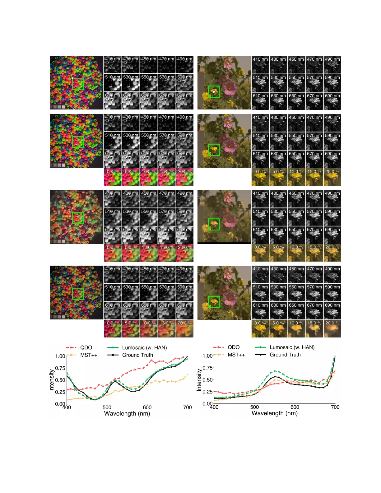
Lumosaic: Hyperspectral V ideo via Activ e Illumination and Coded-Exposure Pixels Dhruv V erma 1 Andre w Qiu 1 Roberto Rangel 2 A yandev Barman 2 Hao Y ang 2 Chenjia Hu 2 Fengqi Zhang 2 Roman Genov 2 David B. Lindell 1 Kiriakos N. K utulakos 1 Alex Mariakakis 1 1 Department of Computer Science, Uni versity of T oronto, Canada 2 Department of Electrical & Computer Engineering, Uni versity of T oronto, Canada dhruvverma@cs.toronto.edu A B C Figure 1. (A) Lumosaic is a compact acti ve hyperspectral video system that combines programmable narro wband illumination with pixel- wise coded exposure to jointly encode spatial, spectral, and temporal information within each video frame, enabling real-time capture at 30 fps. (B) Reconstructed frames of a rotating globe, rendered in sRGB, sho wing smooth temporal progression despite rapid motion. (C) Reconstructed spectral channels (400-700 nm, 10 nm intervals) from the highlighted frame. Abstract W e pr esent Lumosaic, a compact active hyperspectral video system designed for real-time capture of dynamic scenes. Our approac h combines a narr owband LED array with a coded-exposur e-pixel (CEP) camera capable of high-speed, per-pixel exposur e contr ol, enabling joint encoding of scene information acr oss space, time, and wavelength within each video frame. Unlike passive snapshot systems that divide light acr oss multiple spectral channels simultaneously and assume no motion during a frame’ s exposur e, Lumosaic actively synchr onizes illumination and pixel-wise exposur e, impr oving photon utilization and pr eserving spectral fidelity under motion. A learning-based r econstruction pipeline then reco vers 31-channel hyperspectr al (400–700 nm) video at 30 fps and VGA r esolution, pr oducing temporally coher ent and spectrally accur ate r econstructions. Experiments on synthetic and r eal data demonstrate that Lumosaic significantly impr oves reconstruction fidelity and temporal stability over existing snapshot hyperspectral imaging systems, enabling r obust hyperspectral video acr oss diverse materials and motion conditions. 1. Introduction Hyperspectral imaging (HSI) captures scene reflectance across many contiguous wa velength bands, re vealing spectral features in visible to con ventional RGB cameras. This rich spectral information underpins a wide range of applications such as material classification [ 40 ], physiological monitoring [ 23 ], and spectral relighting [ 17 ]. Despite decades of progress, deliv ering HSI at sufficiently high speeds to enable hyperspectral video remains a fundamental challenge due to trade-offs between spectral resolution, light efficienc y , and temporal sampling. 1 T raditional HSI systems rely on spatial or spectral scanning, in which different bands are sequentially captured using tunable filters, gratings, or moving optics. These approaches provide high spectral fidelity b ut require long acquisition times, making them impractical for dynamic scenes. Snapshot HSI methods, such as those using coded apertures (e.g., CASSI) [ 2 ], diffracti ve optical elements (DOEs) [ 4 ], or multispectral filter arrays (MSF As) [ 11 ], address this limitation by compressing spectral information into a single exposure through static optical encodings. Still, these designs suffer from sev ere light loss and ill-posed inv ersions that amplify noise and motion artifacts. Such issues are particularly salient when capturing hyperspectral video. Short exposure times result in fewer photons per band, and scene motion causes smearing or ghosting due to temporally misaligned spectral samples. One way to improve optical throughput is to shift spectral modulation from passive optics that attenuate or disperse light to the illumination itself. In this paradigm, the emitted spectrum is acti vely varied in time and/or space to encode wavelength information directly in the light rather than through optical filtering. Activ e hyperspectral systems have explored this principle using temporally multiplex ed narrowband light sources [ 28 , 34 ] or spectrally structured projection [ 18 , 32 ], offering programmable control ov er when and where different spectral bands illuminate the scene. Howe ver , most of these systems achiev e fine control along only a single dimension (e.g., high-speed spectral modulation with LEDs or spatial selectivity with projectors). In a system called Lumosaic (see Figure 1 ), we demonstrate that motion-robust hyperspectral video can be achiev ed by jointly encoding space, time, and spectra within each video frame. Lumosaic combines a narrowband LED array and a cutting-edge coded-exposur e-pixel (CEP) image sensor [ 13 , 24 , 35 , 38 ]. As the system rapidly c ycles through multiple LED activ ations, pixels are exposed in a time-varying mosaic pattern to create a dense spatio-spectr o-temporal encoding of the scene within a single video frame. Lumosaic’ s hardware acts as an optical encoder, while a software pipeline decodes the signal through spectral demosaicing, motion alignment via optical flo w , and a learning-based reconstruction stage that recov ers 31-channel hyperspectral video (400-700 nm) from coded video frames captured at 30 fps. Unlike prior systems that relied on b ulky , alignment-sensitiv e, and aberration-prone optics [ 10 , 22 , 33 ], our signal acquisition operates entirely in silicon, enabling compact and calibration-free deployment. Rather than filtering broadband lighting, Lumosaic’ s activ e approach allows each LED’ s narrowband output to contribute fully to the captured signal, thereby improving photon efficienc y under dynamic or low-light conditions. Our main technical contributions include: • Lumosaic, a nov el hyperspectral video system that lev erages time-varying illumination with pixel-wise coded-exposure to densely encode information across space, time, and wa velength. • A compact hardware prototype that integrates a CEP sensor with a narrowband LED array capable of modulating light at microsecond scales, enabling real-time capture of dynamic spectral phenomena at 30 fps. • A jointly designed illumination-exposure coding scheme and reconstruction pipeline that estimates accurate and temporally coherent hyperspectral video with 31 channels spanning 400-700 nm at VGA resolution ( 640 × 480 ). Through extensi ve experiments on both synthetic and real data, we demonstrate that Lumosaic achieves significant improv ements in reconstruction accuracy ov er state-of-the-art snapshot HSI approaches. W e sho wcase its performance across div erse scenes with varying spatial, spectral, and motion characteristics, marking a step toward general-purpose, motion-robust hyperspectral videography . 2. Related W ork Snapshot Hyperspectral Imaging. Ef forts to enable snapshot HSI hav e primarily focused on encoding spectral information optically in hardware, yielding compressed measurements that can be expanded via computational reconstruction. Early approaches such as CASSI [ 2 ] employed dispersiv e optics, coded apertures, and relay lenses to achiev e single-shot acquisition b ut at the expense of bulk y equipment, extensiv e calibration, and complex in version. Subsequent designs improved compactness yet introduced new limitations: prism-based systems [ 3 ] suf fer from chromatic distortion and spatial blur due to dispersion; printed color-dot masks [ 39 ] ha ve lo w optical throughput and ill-conditioned spectral responses; and MSF As [ 11 ] capture very little light due to absorptiv e filtering, attenuating effecti ve signal contribution under time-constrained scenarios such as motion and video. DOEs [ 4 , 20 , 30 ] and metasurface array approaches [ 8 , 25 ] offer high spectral diversity in miniature form factors but remain sensitive to fabrication imperfections, wa velength-dependent ef ficiency , and static spatial encoding that breaks under high-speed motion or noise. W ithout explicit temporal coding, any scene mov ement during exposure introduces spatial–spectral mixing that is difficult to disentangle during reconstruction. Recent work from Shi et al. [ 30 ] reports using a 400 ms exposure time under indoor illumination conditions. At such timescales, 2 these systems are suitable for static imaging, yet fundamentally ill-suited for dynamic or motion-robust hyperspectral video. Active Hyperspectral Imaging. In contrast, active HSI approaches lev erage programmable light sources to modulate spectral content temporally or spatially . This often improves the ef fective contribution of incoming light to useful signal—an adv antage particularly beneficial under time-constrained conditions such as hyperspectral video. A common strategy in volves sequentially cycling narrowband LEDs or laser diodes [ 12 , 28 , 34 ], synchronizing them with the sensor to interleave spectral measurements across time. While conceptually simple, this strategy struggles in dynamic scenes where motion between frames causes spectral misalignment and inconsistent reflectance recovery . V erma et al. [ 34 ] mitigated this limitation by exploiting a rolling-shutter camera to multiplex spectral information within a single exposure, b ut as with all row-wise schemes, fast motion still produces characteristic rolling-shutter distortions. Structured-light methods extend this idea by projecting spatially-coded spectral patterns onto the scene [ 18 , 19 , 31 , 32 ], enabling sparse sampling of spatio-spectral content across multiple illumination patterns. Howe ver , the need for multiple projection patterns and exposures to span the full spectral range restricts capture speed. For instance, Shin et al. [ 32 ] presented a system that achieved video capture at only 6.6 fps, which is inadequate for fast motion. More recently , Y u et al. [ 37 ] combined a high-speed event camera with a synchronized “sweeping-rainbow” illumination pattern, encoding spectral changes as asynchronous temporal ev ents to achieve high temporal resolution. Howe ver , their reliance on mechanically rotating optics limits compactness and robustness, and the moving spectral sweep introduces aliasing and misalignment for motion orthogonal to the scan. Coded-Exposure-Pixel Imaging. A new class of programmable sensors known as multi-tap, multi-buck et, or coded-exposure-pix el sensors [ 6 , 13 , 16 , 24 , 35 ] pushes the boundaries of con ventional imaging by enabling per-pix el exposure modulation directly in hardware, allowing dense spatio-temporal coding without external optical modulation. Modern implementations of this sensor architecture achiev e VGA spatial resolution with pixel-wise modulation rates exceeding 39 kHz [ 13 ], unlocking unprecedented flexibility for encoding scene dynamics. While coded-exposure imaging in general has been explored for motion deblurring [ 29 ], HDR imaging [ 26 ], and transient analysis [ 22 ], its potential for hyperspectral video remains largely untapped. The ability to embed high-speed temporal coding directly at the pixel Figure 2. The operation of a single pix el in a coded-exposure-pix el (CEP) camera. Each pixel alternates between two charge storage sites (Bucket 0 and Bucket 1) according to a binary e xposure code. During each sub-frame, only one bucket integrates incident light, enabling temporal multiplexing across the e xposure period. lev el presents a unique opportunity to pair with programmable illumination for joint spectral–temporal multiplexing. Lev eraging this capability , Lumosaic introduces a tightly inte grated coding scheme where time-varying spectral illumination and pixel-wise exposures are jointly tiled across the sensor in a dense mosaic. Combined with a learning-based reconstruction pipeline, Lumosaic achiev es real-time capture at 30 fps and motion-robust recovery of hyperspectral video, preserving both spatial detail and spectral fidelity . 3. Imaging F orward Model Lumosaic combines time-varying illumination with spatio-temporal exposure modulation to achie ve dense spatio-spectro-temporal coding within each video frame. This section describes the imaging principles, coding scheme, and measurement model underlying the system. 3.1. Coded-Exposure-Pixel Camera A CEP camera dif fers from a con ventional CMOS image sensor in two key features. First, each pixel of the CEP camera incorporates two charge-collection sites, or buc kets , enabling the segregation of photo-induced charge accumulation. Second, the exposure duration of each pixel within a video frame is di vided into smaller interv als called sub-frames . Each pixel includes a one-bit writable memory that facilitates programmable control ov er which buck et is activ e during each sub-frame. Figure 2 illustrates the operation of a CEP camera pixel and the corresponding integration process over sub-frames. Charge accumulation occurs at tw o dif ferent timescales: 1. Sub-frame level: The char ge collected at each sub-frame is accumulated and transferred to the active buck et based on each pixel’ s control signal, and 2. Frame le vel: The total charge accumulated across all sub-frames is integrated and read out for each b ucket. Programming a CEP camera in volv es specifying the number of sub-frames per video frame, the duration of 3 each sub-frame, and the state of each pixel’ s e xposure at each sub-frame. The exposure schedule is represented by a binary matrix C ∈ { 0 , 1 } P × S , where P is the number of pixels and S is the number of sub-frames per frame. Each entry C p,s specifies which b ucket is acti ve for a given pixel p and sub-frame s . 3.2. Time-V arying Spectral Illumination W e deliv er spectral modulation by using an array of L narrowband LEDs, each with a distinct spectral power distribution E l ( λ ) , where λ denotes wav elength. The illumination is varied in synchrony with the sub-frame exposure modulation of the CEP camera. W e define the illumination schedule using a binary matrix I ∈ { 0 , 1 } S × L , where I s,l = 1 indicates that LED l is active during sub-frame s . The s -th row i s, : ∈ { 0 , 1 } L thus specifies which LEDs are acti vated during the given sub-frame. The resulting spectral irradiance incident on the scene for a giv en sub-frame is I s ( λ ) = L X l =1 I s,l · E l ( λ ) . (1) This temporally varying illumination encodes spectral content directly into the exposure sequence. T ogether , the illumination matrix I and the exposure code matrix C form the basis for our measurement model. 3.3. Joint Illumination and Exposur e Coding T o enable dense and structured multiplexing, we design a coding scheme that synchronizes LED activ ations with pixel exposures across tightly packed neighborhoods on the sensor . As shown in Figure 3 (B), we cycle through L narrowband LEDs across S sub-frames while spatially tiling both illumination and exposure schedules across the sensor in a mosaic-lik e fashion. Pixels are grouped into T repeating tiles (e.g., a 4 × 4 pixel mosaic yields T = 16 tiles) with unique exposure schedules. W e define tile exposure and illumination codes as C tile ∈ { 0 , 1 } T × S , I tile ∈ { 0 , 1 } T × S × L . (2) Here, C tile [ t, s ] = 1 indicates that pixels in tile t are actively integrating light during sub-frame s , and I tile [ t, s, l ] = 1 specifies that LED l is turned on during sub-frame s for tile t . W e define a mapping function π : { 1 , . . . , P } → { 1 , . . . , T } (3) that assigns each pixel index p to its corresponding tile index π ( p ) . Using this mapping, each pixel inherits its exposure and illumination codes as C p,s = C tile [ π ( p ) , s ] , I p,s,l = I tile [ π ( p ) , s, l ] . (4) Thus, all pixels with the same tile index share the same illumination pattern, while adjacent pixels observe different wav elength bands at dif ferent times. Over S sub-frames, this coordinated scheme produces a temporally staggered spectral mosaic —a single video frame in which different spatial locations encode distinct spectral and temporal samples of the scene. 3.4. Measurement Model The goal of our measurement model is to represent each hyperspectral video frame as a matrix R ∈ R P × Λ , where each ro w r p ∈ R Λ describes the spectral reflectance at a pixel p according to Λ discrete wa velength bands. From Equation 1 , the time-varying illumination at sub- frame s and pix el p can be expressed in discrete form as I p,s = L X l =1 I p,s,l E l , (5) where E l ∈ R Λ denotes the spectral power distribution of LED l , and I p,s,l ∈ { 0 , 1 } specifies whether that LED is activ e for pixel p during sub-frame s according to its tile schedule. Giv en the camera’ s spectral sensitivity S ∈ R Λ , the effecti ve spectral sensing v ector is a p,s = S ⊙ I p,s , (6) where ⊙ denotes element-wise multiplication across the Λ wa velength bands. The photo-response for pixel p in sub- frame s is then y p,s = a ⊤ p,s r p = Λ X k =1 S k I p,s,k r p,k . (7) Although the CEP camera supports dual-buck et readout, we discard measurements from Bucket 0 and retain only the integration from Bucket 1 in our implementation. The total measured intensity at pixel p over a frame is obtained by summing all sub-frames in which it is activ e: Y p = S X s =1 C p,s y p,s + η p , (8) where C p,s ∈ { 0 , 1 } indicates whether pixel p integrates light during sub-frame s , and η p accounts for sensor noise and other residual errors. Stacking all pix el measurements into a vector Y ∈ R P and vectorizing the hyperspectral cube as x = vec( R ) ∈ R P Λ giv es the global forward model: Y = A x + η , (9) where A ∈ R P × P Λ encodes the combined effects of illumination modulation, exposure coding, and sensor spectral sensitivity . Each ro w of A represents the ef fecti ve spectral integration weights for one pixel aggregated over all activ e sub-frames. This linear model defines how spatial, spectral, and temporal information are jointly encoded in a single captured frame, forming the basis for our hyperspectral reconstruction pipeline. 4 … Pixe l - wise Exposure Schedul e Illum inatio n Schedul e Spati o - spectro - temporal Codi ng Sub - frame s A B CEP camera Acti ve Ill uminat ion Modul e Figure 3. (A) Lumosaic features a CEP camera synchronized with a programmable array of narrowband LEDs. (B) Each sub-frame is assigned a unique LED and spatial exposure mask, producing a dense spatio-spectro-temporal scene encoding within a single video frame. 3.5. Hardwar e Prototype Lumosaic consists of a custom activ e illumination module and a prototype CEP camera (see Figure 3 (A)). Active Illumination Module. The illumination module comprises 12 high-po wer narrowband LEDs (Lumileds Luxeon C), each cov ering a distinct portion of the visible spectrum with a full-width-at-half-maximum (FWHM) of approximately 20–30 nm. All LEDs are driven by a custom current driver capable of switching at frequencies exceeding 100 kHz. A microcontroller (Adafruit ESP32 Feather v2) generates digital control signals that synchronize LED activ ation with the CEP camera’ s sub-frame clock, achieving microsecond-lev el timing precision. CEP Camera. The prototype uses a VGA-resolution ( 640 × 480 ) CEP image sensor that supports per-pixel binary exposure modulation. The sensor operates at up to 12,500 sub-frames per second, allo wing rapid alternation of illumination states within a single video frame. In our implementation, each video frame comprises S = 158 sub-frames of 170 µs each, yielding a total integration period of ∼ 27 ms that is suitable for 30-fps video. An additional ∼ 6 ms of readout and synchronization overhead introduces dead time between consecutive frames, making this the primary factor limiting the achiev able frame rate to 30 fps rather than the exposure duty cycle itself. Synchronization and Control. LED activ ation and sensor exposure schedules are jointly programmed and triggered via hardware-le vel synchronization lines. Each LED’ s activ ation window is mapped to a contiguous sequence of sub-frames that share a common exposure pattern. T o compensate for variations in LED output power and the camera’ s spectral sensitivity , LEDs with lower radiance are allocated proportionally longer activ ation durations, ensuring balanced spectral energy delivery across the frame. No two LEDs are acti ve simultaneously to minimize crosstalk and improv e spectral separability . Calibration. W e perform a one-time calibration procedure to characterize (1) the spectral power distribution of the illumination module, (2) the spectral sensitivity of the CEP camera, and (3) the system’ s ov erall radiometric response. These measurements define the parameters of the imaging forward model while ensuring that reconstructed hyperspectral data is both radiometrically accurate and physically consistent with real-world measurements. Each of the 12 LEDs is sequentially activ ated so that its emission spectrum E l can be measured with a calibrated spectroradiometer (K onica Minolta CS-2000), providing an accurate spectral power distribution from 380–780 nm. The camera’ s spectral sensitivity S is measured using a monochromator (Image Engineering camSPECS XL) with 5-nm interference filters; the outputs are aggregated into 10-nm bins for alignment with the reconstruction model. T o ensure accurate radiometric scaling, we capture a Macbeth ColorChecker and jointly optimize LED-specific gains to equalize integrated intensity across channels, compensating for residual non-uniformities in LED brightness, optical coupling, and sensor response. W e use the resulting calibration parameters in both simulation and real-world reconstruction. Detailed procedures and plots are provided in Supplementary Section 1 . 4. Hyperspectral V ideo Reconstruction Giv en a coded measurement Y i corresponding to frame i , our goal is to reconstruct the underlying hyperspectral scene R i ∈ R P × Λ , where each pixel’ s spectral reflectance r p spans Λ = 31 wavelength bands. W e first demosaic Y i into a set of LED-specific sub-images { Y (1) i , Y (2) i , . . . , Y ( L ) i } , where L = 12 denotes the number of narro wband LEDs. Each Y ( l ) i aggregates pixels assigned to LED l according to the known illumination–exposure mosaic described in Section 3 . W e then perform bilinear interpolation to upsample each sub-image to the full spatial resolution of the sensor . Unlike with passive filter array systems, our sub-images correspond to dif ferent time interv als within the exposure 5 period, meaning the y may be spatially misaligned in scenes with motion. T o av oid artif acts during reconstruction, we incorporate a temporal alignment step beforehand. 4.1. T emporal Alignment of Spectral Channels Each LED-specific sub-image Y ( l ) i represents scene content captured under a distinct narrowband illumination. This fact violates the photometric consistency assumption underlying con ventional optical flow methods, making direct alignment between sub-images unreliable. T o address this, we perform temporal alignment by estimating motion across sub-images corresponding to the same LED in adjacent frames. W e designate the sub-image illuminated by the lime-coloured LED, Y ( lime ) i , as the temporal reference for frame i due to its central wa velength and mid-exposure timing. For each other LED l , we determine its relativ e position in the illumination schedule and pair its sub-image Y ( l ) i with a temporally adjacent frame. If l occurs before the lime LED in the illumination cycle, we pair it with Y ( l ) i +1 ; if it occurs after , we pair it with Y ( l ) i − 1 . Using these pairs, we estimate motion fields with the Real-Time Intermediate Flo w Estimation (RIFE) network [ 14 ], which predicts an interpolated frame at a specified timestamp. W e warp each sub-image Y ( l ) i to the reference time of Y ( lime ) i , producing the temporally aligned result ˆ Y ( l ) i . 4.2. Learning-based Reconstruction For each video frame i , the temporally aligned sub-images { ˆ Y (1) i , ˆ Y (2) i , . . . , ˆ Y ( L ) i } serve as input to a deep neural network that reconstructs the corresponding hyperspectral image R i with Λ = 31 spectral channels. Model Ar chitecture. W e adopt the Holistic Attention Network (HAN) [ 27 ] as our reconstruction backbone because of its demonstrated effecti veness in image restoration tasks. The network consists of 18 residual blocks organized into 10 residual groups, each with 128 feature channels. Channel attention with a reduction ratio of 16 is applied to enhance feature discrimination across spectral bands. The model takes as input a 66 × 64 × 12 tensor , corresponding to a spatial crop of the 12 demosaiced and temporally aligned LED sub-images. The model outputs a 66 × 64 × 33 hyperspectral cube covering 33 spectral bands from 380–780 nm as follows: • Channel 1: Aggregated ultraviolet bands (380–390 nm), • Channels 2–32: Consecuti ve 10 nm bins spanning the visible range (400–700 nm), • Channel 33: Aggregated near -infrared bands (710–780 nm). Extrapolated edge channels (1 and 33) are included during training to improve reconstruction near the spectral boundaries b ut are discarded at inference, leaving Channels 2–32 as the final output. W e reconstruct hyperspectral images corresponding to full frames in a patch-wise manner and merge them using a weighted aggregation strategy to ensure seamless spatial continuity . Additional details on model architecture, patch-wise reconstruction, and aggregation are pro vided in Supplementary Section 3 . T raining Setup. T o train the reconstruction model, we simulate the proposed imaging system’ s forward model using hyperspectral image datasets while incorporating sensor noise to closely emulate real capture conditions. W e add zero-mean Gaussian noise with a standard deviation uniformly sampled between 0% and 15% of the maximum signal intensity . For data augmentation, we extract random spatial patches from hyperspectral images and apply random horizontal and vertical flips. Since most public datasets provide spectral measurements only between 400–700 nm, we extend the range to 380–780 nm by mirroring the edge channels: the 420-nm and 410-nm bands approximate the ultraviolet (380–390 nm) region, while channels beyond 710 nm are mirrored from the 700-nm band. These extrapolated channels are used only during training to stabilize spectral boundary reconstruction and are omitted at inference. W e minimize the L 1 loss between the predicted and ground-truth hyperspectral cubes using the Adam optimizer with a learning rate of 1 × 10 − 4 and def ault β parameters. W e implement the model in PyT orch and train it with a batch size of 14 and gradient accumulation o ver two steps for memory efficiency . T raining for 50,000 iterations on an NVIDIA R TX A6000 GPU takes approximately 24 hours, and inference on a single 640 × 480 frame requires 4.7 s. 5. Experiments W e ev aluate Lumosaic across simulations and real-world captures, progressing from controlled static reconstructions to dynamic video demonstrations. 5.1. Simulations Setup. Since publicly av ailable hyperspectral video datasets are rare and small, our simulations focus on static scene reconstruction. W e simulate image formation under matched conditions on a unified corpus of three datasets: CA VE [ 36 ] (32 indoor scenes), KA UST [ 21 ] (409 indoor and outdoor scenes), and ARAD [ 1 ] (949 indoor and outdoor scenes). After resampling each hypers pectral cube to 31 uniformly-spaced channels between 400–700 nm at 10-nm intervals, we di vide the corpus into 80%-10%-10% 6 splits for training, validation, and testing, respecti vely . W e compare reconstruction performance across the fiv e configurations: (1) Lumosaic’ s forward model with HAN [ 27 ] as its reconstruction backbone; (2) Lumosaic with a MCAN [ 9 ] backbone; (3) Lumosaic with a SRNet [ 5 ] backbone; (4) QDO [ 20 ], an end-to-end optimized DOE-based snapshot HSI system; and (5) MST++ [ 7 ], a data-driv en RGB-to-hyperspectral reconstruction method. W e train all models from scratch using identical data splits, input normalization, and optimization schedules. W e ev aluate performance on the held-out test set using standard spatial and spectral quality metrics: peak signal-to-noise ratio (PSNR), structural similarity index (SSIM), mean absolute error (MAE), and spectral angle mapper (SAM). Higher PSNR/SSIM and lower MAE/SAM indicate better reconstruction quality . Noise Robustness. T o assess stability under photon-limited conditions typical in fast motion and video capture, we add Gaussian noise lev els of σ = { 0% , 5% , 10% , 15% , 20% } relativ e to the maximum signal intensity . As sho wn in Figure 4 , Lumosaic consistently achiev es higher SSIM and lower SAM compared to baselines across all noise lev els, while maintaining very high PSNR. Qualitativ e comparisons in Supplementary Section 4 show that Lumosaic preserves spatial details and accurate spectral reflectance, whereas QDO and MST++ exhibit noticeable blurring and spectral distortion under higher noise. Reconstruction Backbone Sensitivity . All three Lumosaic-based models spectrally outperform external baselines (QDO and MST++) while maintaining high spatial fidelity , highlighting the performance gains of our sensing model rather than mere network complexity . Among the reconstruction backbones, HAN deli vers the best fidelity , reaching 44.0 dB in the noise-free case and 32.0 dB ev en at σ = 20% (see Figure 4 ). MCAN and SRNet perform slightly worse than HAN in reconstruction accuracy but require significantly less compute and inference time (52 ms and 27 ms per frame, respecti vely), making them attractiv e for real-time deployment. Spectral Resolution. Supplementary Section 4.3 describes additional experiments on synthesized scenes to demonstrate Lumosaic’ s capability of recov ering narrowband spectral features. Results show accurate reconstruction of sharp spectral transitions, even beyond the physical sampling limits of our 12-channel LED illumination. 5.2. Real-W orld Evaluation Static Scenes. T o assess spectral and perceptual fidelity , we capture se veral static scenes: a ColorChecker , optical filters, and e veryday objects (e.g., fabrics, printed Figure 4. Reconstruction performance of QDO [ 20 ], MST++ [ 7 ], and Lumosaic using HAN [ 27 ], MCAN [ 9 ], and SRNet [ 5 ] backbones according to (top-left) PSNR, (top-right) MAE, (bottom-left) SSIM, and (bottom-right) SAM for the sim ulations under varying Gaussian noise le vels. B C D A Figure 5. Quantitative and qualitative ev aluation of spectral reconstruction accuracy using a ColorChecker target (real data). (A) Raw coded frame captured by Lumosaic. (B) Zoomed- in region showing the mosaic coding. (C) Reconstructed hyperspectral image rendered in sRGB. (D) Spectral reflectance curves for all 24 patches, comparing ground-truth (solid blue) and reconstructed (dashed yellow) spectra. materials, and figurines). As shown in Figure 5 , the reconstructed reflectance spectra from the ColorChecker closely match the ground truth from a spectroradiometer (K onica Minolta CS-2000), validating both the radiometric calibration and spectral reconstruction accuracy . Additional examples ( Figure 6 and 7 A B C Figure 6. An example of real-world reconstruction results obtained using Lumosaic. (A) Reconstructed hyperspectral image rendered as sRGB. (B) Reflectance spectra extracted from marked regions. (C) Reconstructed hyperspectral channels. Supplementary Section 5.1 ) show faithful color reconstruction and high perceptual consistency across div erse materials and textures. Metamerism Disambiguation. HSI can be used to discriminate between visually similar materials with different spectral properties. W e ev aluate Lumosaic’ s performance at this task by imaging a genuine, pigment-based ColorChecker and its printed photocopy . As sho wn in Supplementary Figure 10 , their reconstructed spectral reflectances differ significantly . Dynamic Scenes. Finally , we ev aluate Lumosaic on dynamic scenes exhibiting both rigid (translation, rotation, panning) and non-rigid (hand gestures, liquid diffusion, efferv escence) motions. Although millisecond-le vel of fsets between LED sub-images would typically induce motion blur , Lumosaic reconstructs temporally coherent hyperspectral video with high spectral fidelity and stability at 30 fps (see Figure 1 and 7 ). The Supplementary V ideo presents corresponding sRGB and hyperspectral renders, showing temporally stable reconstructions with minimal ghosting or flicker across all motion types. Additional results and ablations (Supplementary Section 5.3 and 5.4 ) highlight the contribution of our flow-based temporal alignment step in reducing motion-induced artifacts. 6. Future W ork & Concluding Remarks W e have demonstrated that Lumosaic can reconstruct 30-fps hyperspectral video at VGA resolution with 31 spectral channels (400-700 nm). This was made possible by coordinating time-varying illumination with a CEP Figure 7. Hyperspectral video reconstruction of a dynamic scene: a colored droplet diffusing in water , captured using Lumosaic at 30 fps. Each column shows a representative frame ov er time rendered in sRGB, while the bottom row visualizes reconstructed spectral channels for the highlighted frame. See the Supplementary V ideo for the full sequence visualization. camera to generate a dense spatio-spectro-temporal encoding within each video frame. Lumosaic’ s activ e, co-designed sensing strategy simultaneously acquires motion and spectral information with high light efficienc y—a capability not previously realized in such a compact form factor . Our results show temporally coherent and spectrally faithful reconstructions across div erse materials and motion patterns, bridging the long-standing gap between snapshot imaging and true hyperspectral video. There are numerous opportunities for future in vestigations. First, our reconstruction pipeline processes each frame independently , requiring us to push the limits of snapshot HSI to an acquisition speed suitable for video frame rates. Our main limiting factor was the dearth of comprehensiv e hyperspectral video datasets, which prev ented us from reliably training a network that could exchange information across consecuti ve frames. In future work, we will explore simulating motion in more widely av ailable hyperspectral image datasets to ov ercome this limitation. W e also did not fully le verage the CEP camera’ s affordances. Our implementation used only a single bucket of the underlying sensor . Since both buckets at each pixel integrate complementary illumination states over time, jointly modeling their responses could further improve dynamic range, light ef ficiency , and motion robustness. Finally , we did not fully e xplore the trade-of fs of different coding designs, as using adaptive or randomized mosaics may yield their own adv antages. In summary , Lumosaic establishes a new design space for computational hyperspectral video by coupling activ e 8 illumination with coded-exposure imaging. W e en vision this framework to enable new opportunities for real-time spectral sensing in robotics, microscopy , and computational photography . References [1] Boaz Arad, Radu T imofte, Ron y Y ahel, Nimrod Morag, Amir Bernat, Y uanhao Cai, Jing Lin, Zudi Lin, Haoqian W ang, Y ulun Zhang, Hanspeter Pfister , Luc V an Gool, Shuai Liu, Y ongqiang Li, Chaoyu Feng, Lei Lei, Jiaojiao Li, Songcheng Du, Chaoxiong W u, Y ihong Leng, Rui Song, Mingwei Zhang, Chongxing Song, Shuyi Zhao, Zhiqiang Lang, W ei W ei, Lei Zhang, Renwei Dian, Tianci Shan, Anjing Guo, Chengguo Feng, Jinyang Liu, Mirko Agarla, Simone Bianco, Marco Buzzelli, Luigi Celona, Raimondo Schettini, Jiang He, Y i Xiao, Jiajun Xiao, Qiangqiang Y uan, Jie Li, Liangpei Zhang, T aesung Kwon, Dohoon Ryu, Hyokyoung Bae, Hao-Hsiang Y ang, Hua-En Chang, Zhi-Kai Huang, W ei-Ting Chen, Sy-Y en Kuo, Junyu Chen, Haiwei Li, Song Liu, Sabarinathan, K Uma, B Sathya Bama, and S. Mohamed Mansoor Roomi. Ntire 2022 spectral recovery challenge and data set. In Pr oceedings of the IEEE/CVF Confer ence on Computer V ision and P attern Recognition (CVPR) W orkshops , pages 863–881, 2022. 6 , 4 [2] Gonzalo R Arce, David J Brady , Lawrence Carin, Henry Arguello, and David S Kittle. Compressiv e coded aperture spectral imaging: An introduction. IEEE Signal Pr ocessing Magazine , 31(1):105–115, 2013. 2 [3] Seung-Hwan Baek, Incheol Kim, Diego Gutierrez, and Min H Kim. Compact single-shot hyperspectral imaging using a prism. A CM T ransactions on Graphics (TOG) , 36 (6):1–12, 2017. 2 [4] Seung-Hwan Baek, Hayato Ikoma, Daniel S Jeon, Y uqi Li, W olfgang Heidrich, Gordon W etzstein, and Min H Kim. Single-shot hyperspectral-depth imaging with learned diffracti ve optics. In Pr oceedings of the IEEE/CVF International Confer ence on Computer V ision , pages 2651– 2660, 2021. 2 [5] Liheng Bian, Zhen W ang, Y uzhe Zhang, Lianjie Li, Y inuo Zhang, Chen Y ang, W en Fang, Jiajun Zhao, Chunli Zhu, Qinghao Meng, et al. A broadband hyperspectral image sensor with high spatio-temporal resolution. Nature , 635 (8037):73–81, 2024. 7 [6] Gil Bub, Matthias T ecza, Michiel Helmes, Peter Lee, and Peter Kohl. T emporal pixel multiplexing for simultaneous high-speed, high-resolution imaging. Nature methods , 7(3): 209–211, 2010. 3 [7] Y uanhao Cai, Jing Lin, Zudi Lin, Haoqian W ang, Y ulun Zhang, Hanspeter Pfister , Radu Timofte, and Luc V an Gool. Mst++: Multi-stage spectral-wise transformer for efficient spectral reconstruction. In Pr oceedings of the IEEE/CVF Confer ence on Computer V ision and P attern Recognition (CVPR) W orkshops , pages 745–755, 2022. 7 , 5 , 6 , 8 [8] MohammadSadegh Faraji-Dana, Ehsan Arbabi, Hyounghan Kwon, Seyedeh Mahsa Kamali, Amir Arbabi, John G Bartholomew , and Andrei Faraon. Hyperspectral imager with folded metasurface optics. Acs Photonics , 6(8):2161– 2167, 2019. 2 [9] Kai Feng, Y ongqiang Zhao, Jonathan Cheung-W ai Chan, Seong G Kong, Xun Zhang, and Binglu W ang. Mosaic con volution-attention network for demosaicing multispectral filter array images. IEEE T ransactions on Computational Imaging , 7:864–878, 2021. 7 [10] W ei Feng, Fumin Zhang, Xinghua Qu, and Shiwei Zheng. Per-pix el coded exposure for high-speed and high-resolution imaging using a digital micromirror de vice camera. Sensors , 16(3):331, 2016. 2 [11] Bert Geelen, Nicolaas T ack, and Andy Lambrechts. A compact snapshot multispectral imager with a monolithically integrated per -pixel filter mosaic. In Advanced fabrication technologies for micr o/nano optics and photonics VII , pages 80–87. SPIE, 2014. 2 [12] Mayank Goel, Eric Whitmire, Alex Mariakakis, T Scott Saponas, Neel Joshi, Dan Morris, Brian Guenter , Marcel Gavriliu, Gaetano Borriello, and Shwetak N Patel. Hypercam: hyperspectral imaging for ubiquitous computing applications. In Pr oceedings of the 2015 A CM International Joint Confer ence on P ervasive and Ubiquitous Computing , pages 145–156, 2015. 3 [13] Rahul Gulve, Navid Sarhangnejad, Gairik Dutta, Motasem Sakr , Don Nguyen, Roberto Rangel, W enzheng Chen, Zhengfan Xia, Mian W ei, Nikita Guse v , et al. 39 000- subexposures/s dual-adc cmos image sensor with dual- tap coded-exposure pixels for single-shot hdr and 3-d computational imaging. IEEE Journal of Solid-State Cir cuits , 58(11):3150–3163, 2023. 2 , 3 [14] Zhewei Huang, T ianyuan Zhang, W en Heng, Boxin Shi, and Shuchang Zhou. Real-time intermediate flow estimation for video frame interpolation. In Computer V ision – ECCV 2022: 17th Eur opean Conference, T el A viv , Israel, October 23–27, 2022, Pr oceedings, P art XIV , page 624–642, Berlin, Heidelberg, 2022. Springer -V erlag. 6 , 3 [15] Zhewei Huang, T ianyuan Zhang, W en Heng, Boxin Shi, and Shuchang Zhou. Real-time intermediate flo w estimation for video frame interpolation. https :/ /github . com/ hzwer/ECCV2022- RIFE , 2022. 3 [16] Jubin Kang, Y ongjae Park, Jung-Hye Hwang, Kieop Hong, Insang Son, Jung-Hoon Chun, Jaehyuk Choi, and Seong- Jin Kim. An indirect time-of-flight sensor with tetra-pixel architecture calibrating tap mismatch in a single frame. IEEE Solid-State Cir cuits Letters , 5:284–287, 2022. 3 [17] Chloe LeGendre, Xueming Y u, Dai Liu, Jay Busch, Andrew Jones, Sumanta Pattanaik, and Paul Debe vec. Practical multispectral lighting reproduction. ACM T ransactions on Graphics (T OG) , 35(4):1–11, 2016. 1 [18] Chunyu Li, Y usuke Monno, Hironori Hidaka, and Masatoshi Okutomi. Pro-cam ssfm: Projector-camera system for structure and spectral reflectance from motion. In Pr oceedings of the IEEE/CVF International Confer ence on Computer V ision , pages 2414–2423, 2019. 2 , 3 [19] Chunyu Li, Y usuke Monno, and Masatoshi Okutomi. Deep hyperspectral-depth reconstruction using single color -dot projection. In Proceedings of the IEEE/CVF Conference 9 on Computer V ision and P attern Recognition , pages 19770– 19779, 2022. 3 [20] Lingen Li, Lizhi W ang, W eitao Song, Lei Zhang, Zhiwei Xiong, and Hua Huang. Quantization-aware deep optics for diffracti ve snapshot hyperspectral imaging. In 2022 IEEE/CVF Conference on Computer V ision and P attern Recognition (CVPR) , pages 19748–19757, 2022. 2 , 7 , 5 , 6 , 8 [21] Y uqi Li, Qiang Fu, and W olfgang Heidrich. Dataset for multispectral illumination estimation using deep unrolling network, 2021. 6 , 4 [22] Dengyu Liu, Jinwei Gu, Y asunobu Hitomi, Mohit Gupta, T omoo Mitsunaga, and Shree K Nayar . Efficient space-time sampling with pixel-wise coded exposure for high-speed imaging. IEEE tr ansactions on pattern analysis and machine intelligence , 36(2):248–260, 2013. 2 , 3 [23] Guolan Lu and Baowei Fei. Medical hyperspectral imaging: a re view . Journal of biomedical optics , 19(1):010901– 010901, 2014. 1 [24] Y i Luo, Derek Ho, and Shahriar Mirabbasi. Exposure- programmable cmos pixel with selectiv e charge storage and code memory for computational imaging. IEEE T ransactions on Circuits and Systems I: Regular P apers , 65 (5):1555–1566, 2017. 2 , 3 [25] Maksim Makarenko, Arturo Bur guete-Lopez, Qizhou W ang, Fedor Getman, Silvio Giancola, Bernard Ghanem, and Andrea Fratalocchi. Real-time hyperspectral imaging in hardware via trained metasurface encoders. In Proceedings of the IEEE/CVF Conference on Computer V ision and P attern Recognition , pages 12692–12702, 2022. 2 [26] Julien NP Martel, Lorenz K Mueller, Stephen J Carey , Piotr Dudek, and Gordon W etzstein. Neural sensors: Learning pixel exposures for hdr imaging and video compressive sensing with programmable sensors. IEEE transactions on pattern analysis and mac hine intelligence , 42(7):1642–1653, 2020. 3 [27] Ben Niu, W eilei W en, W enqi Ren, Xiangde Zhang, Lianping Y ang, Shuzhen W ang, Kaihao Zhang, Xiaochun Cao, and Haifeng Shen. Single image super -resolution via a holistic attention network. In Computer V ision – ECCV 2020: 16th Eur opean Confer ence, Glasgow , UK, August 23–28, 2020, Pr oceedings, P art XII , page 191–207, Berlin, Heidelberg, 2020. Springer-V erlag. 6 , 7 , 3 [28] Jong-Il Park, Moon-Hyun Lee, Michael D Grossber g, and Shree K Nayar . Multispectral imaging using multiplexed illumination. In 2007 IEEE 11th International Confer ence on Computer V ision , pages 1–8. IEEE, 2007. 2 , 3 [29] Ramesh Raskar, Amit Agraw al, and Jack T umblin. Coded exposure photography: motion deblurring using fluttered shutter . In Acm Sig graph 2006 P apers , pages 795–804. 2006. 3 [30] Zheng Shi, Xiong Dun, Haoyu W ei, Siyu Dong, Zhanshan W ang, Xinbin Cheng, Felix Heide, and Y ifan Peng. Learned multi-aperture color-coded optics for snapshot h yperspectral imaging. ACM T ransactions on Graphics (TOG) , 43(6):1– 11, 2024. 2 [31] Suhyun Shin, Seokjun Choi, Felix Heide, and Seung-Hwan Baek. Dispersed structured light for hyperspectral 3d imaging. In Pr oceedings of the IEEE/CVF Conference on Computer V ision and P attern Recognition , pages 24997– 25006, 2024. 3 [32] Suhyun Shin, Seungwoo Y oon, Ryota Maeda, and Seung- Hwan Baek. Dense dispersed structured light for hyperspectral 3d imaging of dynamic scenes. arXiv preprint arXiv:2412.01140 , 2024. 2 , 3 [33] Edwin V argas, Julien NP Martel, Gordon W etzstein, and Henry Arguello. T ime-multiplex ed coded aperture imaging: Learned coded aperture and pix el exposures for compressi ve imaging systems. In Proceedings of the IEEE/CVF International Confer ence on Computer V ision , pages 2692– 2702, 2021. 2 [34] Dhruv V erma, Ian Ruffolo, Da vid B Lindell, Kiriakos N Kutulakos, and Alex Mariakakis. Chromaflash: Snapshot hyperspectral imaging using rolling shutter cameras. Pr oceedings of the ACM on Interactive, Mobile, W earable and Ubiquitous T echnologies , 8(3):1–31, 2024. 2 , 3 [35] Mian W ei, Navid Sarhangnejad, Zhengfan Xia, Nikita Gusev , Nikola Katic, Roman Genov , and Kiriakos N Kutulakos. Coded two-buck et cameras for computer vision. In Pr oceedings of the Eur opean Confer ence on Computer V ision (ECCV) , pages 54–71, 2018. 2 , 3 [36] Fumihito Y asuma, T omoo Mitsunaga, Daisuke Iso, and Shree K Nayar . Generalized assorted pixel camera: postcapture control of resolution, dynamic range, and spectrum. IEEE transactions on image pr ocessing , 19(9): 2241–2253, 2010. 6 , 4 [37] Bohan Y u, Jinxiu Liang, Zhuofeng W ang, Bin Fan, Art Subpa-asa, Boxin Shi, and Imari Sato. Active hyperspectral imaging using an event camera. In Pr oceedings of the Computer V ision and P attern Reco gnition Confer ence , pages 929–939, 2025. 3 [38] Jie Zhang, T ao Xiong, Trac T ran, Sang Chin, and Ralph Etienne-Cummings. Compact all-cmos spatiotemporal compressiv e sensing video camera with pixel-wise coded exposure. Optics expr ess , 24(8):9013–9024, 2016. 2 [39] Y uanyuan Zhao, Hui Guo, Zhan Ma, Xun Cao, T ao Y ue, and Xuemei Hu. Hyperspectral imaging with random printed mask. In Pr oceedings of the IEEE/CVF Confer ence on Computer V ision and P attern Recognition , pages 10149– 10157, 2019. 2 [40] Tiancheng Zhi, Bernardo R Pires, Martial Hebert, and Sriniv asa G Narasimhan. Multispectral imaging for fine- grained recognition of powders on complex backgrounds. In Pr oceedings of the IEEE/CVF Conference on Computer V ision and P attern Recognition , pages 8699–8708, 2019. 1 10 Lumosaic: Hyperspectral V ideo via Activ e Illumination and Coded-Exposure Pixels Supplementary Document T able of Contents 1. Imaging System Prototype 1 1.1 . Activ e Illumination Module . . . . . . . . . 1 1.2 . Coding Scheme Design . . . . . . . . . . . . 1 1.3 . Calibration . . . . . . . . . . . . . . . . . . 2 2. T emporal Alignment and Motion Compensation 2 3. Hyperspectral V ideo Frame Reconstruction 3 3.1 . Model Architecture . . . . . . . . . . . . . . 3 3.2 . Patch-wise Reconstruction . . . . . . . . . . 3 3.3 . Aggregation of Patch-wise Results . . . . . . 4 4. Additional Results: Simulations 4 4.1 . Additional Details . . . . . . . . . . . . . . 4 4.2 . Comparisons with Baselines . . . . . . . . . 4 4.3 . High-Frequency Spectral Recov ery T est . . . 7 5. Additional Results: Real W orld 9 5.1 . Static Scenes . . . . . . . . . . . . . . . . . 9 5.2 . Metamerism Analysis . . . . . . . . . . . . 9 5.3 . Dynamic Scenes . . . . . . . . . . . . . . . 9 5.4 . Ablation: Effect of T emporal Alignment . . . 9 1. Imaging System Prototype Lumosaic employs a custom-b uilt imaging platform that combines activ ely modulated LED illumination with a coded-exposure-pix el (CEP) camera to achieve dense spatio–spectro–temporal encoding suitable for hyperspectral video capture. This section details the system’ s hardware design, control strategy , and calibration procedure. 1.1. Active Illumination Module W e developed a custom high-speed illumination module to enable time-v arying spectral excitation synchronized with the CEP camera ( Figure 2 ). The module integrates 12 high-power narro wband LEDs (Lumileds Luxeon C series) with full-width-at-half-maximum (FWHM) spectral bandwidths of approximately 20–30 nm, spanning the visible range. The LEDs are controlled by a constant-current, high-speed switching driv er capable of switching at rates exceeding 100 kHz. The imaging system is orchestrated by an Adafruit ESP32 Feather v2 microcontroller , which generates digital control signals for both the illumination module and the CEP camera. A single microsecond-resolution clock drives Figure 2. The hardware schematic of Lumosaic’ s acti ve illumination module. The ESP32 microcontroller coordinates the LED driv er array and issues synchronization pulses to the CEP camera. all timing ev ents, ensuring sub-frame synchronization between light modulation and sensor exposure. In our implementation, each hyperspectral video frame consists of 158 sub-frames; each sub-frame is 150 µ s in duration, corresponding to a total exposure window of 23.7 ms. Because indi vidual LEDs differ in radiant po wer and the camera e xhibits w av elength-dependent sensiti vity , we non-uniformly allocate sub-frame counts per LED to approximately equalize the integrated spectral energy deliv ered per frame. LEDs with lower radiance recei ve proportionally more sub-frames (allocated consecutively), whereas brighter ones recei ve fewer . This adaptive exposure scheduling improv es both channel balance and spectral dynamic range. The allocation used in our experiments is summarized in T able 2 . 1.2. Coding Scheme Design Figure 3 illustrates the 3 × 4 spatial–spectral mosaic tile that we achieve by coordinating illumination with pixel exposures. The pattern is ex ecuted left-to-right from the top-left corner to the bottom-right. The mapping between LEDs and tile positions attempts to spectrally and temporally distribute LEDs with adjacent spectra in order 1 T able 2. The LED exposure allocation per video frame compensates for relativ e intensity variations across LEDs and camera spectral sensitivity . Each LED’s sub-frame activ ations occur contiguously within the frame. LED Name Relativ e Allocation Time per Frame (µs) UV 5.70% 1,350 V iolet 3.16% 750 Royal Blue 3.16% 750 Blue 3.16% 750 Cyan 5.70% 1,350 Green 6.96% 1,650 Lime 5.06% 1,200 Amber 25.32% 6,000 Red Orange 8.23% 1,950 Red 7.59% 1,800 Deep Red 6.96% 1,650 Far Red 18.99% 4,500 T otal 100.00% 23,700 Royal Blue Green Blue Far Red Cyan Red Lime Amber Red Orange Vio let Deep Red UV Figure 3. The 3 × 4 mosaic tile that forms the basis of Lumosaic’ s spatial-spectral coding. to minimize correlations between nearby measurements. 1.3. Calibration T o ensure accurate spectral recovery , we jointly calibrate LED intensity scaling factors and camera gain for each spectral channel. Calibration minimizes reconstruction error over ColorChecker measurements captured under controlled illumination. Measurements. W e first measure the spectral power distribution of each LED at a fixed position using a calibrated spectroradiometer (K onica Minolta CS-2000), yielding high-resolution emission profiles E l ( λ ) from 380–780 nm at 1-nm intervals. W e repeat this process for an incandescent bulb to generate an emission profile B ( λ ) . T o characterize the ColorChecker , we measure the spectral radiance of each patch C ′ p ( λ ) under illumination from the incandescent bulb using the same spectroradiometer . W e compute the spectral reflectance of each patch C p ( λ ) by dividing the measured radiance by the incident illumination: C p ( λ ) = C ′ p ( λ ) / B ( λ ) . (1) W e measure the camera’ s spectral sensitivity S ( λ ) using a monochromator (Image Engineering camSPECS XL) with 39 interference filters, producing calibrated spectral response curves at a resolution of 5 nm. These curves are quantized by spectral binning into Λ = 41 channels spanning 380–780 nm in 10-nm increments, resulting in spectral vectors E l ∈ R Λ , C p ∈ R Λ , and S ∈ R Λ . W e then capture five repeated measurements of the ColorChecker using Lumosaic and average them to reduce noise. The resulting image is then demosaiced to produce L = 12 sub-images, one for each LED. For each LED sub-image, we sample a region within each ColorChecker patch (total 24 patches) and compute the average intensity . This yields an empirical camera response matrix M real ∈ R L × 24 where each entry represents the a verage response of the camera to a specific LED and ColorChecker patch. Computing Calibration Coefficients. W e determine a vector of LED scaling factors α ∈ R L by simulating a theoretical camera response matrix M sim l,p from a simplified version of our image formation model: M sim l,p = Λ X λ =1 α l · ( E l ) λ · ( C p ) λ · S λ . (2) T o calculate α , we minimize the non-negati ve least-squares reconstruction error between α -scaled simulated intensities and our av eraged measurements on the ColorChecker: α = arg min α ≥ 0 X l,m ([ Λ X λ =1 α l · ( E l ) λ · ( C p ) λ · S λ ] − M real l,p ) 2 . (3) The optimized α l values are used to scale the LED emission curves, producing calibrated spectra E ′ l ( λ ) = α l E l ( λ ) used in all forward modeling and reconstruction experiments. 2. T emporal Alignment and Motion Compensation Because each sub-image corresponds to a distinct time interval within the total exposure window , scenes containing motion may exhibit spatial misalignment across spectral channels. T o prevent artifacts in hyperspectral reconstruction, we perform a temporal alignment step that warps all sub-images within a frame to a common temporal reference. Each sub-image Y l i in a gi ven frame i is assigned a timestamp according to its midpoint exposure timestamp. In other words, if Y l i is taken between t s l and t e l , we assign it a timestamp t l = ( t s l + t e l ) / 2 . The timestamps are normalized by the total duration of the frame, taking into 2 380 575 770 Wavelength (nm) 0.0 0.5 1.0 Intensity Uncalibrated Calibrated 380 575 770 Wavelength (nm) 0.0 0.5 1.0 Intensity Spectral Sensitivity Incandescent Bulb SPD Figure 4. (top) LED spectral power distributions before and after calibration via optimized scaling factors α λ . (bottom) Camera spectral sensitivity S ( λ ) and incandescent bulb spectral power distribution (SPD). account the CEP camera’ s 6 ms readout time, t readout : t ′ l = t l [ P l ( t e l − t s l )] + t readout . (4) This normalization pro vides a consistent temporal coordinate t ′ l ∈ [0 , 1] for ev ery sub-image, facilitating motion interpolation across time. W e use the Real-Time Intermediate Flow Estimation (RIFE) model [ 14 ] to estimate bidirectional flows between consecutiv e sub-images corresponding to the same LED across adjacent frames. RIFE jointly predicts interpolated flow fields and intermediate frames for arbitrary normalized timesteps t ′ ∈ [0 , 1] . W e specifically use RIFE v4.6 [ 15 ], which supports arbitrary-timestep warping and high-resolution inference. Using RIFE, we temporally align all sub-images in a frame to a common reference timestamp. W e select the lime-colored LED sub-image as the temporal reference because its illumination occurs near the frame’ s midpoint and its wav elength lies near the spectral center of the LED set. Suppose we are aligning the sub-image Y l i for any LED other than the lime-colored one. If LED l is scheduled before the reference ( t ′ l < t ′ lime ), we estimate the interpolated flow fields and warped image between its sub-image in the current frame Y l i and in the ne xt frame Y l i +1 . The normalized timestep t ′ provided to RIFE is determined by the distance between t ′ l and t ′ lime , t ′ = t ′ lime − t ′ l . If LED l is scheduled after the reference ( t ′ l > t ′ lime ), we use its sub-image in the previous frame Y l i − 1 and in the current frame Y l i , and the normalized timestep t ′ provided to RIFE is t ′ = (1 − t ′ l ) + t ′ lime . W e use the warped sub-images produced by RIFE as input to our downstream reconstruction model. 3. Hyperspectral V ideo Frame Reconstruction T o generate the full hyperspectral cube from each coded video frame, we apply hyperspectral reconstruction to the densely coded spectral mosaics. This section describes the reconstruction model and its application to the coded video frames. 3.1. Model Architectur e Our reconstruction network is based on the Holistic Attention Network (HAN) [ 27 ], which combines residual learning with hierarchical attention to model inter-channel correlations. The HAN architecture comprises multiple residual groups, each containing con volutional blocks enhanced by layer- and channel-lev el attention mechanisms. This design ef fectiv ely captures spatial context and spectral dependencies across the encoded mosaic. W e adapt HAN to our hyperspectral reconstruction setting with three key modifications: 1. W e adjust the first and final con volutional layers to handle our input of 12 LED sub-images and output of 33 spectral channels 1 . 2. Because our input and output share the same spatial resolution, we remove HAN’ s original upsampling module. 3. T o reduce GPU memory consumption and enable training on a single R TX A6000 or TIT AN R TX, we reduce the number of residual groups from 20 to 18. The final model contains approximately 57.1M trainable parameters. A detailed torchsummary -style architecture ov erview is sho wn in Figure 5 . 3.2. Patch-wise Reconstruction T o reduce GPU memory usage and enable efficient training, we reconstruct each frame in smaller ov erlapping patches. The demosaiced sub-images are partitioned into ov erlapping 66 × 64 × 12 patches using a sliding window with a stride of (30 , 32) and no padding. The stride ensures that the top-left corner of each patch aligns with the 3 × 4 spatial–spectral mosaic grid. When the windows do not completely cover the image, additional patches are appended along the right and bottom boundaries. The HAN network independently processes each patch to reconstruct its corresponding hyperspectral cube. This patch-wise approach allo ws large full-resolution frames to 1 T wo extrapolated boundary channels are included during training to improve reconstruction near spectral limits but are excluded from ev aluation. 3 Layer (type:depth-idx) Output Shape Param # --------------------------------------------------------------------------------- HANDSA [14, 33, 66, 64] -- UnshuffleToSpatiallyPreservingDemosaic: 1-1 [14, 12, 66, 64] -- PixelUnshuffle2D: 2-1 [14, 12, 22, 16] -- HAN: 1-2 [14, 33, 66, 64] -- Sequential: 2-2 [14, 128, 66, 64] -- Conv2d: 3-1 [14, 128, 66, 64] 13,952 Sequential: 2-3 -- -- ResidualGroup: 3-2 to 3-11 [14, 128, 66, 64] 54,999,200 Conv2d: 3-12 [14, 128, 66, 64] 147,584 LAM_Module: 2-4 [14, 1408, 66, 64] 1 Softmax: 3-13 [14, 11, 11] -- Conv2d: 2-5 [14, 128, 66, 64] 1,622,144 CSAM_Module: 2-6 [14, 128, 66, 64] 1 Conv3d: 3-14 [14, 1, 128, 66, 64] 28 Sigmoid: 3-15 [14, 1, 128, 66, 64] -- Conv2d: 2-7 [14, 128, 66, 64] 295,040 Sequential: 2-8 [14, 33, 66, 64] -- Conv2d: 3-16 [14, 33, 66, 64] 38,049 --------------------------------------------------------------------------------- Total params: 57,115,999 | Trainable: 57,115,999 | Non-trainable: 0 Total mult-adds (T): 3.35 Input size (MB): 9.94 | Fwd/bwd pass (MB): 22726.58 | Params (MB): 228.46 Estimated Total Size (MB): 22964.98 Figure 5. A summary of our modified HAN-based reconstruction model. 0 10 63 0 10 65 0 1 Weight Figure 6. A visualization of the spatial weighting k ernel K used for merging o verlapping patch predictions. be reconstructed without exceeding GPU memory limits while maintaining local spectral consistency across ov erlapping regions. 3.3. Aggregation of P atch-wise Results After reconstructing all patches, we reassemble them into the full-resolution hyperspectral frame using weighted av eraging to minimize boundary artifacts. Each reconstructed patch is multiplied by a predefined spatial weighting kernel K ∈ [0 , 1] 66 × 64 that assigns higher weights near the center and lo wer weights near the edges (see Figure 6 ). This spatial weighting mitigates discontinuities in ov erlapping regions. The final full-frame hyperspectral reconstruction is obtained as: R ′ = F old( K 66 × 64 × 33 ⊙ HAN(Unfold( Y ))) F old( K 66 × 64 × 33 ) , (5) where the ⊙ multiplication and the fractional di vision are applied element-wise. K 66 × 64 × 33 is the repetition of K in the spectral dimension. Unfold : R 640 × 480 → R L × 66 × 64 and F old : R L × 66 × 64 × 33 → R 640 × 480 × 33 are in verse-like sliding-window operations used to e xtract and reassemble the L overlapping patches, respectiv ely . HAN : R 66 × 64 → R 66 × 64 × 33 denotes the learned Holistic Attention Network used for patch-wise hyperspectral reconstruction. 4. Additional Results: Simulations 4.1. Additional Details During training, we extract random patches from each simulated measurement. T o ensure correct alignment between the illumination schedule and the pixel-wise coded-exposure pattern, the top-left corner of every patch is constrained to coincide with the top-left corner of a 3 × 4 mosaic tile (see Figure 3 ). This guarantees that ev ery extracted patch contains an integer number of complete mosaic repetitions and avoids boundary inconsistencies during reconstruction. Each batch is formed by sampling patches independently—potentially from dif ferent hyperspectral images—to improv e spectral div ersity and reduce overfitting. When noise robustness is ev aluated, we add independent Gaussian noise with standard de viation σ ∈ 0 , 5 , 10 , 15 , 20% of the maximum signal to each simulated patch before feeding it to the network. All corresponding hyperspectral ground-truth patches are extracted with identical spatial coordinates and normalized consistently . This pipeline ensures that the model learns reconstruction mappings that are faithful to the physical sensing process used in the real hardware. 4.2. Comparisons with Baselines Figure 7 presents qualitativ e comparisons of Lumosaic with a HAN backbone on test scenes from the CA VE [ 36 ], KA UST [ 21 ], and ARAD [ 1 ] datasets. Reconstructed 4 outputs from QDO [ 20 ] and MST++ [ 7 ] are provided as state-of-the-art comparisons. Across all the scenes presented, Lumosaic recovers finer spectral details and spatial textures while avoiding color bleeding commonly observed in the baselines. 5 Ground T ruth Full I mage Zoom ed - in Zoomed - in Full I mage Lumosaic (w. HAN) QDO MST++ Spectral Reflectance Figure 7. Qualitativ e comparisons on public datasets. Representative reconstructions from the test set comparing QDO [ 20 ], MST++ [ 7 ], and Lumosaic. Each column shows the reconstructed sRGB image, selected hyperspectral channels, and zoomed-in sRGB crops under varying Gaussian noise levels (annotated with the corresponding standard deviation). W e also present spectral v alidation plots for two specific locations, marked with white stars in the first-ro w sRGB images, displayed at the bottom of the figure. 6 4.3. High-Frequency Spectral Reco very T est W e assess Lumosaic’ s ability to recover high-frequency spectral features using a synthetic but deliberately challenging rainbow scene ( Figure 8 ). The scene is created by sweeping Gaussian-shaped spectral reflectance profiles with a FWHM of 20 nm 2 from the bottom to the top of a 512 × 512 image. The gradient spans the 400–700 nm range, so each ro w’ s central wavelength changes by (700-400 nm) / 512 px = 0.59 nm/px. Thus, adjacent rows differ only slightly in their peak wa velength, producing a high-frequency spectral gradient that stresses the model’ s ability to resolve fine spectral variations. This setup offers a controlled benchmark containing sharp spectral transitions that are rarely observed in natural scenes. As a result, it provides a practical out-of-distribution test of spectral resolving capability , rev ealing failure modes in con ventional snapshot systems that rely heavily on natural-scene priors and tend to oversmooth high-frequency spectra. As shown in Figure 8 (A-D), the baseline QDO [ 20 ] and MST++ [ 7 ] methods exhibit noticeable spectral smoothing and blending artifacts, failing to reproduce abrupt transitions between neighboring wa velength bands. In contrast, Lumosaic reconstructs these features while maintaining acceptable spatial fidelity and substantially better spectral localization across most of the gradient. This improv ement stems from its deterministic mosaic-based sensing strategy , which captures densely sampled, non-multiplexed spectral measurements rather than entangling multiple w avelengths within a single coded exposure. By reducing reliance on strong learned priors and providing cleaner spectral cues directly in the measurement domain, Lumosaic achiev es more accurate and reliable reconstruction of fine spectral structure. W e further analyze the influence of training data composition by introducing synthetic spectra that better represent narrow-band spectral features. The synthetic training data include two types of spectral vectors: 1. Single-peak pr ofiles: Gaussian functions are generated for center wa velengths from 400–700 nm with FWHM values of { 10, 20, 30, 40, 50 } nm. Each profile is sampled at 1-nm intervals, integrated into 10-nm bins using trapezoidal integration, and normalized to a maximum value of 1. 2. Double-peak pr ofiles: T wo Gaussian profiles are combined with center separations of { 10, 20, 30, 40, 60, 80 } nm, ensuring both peaks remain between 400 and 700 nm; the same integration and normalization procedure is applied. For training purposes, we use these synthetic spectra to create uniform, textureless hyperspectral images by 2 W e choose the narrowest FWHM supported by the LEDs used in our implementation. repeating each spectral vector spatially . W e compare versions of Lumosaic trained on 0%, 33%, 66%, and 100% synthetic spectra mixed with to natural scenes from our public dataset corpus, and and re-ev aluate them on the rainbow scene. As sho wn in Figure 8 (D-G), moderate synthetic augmentation (33%) provides the best trade-off between generalization and spectral precision, producing sharper and well-localized spectral peaks that closely align with the ground-truth spectra. Models trained exclusi vely on natural scenes exhibit lower sensitivity to subtle spectral variations, while heavier synthetic mixing (66% and 100%) offers limited additional resolving power and can slightly bias the reconstructions toward narrowband profiles. 7 Ground Trut h Reco nstruc ted Cent er Wav ele ngth A B C D E F G Figure 8. Spectral reco very test on a high-frequency rainbow scene. ( Left ) sRGB visualization of the rainbow scene: (A) ground truth and reconstructions from (B) QDO [ 20 ], (C) MST++ [ 7 ], and (D) Lumosaic. Rows (D-F) illustrate Lumosaic results under increasing proportions of high-frequency synthetic spectra in the training set (0%, 33%, 66%, 100%). ( Right ) Reconstructed spectral reflectance, interpolated at 1-nm intervals, and center wa velength positions at selected locations on the rainbo w (marked by triangles), compared to ground truth, demonstrating Lumosaic’ s improved ability to reco ver sharp spectral transitions. 8 5. Additional Results: Real W orld 5.1. Static Scenes Figure 9 further demonstrates Lumosaic’ s hyperspectral reconstruction capabilities for static scenes. As shown, Lumosaic correctly reconstructs fine-grained spatial details in each scene: the names of major countries and bodies of water on the globe, the box label and thin branches surrounding the butterfly , and the teeth of the figurine. The spectral information is also accurate, as clearly illustrated by the distinct colors of the countries on the globe. 5.2. Metamerism Analysis Figure 10 showcases Lumosaic’ s ability to resolve metameric ambiguities. Both targets appear visually identical under sRGB rendering, yet their spectral profiles differ notably across multiple patches. The genuine ColorChecker exhibits smooth, well-defined reflectance spectra characteristic of pigmented surfaces, whereas the printed copy sho ws irregular spectral peaks due to ink absorption and printer gamut limitations. 5.3. Dynamic Scenes Figure 11 and Figure 12 further demonstrate Lumosaic’ s capabilities as a hyperspectral video reconstruction system for dynamic scenes. In the scene with the rotating figurine ( Figure 11 , top), all printed elements, including the Ishihara pattern and the conference advertisement is properly resolv ed across the entire video, despite continuous rotational motion. In the hand gesture scene ( Figure 11 , bottom), there is some slight ghosting when the hand motion is fastest, but the content is nonetheless coherent. The scene with effervescent tonic water ( Figure 12 , top) is particularly well-suited for ev aluating hyperspectral video, as tonic water exhibits strong fluorescence for an otherwise transparent liquid. Despite the liquid’ s transparency , the system is able to render the bubbles with high spatial resolution. Finally , we demonstrate robustness to camera motion through a free-hand panning sequence ( Figure 12 , bottom), in which the system maintains stable hyperspectral reconstruction despite rapid viewpoint changes. 5.4. Ablation: Effect of T emporal Alignment W e assess the importance of our temporal alignment module by visualizing Lumosaic reconstructions with and without alignment at varying motion speeds. As shown in Figure 13 , fast-mo ving scenes exhibit ghosting and spectral blending artifacts when temporal alignment is not in use. These artifacts become increasingly pronounced at higher motion speeds, especially around edges or in areas with large brightness gradients. Applying temporal alignment produces sharper and more spectrally consistent outputs, confirming its crucial role in maintaining fidelity under motion. This is only made possible by the temporally coded illumination–exposure scheme underlying Lumosaic. Because each sub-frame captures a distinct wa velength band at a known temporal offset, our system inherently encodes both spectral and motion information within the same exposure sequence. The alignment module leverages this temporal structure to compensate for inter-frame motion, effecti vely restoring spatial–spectral coherence in dynamic scenes. 9 Butt erfl y Spe cime n Opti cal Filte rs Globe Figurine & Printed Matter A B C A B C A B C A B C Figure 9. Additional Lumosaic reconstruction results on diverse static scenes: optical filters, a globe, a butterfly specimen, and a figurine with printed matter . Each scene includes (A) the input coded image, (B) the reconstructed hyperspectral image rendered as sRGB, and (C) the 31-channel hyperspectral composites rendered in grayscale for visualization. 10 B C A Figure 10. Metamerism analysis with Lumosaic using genuine and printed ColorChecker targets. ( A and B ) RGB visualization of the genuine ColorChecker and a printed photocopy under identical illumination. ( C ) Spectral curves illustrating the differences between genuine and printed patches. 11 Hand Gestur es Figurine with Printed Matter Figure 11. Additional hyperspectral reconstruction results with Lumosaic on scenes exhibiting di verse motion characteristics. (top) A figurine with printed elements, including Ishihara patterns and text, undergoing both rotational and falling motion relati ve to the camera. (bottom) Dynamic hand gestures with non-rigid motion. The top row for each scene sho ws rendered sRGB vie ws from non-consecutive frames of the reconstructed hyperspectral video, while the bottom row shows the corresponding full 31-channel hyperspectral images for the frames outlined in yellow . 12 Free - hand Camer a Pa nning Effervescence Figure 12. Additional hyperspectral reconstruction results with Lumosaic on scenes exhibiting di verse motion characteristics. (top) A transparent plastic cup filled with carbonated tonic w ater, capturing high-frequency motion due to ef fervescence. (bottom) A complex indoor scene with colorful objects captured while freely panning the imaging system to introduce continuous viewpoint and illumination changes. The top ro w for each scene sho ws rendered sRGB vie ws sampled from non-consecuti ve frames of the reconstructed hyperspectral video, while the bottom row sho ws the corresponding full 31-channel hyperspectral images for the frames outlined in red. 13 Fast Slow With Alignment Without Alignment Without Alignment With Alignment Figure 13. The effect of temporal alignment on Lumosaic’ s reconstruction quality in dynamic scenes. W e compare results on two motion regimes— (top) slo w and (bottom) fast—showing hyperspectral reconstructions rendered in sRGB with and without temporal alignment. 14