Linear clique-width and modular decomposition

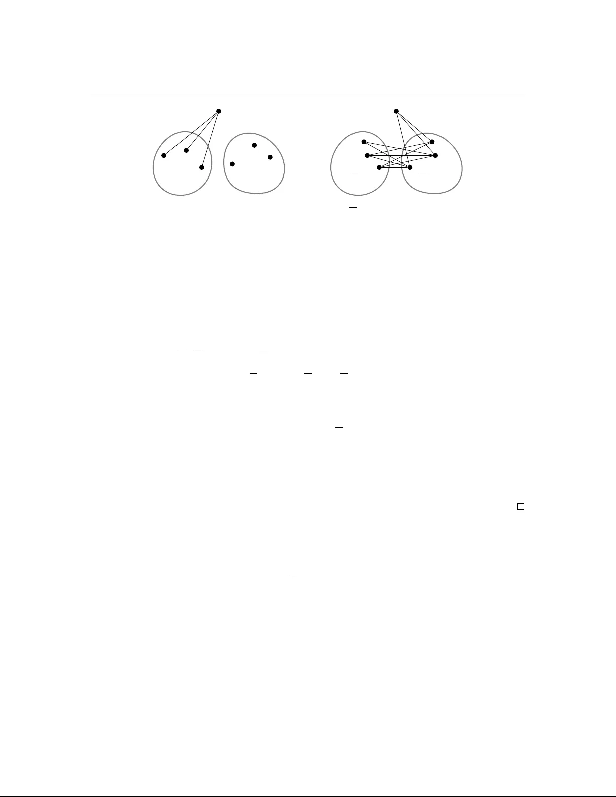
Linear Clique-Width and Modular Decomposition Rob ert Brignall ∗ , Mic hal Opler † , and Vincen t V atter ‡ F ebruary 26, 2026 A hereditary class of graphs has b ounded clique-width if and only if its prime mem b ers do, but this lifting prop ert y fails for linear clique-width. W e pro ve that a hereditary class has bounded linear clique-width if and only if its prime members do and it con tains neither all quasi-threshold graphs nor all complements of quasi-threshold graphs. This generalizes a result of Brignall, K orp elainen, and V atter, who established the result for cographs. 1. Intr oduction A hereditary class of graphs has b ounded clique-width if and only if its prime mem b ers ha v e b ounded clique-width; this follows easily from the definition. F or linear clique-width, how ev er, this lifting prop ert y fails. The class of cographs ( P 4 -free graphs) provides the simplest example: its only prime mem b ers, K 2 and K 2 , ha ve linear clique-width bounded b y 2 , yet the class itself has un b ounded linear clique-width. Brignall, K orp elainen, and V atter [8] identified the source of this failure within cographs, showing that the quasi-threshold graphs and their complements are the only obstructions. Theorem 1 .1 (Brignall, Korpelainen, and V atter [8, Theorem 1.1]) . A her e ditary class of c o gr aphs has b ounde d line ar clique-width if and only if it c ontains neither al l quasi-thr eshold gr aphs nor the c omplements of al l quasi-thr eshold gr aphs. Our main result shows that this is not sp ecial to cographs: quasi-threshold graphs and their com- plemen ts are, in general, the only obstructions to lifting b ounded linear clique-width from the prime mem b ers to the whole class. Theorem 1.2. A her e ditary class of gr aphs has b ounde d line ar clique-width if and only if its prime memb ers have b ounde d line ar clique-width and it c ontains neither al l quasi-thr eshold gr aphs nor al l c omplements of quasi-thr eshold gr aphs. ∗ The Op en Univ ersity , School of Mathematics and Statistics, Milton Keynes, England UK. † Czech T echnical Universit y , Departmen t of Theoretical Computer Science, Prague, Czech Republic. ‡ Universit y of Florida, Departmen t of Mathematics, Gainesville, Florida USA. 1 Linear Clique-Width and Modular Decomposition 2 There has b een considerable recent interest in identifying minimal hereditary classes of unbounded clique-width. Lozin [17] ga v e t w o examples of such classes, Collins, F oniok, K orp elainen, Lozin, and Zamaraev [10] found infinitely man y more, and Brignall and Co c ks [6] constructed uncoun tably many . A tminas, Brignall, Lozin, and Stacho [5] show ed that there exist minimal classes defined by finitely man y forbidden in duced subgraphs, disproving a conjecture of Daligault, Rao, and Thomassé [13], and in a separate work, Brignall and Co cks [7] dev elop ed a unifying framew ork encompassing nearly all known examples. As observed b y Alecu, Kanté, Lozin, and Zamaraev [4], many of these minimal classes are also minimal for linear clique-width, and this phenomenon recurs throughout the frame- w ork of [7]. Theorem 1.2 complemen ts this line of work: once one chec ks that a hereditary class excludes some quasi-threshold graph and some co-quasi-threshold graph, the question of whether the class has b ounded linear clique-wid th reduces entirely to its prime members. The pro of of Theorem 1.1 in [8] follow ed the blueprint of Alb ert, Atkinson, and V atter [2], who prov ed an analogous enumerativ e result for separable p erm utations. That blueprint inv olv es a substantial amoun t of well-quasi-order machinery whic h, while necessary to obtain the enumerativ e results in the p ermutation setting, is not needed for the graph-theoretic result. Indeed, this reliance on well- quasi-ordering was noted by Alecu, Kan té, Lozin, and Zamaraev [4], who commented that it limited the applicability of the approach. Our pro of of Theorem 1.2 is considerably more direct, requiring only mo dular decomp osition and explicit universal quasi-threshold graphs, and av oiding w ell-quasi- ordering entirely . 2. Linear Clique-Width and Universal Quasi-Threshold Graphs W e write G ⊎ H for the disjoint union of graphs G and H , and G ∗ H for their join , formed from G ⊎ H b y adding all edges with one endp oint in V ( G ) and the other in V ( H ) . W e write H ≤ G to mean that H is isomorphic to an induced subgraph of G . A set of graphs closed under isomorphism and closed down w ard under the induced subgraph order is called a her e ditary class , or simply a class . The line ar clique-width of a graph G , denoted lcw ( G ) , is the smallest num b er of lab els needed to construct G by a sequence of the following three op erations: • introduce a new v ertex and assign it a lab el, • for lab els i  = j , add edges b etw een all vertices lab eled i and all vertices lab eled j , and • for lab els i  = j , change the lab el of all v ertices lab eled i to j . Suc h a sequence is called an lcw expr ession for G , and an lcw expression is efficient if it uses exactly lcw( G ) lab els. A lab el in an lcw expression is a sink if it never app ears in an edge-creation or relab eling op eration; vertices ma y b e assigned to a sink lab el, but it is otherwise inert. Linear clique-width is a sequential restriction of clique-width . Clique-width was in tro duced by Cour- celle, Engelfriet, and Rozenberg [11], and it differs from linear clique-width in that clique-width expressions may additionally take the disjoint union of tw o previously constructed lab eled graphs. A closely related parameter, NLC-width , was introduced by W anke [20], and Gurski and W anke [16] w ere the first to study the linear v arian t of this family of parameters, under the name line ar NLC- width . Linear clique-width was subsequen tly int ro duced by Lozin and Rautenbac h [18]. W e consider the following families of graphs. A quasi-thr eshold gr aph (also called a trivial ly p erfe ct gr aph ) is any graph that can b e constructed from K 1 b y rep eatedly taking joins with K 1 , and disjoint unions with other quasi-threshold graphs; equiv alen tly , quasi-threshold graphs are the { P 4 , C 4 } -free Linear Clique-Width and Modular Decomposition 3 Q t − 1 Q t − 1 Q s − 1 Q s − 1 Figur e 1: The construction pro cess for the graphs Q t and Q s on the left and right, resp ectively . graphs. A c o-quasi-thr eshold gr aph is the complement of a quasi-threshold graph. A c o gr aph is any graph that can be constructed from K 1 b y rep eatedly taking disjoin t unions and joins; equiv alently , cographs are the P 4 -free graphs. Thus, the class of quasi-threshold graphs forms a prop er sub class of the class of cographs. W e now in tro duce graphs that are universal for the classes of quasi-threshold and co-quasi-threshold graphs. Our universal quasi-thr eshold gr aphs Q 1 , Q 2 , . . . are defined by Q 1 = K 1 and, for t ≥ 2 , Q t =  K 1 ∗ Q t − 1  ⊎ Q t − 1 . Their complements Q 1 , Q 2 , . . . satisfy Q 1 = K 1 and, for s ≥ 2 , Q s =  K 1 ⊎ Q s − 1  ∗ Q s − 1 . These graphs are depicted in Figure 1. Observ ation 2.1. F or every quasi-thr eshold gr aph G ther e exists t such that G ≤ Q t , and for every c o-quasi-thr eshold gr aph G ther e exists s such that G ≤ Q s . Pr o of. W e pro ve the first claim b y induction on | V ( G ) | ; the second follows by complementation. The base case is immediate since Q 1 = K 1 . Every quasi-threshold graph on t wo or more vertices is either a disjoint union G 1 ⊎ G 2 of smaller quasi-threshold graphs, or the join K 1 ∗ G ′ of a single v ertex with a smaller quasi-threshold graph. In the first case, G 1 , G 2 ≤ Q t − 1 b y induction, so G ≤ Q t − 1 ⊎ Q t − 1 ≤ Q t . In the second, G ′ ≤ Q t − 1 , so G ≤ K 1 ∗ Q t − 1 ≤ Q t . Ev ery cograph has clique-width at most 2 (this is immediate from the definitions and first observed b y Courcelle and Olariu [12]), but Gurski and W anke [16] show ed that this class has unbounded linear clique-width. Brignall, Korpelainen, and V atter [8] observed that linear clique-width is un b ounded ev en for the sub class of quasi-threshold graphs. Com bined with Observ ation 2.1, this implies that the linear clique-width of the graphs Q t and Q s is unbounded. 3. Modular Decomposition W e b egin by recalling the theory of mo dular decomp osition, which has b een indep endently disco v ered in numerous con texts; see Gallai [15, 19] for the foundational work in the graph setting. A mo dule of a graph G is a subset M ⊆ V ( G ) with the prop ert y that every vertex outside M is either adjacen t to all of the vertices of M or to none of them. The empty set, each singleton, and V ( G ) are all Linear Clique-Width and Modular Decomposition 4 mo dules; we call these trivial . A graph on at least tw o vertices is prime if all of its mo dules are trivial. Note that there are no prime graphs on three vertices, and that K 2 and K 2 are b oth prime under our definition; some other works require prime graphs to hav e at least four v ertices. Giv en a graph G , we say that G is an inflation of the graph H if G can b e obtained by replacing ev ery vertex v ∈ V ( H ) with a nonempty graph G v , so that ev ery vertex of G u is adjacent to every v ertex of G v in G if and only if u is adjacent to v in H . W e write this as G = H [ G v : v ∈ V ( H )] , and call H the skeleton of the decomp osition. Theorem 3.1. F or every gr aph G on two or mor e vertic es, ther e exists a unique prime gr aph H on two or mor e vertic es and nonempty gr aphs { G v : v ∈ V ( H ) } such that G = H [ G v : v ∈ V ( H )] . Mor e over, if H has at le ast four vertic es, then the gr aphs G v ar e also unique. When the skeleton provided by Theorem 3.1 has four or more vertices, it is neither complete nor an ti-complete, and the decomp osition is unambiguous. When the sk eleton is K 2 or K 2 , this means that either G or its complement, resp ectiv ely , is disconnected. In this case, we refine by decomp osing in to connected components or co-comp onents (connected comp onen ts of the complement), and take the skeleton to be an anti-complete or complete graph that is as large as p ossible. W e refer to the result of this pro cess as the first stage of the mo dular de c omp osition of G ; note that the full mo dular decomp osition would contin ue recursively to the mo dules, but we only need one stage at a time here. The remainder of this section establishes sev eral results relating linear clique-width to mo dular decomp osition. W e note that these results hold for arbitrary inflations, not only the unique inflations of prime graphs guaranteed by Theorem 3.1. The first has several pro ofs in the literature, including in Brignall, Korpelainen, and V atter [8, Prop osition 3.1]; w e pro vide another as it motiv ates the pro ofs that follow. Prop osition 3.2. If G = H [ { G v : v ∈ V ( H ) } ] , then lcw( G ) ≤ lcw( H ) + max v ∈ V ( H ) lcw( G v ) . Pr o of. Fix an efficient lcw expression for H . W e build an lcw expression for G by following the expression for H step b y step, replacing each vertex insertion with a construction of the en tire corresp onding mo dule: when the expression for H calls for the insertion of v ertex v with lab el ℓ , w e instead build a copy of G v using a set of lcw ( G v ) lab els reserved for mo dule constructions and disjoin t from those of the expression for H , then relab el every vertex of this copy to ℓ , and contin ue. Since the same reserved lab els are reused for each mo dule, the resulting expression uses at most lcw( H ) + max v ∈ V ( H ) lcw( G v ) lab els. When we are inflating a complete or anti-complete graph, we can slightly improv e up on the b ound of Prop osition 3.2. Prop osition 3.3. If G = H [ { G v : v ∈ V ( H ) } ] wher e H is c omplete or anti-c omplete, then lcw( G ) ≤ 1 + max v ∈ V ( H ) lcw( G v ) . Pr o of. Note that when H is anti-complete, this follows from Prop osition 3.2 since lcw ( H ) = 1 , but w e give a uniform argument cov ering b oth cases. W e reserve one lab el, ℓ , as a sink : a lab el that is nev er relab eled and never used in any edge-creation step except as describ ed b elow. W e then build Linear Clique-Width and Modular Decomposition 5 the mo dules G v one at a time, eac h using an efficient expression with lcw ( G v ) lab els, all distinct from ℓ . If H is complete, then after completing a mo dule G v , we join eac h of its lab els to ℓ (making its v ertices adjacent to the vertices of all previously completed modul es) and then relab el all of its v ertices to ℓ . If H is an ti-complete, we simply relab el all v ertices of G v to ℓ after completing it, without any join steps. In b oth cases, the resulting expression uses at most 1 + max v ∈ V ( H ) lcw( G v ) lab els. The following observ ation, whose pro of amoun ts to nothing more than giving a single vertex its own priv ate lab el, allows us to reorder the construction of a graph at the cost of that additional lab el. W e use it in the subsequent prop osition, where we are interested in bounding the linear clique-width of the tw o mo dules whose linear clique-width is largest. Prop osition 3.4. F or every gr aph G and every vertex v ∈ V ( G ) , ther e is an lcw expr ession of G with at most lcw( G ) + 1 lab els that b e gins by inserting the vertex v . Pr o of. Fix an efficien t lcw expression for G and let ℓ b e a new lab el not used in that expression. W e build G by first inserting v with lab el ℓ , and then following the original expression step by step with the following mo difications. W e skip the insertion of v when it arises. Whenev er the original expression relab els the lab el that v would hold at that p oint, we do not apply this relab eling to v (it retains the lab el ℓ throughout). Whenever the original expression creates edges b et ween the lab el that v would hold at that p oin t and some other lab el, w e additionally create edges b etw een ℓ and that lab el. This pro duces the same graph using at most one additional lab el, namely , ℓ . Com bining Prop ositions 3.2 and 3.4, we obtain the following result. Prop osition 3.5. Supp ose that G = H [ G v : v ∈ V ( H )] wher e H has at le ast two vertic es. Then either ther e is a vertex x of H for which lcw( G x ) = lcw ( G ) , or ther e ar e distinct vertic es x and y of H for which lcw( G x ) , lcw ( G y ) ≥ lcw ( G ) − lcw( H ) − 1 . Pr o of. Choose x ∈ V ( H ) to maximize lcw ( G x ) . By Prop osition 3.4, there is an expression for H using at most lcw( H ) + 1 lab els in which the v ertex x is inserted first. F ollowing the proof of Prop osition 3.2, we use this expression to build G : we first construct G x using lcw( G x ) lab els, then relab el all of its vertices to the lab el assigned to x in the expression for H , and contin ue following the expression for H , building each subsequent mo dule using the same lcw ( G x ) lab els. The construction of G x uses lcw ( G x ) lab els, while the remainder of the construction uses at most 1 + lcw ( H ) + max v  = x lcw( G v ) lab els. Since this is an lcw expression for G , one of these tw o quantities must b e at least lcw( G ) . If the first is, then we hav e lcw( G x ) = lcw ( G ) . Otherwise, choosing y ∈ V ( H ) \ { x } to maximize lcw( G y ) , w e obtain lcw( G y ) ≥ lcw ( G ) − lcw ( H ) − 1 , and lcw ( G x ) ≥ lcw ( G y ) b y our choice of x . Linear Clique-Width and Modular Decomposition 6 4. Pr oof of Theorem 1.2 Our main result follo ws from the following result, whic h can b e considered as a more precise version of Observ ation 2.1. Indeed, Prop osition 4.1 sho ws that any graph in a hereditary class satisfying the h yp otheses of Theorem 1.2 has linear clique-width b ounded by a function of m , t , and s , where m b ounds the linear clique-width of the prime members, and Q t and Q s are the first universal quasi- threshold and co-quasi-threshold graphs not in the class. Conv ersely , if a hereditary class contains all quasi-threshold graphs, then by Observ ation 2.1 it contains all Q t , so its linear clique-width is un b ounded, and likewise if it con tains all co-quasi-threshold graphs. The idea of the proof is as follows. Given a graph G of large linear clique-width, the mo dular decomp osition pro duces a skeleton H (of bounded linear clique-width) and mo dules whose linear clique-width is gov erned by Prop osition 3.5: that is, either one mo dule matches the linear clique- width of G (in whic h case w e apply induction) or tw o of them hav e large linear clique-width. If H is prime, there exist vertices with mixed adjacencies to these large mo dules, whic h directly yield the joins and disjoint unions needed to build Q t or Q s . If instead H is complete or an ti-complete, then G provides only one of these tw o op erations. W e then apply the mo dular decomp osition a second time to the mo dule of largest linear clique-width, which is forced to hav e the “opp osite” type of sk eleton, and find what we need at this second level. Prop osition 4.1. L et G b e a gr aph for which the line ar clique-width of every prime induc e d sub gr aph is at most m , and let t, s ≥ 1 . If lcw( G ) ≥ ( m + 2)( t + s ) , then G c ontains Q t or Q s as an induc e d sub gr aph. Pr o of. W e pro ceed by induction on the num b er of v ertices of G . W e may assume that m ≥ 2 , as otherwise G cannot contain K 2 , so G is anti-complete and cannot satisfy the b ound in the prop osition for any t, s ≥ 1 . In particular, G has at least tw o vertices, establishing the base case of our induction. W e may also assume that t, s ≥ 3 . Cases with t = 1 or s = 1 are trivial, since Q 1 = Q 1 = K 1 is an induced subgraph of ev ery nonempty graph. F or t = 2 , note that a graph not containing Q 2 = K 2 ⊎ K 1 as an induced subgraph is complete multipartite, with linear clique-width at most 2 . Since m ≥ 2 and s ≥ 1 , we hav e ( m + 2)(2 + s ) ≥ 12 > 2 , so every graph satisfying the b ound con tains Q 2 ≤ Q t . Dually , a graph not containing Q 2 = P 3 is a disjoin t union of cliques, with linear clique-width at most 3 . Since m ≥ 2 and t ≥ 1 , we hav e ( m + 2)( t + 2) ≥ 12 > 3 , so every graph satisfying our bound also contains Q 2 ≤ Q s . W e make this reduction b ecause t, s ≥ 3 ensures that Q t − 1 is disconnected and Q s − 1 is connected, prop erties we use in the argument b elow. No w supp ose that G satisfies the h yp otheses of the prop osition with m ≥ 2 and t, s ≥ 3 and that the result holds for all graphs with fewer v ertices. Apply the first stage of the mo dular decomp osition to write G = H [ G v : v ∈ V ( H )] where H is complete, anti-complete, or prime on at least four vertices, and in the first tw o cases the mo dules G v are the co-comp onents or connected comp onen ts of G , resp ectively . Let x b e a vertex of H for whic h lcw ( G x ) is maximal amongst all modules G v . If lcw ( G x ) = lcw ( G ) , then we are done b y induction b ecause G x itself satisfies the hypotheses and therefore con tains either Q t or Q s . Otherwise, Prop osition 3.5 provides a vertex y  = x of H suc h that lcw( G x ) , lcw ( G y ) ≥ lcw ( G ) − lcw( H ) − 1 . Linear Clique-Width and Modular Decomposition 7 Since lcw ( H ) ≤ m (as H is an induced subgraph of G that is either complete, anti-complete, or prime), we hav e lcw( G x ) , lcw ( G y ) ≥ lcw ( G ) − m − 1 ≥ ( m + 2)( t + s − 1) + 1 . Since G x and G y ha ve fewer vertices than G , the inductiv e hypothesis applies to them for all v alues of t and s . Applying it with ( t − 1 , s ) and ( t, s − 1) , w e conclude that each of G x and G y con tains Q t − 1 or Q s , and each also contains Q t or Q s − 1 . If either contains Q t or Q s , then so do es G and we are done. W e may therefore assume that b oth G x and G y con tain Q t − 1 and Q s − 1 . First s uppose that H is prime on four or more vertices. Because { x, y } do es not form a mo dule in H , there is some vertex z ∈ V ( H ) adjacent to precisely one of x or y . If x and y are adjacent in H , then G contains Q s = ( K 1 ⊎ Q s − 1 ) ∗ Q s − 1 , while if x and y are nonadjacent in H , then G con tains Q t = ( K 1 ∗ Q t − 1 ) ⊎ Q t − 1 , and in either case we are done. It remains to consider the case where H is complete or anti-complete. W e treat the anti-complete case first, and then explain the mo difications needed for the complete case. Supp ose that H is an ti-complete, so G is the disjoint union of its connected comp onents, t w o of whic h are G x and G y . By Prop osition 3.3, lcw ( G x ) ≥ lcw ( G ) − 1 ≥ ( m + 2)( t + s ) − 1 . Since G x is connected, its skeleton is either complete or prime on at least four vertices. If G x is the inflation of a complete graph (a join of co-comp onents), then since Q t − 1 is disconnected, it lies entirely within a single co-comp onent of G x , and any vertex from another co-comp onent is adjacen t to all of Q t − 1 . Thus G x con tains K 1 ∗ Q t − 1 , which together with the copy of Q t − 1 in G y giv es Q t = ( K 1 ∗ Q t − 1 ) ⊎ Q t − 1 in G . If G x is the inflation of a prime graph H ′ on four or more vertices, we apply Prop osition 3.5 to G x . Let a b e a vertex of H ′ maximizing lcw ( G ′ a ) . If lcw ( G ′ a ) = lcw ( G x ) , then G ′ a has fewer vertices than G and satisfies the hypotheses of the prop osition, so we are done by induction. Otherwise, Prop osition 3.5 provides a v ertex b  = a of H ′ with lcw( G ′ a ) , lcw ( G ′ b ) ≥ lcw ( G x ) − m − 1 ≥ ( m + 2)( t + s − 1) . Applying the inductive h yp othesis to G ′ a and G ′ b as we did with G x and G y earlier, we ma y assume that they each contain Q t − 1 and Q s − 1 . Since H ′ is prime, { a, b } is not a mo dule, so there exists a vertex c ∈ V ( H ′ ) adjacent to precisely one of a or b . Say c is adjacen t to a . Any v ertex of G ′ c is then adjacent to all of Q t − 1 inside G ′ a , giving a copy of K 1 ∗ Q t − 1 inside G x . Com bined with the cop y of Q t − 1 in G y (a separate comp onent of G ), we obtain Q t = ( K 1 ∗ Q t − 1 ) ⊎ Q t − 1 in G , completing the pro of in this case. No w supp ose that H is complete, so G is the join of its co-comp onents, tw o of which are G x and G y . By Prop osition 3.3, lcw ( G x ) ≥ ( m + 2)( t + s ) − 1 as b efore. Since G x is co-connected, its sk eleton is either anti-complete or prime on at least four v ertices. If G x is the inflation of an anti-complete graph (a disjoint union of connected comp onents), then Q s − 1 is connected (since s ≥ 3 ), so it lies within a single comp onen t of G x , and any v ertex from another comp onent is nonadjacent to all of Q s − 1 . Thus G x con tains K 1 ⊎ Q s − 1 , which together with the copy of Q s − 1 in G y (joined to G x since H is complete) gives Q s = ( K 1 ⊎ Q s − 1 ) ∗ Q s − 1 in G . If instead G x has a prime skeleton, we find tw o large mo dules inside G x eac h containing Q t − 1 and Q s − 1 , exactly as in the an ti-complete case. The prime skeleton of G x again provides a vertex c adjacent to precisely one of them, say c is adjacent to a but not to b . A vertex of G ′ c is then nonadjacent to all of Q s − 1 inside G ′ b , giving K 1 ⊎ Q s − 1 inside G x . T ogether with the copy of Q s − 1 in G y (joined to G x since H is complete), we obtain Q s = ( K 1 ⊎ Q s − 1 ) ∗ Q s − 1 in G . This completes the pro of. Linear Clique-Width and Modular Decomposition 8 W e do not claim that the b ound ( m + 2)( t + s ) in Prop osition 4.1 is optimal, although there is no slac k in the induction. The linear dep endence on t + s is correct, since lcw( Q t ) itself grows linearly in t . 5. Concluding Remarks Theorem 1.2 sho ws that the quasi-threshold graphs and their complements are the only obstructions to lifting bounded linear clique-width from the prime mem b ers to the whole class. F erguson and V atter [14, Theorem 5.1] prov ed an analogous result for lettericity , another graph width parameter: when the prime mem b ers of a class hav e b ounded lettericity , the class has b ounded lettericit y if and only if it excludes all matchings, all co-matchings, and all “stack ed paths”. More broadly , b oth results are instances of a familiar theme across com binatorics: if the “atoms” of a decomp osition are controlled, then unbounded complexity can only arise from a self-embedding mec hanism. The universal quasi-threshold graphs exhibit this concretely , as eac h Q t con tains tw o induced copies of Q t − 1 with one of the copies joined with K 1 to distinguish it. Complete binary trees pro vide another example: each is built by joining tw o copies of a smaller tree through a common ro ot, driving linear clique-width to infinity . (Binary trees do not contradict Theorem 1.2, b ecause the self-em b edding here o ccurs within the prime induced subgraphs themselv es, which ha ve unbounded linear clique-width.) The same moral underlies the excluded grid theorem, which identifies large grid minors as the canonical self-similar obstruction to b ounded treewidth, and the classical result of Chomsky and Sch ützen b erger [9] that a context-free grammar with no recursiv e nonterminals generates a regular language. The connection to p ermutation patterns is worth elab orating. The result of Brignall, Korpelainen, and V atter [8] that w e generalize here was itself the graph-theoretic analogue of the en umerativ e results of Alb ert, A tkinson, and V atter [2] for separable p erm utations. In that translation, cographs corresp ond to separable p ermutations, quasi-threshold and co-quasi-threshold graphs corresp ond to the classes Av(132) , Av (213) , Av(231) , and Av(312) , and modular decomp osition corresp onds to substitution decomp osition. Alb ert, A tkinson, and V atter show ed that a sub class of the separable p erm utations av oiding one of these four classes has a rational generating function, while our The- orem 1.2 extends the graph side of this analogy b eyond cographs to arbitrary hereditary classes whose prime graphs ha ve b ounded linear clique-width. Our results here suggest it may b e p ossible to extend the results of Alb ert, Atkinson, and V atter [2] to the con text of inflations of geometric grid classes [1, 3]. A c kno wledgemen ts. This research w as conducted at the Ob erwolfac h Mini-W orkshop on Perm u- tation Patterns, #2405c, held January 28–F ebruary 2, 2024. References [1] Alber t, M. H., A tkinson, M. D., Bouvel, M., Ruškuc, N., and V a tter, V. Geometric grid classes of p ermutations. T r ans. Amer. Math. So c. 365 , 11 (2013), 5859–5881. [2] Alber t, M. H., A tkinson, M. D., and V a tter, V. Sub classes of the separable p ermuta- tions. Bul l. L ond. Math. So c. 43 , 5 (2011), 859–870. [3] Alber t, M. H., Ruškuc, N., and V a tter, V. Inflations of geometric grid classes of p ermu- tations. Isr ael J. Math. 205 , 1 (2015), 73–108. Linear Clique-Width and Modular Decomposition 9 [4] Alecu, B., Kanté, M. M., Lozin, V., and Zamaraev, V. Betw een clique-width and linear clique-width of bipartite graphs. Discr ete Math. 343 , 8 (2020), Article 111926, 14 pp. [5] A tminas, A., Brignall, R., Lozin, V., and St acho, J. Minimal classes of graphs of un b ounded clique-width defined by finitely many forbidden induced subgraphs. Discr ete Appl. Math. 295 (2021), 57–69. [6] Brignall, R., and Cocks, D. Uncountably many minimal hereditary classes of graphs of un b ounded clique-width. Ele ctr on. J. Combin. 29 , 1 (2022), P ap er No. 1.63, 27 pp. [7] Brignall, R., and Cocks, D. A framework for minimal hereditary classes of graphs of un b ounded clique-width. SIAM J. Discr ete Math. 37 , 4 (2023), 2558–2584. [8] Brignall, R., Korpelainen, N., and V a tter, V. Linear clique-width for hereditary classes of cographs. J. Gr aph The ory 84 (2017), 501–511. [9] Chomsky, N., and Schützenberger, M. P. The algebraic theory of con text-free languages. In Computer pr o gr amming and formal systems . North-Holland, Amsterdam, The Netherlands, 1963, pp. 118–161. [10] Collins, A., Foniok, J., Korpelainen, N., Lozin, V., and Zamaraev, V. Infinitely man y minimal classes of graphs of unbounded clique-width. Discr ete Appl. Math. 248 (2018), 145–152. [11] Cour celle, B., Engelfriet, J., and Rozenber g, G. Handle-rewriting hypergraph gram- mars. J. Comput. System Sci. 46 , 2 (1993), 218–270. [12] Cour celle, B., and Olariu, S. Upp er b ounds to the clique width of graphs. Discr ete Appl. Math. 101 , 1-3 (2000), 77–114. [13] D aliga ul t, J., Rao, M., and Thomassé, S. W ell-quasi-order of relab el functions. Or der 27 , 3 (2010), 301–315. [14] Fer guson, R., and V a tter, V. Letter graphs and mo dular decomp osition. Discr ete Appl. Math. 309 (2022), 215–220. [15] Gallai, T. T ransitiv orientierbare Graphen. A cta Math. A c ad. Sci. Hungar. 18 , 1-2 (1967), 25–66. [16] Gurski, F., and W anke, E. On the relationship b etw een NLC-width and linear NLC-width. The or et. Comput. Sci. 347 , 1-2 (2005), 76–89. [17] Lozin, V. Minimal classes of graphs of un bounded clique-width. Ann. Comb. 15 , 4 (2011), 707–722. [18] Lozin, V., and Rautenba ch, D. The relative clique-width of a graph. J. Combin. The ory Ser. B 97 , 5 (2007), 846–858. [19] Maffra y, F., and Preissmann, M. A translation of Gallai’s paper: “ Transitiv orien tierbare Graphen”. In Perfe ct Gr aphs , J. L. Ramírez Alfonsín and B. A. Reed, Ed s., vol. 44 of Wiley Series in Discr ete Math. & Optim. Wiley , Chic hester, England, 2001, pp. 25–66. [20] W anke, E. k -NLC graphs and p olynomial algorithms. Discr ete Appl. Math. 54 , 2-3 (1994), 251–266.