Spin chains for ADE quiver theories

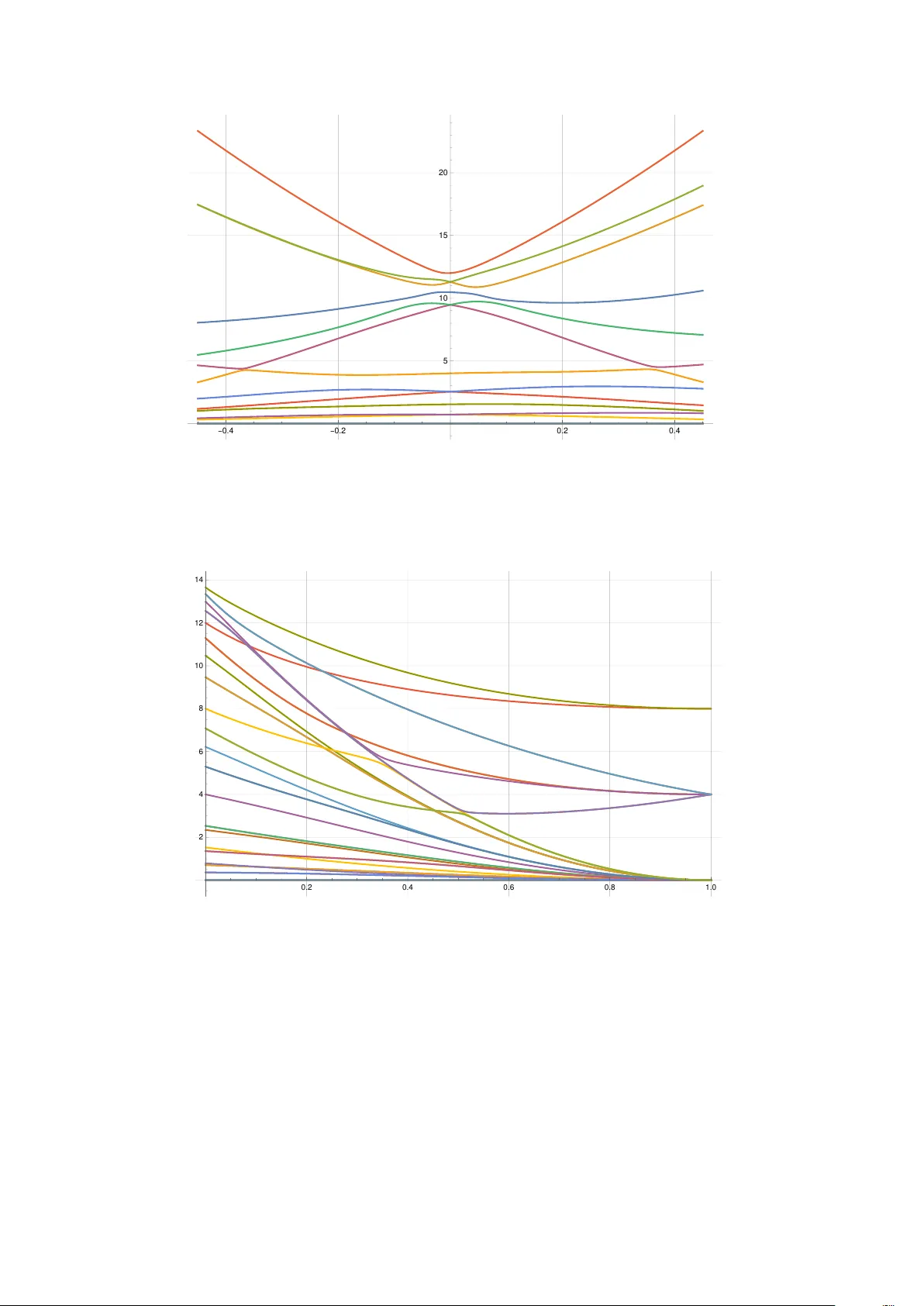
Spin c hains for ADE quiv er theories Jarryd Bath a and Konstan tinos Zoub os a,b a Departmen t of Ph ysics, Univ ersit y of Pretoria Priv ate Bag X20, Hatﬁeld 0028, South Africa and b National Institute for Theoretical and Computational Sciences (NITheCS) Gauteng, South Africa Abstract The sp ectral problem of four-dimensional superconformal quiver gauge theories can be mapp ed to one-dimensional spin c hains with restricted Hilb ert spaces, where the comp osition of neighbouring spins follows the path algebra of the quiver. T o b etter understand suc h spin c hains, w e compute the one-lo op planar dilatation op erator for the 4d N = 2 ADE quiv er gauge theories obtained by orbifolding the N = 4 Sup er-Y ang-Mills theory and marginally deforming b y indep enden tly v arying the gauge couplings. This extends previous work which was mainly fo cused on the Z 2 quiv er. W e characterise the general features of the resulting ADE spin-chain mo dels and construct the 2-magnon Bethe ansatz for holomorphic states. W e also ev aluate, at large N , the N = 2 sup erconformal index of these gauge theories and use it to study their protected sp ectrum in sp eciﬁc sectors. a jarryd.bath@tuks.co.za b kzoub os@up.ac.za Con ten ts 1 In tro duction 2 2 Orbifolding N = 4 SYM 4 2.1 Some ﬁnite group theory . . . . . . . . . . . . . . . . . . . . . . . . . . . . . . . . . . 4 2.2 The ﬁnite subgroups of SU(2) . . . . . . . . . . . . . . . . . . . . . . . . . . . . . . . 6 2.3 The orbifolding pro cedure . . . . . . . . . . . . . . . . . . . . . . . . . . . . . . . . . 8 2.4 The ADE Quiv er Lagrangian . . . . . . . . . . . . . . . . . . . . . . . . . . . . . . . 10 3 The planar ADE Dilatation Op erator 11 3.1 Reduction to N = 4 SYM diagrams . . . . . . . . . . . . . . . . . . . . . . . . . . . 12 3.2 Ev aluation of the F eynman diagrams . . . . . . . . . . . . . . . . . . . . . . . . . . . 14 3.3 Non-planar contributions at L = 2 . . . . . . . . . . . . . . . . . . . . . . . . . . . . 18 4 The ADE Hamiltonian 19 4.1 Holomorphic sector . . . . . . . . . . . . . . . . . . . . . . . . . . . . . . . . . . . . . 20 4.2 Mixed sector . . . . . . . . . . . . . . . . . . . . . . . . . . . . . . . . . . . . . . . . 20 5 The Protected Spectrum 21 5.1 N = 2 Represen tations and Shortening Conditions . . . . . . . . . . . . . . . . . . . 22 5.2 Review of the Sup erconformal Index . . . . . . . . . . . . . . . . . . . . . . . . . . . 24 5.3 Limits of the Index . . . . . . . . . . . . . . . . . . . . . . . . . . . . . . . . . . . . . 29 5.4 The ADE Index . . . . . . . . . . . . . . . . . . . . . . . . . . . . . . . . . . . . . . . 31 5.5 The Molien Series . . . . . . . . . . . . . . . . . . . . . . . . . . . . . . . . . . . . . 36 5.6 Example: The Z k theory . . . . . . . . . . . . . . . . . . . . . . . . . . . . . . . . . . 37 6 The ADE Spin chains 41 6.1 States of length 2 . . . . . . . . . . . . . . . . . . . . . . . . . . . . . . . . . . . . . . 42 6.2 Magnons on the ADE c hains . . . . . . . . . . . . . . . . . . . . . . . . . . . . . . . 44 7 Example: The Z 3 theory 45 7.1 The Z 3 Hamiltonian . . . . . . . . . . . . . . . . . . . . . . . . . . . . . . . . . . . . 46 7.2 Protected sp ectrum . . . . . . . . . . . . . . . . . . . . . . . . . . . . . . . . . . . . . 47 7.3 Short chains . . . . . . . . . . . . . . . . . . . . . . . . . . . . . . . . . . . . . . . . . 49 7.4 Tw o-magnon Bethe Ansatz . . . . . . . . . . . . . . . . . . . . . . . . . . . . . . . . 53 8 Example: The ˆ D 4 theory 58 8.1 The ˆ D 4 Hamiltonian . . . . . . . . . . . . . . . . . . . . . . . . . . . . . . . . . . . . 61 8.2 Protected sp ectrum . . . . . . . . . . . . . . . . . . . . . . . . . . . . . . . . . . . . . 63 8.3 Short chains . . . . . . . . . . . . . . . . . . . . . . . . . . . . . . . . . . . . . . . . . 65 8.4 Tw o-magnon Bethe Ansatz . . . . . . . . . . . . . . . . . . . . . . . . . . . . . . . . 71 9 Example: The ˆ E 6 theory 75 9.1 The ˆ E 6 Hamiltonian . . . . . . . . . . . . . . . . . . . . . . . . . . . . . . . . . . . . 77 9.2 Protected sp ectrum . . . . . . . . . . . . . . . . . . . . . . . . . . . . . . . . . . . . . 80 9.3 Short chains . . . . . . . . . . . . . . . . . . . . . . . . . . . . . . . . . . . . . . . . . 82 9.4 Tw o-magnon Bethe Ansatz . . . . . . . . . . . . . . . . . . . . . . . . . . . . . . . . 85 10 Discussion 89 A Character T ables of Finite Subgroups of SU(2) 92 1 B Adjacency matrices for the ﬁnite subgroups of SU(2) 93 C Sup erspace F eynman Rules 95 D Finiteness of the ADE theories 97 E Index of Some Short Multiplets 99 E.1 The ¯ E r (0 , 0) m ultiplet . . . . . . . . . . . . . . . . . . . . . . . . . . . . . . . . . . . . 100 E.2 The ˆ B R m ultiplet . . . . . . . . . . . . . . . . . . . . . . . . . . . . . . . . . . . . . . 101 E.3 Index of Some Op erators . . . . . . . . . . . . . . . . . . . . . . . . . . . . . . . . . . 101 F Extended SUSY T ransformations 103 G Konishi Descendants 105 G.1 Konishi descendan ts for Z 3 . . . . . . . . . . . . . . . . . . . . . . . . . . . . . . . . 106 G.2 Konishi descendan ts for ˆ D 4 . . . . . . . . . . . . . . . . . . . . . . . . . . . . . . . . 107 G.3 Konishi descendan ts for ˆ E 6 . . . . . . . . . . . . . . . . . . . . . . . . . . . . . . . . 108 1 In tro duction Quan tum ﬁeld theories with a large amoun t of supersymmetry are an ideal setting for obtaining exact results in Quantu m Field Theory . This is particularly true if they exhibit the prop ert y of planar integrabilit y , whic h allo ws for the computation of non-protected quan tities b oth as regards to the sp ectrum and correlation functions. The b est-understo od example is the N = 4 sup er-Y ang- Mills theory (SYM) where the planar dilatation operator w as shown to map, at one loop, to the Hamiltonian of a nearest-neigh b our Heisenberg spin chain [1]. The study of higher loops show ed that the spin chain remains integrable, with the Hamiltonian b ecoming increasingly long-range, whic h, together with insights from the dual AdS 5 × S 5 p erspective, led to the even tual solution of the N = 4 SYM sp ectral problem. W e refer to the reviews [2, 3, 4, 5] for details and references. It is imp ortan t to understand ho w m uch of the structure b ehind planar integrabilit y in N = 4 SYM is still present in theories with reduced sup ersymmetry . This question has b een studied extensiv ely for the N = 1 theories arising through marginal sup erp oten tial deformations of N = 4 SYM, as well as theories obtained via orbifolding (see e.g. [6] for a review). The orbifolding pro cess has b een shown to resp ect the integrable structures of N = 4 SYM [7, 8, 9, 10] including at higher-lo op [11, 12, 13]. How ev er, given an orbifold theory , one can marginally deform b y v arying the gauge couplings of eac h gauge group indep enden tly . The case of the marginally deformed Z 2 orbifold was ﬁrst studied in [14, 15, 16, 17]. Apart from its intrinsic interest, as explained in those w orks, an imp ortan t motiv ation for the study of this theory w as that, as one of the deformed couplings tends to zero, it limits to Sup erconformal QCD in the V eneziano limit [18]. Although N = 2 sup ersymmetry of course allo ws for the calculation of an abundance of protected quantities in the marginally deformed theories, the results of these early works were not encouraging with resp ect to integrabilit y . In particular, it quickly b ecame clear that standard structures such as the Y ang-Baxter equations w ere absen t and therefore the story of in tegrabilit y , if present, would necessarily b e more subtle. 1 Recen tly , the marginally deformed N = 2 orbifold theories were revisited with the goal of unco vering an y such additional structures and understanding what their implications would be. The w ork [23] studied the spin chains that arise in the holomorphic sector of the deformed Z 2 orbifold 1 These statemen ts refer to the scalar sector which w ould b e the analogue of the SO(6) sector in N = 4 SYM, on whic h we will fo cus in this w ork. The SU(2 , 1 | 2) sector of generic N = 2 SCFT, consisting of vector-m ultiplet ﬁelds, has b een argued to inherit the integrabilit y prop erties of N = 4 SYM, up to a redeﬁnition of the coupling constant [17, 19, 20, 21]. F or an early study of in tegrability for (non-conformal) pure N = 2 SYM, see [22]. 2 theory , and argued that the appropriate setting to understand them is that of dynamic al R -matrices, similar to those app earing in the study of elliptic quantum groups [24, 25]. Extending studies of the 2-magnon problem in [15, 23], the 3- and 4- magnon problems in a sp eciﬁc sector of these theories were considered in [26, 27] and sho wn to b e solv able b y taking long-range con tributions in to account. Meanwhi le, [28] to ok a step bac k and considered the underlying symmetries of the Z 2 theory , sho wing that the SU(4) generators which are brok en by the orbifolding pro cedure can b e usefully reco v ered b y w orking in a Lie algebroid, rather than a Lie algebra setting. The implications of these hidden symmetries and their p ossible relev ance to integrabilit y are still b eing w ork ed out. Giv en the progress made in the Z 2 theory , it is relev ant to explore the most general class of N = 2 theories that can b e obtained b y orbifolding N = 4 SYM and marginally deforming. These corresp ond to the ﬁnite subgroups of SU(2), which hav e an ADE classiﬁcation. As men tioned, it is kno wn that in tegrabilit y persists for suc h theories at the orbifold point [9, 10]. How ev er, b ey ond the case of Z 2 , the marginally deformed theories and their corresponding spin c hains ha ve not receiv ed m uch atten tion so far. In this w ork, we derive the one-lo op dilatation op erator for generic marginally-deformed ADE quiv er theories and discuss the main features of the corresp onding spin c hains. W e will b e partic- ularly in terested in the non-ab elian orbifold theories, whic h hav e some fundamental diﬀerences to the Z k cases. T o illustrate these diﬀerences, we treat some concrete examples, in particular the Z 3 , ˆ D 4 and ˆ E 6 cases, in more detail. F or the protected sp ectrum, we chec k our results b y comparing with sup erconformal index and Molien series computations. W e ﬁnd it us eful to p erform our deriv ation of the dilatation op erator fully in sup erspace. Since most suc h computations in the N = 4 SYM con text are p erformed in comp onents (for reviews, see e.g. [29, 30]), or fo cus only on the holomorphic sector [31, 32], w e pro vide some details of these computations. Apart from ensuring that our computations explicitly preserv e sup ersymmetry , w orking in sup erspace is lik ely to b e essential in extending our computations to higher lo ops, as w as done for the Z 2 quiv er in [33]. The outline of this paper is as follo ws: In Section 2 we review the pro cedure of orbifolding N = 4 SYM b y a subgroup of SU(2) to obtain the ADE quiv er theories. F or completeness, w e include some elemen ts from the theory of ﬁnite groups. In Section 3, w e discuss the sup erspace deriv ation of the ADE dilatation op erator, and summarise the corresp onding Hamiltonian in spin-c hain language in Section 4. In Section 5 we then switch gears to discuss the protected sp ectrum, and in particular ev aluate the sup erconformal index and its v arious limits for the ADE theories. In Section 6 w e summarise some generic features of the ADE spin chains. After this, we are ﬁnally ready to consider some concrete examples. W e study the Z 3 , ˆ D 4 and ˆ E 6 theories in Sections 7, 8 and 9, respectively . F or each example, we write out the Hamiltonian for that speciﬁc case, consider the protected states and, where possible, compare with the explicit diagonalisation, study the sp ectrum for short closed c hains, and ﬁnally construct the 2-magnon Bethe ansatz and compare the resulting energies and states with those found b y diagonalisation of the Hamiltonian. W e ha v e included several app endices with additional details on the ﬁnite subgroups of SU(2) (App endices A and B), our superspace conv en tions and F eynman rules (App endix C) (including, as a c heck, a veriﬁcation of the v anishing of the b eta function in Appendix D), more details on the index for some relev an t multiplets (App endix E), the on-shell N = 2 sup ersymmetry transformations (App endix F) and the explicit forms of the descendants of the Konishi op erator (Appendix G). 3 2 Orbifolding N = 4 SYM In this section w e will review the orbifolding pro cedure as applied to the N = 4 SYM theory . This sub ject has a long history , b eginning with [34, 35, 36, 37, 38, 39]. T aking a I IB string theory p erspective, recall the UV description of N = 4 SYM with gauge group SU( | Γ | N ) as a stack of | Γ | N D3-branes in 10-dimensional ﬂat space, with transv erse space | | | C 3 . Considering instead the orbifolded geometry | | | C 3 / Γ, with Γ a ﬁnite group of order | Γ | , one obtains | Γ | stacks of N D3 Branes, with Γ acting by p erm uting these stacks of branes. Orbifolding results in a certain collection of stac ks b eing identiﬁed as a single stac k and multiple stacks b eing identiﬁed with eac h other. The result is M stacks of n i N D3 branes each ( i = 1 , . . . , M ), with M b eing the num b er of conjugacy classes of Γ. F rom the ﬁeld theory p ersp ectiv e, one has constructed a gauge theory with Q M i =1 SU( n i N ) gauge group and ﬁelds in the adjoint or bifundamental represen tations of these groups, dep ending on the precise action of Γ. X 0 X 1 X 2 X 3 X 4 X 5 X 6 X 7 X 8 X 9 N D3 − − − − · · · · · · Γ-orbifold · · · · × × × × · · T able 1: Type I IB engineering of N = 2 orbifold daughters of N = 4 SYM. In practice, one can just work at the level of the ﬁeld theory , b y asking that the ﬁelds of SU( | Γ | N ) N = 4 SYM are inv ariant under the combined action of the ﬁnite group on the gauge as w ell as the R -symmetry indices. Φ I = R I J ( g ) γ reg ( g )Φ J γ − 1 reg ( g ) , g ∈ Γ . (2.1) Here g are the elements of the ﬁnite group and γ reg ( g ) is a sp eciﬁc representation of g on the SU( | Γ | N ) indices, to be elab orated b elo w. The matrix R I J ( g ) is the induced representation of g on the R -symmetry indices. If one is in terested in preserving N = 2 supersymmetry , Γ is required to b e a ﬁnite subgroup of SU(2). In the next section we will review these groups and their represen tations, in order to b e able to imp ose the ab o ve condition. 2.1 Some ﬁnite group theory In this section we will review some bac kground material on ﬁnite groups. F or a more detailed exp osition, w e refer to textb ooks suc h as [40, 41]. Recall that for a ﬁnite group the order denotes the n umber of elements. Let Γ b e a ﬁnite group of order | Γ | with M unitary irreducible representations (irreps) r i = ( ρ i , V i ), for i = 1 , . . . , M , where V i is a vector space and ρ i : Γ 7→ GL( V i ) is the action of the group on V i . F or a ﬁnite group M equals the n um b er of conjugacy classes. Let n i ≡ dim( r i ) and { ( e i ) 1 , . . . , ( e i ) n i } be a basis for the corresp onding v ector space V i . W e can then iden tify ρ i with its matrix elements: ρ i ( g ) m n ( e i ) m = ( e i ) n for g ∈ Γ . (2.2) The order of the group can b e expressed in terms of the representation space dimensions n i as | Γ | = M X i =1 n 2 i . (2.3) The unitary irreps satisfy the unitarity relation 1 | Γ | X g ∈ Γ ρ i ( g ) m n ¯ ρ j ( g ) k l = 1 n i δ ij δ m k δ l n . (2.4) 4 The pro duct representation of tw o irreps r k and r i can b e decomp osed as a sum ov er irreps: r k ⊗ r i = M M j =1 a k ij r j , (2.5) where a k ij denotes the m ultiplicity and is giv en b y a k ij = 1 | Γ | X g ∈ Γ χ k ( g ) χ i ( g ) ¯ χ j ( g ) , (2.6) where χ i ( g ) is the character of the element g in the represen tation r i . The equation (2.6) follows from the orthogonalit y relation for c haracters: X g ∈ Γ χ i ( g ) ¯ χ j ( g ) = | Γ | δ ij . (2.7) W e also hav e M X j =1 a k ij n j = n k n i . (2.8) F or simply reducible groups (whic h is the case for all the ﬁnite subgroups of SU(2) apart from Z 2 ), w e hav e either a k ij = 0 or a k ij = 1. The basis vectors of the pro duct representations and the irreps of simply reducible groups are related b y the Clebsch-Gordan co eﬃcien ts K j n kl , im as follows ( e k ) l ⊗ ( e i ) m = M X j =1 n j X n =1 K j n kl , im ( e j ) n . (2.9) F rom unitarity , we ha ve ( e j ) n = M X i,k =1 n i X m =1 n k X l =1 ¯ K j n kl , im ( e i ) m ⊗ ( e k ) l . (2.10) The Clebsch-Gordan co eﬃcien ts satisfy n i X m =1 n k X l =1 ¯ K j ′ n ′ kl , im K j n kl , im = δ j ′ j δ n ′ n and M X j =1 n j X n =1 ¯ K j n kl ′ , im ′ K j n kl , im = δ l ′ l δ m ′ m . (2.11) Let us now consider the inv arian t subspaces of pro duct representations. The Γ-in v arian t subspace of V i ⊗ V ∗ j is ( V i ⊗ V ∗ j ) Γ = { δ ij δ m n ( e i ) m ⊗ ( e ∗ j ) n } . (2.12) Hence from (2.9) and (2.12) we can ﬁnd the inv ariant subspace of V k ⊗ V i ⊗ V ∗ j : ( V k ⊗ V i ⊗ V ∗ j ) Γ = { ¯ K j n kl , im ( e k ) l ⊗ ( e i ) m ⊗ ( e ∗ j ) n } . (2.13) Let us consider an imp ortan t (reducible) representation: the regular represen tation r reg . The regular representation is the represen tation deﬁned b y dim( r reg ) = | Γ | . W e can interpret the regular represen tation as the represen tation acting on the ring o ver Γ, | | | C[Γ]. F ollowing [10], we refer to this as the “orbit basis” and denote it as r reg = ( τ , | | | C[Γ]). The matrix elements of τ can b e found as follo ws: τ ( g i ) m n = ( 1 , if g m g − 1 n = g i , 0 , otherwise . (2.14) 5 Essen tially , this means that the matrix elements of τ ( g i ) can b e found by setting 1 where the elemen t g i app ears in the Ca yley table of Γ. W e can also decomp ose the regular representation as a sum o ver ov er the irreps, which, again follo wing [10] we refer to as the “quiver basis”. W e will denote it as r reg = ( γ , V reg ). Let m i denote the multiplicit y of r i in r reg : r reg = M M i =1 m i r i . (2.15) The quiver basis takes the form of a blo ck diagonal matrix. Now notice that the order of the group is expressed in terms of the dimensions n i and the m ultiplicities as | Γ | = χ reg ( e ) = M X i =1 m i χ i ( e ) = M X i =1 m i n i , (2.16) where e is the iden tity elemen t of Γ. F rom (2.3), we ha ve m i = n i . Hence, we can write γ ( g i ) = M M i =1 ρ i ( g i ) ⊗ I n i × n i , V reg = M M i =1 V ⊕ n i i . (2.17) In the following sections, we will use the quiver basis matrices to imp ose inv ariance under the ﬁnite group action. 2.2 The ﬁnite subgroups of SU(2) In this section we review some well-kno wn asp ects of the ﬁnite subgroups of SU(2) [42]. They are the binary p olyhedral groups, sp eciﬁcally the binary cyclic, dihedral, tetrahedral, octahedral and icosahedral groups. Let us brieﬂy summarise their deﬁnition and structure. W e refer to App endix A for the character tables. 2.2.1 The cyclic group Z k The cyclic group Z k is deﬁned as { a | a k = e } . (2.18) where e is the iden tity element. It has order k and has k conjugacy classes, hence it also has k irreducible representations, which are all one-dimensional. Denoting b y ω k the k -th ro ot of unit y , these representations are simply the 1-dimensional matrices ρ n ( a ) = ω n k , (2.19) where n = 0 , . . . , k − 1 and where n = 0 is the trivial represen tation. 2.2.2 The binary dihedral group ˆ D k The binary dihedral group ˆ D k , also referred to as the dicyclic group Dic k (and also denoted by 2D k ) is a group of order 4 k − 8. It is given b y the following presen tation { a, b | a 2 n = e, b 2 = a n = z , b − 1 ab = a − 1 } , (2.20) where k = n + 2 and z is the cen tral element of order 2. F or k ≥ 4, the centre of the group is the tw o-element subgroup ⟨ z ⟩ , and the quotien t ˆ D k / ⟨ z ⟩ is the standard dihedral group D k of order 2 k − 4. ˆ D k has k + 1 conjugacy classes: { e } , { a n } , { a m , a − m } , { b, a 2 b, . . . , a 2 n − 2 b } , { ab, a 3 b, . . . , a 2 n − 1 b } . (2.21) 6 where m = 1 , . . . , n − 1. Corresp ondingly , there are k + 1 irreducible representations. Since the c haracters are simply the traces of the representations, the one-dimensional represen tations can b e read oﬀ from the c haracter tables in T ables 20 and 21. Elements in the same conjugacy class hav e the same 1-dimensional representations, but diﬀer in the 2-dimensional ones. The tw o-dimensional irreps are parametrised b y the o dd integers n = 1 , . . . , k − 1: ρ ( a ) =  ω m 2 n 0 0 ω − m 2 n  and ρ ( b ) =  0 − 1 1 0  . (2.22) 2.2.3 The binary tetrahedral group 2T This is a non-ab elian group of order 24, deﬁned as { r , s, t | r 2 = s 3 = t 3 = r st = z } , (2.23) where z is the central element of order 2. Equiv alently , we can write r = z t − 1 s − 1 , hence, r 2 = ( t − 1 s − 1 z ) 2 = ( st ) − 2 = z . Now since z − 1 = z , w e hav e that z = ( st ) 2 . Thus, we can write the binary tetrahedral group as { s, t | ( st ) 2 = s 3 = t 3 = z } . (2.24) In terms of quaternions, the generators can b e written as r = ˆ i, s = 1 2 (1 + ˆ i + ˆ j − ˆ k ) , t = 1 2 (1 + ˆ i + ˆ j + ˆ k ) . (2.25) 2T has sev en conjugacy classes and hence sev en irreducible represen tations. They are presen ted in Section 9. 2.2.4 The binary o ctahedral group 2O This is a non-ab elian group of order 48, with the following presentation { r , s, t | r 2 = s 3 = t 4 = r st } , (2.26) equiv alently { s, t | ( st ) 2 = s 3 = t 4 } . (2.27) It has 8 conjugacy classes/irreducible representations. W e refer to e.g. [43] for its representations. 2.2.5 The binary icosahedral group 2I This is an non-ab elian subgroup of order 120, with the following presentation { r , s, t | r 2 = s 3 = t 5 = r st } , (2.28) equiv alently { s, t | ( st ) 2 = s 3 = t 5 } . (2.29) It has 8 conjugacy classes/irreducible representations. W e again refer to e.g. [43] for more details. Through the McKa y corresp ondence [44], these groups are related to the aﬃne ˆ A k , ˆ D k , ˆ E 6 , ˆ E 7 and ˆ E 8 Lie groups, resp ectiv ely . Concretely , the Dynkin diagrams of these aﬃne groups, sho wn in Fig. 1, provide the adjacency diagrams of the binary p olyhedral groups. The adjacency matrices for all ADE cases are listed in App endix B. W e note that Z 2 is the only non-simply laced case, indicated b y a double line in the Dynkin diagram and corresp ondingly a 2 in the adjacency matrix. This leads to a degeneracy in the orbifolding pro cedure which requires the use of an additional lab el. As the Z 2 orbifold theory and its deformations is well studied [14, 15, 23, 28], in the following we will fo cus on the case of Z k with k > 2, and will therefore not include this additional degeneracy lab el in our notation. 7 ˆ A 1 : 1 1 ˆ A k : 1 1 1 1 1 ˆ D k : 1 1 2 2 2 2 1 1 ˆ E 6 : 1 2 3 2 1 2 1 ˆ E 7 : 1 2 3 4 3 2 1 2 ˆ E 8 : 2 4 6 5 4 3 2 1 3 Figure 1: The Dynkin Diagrams for the aﬃne ˆ A, ˆ D and ˆ E series. Each no de has an asso ciated Kac index n i , which denotes the corresp onding vector space dimension. When orbifolding by the corresp onding subgroup of SU(2), these Dynkin diagrams b ecome the quiver diagrams of the orbifolded theories, with each no de asso ciated to a SU( n i N ) gauge group. 2.3 The orbifolding pro cedure Orbifolding by a ﬁnite subgroup of SU(2) breaks the SU(4) R R -symmetry group of N = 4 SYM to SU(2) L / Γ × SU(2) R × U(1) r . The action of the un broken R-symmetry group on the ﬁelds is summarised in T able 2. Given a ﬁnite subgroup of SU(2), orbifolding requires us to imp ose φ ab σ + R σ − R σ 3 R σ r X 0 ¯ Y 1 2 X 0 Y 0 − ¯ X 1 2 Y 0 Z 0 0 0 − Z ¯ X − Y 0 − 1 2 ¯ X 0 ¯ Y X 0 − 1 2 ¯ Y 0 ¯ Z 0 0 0 ¯ Z T able 2: The action of su (2) R × u (1) r on the ﬁelds of N = 4 SYM. in v ariance of the ﬁelds under Γ. As mentioned, Γ also acts on the R -symmetry index of the ﬁelds. Ho wev er, in our N = 2 case we ha ve the decomp osition 3 = 2 ind ⊕ 1 triv , where 2 ind is the induced represen tation that arises from Γ b eing a subgroup of SU(2) and 1 triv is the trivial representation. The action can therefore b e written as R = R ( 2 ) ⊕ 1 . (2.30) Therefore Γ acts on the vector ﬁeld of N = 4 SYM, as well as on one of the chiral m ultiplets (whic h w e call Φ 3 = Z ) simply b y conjugation, and in v ariance implies: V = γ reg ( g ) V γ − 1 reg ( g ) , Z = γ reg ( g ) Z γ − 1 reg ( g ) , g ∈ Γ . (2.31) 8 The other tw o chiral ﬁelds of N = 4 SYM, Φ 1 = X and Φ 2 = Y , transform under the SU(2), so they are also acted up on b y the induced represen tation: Φ I = R I J ( g ) γ reg ( g )Φ J γ − 1 reg ( g ) , g ∈ Γ . (2.32) The ﬁelds of the mother theory decomp ose as [ V ] im j n = δ i j δ m n V i , [Φ I ] im j n = K im 3 I , j n Q ij , for I = 1 , 2 , [Φ 3 ] im j n = δ i j δ m n Z i , [ ¯ Φ I ] im j n = ¯ K j n 3 I , im ¯ Q ij , for I = 1 , 2 , [ ¯ Φ 3 ] im j n = δ i j δ m n ¯ Z i . (2.33) As is well kno wn, this pro cedure leads to U( N ) groups, with the U(1) factors ha ving non-trivial β functions and thus sp oiling the conformal inv ariance. As discussed in [45, 46], in tegrating out these U(1) factors leads to SU( N ) gauge groups and restores conformalit y , but also results in the addition of quartic double-trace terms in the component Lagrangian of the theory , arising b y integrating out the U(1) parts of the adjoint F Z and D auxiliary ﬁelds. W e are therefore left with a quiver gauge theory with pro duct gauge group Y i SU( n i N ) . (2.34) The matter con tent is expressed in terms of the adjacency matrix a 3 ij = 1 | Γ | X g ∈ Γ χ 3 ( g ) χ i ( g ) ¯ χ j ( g ) , (2.35) where a nonzero elemen t with i = j denotes an adjoin t ﬁeld while a nonzero element with i  = j a bifundamen tal. These matrices are tabulated in App endix B. F or N = 2 theories, all gauge groups ha ve a corresp onding adjoin t ﬁeld, forming an N = 2 v ector m ultiplet. Therefore a 3 ii = 1 for any i . So to fo cus on the bifundamental ﬁelds b et ween no des i and j , we can subtract the diagonal part of the adjacency matrix: a 2 ij ≡ a 3 ij − δ ij . (2.36) Giv en the non-c hiral nature of the N = 2 theory , if the m ultiplet Q ij is in the □ × ¯ □ representation of the SU( N i ) × SU( N j ) gauge groups, the Q j i m ultiplet will b e in the conjugate ¯ □ × □ represen tation. The i th N = 1 v ector m ultiplet V i com bines with the i th adjoin t m ultiplet Z i to form an N = 2 v ector m ultiplet, while the t wo N = 1 c hiral multiplets Q ij and Q j i com bine to form an N = 2 h yp erm ultiplet. Let us denote by M the num b er of gauge groups/no des of the quiver, and by H the num b er of hypermultiplets. T able 2.3 summarises these num b ers for the ADE groups. Quiv er ˆ A k ˆ D k ˆ E 6 ˆ E 7 ˆ E 8 Γ Z k +1 ˆ D k 2T 2O 2I | Γ | k + 1 4 k − 8 24 48 120 M k + 1 k + 1 7 8 9 H k + 1 k 6 7 8 T able 3: The orbifold group, the corresp onding ˆ A ˆ D ˆ E classiﬁcation, n umber of no des and num b er of hypermultiplets for the N = 2 orbifolds. 9 This information can b e conv enien tly expressed in a quiv er diagram, which is based on the corresp onding aﬃne Dynkin diagram (see Fig. 1), with each no de corresp onding to a SU( n i N ) gauge group and with the num b er of lines b et ween no des determined b y the a 3 ij matrix. Gauge theories with these pro duct gauge groups, called ADE quiv er theories, were ﬁrst studied in [47] with a focus on their Higgs-branch geometry , which was understoo d in a mirror-symmetry con text in [48]. In the follo wing it will be con v enient to deﬁne the weigh ted (by the size of the gauge group) adjacency matrix d ij ≡ 2 X I ,J =1 n i ,n j X m,n =1 ε I J 3 K j n 3 I , im K im 3 J, j n . (2.37) As this matrix will app ear in the sup erp oten tial, w e call it the sup erp oten tial co eﬃcient matrix. It satisﬁes d j i = − d ij , (2.38) and ¯ d ij d ij = n 2 i n 2 j . (2.39) F rom (2.39), we hav e | d ij | 2 = n 2 i n 2 j , hence (taking d ij to b e real) w e ha ve d ij = ± a 2 ij n i n j . (2.40) The choice of sign in (2.40) is conv en tional 2 . In the concrete cases that we will study , we will b e writing Q ij → X ij / Y ij , in suc h a wa y that Q ij → X ij if d ij = − 1 and Q ij → Y ij if d ij = +1. The quiv ers clearly ha v e discrete symmetries related to relab elling the no des (p erm uting the branes in the s tring theory construction). F or a complete list of the outer automorphisms of the ADE quiv ers, w e refer to [49]. The symmetry group of the Z k quiv ers is also Z k , and is implemented b y the τ ( g ) matrices deﬁned ab o v e acting b y conjugation. These matrices (or at least a suitable subset of them) are exp ected to play a similar role in the non-ab elian quiv ers, as we will see in our examples. As we will come back to in Section 6, the orbifold theories allow for twiste d se ctors , which can b e obtained by inserting the γ ( g ) matrix in the gauge trace of single-trace op erators. O g = T r  γ ( g )Φ I 1 Φ I 2 . . . Φ I L − 1 Φ I L  . (2.41) Therefore, the sp ectrum of the theory at the orbifold p oin t will organise itself in separate t wisted sectors. W e will indicate the states b elonging to each sector in our sp eciﬁc examples. 2.4 The ADE Quiv er Lagrangian Ha ving describ ed the ﬁeld conten t of the general N = 2 ADE quiver theory in the previous section, w e are ready to write do wn the N = 1 sup erspace Lagrangian that one obtains by the orbifolding pro cedure. As the Z 2 case has b een extensively treated in previous w orks (e.g. [14, 15]) we will fo cus on the simply reducible case where there are no multiplicities in the pro ducts of irreducible represen tations. W e will also let the couplings of eac h gauge no de v ary indep endently: g i YM = κ i g YM . (2.42) The Lagrangian one obtains is given b y S N =2 , Γ = S vector + S ghost + S chiral , where: 2 The ambiguit y in the sign of d ij follo ws from the fact that the Clebsch-Gordan co eﬃcien ts K j n 3 I , im are unique up to a c hoice in phase. 10 S vector = M X i =1 n i g 2 YM κ 2 i Z d 4 x T r i  1 4  Z d 2 θ ( W α ) i ( W α ) i + h.c.  − 1 ξ i Z d 4 θ D 2 V i ¯ D 2 V i  , S ghost = M X i =1 n i Z d 4 xd 4 θ T r i   c ′ i + ¯ c ′ i  L g YM κ i 2 V i  c i + ¯ c i + coth L g YM κ i 2 V i ( c i − ¯ c i )  , S chiral = M X i =1 n i Z d 4 xd 4 θ T r i  e − g YM κ i V i ¯ Z i e g YM κ i V i Z i  + M X i,j =1 a 2 ij n i n j Z d 4 xd 4 θ T r j  e − g YM κ j V j ¯ Q j i e g YM κ i V i Q ij  +  Z d 4 xd 2 θ W Γ + h.c.  (2.43) where ( W α ) i ≡ i ¯ D 2  e − g YM κ i V i D α e g YM κ i V i  , (2.44) and the sup erpotential is given b y W Γ = ig YM M X i,j =1 g YM κ i d j i T r j ( Q j i Z i Q j i ) . (2.45) W e ha v e highligh ted in red the diﬀerences to the N = 2 theory due to the orbifolding pro cedure, and in blue the marginal deformation parameters κ i whic h tak e the theory aw a y from the orbifold p oin t. The superspace F eynman rules arising from the ab o ve Lagrangian are summarised in App endix C. As is well kno wn [36, 37], the orbifolded theories inherit the ﬁniteness prop erties of N = 4 SYM. As also discussed in those works, c hanging the gauge couplings a w ay from their orbifold-p oint v alues as in (2.42) is a marginal deformation preserving N = 2 sup erconformal in v ariance. Although this can b e argued in general, it is also straightforw ard to directly chec k that the v anishing of the b eta functions is unaﬀected by the deformation. F or completeness, we sho w this in App endix D. As w e will ev entually w an t to study the spectrum of these theories in terms of comp onen t ﬁelds, it is crucial to know ho w the ﬁelds are related by sup ersymmetry transformations. Therefore, we list the unbrok en on-shell N = 2 sup erc harges and sho w their actions on the comp onen t ﬁelds in App endix F. 3 The planar ADE Dilatation Op erator In this section we provide some details of the computation of the one-loop dilatation operator of the ADE quiv er theories, in the full scalar sector. In N = 4 SYM, this computation was p erformed in [1], leading to the SO(6) XXX Hamiltonian. F or reviews and additional details, see [29, 30]. W e will work in an N = 1 sup ersymmetric setting. See [32, 31] for previous sup erspace approaches to the N = 4 dilatation op erator and [33] for the N = 2 Z 2 orbifold case. Similar techniques w ere also emplo yed in [50] in the study of a sp eciﬁc N = 1 marginal deformation of N = 4 SYM. In the ab o v e works, the fo cus w as on higher-lo op computations where the use of sup erspace was essen tial. Ho wev er, ev en in our one-lo op case w e ﬁnd that sup erspace simpliﬁes some of the computations and of course guaran tees that our result is fully sup ersymmetric. F urthermore, working in comp onents often entails ﬁxing the sup ersymmetric gauge to b e the W ess-Zumino gauge, in order to reduce the n umber of auxiliary ﬁelds. Ho wev er, the W ess-Zumino gauge explicitly breaks sup ersymmetry , with the result that the fundamen tal ﬁelds of the theory acquire non-zero anomalous dimensions, 11 naiv ely making the theory app ear to b e non-ﬁnite. Of course, as we verify in App endix D, w orking in sup erspace the ﬁniteness of the theory is eviden t, as the anomalous dimensions of all fundamental ﬁelds v anish. F or a recent review of sup erspace tec hniques as applied to N = 2 sup ersymmetric gauge theory , see [51]. The sup erspace notation and F eynman rules that we use largely follow [52] and are summarised in App endix C. W e are interested in computing the one-lo op, planar contribution to the t wo p oin t function ⟨ O ∆ ( x ) ¯ O ∆ ( y ) ⟩ = 1 ( x − y ) 2∆ , (3.1) where O ∆ ( x ) are gauge-inv ariant op erators in the quiver gauge theory . W e fo cus on the scalar sector, where the op erators are made up of the lo w est comp onen ts of the sup erﬁelds Q ij , ¯ Q ij , Z i , ¯ Z i . Due to the planar limit, the one-lo op con tributions are a sum of interactions b et ween neighbouring ﬁelds, which allows us to reduce the problem to ﬁnding all (divergen t) one-lo op contributions to all p ossible pairs of ﬁelds. Rather than ev aluating the t w o-p oin t function directly , W e will tak e an eﬀectiv e v ertex approach [53, 54] where one do es not consider the ¯ O ( y ) op erator but only the outgoing ﬁelds from the one- lo op corrected O ( x ) op erator. Renormalising each operator as O I ren = Z I J ( λ, ϵ ) O J bare , the action of the dilatation op erator will b e given by D I J = 2Res ϵ =0  λ d dλ log Z I J ( λ, ϵ )  . (3.2) where the ’t Ho oft coupling is deﬁned as λ = g 2 YM N . As this action mixes diﬀeren t monomials in the ﬁelds, constructing the op erators with deﬁnite scaling dimensions ∆ amounts to diagonalising the dilatation op erator. 3.1 Reduction to N = 4 SYM diagrams Giv en the structure of the ADE Lagrangian (2.43), it is clear that all the F eynman diagrams will b e the same as in N = 4 SYM, but no w decorated with diﬀerent c hoices of gauge groups as w ell as a dep endence on the κ i co eﬃcien ts of the marginally deformed theory . In this section, we will therefore ﬁrst k eep trac k of these diﬀerences to N = 4 SYM. The F eynman in tegrals themselv es will b e the same as in N = 4 SYM, and will b e ev aluated in the next subsection. As a ﬁrst example of how the ADE theory diagrams map to those of N = 4 SYM, consider the follo wing diagram giving the correction to · · · Q ij Q j i · · · . W e read the diagram from the bottom up, and the dotted line indicates that in computing the eﬀectiv e vertex we only consider the diagram up to this p oin t, and in particular the top index lo op is not counted. Q ij Q j i ¯ Q ik ¯ Q ki = κ 2 i ¯ d j i d ki n j n 3 i × X Y ¯ X ¯ Y ¯ Z Z (3.3) The colouring of the double lines in the N = 2 diagram represen ts the diﬀeren t no des under which the corresp onding ﬁeld is charged. The conv en tion is that diﬀerent colours on the same propagator 12 are exclusive, so in the ab ov e c ase i  = j and i  = k , but it could b e that k = j . The planar diagram on the right represents the N = 4 SYM case, where there is only one no de and therefore only one type of gauge group index. The notation is sligh tly sc hematic in that in the N = 2 diagram, the choice of X vs. Y ﬁelds is determined by the sp eciﬁc choice made for Q ij for a given quiver, so it actually corresp onds to four N = 4 SYM diagrams. These diagrams hav e diﬀerent signs (sc hematically , X Y → X Y vs. X Y → − Y X ) which in the N = 2 case are taken care of by the d ij co eﬃcien ts. Note that the p o w ers of n i come b oth from the index lo ops as well as the propagators as listed in App endix C. Suppressing the dotted line in the following, w e can similarly relate Q ij Z j ¯ Q ij ¯ Z j = κ 2 j ¯ d ij d ij = κ 2 j X Z ¯ X ¯ Z ¯ Y Y (3.4) and Q ij Z j ¯ Z i ¯ Q ij = κ i κ j ¯ d ij d j i = − κ i κ j X Z ¯ X ¯ Z = κ i κ j ¯ Y Y X Z ¯ Z ¯ X ¯ Y Y (3.5) The transposed diagrams with Z Q at the b ottom are equal to the ab o ve. As we will discuss in the next section, diagrams with gauge b oson exchange in the holomorphic sector are ﬁnite b y p ow er coun ting. So the ab ov e are all the diagrams in the holomorphic sector whic h are UV div ergent and con tribute to the dilatation op erator. The diagrams for the antiholomorphic sector are the conjugates of the ab o ve and will take equal v alues. So w e no w need to consider the diagrams in the mixed sector, i.e. where one ﬁeld is holomorphic and the other antiholomorphic. T o sav e space, w e will only indicate the factors that diﬀer from the corresp onding N = 4 SYM diagrams, which are straightforw ard to repro duce. Let us ﬁrst write the diagrams with v ertical gauge ﬁelds, whic h are Q ij ¯ Q j i Q ik ¯ Q ki = 1 2 κ 2 i n k n i = − Q ij ¯ Q j i ¯ Q ik Q ki , Q ij ¯ Q j i Z i ¯ Z i = 1 2 κ 2 i n i = − Q ij ¯ Q j i ¯ Z i Z i . , (3.6) 13 as well as Z i ¯ Z i Z i ¯ Z i = 1 2 κ 2 i = − Z i ¯ Z i ¯ Z i Z i , Z i ¯ Z i Q ij ¯ Q j i = 1 2 κ 2 i n j = − Z i ¯ Z i ¯ Q ij Q j i . . (3.7) Then we ha ve iden tity-t yp e diagrams with horizon tal gauge ﬁeld exc hange: Q ij ¯ Q j k ¯ Q ij Q j k = − κ 2 j , Z i ¯ Z i ¯ Z i Z i = − κ 2 i , Q ij ¯ Z j ¯ Q ij Z j = − κ 2 j . (3.8) Finally , we ha ve diagrams with horizontal chiral ﬁeld exchange, Q ij ¯ Q j k Q ij ¯ Q j k = κ 2 j ¯ d ij d kj n i n k n 2 j , Q ij ¯ Q j i Z i ¯ Z i = κ 2 i ¯ d j i d j i n i = κ 2 i n i , (3.9) as well as Z i ¯ Z i Q ij ¯ Q j i = κ 2 i ¯ d j i d j i n j = κ 2 i n j , Q ij ¯ Z j Z i ¯ Q ij = κ i κ j ¯ d j i d ij = − κ i κ j . (3.10) In the next section we will see that all the ab ov e F eynman diagrams are prop ortional to a single one-lo op in tegral. 3.2 Ev aluation of the F eynman diagrams Ha ving expressed all the con tributions to the planar dilatation op erator in terms of their N = 4 SYM counterparts, the next step is to ev aluate the corresp onding integrals. As w e ha v e already tak en the gauge index structure into account, in this section w e will drop the double-line notation. 14 Let us use the follo wing shorthand notation for a 1-lo op F eynman integral: I ( λ, µ, ϵ ) ≡ λµ 2 ϵ = λµ 2 ϵ Z d 4 − 2 ϵ k (2 π ) 4 − 2 ϵ 1 k 2 ( k 2 − p 2 ) . (3.11) As we will see, all the 1-lo op diagrams contributing to the dilatation op erator will turn out to b e prop ortional to this in tegral. A standard computation gives I ( λ, µ, ϵ ) = λ Γ( ϵ )Γ(1 − ϵ ) 2 16 π 2 Γ(2 − 2 ϵ )  4 π µ 2 p 2  ϵ = λ 16 π 2  1 ϵ − γ E + log  4 π µ 2 p 2  + O ( ϵ )  , (3.12) where Γ( ϵ ) is the standard Gamma function and γ E is the Euler-Masc heroni constan t. Then 2Res ϵ =0  λ d dλ I ( λ, µ, ϵ )  = 2 λ 16 π 2 . (3.13) T o ev aluate the diagrams of the previous section, let us quickly revise some sup ergraph rules (for more details, see [52, 55], as well as the review [31]): Each vertex introduces an integral ov er the fermionic co ordinates d 4 θ while eac h lo op introduces an in tegral ov er the unconstrained lo op momen tum d 4 − 2 ϵ p . W e can slide cov ariant deriv atives D α (or ¯ D ˙ α ) across propagators, pic king up a minus sign each time: D α = − D α (3.14) Note that w e m ust k eep the ordering of the D’s the same as w e slide them ¯ D ˙ α D α = ¯ D ˙ α D α  = D α ¯ D ˙ α (3.15) In tegration b y parts on the sup ergraph is depicted as D α = D α + D α (3.16) W e also ha v e to take into account that every time w e p erform an integration by parts on a b osonic function, we get a min us sign, and every time we p erform an integration by parts on a fermionic function, we get a plus sign. Note that when we p erform the integration by parts, we alwa ys in tegrate so that the cov ariant deriv ative furthest aw a y from the v ertex is mov ed ﬁrst: D β D α = D α D β + D α D β = D α D β + D α D β + D α D β + D α D β (3.17) W e also recall that D 3 = ¯ D 3 = 0, so we can only hav e a maximum of tw o D’s and t wo ¯ D’s sequen tially on a line. F urthermore we use the iden tities D α D α = − D 2 , ¯ D ˙ α ¯ D ˙ α = − ¯ D 2 , (3.18) and also that D 2 ¯ D 2 D 2 = □ D 2 and ¯ D 2 D 2 ¯ D 2 = □ ¯ D 2 . (3.19) 15 In momentum space, a factor of □ purely introduces a factor of − p 2 , where p is the momentum of the propagator that □ is attached to. Finally , we hav e Z d 4 θ ¯ D 2 D 2 δ (4) ( θ ) = Z d 4 θ D 2 ¯ D 2 δ (4) ( θ ) = 1 . (3.20) W e mak e use of (3.20) to collapse integrals ov er momentum space and of the fermionic co ordinates o ver pro ducts of delta functions in fermionic co ordinates to integrals o ver only momentum space: if we ha ve a lo op where a single propagator has either ¯ D 2 D 2 or D 2 ¯ D 2 attac hed to it, and all other propagators in that lo op hav e no co v arian t deriv ativ es attac hed to it, then that integral is localised in sup erspace and is conv erted to a regular in tegral o ver momen tum space. As in e.g. [32, 31, 33], w e will indicate this lo calisation to a regular momen tum space lo op by shading in the lo op. W e ﬁrst consider the c hiral diagrams. Recall that we are treating the comp osite op erators as a v ertex inserted at a p oin t. F rom sup erspace rules, due to how functional deriv ativ es with resp ect to c hiral ﬁelds are deﬁned, eac h chiral ﬁeld in a diagram alw ays in tro duces a factor of D 2 . How ev er, in order to con vert the superspace in tegral o ver a chiral vertex from one b eing ov er half of sup erspace d 2 θ , we conv ert one of the sup erspace deriv ativ es ¯ D 2 in to the measure d 2 ¯ θ to get a total measure of d 4 θ . This means that whenever we hav e a chiral vertex consisting of m ﬁelds, w e alwa ys ha ve m − 1 cov ariant deriv atives ¯ D 2 at that v ertex. Since w e treat the op erator insertions as a vertex, if the comp osite op erator is c hiral and comprised of L ﬁelds, we will alwa ys hav e L − 1 cov arian t deriv atives ¯ D 2 at this insertion. Let us also recall that the sup erﬁcial degree of div ergence of a sup ergraph is given b y [52] D ∞ = 2 − C − E c , (3.21) where C is the n umber of ΦΦ or ¯ Φ ¯ Φ propagators (whic h are only relev ant for massive theories) and E c is the n umber of external chiral or an ti-chiral lines. In considering the sup erﬁcial degree of div ergence, we will b e cutting the diagram ab o v e the lo op and will b e treating the op erator as an external line. So we can immediately conclude that ¯ D 2 ¯ D 2 ¯ D 2 D 2 D 2 → D ∞ = − 1 → ﬁnite (3.22) i.e. when both ﬁelds are holomorphic, the gauge b oson exc hange diagrams are ﬁnite and do not con tribute. F or the holomorphic sector, w e therefore only consider the chiral diagrams (3.3),(3.4) and (3.5). T o ev aluate the corresp onding N = 4 SYM diagrams, w e apply the D-algebra until w e obtain a lo op containing a single D 2 and a single ¯ D 2 . As explained, the lo op integral is then con verted in to a regular lo op: ¯ D 2 D 2 D 2 ¯ D 2 ¯ D 2 = D 2 ¯ D 2 ¯ D 2 ¯ D 2 → − I ( λ, µ, ϵ ) (3.23) In the ﬁnal step we conv erted the d 4 θ integral at the top vertex into d 2 θ ¯ D 2 to fully localise the fermionic co ordinates and then the remaining D 2 and ¯ D 2 com bine as a □ , cancelling the propaga- tor betw een the c hiral and anti-c hiral v ertex and w e are left with an o verall factor of − 1 as the propagator of the chiral ﬁeld is of the form − □ − 1 . 16 Let us now mov e on to the mixed sector. Since the comp osite op erators comprise b oth c hiral and anti-c hiral ﬁelds, the comp osite op erator cannot b e chiral and w e can no longer apply the logic of removing one co v ariant deriv ative ¯ D 2 as we argued ab ov e in the case of c hiral comp osite op erators. The ev aluation of the diagrams of type (3.6) and (3.7) go es as ¯ D 2 D 2 D 2 ¯ D 2 = D 2 ¯ D 2 D 2 ¯ D 2 = D 2 ¯ D 2 D 2 ¯ D 2 = ¯ D 2 D 2 D 2 ¯ D 2 = ¯ D 2 D 2 D 2 ¯ D 2 = D 2 ¯ D 2 → I ( λ, µ, ϵ ) (3.24) Note that the factor D 2 ¯ D 2 again contributes a □ to the diagram and fully lo calises the fermionic co ordinates, how ever, now the vector sup erﬁeld’s propagator is of the form □ − 1 , thus the relative sign diﬀerence b etw een (3.23) and (3.24). F or the mixed diagrams with gluon exc hange (3.8) we ﬁnd ¯ D 2 D 2 D 2 ¯ D 2 D 2 ¯ D 2 ¯ D 2 D 2 = ¯ D 2 D 2 D 2 ¯ D 2 D 2 ¯ D 2 ¯ D 2 D 2 = ¯ D 2 D 2 D 2 ¯ D 2 ¯ D 2 D 2 ¯ D 2 D 2 = ¯ D 2 D 2 D 2 ¯ D 2 ¯ D 2 □ D 2 = ¯ D 2 D 2 D 2 ¯ D 2 □ ¯ D 2 D 2 = ¯ D 2 D 2 D 2 ¯ D 2 D 2 ¯ D 2 □ = ¯ D 2 D 2 D 2 ¯ D 2 D 2 ¯ D 2 □ = ¯ D 2 D 2 D 2 ¯ D 2 D 2 ¯ D 2 □ = ¯ D 2 D 2 D 2 ¯ D 2 D 2 ¯ D 2 □ = D 2 ¯ D 2 D 2 ¯ D 2 □ → I ( λ, µ, ϵ ) (3.25) Lastly , for the mixed diagrams with exc hange of an N = 1 chiral m ultiplet (3.9) and (3.10), the D-algebra gives 17 ¯ D 2 D 2 ¯ D 2 D 2 D 2 ¯ D 2 D 2 ¯ D 2 = ¯ D 2 ¯ D 2 D 2 D 2 ¯ D 2 D 2 D 2 ¯ D 2 = ¯ D 2 ¯ D 2 D 2 D 2 ¯ D 2 D 2 D 2 ¯ D 2 = ¯ D 2 ¯ D 2 D 2 □ D 2 D 2 ¯ D 2 = ¯ D 2 D 2 □ D 2 ¯ D 2 D 2 ¯ D 2 = ¯ D 2 D 2 □ ¯ D 2 D 2 D 2 ¯ D 2 = ¯ D 2 D 2 □ ¯ D 2 D 2 D 2 ¯ D 2 = ¯ D 2 D 2 □ ¯ D 2 D 2 D 2 ¯ D 2 = ¯ D 2 D 2 □ D 2 ¯ D 2 D 2 ¯ D 2 = ¯ D 2 ¯ D 2 D 2 □ D 2 D 2 ¯ D 2 = ¯ D 2 ¯ D 2 D 2 □ D 2 ¯ D 2 D 2 = ¯ D 2 D 2 ¯ D 2 D 2 □ → − I ( λ, µ, ϵ ) (3.26) Ha ving expressed all the required F eynman diagrams in terms of I ( λ, µ, ϵ ), we can now extract the div ergent parts using (3.13). They will b e simply ± 1 times the standard λ/ (16 π 2 ) prefactor. So, up to this factor, the one-lo op dilatation op erator is simply equal to the group-theoretic co eﬃcien ts of the diagrams in Section 3.1. W e will write out the resulting Hamiltonian in Section 4. Before that, how ever, w e need to consider a sp ecial class of non-planar contributions whic h need to b e considered for op erators of length 2. 3.3 Non-planar con tributions at L = 2 As w e are working in the strict planar limit, in the ab o ve computations w e hav e ignored non-planar eﬀects. In particular, we hav e treated the propagators of the adjoint ﬁelds as if they were in U( N ) rather than SU( N ). The diﬀerence is subleading in all cases, apart from the case of length-2 op erators, where the diagrams sho wn in Fig. 2 are b oth of order N 4 . Therefore, these eﬀects need to be taken into account. In the comp onen t formalism, these con tributions lead to double-trace terms in the Lagrangian (see e.g. [15] for the Z 2 orbifold case), arising from in tegrating out the D - terms and the adjoint F Z - terms. As w e are w orking in sup erspace, w e don’t ha ve double-trace terms but w e can compute these con tributions directly . Their eﬀect is to precisely cancel the planar part of the dilatation op erator for certain op erators, bringing their eigen v alues from their planar v alues down to E = 0. It is easy to see that these non-planar diagrams only con tribute to twisted sectors, as the tw o cyclic orderings of the three-p oin t v ertex giv e opp osite signs, but result in the same trace operators. Clearly , this non-planar correction aﬀects a whole SU(2) R triplet at once:   Q ij Q j i 1 √ 2 ( Q ij ¯ Q j i − ¯ Q ij Q j i ) ¯ Q ij ¯ Q j i   . (3.27) Therefore, these non-planar con tributions lead to the protection of the twisted-sector L = 2 SU(2) R triplets, on top of the un twisted triplet (whic h is also present for the cyclic quiv ers). As explained 18 Q ij Q j i − 1 N Q ij Q j i , Q ij ¯ Q j i − 1 N Q ij ¯ Q j i Figure 2: F or L = 2, the 1 / N part of the adjoint propagators gives a leading contribution in the large N limit. There are t wo more diagrams, for ¯ QQ and ¯ Q ¯ Q . in [15], these sp eciﬁc triplets are guaranteed to b e protected by index argumen ts, and, as w e will see, the same is true in our ADE case. So this non-planar eﬀect is crucial in obtaining agreement with index computations. 4 The ADE Hamiltonian Ha ving computed all the one-lo op diagrams that contribute to the planar dilatation op erator, in this section we will presen t the resulting one-lo op Hamiltonian for generic ﬁnite subgroups of SU(2). Recall that, in ev aluating the diagrams, w e restricted to the lo w est scalar components of the sup erﬁelds, so the Hamiltonian b elo w will b e for the scalar comp onen ts of the X , Y , Z sup erﬁelds (and their conjugates). Since no more sup erﬁelds will app ear in the remainder of this article, will not sp eciﬁcally indicate this and use X , Y , Z to indicate the scalar comp onen ts from now on. 3 As already discussed, the Hamiltonian for orbifolds of N = 4 SYM is integrable at the orbifold p oin t, where all the gauge couplings are equal [7, 8, 9, 10]. So our main interest will b e in the marginally deformed theories, which we will call ADE quiver spin chains. F or the Z 2 quiv er, the marginally deformed theory was treated in detail in [14, 15]. It w as called the interp olating the ory , since it in terp olates from the orbifold p oint g (1) YM = g (2) YM to sup erconformal QCD (in the V eneziano limit) when one of the gauge couplings is tak en all the wa y to zero. Among the ADE quiv ers, the Z 2 theory is special in that it has an additional SU(2) L symmetry , under which the X and Y bifundamen tal ﬁelds form a doublet. So in this case the full un broken symmetry group is SU(2) L × SU(2) R × U(1) r . The un broken SU(2) L pla yed an important role in the study of the X Y sector in [23], where the spin chain is an alternating Heisenberg mo del. Here our main fo cus will b e on all the other quiver theories, whic h do not ha ve this symmetry enhancemen t. The Hamiltonian H is read oﬀ from the one lo op dilatation op erator as D (1) = − λ 16 π 2 H . (4.1) A t one lo op, the Hamiltonian is nearest-neighbour, so we can express its action on eac h pair of sites on the spin c hain: H = L X ℓ =1 H ℓ,ℓ +1 , (4.2) where for closed chains w e hav e L + 1 ≃ 1. W e will exhibit the one-lo op scalar Hamiltonian through its action on the diﬀerent sectors of the theory . Clearly , the Hamiltonian will dep end on 3 It would b e straightforw ard to include the fermions of the chiral multiplets, as it would simply inv olve additional co v ariant deriv ativ es in the F eynman diagrams. How ever, a full treatment b ey ond the scalar sector would require the inclusion of gauge ﬁeld and gaugino insertions, which we leav e for future work. 19 the adjacency matrix of a giv en quiver as well as the ranks of the v arious gauge groups. These are summarised in the co eﬃcien ts d ij deﬁned in (2.40). It is also conv enien t to deﬁne the quantit y H i ≡ P M j =1 a 2 ij , which is simply the num b er of hypermultiplets attac hed to a no de. 4.1 Holomorphic sector It is easy to see that H ℓ,ℓ +1 = 0 on Z i Z i , (4.3) and, for i  = k : H ℓ,ℓ +1 = 0 on Q ij Q j k . (4.4) The Hamiltonian on bifundamentals whic h return to the same no de is H ℓ,ℓ +1 = 2 κ 2 i n 3 i          ¯ d ij 1 d ij 1 n j 1 ¯ d ij 1 d ij 2 n j 1 . . . ¯ d ij 1 d ij H i n j 1 ¯ d ij 2 d ij 1 n j 2 ¯ d ij 2 d ij 2 n j 2 . . . ¯ d ij 2 d ij H i n j 2 . . . . . . . . . . . . ¯ d ij H i d ij 1 n j H i ¯ d ij m i d ij 2 n j H i . . . ¯ d ij H i d ij H i n j H i          in the basis      Q ij 1 Q j 1 i Q ij 2 Q j 2 i . . . Q ij H i Q j H i i      (4.5) while on one bifundamental and one adjoin t w e ha ve H ℓ,ℓ +1 =  2 κ 2 i − 2 κ i κ j − 2 κ i κ j 2 κ 2 j  in the basis  Z i Q ij Q ij Z j  . (4.6) The action of the Hamiltonian on an tiholomorphic ﬁelds can b e found by conjugation. 4.2 Mixed sector Here we need to distinguish t wo cases, when the Hamiltonian acts on t wo sites with the same ﬁrst and last index, or when the indices are diﬀerent. F or the ﬁrst case, let us deﬁne the column vectors: Q ¯ Q i ≡    Q ij 1 ¯ Q j 1 i . . . Q ij H i ¯ Q j H i i    , ¯ QQ i ≡    ¯ Q ij 1 Q j 1 i . . . ¯ Q ij H i Q j H i i    . (4.7) W e also deﬁne the H i × H i matrices M i ≡ κ 2 i n i    n j 1 . . . n j H i . . . . . . . . . n j 1 . . . n j H i    , T i ≡    2 κ 2 j 1 . . . 2 κ 2 j H i    , (4.8) and the H i × 1 and 1 × H i matrices L i ≡     κ 2 i n i . . . κ 2 i n i     , K i ≡  κ 2 i n j 1 . . . κ 2 i n j H i  . (4.9) Using these, w e can express the mixed Hamiltonian in compact form as H ℓ,ℓ +1 =     3 κ 2 i − κ 2 i K i K i − κ 2 i 3 κ 2 i K i K i L i L i T i + M i T i − M i L i L i T i − M i T i + M i     in the basis     Z i ¯ Z i ¯ Z i Z i Q ¯ Q i ¯ QQ i     . (4.10) 20 W e note that, written in this w a y , the Hamiltonian is not hermitian since L is not equal to K † . This is due to the non-canonical normalisations used in the Lagrangian (2.43), and can be easily ﬁxed b y rescaling the ﬁelds b y appropriate factors of √ n i . This w ould, how ev er, introduce suc h square-ro ot factors in the Hamiltonian. Therefore, and since this do es not aﬀect the sp ectrum (whic h is of course real) w e ﬁnd it b est to keep the non-canonical normalisation. F or the case when k  = i , w e ha ve H ℓ,ℓ +1 =    2 κ 2 j 2 κ 2 j d kj ¯ d ij n i n k n 2 j 2 κ 2 j ¯ d kj d ij n i n k n 2 j 2 κ 2 j    in the basis  Q ij ¯ Q j k ¯ Q ij Q j k  . (4.11) and ﬁnally H ℓ,ℓ +1 =     2 κ 2 i − 2 κ i κ j − 2 κ i κ j 2 κ 2 j 2 κ 2 i − 2 κ i κ j − 2 κ i κ j 2 κ 2 j     in the basis     Z i ¯ Q ij ¯ Q ij Z j ¯ Z i Q ij Q ij ¯ Z j     . (4.12) where w e note that the Hamiltonian do es not mix the ﬁrst t wo with the second t wo rows, as that w ould violate the U(1) r symmetry . One can straigh tforw ardly chec k that the ADE Hamiltonian comm utes with the SU(2) R × U(1) r R-symmetry group, whose action is shown in T able 2. Of course, unlik e the Z 2 Hamiltonian computed in [15], it do es not comm ute with the SU(2) L symmetry under whic h the X and Y ﬁelds w ould form a doublet. W e emphasise that the abov e Hamiltonian is only v alid for L > 2, as it do es not accoun t for the non-planar contributions at L = 2 discussed in section 3.3. F or L = 2, the states aﬀected by those contributions (which, as discussed, are t wisted sector states in the triplet represen tation of SU(2) R ) will still appear as eigenstates of the Hamiltonian but with non-zero energy , instead of the correct E = 0. As these states are easily identiﬁable, in the following we will use the Hamiltonian also for L = 2 and set the eigen v alues of these sp eciﬁc states to zero b y hand. Before pro ceeding to discuss the spin c hains on whic h this Hamiltonian acts, we need to dev elop a second to ol in the study of the ADE theories, namely the sup erconformal index and its v arious limits. This will pro vide crucial information on the protected sp ectrum of our theories. R eaders who are more interested in non-protected quan tities can jump ahead to Section 6. 5 The Protected Sp ectrum In the previous sections, we computed the one-lo op scalar dilatation op erator of the ADE theories and expressed it as a spin-c hain Hamiltonian. This pro vides a wealth of information ab out the sp ectrum of the theory , although it is of course limited to scalar op erators and will receive higher- lo op corrections. As in N = 4 SYM, the scalar sector will also not b e closed at higher lo ops. Also, ev en though (as w e will sho w) it is possible to solv e the 2-magnon problem for the ADE spin c hains, and th us obtain all-length results, the higher-magnon problem is expected to b e signiﬁcan tly more complicated. F or these reasons, follo wing in the fo otsteps of [14, 15] for the Z 2 orbifold theory , we will also consider another p ow erful tool to aid us in the study of the ADE theories, namely the sup erconformal index [56, 57]. T ogether with the Molien series (whic h has already b een applied to the ADE quivers in [43]), it will provide additional, coupling-indep endent information on the sp ectrum of protected states. Besides allowing us to access fermionic parts of the sp ectrum, it will pro vide additional chec ks of the Hamiltonian b y considering the o verlap of the t wo approac hes. In the follo wing sections, w e will brieﬂy review the multiplets of N = 2 sup ersymmetry and the deﬁnition of the sup erconformal index, b efore ev aluating it for the ADE quiver theories. 21 5.1 N = 2 Represen tations and Shortening Conditions In this section, w e will brieﬂy introduce some of the N = 2 representations whic h will play a role in the computation of the index, as well as in the study of the sp ectrum by direct diagonalisation of our Hamiltonian. F or more details and pro ofs, w e refer to [58, 59, 60, 61], as w ell as the p edagogical treatmen ts in [51, 62]. Our notation will mainly follo w [60]. In this notation | R , r ⟩ h.w. satisﬁes the follo wing under SU(2) R ⊗ U(1) r (see T able 2): σ + R | R, r ⟩ h.w. = 0 , σ 3 R | R, r ⟩ h.w. = R | R, r ⟩ h.w. , σ r | R, r ⟩ h.w. = r | R, r ⟩ h.w. . (5.1) Let us now review some of the represen tation theory of the N = 2 sup erconformal algebra. W e will b egin by giving the necessary commutation and anti-comm utation relations. F or the full sup erconformal algebra, see e.g. [51, 62]. Recall that the algebra includes the b osonic generators P µ , M β α , ¯ M ˙ β ˙ α , K µ , D , R i j , r (where R i j = σ ± , 3 R ) and fermionic generators Q i α , ¯ Q i ˙ α , S β j , ¯ S j ˙ β , where i = 1 , 2 and α, ˙ α are the spacetime SU(2) × SU(2) indices. As is standard, we will b e writing α = ± , ˙ α = ˙ ± . First, we hav e the following commutation relations [ D , Q i α ] = + 1 2 Q i α , [ D , ¯ Q i ˙ α ] = + 1 2 ¯ Q i ˙ α , [ D , S α i ] = − 1 2 S α i , [ D , ¯ S i ˙ α ] = − 1 2 ¯ S i ˙ α , (5.2) whic h imply that the sp ecial conformal sup erc harges, S α i and ¯ S i ˙ α , lo wer the scaling dimension ∆ b y 1 2 and the Poincar ´ e sup erc harges, Q i α and ¯ Q i ˙ α , raise the scaling dimension ∆ by 1 2 4 . Next, we ha ve the following an ti-commutation relations {Q i α , S β j } = 1 2 δ i j δ β α D + δ i j M β α − δ β α R i j − 1 2 δ i j δ β α r , { ¯ Q i ˙ α , ¯ S j ˙ β } = 1 2 δ j i δ ˙ β ˙ α D + δ j i ¯ M ˙ β ˙ α + δ ˙ β ˙ α R j i − 1 2 δ j i δ β α r . (5.3) Consider a state in the Hilb ert space H on R × S 3 for a N = 2 SCFT. W e let | ∆ , j 1 , j 2 ; R , r ⟩ ∈ H , where ∆ is the scaling dimension (the eigen v alue of the dilatation op erator D ), R is the Dynkin lab el of su (2) R , r is the u (1) r c harge, and ( j 1 , j 2 ) are the Dynkin lab els of the Lorentz algebra su (2) 1 × su (2) 2 . As men tioned, the S sup erc harges low er the scaling dimension by 1 2 . Because w e w ant to consider representations with a bounded sp ectrum of D , we require that there exist states | ∆ , j 1 , j 2 ; R , r ⟩ ∈ H satisfying K µ | ∆ , j 1 , j 2 ; R , r ⟩ = 0 , S α i | ∆ , j 1 , j 2 ; R , r ⟩ = 0 , ¯ S i ˙ α | ∆ , j 1 , j 2 ; R , r ⟩ = 0 . (5.4) These states are called sup er c onformal primaries (whic h we refer to as primaries for brevity). The represen tations of H are then spanned b y the descendants of the sup erconformal primaries, obtained b y acting with the Poincar ´ e sup ercharges: Y i,j,α, ˙ α ( ¯ Q i ˙ α ) n i ˙ α ( Q j α ) n j α | ∆ , j 1 , j 2 ; R , r ⟩ , n i ˙ α , n j α = 0 , 1 . (5.5) A sup erconformal primary (5.4) and its descendants (5.5) form a m ultiplet. The Hilb ert space H is spanned b y the primaries and their descendan ts. W e consider unitary theories, where all states hav e non-negativ e norms, || | ∆ , j 1 , j 2 ; R , r ⟩|| ≥ 0. Conjugation acts as ( Q i α ) † ≡ S α i , ( ¯ Q i ˙ α ) † ≡ ¯ S i ˙ α , (5.6) 4 Often in the literature ¯ Q and ¯ S are denoted e Q and e S . The tilde notation is used b ecause, while in Lorentzian signature ¯ Q = Q † and ¯ S = S † , in Euclidean signature the left and right-handed spinors are indep enden t. 22 so that ⟨Q i α Ψ   = ⟨ Ψ | S α i , ⟨ ¯ Q i ˙ α Ψ   = ⟨ Ψ | ¯ S i ˙ α . (5.7) Let us no w consider the norms of the ﬁrst descendants of a superconformal primary | ∆ , j 1 , j 2 ; R , r ⟩ . Computing the norms of Q i ± and ¯ Q i ˙ ± on this state, applying (5.3), and requiring p ositivit y gives ( 1 2 ∆ ± j 1 + ( − 1) i R − 1 2 r ) || | ∆ , j 1 , j 2 ; R , r ⟩|| 2 ≥ 0 , ( 1 2 ∆ ± j 2 + ( − 1) i R + 1 2 r ) || | ∆ , j 1 , j 2 ; R , r ⟩|| 2 ≥ 0 . (5.8) F rom unitarity , we ha ve || | ∆ , j 1 , j 2 ; R , r ⟩|| 2 ≥ 0, hence, from (5.8), we must ha ve 5 ∆ ≥ max { 2 + 2 j 1 + 2 R + r , 2 + 2 j 2 + 2 R − r } ≡ f ( j 1 , j 2 , R , r ) . (5.9) In (5.9) we are excluding the trivial represen tation of SU(2 , 2 | 2) (the v acuum state), with ∆ = 0 [62, 51]. The constraint on ∆ in (5.9) is called a unitary b ound . The unitary b ounds (5.9) in SCFTs pla y an analogous role to the p ositive semi-deﬁnite energy condition in SUSY QM. Zero norm states (or nul l states ) decouple from the theory; hence, we only need to consider primaries with p ositiv e deﬁnite norms || | ∆ , j 1 , j 2 ; R , r ⟩|| > 0 and remo v e those with zero norms. If a primary state | ∆ , j 1 , j 2 ; R , r ⟩ saturates the unitary bound, then one of its descendan ts will be n ull and hence will decouple from the theory , i.e. one of the states will be annihilated b y the action of one (or more) P oincar´ e sup ercharges, Q i α or ¯ Q i ˙ α . Therefore, the multiplet generated from this primary will con tain fewer states than a m ultiplet generated by a primary whose dimension is strictly greater than the unitary b ound (5.9). Hence, we call the multiplets that saturate the unitary b ound (5.9) short multiplets and the m ultiplets strictly ab o ve the unitary b ound (5.9) long multiplets . F or reference, we provide a list of these N = 2 SCFT multiplets in T able 4, follo wing the classiﬁcation sc heme of [60]. Multiplet Op erator ( R, ℓ ≥ 0 , n ≥ 2) ˆ B 1 T r h P M ( 3 ) ij i ˆ B R +1 T r  P ( Q ij Q j i ) R +1  ¯ E − ( ℓ +2)(0 , 0) T r h P Z ℓ +2 i i ˆ C R (0 , 0) T r  P T ( Q ij Q j i ) R  ¯ D R +1(0 , 0) T r h P 1 m =0 ( Q ij Q j i ) R +1 Z m i Z 1 − m j i D R + 3 2 (0 , 1 2 ) T r h P 1 m =0 ( Q ij Q j i ) R +1 ( ¯ λ i ) m Z ˙ + ( ¯ λ j ) 1 − m Z ˙ + i ¯ B R +1 , − ( ℓ +2)(0 , 0) T r h P ℓ +2 m =0 ( Q ij Q j i ) R +1 Z m i Z ℓ +2 − m j i ¯ C R, − ( ℓ +1)(0 , 0) T r h P ℓ +1 m =0 T ( Q ij Q j i ) R Z m i Z ℓ +1 − m j i C R, ( ℓ +1)(0 , 0) T r h P ℓ +1 m =0 T ( Q ij Q j i ) R ¯ Z m i ¯ Z ℓ +1 − m j i A 2 R + ℓ +2 n R, − ℓ (0 , 0) T r h P ℓ m =0 T n ( Q ij Q j i ) R Z m i Z ℓ − m j i T able 4: The sup erconformal primaries of some of the m ultiplets of the N = 2 superconformal alge- bra, adapted from [14]. In the sc hematic notation used there, the symbol P indicates summation o ver all symmetric traceless p ermutations of the comp onen t ﬁelds as allow ed b y the gauge index structure, and T stands for an R -symmetry-neutral combination of scalar ﬁelds. Note that R can b e half-in teger. A generic long multiplet is denoted by A 2 R + ℓ +2 n R,r ( j 1 ,j 2 ) . F or the shortening conditions of eac h multiplet 5 There are some short multiplets with stricter unitary b ounds suc h that f ( j 1 , j 2 , R, r ) ≥ ∆ ≥ 1 [51, 62] 23 in T able 4, w e refer to [14]. In N = 2 theories, ¯ E r (0 , 0) corresp onds to Coulomb branc h physics and ˆ B R corresp onds to Higgs branc h ph ysics. In the quan tum theory , short multiplets can only acquire anomalous dimensions ∆ = f ( j 1 , j 2 , R , r ) + γ ( λ ) , (5.10) (where λ is a coupling) if they recom bine with other short multiplets and b ecome long. That is, the descendan ts that w ere lost due to the existence of a null vector are returned. The rules that dictate how m ultiplets can recombine are called r e c ombination rules and are listed in [60]. 5.2 Review of the Sup erconformal Index In studying the sp ectrum of N = 2 theories, it would b e of great in terest to consider a protected ob ject counting precisely the short m ultiplets that do not b ecome long. This ob ject, known as the sup erconformal index, was in tro duced in [56, 57], see [63, 64] for reviews. In our discussion b elo w, w e will closely follo w the treatment in [65] 6 . Let us deﬁne the following ob jects δ i ± ≡ 2 {Q i ± , S ± i } , ¯ δ i ˙ ± ≡ 2 { ¯ Q i ˙ ± , ¯ S i ˙ ± } . (5.11) F rom (5.6), w e hav e that δ i ± ≥ 0 and ¯ δ i ˙ ± ≥ 0. W e can write δ i ± and ¯ δ i ˙ ± in terms of the quantum n umbers of the states: δ i ± = ∆ ± 2 j 1 + ( − 1) i 2 R − r , ¯ δ i ˙ ± = ∆ ± 2 j 2 + ( − 1) i 2 R + r , (5.12) This leads to the general sup erconformal index in tro duced in [56, 57], deﬁned as follows: I ( µ i ) = T r H ( − 1) F e − µ i T i e − β δ , (5.13) where the trace is o v er the Hilb ert space H of the theory deﬁned on S 1 β × S 3 . β is the circum- ference of the thermal circle S 1 β and { T i } a complete set of generators that comm ute with the sup erc harge Q in δ that we “deﬁne the index with resp ect to” and with each other, and { µ i } are the corresp onding chemical p oten tials. The sup erconformal index (5.13) counts the states with δ = 0, hence, Q | ∆ , j 1 , j 2 ; R , r ⟩ = 0, and is therefore β -indep enden t. By the state-op erator cor- resp ondence, counting (with grading) states on R × S 3 is equiv alen t to coun ting (with grading) lo cal op erators on R 4 . The states with δ = 0 are called BPS states , and form short m ultiplets of the sup erconformal algebra. The sup erconformal index is a generalisation of the Witten index [66] for sup ersymmetric quantum mechanics to the sup erconformal ﬁeld theory context. Like the Witten index, it is inv ariant under marginal deformations of the theory and hence is insensitive to marginal changes of couplings. So it is a protected quan tity , and a computation of the index in the free theory will still b e v alid in the quan tum theory . F or four-dimensional N = 2 SCFTs, whic h are non-c hiral, diﬀerent choices of Q result in ph ysically equiv alen t indices. The subalgebra of su (2 , 2 | 2) comm uting with a single sup erc harge is su (1 , 1 | 2), whic h has rank three, so the N = 2 index depends on three sup erconformal fugacities [65]. 7 W e choose to deﬁne our index with resp ect to ¯ Q 1 ˙ − . A basis of the Cartan generators of the comm utant subalgebra su (1 , 1 | 2) is giv en b y δ 1 − , δ 1+ , ¯ δ 2 ˙ + . (5.14) 6 Ho wev er, note that to match the notation in App endix F, we use a diﬀeren t conv en tion for the lab els for the N = 2 vector-m ultiplet fermions. 7 Theories with ﬂav our symmetries ha ve additional fugacities, ho wev er we will not b e considering such theories in this w ork. 24 With this c hoice of generators, (5.13) b ecomes I ( ρ, σ, τ ) = tr H ( − 1) F ρ 1 2 δ 1 − σ 1 2 δ 1+ τ 1 2 ¯ δ 2 ˙ + e − β ¯ δ 1 ˙ − , (5.15) where the trace runs ov er the states of the theory on S 3 , and for con vergence we take | ρ | < 1 , | σ | < 1 , | τ | < 1. The charges of the states coun ted b y this index ob ey the shortening condition ¯ δ 1 ˙ − = ∆ − 2 j 2 − 2 R + r = 0 . (5.16) As discussed in [65], another common parametrisation of the index is in terms of fugacities ( p, q , t ), related to ( σ, ρ, τ ) as p = τ σ , q = τ ρ, t = τ 2 . (5.17) In terms of these fugacities the index (5.15), reads I ( p, q , t ) = tr H ( − 1) F p j 2 + j 1 − r q j 2 − j 1 − r t R + r e − β ¯ δ 1 ˙ − . (5.18) where conv ergence requires | p | < 1 , | q | < 1 , | t | < 1 ,   pq t   < 1 . W e will mostly present our results in this second parametrisation. In the follo wing, we will ev aluate the superconformal index (5.13) for general ADE orbifold quiv er theories in the N → ∞ limit 8 . The Z k index was calculated in [67]; how ever, in dividing out the U(1) factors, only the con tributions from the N = 1 v ector multiplet were considered rather than the N = 2 vector m ultiplet, leading to an N = 1 index. T aking this into accoun t, the N = 2 index for the Z 2 quiv er was computed in [14]. This theory has an additional SU(2) L symmetry compared to the generic ADE case, and therefore has an additional fugacit y . T o our knowledge, the large- N sup erconformal index of non-ab elian orbifolds has not b een directly computed in the literature. W e will pro vide its general form for an y N = 2 orbifold theory and then ev aluate it in the sp eciﬁc examples that we are cov ering. F ollowing the plethystic programme [43], w e b egin b y writing down the generalisation of a single-letter index with the single letters given b y the fundamental ﬁelds and deriv ativ es. W e list the single-letter con tributions to the index in T able 5. Letters ∆ j 1 j 2 R r I ( σ, ρ, τ ) I ( p, q , t ) Z 1 0 0 0 − 1 σ ρ pq t − 1 ¯ λ Z ˙ + 3 2 0 1 2 1 2 1 2 − τ 2 − t λ V ± 3 2 ± 1 2 0 1 2 − 1 2 − σ τ , − ρτ − p, − q ¯ F ˙ + ˙ + 2 0 1 0 0 σ ρτ 2 pq ∂ − ˙ + λ V + + ∂ + ˙ + λ V − = 0 5 2 1 2 0 1 2 − 1 2 σ ρτ 2 pq Q ij 1 0 0 1 2 0 τ t 1 2 ¯ ψ j i ˙ + 3 2 0 1 2 0 1 2 − σ ρτ − pq t − 1 2 ∂ ± ˙ + 1 ± 1 2 1 2 0 0 σ τ , ρτ p, q T able 5: Letters in the N = 2 v ector multiplet and half-hypermultiplet with ¯ δ 1 ˙ − = 0. The other half of the hypermultiplet has contributing letters ( Q j i , ¯ ψ ij ˙ + ) which hav e the same charges as ( Q ij , ¯ ψ j i ˙ + ) but transform in a conjugate represen tation of the gauge and global symmetry . In addition to the ( ρ, σ, τ ) / ( p, q , t ) fugacities, we need to introduce a fugacity with resp ect to the 8 Note that, in the N → ∞ limit, the sup erconformal index counts the Kaluza-Klein states in the gravit y dual theory [57]. 25 gauge symmetries, as the sp ectrum of the theory is given by gauge in v arian t operators. The v ector m ultiplet at no de i con tributes i vm ( U i ; ρ, σ, τ ) =  − σ τ 1 − σ τ − ρτ 1 − ρτ + σ ρ − τ 2 (1 − σ τ ) (1 − ρτ )  χ adj ,i ( U i ) =  1 + pq t − 1 + pq − t − 1 (1 − p )(1 − q )  χ adj i ( U i ) , (5.19) where χ adj i ( U i ) is the c haracter of the adjoint represen tation of the i th gauge group. A h yp erm ul- tiplet connecting no des i and j contributes i hm ( U i , U j ; ρ, σ, τ ) = τ (1 − ρσ ) (1 − ρτ )(1 − στ )  χ □ i × □ j ( U i , U j ) + χ □ i × □ j ( U i , U j )  = t 1 2 (1 − pq t − 1 ) (1 − p )(1 − q )  χ □ i × □ j ( U i , U j ) + χ □ i × □ j ( U i , U j )  , (5.20) where □ i × □ j denotes the bifundamental representation and □ i × □ j its conjugate. W e will use the following notation for the characters of the adjoin t and bifundamental representations: χ ii ( U ii ) ≡ χ adj , i ( U i ) = T r i U i T r i U † i − 1 , (5.21a) χ ij ( U ij ) ≡ χ □ i × □ j ( U i , U j ) = T r i U i T r j U † j , (5.21b) where the U i ’s are in the fundamen tal represen tation. F or Γ  = Z 2 , there is no ﬂav our group generically . How ev er, through deformations of the couplings, a gauge group can b ecome global and turn in to a ﬂav our group, which is not a marginal deformation (as it changes the structure of the Hilb ert space). Hence, the following computations will apply to generic couplings where no gauge groups b ecome global. F rom T able 5, one ﬁnds that the single-letter index asso ciated to no de i is i ( U ; p, q , t ) = M X i,j =1 χ ij ( U ij ) ( δ ij f vm ( p, q , t ) + f hm ( p, q , t )) . (5.22) where we ha ve deﬁned f vm ( p, q , t ) ≡ 1 − (1 − pq t − 1 )(1 + t ) (1 − p )(1 − q ) = 1 − (1 − ρσ )(1 + τ 2 ) (1 − τ σ )(1 − τ ρ ) , f hm ( p, q , t ) ≡ t 1 2 (1 − pq t − 1 ) (1 − p )(1 − q ) = τ (1 − ρσ ) (1 − ρτ )(1 − στ ) . (5.23) F or our sp eciﬁc ADE quivers, it is useful to deﬁne the quan tity f ij ( p, q , t ) ≡ δ ij f vm ( p, q , t ) + a 2 ij f hm ( p, q , t ) , (5.24) Then, we can write the single-letter index (5.22) as i ( U ; p, q , t ) = M X i,j =1 χ ij ( U ij ) f ij ( p, q , t ) . (5.25) Notice that this index coun ts the adjoint ﬁelds at each no de, but, to av oid o ver-coun ting, only one half-h yp erm ultiplet from each arrow linking the no de to other nodes. The other half-hypermultiplets will b e counted together with the other no des. 26 No w that we hav e the single-letter index (5.25), w e apply the plethystic programme [68] to compute the index. Let us ﬁrst deﬁne the pleth ystic exp onen tial (PE) PE[ f ( x i )] := exp ∞ X n =1 f ( x n i ) n ! . (5.26) Then, the full index can b e found via the plethystic exponential of the single letter index [64] I ( U ; p, q , t ) = PE[ i ( U ; p, q , t )] . (5.27) Ho wev er, (5.27) counts all op erators, not just gauge inv ariant op erators (which are the ph ysical states in the spectrum). In order to pro ject out the gauge in v arian t op erators, w e will need to mak e use of Sc hur’s orthogonalit y relation for Lie group c haracters, whic h states that Z U ∈ G [ dU ] χ R ( U ) χ R ′ ( U ) = δ RR ′ , (5.28) where [ dU ] is the Haar measure of G . W e can rewrite the in tegral o ver the matrices in (5.28) as an in tegral o ver the fugacities (the eigenv alues of U ) as Z U ∈ G [ dU ] f ( U ) = N Y m =1 I | u m | =1 du m 2 π iu m ∆( u ) f ( u ) , (5.29) where N is the rank of the group and ∆( u ) is the V andermonde determinan t, whic h ev aluates to ∆( u ) = PE " X α u α #! − 1 = PE " − X α u α # = Y α (1 − u α ) , (5.30) where P α u α ≡ P α Q m u α i m , where α i are the ro ots of the Lie algebra. Notice that χ adj ( u ) = P α u α so that ∆( u ) = PE[ − χ adj ( u )] . (5.31) W e can now write the pro jection of the index on the trivial representation as I | trivial = N Y m =1 I | u m | =1 du m 2 π iu m PE[ i ( x ; u m ) − χ adj ( u )] χ trivial ( u ) , (5.32) in other w ords, to obtain the gauge-inv ariant op erators, w e just need to integrate o ver the u i . Let us introduce some useful functions that will help us express the indices in a compact form. First of all, the q -P o c hhammer sym b ol ( z ; q ) ∞ is deﬁned b y ( z ; q ) ∞ ≡ ∞ Y i =0 (1 − z q i ) = exp − ∞ X n =1 1 n z n (1 − q n ) ! , (5.33) The elliptic Γ function Γ( t ; p, q ) is deﬁned by [69] Γ( t ; p, q ) ≡ ∞ Y i,j =0 (1 − t − 1 p i +1 q j +1 ) (1 − tp i q j ) = exp ∞ X n =1 1 n t n − p n q n t − n (1 − p n )(1 − q n ) ! . (5.34) It satisﬁes the following iden tities that will b e useful to us later [69]: Γ( pq t − 1 ; p, q ) = 1 Γ( t ; p, q ) , Γ( q ; p, q ) = ( p ; p ) ∞ ( q ; q ) ∞ , Γ( t ; 0 , q ) = ( t ; q ) − 1 ∞ and Γ( t ; 0 , 0) = 1 1 − t . (5.35) 27 F rom (5.33) and (5.34), we immediately ﬁnd the follo wing useful expression PE[ f vm ( p, q , t )] = exp ∞ X n =1 f vm ( p n , q n , t n ) n ! = exp ∞ X n =1 1 n  − p n 1 − p n − q n 1 − q n + p n q n t − n − t n (1 − p n )(1 − q n )  ! = ( p ; p ) ∞ ( q ; q ) ∞ Γ( t ; p, q ) . (5.36) F rom (5.34), we obtain the expression PE[( v + v − 1 ) f hm ( p, q , t )] = exp ∞ X n =1 ( v n + v − n ) f hm ( p n , q n , t n ) n ! = exp ∞ X n =1 v n t n 2 − p n q n v − n t − n 2 + v − n t n 2 − p n q n v n t − n 2 (1 − p n )(1 − q n ) ! =Γ( v t 1 2 ; p, q )Γ( v − 1 t 1 2 ; p, q ) , (5.37) where v is a fugacity asso ciated to the SU(2) L subgroup of SU(4) R . Note that (5.32) counts m ulti-trace states i.e. pro ducts of single trace states. W e call (5.32) the “m ulti-trace index”. T o compare with the Hamiltonian we would like to ﬁnd the index of single- trace states (the single-trace index). This can easily be done using the inv erse of the pleth ystic exp onen tial, the “pleth ystic logarithm”, deﬁned as follows PL[ f ( x i )] := ∞ X k =1  µ ( k ) k log  f ( x k i )   , (5.38) where µ ( k ) is the M¨ obius function µ ( k ) :=      0 if k has rep eated prime factors 1 k = 1 ( − 1) n k is the pro duct of n distinct prime factors. (5.39) In ev aluating the pleth ystic logarithm, the following relation b et ween µ ( k ) and the Euler totient function φ ( n ) is often useful: 9 X d | n dµ  n d  = φ ( n ) . (5.40) W e will also make use of the following form ula ∞ X r =1 φ ( r ) r log(1 − x r ) = − x 1 − x . (5.41) Before applying the ab o ve to the ADE index, let us tak e a brief tangen t and discuss some limits of the index. 9 The Euler totient function φ ( r ) is the num b er of positive integers less than or equal to r that are coprime with resp ect to r . 28 5.3 Limits of the Index W e now consider sev eral limits of the superconformal index, suc h that the index coun ts states that are annihilated b y more than one sup erc harge. Let us just recall that b efore taking any limits, we are considering states that are annihilated b y ¯ Q 1 ˙ − , i.e., satisfy (5.16). W e will b e follo wing the con ven tions in [65], where the diﬀerent limits of the index w ere named by the type of symmetric p olynomials relev an t for their ev aluation. They are summarised in T able 6 and w e will discuss some relev ant features of each case. Index Name F ugacities Shortening Conditions Macdonald σ → 0 with ρ, τ ﬁxed ∆ + 2 j 1 − 2 R − r = 0 Sc hur ρ = τ with σ arbitrary ∆ + 2 j 1 − 2 R − r = 0 Hall-Littlew o o d σ , ρ → 0 with τ ﬁxed ∆ ± 2 j 1 − 2 R − r = 0 Coulom b-branch τ → 0 with ρ, σ ﬁxed ∆ + 2 j 2 + 2 R + r = 0 Molien series − ∆ − 2 R = 0 T able 6: The four main limits of the sup erconformal index, the limits taken on the fugacities, and the multiplets that they count. In addition to the limits of the sup erconformal index, we include the Molien series (which is discussed in Section 5.5). 5.3.1 Macdonald index This limit is deﬁned b y taking σ → 0 , ρ, τ ﬁxed , (5.42) (or equiv alen tly , p → 0 with q and t ﬁxed). The index is giv en b y I M =tr M ( − 1) F ρ 1 2 (∆ − 2 j 1 − 2 R − r ) τ 1 2 (∆+2 R +2 j 2 + r ) e − β ¯ δ 1 ˙ − =tr M ( − 1) F q 1 2 (∆ − 2 j 1 − 2 R − r ) t R + r , (5.43) where tr M denotes the trace restricted to states with δ 1+ = ∆ + 2 j 1 − 2 R − r = 0, i.e. the states that are annihilated by Q 1+ . The Macdonald index is a 1 4 -BPS ob ject receiving con tributions only from states annihilated by t wo sup erc harges, one c hiral ( Q 1+ ) and one anti-c hiral ( ¯ Q 1 ˙ − ). The single letter indices are given b y f vm ( ρ, τ ) =1 − 1 + τ 2 1 − ρτ = 1 − 1 + t 1 − q , f hm ( ρ, τ ) = τ 1 − ρτ = t 1 2 1 − q . (5.44) The Macdonald index receives con tributions from ˆ B R , D R (0 ,j 2 ) , ¯ D R ( j 1 , 0) ˆ C R ( j 1 ,j 2 ) , (5.45) kno wn as the Sc hur sector. More ab out the Sch ur sector can b e found in [70]. 5.3.2 Sch ur index The Sc hur index is deﬁned b y sp ecialising the fugacities to ρ = τ with σ arbitrary (or equiv alently q = t with p arbitrary). It reads I S = tr( − 1) F σ 1 2 (∆+2 j 1 − 2 R − r ) ρ ∆ − j 1 + j 2 e − β ¯ δ 1 ˙ − . (5.46) 29 All the c harges in (5.46) commute with Q 1+ . Thus the Sch ur index receiv es contributions from states with δ 1+ = ¯ δ 1 ˙ − = 0 and it is indep enden t of b oth β and σ . W e can then write I S = tr S ( − 1) F ρ 2(∆ − R ) = tr S ( − 1) F q ∆ − R , (5.47) where tr S denotes the trace restricted to states with δ 1+ = ∆ + 2 j 1 − 2 R − r = 0. The Sch ur index can also b e obtained as a sp ecial case of the Macdonald index by setting ρ = τ (or equiv alently q = t ), and still counts the Sch ur sector (5.45). The single-letter indices are giv en b y f vm ( ρ ) =1 − 1 + ρ 2 1 − ρ 2 = 1 − q 1 − q , f hm ( ρ ) = ρ 1 − ρ 2 = q 1 2 1 − q . (5.48) 5.3.3 Hall-Littlewoo d index The Hall-Littlewoo d index is deﬁned b y taking the limit σ → 0 , ρ → 0 , τ ﬁxed , (5.49) so it is given b y I H L = tr H L ( − 1) F τ 2(∆ − R ) = tr H L ( − 1) F t R + r , (5.50) where tr H L denotes the trace restricted to states with δ 1 ± = ∆ ± 2 j 1 − 2 R − r = 0. The states that con tribute to the index ob ey j 1 = 0 , j 2 = r , ∆ = 2 R + r, (5.51) and are annihilated by three sup erc harges: Q 1+ , Q 1 − and ¯ Q 1 ˙ − . The Hall-Littlewoo d (HL) index only receiv es single letter contributions ¯ λ Z ˙ + of the vector m ultiplet and from the scalars Q ij and Q j i of the hypermultiplet. The single-letter contributions are then giv en b y f vm ( τ ) = − τ 2 = − t and f hm ( τ ) = τ = t 1 2 . (5.52) Let us tak e a sligh t detour and discuss the chir al ring ,whic h is deﬁned as the cohomology of operators annihilated by a Poincar ´ e sup erc harge of one chiralit y [14]. F or our purp ose, we choose to deﬁne the chiral ring with resp ect to a righ t-handed sup erc harge, ¯ Q and hence the op erators ob ey what is kno wn as a B -t yp e shortening condition [60]. If the theory has extended sup ersymmetry we fo cus on the N = 1 subalgebra. As noted in App endix F, for our theories with N = 2 sup ersymmetry , w e deﬁne the cohomology with resp ect to ¯ Q 1 ˙ − . Explicitly , we are considering operators O that satisfy the follo wing relation [71]: ¯ Q 1 ˙ − O = 0 , with O  = ¯ Q 1 ˙ − O ′ . (5.53) The c hiral cohomology classes can b e sp eciﬁed b y a set of generators and relations, whic h are easy to determine at w eak coupling 10 . A t higher order the relations are exp ected to b e corrected due to quan tum eﬀects; ho wev er, the basic coun ting of c hiral states is not exp ected to change [72, 57]. In an N = 2 theory , we can see from App endix F that the fundamental ﬁelds that deﬁne the chiral ring are given by the scalar ﬁelds A = { ϕ i , q ij , q j i } . Let us recall from the N = 1 subalgebra that w e ha ve the sup ersymmetric transformations ¯ Q 2 1 ¯ A i = ¯ Q 1 ˙ − ¯ ψ A ˙ + = ¯ F A i = − ∂ A i W , A i ∈ A , (5.54) 10 In fact, the relations that w e are considering are from the classical theory . The main diﬀerence b et ween deter- mining the chiral ring and the index is that in considering the index, we are setting all gauge couplings equal to zero, while in the chiral ring, w e consider the cohomology at non-zero coupling. 30 where, in the last equality w e hav e applied the equations of motion of the auxiliary ﬁeld ¯ F A i . Thus, ∂ A i W is ¯ Q 1 ˙ − exact, so we need to mo d it out. This means that the chiral ring is deﬁned sub ject to the constrain t ∂ A i W ( A ) c.r. = 0 , (5.55) where the subscript c.r. sp eciﬁes that the relation (5.55) is v alid in the chiral ring. Often, in the literature, (5.55) is called the “ F -term constraints” or the “sup erpotential equation of motion”. Note that in addition to (5.55), at ﬁnite N , the trace relations imp ose additional constraints. In the N → ∞ limit, the trace relations ha v e no eﬀect, and (5.55) is the only constrain t that the c hiral ring is sub ject to. F or the sup erpotential (2.45), the constraints (5.55) read κ i Z i Q ij = κ j Q ij Z j , (5.56a) M X j =1 d j i  ( Q j i ) a c ( Q ij ) c b − 1 n i N δ a b ( Q j i ) c d ( Q ij ) d c  = 0 . (5.56b) On the Higgs branch ( ⟨ Z i ⟩ = 0 and ⟨ Q ij ⟩ = c ij  = 0) only the second condition applies. No w, as noted in [65], for quiv er theories with spherical top ology (i.e., non-circular quiv ers), the Hall-Littlewoo d index is equiv alen t to the partition function of the Higgs branc h of the chiral ring. Notice that in computing the Higgs-branch partition function, to accoun t for the F -term constrain ts one needs to subtract t from the single letter partition function to accoun t for the missing degrees of freedom. Note that the con tributions of constrain ts to the partition function is exactly the same as the con tribution ¯ λ V ˙ + to the sup erconformal index. The n umber of constrain ts on non-circular quiv ers means that there are M − 1 length-2 triplets M ( 3 ) . 5.3.4 Coulomb-branc h index Finally , let us consider the limit τ → 0 , ρ, σ ﬁxed . (5.57) The index then b ecomes I C = tr C ( − 1) F σ 1 2 (∆+2 j 1 − 2 R − r ) ρ 1 2 (∆ − 2 j 1 − 2 R − r ) e − β ¯ δ 1 ˙ − , (5.58) where tr C denotes the trace ov er the states with ¯ δ 2 ˙ + = ∆ + 2 j 2 + 2 R + r = 0,whic h are annihilated b y ¯ Q 2 ˙ + . The index receives con tributions from states annihilated by t wo an tichiral sup erc harges, ¯ Q 1 ˙ − and ¯ Q 2 ˙ + . The Coulomb-branc h index only receives contributions from the ¯ E r (0 , 0) m ultiplets. In the Coulom b branc h limit, the con tributions to the single-letter partition function are f v.m. ( ρ, σ ) = ρσ ≡ T and f h.m. ( ρ, σ ) = 0 , (5.59) that is, only the Z ﬁeld from the N = 2 v ector multiplet con tributes. Hence, the Coulomb-branc h index counts the num b er of BMN v acua. 5.4 The ADE Index In this section, w e will ev aluate the large- N index for the ADE quiver theories. As discussed, in order to do this one takes the plethystic exponential (5.26) of the single-letter index (5.25) and pro jects on to the singlets of the gauge group b y m ultiplying by the c haracter of the trivial represen tation ( χ i trivial ( U i ) = 1) and integrating o ver the gauge group. Hence, the full index is then given b y pleth ystic exp onen tiation I Γ ( p, q , t ) = Z M Y i =1 [ dU i ] exp   ∞ X n =1 X ij χ i,j ( U n ij ) n f ij ( p n , q n , t n )   , (5.60) 31 Applying (5.32), we can rewrite (5.60) as an integral ov er the fugacities u ( i ) : I Γ ( p, q , t ) = M Y i =1 n i N Y m =1 I | u ( i ) m | =1 du ( i ) m 2 π iu ( i ) m exp   ∞ X n =1 X i,j χ ij ( u n ij ) n  f ij ( p n , q n , t n ) − δ ij    . (5.61) Note that, in (5.61), the index i lab els the gauge group and the index m lab els the eigen v alue. Using the large N techniques from [57, 14], we employ a saddle point expansion. F or now, we treat the gauge groups as U( n i N ), and at the end w e will divide oﬀ the U(1) factors. Note that U(1) factors only aﬀect the N = 2 vector multiplet con tributions to the index. W e will start b y making a change of v ariables. Let u ( i ) m ≡ e iθ ( i ) m . (5.62) Then (5.61) b ecomes I Γ ( p, q , t ) = M Y i =1 n i N Y m =1 Z π − π dθ ( i ) m 2 π exp   ∞ X n =1 X i,j X k,l exp  in ( θ ( i ) k − θ ( j ) l )  n  f ij ( p n , q n , t n ) − δ ij    . (5.63) No w, as w e take N → ∞ , we ha ve an inﬁnite num b er of eigenv alues θ ( i ) m . They are described by in tro ducing the eigen v alue density function ϱ ( i ) ( θ ( i ) ), which satisﬁes: Z π − π dθ ( i ) ϱ ( i ) ( θ ( i ) ) = 1 . (5.64) W e decomp ose ϱ ( i ) in to its F ourier mo des ϱ i n ≡ Z π − π dθ ϱ ( i ) ( θ ) e inθ ( i ) , n ∈ Z , (5.65) where we note that ϱ ( i ) ∗ n = ϱ ( i ) − n . In the N → ∞ limit, we ha ve n i N X k =1 → n i N Z 1 0 dθ ( i ) . (5.66) The index (5.63) b ecomes I Γ = Z [ dϱ ] e − S Γ , eﬀ [ ϱ ] , (5.67) with the measure [ dϱ ] in (5.67) giv en b y [ dϱ ] = M Y i =1 [ dϱ ( i ) ] = M Y i =1 ∞ Y n =1 n 2 i N 2 dϱ ( i ) n dϱ ( i ) − n 2 π , (5.68) and, recalling (5.24) the eﬀectiv e action given b y S Γ , eﬀ [ ϱ ( θ )] ≡ ∞ X n =1   M X i,j =1 1 n n i N ϱ ( i ) n  δ ij (1 − f vm ( p n , q n , t n )) − a 2 ij f hm ( p n , q n , t n )  n j N ϱ ( j ) − n   . (5.69) Let us no w deﬁne v n ≡    n 1 N ϱ (1) n . . . n M N ϱ ( M ) n    , v † n =  n 1 N ϱ (1) − n . . . n M N ϱ ( M ) − n  . (5.70) 32 Deﬁne the connectivit y matrix with the following en tries [ A Γ ] ij ≡ a 2 ij . (5.71) Let us consider the U(1) factors. F rom (5.36), a single U(1) con tributes PE[ − f vm ( p, q , t )] = Γ( t ; p, q ) ( p ; p ) ∞ ( q ; q ) ∞ . (5.72) W e ha ve M suc h factors, one for eac h no de. Hence, w e need to multiply the saddle-p oin t approxi- mation by PE[ − M f vm ( p, q , t )] = ∞ Y n =1 e − M n f ( p n ,q n ,t n ) = Γ( t ; p, q ) M ( p ; p ) M ∞ ( q ; q ) M ∞ . (5.73) Th us, w e can write (5.67) as I Γ = ∞ Y n =1 e − M n f vm ( p n ,q n ,t n ) Z d v n d v † n exp h − v n  (1 − f vm ( p n , q n , t n )) I M × M − f hm ( p n , q n , t n ) A Γ  v † n i . (5.74) Let us notice that 1 − f vm factorises rather nicely: 1 − f vm ( p, q , t ) = (1 − pq t − 1 )(1 + t ) (1 − p )(1 − q ) = (1 − ρσ )(1 + τ 2 ) (1 − τ σ )(1 − τ ρ ) . (5.75) The action (5.69) is minimised for ϱ ( i ) 0 = 1 and ϱ ( i ) n> 0 = 0. W e can then p erform the Gaussian in tegral ab out this minimum to ﬁnd I m.t. Γ ≃ ∞ Y n =1 e − M n f vm ( p n ,q n ,t n ) det (1 − f vm ( p n , q n , t n ) I M × M − f hm ( p n , q n , t n ) A Γ ) = ∞ Y n =1 ((1 − p n )(1 − q n )) M e − M n f vm ( p n ,q n ,t n ) (1 − ( pq t − 1 ) n ) M det  (1 + t n ) I M × M − t n 2 A Γ  = Γ( t ; p, q ) M ( p ; p ) M ∞ ( q ; q ) M ∞ ∞ Y n =1 ((1 − p n )(1 − q n )) M (1 − ( pq t − 1 ) n ) M det  (1 + t n ) I M × M − t n 2 A Γ  = Γ( t ; p, q ) M ( pq t − 1 ; pq t − 1 ) M ∞ ∞ Y n =1 det  (1 + t n ) I M × M − t n 2 A Γ  − 1 . (5.76) where the sup erscript m.t. stands for m ulti-trace and ≃ indicates an expression v alid in the large- N limit. The matrices (1 + t n ) I M × M − t n 2 A Γ are just the m ij adjacency matrices from App endix B, with the diagonal entries m ultiplied by (1 + t n ) and the oﬀ-diagonal en tries m ultiplied by − t n 2 . F rom (5.35), the v arious limits of the multi-trace index are: I m.t. Γ; M ≃ ( t ; q ) − M ∞ ∞ Y n =1 det  (1 + t n ) I M × M − t n 2 A Γ  − 1 , I m.t. Γ; S ≃ ( q ; q ) − M ∞ ∞ Y n =1 det  (1 + q n ) I M × M − q n 2 A Γ  − 1 , I m.t. Γ; H L ≃ (1 − t ) − M ∞ Y n =1 det  (1 + t n ) I M × M − t n 2 A Γ  − 1 , I m.t. Γ; C ≃ (1 − T ) M ( T , T ) M ∞ . (5.77) 33 T o extract the contribution from single-traces, we ev aluate the plethystic logarithm (5.38) and obtain I s.t. Γ ( p, q , t ) = ∞ X n =1 µ ( n ) n log  I m.t. Γ ( p n , q n , t n )  = M  pq t − 1 1 − pq t − 1 − p 1 − p − q 1 − q − f vm ( p, q , t )  − ∞ X n =1 φ ( n ) n log det  (1 + t n ) I M × M − t n 2 A Γ  = M  pq t − 1 1 − pq t − 1 + t − pq t − 1 (1 − p )(1 − q )  − ∞ X n =1 φ ( n ) n log det  (1 + t n ) I M × M − t n 2 A Γ  , (5.78) where we ha ve used (5.40) and (5.41). Note that in (5.78), the factors M and (1 + t n ) I M × M − t n 2 A Γ dep end on the speciﬁcs of the group, how ev er the term pq t − 1 1 − pq t − 1 + t − pq t − 1 (1 − p )(1 − q ) is universal. F rom App endices E.1 and E.2, we see that the ¯ E − ℓ (0 , 0) and the ˆ B 1 m ultiplets con tribute precisely this factor: ∞ X ℓ =2 I [ ¯ E − ℓ (0 , 0) ] + I [ ˆ B 1 ] = p 2 q 2 t − 2  1 − t ( p − 1 + q − 1 ) + p − 1 q − 1 t 2  (1 − pq t − 1 ) (1 − p ) (1 − q ) + t − pq (1 − p ) (1 − q ) = pq t − 1 1 − pq t − 1 + t − pq t − 1 (1 − p )(1 − q ) . (5.79) Note that the primaries of ¯ E − ℓ (0 , 0) corresp ond the T r Z ℓ BMN v acua and the primaries of ˆ B 1 corresp ond to the SU(2) R triplets T r M ( 3 ) . So we can write I s.t. Γ ( p, q , t ) = M " ∞ X ℓ =2 I [ ¯ E − ℓ (0 , 0) ] + I [ ˆ B 1 ] # − ∞ X n =1 φ ( n ) n log det  (1 + t n ) I M × M − t n 2 A Γ  . (5.80) The ﬁnal term in (5.78) inv olves a determinant that requires us to consider the sp eciﬁc quiver, and w e will ev aluate it case-b y-case in our examples. Ho wev er, w e can ev aluate the Coulomb-branc h limit of (5.80) immediately . It is giv en b y I s.t. Γ; C = M T 2 1 − T 2 = M ∞ X ℓ =2 I C [ ¯ E − ℓ (0 , 0) ] . (5.81) This just tells us that, for all orbifold theories, w e alw ays hav e M BMN v acua. The other limits of the index (5.78) all in volv e ev aluating the determinan t and are giv en as follows: I s.t. Γ; M = M t (1 − q ) − ∞ X n =1 φ ( n ) n det  (1 + t n ) I M × M − t n 2 A Γ  , I s.t. Γ; S = M q (1 − q ) − ∞ X n =1 φ ( n ) n det  (1 + q n ) I M × M − q n 2 A Γ  , I s.t. Γ; H L = M t − ∞ X n =1 φ ( n ) n det  (1 + t n ) I M × M − t n 2 A Γ  . (5.82) 34 5.4.1 The un t wisted sector Protected op erators in the unt wisted sector are inherited from the N = 4 SYM mother theory . So, to ev aluate the contribution to the index from the un twisted sector, we start with the single trace index for SU( N ) N = 4 SYM and pro ject onto a Γ-in v arian t subspace. The N = 4 index is found by treating the N = 4 as a N = 2 theory with one adjoint vector m ultiplet and one adjoin t h yp erm ultiplet. One ﬁnds [57, 14] I m.t. N =4 ( p, q , t, v ) ≃ ∞ Y n =1 (1 − p n )(1 − q n ) e − 1 n [ f vm ( p n ,q n ,t n )+( v n + v − n ) f hm ( p n ,q n ,t n )] (1 − q n p n t − n )(1 − v n t n 2 )(1 − v − n t n 2 ) = Γ( t ; p, q ) Γ( v t 1 2 ; p, q )Γ( v − 1 t 1 2 ; p, q )( q pt − 1 ; q pt − 1 ) ∞ ( v t 1 2 ; v t 1 2 ) ∞ ( v − 1 t 1 2 ; v − 1 t 1 2 ) ∞ , (5.83) where we hav e used the deﬁnitions (5.33) and (5.34). Note the fugacity v , whic h is related to SU(2) L , where the index of X is v t 1 2 and the index of Y is v − 1 t 1 2 . Applying the iden tities (5.35), the v arious limits of (5.83) are giv en b y I m.t. M ; N =4 ( q , t, v ) ≃ ( v t 1 2 ; q ) ∞ ( v − 1 t 1 2 ; q ) ∞ ( t ; q ) ∞ ( v t 1 2 ; v t 1 2 ) ∞ ( v − 1 t 1 2 ; v − 1 t 1 2 ) ∞ I m.t. S ; N =4 ( q , t, v ) ≃ ( v q 1 2 ; q ) ∞ ( v − 1 q 1 2 ; q ) ∞ ( q ; q ) ∞ ( v q 1 2 ; v q 1 2 ) ∞ ( v − 1 q 1 2 ; v − 1 q 1 2 ) ∞ I m.t. H L ; N =4 ( t, v ) ≃ (1 − v t 1 2 )(1 − v − 1 t 1 2 ) (1 − t )( v t 1 2 ; v t 1 2 ) ∞ ( v − 1 t 1 2 ; v − 1 t 1 2 ) ∞ I m.t. C ; N =4 ( T , v ) ≃ (1 − T ) ( T ; T ) ∞ . (5.84) The single-trace index is giv en b y 11 I s.t. N =4 ( p, q , t, v ) = pq t − 1 1 − pq t − 1 + t − pq t − 1 (1 − p )(1 − q ) + t 1 2 v 1 − t 1 2 v + t 1 2 v − 1 1 − t 1 2 v − 1 − ( v + v − 1 ) f hm ( p, q , t ) = ∞ X ℓ =2 I [ ¯ E − ℓ (0 , 0) ] + I [ ˆ B 1 ] + t 1 2 v 1 − t 1 2 v + t 1 2 v − 1 1 − t 1 2 v − 1 − ( v + v − 1 ) f hm ( p, q , t ) . (5.85) The v arious limits of the single trace index are giv en b y I s.t. N =4; M ( q , t, v ) = t − ( v + v − 1 ) t 1 2 1 − q + t 1 2 v 1 − t 1 2 v + t 1 2 v − 1 1 − t 1 2 v − 1 I s.t. N =4; S ( q , v ) = q − ( v + v − 1 ) q 1 2 1 − q + q 1 2 v 1 − q 1 2 v + q 1 2 v − 1 1 − q 1 2 v − 1 − ( v + v − 1 ) f hm ( q ) I s.t. N =4; H L ( t, v ) = t + tv 2 1 − t 1 2 v + tv − 2 1 − t 1 2 v − 1 I s.t. N =4; C ( T ) = T 2 1 − T . (5.86) 11 The map to the fugacities used in [14] is p = t ′ 3 y , q = t ′ 3 y − 1 , t = t ′ 4 v ′− 1 , v = w 2 , where primes indicate the fugacities of [14]. 35 F rom App endix E.3, we can rewrite the Hall-Littlew o o d and Coulomb-branc h limits in (5.86) as I s.t. N =4; H L = I [ M ( 3 ) ] + X ℓ =2 h I [ X ℓ ] + I [ Y ℓ ] i I s.t. N =4; C = X ℓ =2 I [ Z ℓ ] . (5.87) Let us deﬁne the “SU(2) L ” part of the index which dep ends on the fugacities of the X and Y ﬁelds: I s.t. L ( p, q , t, w ) ≡ v x v y I [ ˆ B 1 ] + t 1 2 v x 1 − t 1 2 v x + t 1 2 v y 1 − t 1 2 v y − ( v x + v y ) f hm ( p, q , t ) , (5.88) where w =  v x v y  . (5.89) and we hav e included the ˆ B 1 term which, ha ving an X Y top comp onen t, also dep ends on v x , v y . The index of the un twisted sector can then b e written as I unt wisted Γ ( p, q , t ) = ∞ X ℓ =2 I [ ¯ E − ℓ (0 , 0) ] + 1 | Γ | X g ∈ Γ I s.t. L ( p, q , t, R ( 2 ) ( g )w)   v x = v y =1 , (5.90) where w e ha ve s et v x = v y = 1, since for Γ  = Z 2 , the SU(2) L symmetry is brok en 12 . Then the index of the twisted sector of the theory is given by I twisted Γ ( p, q , t ) = I s.t. Γ ( p, q , t ) − I unt wisted Γ ( p, q , t ) . (5.91) F rom (5.87), it follows that I unt wisted Γ; C = ∞ X ℓ =2 I [ Z ℓ ] . (5.92) Th us, from (5.92), we alwa ys hav e one unt wisted B MN v acuum. Hence, from (5.92) and (5.81), w e see that I twisted Γ; C = ( M − 1) T 2 1 − T = ( M − 1) ∞ X ℓ =2 I [ Z ℓ ] . (5.93) So that w e see, from (5.93), we will alwa ys hav e M − 1 twisted BMN v acua. 5.5 The Molien Series Another means of counting protected states is to coun t the mesonic BPS gauge inv ariant op erators that app ear in the c hiral ring (i.e. the Higgs branc h operators), taking in to account the F -term relations. That is M ( x ) ≡ T r Higgs branch x ∆ . (5.94) In our notation, this corresp onds to states in the X Y -sector, mo dulo the F -term relations coming from F Z . W e are fo cusing on the large- N limit. In the ﬁnite- N case, one would also hav e to tak e in to accoun t the trace relations. In the case of an orbifold theory , the problem of counting mesonic BPS op erators amoun ts to counting the n umber of c hiral gauge inv arian ts, which in turn amounts to coun ting the n umber of p olynomial inv arian ts comp osed of ( x, y ) ∈ | | | C 2 under the action of the 12 As w e will see, when w e consider the Z k case, there is restoration of this symmetry for certain operators. 36 group Γ [43]. F or ADE orbifolds, the ob ject that counts the p olynomial in v arian ts is known as the Molien series. It is giv en by M ( x ; Γ) = 1 | Γ | X g ∈ G 1 det  I 2 × 2 − xR ( 2 ) ( g )  . (5.95) The Molien series for all the ADE quivers were tabulated in [43] and are repro duced in T able 7 for con venience. Γ M ( x ; Γ) Z k 1+ x k (1 − x 2 )(1 − x k ) ˆ D k 1+ x 2 k − 2 (1 − x 4 )(1 − x 2 k − 4 ) 2T 1 − x 4 + x 8 1 − x 4 − x 6 + x 10 2O 1 − x 6 + x 12 1 − x 6 − x 8 + x 14 2I 1+ x 2 − x 6 − x 8 − x 10 + x 14 + x 16 1+ x 2 − x 6 − x 8 − x 10 − x 12 + x 16 + x 18 T able 7: The Molien series for the ﬁnite subgroups of SU(2), repro duced from [43]. By its deﬁnition, the Molien series counts the unt wisted sup erconformal primaries of ˆ B R ≥ 1 , corre- sp onding to states in the X Y sector. It do es not c oun t the twisted R = 1 triplets, but fortunately these states are counted b y the sup erconformal index. As explained in [43, 73], plethystic exponentiation of the Molien series pro duces the corresp ond- ing ﬁnite- N Higgs-branc h Hilb ert series. In [74], this was applied to the Z k Molien series in T able 7 to show agreemen t b et w een the large- k , ﬁnite- N Z k -quiv er Hilb ert series with the 1 2 -BPS index in the 6d (2 , 0) theory , as exp ected by dimensional-deconstruction arguments [75]. 5.6 Example: The Z k theory The ev aluation of the indices for the non-ab elian orbifold cases needs to be done on a case-b y-case basis. F or the ˆ D 4 and ˆ E 6 quiv ers, this is done in Sections 8 and 9. How ev er, for Z k the circulant matrix structure allows us to ev aluate the index for general k , so we will presen t it in this section. 13 Before we consider the k ≥ 3 case, let us chec k that our formalism can repro duce the Z 2 index as computed in [14]: If we replace the 2’s on the oﬀ-diagonal of the adjacency matrix of Z 2 b y v + v − 1 to account for the un broken SU(2) L symmetry , we ha ve (1 + t ) I 2 × 2 − t 1 2 ( v + v − 1 ) A Z 2 = 1 + t − ( v + v − 1 ) t 1 2 − ( v + v − 1 ) t 1 2 1 + t ! , (5.96) where A Z 2 =  0 1 1 0  . (5.97) T aking the determinant of (5.96), we ﬁnd det  (1 + t n ) I 2 × 2 − t n 2 ( v + v − 1 ) A Z 2  = (1 − v 2 t )(1 − v − 2 t ) . (5.98) 13 Consistency with the ADE notation would require us to use ˆ A k − 1 instead of Z k , how ever we opt for this label as Z k is the most p opular naming con ven tion for the cyclic quiv ers. 37 Then, from (5.76), the m ulti-trace index for Z 2 is given b y I m.t. Z 2 ≃ ∞ Y n =1 ((1 − p n )(1 − q n )) 2 e − 2 n f vm ( p n ,q n ,t n ) (1 − ( pq t − 1 ) n ) 2 (1 − v 2 n t n ) (1 − v − 2 n t n ) = Γ( t ; p, q ) 2 ( pq t − 1 ; pq t − 1 ) 2 ∞ ( v 2 t ; v 2 t ) ∞ ( v − 2 t ; v − 2 t ) ∞ . (5.99) whic h, after a relab elling of fugacities (see fo otnote 5.4.1), repro duces the result found in [14]. No w for k ≥ 3, we ha ve (1 + t ) I k × k − t 1 2 A Z k =         1 + t − t 1 2 0 0 . . . 0 − t 1 2 − t 1 2 1 + t − t 1 2 0 . . . 0 0 0 − t 1 2 1 + t − t 1 2 . . . 0 0 . . . . . . . . . . . . . . . . . . . . . − t 1 2 0 0 0 . . . − t 1 2 1 + t         . (5.100) Since (5.100) is a circulan t matrix we ﬁnd det  (1 + t n ) I k × k − t n 2 A Z k  = k − 1 Y j =0  1 + t n −  ω j k + ω − j k  t n 2  = k − 1 Y j =0  1 − ω j k t n 2   1 − ω − j k t n 2  =(1 − t kn 2 ) 2 . (5.101) Th us, from (5.76), the multi-trace index for Z k is given b y I m.t. Z k ≃ ∞ Y n =1 ((1 − p n )(1 − q n )) k e − k n f vm ( p n ,q n ,t n ) (1 − ( pq t − 1 ) n ) k  1 − t kn 2  2 = Γ( t ; p, q ) k ( pq t − 1 ; pq t − 1 ) k ∞ ( t k 2 ; t k 2 ) 2 ∞ . (5.102) where we used (5.73). As already mentioned, the large- N index for the Z k case was computed in [67]. As discussed in [14], that work do es not compute N = 2 indices as only part of the N = 2 v ector multiplets is considered when subtracting the U(1)’s. More recently , ﬁnite- N corrections to the index (taking a similar approach to the U(1)’s) were studied in [76, 77]. F rom (5.77), the limits of (5.102) are I m.t. Z k ; M ≃ ( t ; q ) − k ∞ ( t k 2 ; t k 2 ) − 2 ∞ , I m.t. Z k ; S ≃ ( q ; q ) − k ∞ ( q k 2 ; q k 2 ) − 2 ∞ , I m.t. Z k ; H L ≃ (1 − t ) − k ( t k 2 ; t k 2 ) − 2 ∞ , I m.t. Z k ; C ≃ (1 − T ) ( T , T ) k ∞ . (5.103) The Sch ur index for the Z k quiv er theories was ev aluated in [78] using the free-fermion techniques in tro duced in [79], at large N for an y k and b ey ond large- N for k = 2. Our result can b e seen to precisely agree with the large- N result of [78]. The asymptotics of the ﬁnite- N Z k Sc hur index 38 in a Cardy-like limit, relev an t for comparison with black hole microstates in the dual theory , were considered in [80]. F rom (5.78) and (5.80), the single trace index is given b y I s.t. Z k = k  pq t − 1 1 − pq t − 1 + t − pq t − 1 (1 − p )(1 − q )  + 2 t k 2 1 − t k 2 . (5.104) F rom App endix E.3, we can rewrite this as I s.t. Z k = k " ∞ X ℓ =2 I [ ¯ E − ℓ (0 , 0) ] + I [ ˆ B 1 ] # + ∞ X ℓ =1 h I [ X ℓk ] + I [ Y ℓk ] i . (5.105) Explicitly , the op erators X kℓ and Y kℓ are of the form T r  ( X 12 X 23 . . . X k 1 ) ℓ  and T r  ( Y k 1 . . . Y 21 Y 1 k ) ℓ  , (5.106) whic h are the Z k generalisations of the alternating v acua that w ere studied in [23]. They b elong to the multiplet ˆ B ℓk 2 . F rom App endix E.3, we can see that the Hall-Littlewoo d and Coulomb-branc h limits of (5.105) tak e the form I s.t. Z k ; H L = k I [ M ( 3 ) ] + ∞ X ℓ =1 h I [ X ℓk ] + I [ Y ℓk ] i , I s.t. Z k ; C = k ∞ X ℓ =2 I [ Z ℓ ] . (5.107) So w e ﬁnd that the index coun ts k protected triplets M ( 3 ) , tw o protected bifundamen tal v acua X kℓ and Y kℓ , and k protected BMN v acua Z ℓ . As we will see in Sections 8.2 and 9.2, the bifundamen tal v acua are unique to the Z k case, whic h follo ws from the path algebra of circular quiv ers. There are further protected states which combine X and Y ﬁelds, which as w e will see are coun ted b y the Molien series, how ev er due to the high symmetry of the Z k quiv ers their con tributions app ear to precisely cancel with fermionic states of the t yp e ¯ λ Z ˙ + ( X Y ) ℓ , and are th us not counted b y the index. 14 Let us now consider the un twisted sector. The Z k action takes v → ω m k v for m = 0 , 1 , . . . , k − 1. Then 1 k k − 1 X m =0 I s.t. L ( p, q , t, ω m k v ) = I [ ˆ B 1 ] + v k t k 2 1 − v k t k 2 + v − k t k 2 1 − v − k t k 2 . (5.108) F rom (5.108), there is a clear separation of states with fugacities v and v − 1 . This separation hin ts to a remainder of the SU(2) L symmetry remaining unbrok en. This is manifest if w e consider the op erators ( X 12 X 23 . . . X k 1 ) ℓ and ( Y 1 k Y k 1 . . . Y 21 ) ℓ whic h are b oth in the adjoint representation. Then we ha ve a symmetry that takes ( X 12 X 23 . . . X k 1 ) ℓ ↔ ( Y 1 k Y k 1 . . . Y 21 ) ℓ . (5.109) Setting v = 1 in (5.108), w e ﬁnd, from (5.90) I unt wisted Z k = pq t − 1 1 − pq t − 1 + t − pq t − 1 (1 − p )(1 − q ) + 2 t k 2 1 − t k 2 = ∞ X ℓ =2 I [ ¯ E − ℓ (0 , 0) ] + I [ ˆ B 1 ] + X ℓ =1 h I [ X kℓ ] + I [ Y kℓ ] i . (5.110) 14 Conﬁrming this w ould require extending our dilatation op erator to the fermionic sector and is therefore b ey ond the scope of the current work. 39 The Hall-Littlewoo d and Coulom b-branch limits of (5.110) are I unt wisted Z k ; H L = I [ M ( 3 ) ] + X ℓ =1 h I [ X kℓ ] + I [ Y kℓ ] i and I unt wisted Z k ; C = ∞ X ℓ =2 I [ Z ℓ ] , (5.111) from which we see that in the unt wisted sector of the Z k theory , there is one protected L = 2 triplet M ( 3 ) , t w o protected bifundamental v acua X kℓ and Y kℓ , and one protected BMN v acuum Z ℓ . Hence, from (5.91) and (5.110), w e can ﬁnd the twisted index I twisted Z k = ( k − 1) " ∞ X ℓ =2 I [ ¯ E − ℓ (0 , 0) ] + I [ ˆ B 1 ] # . (5.112) The Hall-Littlewoo d and Coulom b-branch limits of (5.112) are I twisted Z k ; H L = ( k − 1) I [ M ( 3 ) ] I twisted Z k ; C = ( k − 1) ∞ X ℓ =2 I [ Z ℓ ] . (5.113) Therefore, w e exp ect to ﬁnd k − 1 protected triplets M ( 3 ) and k − 1 protected BMN v acua T r( Z ℓ ) in the t wisted sector. W e summarise the protected sp ectrum of the Z k theory from the index in T able 8 Protected Op erator Multiplet Un twisted Sector Twisted Sector T otal T r Z ℓ ( ℓ ≥ 2) ¯ E − ℓ (0 , 0) 1 k − 1 k T r M ( 3 ) ˆ B 1 1 k − 1 k T r X kℓ ( ℓ ≥ 1) ˆ B ℓk 2 1 0 1 T r Y kℓ ( ℓ ≥ 1) ˆ B ℓk 2 1 0 1 T able 8: The scalar protected states in the Z k theory from the sup erconformal index. Of course, not all protected scalar states listed in T able 4 are captured by the index. F or instance, one alwa ys has the C R, ( ℓ +1)(0 , 0) states and their conjugates, whic h contain the neutral com bination T Γ (see (6.12)) times hypermultiplets and Z or ¯ Z ﬁelds. It is imp ortan t to note that ev en though the states discussed in this section are protected, and therefore do not acquire anomalous dimensions, their correlation functions are far from trivial. Al- though the correlation functions of unt wisted states are the same as those of the N = 4 SYM mother theory b y the inheritance principle [81, 82], those of t wisted states acquire ’t Ho oft-coupling dep en- dence which can be studied b oth perturbatively and using sup ersymmetric lo calisation [83]. F or the orbifold-p oin t Z 2 and Z k Coulom b-branch operators, this was done in [84, 85, 86]. Correlators b et w een these and the Higgs-branch ones w ere studied in [87]. The matching of conformal anoma- lies for these Coulomb-branc h op erators on the Higgs branch, extracted b oth using lo calisation and m ulti-lo op p erturbation theory , w as sho wn in [88, 89]. Making use of the eﬀective 6d sup ergra vity theory describing the dual of this sector [39], it is p ossible to sho w large- N agreement b et ween the localisation results and sup ergravit y [90, 91, 92, 93] at strong coupling (at the orbifold p oin t). F or the Z 2 quiv er, the subleading-in- λ terms (whic h 40 require going beyond the sup ergra vity limit and applying a string-theoretic treatment) were also successfully matched in [94]. How ev er, as explained in [95], the corresp onding computation for Z k app ears to b e more c hallenging. 6 The ADE Spin c hains In the previous sections we constructed the one-lo op Hamiltonian as well as the sup erconformal index for an y ADE theory . Of course, many features are highly dep enden t on the sp eciﬁc theory , so in the follo wing sections we will fo cus on sp eciﬁc examples. T o set the stage, how ev er, it is useful to discuss some generic asp ects of the ADE spin chains. The main distinctiv e feature of the orbifold spin chains is that the Hilb ert space is constrained, in the sense that not all comp ositions of ﬁelds are p ossible. This is due to gauge in v ariance, whic h requires the indices of the ﬁelds to b e con tracted. Consider a 1-dimensional c hain of length L , with the sites lab elled by ℓ = 1 , . . . , L . As one go es along the c hain, the second matrix index of the ﬁeld at site ℓ must b e the same as the ﬁrst matrix index of the ﬁeld at site ℓ + 1. Since our ﬁelds are represen ted as arrows b et ween no des of the quiver, this condition simply tells us that the source of the arrow at site ℓ + 1 must be the same as the endp oint of the arrow at site ℓ . In other w ords, only sequences of ﬁelds whic h follow the p ath algebr a of the quiv er can b e comp osed to form a spin-c hain state. This is illustrated b elow with a sample path on the ˆ D 4 quiv er starting from no de 2: 1 2 4 3 5 · · · Z 2 Q 25 Q 51 Z 1 Z 1 Y 15 · · · Of course, spin c hains with suc h Hilb ert space restrictions ha v e b een considered in v arious other con texts. A w ell-known example is the Rydb erg atom c hain, see [96] for a recent discussion and references. A p o werful wa y to represen t the restrictions is in terms of a fusion category , see e.g. [97, 98] for reviews and [99] for recent work. In this con text, one can for instance describ e interesting (and in tegrable) c hains based on the path algebra of dihedral groups [100]. An alternativ e wa y to express the path algebra restrictions is to reformulate the v ertex mo del asso ciated to the spin chain as a (restricted)-solid-on-solid mo del (RSOS) [101], using the v ertex/face map. Recall that RSOS mo dels are statistical mo dels where heigh ts are placed at the corners of each lattice square, with the allo wed heigh ts deﬁned b y an adjacency diagram. In [23] this link to RSOS mo dels w as dev elop ed for the N = 2 Z k quiv ers, whic h w ere argued to corresp ond to dilute, cyclic SOS mo dels. The restricted state space deﬁned in this wa y is the same for the orbifold p oin t as w ell as deformations a wa y from it (at least a wa y from limits where gauge groups become global). Ho wev er, in the deformed case where g i = κ i g Y M , the action of the Hamiltonian dep ends on the deformation parameters κ i . A w a y to keep track of the action of the Hamiltonian (and asso ciated R -matrix, when an Algebraic Bethe Ansatz approac h is applicable) is to introduce a dynamical parameter (pla ying a similar role to that app earing in the construction of elliptic quantum groups [24, 25]) whose v alues along the chain are determined by the path algebra. This was the approac h follo wed in [23] for the Z 2 case where the spin c hain w as expressed as a dynamical 6-v ertex or 15-v ertex mo del (in the SU(2) or SU(3) sectors resp ectiv ely). Such restricted dynamical mo dels ha ve recen tly b een studied from the quantum group p ersp ectiv e in [102]. As indicated ab ov e, it is natural to describ e the path algebra of a given quiver in categorical language, with the ob jects being the no des and the morphisms being the arrows b etw een them. In [28] this path category was used to deﬁne the copro duct of a further Lie algebroid structure describing the action of those global symmetry generators whic h w ere brok en during the orbifolding 41 pro cess and thus eﬀectively restoring them as symmetries of the theory . Although the construction of the Lie algebroid had its ro ots in the spin chain description, which only arises in the planar limit, it was shown in [28] that it can b e used to act directly on the Z 2 quiv er Lagrangian and show in v ariance under the (twisted algebroid version of ) the full R -symmetry group of N = 4 SYM. W e exp ect all of the ab o v e structures, originally deﬁned for the Z 2 quiv er, to b e presen t in the ADE quiv ers as w ell. In particular, the RSOS mo dels related to the ADE adjacency graphs are w ell kno wn [103, 104], and w e exp ect the dilute versions of those mo dels to b e of relev ance to our spin c hains. This would provide guidance in in tro ducing appropriate dynamical parameters as well as deﬁning an ADE version of the Lie algebroid of [28]. Lea ving these constructions for future w ork, it is imp ortant to remark that for the ab elian quivers, a given mother theory state and initial index uniquely sp eciﬁes the path algebra. F or instance, choosing the ﬁrst index to b e 1, one has: X Y X Z Z Y Y · · · → X 12 Y 21 X 12 Z 2 Z 2 Y 21 Y 1 k · · · (6.1) Ho wev er, this is not true for the non-ab elian quivers, where the same mother theory state can map to m ultiple paths on the quiver, as can be seen by considering the reﬂection of the ˆ D 4 path ab o v e, whic h would turn to wards no de 3 rather than 1. Therefore, additional information will b e needed to sp ecify a giv en path uniquely . T o conclude this section, w e recall that physical op erators, whic h are gauge-theory traces, corresp ond to closed paths on the quiv er. How ev er, they do not necessarily form linear combinations whic h are inv ariant under the ﬁnite group action, but can instead transform non-trivially . F rom the persp ective of the mother theory , these are kno wn as t wisted sectors and, as already men tioned, can b e constructed by inserting the quiv er-basis matrix corresp onding to any of the group elements in the gauge theory trace, as represen ted in the ﬁgure b elow. γ ( g ) T r( γ ( g ) Z Z X Y Z Y X · · · ) , g ∈ Γ As discussed, the n umber of twisted states (including the unt wisted state) is the num b er of conjugacy classes of Γ, which is the same as the num ber of no des of the quiver. How ever, not all non trivial mother-theory states give nonzero states in the orbifold theory . In particular, for the non-ab elian cases, we will ﬁnd examples of un twisted pro jections (obtained by setting γ ( e ) = I ab o v e) of BPS states that trivially v anish. Conv ersely , states whic h w ould v anish in the mother theory (for instance, states of the form T r( X Y − Y X )) can produce non trivial twisted-sector states as T r( γ ( g )( X Y − Y X )) do es not necessarily v anish for g  = e . 6.1 States of length 2 As in the follo wing sections we will be studying the sp ectrum of short chains, it is con v enient to in tro duce some notation which will apply to all of our examples. In particular, it will be useful to organise op erators into multiplets of the SU(2) R symmetry , whic h acts on the bifundamen tals ﬁelds. Denoting the SU(2) R indices by I , J = 1 , 2 we ha ve ( Q ij ) I ≡  Q ij ¯ Q ij  I , ( Q j i ) J ≡  ¯ Q j i Q j i  J . (6.2) When we go to the X , Y notation w e will typically c ho ose ( Q ij ) I =  X ij ¯ Y ij  I , ( Q j i ) J =  ¯ X j i Y j i  J . (6.3) 42 Notice that our conv en tion for the bifundamentals is that they are in the □ i ⊗ ¯ □ j represen tation, whic h implies that for each arrow on the quiv er diagram, the base of the arrow is the fundamental while the tip of the arro w is the conjugate fundamen tal represen tation of the corresp onding gauge groups. In the Z 2 quiv er case, this do es not uniquely sp ecify the ﬁelds as they also form multiplets of the additional SU(2) L symmetry presen t there. Therefore, in that case one often introduces an additional ˜ Q notation to distinguish the ﬁelds. In the cases w e consider the choice of i , j no des plus the SU(2) R index is enough to distinguish the ﬁelds, and in particular if ( Q ij ) 1 denotes an X ij ﬁeld then ( Q ij ) 2 will denote a Y j i ﬁeld. F ollo wing [15], we can then deﬁne the “mesonic combinations” ( M ij ) I J ≡ ( Q ij ) I ( Q j i ) J , (6.4) or, more explicitly , M ij =  Q ij ¯ Q j i Q ij Q j i ¯ Q ij ¯ Q j i ¯ Q ij Q j i  . (6.5) Note that T r i ( M ij ) = T r j ( M j i ) . (6.6) W e can then decomp ose the mesonic ﬁeld M ij in to the singlet and the traceless triplet M ( 1 ) ij ≡ ( M ij ) I I ,  M ( 3 ) ij  I J ≡ ( M ij ) I J − 1 2 ( M ij ) K K δ I J . (6.7) Explicitly M ( 1 ) ij = Q ij ¯ Q j i + ¯ Q ij Q j i , (6.8a) M ( 3 ) ij =  1 2 ( Q ij ¯ Q j i − ¯ Q ij Q j i ) Q ij Q j i ¯ Q ij ¯ Q j i 1 2 ( ¯ Q ij Q j i − Q ij ¯ Q j i )  . (6.8b) The triplet is alwa ys protected, H  T r i M ( 3 ) ij  = 0 , (6.9) whic h, as discussed in Section 3.3, for the twisted sector triplets is due to the enhancement of non-planar diagrams at length-2. On the other hand, acting on the singlet with the ADE Hamiltonian we ﬁnd H  T r i M ( 1 ) ij  = 4( κ 2 i + κ 2 j )T r i M ( 1 ) ij + 4 κ 2 i a 2 ij n i T r i Z i ¯ Z i + 4 κ 2 j a 2 j i n j T r j Φ j ¯ Φ j . (6.10) Com bining this with the action on the adjoin t ﬁelds, H  T r i Z i ¯ Z i  = 4 κ 2 i T r i Z i ¯ Z i + 2 κ 2 i M X j =1 a 2 ij n j T r i M ( 1 ) ij , (6.11) it is straigh tforward to chec k that the following κ i -indep enden t combination T Γ ≡ M X i,j =1  δ ij n i T r i ¯ Z i Z i − a 2 ij n i n j 4 T r i M ( 1 ) ij  , (6.12) has a zero eigenv alue, H ( T Γ ) = 0, for all v alues of κ i . This state is the conformal primary of ˆ C 0(0 , 0) , whic h descends from the N = 4 state T r( X ¯ X + Y ¯ Y − 2 Z ¯ Z ) in N = 4 SYM. 43 A t the orbifold point, κ i = 1, the other eigenstate of the Hamiltonian in this sector is the classical Konishi op erator: K Γ = M X i,j =1  δ ij n i T r i ¯ Z i Z i + a 2 ij n i n j 2 T r i M ( 1 ) ij  . (6.13) As is well kno wn, this op erator receives corrections and develops a one-lo op anomalous dimension of 12: H o.p. ( K Γ ) = 12 K Γ , (6.14) whic h corresp onds to the N = 4 v alue [105], as required b y the inheritance principle for un twisted- sector states [81, 82]. In the deformed theory , κ i  = 1, the co eﬃcien ts of (6.13) will b ecome κ i -dep enden t and attempting to write their generic form is not very illuminating. W e will indicate the co eﬃcien ts for some simple deformations in the sp eciﬁc examples we will consider. As sho wn in detail in App endix G, b y acting with the unbrok en sup erc harges on the Konishi op erator, one obtains the L = 3 “sup erpotential” op erator in the X Y Z sector as well as a L = 4 descendan t op erator in the X Y sector. Clearly , these op erators will hav e the same anomalous dimensions as the Konishi op erator, and their co eﬃcien ts can also b e written in terms of the κ i -dep enden t co eﬃcien ts of Konishi. 6.2 Magnons on the ADE c hains As w e will b e interested in applying Bethe ansatz techniques to our theories, it is imp ortan t to see what are the p ossible pseudo v acua around which we can consider excitations. The Z k c hains are sp ecial in this regard, as they can ha ve pseudo v acua made up of the bifundamental ﬁelds: T r( X 12 X 23 . . . X k − 1 k X k 1 ) m , T r( Y 1 k Y kk − 1 . . . Y 32 Y 21 ) m . (6.15) where L = mk . These hav e E = 0 and are called the X – and Y – v acuum resp ectiv ely . In the Z 2 orbifold context, they play ed an imp ortan t role in [23], as in that case the X and Y multiples ha ve the same gauge indices and it is p ossible to deﬁne an X Y se ctor, with Y excitations on top of the X v acuum or vice versa. This is not p ossible for the other ADE cases, but one can still consider adjoin t Z excitations o ver the X or Y v acuum. As discussed in [23], the dispersion relation for magnon excitations in these v acua app ears to b e h yp erelliptic for k > 2. Understanding the 2-magnon problem in these v acua is an imp ortan t question, whic h we will how ev er not consider in this work as our fo cus will b e on the generic ADE case. It is easy to see that the non-ab elian orbifold ˆ D and ˆ E chains cannot hav e X or Y v acua, as bifundamen tals of the same t yp e cannot b e composed an arbitrary n umber of times. Therefore, one only has Z v acua, on top of whic h one can consider bifundamen tal or ¯ Z excitations. The bifundamen tals act as domain walls separating diﬀerent Z v acua, e.g. for an asymptotic c hain: · · · Z i Z i Q ij Z j Z j · · · (6.16) Therefore, in the holomorphic sector closeability requires tw o magnons of diﬀerent ﬂav our, for instance T r( · · · Z i Z i Q ij Z j · · · Z j Q j i Z i Z i · · · ) , (6.17) where, as discussed, if Q ij is an X ﬁeld Q j i has to b e a Y ﬁeld and vice versa. This means that t wo magnons of the same t yp e ( X or Y ) do not lead to closeable c hains. Of course, one can ha ve pairs of a bifundamental and its conjugate, T r( · · · Z i Z i Q ij Z j · · · Z j ¯ Q j i Z i Z i · · · ) , (6.18) 44 ho wev er this c hoice tak es us outside of the holomorphic sector and we will not consider it here. No w consider a single Q magnon in the Z v acuum, which we parametrise in the usual w ay as a plane w av e, | ψ ⟩ = L X ℓ =1 e ipℓ |· · · Z i Z i Q ij Z j Z j · · · ⟩ . (6.19) It is easy to ﬁnd the disp ersion relation E 1 ( p ; κ i , κ j ) = 2  κ 2 i + κ 2 j − κ i κ j  e ip + e − ip  , (6.20) whic h of course reduces to the XXX disp ersion relation at the orbifold p oin t κ i = 1: E 1 ( p ; 1 , 1) = 4 − 4 cos( p ) = 4 sin 2  p 2  . (6.21) Note that the disp ersion relation has a gap, which means that E = 0 magnons will hav e complex momen ta. The tw o-magnon problem is highly dep enden t on the sp eciﬁc ADE case, so although it should b e possible to write a generic solution in terms of the general ADE Hamiltonian and adjacency matrices a 3 ij , it will likely not b e very illuminating. Therefore, in the following we will discuss the solution on a case-by-case basis, which should b e suﬃcient to illustrate the general features. 7 Example: The Z 3 theory As a ﬁrst application of our general formalism, w e consider the spin chain for the marginally- deformed Z 3 orbifold theory , whic h corresp onds to the ˆ A 2 quiv er. This is the next-simplest example after the Z 2 case whic h has already b een extensively studied [14, 15, 16, 23]. Ho wev er, giv en that it do es not ha ve the additional SU(2) L symmetry , it is more indicative of the generic b eha viour of the Z k theories. The Z 3 group is of order 3 and is deﬁned b y a single generator a : { a | a 3 = 1 } . (7.1) The Cayley table is given in T able 9. F rom this one can read oﬀ the orbit basis representation e a 2 a e e a 2 a a a e a 2 a 2 a 2 a e T able 9: The Ca yley table of Z 3 matrices (2.14), whic h are τ ( e ) =   1 1 1   , τ ( a ) =   1 1 1   and τ ( a 2 ) =   1 1 1   , (7.2) while, in terms of ω 3 = e 2 πi 3 , the quiv er basis matrices (2.17) are γ ( e ) =   1 1 1   , γ ( a ) =   1 ω 3 ω 2 3   , γ ( a 2 ) =   1 ω 2 3 ω 3   . (7.3) 45 There are three SU( N ) gauge no des in the orbifolded theory . Like all the cyclic quiv ers, it is con venien t to choose Q i,i +1 = X i,i +1 and Q i,i − 1 = Y i,i − 1 , i.e. the X ﬁelds are the arrows from a no de to the next one, while the Y ﬁelds p oin t in the opp osite direction. Then we ha ve Z =   Z 1 0 0 0 Z 2 0 0 0 Z 3   , X =   0 X 12 0 0 0 X 23 X 31 0 0   , Y =   0 0 Y 13 Y 21 0 0 0 Y 32 0   (7.4) where each entry is an N × N blo c k. The conjugate ﬁelds are given by hermitian conjugation. The ﬁeld conten t is summarised in Fig. 3. The action of Z 3 on the no de indices is giv en b y conjugation b y the orbit matrices, and is simply τ ( a ) : i → i + 1. 1 2 3 X 12 Y 21 X 23 Y 32 Y 13 X 31 Z 1 Z 2 Z 3 Figure 3: The Z 3 quiv er. All the gauge groups are SU( N ). F or clarity , we only indicate the holomorphic ﬁelds. The arrows for the corresp onding conjugate ﬁelds are reversed. W riting the couplings as g i = κ i g YM , the sup erpotential is W Z 3 = ig YM  κ 1 T r 2 ( Y 21 Z 1 X 12 ) − κ 2 T r 1 ( X 12 Z 2 Y 21 ) + κ 2 T r 3 ( Y 32 Z 2 X 23 ) − κ 3 T r 2 ( X 23 Z 3 Y 32 ) + κ 3 T r 1 ( Y 13 Z 3 X 31 ) − κ 1 T r 3 ( X 31 Z 1 Y 13 )  . (7.5) 7.1 The Z 3 Hamiltonian T o write out the Hamiltonian, ﬁrst rec all that H ℓ,ℓ +1 ( Z i Z i ) = 0 , H ℓ,ℓ +1 ( Q ij Q j k ) = 0 , for i  = k . (7.6) Giv en the Z 3 symmetry of the problem, it is simplest to write the action of the Hamiltonian on no de 1, as the action on the other ﬁelds is just the Z 3 conjugate given b y i → i + 1 → i + 2. In the holomorphic sector w e simply hav e H ℓ,ℓ +1 =  2 κ 2 1 − 2 κ 2 1 − 2 κ 2 1 2 κ 2 1  in the basis  X 12 Y 21 Y 13 X 31  , (7.7) and H ℓ,ℓ +1 =     2 κ 2 1 − 2 κ 1 κ 2 − 2 κ 1 κ 2 2 κ 2 2 2 κ 2 1 − 2 κ 1 κ 3 − 2 κ 1 κ 3 2 κ 2 3     in the basis     Z 1 X 12 X 12 Z 2 Z 1 Y 13 Y 13 Z 3     (7.8) F or the mixed sector, it is con venien t to deﬁne Q ¯ Q 1 =  X 12 ¯ X 21 Y 13 ¯ Y 31  , ¯ QQ 1 =  ¯ Y 12 Y 21 ¯ X 13 X 31  (7.9) 46 and the matrices K 1 =  κ 2 1 κ 2 1  , T 1 =  2 κ 2 2 2 κ 2 3  , M 1 =  κ 2 1 κ 2 1 κ 2 1 κ 2 1  , L 1 =  κ 2 1 κ 2 1  , (7.10) in terms of which the Hamiltonian on ﬁelds starting at no de 1 is H ℓ,ℓ +1 =     3 κ 2 1 − κ 2 1 K 1 K 1 − κ 2 1 3 κ 2 1 K 1 K 1 L 1 L 1 T 1 + M 1 T 1 − M 1 L 1 L 1 T 1 − M 1 T 1 + M 1     on     Z 1 ¯ Z 1 ¯ Z 1 Z 1 Q ¯ Q 1 ¯ QQ 1     . (7.11) Finally , on mixed ﬁelds with diﬀerent ﬁrst and last indices, w e ha ve H ℓ,ℓ +1 =     2 κ 2 1 − 2 κ 1 κ 2 − 2 κ 1 κ 2 2 κ 2 2 2 κ 2 1 − 2 κ 1 κ 2 − 2 κ 1 κ 2 2 κ 2 2     on     Z 1 ¯ Y 12 ¯ Y 12 Z 2 ¯ Z 1 X 12 X 12 ¯ Z 2     (7.12) and H ℓ,ℓ +1 =     2 κ 2 1 − 2 κ 1 κ 3 − 2 κ 1 κ 3 2 κ 2 3 2 κ 2 1 − 2 κ 1 κ 3 − 2 κ 1 κ 3 2 κ 2 3     on     Z 1 ¯ X 13 ¯ X 13 Z 3 ¯ Z 1 Y 13 Y 13 ¯ Z 3     . (7.13) Of course, all the ab o v e actions are supplemen ted b y their Z 3 conjugates. 7.2 Protected sp ectrum As w e already discussed the Z k index in the previous section, here we will simply write out the sp eciﬁc forms that the protected states take for Z 3 . This will b e helpful in comparing with the direct diagonalisation of the Hamiltonian. As usual, w e deﬁne the “meson” op erators M 12 =  X 12 ¯ X 21 X 12 Y 21 ¯ Y 12 ¯ X 21 ¯ Y 12 Y 21  , (7.14) and similarly for their Z 3 conjugates M 23 and M 31 . W e can then form the SU(2) R singlets M ( 1 ) 12 = X 12 ¯ X 21 + ¯ Y 12 Y 21 , (7.15) and triplets M ( 3 ) 12 =  1 2 ( X 12 ¯ X 21 − ¯ Y 12 Y 21 ) X 12 Y 21 ¯ Y 12 ¯ X 21 1 2 ( ¯ Y 12 Y 21 − X 12 ¯ X 21 )  . (7.16) In terms of these w e can write the (unt wisted) sup erconformal primary of ˆ C 0(0 , 0) as T Z 3 = T r 1 ¯ Z 1 Z 1 + T r 2 ¯ Z 2 Z 2 + T r 3 ¯ Z 3 Z 3 − 1 2 h T r 1 M ( 1 ) 12 + T r 2 M ( 1 ) 23 + T r 3 M ( 1 ) 31 i . (7.17) A t an y length L > 1 we ha ve the Z -v acuum states T r( γ ( e ) Z L ) ≡ T r 1 Z L 1 + T r 2 Z L 2 + T r 3 Z L 3 , (7.18a) T r( γ ( a ) Z L ) ≡ T r 1 Z L 1 + ω 3 T r 2 Z L 2 + ω 2 3 T r 3 Z L 3 , (7.18b) T r( γ ( a 2 ) Z L ) ≡ T r 1 Z L 1 + ω 2 3 T r 2 Z L 2 + ω 3 T r 3 Z L 3 , (7.18c) 47 and at L = 2 we also hav e the protected triplets: T r( γ ( e ) M ( 3 ) ) ≡ T r 1 M ( 3 ) 12 + T r 2 M ( 3 ) 23 + T r 3 M ( 3 ) 32 , (7.19a) T r( γ ( a ) M ( 3 ) ) ≡ T r 1 M ( 3 ) 12 + ω 3 T r 2 M ( 3 ) 23 + ω 2 3 T r 3 M ( 3 ) 32 , (7.19b) T r( γ ( a 2 ) M ( 3 ) ) ≡ T r 1 M ( 3 ) 12 + ω 2 3 T r 2 M ( 3 ) 23 + ω 3 T r 3 M ( 3 ) 32 . (7.19c) W e note that, as for all cyclic quivers, the twisted states ha ve deﬁnite eigen v alues under conjugation b y the τ ( g ) matrices. F or example, w e see that τ ( a )T r( γ ( e ) Z L ) τ ( a ) − 1 = T r( γ ( e ) Z L ) , τ ( a )T r( γ ( a ) Z L ) τ ( a ) − 1 = ω 3 T r( γ ( a ) Z L ) , τ ( a )T r( γ ( a 2 ) Z L ) τ ( a ) − 1 = ω 2 3 T r( γ ( a 2 ) Z L ) , (7.20) and similarly for the triplet states. T o obtain all-length results in the X Y sector, w e turn to the Molien series. F rom T able 7, the Molien series of Z 3 is given b y M ( x ; Z 3 ) = 1 + x 3 (1 − x 2 )(1 − x 3 ) = 1 + x 2 + 2 x 3 + x 4 + 2 x 5 + 3 x 6 + 2 x 7 + 3 x 8 + 4 x 9 + 3 x 10 + 4 x 11 + 5 x 12 + O ( x 13 ) . (7.21) The p o w ers of x corresp ond to the length, so from the expansion w e can read oﬀ the protected ˆ B R m ultiplets, where R > 1 since the Molien series only correctly counts states from length 3 and ab o v e. Hence, w e ﬁnd 2 ˆ B 3 2 states at L = 3, 1 ˆ B 2 state at L = 4 etc. All the ab o v e multiplicities agree with explicit diagonalisation of the Z 3 Hamiltonian in the X Y sector. Since the Molien series counts only the states of the form ( X Y ) ℓ while the Hall-Littlewoo d index counts the n umber of states of the form ( X Y ) ℓ min us the num ber of the states of the form ¯ λ Z ˙ + ( X Y ) ℓ − 1 , if w e consider the follo wing quan tity M ( x ; Z 3 ) − I s.t. Z 3 ; H L ( x = t 1 2 ) , (7.22) w e can coun t the n umber of fermionic protected states (we m ust just subtract oﬀ the M ( 3 ) states that are not coun ted b y the Molien series). W e cannot do an explicit chec k of these n umbers as we only ha ve the scalar dilatation op erator, so they can b e thought of as c hecks on a future extension to include fermions. One can wonder whether one can also count the protected states in the X Z or Y Z sectors. As discussed, these sectors only exist for a general length for the cyclic quiv ers. Although w e are not a ware of a series that would p erform this counting, empirically it is easy to see which are the protected states. F o cusing on the X Z sector, for L ≤ 3 one only has the 3 Z L v acua, while at L = 3 one also has the T r( X 12 X 23 X 31 ) state. 15 A t L = 4 there is an E = 0 state made up of a single Z magnon on this X -v acuum state, suitably κ -symmetrised (generalising the states discussed for Z 2 in [15]). The κ -symmetrisation works for any num b er of Z ’s on the L = 3 X -v acuum, giving one state p er length. T o illustrate it, we giv e the explicit forms of these BPS states for L = 4 and L = 5 (b elonging to ¯ D 3 2 (0 , 0) and ¯ B 3 2 , − 2(0 , 0) , resp ectiv ely): O L =4 X Z = κ 1 κ 3 T r( X 12 Z 2 X 23 X 31 ) + κ 1 κ 2 T r( X 12 X 23 Z 3 X 31 ) + κ 2 κ 3 T r( X 12 X 23 X 31 Z 1 ) , O L =5 X Z = κ 2 1 κ 2 3 T r( X 12 Z 2 Z 2 X 23 X 31 ) + κ 2 1 κ 2 κ 3 T r( X 12 Z 2 X 23 Z 3 X 31 ) + κ 2 1 κ 2 2 T r( X 12 X 23 Z 2 3 X 31 ) + κ 1 κ 2 κ 2 3 T r( X 12 Z 2 X 23 X 31 Z 1 ) + κ 1 κ 2 2 κ 3 T r( X 12 X 23 Z 3 X 31 Z 1 ) + κ 2 2 κ 2 3 T r( X 12 X 23 X 31 Z 1 Z 1 ) (7.23) 15 Of course, suc h states of t yp e T r( X 3 ℓ ) are also included in (7.21). 48 A t L = 6 one can also hav e the doubly-wrapped X -v acuum state T r(( X 12 X 23 X 31 ) 2 ), and for L > 6 there is alwa ys one κ -symmetrised state with Z magnons on this state. W e see that a new state is added every time the length increases by 3. F rom this we conclude that the X Z -sector protected states are simply given b y the step-like pattern: M ( x ; Z 3 ) X Z = 1 + 3 x 2 + 4 x 3 + 4 x 4 + 4 x 5 + 5 x 6 + 5 x 7 + 5 x 8 + 6 x 9 + 6 x 10 + · · · (7.24) F o cusing on the non-trivial states as ab o ve (i.e. remo ving the 3 Z -v acuum states) one has M ( x ; Z 3 ) X Z − 3 x 2 1 − x = 1 + x 3 + x 4 + x 5 + 2 x 6 + 2 x 7 + 2 x 8 + 3 x 9 + 3 x 10 + · · · (7.25) 7.3 Short c hains Let us no w mov e b ey ond the protected states and discuss the main features of the Z 3 -c hain sp ec- trum. W e will consider chains of length 2, where we will consider all states, and length 3 and 4, where we will only lo ok at the holomorphic sector. 7.3.1 Length 2 A t L = 2 the (cyclically identiﬁed) state basis is 21-dimensional. There are 16 E = 0 states, corresp onding to { T r( γ ( g ) Z 2 ) , T r( γ ( g ) ¯ Z 2 ) , T Z 3 , T r( γ ( g ) M (3) ) } , (7.26) whic h con tribute 3 , 3 , 1 and 9 states, resp ectively . As discussed, the tw o twisted triplet states (i.e. for g = a, a 2 ) cannot b e obtained by directly applying the naive Hamiltonian, as there they w ould app ear as E = 6 states. As shown in Section 3.3, non-planar corrections at L = 2 hav e the eﬀect of bringing them down to E = 0, as of course required b y index considerations. Their explicit form is given in (7.19). The remaining (non-protected) states are the (unt wisted) Konishi state, which has E = 12 at the orbifold p oin t K Z 3 =T r 1 ( ¯ X 13 X 31 ) + T r 2 ( ¯ X 21 X 12 ) + T r 3 ( ¯ X 32 X 23 ) + T r 1 ( ¯ Y 12 Y 21 ) + T r 2 ( ¯ Y 23 Y 32 ) + T r 3 ( ¯ Y 31 Y 13 ) + T r 1 ( ¯ Z 1 Z 1 ) + T r 2 ( ¯ Z 2 Z 2 ) + T r 3 ( ¯ Z 3 Z 3 ) , (7.27) and tw o “twisted Konishi” states each at E = 2(3 ± √ 3), so-called b ecause, like the Konishi op erator, they are SU(2) R × U(1) singlets. In the mother theory context, these states deriv e from the SU(4) singlet state as K Z 3 = T r( γ ( e )( X ¯ X + ¯ X X + Y ¯ Y + ¯ Y Y + Z ¯ Z + ¯ Z Z )) , K ( a ) Z 3 = T r( γ ( a )( c ( X ¯ X + ¯ X X + Y ¯ Y + ¯ Y Y ) + Z ¯ Z + ¯ Z Z )) , K ( a 2 ) Z 3 = T r( γ ( a 2 )( c ( X ¯ X + ¯ X X + Y ¯ Y + ¯ Y Y ) + Z ¯ Z + ¯ Z Z )) , (7.28) where the co eﬃcien t c = 1 ∓ √ 3 for the states with energy E = 2(3 ± √ 3). Such twisted Konishi op erators (technically , their descendan ts in the SL(2) sector) w ere studied in [106] from the p ersp ec- tiv e of higher-lo op in tegrabilit y , though the orbifolds considered there w ere non-sup ersymmetric. See [13] for a preliminary discussion of such op erators in the N = 2 SYM context. Aw ay from the orbifold p oint, the unt wisted Konishi state mixes with one each of the E = 2(3 ± √ 3) states, and all states acquire κ i -dep endence. The resulting characteristic p olynomial is P ( E ) = E 16  E 3 − 8 E 2 ( κ 2 1 + κ 2 2 + κ 2 3 ) + 56 E ( κ 2 1 κ 2 2 + κ 2 2 κ 2 3 + κ 2 3 κ 2 1 ) − 288 κ 2 1 κ 2 2 κ 2 3  ×  E 2 − 4 E ( κ 2 1 + κ 2 2 + κ 2 3 ) + 8( κ 2 1 κ 2 2 + κ 2 2 κ 2 3 + κ 2 3 κ 2 1 )  . (7.29) 49 - 0. 2 0. 2 0. 4 5 10 15 20 25 k E Figure 4: The L = 2 neutral/ L = 3 holomorphic Z 3 spin chain sp ectrum for the case κ 1 = 1 − 2 k , κ 2 = 1 − k , κ 3 = 1. Notice that all orbifold-p oin t degenerate twisted-sector states split under this deformation. W e do not extend the plot b ey ond k = 0 . 5 as our Hamiltonian is not applicable to the case of gauge groups b ecoming global. The largest eigenv alue of the cubic p olynomial is the Konishi anomalous dimension. W e see that the degeneracy b et w een the tw o twisted sectors is split in the deformed theory . As one approac hes a “SCQCD-lik e” limit where one of the κ i → 0 and the corresp onding gauge group b ecomes global, one obtains further E = 0 states, due to long multiplets reaching unitarity b ounds and breaking up in to short ones, as discussed in some detail in [14] for the Z 2 case. In Figs. 4 and 5 we plot the sp ectrum for tw o possible deformations aw a y from the orbifold p oin t, with the latter one limiting to actual SCQCD with SU( N ) gauge group and N f = 2 N . As exp ected, in both cases we see enhancement of the protected sp ectrum. 7.3.2 Length 3: Holomorphic sector F or L = 3 we will fo cus on the holomorphic sector, where there are 11 cyclically iden tiﬁed states, 6 of which are BPS. As alwa ys, we hav e the T r( γ ( g ) Z 3 ) states in ¯ E − 3(0 , 0) and for this length w e also ha ve the tw o unt wisted states (in ˆ B 3 2 ): O = T r( X 12 X 23 X 31 ) , O = T r( Y 13 Y 32 Y 21 ) . (7.30) Clearly , these states hav e no t wisted versions. The ﬁnal E = 0 state is in the XYZ sector and resem bles a symmetrised v ersion of the sup erpotential: O = 1 κ 1 T r( Z 1 ( X 12 Y 21 + Y 13 X 31 )) + 1 κ 2 T r( Z 2 ( X 23 Y 32 + Y 21 X 12 )) + 1 κ 3 T r( Z 3 ( X 31 Y 13 + Y 32 X 23 )) . (7.31) It is an SU(2) R triplet and can b e iden tiﬁed as belonging to ¯ D 1(0 , 0) . W e note that in the N = 4 SYM con text, the ab o ve six states w ould all b elong to the symmetric 10 of the unbrok en SU(4). The other four states are pro jected out b y the orbifold pro jection. W e exp ect that the surviving states can still be connected b y a deformed twisted copro duct b y follo wing an opening-up procedure similar to that of [28] for the Z 2 case. 50 The non-protected states are those that reduce to the sup erp oten tial op erator at the orbifold p oin t (with E = 12) as well as tw o twisted-sector states each at E = 2(3 ± √ 3). All these states are sup erconformal descendants of the corresp onding L = 2 states, and therefore their eigenv alues are still giv en b y (7.29). So, apart from the protected states, the energy sp ectrum in the L = 3 holomorphic sector is indistinguishable from that of L = 2. Therefore the plots in Fig. 4 and Fig. 5 are relev an t for L = 3 as w ell. In Section 7.4 we will show ho w the energy sp ectrum (and states) in this sector can b e repro duced in a co ordinate Bethe ansatz approach. 0. 2 0. 4 0. 6 0. 8 1. 0 2 4 6 8 10 12 k E Figure 5: The L = 2 neutral/ L = 3 holomorphic Z 3 holomorphic spin chain sp ectrum for the deformation κ 1 = κ 2 = 1 − k, κ 3 = 1. The theory approaches SCQCD as k → 1, where we see three initially non-protected states approaching E = 0. 7.3.3 Length 4: Holomorphic sector The state space in this case is 24-dimensional, with 7 of these states ha ving E = 0. They are of course the 3 T r( γ ( g ) Z 4 ) states, as well as 1 X Y -sector state as required by the Molien series (7.21), and the 2 states counted in (7.25) (one in the X Z and one in the Y Z sector). The ﬁnal and p erhaps more interesting state is a tw o-magnon state in the Z -v acuum O = 1 κ 2 1 T r( Z 1 Z 1 X 12 Y 21 ) + 1 κ 1 κ 2 T r( Z 1 X 12 Z 2 Y 21 ) + 1 κ 2 1 T r( Z 1 Z 1 Y 13 X 31 ) + · · · (7.32) where the · · · are the Z 3 conjugates starting at no des 2 and 3. It b elongs to ¯ B 1 , − 2(0 , 0) . This is the t yp e of state that one can access through the Bethe ansatz in Section 7.4, which indeed shows an E = 0 state at ev ery length and correctly predicts its co eﬃcients. W e will not list the full non-protected sp ectrum, apart from noting that it contains the X Y - sector descendan t of the Konishi op erator with orbifold-p oin t anomalous dimension E = 12, see App endix G.1. As a c heck of the Hamiltonian, one can conﬁrm that the eigenv alue of this L = 4 state is giv en by the largest ro ot of the cubic p olynomial in (7.29) and its co eﬃcien ts agree with those exp ected from (G.12). It is in teresting to consider the ev olution of the sp ectrum as one deforms in the direction of SCQCD. One wa y to approach the limit is to tak e κ 1 = κ 2 = κ = 1 − k , κ 3 = 1. In the k → 1 limit, only the SU( N ) group at no de 3 remains while the other tw o b ecome global. By N = 2 51 sup ersymmetry , this gives the SU( N ) theory with 2 N ﬂa vours, plus additional decoupled vector m ultiplets. The evolution of the sp ectrum is giv en in Fig. 6. As discussed in [15], in the SCQCD limit several long multiplets of the interpolating theory are exp ected to reac h unitarity b ounds and fragmen t in to short multiplets, something which is clearly seen in the graph. 0. 2 0. 4 0. 6 0. 8 1. 0 2 4 6 8 10 12 14 k E Figure 6: The L = 4 Z 3 holomorphic spin c hain sp ectrum for the case κ 1 = κ 2 = 1 − k , κ 3 = 1. Notice that tw o states emanating from E = 12 and E = 5 . 29 exp erience an av oided crossing at k ≃ 0 . 51. A noteworth y feature of Fig. 6 is the presence of an a voided crossing as the deformation parameter increases. In general the energies inv olv ed are ro ots of an 8 th -order p olynomial, but for this very symmetric deformation it factorises in to tw o quartic ones. The polynomial relev ant for the av oided crossing is P ( E ) = E 4 − 8  3 κ 2 + 1  E 3 +16  11 κ 4 + 9 κ 2 + 1  E 2 − 32  14 κ 4 + 17 κ 2 + 8  κ 2 E +128  2 κ 4 + 2 κ 2 + 5  κ 4 (7.33) whic h has roots at (13 . 3456 , 12 , 5 . 29612 , 1 . 35823) at the orbifold p oin t κ = 1. The t w o middle roots are the ones which exp erience the av oided crossing. 16 By the v on Neumann-Winger eigen v alue- repulsion theorem [107], such av oided crossings are what one expects to see in generic (i.e. non- in tegrable) quantum systems (see e.g. the b ook [108] for a p edagogical introduction to eigenv alue repulsion). What is interesting in our case is that the tw o states which exp erience the av oided crossing are tw o-magnon states whose momen ta can b e track ed b y the Bethe ansatz, so we will come back to discuss this feature at the end of the next section. Of course, Fig. 6 also sho ws multiple lev el crossings. These are explainable by the large n um b er of conserv ed quan tities in this system, i.e. SU(2) R spin, magnon n umber, and t yp e of t wisted sector (in general, twisted sectors mix aw a y from the orbifold p oin t, but in the symmetric deformation considered here some degeneracies are preserved). A full study of the eigen v alue distribution to conﬁrm or not the presence of quan tum c haos (as w as done in [109] for the N = 1 marginal deformation of N = 4 SYM) would require fo cusing on sectors with iden tical quantum num b ers, 16 Of course, the other E = 12 eigenv alue at the orbifold p oin t is the Konishi descendant in the X Y sector, and is therefore a root of the same cubic polynomial in (7.29). It follows the exact same path as in Fig. 5. 52 and th us going to higher lengths in order to acquire enough statistics. W e lea ve this v ery in teresting problem for future study . 7.4 Tw o-magnon Bethe Ansatz In this section w e consider the Z -v acuum t wo-magnon problem in the holomorphic sector, for the Z 3 orbifold case. Unlike the Z 2 case studied in [15], t wo X magnons on the Z v acuum do not lead to a closeable state. Ho wev er one X and one Y magnon do pro duce a closeable state, so we will fo cus on this case. Of course this implies that w e need to b e in an SU(3) sector. 7.4.1 Op en chain As alw ays, we will ﬁrst consider magnon scattering on the op en (asymptotic) c hain and imp ose cyclicit y later. As discussed, a single X or Y excitation can b e seen as a defect separating tw o Z v acua of diﬀerent no de index: | ℓ ⟩ X i,i +1 = · · · Z i Z i X i,i +1 ℓ Z i +1 Z i +1 · · · , | ℓ ⟩ Y i,i − 1 = · · · Z i Z i Y i,i − 1 ℓ Z i − 1 Z i − 1 · · · , (7.34) where in this section i = 1 , 2 , 3. W e express the single-magnon state as | ψ ⟩ (1) i,j = X ℓ e ip | ℓ ⟩ i,j , (7.35) where j = i ± 1 dep ending on the type of magnon. Acting with the Hamiltonian, the dispersion relation is easily seen to b e E i,j = 2( κ 2 i + κ 2 j ) − 2 κ i κ j ( e ip + e − ip ) . (7.36) Pro ceeding to tw o-magnon states, for a given external v acuum lab elled b y no de index i , we ha ve t wo distinct conﬁgurations: | ℓ 1 , ℓ 2 ⟩ X Y i = · · · Z i Z i X i,i +1 ℓ 1 Z i +1 · · · Z i +1 Y i +1 ,i ℓ 2 Z i Z i · · · (7.37) and | ℓ 1 , ℓ 2 ⟩ Y X i = · · · Z i Z i Y i,i − 1 ℓ 1 Z i − 1 · · · Z i − 1 X i − 1 ,i ℓ 2 Z i Z i · · · (7.38) Let us, for concreteness, ﬁx the exterior v acuum to b e the Z 1 v acuum. Considering the non- in teracting case where the tw o magnons are separated by more than one Z ﬁeld, we ﬁnd the corresp onding disp ersion relations: E X Y 1 = 4( κ 2 1 + κ 2 2 ) − 2 κ 1 κ 2  e ip 1 + e − ip 1 + e ip 2 + e − ip 2  , (7.39) and E Y X 1 = 4( κ 2 1 + κ 2 3 ) − 2 κ 1 κ 3  e iq 1 + e − iq 1 + e iq 2 + e − iq 2  . (7.40) The “1” subscript lab els the exterior v acuum. W e note that the disp ersion relations are diﬀerent if κ 2  = κ 3 . Therefore, for b oth of these conﬁgurations to live on the same chain (as they hav e to, as they will mix under the action of the Hamiltonian) w e need to take the magnon momenta of each conﬁguration to b e diﬀerent, here denoted by p and q . W e can of course alwa ys solv e for ( q 1 , q 2 ) in terms of ( p 1 , p 2 ) by equating the total momentum K = p 1 + p 2 = q 1 + q 2 and total energy E X Y 1 = E Y X 1 . W e can no w write the Bethe ansatz com bining (7.37) and (7.38): | ψ ⟩ 2-mag 1 = X 1 ≤ ℓ 1 <ℓ 2 ≤ L h A 1 e ip 1 ℓ 1 + ip 2 ℓ 2 + B 1 e ip 2 ℓ 1 + ip 1 ℓ 2  | ℓ 1 , ℓ 2 ⟩ X Y i +  C 1 e iq 2 ℓ 1 + iq 1 ℓ 2 + D 1 e iq 1 ℓ 1 + iq 2 ℓ 2  | ℓ 1 , ℓ 2 ⟩ Y X i i . (7.41) 53 T o ﬁnd the in teracting equations, consider all the terms in (7.41) which under the action of the Hamiltonian lead to | ℓ 1 , ℓ 1 + 1 ⟩ X Y i , i.e. the case where the X and Y magnons are next to eac h other, as well as all the terms which lead to | ℓ 1 , ℓ 1 + 1 ⟩ Y X i , where a Y and X magnon are next to eac h other. The resulting equations are 6 κ 2 1  A 1 e ip 2 + B 1 e ip 1  − 2 κ 1 κ 2  A 1 e − ip 1 + ip 2 + B 1 e − ip 2 + ip 1  − 2 κ 1 κ 2  A 1 e 2 ip 2 + B 1 e 2 ip 1  − 2 κ 2 1  C 1 e + iq 1 + D 1 e iq 2  = E X Y 1  A 1 e ip 2 + B 1 e ip 1  , (7.42) and 6 κ 2 1  C 1 e iq 1 + D 1 e + iq 2  − 2 κ 1 κ 3  C 1 e − iq 2 + iq 1 + D 1 e − iq 1 + iq 2  − 2 κ 1 κ 3  C 1 e 2 iq 1 + D 1 e iq 2  − 2 κ 2 1  A 1 e ip 2 + B 1 e ip 1  = E Y X 1  C 1 e iq 1 + D 1 e iq 2  . (7.43) As alwa ys, it is conv enien t to express the solution of these equations in terms of an S -matrix, relating the incoming w av es (which we take to b e A, D , i.e. the mo des with momen tum p 1 , q 1 at site ℓ 1 ) to the outgoing ones ( B , C , i.e. those with momentum p 2 , q 2 at ℓ 1 ). Hence, we can write  A 1 D 1  =  S AB S AC S DB S DC   B 1 C 1  , (7.44) and solving (7.42,7.43) we obtain S AB = 1 + ( e ip 1 − e ip 2 )( κ 1 κ 3 ( κ 2 1 − 2 κ 2 2 )(1 + e i ( q 1 + q 2 ) ) − 2 e iq 2 ( κ 2 1 ( κ 2 2 + κ 2 3 ) − 2 κ 2 2 κ 2 3 )) / D , S AC = κ 3 1 κ 3 e i ( q 1 + q 2 )  e iq 1 − e − iq 1 − e iq 2 + e − iq 2  / D , S DB = κ 3 1 κ 2 e i ( p 1 + p 2 )  e ip 1 − e − ip 1 − e ip 2 + e − ip 2  / D , S DC = 1 + ( e iq 1 − e iq 2 )( κ 1 κ 2 ( κ 2 1 − κ 2 3 )(1 + e i ( p 1 + p 2 ) ) + e ip 2 (4 κ 2 2 κ 2 3 − 2 κ 2 1 ( κ 2 2 + κ 2 3 ))) / D , (7.45) where D = (1 + e i ( p 1 + p 2 ) )(1 + e i ( q 1 + q 2 ) ) κ 2 1 κ 2 κ 3 + e ip 2 (1 + e iq 1 + iq 2 ) κ 1 ( κ 2 1 − 2 κ 2 2 ) κ 3 + e iq 2 (1 + e ip 1 + ip 2 ) κ 1 κ 2 ( κ 2 1 − 2 κ 3 3 ) − 2 e ip 2 + iq 2 ( κ 2 1 ( κ 2 2 + κ 2 3 − 2 κ 2 2 κ 2 3 )) . (7.46) W e note that, despite app earances, the S -matrix only dep ends on one pair of momenta, as ( q 1 , q 2 ) are uniquely determined by ( p 1 , p 2 ) through the total energy and momentum conditions. Deﬁned in this w ay , the S -matrix can b e seen to satisfy 17 S ∗ ( p 1 , p 2 ) S ( p 1 , p 2 ) = I 2 × 2 . (7.47) This non-unitary condition is due to the momentum mismatch b et ween the states b efore and after scattering, due to the diﬀeren t in terior v acua. 18 A more careful analysis should lead to an impro ved S -matrix, but this ac hieves our goal of relating the Bethe co eﬃcients, and is suﬃcient for the closed-c hain scattering we are ultimately in terested in. At the orbifold p oin t κ i = 1, the disp ersion relations b ecome the same, the q 1 , 2 momen ta b ecome equal to the p 1 , 2 momen ta and the S -matrix reduces to S o.p. = 1 1 − 2 e ip 2 + e i ( p 1 + p 2 )  − (1 − e ip 1 )(1 − e ip 2 ) e ip 1 − e ip 2 e ip 1 − e ip 2 − (1 − e ip 1 )(1 − e ip 2 )  , (7.48) whic h, b eing symmetric, do es satisfy S † o.p. S o.p. = I 2 × 2 . 17 An alternativ e wa y of writing this is | C 1 | 2 − | D 1 | 2 = κ 2 (sin p 2 − sin p 1 ) κ 3 (sin q 2 − sin q 1 )  | A 1 | 2 − | B 1 | 2  . 18 The situation is similar to quantum-mec hanical scattering oﬀ of a step potential, where one needs to account for the diﬀeren t velocities of the inciden t and transmitted particles. 54 7.4.2 Closed c hain In order to consider the closed chain, we note that as tw o magnons with an initial Z 1 exterior v acuum scatter, when they meet again at the back of the chain the exterior v acuum will b e Z 3 , and on scattering again the interior v acuum will b e Z 2 . F urther scatterings will pro duce all p ossible p erm utations of exterior and in terior v acua, as depicted schematically in Figure 7. W e therefore need to include those conﬁgurations in the Bethe ansatz. Still lab elling the 2-magnon energies by the exterior v acua, it is easy to c hec k that E X Y 1 = E Y X 3 , E X Y 2 = E Y X 1 and E X Y 3 = E Y X 2 , so on top of (7.39) and (7.40) we only need one one additional disp ersion relation, with its asso ciated set of additional momenta. W e tak e it to b e E X Y 2 = 4( κ 2 2 + κ 2 3 ) − 2 κ 2 κ 3  e ir 1 + e − ir 1 + e ir 2 + e − ir 2  , (7.49) where the additional momen ta are called ( r 1 , r 2 ). They are of course not indep enden t of ( p 1 , p 2 ) as they are uniquely given b y solving r 1 + r 2 = p 1 + p 2 and E X Y 2 = E X Y 1 . X 12 Y 21 → Y 13 X 31 → Y 13 X 31 → X 23 Y 32 → X 23 Y 32 → Y 21 X 12 → Y 21 X 12 → X 31 Y 13 → · · · Figure 7: A sc hematic depiction of 2-magnon scattering on the Z 3 c hain. The domains coloured blue, red and green corresp ond to the Z 1 , Z 2 and Z 3 -v acuum, resp ectiv ely . F or clarity , only the transmitted mo des are depicted. One also needs to consider reﬂection where the same ﬁelds mo ve a wa y from eac h in teraction p oin t (i.e. only the momenta are exchanged). T o ﬁnd the Bethe Ansatz and corresp onding S -matrices for the sectors with exterior Z 2 and Z 3 v acua, one takes adv an tage of the Z 3 symmetry of the problem, whic h acts as ( A i , B i , C i , D i , κ i ) → ( A i +1 , B i +1 , C i +1 , D i +1 , κ i +1 ) as w ell as ( p 1 , p 2 ) Z 3 − → ( r 1 , r 2 ) Z 3 − → ( q 1 , q 2 ) . (7.50) So the solution in each sector is just giv en by the appropriate Z 3 conjugate of (7.41) and (7.45). Now recall that for gauge theory applications w e need to imp ose not just p eriodicity but also cyclicity , as these spin c hain states corresp ond to trace op erators. Sp ecialising to L = 3 for simplicity , this 55 implies that the following three states need to b e equal: X 12 Y 21 Z 1 → A 1 e ip 1 +2 ip 2 + B 1 e ip 2 +2 ip 1 , Z 1 X 12 Y 21 → A 1 e 2 ip 1 +3 ip 2 + B 1 e 2 ip 2 +3 ip 1 , Y 21 Z 1 X 12 → C 2 e ip 2 +3 ip 1 + D 2 e ip 1 +3 ip 2 , (7.51) as well as their Z 3 conjugates as describ ed ab o v e, and similarly Z 2 Y 21 X 12 → C 2 e 2 ip 2 +3 ip 1 + D 2 e 2 ip 1 +3 ip 2 , Y 12 X 12 Z 2 → C 2 e iq 2 +2 iq 1 + D 2 e iq 1 +2 iq 2 , X 12 Z 2 Y 21 → A 1 e ip 1 +3 ip 2 + B 1 e ip 2 +3 ip 1 , (7.52) and their Z 3 conjugates. Equating the ﬁrst tw o equations of each set imp oses the condition that the centre-of-mass momen tum v anishes, K = p 1 + p 2 = r 1 + r 2 = q 1 + q 2 = 0 , (7.53) while the ﬁrst and third equations imp ose the Bethe ansatz relations A 1 = C 2 e 3 ip 1 , B 1 = D 2 e − 3 ip 1 , (7.54) and their Z 3 conjugates. Com bining these equations with the solution of (7.42) and (7.43), and relating the r and q momenta to the p momenta through (7.53) and the energy relations E X Y 1 = E X Y 2 = E X Y 3 , ﬁnally leads to the momenta p 1 c haracterising the solutions of the t wo-magnon problem. A t the orbifold p oin t the solutions can b e found analytically and are listed in T able 10. In this case it is imp ortan t to keep all solutions for the momenta, namely r 1 = ± p 1 , q 1 = ± p 1 , (7.55) as the diﬀeren t t wisted sectors are distinguished by diﬀeren t c hoices of sign. p 1 E Sector “0” 0 Unt wisted 2 π 3 12 Unt wisted arctan( p 15 − 8 √ 3) 2(3 − √ 3) a -twisted arctan( p 15 − 8 √ 3) 2(3 − √ 3) a 2 -t wisted π − arctan( p 15 + 8 √ 3) 2(3 + √ 3) a -twisted π − arctan( p 15 + 8 √ 3) 2(3 + √ 3) a 2 -t wisted T able 10: The Z 3 L = 3 X Y Z -sector momenta and energies at the orbifold p oin t. W e write “0” for the E=0 state as for that v alue p 2 = p 1 and the state should b e thought of as a descendant of the 0-magnon state. The t wisted sector states hav e the same p 1 but diﬀer b y signs in the q and r momen ta. The ﬁrst state at E = 0 is the BPS state O = T r 1 ( X 12 Y 21 Z 1 + X 12 Z 2 Y 21 ) + T r 2 ( X 23 Y 32 Z 2 + X 23 Z 3 Y 32 ) + T r 3 ( X 31 Y 13 Z 3 + X 31 Z 1 Y 13 ) , (7.56) while the second, at E = 12, is the sup erpotential O = T r 1 ( X 12 Y 21 Z 1 − X 12 Z 2 Y 21 ) + T r 2 ( X 23 Y 32 Z 2 − X 23 Z 3 Y 32 ) + T r 3 ( X 31 Y 13 Z 3 − X 31 Z 1 Y 13 ) . (7.57) 56 The states with E = 2(3 ± √ 3) are the twisted states. W e note that at the orbifold p oin t the t wo t wisted sectors corresp onding to the Z 3 elemen ts a and a 2 are degenerate. It is straightforw ard to numerically solve the corresponding equations for any marginally de- formed case. T able 11 provides a comparison of the v alues at the orbifold p oint and a sample deformed case. All the energy v alues agree with explicit diagonalisation of the Hamiltonian. Note the splitting of the t wisted-sector momen ta and energies. ( κ 1 , κ 2 , κ 3 ) = (1 , 1 , 1) ( κ 1 , κ 2 , κ 3 ) = (0 . 8 , 0 . 9 , 1) p 1 E p 1 E “0” 0 − 0 . 1179 i 0 2.0944 12 2.4737 10.3225 0.8189 2.5359 0.8463 1.9827 0.8189 2.5359 0.8562 2.02549 1.7538 9.4641 1.9207 7.7745 1.7538 9.4641 1.8333 7.2948 T able 11: A comparison of the Z 3 L = 3 X Y Z -sector momenta and energies at the orbifold p oint and a sample deformation, corresp onding to k = 0 . 1 in Fig. 4. The imaginary momen tum of the XYZ BPS state can of course also be found by directly solving the condition E X Y 1 = 0 p 1 = i ln κ 1 κ 2 , (7.58) and is also compatible with the other momenta leading to the same energy: q 1 = i ln κ 3 κ 1 , r 1 = i ln κ 2 κ 3 . (7.59) Suc h momen ta are familiar from the study of the XXZ model (see e.g. [110]), which is not surprising giv en the similarity of the Z -v acuum single-magnon disp ersion relations to those of XXZ (as already noticed in [15] for the Z 2 case). Of course the details of magnon scattering in this mo del are very diﬀeren t from XXZ. Substituting the ab o v e v alues in the Bethe ansatz, it is easy to repro duce the BPS states (7.31) and (7.32), by ﬁrst noticing that for the momenta (7.58) corresp onding to these states the B i co eﬃcien ts v anish, so only the plane wa v e parts are relev an t. F or instance, in (7.32), one correctly ﬁnds that the ratio of the ﬁrst to the second term should b e e ip 1 3+ ip 2 4 e ip 1 2+ ip 2 4 = e ip 1 = κ 2 κ 1 . (7.60) The ratios to the remaining terms (dep ending on q or r momenta) can b e found using (7.59). In the ab o v e discussion we sp eciﬁed L = 3 in order to explicitly compare with Section 7.3.2. Of course, the solution can b e extended for any L b y suitably mo difying the conditions (7.51) and (7.52), which simply gives 3 → L in (7.54). F or L large, these states corresp ond to near-BMN op erators [111], which ha ve b een studied in the ADE quiver con text in [112]. As mentioned, the states which exp erience an av oided crossing at L = 4 (see Fig. 6) are tw o- magnon states, and w e can therefore ﬁnd their asso ciated Bethe momen ta. These are plotted in Fig. 8. Eﬀectiv ely , in this sector one can rephrase the usual eigen v alue repulsion as repulsion b et w een the Bethe momen ta. Extending the ab o v e Bethe ansatz approach to more magnons should b e p ossible by following the approach of [26, 27] for the Z 2 case, suitably adapted to X Y -magnon scattering. How ever, one adv antage of the Z 3 quiv er compared to Z 2 is that three X magnons lead to a closeable state, while 57 0. 48 0. 50 0. 52 0. 54 2. 2. 2 2. 4 2. 6 2. 8 k p (12) 1 p (5 . 29) 1 Figure 8: The p 1 momen ta of the tw o holomorphic L = 4 spin chain states which exp erience the a voided crossing in Fig. 5, as a function of k , where κ 1 = κ 2 = 1 − k , κ 3 = 1. W e fo cus on a small region surrounding the closest approac h. The higher momen tum describ es the state starting at E = 12 at the orbifold p oint, while the lo wer one the state starting at E = 5 . 29 at the orbifold p oin t. for the Z 2 case, to compare with the physical sp ectrum one has to consider four X magnons [27]. W e did not consider purely X magnon scattering here, as w e are fo cusing on the generic closeable case, but it should b e a straightforw ard and relev an t construction. 8 Example: The ˆ D 4 theory F or our second example, we will consider the orbifold b y ˆ D 4 , the binary dihedral group of order 8. This will b e our ﬁrst example of a spin chain based on a non-ab elian orbifold. W e refer to [113] for more details on such orbifolds. It has the presen tation { a, b | a 4 = e, b 2 = a 2 = z , bab − 1 = a − 1 } . (8.1) where z is a central element. The Ca yley table is sho wn in T able 12. e a a 2 b ab a 2 a 3 b a 3 b e e a a 2 b ab a 2 a 3 b a 3 b a 3 a 3 e ab b a a 2 a 3 b a 2 b b b a 3 b e a a 2 b ab a 2 a 3 a 3 b a 3 b a 2 b a 3 e ab b a a 2 a 2 a 2 a 3 b a 3 b e a a 2 b ab a a a 2 a 3 b a 2 b a 3 e ab b a 2 b a 2 b ab a 2 a 3 b a 3 b e a ab ab b a a 2 a 3 b a 2 b a 3 e T able 12: The Ca yley table of ˆ D 4 , from whic h one can read oﬀ the orbit-basis matrices τ . The eight elemen ts organise themselves in to ﬁv e conjugacy classes: r 0 ≡ { e } , r 1 ≡ { z } , r 2 ≡ { a, a 3 } , r 3 ≡ { b, a 2 b } , r 4 ≡ { ab, a 3 b } . (8.2) This matc hes the num b er of no des of the aﬃne ˆ D 4 Dynkin diagram and implies that there will b e one unt wisted and four t wisted sectors. W e will lab el the sectors b y the ﬁrst element of each conjugacy class. The character table of ˆ D 4 is given in T able 13. 58 r 0 r 1 r 2 r 3 r 4 χ 1 1 1 1 1 1 χ 2 1 1 − 1 1 − 1 χ 3 1 1 1 − 1 − 1 χ 4 1 1 − 1 − 1 1 χ 5 2 − 2 0 0 0 T able 13: The c haracter table of ˆ D 4 . ˆ D 4 has 5 irreducible represen tations, four of them b eing one-dimensional and one tw o-dimensional. The matrix elemen ts of the one-dimensional represen tations can b e directly read oﬀ from T able 13, and are giv en as follows: a 2 m a 2 m +1 a 2 m b a 2 m +1 b ( ρ 1 )( g ) 1 1 1 1 1 1 ( ρ 2 )( g ) 1 1 1 − 1 1 − 1 ( ρ 3 )( g ) 1 1 1 1 − 1 − 1 ( ρ 4 )( g ) 1 1 1 − 1 − 1 1 with m = 0 , 1. The matrix elemen ts of the t wo dimensional representation are: ( ρ 5 )( a p ) =  i p 0 0 ( − i ) p  and ( ρ 5 )( ba p ) =  0 ( − i ) p − i p 0  , (8.3) with p = 0 , 1 , 2 , 3 and i, j = 1 , 2. Therefore, the regular representation matrices (2.17), or in other w ords the quiver basis generators, are γ ( a ) =         1 0 0 0 0 0 0 − 1 0 0 0 0 0 0 1 0 0 0 0 0 0 − 1 0 0 0 0 0 0 iI 2 × 2 0 0 0 0 0 0 − iI 2 × 2         and γ ( b ) =         1 0 0 0 0 0 0 1 0 0 0 0 0 0 − 1 0 0 0 0 0 0 − 1 0 0 0 0 0 0 0 I 2 × 2 0 0 0 0 − I 2 × 2 0         , (8.4) while the represen tations of the other matrices can b e found b y applying the algebra relations. F or the induced represen tation w e simply use the tw o-dimensional representation (8.3): R ( a ) I J =  i 0 0 − i  and R ( b ) I J =  0 1 − 1 0  . (8.5) So to apply the orbifolding pro cess, we start with N = 4 SYM with SU(8 N ) gauge group and imp ose the conditions of inv ariance under the group action (2.31), (2.32), with the γ ( g ) matrices acting on the 8 × 8 gauge ﬁelds where each elemen t is an N × N blo c k. In this w a y (and after remo ving the U(1)’s as discussed) we obtain a quiver theory with SU( N ) 4 × SU(2 N ) gauge group. The ﬁeld con tent is Z =         Z 1 0 0 0 0 0 0 Z 2 0 0 0 0 0 0 Z 3 0 0 0 0 0 0 Z 4 0 0 0 0 0 0 Z 5 0 0 0 0 0 0 Z 5         , (8.6) 59 X =         0 0 0 0 X 15 0 0 0 0 0 0 − Y 25 0 0 0 0 X 35 0 0 0 0 0 0 Y 45 0 X 52 0 X 54 0 0 − Y 51 0 Y 53 0 0 0         , (8.7) and Y =         0 0 0 0 0 X 15 0 0 0 0 Y 25 0 0 0 0 0 0 − X 35 0 0 0 0 Y 45 0 Y 51 0 Y 53 0 0 0 0 X 52 0 − X 54 0 0         (8.8) Note that these are 8 N × 8 N matrices, as the Z i are N × N blo c ks, the Z 5 is a 2 N × 2 N blo c k, the Q i 5 N × 2 N and the Q 5 i 2 N × N blo c ks. The quiv er diagram of ˆ D 4 is giv en in Fig. 9. There are 5 no des (one for each gauge group), with the external no des 1 . . . 4 b eing SU( N ) gauge groups, while the central no de 5 corresp onds to an SU(2 N ) gauge group. This quiver can of course also b e directly obtained by applying the ˆ D 4 adjacency matrix (B.3), ho wev er note that we ha ve relab elled the no des so that the cen tral no de is 5. Rescaling the gauge couplings as g i = g YM κ i , the marginally deformed sup erpotential is W ˆ D 4 = 2 ig YM  T r 5  κ 1 Y 51 Z 1 X 15 − κ 2 X 52 Z 2 Y 25 + κ 3 Y 53 Z 3 X 35 − κ 4 X 54 Z 4 Y 45  + κ 5  T r 2  Y 25 Z 5 X 52  − T r 1  X 15 Z 5 Y 51  + T r 4  Y 45 Z 5 X 54  − T r 3  X 35 Z 5 Y 53   . (8.9) 5 1 4 3 2 Z 5 Z 1 Z 4 Z 2 Z 3 Y 51 X 15 X 54 Y 45 X 35 Y 53 X 52 Y 25 Figure 9: The ˆ D 4 quiv er diagram. The exterior no des are SU( N ) gauge groups while the interior no de is SU(2 N ) (symbolised b y the double circle). Only the holomorphic ﬁelds are shown, the corresp onding an tiholomorphic ones can b e found by rev ersing the arrows. The ˆ D 4 quiv er has an S 4 p erm utation symmetry , given by exc hanging any tw o of the outer no des. This is clearest in the Q ij notation, since giv en our lab elling one needs to b e careful when expressing it in X , Y notation. In the follo wing w e will mainly make use of the Z 4 subgroup of S 4 (giv en b y i → i + 1, with i = 1 , 2 , 3 , 4 and i + 4 ∼ i ) in writing more compact expressions for the Hamiltonian and op erators. Of course, we could hav e chosen to lab el the ﬁelds such that the X ’s p oin t inw ards and the Y ’s p oin t outw ards: w e can achiev e this via the following relabelling Y 25 → − X 25 , X 52 → Y 25 , Y 45 → − X 45 , X 54 → Y 54 . (8.10) 60 Although this relab elling would b e natural given the symmetries of the ˆ D 4 quiv er (and is indeed the conv en tion w e follo w in the ˆ E 6 case of Section 9), for the ˆ D k quiv ers it might b e b est to allow for a string of X ﬁelds starting at node 1 and ending at no de k + 1 (whic h here is node 4 giv en the relab elling men tioned ab o v e). W e will therefore k eep the lab els of the ﬁelds as in Fig. 9. 8.1 The ˆ D 4 Hamiltonian Let us now sp ell out the Hamiltonian of Section 4 for the ˆ D 4 case. In this section i = 1 , . . . 4 will denote the four exterior no des. W e will also ﬁnd it con venien t to use the notation Q i 5 = { X 15 , Y 25 , X 35 , Y 45 } , Q 5 i = { Y 51 , X 52 , Y 53 , X 54 } . (8.11) In the holomorphic sector, the Hamiltonian v anishes on tw o Z ’s and t w o Q ’s with diﬀerent ﬁrst and last index. W e hav e H ℓ,ℓ +1 = 4 κ 2 i on Q i 5 Q 5 i , (8.12) and H ℓ,ℓ +1 =     κ 2 5 − κ 2 5 κ 2 5 − κ 2 5 − κ 2 5 κ 2 5 − κ 2 5 κ 2 5 κ 2 5 − κ 2 5 κ 2 5 − κ 2 5 − κ 2 5 κ 2 5 − κ 2 5 κ 2 5     on     Y 51 X 15 X 52 Y 25 Y 53 X 35 X 54 Y 45     , (8.13) and H ℓ,ℓ +1 =  2 κ 2 i − 2 κ i κ 5 − 2 κ i κ 5 2 κ 2 5  on  Z i Q i 5 Q i 5 Z 5  , (8.14) as well as H ℓ,ℓ +1 =  2 κ 2 5 − 2 κ i κ 5 − 2 κ i κ 5 2 κ 2 i  on  Z 5 Q 5 i Q 5 i Z i  . (8.15) T o write the action of the Hamiltonian in the mixed sector in compact form, it is conv enien t to deﬁne the t wo-site com binations Q ¯ Q 1 =  X 15 ¯ X 51  , Q ¯ Q 2 =  Y 25 ¯ Y 52  , Q ¯ Q 3 =  X 35 ¯ X 53  , Q ¯ Q 4 =  Y 45 ¯ Y 54  , ¯ QQ 1 =  ¯ Y 15 Y 51  , ¯ QQ 2 =  ¯ X 25 X 52  , ¯ QQ 3 =  ¯ Y 35 Y 53  , ¯ QQ 4 =  ¯ X 45 X 54  , (8.16) and Q ¯ Q 5 =     Y 51 ¯ Y 15 X 52 ¯ X 25 Y 53 ¯ Y 35 X 54 ¯ X 45     , ¯ QQ 5 =     ¯ X 51 X 15 ¯ Y 52 Y 25 ¯ X 53 Y 35 ¯ Y 54 Y 45     . (8.17) as well as the matrices K i =  2 κ 2 i  , L i =  κ 2 i  , T i =  2 κ 2 5  , M i =  2 κ 2 i  , (8.18) K 5 =  κ 2 5 κ 2 5 κ 2 5 κ 2 5  , L 5 = κ 2 5 2     1 1 1 1     , T 5 =     2 κ 2 1 2 κ 2 2 2 κ 2 3 2 κ 2 4     (8.19) and M 5 = κ 2 5 2     1 1 1 1 1 1 1 1 1 1 1 1 1 1 1 1     . (8.20) 61 Then we can write H ℓ,ℓ +1 =     3 κ 2 i − κ 2 i K i K i − κ 2 i 3 κ 2 i K i K i L i L i T i + M i T i − M i L i L i T i − M i T i + M i     on     Z i ¯ Z i ¯ Z i Z i Q ¯ Q i ¯ QQ i     , (8.21) and H ℓ,ℓ +1 =     3 κ 2 5 − κ 2 5 K 5 K 5 − κ 2 5 3 κ 2 5 K 5 K 5 L 5 L 5 T 5 + M 5 T 5 − M 5 L 5 L 5 T 5 − M 5 T 5 + M 5     on     Z 5 ¯ Z 5 ¯ Z 5 Z 5 Q ¯ Q 5 ¯ QQ 5     , (8.22) Note the diﬀerent co eﬃcien ts of the K and L matrices, which make the Hamiltonian non-Hermitian. As discussed in Section 4, this is just an artifact of the non-canonical normalisation of the La- grangian due to the n i factors. It can b e easily ﬁxed b y a rescaling to canonical normalisation, at the cost of introducing factors of √ 2 in the Hamiltonian. Next we need to consider the cases where the ﬁrst and last no de indices are not equal. W e ha ve: H ℓ,ℓ +1 =  2 κ 2 5 2 κ 2 5 2 κ 2 5 2 κ 2 5  on  X 15 ¯ X 53 ¯ Y 15 Y 53  ,  X 35 ¯ X 51 ¯ Y 35 Y 51  ,  Y 25 ¯ Y 54 ¯ X 25 X 54  and  Y 45 ¯ Y 52 ¯ X 45 X 52  , (8.23) and H ℓ,ℓ +1 =  2 κ 2 5 − 2 κ 2 5 − 2 κ 2 5 2 κ 2 5  on  X 15 ¯ Y 52 ¯ Y 15 X 52  ,  X 15 ¯ Y 54 ¯ Y 15 X 54  ,  X 35 ¯ Y 52 ¯ Y 35 X 52  and  X 35 ¯ Y 54 ¯ Y 35 X 54  , (8.24) and similarly H ℓ,ℓ +1 =  2 κ 2 5 − 2 κ 2 5 − 2 κ 2 5 2 κ 2 5  on  Y 25 ¯ X 51 ¯ X 25 Y 51  ,  Y 25 ¯ X 53 ¯ X 25 Y 53  ,  Y 45 ¯ X 51 ¯ X 45 Y 51  and  Y 45 ¯ X 53 ¯ X 45 Y 53  . (8.25) Finally we ha ve H ℓ,ℓ +1 =     2 κ 2 i − 2 κ i κ 5 − 2 κ i κ 5 2 κ 2 5 2 κ 2 i − 2 κ i κ 5 − 2 κ i κ 5 2 κ 2 5     on     Z i ¯ Q i 5 ¯ Q i 5 Z 5 ¯ Z 1 Q i 5 Q i 5 ¯ Z 5     , (8.26) and H ℓ,ℓ +1 =     2 κ 2 5 − 2 κ i κ 5 − 2 κ i κ 5 2 κ 2 i 2 κ 2 5 − 2 κ i κ 5 − 2 κ i κ 5 2 κ 2 5     on     Z 5 ¯ Q 5 i ¯ Q 5 i Z i ¯ Z 5 Q 5 i Q 5 i ¯ Z i     . (8.27) The Hamiltonian can b e seen to commute with the SU(2) R × U(1) symmetry . Unlik e the ab elian orbifold case, here w e cannot hav e X or Y v acua, as the maximum num b er of holomorphic X or Y chains is 2. So the only BPS states which app ear at an y length are made up of Z ﬁelds: T r( γ ( e ) Z L ) = T r 1 Z L 1 + T r 2 Z L 2 + T r 3 Z L 3 + T r 4 Z L 4 + 2T r 5 Z L 5 , T r( γ ( z ) Z L ) = T r 1 Z L 1 + T r 2 Z L 2 + T r 3 Z L 3 + T r 4 Z L 4 − 2T r 5 Z L 5 , T r( γ ( a ) Z L ) = T r 1 Z L 1 − T r 2 Z L 2 + T r 3 Z L 3 − T r 4 Z L 4 , T r( γ ( b ) Z L ) = T r 1 Z L 1 + T r 2 Z L 2 − T r 3 Z L 3 − T r 4 Z L 4 , T r( γ ( ab ) Z L ) = T r 1 Z L 1 − T r 2 Z L 2 − T r 3 Z L 3 + T r 4 Z L 4 . (8.28) 62 These 5 states can b e lab elled by their eigenv alues under the Z (1) 2 × Z (2) 2 subset of the S 4 symmetry group of the Dynkin diagram, which w e can take to b e Z (1) 2 : (1 ↔ 2 , 3 ↔ 4) and Z (2) 2 : (1 ↔ 4 , 2 ↔ 3) (8.29) under whic h their eigen v alues are: (1 , 1) , (1 , 1) , ( − 1 , − 1) , (1 , − 1) , ( − 1 , 1), resp ectiv ely . Note that the ﬁrst tw o states cannot b e distinguished b y this ab elian group. They can how ev er b e distinguished b y conjugation by τ ( a 2 ), which from the Ca yley T able 12 takes the form τ ( a 2 ) =  0 4 × 4 I 4 × 4 I 4 × 4 0 4 × 4  (8.30) and eﬀectively tak es Z i ↔ Z 5 (note that there are four copies of Z 5 , whic h is sligh tly obscured b y the blo c k structure used in (8.6). Under this conjugation, the ﬁrst tw o states in (8.28) ha ve eigen v alues +1 and − 1, resp ectiv ely , while the remaining states map to zero. In the next section w e will see how these, as well as other protected states arising at sp eciﬁc lengths, are captured by the index and Molien series. 8.2 Protected sp ectrum The matrix en tering the multitrace ADE index (5.76) is (1 + t ) I 5 × 5 − t 1 2 A ˆ D 4 =         1 + t 0 0 0 − t 1 2 0 1 + t 0 0 − t 1 2 0 0 1 + t 0 − t 1 2 0 0 0 1 + t − t 1 2 − t 1 2 − t 1 2 − t 1 2 − t 1 2 1 + t         . (8.31) where the diﬀerence to (B.3) is due to the relab elling leading to 5 b eing the cen tral no de. W e ﬁnd det  (1 + t ) I 5 × 5 − t 1 2 A ˆ D 4  = (1 − t 2 ) 2 (1 + t ) = (1 − t 2 ) 3 (1 − t ) . (8.32) Hence, from (5.76), the m ulti-trace index for ˆ D 4 is given b y I m.t. ˆ D 4 ≃ ∞ Y n =1 ((1 − p n )(1 − q n )) 5 (1 − t n ) e − 5 n f vm ( p n ,q n ,t n ) (1 − ( pq t − 1 ) n ) 5 (1 − t 2 n ) 3 = Γ( t ; p, q ) 5 ( t ; t ) ∞ ( pq t − 1 ; pq t − 1 ) 5 ∞ ( t 2 ; t 2 ) 3 . (8.33) F rom (5.77), the limits of (8.33) are I m.t. ˆ D 4 ; M ≃ ( t ; t ) ∞ ( t ; q ) 5 ∞ ( t 2 ; t 2 ) 3 ∞ , I m.t. ˆ D 4 ; S ≃ ( q ; q ) − 4 ∞ ( q 2 ; q 2 ) − 3 ∞ , I m.t. ˆ D 4 ; H L ≃ ( t ; t ) ∞ (1 − t ) 5 ( t 2 ; t 2 ) 3 ∞ , I m.t. ˆ D 4 ; C ≃ (1 − T ) ( T ; T ) 5 ∞ . (8.34) It w ould b e interesting to see whether using the free-fermion metho ds used in [78] could repro duce the Sch ur index in the ˆ D 4 case and pro vide a chec k of our result. 63 F rom (5.78), the single trace index is given b y I s.t. ˆ D 4 = 5  pq t − 1 1 − pq t − 1 + t − pq t − 1 (1 − p )(1 − q )  + 3 t 2 1 − t 2 − t 1 − t , = 5  pq t − 1 1 − pq t − 1 + t − pq t − 1 (1 − p )(1 − q )  − t + 3 t 2 1 − t 2 − t 2 1 − t , = 5 " ∞ X ℓ =2 I [ ¯ E − ℓ (0 , 0) ] + I [ ˆ B 1 ] # − I [ M ( 3 ) ] + 3 t 2 1 − t 2 − t 2 1 − t . (8.35) Note that we extracted a − t , whic h corresp onds to the F -term constrain t in a quiver with spherical top ology as noted in Section 5.3.3. The Hall-Littlew o o d and Coulomb limits are I s.t. ˆ D 4 ; H L = 4 I [ M ( 3 ) ] + 3 t 2 1 − t 2 − t 2 1 − t , I s.t. ˆ D 4 ; C = 5 ∞ X ℓ =2 I [ Z ℓ ] . (8.36) W e note that, unlik e the Z k case where the ﬁnal terms could b e iden tiﬁed as X and Y v acua, here their in terpretation is not as clear. In particular, we see that both b osonic and fermionic states ha ve survived in the index. In the follo wing w e will tak e adv antage of our kno wledge of the Molien series to clarify their origin. But ﬁrst let us brieﬂy consider what information w e can extract ab out the unt wisted and twisted sectors from the N = 4 SYM index. Let us recall the SU(2) L -a veraged index (5.88): I s.t. L ( p, q , t, w ) ≡ v x v y I [ ˆ B 1 ] + ∞ X ℓ =1 t ℓ 2 ( v ℓ x + v ℓ y ) − ( v x + v y ) f hm ( p, q , t ) , (8.37) where we hav e expanded the denominators to simplify the a veraging pro cess. The linear and quadratic terms in v x , v y cancel under the sum ov er the D 4 elemen ts, as there are no D 4 in v arian ts at those degrees. It is easy to c heck that the only D 4 in v arian ts that we can obtain by av eraging are of the type 1 2 ( x 4 n + y 4 n ), with n = 1 , 2 , . . . . W e are left with 1 8 X g ∈ ˆ D 4 I s.t. L ( p, q , t, R ( 2 ) ( g )w)     v x = v y =1 = ∞ X n =1 t 2 n ( v 4 n x + v 4 n y ) | v x = v y =1 = 2 t 2 1 − t 2 . (8.38) Ho wev er, this is still ov ercoun ting the unt wisted states, as it is easy to chec k that mother-theory states of t yp e T r( X 4 n ) and T r( Y 4 n ) pro ject to the same state (see e.g. (8.54)). So we need to further divide b y a factor of tw o, to ﬁnally obtain (referring also to App endix E.3) I unt wisted ˆ D 4 = ∞ X ℓ =2 I [ ¯ E − ℓ (0 , 0) ] + ∞ X ℓ =1 I [( X Y ) 2 ℓ ] . (8.39) where ( X Y ) 2 ℓ is a sc hematic form of a state of length 4 ℓ which pro jects from the X or Y v acuum state of N = 4 SYM. These states contain b oth X and Y daugh ter-theory ﬁelds, as there are of course no X or Y v acua, since the path algebra of the ˆ D 4 quiv er do es not p ermit closed lo ops consisting of only X ’s or Y ’s. T o conclude, we ﬁnd that the index counts one BMN v acuum T r( Z ℓ ) and one protected primary of ˆ B 2 ℓ in the unt wisted sector. Comparing with (8.36), w e see that w e exp ect 4 twisted BMN v acua and 4 twisted ˆ B 2 ℓ states, which we will conﬁrm by explicit diagonalisation. 64 Of course, there are also other un twisted X Y -sector primaries which do not descend from the X or Y v acua but from non-trivial X Y -sector states in the mother theory . These are not counted b y the un twisted index, but do contribute to the Molien series, whic h we now turn to. F rom T able 7, the Molien series of ˆ D 4 is given b y M ( x ; ˆ D 4 ) = 1 + x 6 (1 − x 4 ) 2 = 1 + 2 x 4 + x 6 + 3 x 8 + 2 x 10 + 4 x 12 + O ( x 14 ) . (8.40) where the p o wers corresp ond to the length. The inv arian t p olynomials contributing to the series at lo w orders are listed in [43]. W e ha ve chec k ed all the listed multiplicities against the explicit diagonalisation of the Hamiltonian, ﬁnding full agreemen t. 19 As all the states entering the Molien series are the highest-weigh t comp onen ts of the ˆ B R m ul- tiplets (see (E.14)), with R ≥ 2, it is interesting to rewrite the series to explicitly see which ones con tribute at any length. It is straightforw ard to obtain M ( t 1 2 ; ˆ D 4 ) = 1 + ∞ X ℓ =1 ( ℓ + 1) t 2 ℓ + ∞ X ℓ =1 ℓ t 2 ℓ +1 = ∞ X ℓ =1 ( ℓ + 1) I [( X Y ) 2 ℓ ] + ∞ X ℓ =1 ℓ I [( X Y ) 2 ℓ +1 ] . (8.41) where in the schematic notation we are using, ( X Y ) 2 ℓ is a length-4 ℓ state. So we see that ( ℓ + 1) states contribute at length 4 ℓ and ℓ states con tribute at length 4 ℓ + 2, for ℓ ≥ 1. No w consider the Hall-Littlew o o d limit of the ˆ D 4 index (8.35): I s.t. ˆ D 4 ; H L ( x = t 1 2 ) = 4 t + 3 t 2 1 − t 2 − t 2 1 − t . (8.42) Since this only receives b osonic contributions from the M ( 3 ) states, which are precisely those that are coun ted by the Molien series, w e can count the n umber of single-fermion states that cancel with b osonic states in the HL index. W e write I F ˆ D 4 ; H L ( x = t 1 2 ) = M ( x ; ˆ D 4 ) − I ˆ D 4 ; H L ( x = t 1 2 ) + 4 t = 1 + 2 x 6 + 2 x 8 + 3 x 10 + 3 x 12 + · · · (8.43) Note that w e ha ve subtracted from the index the four triplet states, which are twisted and are therefore not coun ted by the Molien series. The terms in (8.43) should correspond to fermionic states of the schematic form ¯ λ Z ˙ + ( X Y ) R − 1 . A veriﬁcation of the ab o v e multiplicities will need to w ait for the construction of the full dilatation op erator including fermions. 8.3 Short c hains Let us no w consider the eigenstates of the ˆ D 4 Hamiltonian for some short c hains. 8.3.1 Length 2 There are 31 cyclically-identiﬁed states at L = 2, 23 of which are at E = 0. These are the 5 T r( γ ( g ) Z 2 ) states and their conjugates, and 4 t wisted-sector triplets, which are not E = 0 19 F or ˆ D 4 , the dimension of the X Y -sector cyclically identiﬁed basis is 10 , 24 , 70 , 208 , 352 for L = 4 , 6 , 8 , 10 , 12 resp ectiv ely , so the diagonalisation for L = 12 and beyond is already a rather time-consuming exercise. 65 eigenstates of the naiv e Hamiltonian but drop to zero when including the non-planar corrections discussed in Section 3.3. Their top comp onen ts are T r( γ ( a )( X Y − Y X )) = 2T r( X 15 Y 51 + X 52 Y 25 + X 35 Y 53 + X 54 Y 45 ) , T r( γ ( b )( X Y − Y X )) = 2T r( X 15 Y 51 − X 52 Y 25 − X 35 Y 53 + X 54 Y 45 ) , T r( γ ( ab )( X Y − Y X )) = 2T r( X 15 Y 51 + X 52 Y 25 − X 35 Y 53 − X 54 Y 45 ) , T r( γ ( z )( X Y − Y X )) = 4T r( X 15 Y 51 − X 52 Y 25 + X 35 Y 53 − X 54 Y 45 ) . (8.44) The ﬁnal BPS state is of course T ˆ D 4 : T ˆ D 4 = T r( X 15 ¯ X 51 + X 52 ¯ X 25 + X 35 ¯ X 53 + X 54 ¯ X 45 + Y 51 ¯ Y 15 + Y 25 ¯ Y 52 + Y 53 ¯ Y 35 + Y 45 ¯ Y 54 − Z 1 ¯ Z 1 − Z 2 ¯ Z 2 − Z 3 ¯ Z 3 − Z 4 ¯ Z 4 − 2 Z 5 ¯ Z 5 ) . (8.45) A t the orbifold p oin t we ﬁnd the Konishi op erator with E = 12 K ˆ D 4 = T r( X 15 ¯ X 51 + X 52 ¯ X 25 + X 35 ¯ X 53 + X 54 ¯ X 45 + Y 51 ¯ Y 15 + Y 25 ¯ Y 52 + Y 53 ¯ Y 35 + Y 45 ¯ Y 54 + 1 2 Z 1 ¯ Z 1 + 1 2 Z 2 ¯ Z 2 + 1 2 Z 3 ¯ Z 3 + 1 2 Z 4 ¯ Z 4 + Z 5 ¯ Z 5 ) , (8.46) as well as an E = 4 z -twisted state T r( γ ( z )( Z ¯ Z + ¯ Z Z )) = 2  T r( Z 1 ¯ Z 1 + Z 2 ¯ Z 2 + Z 3 ¯ Z 3 + Z 4 ¯ Z 4 − 2 Z 5 ¯ Z 5 )  , (8.47) and a, b, ab -twisted SU(2) R -singlet states at E = 2(3 ± √ 5). Their mother-theory form is T r  γ ( g )( c ( X ¯ X + ¯ X X + Y ¯ Y + ¯ Y Y ) + Z ¯ Z + ¯ Z Z )  with g = a, b, ab , (8.48) with c = 1 2 (1 ∓ √ 5) for E = 2(3 ± √ 5). All of these non-protected states acquire κ i -dep endence when deforming aw a y from the orbifold p oin t. 8.3.2 Length 3: Holomorphic sp ectrum In the holomorphic sector w e ha ve 11 states, ﬁv e of which are BPS of type T r( γ ( g ) Z Z Z ). It is notable that the equiv alent of (7.31) is absent in this case as the trace of the corresp onding mother theory state v anishes, T r( γ ( e )( X Y Z + X Z Y )) = 0 . (8.49) Ho wev er, one the z -twisted v ersion of this state is an eigenstate with E = 4: O ( z ) = 1 2 T r( γ ( z )( X Y Z + X Z Y )) = T r( X 15 Y 51 Z 1 + X 15 Z 5 Y 51 + X 35 Y 53 Z 3 + X 35 Z 5 Y 53 − ( X 52 Y 25 Z 5 + X 52 Z 2 Y 25 + X 54 Y 45 Z 5 + X 54 Z 4 Y 45 )) . (8.50) The other three twisted sector states are degenerate at the orbifold p oin t, with energies E = 2(3 ± √ 5) O ( b ) = T r( γ ( b )( X Y Z + 1 2 (1 ∓ √ 5) X Z Y )) , O ( ab ) = T r( γ ( ab )( X Y Z + 1 2 (1 ∓ √ 5) X Z Y )) , O ( a ) = T r( γ ( a )( X Y Z ∓ 2 + i √ 5 X Z Y )) . (8.51) 66 Although the last state app ears complex, it can b e suitably rescaled to ha ve real co eﬃcien ts. All these states are descendan ts of the corresp onding neutral L = 2 states, and therefore hav e the same energies b oth at the orbifold p oin t and in the marginally deformed theory . Clearly there are man y inequiv alen t wa ys to marginally deform aw a y from the orbifold p oin t. The generic characteristic p olynomial is not particularly illuminating so w e just presen t a few of its terms: P ( E ) = E 5  E 8 − (8( κ 2 1 + κ 2 2 + κ 2 3 + κ 2 4 ) + 20 κ 2 5 ) E 7 + · · · + 196608 κ 2 1 κ 2 2 κ 2 3 κ 2 4 κ 8 5  . (8.52) As exp ected, it is symmetric under exc hanges of the κ i , i = 1 , 2 , 3 , 4, in line with the symmetries of the ˆ D 4 theory . A sp ecial case is when all the exterior couplings are equal, κ i = κ , while κ 5 = 1, where it simpliﬁes to just P ( E ) = E 5 ( E 2 − 8(1 + κ 2 ) E + 48 κ 2 )( E 2 − (4 + 8 κ 2 ) + 16 κ 2 ) 3 . (8.53) The ﬁrst term factors as ( E − 12)( E − 4) at the orbifold p oin t, corresp onding to the unt wisted E = 12 and twisted E = 4 states. These mix under the marginal deformation. Ho wev er, under this v ery symmetric deformation, the m ultiplicity-3 twisted states with E = 2(3 ± √ 5) at the orbifold p oin t stay degenerate along the deformation. T aking κ → 0, the outer gauge groups b ecome global, and the theory approaches SCQCD with SU(2 N ) gauge group and 4 N ﬂav ours. The spectrum along this deformation is plotted in Fig.10. A less symmetric deformation, where the all the twisted-sector degeneracies are lifted, is illustrated in Fig. 11. 0. 2 0. 4 0. 6 0. 8 1. 0 2 4 6 8 10 12 k E Figure 10: The sp ectrum of neutral L = 2/holomorphic L = 3 states for the case { κ i = 1 − k , κ 5 = 1 } , where k = 0 corresponds to the orbifold point and k = 1 to SCQCD (plus decoupled vector m ultiplets). There are 3 states each at E = 2(3 ± √ 5) at the orbifold point, whic h sta y degenerate under the deformation. 8.3.3 Length 4: Holomorphic sp ectrum A t L = 4 there are 27 cyclically iden tiﬁed holomorphic states, with 7 of those b eing at E = 0. They are the 5 T r( γ ( g ) Z 4 ) states, plus the tw o X Y -sector states coun ted b y the Molien series (8.40). These are b oth un twisted and descend from the corresp onding N = 4 SYM symmetrised states: 1 4 T r( X X X X ) = 1 4 T r( Y Y Y Y ) = T r ( X 52 Y 25 ( Y 51 X 15 − Y 53 X 35 ) + X 54 Y 45 ( Y 51 X 15 − Y 53 X 35 )) (8.54) 67 - 0. 4 - 0. 2 0. 2 0. 4 5 10 15 20 k E Figure 11: The sp ectrum of neutral L = 2/holomorphic L = 3 states for the case { κ 1 = κ 3 = 1 − k , κ 2 = κ 4 = 1 + k , κ 5 = 1 − k } , where k = 0 corresp onds to the orbifold p oint. All the degenerate twisted states with E = 2(3 ± √ 5) at the orbifold p oin t split under this deformation. and 1 2 T r( X X Y Y ) + 1 4 T r( X Y X Y ) = T r ( X 52 Y 25 ( Y 51 X 15 + Y 53 X 35 + 2 X 54 Y 45 )) + T r ( X 54 Y 45 ( Y 51 X 15 + Y 53 X 35 + 2 X 52 Y 25 )) . (8.55) These states are clearly related to the tw o degree-4 in v arian t polynomials of ˆ D 4 , whic h are 1 2 ( x 4 + y 4 ) and x 2 y 2 [43]. W e will not discuss the rest of the holomorphic L = 4 sp ectrum in detail, but instead consider the approach to SCQCD, which, as discussed, can b e done in several w ays. Firstly , one can tak e all the outer no de couplings to zero ( κ i → 0 for i = 1 , 2 , 3 , 4), in which case one ends up with a single no de with SU(2 N ) and 4 N ﬂav ours. Alternatively , one can tak e the cen tral no de coupling to zero, κ 5 → 0. In that case one ends up with four decoupled SU( N ) no des, with 2 N ﬂav ours each, so one has four decoupled copies of SCQCD. Finally , one can take all the couplings to zero apart from an outer one. (Of course for each case there are also decoupled vector multiplets at the global nodes). In the case where κ 5 → 0 one exp ects to ﬁnd the same spectrum as the former, but with four times the m ultiplicity . This is precisely what one sees by explicit diagonalisation. 20 W e plot these three cases in Fig. 12, Fig. 13 and Fig. 14, resp ectively . Of course, there are multiple other wa ys to obtain theories with ﬂa vour no des from the ˆ D 4 quiv er. As a ﬁnal example, one can tak e κ 2 , 3 , 4 → 0 while κ 1 = κ 5 = 1. This pro duces the N 2 N 3 N balanced linear quiver with SU( N ) × SU(2 N ) gauge group and an N f = 3 N ﬂav our no de, see [114] for a recen t discussion and background. The spectrum of this deformation is plotted in Fig. 15, with the energies at k = 1 b eing the ro ots of P ( E ) = E 13 ( E − 4) 7 ( E − 8)( E 3 − 20 E 2 + 122 E − 144)( E 3 − 20 E 2 + 96 E − 80) . (8.56) Of course, as also emphasised in [15] in the Z 2 in terp olating theory con text, taking the limit where some gauge groups become global do es not giv e the full information on the spectrum of the limiting 20 Sp eciﬁcally , the m ultiplicity at E = 8 is four times higher, while there are fewer states arriving at E = 4, from whic h we conclude that E = 4 is not a true SCQCD energy but due to the decoupled m ultiplets. 68 theory , as it will not capture states which are not singlets of the original gauge groups. Ho wev er, one exp ects that the ab ov e energies form part of the spectrum of the limiting theory , and it would b e in teresting to repro duce them directly . 0. 2 0. 4 0. 6 0. 8 1. 0 2 4 6 8 10 12 14 k E Figure 12: The sp ectrum of ˆ D 4 L = 4 holomorphic states for the case { κ i = 1 − k , κ 5 = 1 } , where k = 0 corresp onds to the orbifold p oin t and k = 1 to the SCQCD limit (plus decoupled v ector m ultiplets). 0. 2 0. 4 0. 6 0. 8 1. 0 2 4 6 8 10 12 14 k E Figure 13: The sp ectrum of ˆ D 4 L = 4 holomorphic states for the case { κ i = 1 , κ 5 = 1 − k } , where k = 0 corresp onds to the orbifold p oin t and k = 1 to four decoupled copies of SCQCD (plus decoupled vector m ultiplets). Notice that more states reac h E = 8 as compared to Fig. 12. 69 0. 2 0. 4 0. 6 0. 8 1. 0 2 4 6 8 10 12 14 k E Figure 14: The sp ectrum of ˆ D 4 L = 4 holomorphic states for the case { κ 1 = 1 , κ 2 ... 5 = 1 − k } , where k = 0 corresp onds to the orbifold p oin t and k = 1 to SCQCD (plus additional decoupled v ector m ultiplets). Notice an av oided crossing at k ≃ 0 . 39. 0. 2 0. 4 0. 6 0. 8 1. 0 2 4 6 8 10 12 14 k E Figure 15: The sp ectrum of ˆ D 4 L = 4 holomorphic states for the case { κ i = κ 5 = 1 , κ 2 , 3 , 4 = 1 − k } , where k = 0 corresp onds to the orbifold p oin t and k = 1 to the SU( N ) × SU(2 N ) theory with N f = 3 N attac hed to the SU(2 N ) no de. 70 8.3.4 Length 6: X Y sector Although w e leav e a detailed study of higher-length chains for the future, it is w orth writing out the single (as predicted by the Molien series (8.40)), unt wisted X Y -sector protected state at L = 6: 1 4 T r ( X Y ( X X X X − Y Y Y Y )) = T r ( X 54 Y 45 Y 53 X 35 ( Y 51 X 15 + X 52 Y 25 )) + T r ( X 52 Y 25 Y 51 X 15 ( X 54 Y 45 + Y 53 X 35 )) − T r ( X 52 Y 25 Y 53 X 35 ( Y 51 X 15 + X 54 Y 45 )) − T r ( X 54 Y 45 Y 51 X 15 ( Y 53 X 35 + X 52 Y 25 )) (8.57) The descent of this state from the degree-6 ˆ D 4 in v arian t polynomial 1 2 xy ( x 4 − y 4 ) [43] is clear. It is clear that one can similarly understand the structure of the higher-length BPS states in this sector as derived from the in v arian ts of ˆ D 4 . 8.4 Tw o-magnon Bethe Ansatz Let us now turn to the the study of magnons on the ˆ D 4 c hain. As discussed, for the non-ab elian orbifolds the only v acua a v ailable at any length are the Z v acua. As we are interested in describing ph ysical (closed chain) states, the simplest case to consider is that of one X and one Y magnon of the same type (i.e. separating the same tw o v acua). Giv en the ˆ D 4 quiv er structure, one of the v acua alwa ys has to b e the Z 5 v acuum. The main no v elty compared to the Z k case is that tw o magnons scattering with an exterior Z i v acuum, where i  = 5, and an interior Z 5 v acuum, can only scatter reﬂectively . On the other hand, tw o magnons approac hing eac h other with an exterior Z 5 v acuum and an interior Z i v acuum can reﬂect as well as transmit, creating all p ossible interior v acua in the pro cess. An example of this b eha viour is illustrated in Fig. 16. W e therefore need to construct a Bethe ansatz that captures the ab ov e b eha viour. Giv en the symmetries of the problem, w e distinguish b et ween no des i = 1 , 2 , 3 , 4 and no de 5. W e write Q i 5 = { X 15 , Y 25 , X 35 , Y 45 } and Q 5 i = { Y 51 , X 52 , Y 53 , X 54 } . (8.58) 8.4.1 Op en chain W e start by considering an asymptotic chain with a single magnon, which can b e though t of as a domain wall b et w een the Z 5 v acuum and one of the Z i v acua: | ℓ ⟩ i 5 = · · · Z i Z i Q i 5 ℓ Z 5 Z 5 · · · and | ℓ ⟩ 5 i = · · · Z 5 Z 5 Q 5 i ℓ Z i Z i · · · , (8.59) The disp ersion relation (6.20) applied to this case is E i 5 = E 5 i = 2( κ 2 i + κ 2 5 ) − 2 κ i κ 5 ( e ip ( i ) + e − ip ( i ) ) , (8.60) where we ha ve lab elled the momenta according to the i v acuum. W e see that zero-energy states ha ve imaginary momenta p ( i ) = ± i ln κ 5 κ i . At the orbifold p oin t, the disp ersion relation reduces to the usual E = 4(1 − cos( p )) where the zero-energy condition is p = 0. W e are interested in solving the 2-magnon problem with one magnon of Q i 5 and one magnon of Q 5 i t yp e. This implies that the exterior indices to the left and right of the magnons will b e the same, and thus we can form closed states, whic h will b e trace op erators in the gauge theory . W e therefore distinguish tw o cases: either the exterior v acuum is made up of Z i ﬁelds or Z 5 ﬁelds. F or the ﬁrst case we write | ℓ 1 , ℓ 2 ⟩ i = · · · Z i Z i Q i 5 ℓ 1 Z 5 · · · Z 5 Q 5 i ℓ 2 Z i Z i · · · (8.61) 71 X 15 Y 51 → X 15 Y 51 → X 15 Y 51 = Y 51 X 15 → Y 51 X 15 + Y 53 X 35 + X 52 Y 25 + X 54 Y 45 Figure 16: Scattering on the ˆ D 4 c hain. Two magnons in an exterior Z 1 v acuum can only reﬂect (ﬁrst row). As they meet again at the bac k of the chain the exterior v acuum will b e Z 5 (second ro w). Then they can b oth reﬂect with either Z 1 or Z 3 in terior v acuum (third ro w) as well as transmit, with either Z 2 or Z 4 in terior v acuum (fourth ro w). F or clarity , in the second row the c hain has simply b een rotated so that the scattering happ ens at the front. It is easy to see that there is no transmission p ossible in this case, as for neigh b ouring magnons the ˆ D 4 Hamiltonian (8.12) acts simply as H ( Q i 5 Q 5 i ) = 4 κ 2 i Q i 5 Q 5 i . Of course, the momen ta of the t wo magnons can still b e exchanged. W e therefore write a Bethe ansatz of the form | ψ ⟩ i = X ℓ 1 <ℓ 2  A i e i ( p ( i ) 1 ℓ 1 + p ( i ) 2 ℓ 2 ) + B i e i ( p ( i ) 2 ℓ 1 + p ( i ) 1 ℓ 2 )  | ℓ 1 , ℓ 2 ⟩ i . (8.62) As ab o ve, the non-interacting equations simply giv e us the 2-magnon energies E (2) i = 4( κ 2 i + κ 2 5 ) − 2 κ i κ 5  e ip ( i ) 1 + e − ip ( i ) 1 + e ip ( i ) 2 + e − ip ( i ) 2  . (8.63) The interacting equations, arising b y asking for the state | ℓ, ℓ + 1 ⟩ to b e an eigenstate, are 8 κ 2 i ( A i e ip ( i ) 2 + B i e ip ( i ) 1 ) − 2 κ i κ 5 ( A i e − ip ( i ) 1 + ip ( i ) 2 + B i e − ip ( i ) 2 + ip ( i ) 1 + A i e 2 ip ( i ) 2 + B i e 2 ip ( i ) 1 ) = E i ( A i e ip ( i ) 2 + B i e ip ( i ) 1 ) . (8.64) W e can then write the S -matrix for the exterior Z i -v acuum chain as S i = B i A i = − κ i κ 5 (1 + e i ( p ( i ) 1 + p ( i ) 2 ) ) + 2 e ip ( i ) 2 ( κ 2 i − κ 2 5 ) κ i κ 5 (1 + e i ( p ( i ) 1 + p ( i ) 2 ) ) + 2 e ip ( i ) 1 ( κ 2 i − κ 2 5 ) , (8.65) 72 whic h satisﬁes S ∗ i S i = 1. Notice that it reduces to S i = − 1 at the orbifold p oin t κ i = κ 5 = 1. The case with exterior Z 5 v acuum is more complicated as, for example, a Y 51 X 15 pair of magnons can scatter to X 52 Y 25 , Y 53 X 35 and Y 54 X 45 . Therefore, deﬁning the generic tw o-magnon state as | ℓ 1 , ℓ 2 ⟩ (5) i = · · · Z 5 Z 5 Q 5 i ℓ 1 Z i · · · Z i Q i 5 ℓ 2 Z 5 Z 5 · · · , (8.66) w e need to write a Bethe ansatz of the form | ψ ⟩ (5) i = X ℓ 1 <ℓ 2 4 X i =1 ( − 1) i +1 ( C i e ip ( i ) 2 ℓ 1 + ip ( i ) 1 ℓ 2 + D i e ip ( i ) 1 ℓ 1 + ip ( i ) 2 ℓ 2 ) | ℓ 1 , ℓ 2 ⟩ (5) i . (8.67) No w, i lab els the interior v acuum. Note the sign for even i , which tak es into account that the states X 52 Y 25 and X 54 Y 45 app ear with opp osite sign in the action of the Hamiltonian compared to Y 51 X 15 and Y 53 X 35 . Note also that we hav e exc hanged the meaning of the incoming and outgoing momen ta, a conv en tion whic h will come out useful when making the chain p eriodic. The energies are still given by (8.63). Of course, for magnons of type i to co exist with magnons of type j on the same chain, their corresp onding momenta need to b e related by solving p ( i ) 1 + p ( i ) 2 = p ( j ) 1 + p ( j ) 2 and E (2) i ( p ( i ) 1 , p ( i ) 2 ) = E (2) j ( p ( j ) 1 , p ( j ) 2 ) . (8.68) Of course, at the orbifold point all the momen ta are equal (up to sign), p (1) k = ± p (2) k = ± p (3) k = ± p (4) k for k = 1 , 2. Let us no w consider the in teracting equations for the exterior Z 5 v acuum. Giv en the mixing of all the states with diﬀeren t in terior v acua, we obtain the four equations 5 κ 2 5 ( C i e ip ( i ) 1 + D i e ip ( i ) 2 ) − 2 κ i κ 5 ( C i e − ip ( i ) 2 + ip ( i ) 1 + D i e − ip ( i ) 1 + ip ( i ) 2 + C i e 2 ip ( i ) 1 + D i e 2 ip ( i ) 2 ) + κ 2 5 X j  = i ( C j e ip ( j ) 1 + D j e ip ( j ) 2 ) = E i ( C i e ip ( i ) 1 + D i e ip ( i ) 2 ) . (8.69) Note that there is a Z 4 symmetry under ( κ i , C i , D i ) → ( κ i +1 , C i +1 , D i +1 ). T o solv e the system, w e treat the C i as incoming states and the D i as outgoing. So our S -matrix for this case will b e deﬁned through D i = X j S (5) ij C j . (8.70) The solution can b e expressed in a compact wa y by deﬁning the combinations n ( i ) k = κ 5 − 2 κ 1 e ip ( i ) k + κ 5 e i ( p ( i ) 1 + p ( i ) 2 ) , (8.71) as well as m ( i ) k = 8 e ip ( i ) k κ i +1 κ i +2 κ i +3 κ 6 5 n ( i +1) k n ( i +2) k n ( i +3) k , (8.72) and the Z 4 -in v arian t com bination N ( k 1 , k 2 , k 3 , k 4 ) = m (1) k 1 + m (2) k 2 + m (3) k 3 + m (4) k 4 + 16 κ 1 κ 2 κ 3 κ 4 κ 4 5 n (1) k 2 n (2) k 2 n (3) k 3 n (4) k 4 . (8.73) Ab o v e, k = 1 , 2 lab els the ﬁrst or second momentum of each pair of magnons. Then the diagonal comp onen ts of the S -matrix are S (5) 11 = − N (1 , 2 , 2 , 2) N (2 , 2 , 2 , 2) , S (5) 22 = − N (2 , 1 , 2 , 2) N (2 , 2 , 2 , 2) , S (5) 33 = − N (2 , 2 , 1 , 2) N (2 , 2 , 2 , 2) , S (5) 44 = − N (2 , 2 , 2 , 1) N (2 , 2 , 2 , 2) . (8.74) 73 Eﬀectiv ely , in the n umerator of S (5) ii w e need to exchange the momenta p ( i ) 1 ↔ p ( i ) 2 , leaving the other momenta unc hanged. F or the oﬀ-diagonal comp onen ts we ha ve S (5) ij = − 8 N (2 , 2 , 2 , 2) ( Y j  = i κ i ) κ 7 5  e ip ( j ) 1 − e ip ( j ) 2 + e i (2 p ( j ) 1 + p ( j ) 2 ) + e i (2 p ( j ) 2 + p ( j ) 1 )  Y m  = i,j n ( m ) 2 . (8.75) W e emphasise that although the S -matrix app ears to dep end on all the momenta, for the scattering to make sense we need to imp ose the energy and momentum constrain ts (8.68), which express all the momenta in terms of one set, e.g. p (1) 1 , 2 . With this choice, w e could write it as S (5) ( p (1) 1 , p (2) 1 ). The S -matrix satisﬁes ( S (5) ) ∗ S (5) = I 4 × 4 , similarly to the Z 3 case. As discussed there, this is due to the diﬀerent disp ersion relations of each magnon species. At the orbifold p oint, where all the p ( i ) k = ± p k , we ha ve S (5) , o.p ii = − 2 + 3 e ip 1 + e ip 2 − 2 e i ( p 1 + p 2 ) 2(1 − 2 e ip 2 + e i ( p 1 + p 2 ) ) , S (5) , o.p ij = S (5) , o.p j i = e ip 2 − e ip 1 2(1 − 2 e ip 2 + e i ( p 1 + p 2 ) ) , (8.76) whic h is symmetric and therefore the S -matrix b ecomes unitary , ( S (5) , o.p ) † S (5) , o.p = I 4 × 4 . 8.4.2 Closed c hain W e no w need to imp ose cyclicity of the t race, whic h will relate the | ψ ⟩ i and | ψ ⟩ (5) i w av efunctions. T o illustrate this, let us specialise to the case of L = 3. Then w e need to imp ose that the wa vefunctions corresp onding to the states Z 5 Y 5 i X i 5 , Y 5 i X i 5 Z 5 and X i 5 Z 5 Y 5 i , (8.77) are equal. W e therefore hav e C i e i (2 p ( i ) 2 +3 p ( i ) 1 ) + D i e i (2 p ( i ) 1 +3 p ( i ) 2 ) = C i e i ( p ( i ) 2 +2 p ( i ) 1 ) + D i e i ( p ( i ) 1 +2 p ( i ) 2 ) = A i e i ( p ( i ) 1 +2 p ( i ) 2 ) + B i e i ( p ( i ) 2 +2 p ( i ) 1 ) . (8.78) The ﬁrst condition imp oses the cen tre-of-mass condition p ( i ) 2 = − p ( i ) 1 , as usual, while the second condition relates the Bethe ansatz co eﬃcien ts as C i = A i e − 3 ip ( i ) 1 , D i = B i e 3 ip ( i ) 1 . (8.79) Using the S -matrices to express the B i in terms of the A i and the C i in terms of the D i , and also expressing all the p ( i ) 1 in terms of a single momentum (e.g. p (1) 1 ) through the disp ersion relations, w e can solve for p (1) 1 and ﬁnd the corresponding energies. The momen ta and corresp onding energies at the orbifold p oin t are indicated in T able 14. W e ha ve also indicated which t wisted sector each solution corresp onds to. Notice that there is no BPS state in this sector in the D 4 theory . Instead, w e see a t wisted sector state with E = 4, which was not present in the Z 3 case ab o ve. W e can no w consider the momen ta and energies for deformations a wa y from the orbifold p oin t. In T able 15 we list the v alues for tw o deformations, one ( κ i = 0 . 9) whic h preserv es the Z 4 symmetry , as w ell as a more general deformation. The v alues one obtains are in complete agreement with the explicit diagonalisation of the Hamiltonian. Of course, the ab o ve tw o-magnon Bethe ansatz solution works equally well for any length (replacing 3 → L in (8.79)) and th us pro vides an inﬁnite num b er of one-lo op energy v alues for t wo-excitation operators. Extensions to diﬀerent t yp es of excitations (such as one holomorphic and one antiholomorphic) should be straigh tforw ard, ho wev er extending to three or more magnons is exp ected to suﬀer from the same issues as for the Z 2 case (see [15, 23]), whose resolution will lik ely require a more adv anced approach along the lines of [26, 27]. 74 p (1) 1 E Sector 2 π 3 12 Unt wisted 3 π / 5 2(3 + √ 5) a -twisted 3 π / 5 2(3 + √ 5) b -t wisted 3 π / 5 2(3 + √ 5) ab -t wisted π / 3 4 a 2 -t wisted π / 5 2(3 − √ 5) a -twisted π / 5 2(3 − √ 5) b -t wisted π / 5 2(3 − √ 5) ab -t wisted T able 14: The ˆ D 4 L = 3 X Y Z -sector momenta and energies at the orbifold p oin t. Note the absence of an E = 0 state. The degenerate t wisted states are distinguished by diﬀeren t signs in the identiﬁcation of the p ( i ) momen ta. (1 , 1 , 1 , 1 , 1) (0 . 9 , 0 . 9 , 0 . 9 , 0 . 9 , 1) (0 . 9 , 0 . 8 , 0 . 93 , 0 . 99 , 1) p 1 E p (1) 1 E p (1) 1 E 2.0944 12 2.1072 10.9193 2.1689 11.2942 1.885 10.4721 1.8246 9.0476 1.9473 9.8874 1.885 10.4721 1.8246 9.0476 1.8493 9.2192 1.885 10.4721 1.8246 9.0476 1.6932 8.1193 1.0472 4 1.0344 3.5607 1.0332 3.5528 0.6284 1.5279 0.6324 1.4324 0.6475 1.4972 0.6284 1.5279 0.6324 1.4324 0.6357 1.4465 0.6284 1.5279 0.6324 1.4324 0.6111 1.3433 T able 15: A comparison of the ˆ D 4 L = 3 X Y Z -sector momenta and energies at the orbifold p oint and tw o sample deformations, lab elled by the v alues of ( κ 1 , κ 2 , κ 3 , κ 4 , κ 5 ). The middle deformation corresp onds to Fig. 10 at k = 0 . 1. 9 Example: The ˆ E 6 theory The ˆ E 6 theory corresp onds to the binary tetrahedral group 2 T , which is of order 24 and deﬁned as (2.23) { r , s, t | r 2 = s 3 = t 3 = r ts = z } . (9.1) The element z is central. As t = r − 1 z s − 1 = r − 1 s 2 = r s − 1 , it is suﬃcient to use s and r to represent all the elemen ts. There are 7 conjugacy classes, represented b y e, z , s, s 2 , s 4 , s 5 , r . F or the quiver-basis represen tation matrices, it is enough to show γ ( s ) and γ ( r ), as all the other matrices can b e obtained using the group relations. They are γ ( s ) =                         1 0 0 0 0 0 0 0 0 0 0 0 0 1 2 + i 2 1 2 + i 2 0 0 0 0 0 0 0 0 0 0 − 1 2 + i 2 1 2 − i 2 0 0 0 0 0 0 0 0 0 0 0 0 ω 2 3 0 0 0 0 0 0 0 0 0 0 0 0  1 2 + i 2  ω 2 3  1 2 + i 2  ω 2 3 0 0 0 0 0 0 0 0 0 0  − 1 2 + i 2  ω 2 3  1 2 − i 2  ω 2 3 0 0 0 0 0 0 0 0 0 0 0 0 ω 3 0 0 0 0 0 0 0 0 0 0 0 0  1 2 + i 2  ω 3  1 2 + i 2  ω 3 0 0 0 0 0 0 0 0 0 0  − 1 2 + i 2  ω 3  1 2 − i 2  ω 3 0 0 0 0 0 0 0 0 0 0 0 0 0 1 0 0 0 0 0 0 0 0 0 0 0 0 1 0 0 0 0 0 0 0 0 0 1 0 0                         , (9.2) 75 and γ ( r ) =                   1 0 0 0 0 0 0 0 0 0 0 0 0 − i 0 0 0 0 0 0 0 0 0 0 0 0 i 0 0 0 0 0 0 0 0 0 0 0 0 1 0 0 0 0 0 0 0 0 0 0 0 0 − i 0 0 0 0 0 0 0 0 0 0 0 0 i 0 0 0 0 0 0 0 0 0 0 0 0 1 0 0 0 0 0 0 0 0 0 0 0 0 − i 0 0 0 0 0 0 0 0 0 0 0 0 i 0 0 0 0 0 0 0 0 0 0 0 0 − 1 0 0 0 0 0 0 0 0 0 0 0 0 − 1 0 0 0 0 0 0 0 0 0 0 0 0 1                   . (9.3) W e note that these are 24 × 24 matrices, as the elemen ts in the (2,3), (5,6) and (8,9) blo c ks are m ultiplied by I 2 so those are really 4 × 4 blo c ks, while the elements in the (10,11,12) blo c k are m ultiplied b y I 3 so that is actually a 9 × 9 blo c k. F or the induced representation w e use R ( s ) = 1 2  1 + i 1 + i − 1 + i 1 − i  and R ( r ) =  − i 0 0 i  . (9.4) Starting from N = 4 SYM with SU(24 N ) and imp osing inv ariance under 2T, we obtain a gauge theory with 7 gauge groups, with the outer gauge groups b eing SU( N ), the middle ones SU(2 N ) and the cen tral one SU(3 N ). There are 6 h yp erm ultiplets connecting the no des. The quiver diagram is sho wn in Fig. 17. In this case our conv en tions are suc h that all the X ﬁelds are in ward-pointing arro ws, while the Y ﬁelds are outw ard-p oin ting arrows. 21 7 2 1 4 3 6 5 Z 1 Z 2 Z 3 Z 4 Z 5 Z 6 Z 7 X 12 X 27 X 34 X 47 X 56 X 67 Y 21 Y 72 Y 43 Y 74 Y 65 Y 76 Figure 17: The ˆ E 6 quiv er diagram. Imp osing 2T inv ariance as in (2.31,2.32), the mother theory ﬁelds X , Y and Z reduce to Z =                   Z 1 0 0 0 0 0 0 0 0 0 0 0 0 Z 2 0 0 0 0 0 0 0 0 0 0 0 0 Z 2 0 0 0 0 0 0 0 0 0 0 0 0 Z 3 0 0 0 0 0 0 0 0 0 0 0 0 Z 4 0 0 0 0 0 0 0 0 0 0 0 0 Z 4 0 0 0 0 0 0 0 0 0 0 0 0 Z 5 0 0 0 0 0 0 0 0 0 0 0 0 Z 6 0 0 0 0 0 0 0 0 0 0 0 0 Z 6 0 0 0 0 0 0 0 0 0 0 0 0 Z 7 0 0 0 0 0 0 0 0 0 0 0 0 Z 7 0 0 0 0 0 0 0 0 0 0 0 0 Z 7                   , (9.5) 21 Notice that w e hav e relabelled the no des compared to what would be the result of using the adjacency matrix (B.5), in order to make 7 the central node. 76 X =                    0 X 12 0 0 0 0 0 0 0 0 0 0 0 0 0 0 0 0 0 0 0 X 27 − iX 27 0 − Y 21 0 0 0 0 0 0 0 0 0 0 − X 27 0 0 0 0 X 34 0 0 0 0 0 0 0 0 0 0 0 0 0 0 0 0 iω 2 6 X 47 X 47 0 0 0 0 − Y 43 0 0 0 0 0 0 0 iω 6 X 47 0 0 0 0 0 0 0 X 56 0 0 0 0 0 0 0 0 0 0 0 0 0 iω 6 X 67 − X 67 0 0 0 0 0 0 0 − Y 65 0 0 0 0 iX 67 ω 2 6 0 0 Y 72 0 0 iω 6 Y 74 0 0 iω 2 6 Y 76 0 0 0 0 0 − iY 72 0 0 − Y 74 0 0 Y 76 0 0 0 0 Y 72 0 0 − iω 2 6 Y 74 0 0 − iω 6 Y 76 0 0 0 0                    (9.6) and Y =                    0 0 X 12 0 0 0 0 0 0 0 0 0 Y 21 0 0 0 0 0 0 0 0 0 0 − X 27 0 0 0 0 0 0 0 0 0 − X 27 − iX 27 0 0 0 0 0 0 X 34 0 0 0 0 0 0 0 0 0 Y 43 0 0 0 0 0 0 0 iω 6 X 47 0 0 0 0 0 0 0 0 0 − iω 2 6 X 47 X 47 0 0 0 0 0 0 0 0 0 X 56 0 0 0 0 0 0 0 0 0 Y 65 0 0 0 0 iω 2 6 X 67 0 0 0 0 0 0 0 0 0 − iω 6 X 67 − X 67 0 0 Y 72 0 0 iω 6 Y 74 0 0 iω 2 6 Y 76 0 0 0 0 0 iY 72 0 0 Y 74 0 0 − Y 76 0 0 0 0 0 0 − Y 72 0 0 iω 2 6 Y 74 0 0 iω 6 Y 76 0 0 0                    . (9.7) where ω 6 = e π i/ 3 . These are of course 24 N × 24 N matrices, with sa y X 12 represen ting a N × 2 N blo c k, X 27 a 2 N × 3 N blo c k etc. Rescaling the gauge couplings as g i = κ i g YM , the sup erp oten tial of the general marginally deformed theory can b e written as: W ˆ E 6 =2 ig YM  κ 1 T r 2 ( Y 21 Z 1 X 12 ) − κ 2 T r 1 ( X 12 Z 2 Y 21 ) + 3 κ 2 T r 7 ( Y 72 Z 2 X 27 ) − 3 κ 7 T r 2 ( X 27 Z 7 Y 72 ) + 3 κ 4 T r 7 ( Y 74 Z 4 X 47 ) − 3 κ 7 T r 4 ( X 47 Z 7 Y 74 ) + κ 3 T r 4 ( Y 43 Z 3 X 34 ) − κ 4 T r 3 ( X 34 Z 4 Y 43 ) + 3 κ 6 T r 7 ( Y 76 Z 6 X 67 ) − 3 κ 7 T r 6 ( X 67 Z 7 Y 76 ) + κ 5 T r 6 ( Y 65 Z 5 X 56 ) − κ 6 T r 5 ( X 56 Z 6 Y 65 )  . (9.8) The ˆ E 6 quiv er has an S 3 p erm utation symmetry giv en b y exc hanging any tw o branc hes. In the follo wing we will make use of the Z 3 subgroup (taking no des (1 , 2) → (3 , 4) → (5 , 6) → (1 , 2)) to write more compact expressions for the Hamiltonian and op erators of the theory . 9.1 The ˆ E 6 Hamiltonian In order to present the ˆ E 6 Hamiltonian, let us deﬁne in the following the index i to range o ver the three v alues i = 1 , 3 , 5, corresp onding to the outer no des with SU( N ) gauge groups. Then i + 1 = 2 , 4 , 6 corresp onds to the middle no des with SU(2 N ) gauge groups. In the holomorphic X Y sector w e ha ve H ℓ,ℓ +1 = 4 κ 2 i on X i,i +1 Y i +1 ,i (9.9) H ℓ,ℓ +1 =  κ 2 i +1 − 3 κ 2 i +1 − κ 2 i +1 3 κ 2 i +1  on  Y i +1 ,i X i,i +1 X i +1 , 7 Y 7 ,i +1  , (9.10) and H ℓ,ℓ +1 = 4 κ 2 7 3   1 1 1 1 1 1 1 1 1   on   Y 72 X 27 Y 74 X 47 Y 76 X 67   (9.11) while in the holomorphic X Z and Y Z sectors w e obtain H ℓ,ℓ +1 =  2 κ 2 i − 2 κ i κ i +1 − 2 κ i κ i +1 2 κ 2 i +1  on  Z i X i,i +1 X i,i +1 Z i +1  , (9.12) H ℓ,ℓ +1 =  2 κ 2 i +1 − 2 κ i κ i +1 − 2 κ i κ i +1 2 κ 2 i +1  on  Z i +1 Y i +1 ,i Y i +1 ,i Z i  , (9.13) 77 H ℓ,ℓ +1 =  2 κ 2 i +1 − 2 κ i +1 κ 7 − 2 κ i +1 κ 7 2 κ 2 7  on  Z i +1 X i +1 , 7 X i +1 , 7 Z 7  , (9.14) and H ℓ,ℓ +1 =  2 κ 2 7 − 2 κ i +1 κ 7 − 2 κ i +1 κ 7 2 κ 2 i +1  on  Z 7 Y 7 ,i +1 Y 7 ,i +1 Z i +1 .  (9.15) As usual, in the mixed sector it is con venien t to deﬁne the combinations Q ¯ Q i =  X i,i +1 ¯ X i +1 ,i  , ¯ QQ i =  ¯ Y i,i +1 Y i +1 ,i  , (9.16) Q ¯ Q i +1 =  Y i +1 ,i ¯ Y i,i +1 X i +17 ¯ X 7 ,i +1  , ¯ QQ i +1 =  ¯ X i +1 ,i X i,i +1 ¯ Y i +1 , 7 Y 7 ,i +1  (9.17) and Q ¯ Q 7 =   Y 72 ¯ Y 27 Y 74 ¯ Y 47 Y 76 ¯ Y 67   , ¯ QQ 7 =   ¯ X 72 X 27 ¯ X 74 X 47 ¯ X 76 X 67   , (9.18) as well as the matrices K i =  2 κ 2 i  , L i =  κ 2 i  , M i =  2 κ 2 i  , T i =  2 κ 2 i  (9.19) K i +1 =  κ 2 i +1 3 κ 2 i +1  , L 2 = κ 2 i +1 2 κ 2 i +1 2 ! , M 2 = κ 2 i +1 2 3 κ 2 i +1 2 κ 2 i +1 2 3 κ 2 i +1 2 ! , T 2 =  2 κ 2 i 2 κ 2 7  , (9.20) and K 7 =  2 κ 2 7 2 κ 2 7 2 κ 2 7  , L 7 =    κ 2 7 3 κ 2 7 3 κ 2 7 3    , M 7 =    2 κ 2 7 3 2 κ 2 7 3 2 κ 2 7 3 2 κ 2 7 3 2 κ 2 7 3 2 κ 2 7 3 2 κ 2 7 3 2 κ 2 7 3 2 κ 2 7 3    , T 7 =   2 κ 2 2 2 κ 2 4 2 κ 2 6   . (9.21) Using this notation, we can write the Hamiltonian on basis elemen ts starting on the outer no des i = 1 , 3 , 5 as H ℓ,ℓ +1 =     3 κ 2 i − κ 2 i K i K i − κ 2 i 3 κ 2 i K i K i L i L i T i + M i T i − M i L i L i T i − M i T i + M i     , on     Z i ¯ Z i ¯ Z i Z i Q ¯ Q i ¯ QQ i     , (9.22) on the middle no des i + 1 = 2 , 4 , 6 as H ℓ,ℓ +1 =     3 κ 2 i +1 − κ 2 i +1 K i +1 K i +1 − κ 2 i +1 3 κ 2 i +1 K i +1 K i +1 L i +1 L i +1 T i +1 + M i +1 T i +1 − M i +1 L i +1 L i +1 T i +1 − M i +1 T i +1 + M i +1     , on     Z i +1 ¯ Z i +1 ¯ Z i +1 Z i +1 Q ¯ Q i +1 ¯ QQ i +1     , (9.23) and on the middle no des as     3 κ 2 7 − κ 2 7 K 7 K 7 − κ 2 7 3 κ 2 7 K 7 K 7 L 7 L 7 T 7 + M 7 T 7 − M 7 L 7 L 7 T 7 − M 7 T 7 + M 7     , on     Z 7 ¯ Z 7 ¯ Z 7 Z 7 Q ¯ Q 7 ¯ QQ 7     . (9.24) 78 F or X Y -sector states starting and ending on diﬀerent no des, w e ha ve H ℓ,ℓ +1 =  2 κ 2 i +1 − 2 κ 2 i +1 − 2 κ 2 i +1 2 κ 2 i +1  on  X i,i +1 ¯ Y i +1 , 7 ¯ Y i,i +1 X i +1 , 7  and  Y 7 ,i +1 ¯ X i +1 ,i ¯ X 7 ,i +1 Y i +1 ,i  , (9.25) as well as (with i + 7 ∼ i + 1) H ℓ,ℓ +1 =  2 κ 2 7 2 κ 2 7 2 κ 2 7 2 κ 2 7  on  X i +1 , 7 ¯ X 7 ,i ± 3 ¯ Y i +1 , 7 Y 7 ,i ± 3  . (9.26) Finally , in the mixed X Z and Y Z sectors the Hamiltonian acts as: H ℓ,ℓ +1 =  2 κ 2 1 − 2 κ 1 κ 2 − 2 κ 1 κ 2 2 κ 2 2  on  Z i ¯ Y i,i +1 ¯ Y i,i +1 Z i +1  and  ¯ Z i X i,i +1 X i,i +1 ¯ Z i +1  , (9.27) H ℓ,ℓ +1 =  2 κ 2 i +1 − 2 κ i κ +1 − 2 κ i κ i +1 2 κ 2 i  on  Z i +1 ¯ X i +1 ,i ¯ X i +1 ,i Z i  and  ¯ Z i Y i +1 ,i Y i +1 ,i ¯ Z i  , (9.28) H ℓ,ℓ +1 =  2 κ 2 i +1 − 2 κ i +1 κ 7 − 2 κ i +1 κ 7 2 κ 2 7  on  Z i +1 ¯ Y i +1 , 7 ¯ Y i +1 , 7 Z 7  , and  ¯ Z i +1 X i +1 , 7 X i +1 , 7 ¯ Z 7  , (9.29) and H ℓ,ℓ +1 =  2 κ 2 7 − 2 κ i +1 κ 7 − 2 κ i +1 κ 7 2 κ 2 i +1  on  Z 7 ¯ X 7 ,i +1 ¯ X 7 ,i +1 Z i +1  and  ¯ Z 7 Y 7 ,i +1 Y 7 ,i +1 ¯ Z i +1  . (9.30) Ha ving written out the Hamiltonian, let us also write down the “meson” op erators, which for ˆ E 6 come in six copies: M i,i +1 =  X i,i +1 ¯ X i +1 ,i X i,i +1 Y i +1 ,i ¯ Y i,i +1 ¯ X i +1 ,i ¯ Y i,i +1 Y i +1 ,i  and M i +1 , 7 =  X i +1 , 7 ¯ X 7 ,i +1 X i +1 , 7 Y 7 ,i +1 ¯ Y i +1 , 7 ¯ X 7 ,i +1 ¯ Y i +1 , 7 Y 7 ,i +1  . (9.31) As discussed, from these op erators w e can form SU(2) R singlets: M ( 1 ) i,i +1 = X i,i +1 ¯ X i +1 ,i + ¯ Y i,i +1 Y i +1 ,i and M ( 1 ) i +1 , 7 = X i +1 , 7 ¯ X 7 ,i +1 + ¯ Y i +1 , 7 Y 7 ,i +1 , (9.32) and triplets M ( 3 ) i,i +1 =  1 2 ( X i,i +1 ¯ X i +1 ,i − ¯ Y i,i +1 Y i +1 ,i ) X i,i +1 Y i +1 ,i ¯ Y i,i +1 ¯ X i +1 ,i 1 2 ( ¯ Y i,i +1 Y i +1 ,i − X i,i +1 ¯ X i +1 ,i )  M ( 3 ) i +1 , 7 =  1 2 ( X i +1 , 7 ¯ X 7 ,i +1 − ¯ Y i +1 , 7 Y 7 ,i +1 ) X i +1 , 7 Y 7 ,i +1 ¯ Y i +1 , 7 ¯ X 7 ,i +1 1 2 ( ¯ Y i +1 , 7 Y 7 ,i +1 − X i +1 , 7 ¯ X 7 ,i +1 )  . (9.33) In terms of these, the sup erconformal primary of ˆ C 0(0 , 0) can b e expressed as: T ˆ E 6 =T r 1 ¯ Z 1 Z 1 + T r 3 ¯ Z 3 Z 3 + T r 5 ¯ Z 5 Z 5 + 2[T r 2 ¯ Z 2 Z 2 + T r 4 ¯ Z 4 Z 4 + T r 6 ¯ Z 6 Z 6 ] + 3T r 7 ¯ Z 7 Z 7 − T r 1 M ( 1 ) 12 − T r 3 M ( 1 ) 34 − T r 5 M ( 1 ) 56 − 3T r 2 M ( 1 ) 27 − 3T r 4 T r M ( 1 ) 47 − 3T r 6 M ( 1 ) 67 . (9.34) Pro jecting the mother-theory Coulomb-branc h BPS state, we ﬁnd the following BPS states in the un twisted and six t wisted sectors. T r( γ ( e ) Z L ) = T r 1 Z L 1 + T r 3 Z L 3 + T r 5 Z L 5 + 2(T r 2 Z L 2 + T r 4 Z L 4 + T r 6 Z L 6 ) + 3T r 7 Z L 7 , (9.35a) T r( γ ( z ) Z L ) = T r 1 Z L 1 + T r 3 Z L 3 + T r 5 Z L 5 − 2(T r 2 Z L 2 + T r 4 Z L 4 + T r 6 Z L 6 ) + 3T r 7 Z L 7 , (9.35b) T r( γ ( r ) Z L ) = T r 1 Z L 1 + T r 3 Z L 3 + T r 5 Z L 5 − T r 7 Z L 7 , (9.35c) T r( γ ( s ) Z L ) = T r 1 Z L 1 + T r 2 Z L 2 + ω 3 (T r 3 Z L 3 + T r 4 Z L 4 ) + ω 2 3 (T r 5 Z L 5 + T r 6 Z L 6 ) , (9.35d) T r( γ ( s 2 ) Z L ) = T r 1 Z L 1 − T r 2 Z L 2 + ω 3 (T r 3 Z L 3 − T r 4 Z L 4 ) + ω 2 3 (T r 5 Z L 5 − T r 6 Z L 6 ) , (9.35e) T r( γ ( s 4 ) Z L ) = T r 1 Z L 1 − T r 2 Z L 2 + ω 2 3 (T r 3 Z L 3 − T r 4 Z L 4 ) + ω 3 (T r 5 Z L 5 − T r 6 Z L 6 ) , (9.35f ) T r( γ ( s 5 ) Z L ) = T r 1 Z L 1 + T r 2 Z L 2 + ω 2 3 (T r 3 Z L 3 + T r 4 Z L 4 ) + ω 3 (T r 5 Z L 5 + T r 6 Z L 6 ) . (9.35g) 79 These states can b e partially distinguished by their eigen v alues under the Z 3 taking ( i, i + 1) → ( i + 2 , i + 3), under whic h the e, z , r states ha ve eigenv alue 1, the s, s 2 states eigen v alue ω 3 and the s 4 , s 5 states eigenv alue ω 2 3 . Although we hav e not constructed the τ matrices for this case, it is clear that one can further distinguish the twisted states b y their eigenv alues under further Z 2 symmetries exchanging Z i ↔ Z 7 and Z i ↔ Z i +1 . Finally , the orbifold-p oint Konishi op erator is giv en b y K ˆ E 6 =T r 1 ¯ Z 1 Z 1 + T r 3 ¯ Z 3 Z 3 + T r 5 ¯ Z 5 Z 5 + 2(T r 2 ¯ Z 2 Z 2 + T r 4 ¯ Z 4 Z 4 + T r 6 ¯ Z 6 Z 6 ) + 3T r 7 ¯ Z 7 Z 7 + 2(T r 1 M ( 1 ) 12 + T r 3 M ( 1 ) 34 + T r 5 M ( 1 ) 56 ) + 6(T r 2 M ( 1 ) 27 + T r 4 T r M ( 1 ) 47 + T r 6 M ( 1 ) 67 ) . (9.36) This op erator (which as alwa ys has E = 12 at the orbifold p oin t), will of course receiv e κ i -dep enden t corrections in the marginally deformed theory . W e discuss its descendants in the L = 3 X Y Z sector and L = 4 X Y sectors in App endix G.3. 9.2 Protected sp ectrum In this case the relev an t matrix en tering the index (5.76) is (1 + t ) I 7 × 7 − t 1 2 A 2T =             1 + t − t 1 2 0 0 0 0 0 − t 1 2 1 + t − t 1 2 0 0 0 0 0 − t 1 2 1 + t − t 1 2 0 − t 1 2 0 0 0 − t 1 2 1 + t − t 1 2 0 0 0 0 0 − t 1 2 1 + t 0 0 0 0 − t 1 2 0 0 1 + t − t 1 2 0 0 0 0 0 − t 1 2 1 + t             , (9.37) where we used (B.5). Its determinant can b e ev aluated as det  (1 + t ) I 7 × 7 − t 1 2 A 2T  = (1 − t 3 ) 2 (1 + t ) = (1 − t 3 ) 2 (1 − t 2 ) (1 − t ) . (9.38) where in the last equation we ha ve brough t it in a more appropriate form with which to p erform the pro duct in (5.76). So w e can ev aluate the large- N m ulti-trace index as I m.t. 2T ≃ ∞ Y n =1 ((1 − p n )(1 − q n )) 7 (1 − t n ) e − 7 n f vm ( p n ,q n ,t n ) (1 − ( pq t − 1 ) n ) 7 (1 − t 3 n ) 2 (1 − t 2 n ) = Γ( t ; p, q ) 7 ( t ; t ) ∞ ( pq t − 1 ; pq t − 1 ) 7 ∞ ( t 2 ; t 2 ) ∞ ( t 3 ; t 3 ) 2 ∞ . (9.39) Its v arious limits are I m.t. 2T; M ≃ ( t ; t ) ∞ ( t ; q ) 7 ∞ ( t 2 ; t 2 ) ∞ ( t 3 ; t 3 ) 2 ∞ , I m.t. 2T; S ≃ ( q ; q ) − 5 ∞ ( q 2 ; q 2 ) − 1 ∞ ( q 3 ; q 3 ) − 2 ∞ , I m.t. 2T; H L ≃ ( t ; t ) ∞ (1 − t ) 7 ( t 2 ; t 2 ) ∞ ( t 3 ; t 3 ) 2 ∞ , I m.t. 2T; C ≃ (1 − T ) ( T ; T ) 7 ∞ . (9.40) 80 It w ould b e in teresting to see whether similar metho ds to [78] could repro duce the abov e Sc hur index. F rom (5.78), the single trace index is given by I s.t. 2T = 7  pq t − 1 1 − pq t − 1 + t − pq t − 1 (1 − p )(1 − q )  + 2 t 3 1 − t 3 + t 2 1 − t 2 − t 1 − t = 7  pq t − 1 1 − pq t − 1 + t − pq t − 1 (1 − p )(1 − q )  − t + 2 t 3 1 − t 3 + t 2 1 − t 2 − t 2 1 − t = 7  ∞ X ℓ =2 I [ ¯ E − ℓ (0 , 0) ] + I [ ˆ B 1 ]  − I [ M ( 3 ) ] + 2 t 3 1 − t 3 + t 2 1 − t 2 − t 2 1 − t . (9.41) W e ha v e extracted a − t factor corresp onding to the F -term constraint for quivers with spherical top ology , as noted in 5.3.3. The Hall-Littlew o o d and Coulomb-branc h limits of the index are I s.t. 2T; H L = 6 I [ M ( 3 ) ] + 2 t 3 1 − t 3 + t 2 1 − t 2 − t 2 1 − t , I s.t. 2T; C = 7 ∞ X ℓ =2 I [ Z ℓ ] . (9.42) W e see that there are six protected M ( 3 ) op erators and seven protected BMN v acua Z ℓ . The remaining states counted in I s.t. 2T; H L corresp ond to ˆ B R for R > 1 and to D ℓ + 1 2 (0 , 1 2 ) , whic h are of the form ¯ λ Z ˙ + ( X Y ) ℓ . W e can no w brieﬂy consider the t wisted and un twisted sectors. Similarly to the ˆ D 4 case, if we consider the SU(2) L part of the N = 4 index (5.88) and av erage o ver the group, the linear and quadratic terms in the fugacities will cancel out, as there are no 2T in v ariants at those degrees. The only terms that survive the a veraging are those where an initial term of the form v ℓ x + v ℓ y giv es an inv arian t, and it is straightforw ard to chec k that this only happ ens for ℓ = 4 n , with n = 2 , 3 , . . . . W e again need to divide the result by 2 as the states T r X (4 n ) and T r Y (4 n ) pro ject to the same state. Via this pro cedure we arriv e at the same answer as for ˆ D 4 , i.e. I unt wisted 2T = ∞ X ℓ =2 I [ ¯ E − ℓ (0 , 0) ] + ∞ X ℓ =2 I [( X Y ) 2 ℓ ] . (9.43) where ( X Y ) 2 ℓ is schematic notation for the X Y -sector state of length 4 ℓ whic h pro jects from the v acuum state X 4 ℓ (or equiv alently Y (4 ℓ ) ) in the mother theory . Note that there is no unt wisted M ( 3 ) triplet state, whic h implies that all the 6 triplets app earing in (9.42) are t wisted states. There are of course further unt wisted X Y -sector states, pro jecting from non-trivial states in the mother theory , which the unt wisted index do es not count. F or these we need to turn to the Molien series. F rom T able 7, the Molien series of 2T is giv en b y M ( x ; 2T) = 1 − x 4 + x 8 1 − x 4 − x 6 + x 10 = 1 + x 6 + x 8 + 2 x 12 + O ( x 13 ) . (9.44) W e hav e veriﬁed these num bers (and in particular, the absence of BPS states at L = 4 and L = 10) up to order x 10 b y explicit diagonalisation. 22 As in the ˆ D 4 case, one can rewrite the Molien series to b etter indicate the highest-weigh t comp onen ts of the ˆ B R m ultiplets that it coun ts. W e ﬁnd M ( x ; 2T) = 1 + ∞ X ℓ =1  ( ℓ + 1) t 6 ℓ + ℓ ( t 6 ℓ − 3 + t 6 ℓ − 2 + t 6 ℓ +1 + t 6 ℓ +2 + t 6 ℓ +5 )  , (9.45) 22 F or ˆ E 6 , the X Y -sector cyclically identiﬁed basis is 12 , 26 , 72 , 210-dimensional for L = 4 , 6 , 8 , 10, respectively . Constructing the basis and diagonalising the Hamiltonian for L > 10, although straightforw ard, is time-consuming. 81 from which w e c an iden tify the ﬁrst term as a con tribution of I [( X Y ) 6 ℓ ] and similarly for the other terms. So we see that ( ℓ + 1) states con tribute at length 12 ℓ and ℓ states at lengths 12 ℓ − 6 , 12 ℓ − 4 , 12 ℓ + 2 , 12 ℓ + 4 , 12 ℓ + 10 for ℓ ≥ 1. T o coun t the num b er of fermionic states that cancel with b osonic states in the index, w e can deﬁne I F 2T; H L ( x = t 1 2 ) = M ( x ; 2T) − I s.t. 2T; H L ( x = t 1 2 ) + 6 t , = 1 + x 8 + x 10 + 2 x 14 + x 16 + · · · (9.46) where we hav e again subtracted the 6 twisted states from the index as these are not counted b y Molien. As men tioned, the states ab o v e should corresp ond to fermionic states of the form ¯ λ Z ˙ + ( X Y ) R − 1 , and would b e p ossible to chec k explicitly with an extension of the ADE dilatation op erator to include fermions. 9.3 Short c hains In this section we will present some of the features of the short-c hain sp ectrum of the ˆ E 6 quiv er. The ov erall features are similar to the ˆ D 4 case, so we will b e brief. As the expressions are sligh tly long, we will mostly w ork in the mother theory language. 9.3.1 Length 2 The closed basis for length-2 op erators is 45 dimensional. There are 33 E = 0 states. Firstly , we ha ve the 7 T r( γ ( g ) Z 2 ) states (9.35 for L = 2) plus their conjugates, plus the (unt wisted) T state. These states do not acquire κ dep endence. W e also hav e the 6 twisted-sector triplets with highest comp onen ts T r( γ ( g )( X Y − Y X )). As an example we write T r( γ ( r )( X Y − Y X )) = T r( X 12 Y 21 + X 27 Y 72 + X 34 Y 43 + X 47 Y 74 + X 56 Y 65 + X 67 Y 76 ) . (9.47) A t the orbifold p oin t we can write all the remaining states in mother-theory form as: T r  γ ( g )( c 1 ( X ¯ X + ¯ X X + Y ¯ Y + ¯ Y Y ) + c 2 ( Z ¯ Z + ¯ Z Z ))  , (9.48) with the co eﬃcien ts and energies given in T able 16. g c 1 c 2 E e 1 1 12 s , s 5 1 − 1 2 (1 ± √ 7) 2(3 ∓ √ 7) s 2 , s 4 1 − 1 2 (1 ± √ 3) 2(3 ∓ √ 3) r 1 − 1 2 (1 ± √ 5) 2(3 ∓ √ 5) z 0 1 4 T able 16: The L = 2 unt wisted and twisted non-protected states for the ˆ E 6 quiv er. The unt wisted state is the Konishi op erator, which is discussed in Section G.3. F or illustration, let us write out the E = 4 twisted state: T r( γ ( z )( Z ¯ Z + ¯ Z Z )) = X i =1 , 3 , 5  T r( Z i ¯ Z i ) − 2T r( Z i +1 ¯ Z i +1 )  + 3T r( Z 7 ¯ Z 7 ) . (9.49) Mo ving aw ay from the orbifold p oin t, the E > 0 states will mix and acquire κ -dep endence. The form of the deformed Konishi is discussed in (G.3). The characteristic p olynomial is to o long to 82 write down in the general case, so for illustration w e only write it in the very simple case where κ i = κ i +1 = 1 , κ 7 = κ : P ( E ) = E 33  E 4 +  − 8 κ 2 − 20  E 3 +  144 κ 2 + 112  E 2 +  − 688 κ 2 − 144  E + 768 κ 2  ×  E 4 +  − 4 κ 2 − 20  E 3 +  64 κ 2 + 112  E 2 +  − 240 κ 2 − 144  E + 192 κ 2  2 . (9.50) A t the orbifold p oin t κ = 1, the ﬁrst quartic polynomial factorises as ( E − 12)( E − 4)( E 2 − 12 E + 16) with ro ots 12 , 4 , 2(3 ± √ 5). Lo oking at T able 16, we see that aw a y from the orbifold p oin t the un twisted state mixes with the r and z twisted sector states, while the s states deform together. As w e approac h κ → 0 this theory do es not reduce to SCQCD, but to three copies of the N 2 N 3 N linear quiver theory . Accordingly , the tw o diﬀerent factors in (9.50) b ecome equal as κ → 0 and w e get three times the same factor. In section 8.3, w e obtained the same linear quiver from the ˆ D 4 theory by taking three of the exterior couplings to zero and the other t wo equal. As a consistency c heck, the eigenv alues all agree, with the multiplicities here b eing three times higher, as exp ected. 9.3.2 Length 3: Holomorphic states As alwa ys, the holomorphic states at L = 3 are all descendan ts of the neutral L = 2 ones. W e will not write them explicitly , apart from noting that, as in the ˆ D 4 case, also here there is no protected state in the X Y Z sector as the un twisted T r( γ ( e )( X Y Z + X Z Y )) state v anishes. In Fig.18 w e plot the spectrum of the theory at L = 3 for a symmetric deformation where all the exterior and middle couplings are tak en to b e equal. As κ i → 0, i = 1 , · · · 6 the theory approac hes SCQCD with SU(3 N ) gauge group and 6 N ﬂav ours, and one obtains the same eigenv alues as for the Z 3 and ˆ D 4 cases. Another (of many) w ays to approac h SCQCD is to take the couplings of the exterior and cen tral no des to zero, lea ving 3 decoupled copies of SCQCD in the middle no des. The limiting theory exhibits the exp ected tripling of eigen v alues, and is shown in Fig. 19. Giv en the symmetries of the ab o v e deformations, the degeneracies of the t wisted sectors are un broken. T o illustrate the more generic case, a less symmetric deformation is plotted in Fig. 20. 9.3.3 Length 4: Holomorphic states The L = 4 sp ectrum for ˆ E 6 exhibits the same general features as our other examples. In accordance with the Molien series, we do not ﬁnd any E = 0 states at L = 4. As b efore, the marginally deformed sp ectrum includes sev eral instances of av oided crossings. In Figs 21 and 22 we plot t wo deformations whic h limit to one and three copies of SCQCD, resp ectively . Although not directly indicated in the plots, w e hav e chec ked that the n umber of states arriving at E = 8 in the second deformation is indeed three times that of the ﬁrst one. 9.3.4 Length 6: X Y sector As exp ected from the Molien series (9.44), length 6 is the ﬁrst case where we ﬁnd a protected state in the (un twisted) X Y sector. It can b e written as T r( Y X X X X X ) = − T r( X Y Y Y Y Y ) = 6 i √ 3T r( X 12 X 27 ( Y 76 X 67 − Y 74 X 47 ) Y 72 Y 21 ) + 6 i √ 3T r( Y 72 X 27 Y 72 X 27 ( Y 76 X 67 − Y 74 X 47 )) + · · · (9.51) where · · · are the tw o Z 3 conjugates of the states sho wn. The structure of the mother-theory state is in line with the ﬁrst non-trivial inv ariant of 2T being xy ( x 4 − y 4 ), as can b e seen by applying the Reynolds form ula (see [43] for a discussion). 83 0. 2 0. 4 0. 6 0. 8 1. 0 2 4 6 8 10 12 k E Figure 18: The sp ectrum of L = 3 holomorphic states of the ˆ E 6 c hain for the deformation { κ i = 1 − k , κ 7 = 1 } , where k = 0 corresp onds to the orbifold p oin t. As k → 1 all the gauge groups apart from the central SU(3 N ) b ecome global and the theory approac hes SCQCD + decoupled v ector m ultiplets. 0. 2 0. 4 0. 6 0. 8 1. 0 2 4 6 8 10 12 k E Figure 19: The sp ectrum of L = 3 holomorphic states of the ˆ E 6 c hain for the deformation { κ i = κ 7 = 1 − k , κ i +1 = 1 } , where k = 0 corresp onds to the orbifold p oin t. As k → 1 all groups apart the three middle gauge groups at no des 2,4, and 6 b ecome global and we are left with three copies of SCQCD plus decoupled v ector multiplets. In line with this, tw o degenerate t wisted-sector states join the sup erpotential state and arriv e at E = 8. 84 - 0. 4 - 0. 2 0. 2 0. 4 5 10 15 20 k E Figure 20: The sp ectrum of L = 3 states of the ˆ E 6 c hain for the less symmetric deformation { κ 1 = κ 2 = κ 3 = 1 − k , κ 4 = κ 5 = κ 6 = 1 + k , κ 7 = 1 } , where k = 0 corresponds to the orbifold p oin t. Note the breaking of twisted-sector degeneracies, and the multiple a voided crossings. 0. 2 0. 4 0. 6 0. 8 1. 0 2 4 6 8 10 12 14 k E Figure 21: The sp ectrum of L = 4 holomorphic states of the ˆ E 6 c hain for the deformation { κ i = κ i +1 = 1 − k , κ 7 = 1 } , where k = 0 corresp onds to the orbifold p oint and k = 1 to SCQCD with additional decoupled v ectors. 9.4 Tw o-magnon Bethe Ansatz In this section w e construct the tw o-magnon co ordinate Bethe ansatz for the ˆ E 6 quiv er theory . The o verall features are very similar to the previous cases, with some diﬀerences that w e will highligh t. 85 0. 2 0. 4 0. 6 0. 8 1. 0 2 4 6 8 10 12 14 k E Figure 22: The sp ectrum of L = 4 holomorphic states of the ˆ E 6 c hain for the deformation { κ i = κ 7 = 1 − k , κ i +1 = 1 } , where k = 0 corresp onds to the orbifold point and k = 1 to three copies of SCQCD with additional decoupled vectors. As exp ected, there are more states reac hing E = 4 and E = 8 compared to Fig. 21. 9.4.1 Op en Chain As usual, w e consider one X and one Y excitation on the Z v acuum, with the left and righ t exterior Z v acua b eing the same for closeability . Contin uing to let the index i = 1 , 3 , 5, the p ossibilities are: • 3 Z i exterior v acua with Z i +1 in terior v acua • 3 Z i +1 exterior v acua with either Z i or Z 7 in terior v acua • 1 Z 7 exterior v acuum with an y of the three Z i +1 in terior v acua. Corresp ondingly , we deﬁne the following 12 tw o-magnon states: | ℓ 1 , ℓ 2 ⟩ i = · · · Z i Z i X i,i +1 Z i +1 · · · Z i +1 Y i +1 ,i Z i Z i · · · , | ℓ 1 , ℓ 2 ⟩ Y X i +1 = · · · Z i +1 Z i +1 Y i +1 ,i Z i · · · Z i X i,i +1 Z i +1 Z i +1 · · · , | ℓ 1 , ℓ 2 ⟩ X Y i +1 = · · · Z i +1 Z i +1 X i +1 , 7 Z 7 · · · Z 7 Y 7 ,i +1 Z i +1 Z i +1 · · · , | ℓ 1 , ℓ 2 ⟩ 7 i +1 = · · · Z 7 Z 7 Y 7 ,i +1 Z i +1 · · · Z i +1 X i +1 , 7 Z 7 Z 7 · · · . (9.52) As alwa ys, we will consider the scattering in each exterior v acuum sector separately . Exterior Z i v acua As can b e seen from the holomorphic Hamiltonian (9.9), or just b y the fact that a Y magnon cannot b e to the left of a X magnon, the scattering in this sector is purely by reﬂection. So we deﬁne the Bethe state as simply | ψ ⟩ i = X ℓ 1 ,ℓ 2  A i e p ( i ) 1 ℓ 1 + p ( i ) 2 ℓ 2 + B i e p ( i ) 2 ℓ 1 + p ( i ) 1 ℓ 2  | ℓ 1 , ℓ 2 ⟩ i , (9.53) with disp ersion relation E i = 4( κ 2 i + κ 2 i +1 ) − 2 κ i κ i +1 ( e ip ( i ) 1 + e − ip ( i ) 1 + e ip ( i ) 2 + e − ip ( i ) 2 ) , (9.54) 86 The interacting equations are (8 κ 2 i − E i )( A i e ip ( i ) 2 + B i e ip ( i ) 1 ) − 2 κ 1 κ 2 ( A i e − ip ( i ) 1 + ip ( i ) 2 + B i e − ip ( i ) 2 + ip ( i ) 1 + A i e 2 ip ( i ) 2 + B i e 2 ip ( i ) 1 ) = 0 . (9.55) The S -matrix can trivially b e found to b e S i = B i / A i = − κ i κ i +1 + e ip ( i ) 1 + ip ( i ) 2 + 2 e ip ( i ) 2 ( κ 2 i − κ 2 i +1 ) κ i κ i +1 + e ip ( i ) 1 + ip ( i ) 2 + 2 e ip ( i ) 1 ( κ 2 i − κ 2 i +1 ) , (9.56) whic h reduces to S i = − 1 at the orbifold p oin t. Exterior Z i +1 v acua F rom (9.10) we see that for Z i +1 exterior v acua the states with the tw o p ossible in terior v acua can mix. W e therefore write our Bethe state as | ψ ⟩ i +1 = X ℓ 1 ,ℓ 2  C Y X i +1 e ip ( i ) 2 ℓ 1 + ip ( i ) 1 ℓ 2 + D Y X i +1 e ip ( i ) 1 ℓ 1 + ip ( i ) 2 ℓ 2  | ℓ 1 , ℓ 2 ⟩ Y X i +1 + X ℓ 1 ,ℓ 2  C X Y i +1 e ip ( i +1) 1 ℓ 1 + ip ( i +1) 2 ℓ 2 + D X Y i +1 e ip ( i +1) 2 ℓ 1 + ip ( i +1) 1 ℓ 2  | ℓ 1 , ℓ 2 ⟩ X Y i +1 . (9.57) The disp ersion relation for the p ( i ) momen ta is (9.54) while for the p ( i +1) momen ta w e ha ve E i +1 = 4( κ 2 i +1 + κ 2 7 ) − 2 κ i +1 κ 7 ( e ip ( i +1) 1 + e − ip ( i +1) 1 + e ip ( i +1) 2 + e − ip ( i +1) 2 ) , (9.58) There are t wo t yp es of in teracting equations, one when the Y X magnons meet: (5 κ 2 i +1 − E i )( C Y X i +1 e ip ( i ) 1 + D Y X i +1 e ip ( i ) 2 ) − 2 κ i κ i +1  C Y X i +1 e − ip ( i ) 2 + p ( i ) 1 + D Y X i +1 e − ip ( i ) 1 + ip ( i ) 2 + C Y X i +1 e 2 ip ( i ) 1 + D Y X i +1 e 2 ip ( i ) 2  − κ 2 2  C X Y i +1 e ip ( i +1) 2 + D X Y i +1 e ip ( i +1) 1  = 0 , (9.59) and one when the X Y magnons meet: (7 κ 2 i +1 − E i +1 )( C X Y i +1 e ip ( i +1) 2 + D X Y i +1 e ip ( i +1) 1 ) − 2 κ i +1 κ 7  C X Y i +1 e − ip ( i +1) 1 + p ( i +1) 2 + D X Y i +1 e − ip ( i +1) 2 + ip ( i +1) 1 + C X Y i +1 e 2 ip ( i +1) 2 + D X Y i +1 e 2 ip ( i +1) 1  − 3 κ 2 2  C Y X i +1 e ip ( i ) 1 + D Y X i +1 e ip ( i ) 2  = 0 . (9.60) W e can express the solution in terms of an S -matrix relating the D to the C co eﬃcien ts:  D X Y i +1 D Y X i +1  = S i +1  C X Y i +1 C Y X i +1  . (9.61) Deﬁning the com bination D ( p ( i ) 1 , p ( i ) 2 , p ( i +1) 1 , p ( i +1) 2 ) = 2 κ i κ 2 i +1 κ 7 (1 + e i ( p ( i ) 1 + p ( i ) 2 ) )(1 + e i ( p ( i +1) 1 + p ( i +1) 2 ) ) + κ 2 κ 7 ( κ 2 2 − 4 κ 2 1 ) e ip ( i ) 2 (1 + e i ( p ( i +1) 1 + p ( i +1) 2 ) ) − 2 κ 2 2 κ 2 7 e i ( p ( i ) 2 + p ( i +1) 1 ) + e ip ( i +1) 1 κ i (3 κ 2 i +1 − 4 κ 2 7 )( κ i +1 − 2 e ip ( i ) 2 κ 1 + κ i +1 e ip ( i ) 1 + ip ( i ) 2 ) , (9.62) w e can express the co eﬃcien ts of the S -matrix as S i +1 11 = − D ( p ( i ) 2 , p ( i ) 1 , p ( i +1) 2 , p ( i +1) 1 ) /D ( p ( i ) 2 , p ( i ) 1 , p ( i +1) 1 , p ( i +1) 2 ) , (9.63) 87 S i +1 12 = 3 κ i κ 3 i +1 ( e ip ( i ) 1 − e ip ( i ) 2 + e i (2 p ( i ) 1 + p ( i ) 2 ) − e i ( p ( i ) 1 +2 p ( i ) 2 ) ) /D ( p ( i ) 1 , p ( i ) 2 , p ( i +1) 1 , p ( i +1) 2 ) , (9.64) S i +1 21 = − κ 3 i +1 κ 7 ( e ip ( i +1) 1 − e ip ( i +1) 2 + e i (2 p ( i +1) 1 + p ( i +1) 2 ) − e i ( p ( i +1) 1 +2 p ( i +1) 2 ) ) /D ( p ( i ) 1 , p ( i ) 2 , p ( i +1) 1 , p ( i +1) 2 ) , (9.65) and S i +1 22 = − D ( p ( i ) 2 , p ( i ) 1 , p ( i +1) 1 , p ( i +1) 2 ) /D ( p ( i ) 1 , p ( i ) 2 , p ( i +1) 1 , p ( i +1) 2 ) (9.66) As b efore, this S -matrix satisﬁes ( S i +1 ) ∗ ( S i +1 ) = I 2 × 2 . Unlike the previous cases, it still do es not reduce to a unitary S -matrix at the orbifold point (where p ( i +1) 1 , 2 = ± p ( i ) 1 , 2 ), due to the factor-of-3 mismatc h in co eﬃcien ts b et ween S i +1 12 and S i +1 21 . Ho wev er, as men tioned, this is simply an artifact of our non-canonical normalisation, and switc hing to canonical form w ould mak e the orbifold S -matrix unitary . Exterior Z 7 v acuum Finally we consider the case where the exterior v acuum is made up of Z 7 ﬁelds. As can b e seen from (9.11), even though the Y and X v acua do not transmit, they do all mix. F or example, an initial Y 72 X 27 magnon state can scatter to all Y 7 ,i +1 X i +1 , 7 states with equal probabilit y . Therefore, the Bethe ansatz is | ψ ⟩ 7 = X i +1 X ℓ 1 ,ℓ 2  F i +1 e ip ( i +1) 2 ℓ 1 + ip ( i +1) 1 ℓ 2 + G i +1 e ip ( i +1) 1 ℓ 1 + ip ( i +1) 2 ℓ 2  . (9.67) Note that in this case the momenta are lab elled b y the in terior v acuum, and satisfy the same disp ersion relation (9.58). There are three interacting equations: ( 16 3 κ 2 7 − E i +1 )  F i +1 e ip ( i +1) 1 + G i +1 e ip ( i +1) 2  − 2 κ i +1 κ 7  F i +1 e − ip ( i +1) 2 + ip ( i +1) 1 + G i +1 e − ip ( i +1) 1 + ip ( i +1) 2 + F i +1 e 2 ip ( i +1) 1 + G i +1 e 2 ip ( i +1) 2  + 4 3 κ 2 7  F i +3 e ip ( i +3) 1 + G i +3 e ip ( i +3) 2 + F i +5 e ip ( i +5) 1 + G i +5 e ip ( i +5) 2  = 0 , (9.68) where of course i is identiﬁed mo dulo 6. W e deﬁne the 3 × 3 S-matrix   G 2 G 4 G 6   =  S (7)    F 2 F 4 F 6   . (9.69) Let us deﬁne the com bination n ( i +1) k = κ 7 − 2 κ i +1 e ip ( i +1) k + κ 7 e i ( p ( i +1) 1 + p ( i +1) 2 ) , (9.70) where k = 1 , 2, and the Z 3 -in v arian t com bination D = − 64 9 X i +1  e ip ( i +1) 2 κ i +3 κ i +5 κ 4 7 n ( i +3) 2 n ( i +5) 2  − 32 3 κ 2 κ 4 κ 6 κ 2 7 n (2) 2 n (4) 2 n (6) 2 . (9.71) Then the upp er-left comp onen ts of the S -matrix are S (7) 11 = −D ( p (2) 2 , p (2) 1 ) / D ( p (2) 1 , p (2) 2 ) , (9.72) S (7) 12 = − 64 9 ( e ip (4) 1 − e ip (4) 2 + e i (2 p (4) 1 + p (4) 2 ) − e i ( p (4) 1 +2 p (4) 2 ) ) κ 4 κ 6 κ 5 7 n (6) 2 / D , (9.73) S (7) 21 = − 64 9 ( e ip (2) 1 − e ip (2) 2 + e i (2 p (2) 1 + p (2) 2 ) − e i ( p (2) 1 +2 p (2) 2 ) ) κ 2 κ 6 κ 5 7 n (6) 2 / D , (9.74) with the other components found b y Z 3 conjugation. This S -matrix satisﬁes ( S (7) ) ∗ S (7) = I 3 × 3 , and b ecomes symmetric, and therefore unitary , at the orbifold p oin t. 88 9.4.2 Closed c hain Mo ving to the closed c hain, it is clear that the states with exterior Z i v acua (corresp onding to the A i , B i co eﬃcien ts) will liv e on the same chain as the states with exterior Z i +1 v acua, and in particular with those we ha ve denoted by the C Y X i +1 and D Y X i +1 co eﬃcien ts. As w e saw, the latter mix with the states we hav e lab elled by C X Y i +1 and D X Y i +1 , which in turn liv e on the same c hain as the states exterior Z 7 v acua, lab elled b y F i +1 , G i +1 . So in the end all the 2-magnon states w e ha ve describ ed interact with each other. The cyclicit y conditions on the length- L ˆ E 6 c hain can b e seen to b e p ( i ) 2 = − p ( i ) 1 , p ( i +1) 2 = − p ( i +1) 1 and: A i = C Y X i +1 e Lip ( i ) i , B i = D Y X i +1 e − Lip ( i ) 1 C X Y i +1 = F i +1 e Lip ( i +1) 1 , D X Y i +1 = G i +1 e − Lip ( i +1) 1 . (9.75) Solving these conditions, taking in to accoun t the S -matrices of the resp ectiv e states, one can express the solution of the 2-magnon Bethe ansatz in terms of a single momentum, whic h we will take to b e p (1) 1 . At the orbifold p oint, for L = 3 we ﬁnd the v alues shown in T able 17. p (1) 1 E Sector 2 π 3 12 Un t wisted π / 2 + arctan( 4 − √ 7 3 ) 2(3 + √ 7) s, s 5 -t wisted 3 π / 5 2(3 + √ 5) r -t wisted π + arctan p 15 + 8 √ 3 2(3 + √ 3) s 2 , s 4 -t wisted π / 3 4 z -t wisted π / 2 − arctan( 4+ √ 7 3 ) 2(3 − √ 7) s, s 5 -t wisted π / 5 2(3 − √ 5) r -t wisted arctan p 15 − 8 √ 3 2(3 − √ 3) s 2 , s 4 -t wisted T able 17: The ˆ E 6 L = 3 X Y Z -sector momenta and energies at the orbifold p oin t. Note the absence of an E = 0 state. The degenerate t wisted states are distinguished by diﬀeren t signs in the identiﬁcation of the p ( i ) momen ta. Finally , let us consider the momenta and energies for deformations aw a y from the orbifold p oin t. In T able 15 w e compare the orbifold-point v alues ab o ve to the deformation sho wn in Fig. 20. The v alues one obtains for the t wo-magnon states are in complete agreement with the explicit diagonalisation of the Hamiltonian. 10 Discussion In this w ork w e derived the planar one-lo op scalar dilatation op erator for all N = 2 quiver theories whic h can b e obtained b y orbifolding N = 4 SYM and marginally deforming by v arying the gauge couplings. These ADE theories cov er all the p erturbativ ely-ﬁnite N = 2 sup erconformal theories with pro ducts of SU( N ) gauge groups, which allow for a large- N limit [115, 37, 116]. Interpreting the dilatation op erator as a spin-c hain Hamiltonian, w e discussed some general features of the sp ectrum of suc h spin c hains, b oth in terms of explicit diagonalisation (for short chains), the protected sp ectrum, and the t wo-magnon Bethe ansatz for general length. The main aim of our analysis w as to sho w agreemen t betw een these three approaches, and therefore fo cused on relativ ely simple sectors (mostly that of holomorphic ﬁelds for L > 2). Having succeeded in this, w e plan to extend the analysis of the sp ectrum to more complicated but p erhaps ph ysically more interesting sectors in future work. 89 κ i = κ i +1 = κ 7 = 1 κ i = 0 . 9 , κ i +1 = 1 , κ 7 = 0 . 9 p 1 E p (1) 1 E 2.0944 12 2.10717 10.9193 1.99483 11.2915 2.01582 10.3395 1.88496 10.4721 1.82456 9.04747 1.75485 9.4641 1.74355 8.47767 1.0472 4 1.03442 3.56065 0.81892 2.5359 0.808858 2.26966 0.62832 1.5279 0.632407 1.43243 0.42403 0.7085 0.40877 0.63319 T able 18: A comparison of the ˆ E 6 L = 3 tw o-magnon momenta and energies at the orbifold p oin t and a sample deformation, whic h corresp onds to k = 0 . 1 in Figure 20. A ma jor motiv ation for the study of the Z 2 quiv er theory in [14, 15] w as as a w ay of approaching Sup erconformal QCD (in the V eneziano limit) as one of the gauge couplings is tuned to zero. As w e sa w, the ADE theories can also approac h SCQCD in m ultiple w ays, but they also ha ve a far larger space of degenerations when only some of the gauge groups b ecome global. Many of these limits, b eing linear quivers, are of indep endent interest, see e.g. [114]. It would b e relev an t to study the sp ectrum of these theories in their own right and compare with the limit of the ADE theories. In particular, we found qualitative agreemen t with the arguments in [14] that certain long multiplets break up into protected short ones in an y degeneration, how ev er it is certainly p ossible to do a more precise analysis of what is happ ening at the level of the N = 2 recom bination rules [60]. In order to b etter understand the protected sp ectrum of the ADE quiver theories, we computed the relev an t sup erconformal indices. Where there is ov erlap with the results coming from the spin-c hain picture, we ﬁnd exact agreement, providing an imp ortant consistency chec k on our computations. But of course the indices provide additional predictions for quantities b ey ond the reac h of our curren t Hamiltonian, for instance regarding op erators in v olving fermions. Chec king these predictions would require computing the Hamiltonian beyond the scalar sector. W e note that, since the computation in Section 3 was p erformed in sup erspace, extending to the fermions of the N = 1 chiral multiplets requires little new computation b ey ond acting with sup erspace cov arian t deriv atives, so only the N = 1 v ector m ultiplet con tributions w ould need to be added. This work is intended to set the foundations for sev eral future in vestigations. F or the Z 2 quiv er theory , it was recently shown that one can restore the SU(4) R generators whic h are naively broken b y the orbifolding pro cess, b y mo ving beyond the Lie-algebraic setting to that of Lie algebroids [28]. The construction inv olv ed introducing a group oid copro duct which enables the comp osition of the ﬁelds in a wa y that resp ects the Z 2 path algebra. Using this copro duct, extended aw a y from the orbifold p oin t b y appropriate twists, it w as p ossible to sho w in v ariance of the 4d Lagrangian under the algebroid version of SU(4) R . This construction would b e exp ected to generalise to the generic ADE case by deﬁning a suitable copro duct based on the path algebra of each quiver. Constructing suc h copro ducts and ﬁnding the corresp onding twists is an imp ortan t av enue of future work. In parallel to the ab o v e, and as discussed in Section 6, there hav e b een recent inv estigations of spin c hains with restricted Hilb ert spaces [96, 99], as w ell as studies of restricted quan tum groups [102], where the common thread is the categorical description of the path algebra indicating the allo wed comp ositions of spins/ﬁelds at eac h tw o sites of the c hain. In [23], it was argued that mapping a quiv er spin chain to an equiv alen t RSOS picture can make these restrictions more apparen t, as in that picture the heigh ts are tak en from an adjacency diagram related to the quiver. RSOS models based on the ADE Dynkin diagrams are w ell kno wn (see [104] and references therein) and (suitably extended to our “dilute” case) w ould p erhaps provide a useful alternative description 90 of our dynamical spin c hains. F ormalising a restricted quantum group picture for the ADE chains w ould not only b e relev an t in deﬁning the ab o ve group oid symmetries but would also inform extensions to include a sp ectral parameter via Baxterisation (see [117] for a recen t discussion of Baxterisation in the context of dynamical algebras). As a side note, even though the ADE spin chains ha ve long b een kno wn to b e in tegrable at the orbifold p oin t [9, 10], to our kno wledge the exp ected Y angian-lik e structure resp onsible for this in tegrability has not yet b een explicitly written do wn. Given the understanding of the symmetries of the Z 2 quiv er achiev ed in [28] in terms of group oids, one exp ects the existence of a group oid v ersion of the N = 4 SYM Y angian algebra, which should generalise to the general ADE c hains at the orbifold p oin t. Another imp ortan t direction inv olv es a deep er understanding of the exotic spin c hains that corresp ond to the ADE quivers. W e hav e tak en a few ﬁrst steps b y computing the magnon disp ersion relations and solving the 2-magnon Bethe Ansatz in the SU(3) sector. Although the question of in tegrability is still not settled for the marginally deformed Z 2 case, it has recen tly b een shown that the Z -v acuum 3- and 4-magnon problems are tractable by Bethe ansatz techniques [26, 27], suitably extended to include long-range con tributions. This indicates that the additional symmetry discussed ab ov e is able to constrain the scattering problem. It would b e relev an t to reach a similar understanding for some of the cases w e considered here. Starting at length-four, we hav e also started to see av oided crossings in the energy sp ectrum, whic h are clearly relev ant for the question of integrabilit y in the context of the v on Neumann- Wigner theorem [107, 108]. As discussed, a full analysis of this and other p otential signatures of quan tum c haos w ould require isolating the sectors that can potentially mix among the man y sectors whic h do not due to the large amoun t of symmetry in the problem, and is left for future work. As compared to the Z 2 case, the ADE theories hav e several more couplings that can b e inde- p enden tly tuned. So one can w onder whether there are sp eciﬁc p oin ts in the parameter space whic h migh t be “more in tegrable” than the generic case, for instance by asking for the standard Y ang- Baxter equation to b e s atisﬁed, similarly to the approach taken in [118] for the N = 1 marginal deformations of N = 4 SYM. The Z 2 and Z k quiv er theories hav e b een extensiv ely studied using tec hniques of sup ersymmetric lo calisation, see [83] for a review. These studies include exact eﬀective couplings [20, 21], correlation functions of c hiral op erators [84, 88, 89, 85, 90, 92, 91, 86] as well as of Wilson lo ops [119, 120, 121, 122, 123, 124, 125, 126]. Since at the orbifold p oin t the in tegrability structure is well understo o d, one can also apply integrabilit y-based metho ds to the study of three-p oint functions, whic h w ere successfully compared with lo calisation in [127] and extended to non-protected op erators in [128]. Giv en that the ma jorit y of the ab o ve studies ha v e b een at the orbifold point of the cyclic quiver theories, it is clear that one has only just scratched the surface in terms of chec ks that could p oten tially b e made for the marginally deformed ADE theories using lo calisation. F or the Z k quiv ers, it is relev an t to tak e the long-quiver limit k → ∞ , where the no de num ber b ecomes a con tinuous parameter. Correlation functions in this limit ha v e been studied in [129, 130]. T aking the couplings κ i to also v ary smoothly , and in a suitable double-scaling limit, the lo calisation equations b ecome tractable [131]. It would b e in teresting to take this limit in our approach as w ell (p oten tially also for the ˆ D k quiv ers) and see whether additional structures emerge. Extending our results to the non-planar dilatation op erator should b e straigh tforward, and could b e relev an t for questions related to the 1 / N 2 b eha viour of observ ables that can also b e approached b y lo calisation [85, 125, 86, 132]. It w as recently sho wn that the tensionless limit of string theory correctly captures the sp ectrum of the free planar Z k theory at the orbifold p oin t [133]. It would b e important to extend these w orldsheet studies to include the marginal deformation parameters, whic h among other applications could pro vide another p erspective on the fate of the orbifold-p oin t integrable structures when mo ving a wa y from the orbifold p oin t. 91 While our fo cus has b een on the spin c hains arising in the planar limit of the ADE-quiver SCFT’s, there has b een recent work exploring a v ery diﬀerent, large R -c harge, limit related to M 5-branes probing ADE singularities, which leads to integrable spin-chains in the corresp onding 6 d (2,0) SCFT’s [134, 135, 136]. It would b e worth exploring the chains of dualities linking those spin chains to the ones we ha ve considered. Finally , to obtain a fuller understanding of the ADE theories it will b e imp ortan t to consider the gravit y side of the corresp ondence as well. Even at the orbifold p oin t, where the AdS 5 × S 5 / Γ geometry is w ell understoo d [36, 38, 39], there are man y non-trivial questions one can ask esp ecially ab out the t wisted sectors. See [13] for a recent detailed discussion of the comparisons that can b e made, with a fo cus on the Z 2 case. As men tioned, recent w ork has also gone b eyond sup ergra vit y to study string theory correlators of twisted sector op erators in the Z 2 [94] and Z k orbifold theories [95]. An imp ortan t element of these latter w orks was the resolution of the orbifold s ingularit y via a multi-Gibbons-Hawking ALE geometry . Although an implicit description of the corresp onding geometries for the non-ab elian ALE cases has b een kno wn since the work of Kronheimer [47], it is only recently that the explicit metrics for the dihedral ALE geometries w ere constructed [137, 138]. It should therefore b e p ossible to p erform analogous studies for the ˆ D k theories at the orbifold p oin t. Of course, more relev ant to our case would b e the (less well-studied) sup ergra vity description for general couplings, whic h w ould allow for more detailed comparison with the marginally deformed ADE c hains (e.g. through the study of semiclassical strings on the background), but might also pro vide a useful alternative regularisation of the orbifold limit in whic h to p erform string compu- tations. See [14] for a detailed discussion of the exp ected features of the sup ergra vity/string duals a wa y from the orbifold p oin t in the Z 2 quiv er con text, whic h w ould b e exp ected to b e similar for the other ADE cases. Ac kno wledgements W e are thankful to Rob ert de Mello Ko ch, Elli Pomoni and Sam v an Leuv en for man y helpful discussions and critical comments on the man uscript, and to Elli Pomoni and Sam v an Leuven for collab oration on related topics. JB wishes to thank Martin Roˇ cek for helpful corresp ondence. KZ wishes to thank DESY (Hamburg) and the Quantum Univ erse net w ork, as well as the Niels Bohr Institute, Copenhagen, for their generous hospitalit y during the later stages of this w ork. A Character T ables of Finite Subgroups of SU(2) F or completeness, we include here the character tables for the ﬁnite subgroups of SU(2). F or more details, w e refer the reader to e.g. [40, 139, 49, 140]. In the follo wing ω k ≡ e 2 πi k is the k ’th primary ro ot of unity and φ ≡ 1+ √ 5 2 is the golden ratio. Note that n i = χ i ( r 0 ). r 0 r 1 r 2 . . . r k − 2 r k − 1 χ 1 1 1 1 . . . 1 1 χ 2 1 ω k ω 2 k . . . ω k − 2 k ω k − 1 k χ 3 1 ω 2 k ω 4 k . . . ω 2( k − 2) k ω 2( k − 1) k . . . . . . . . . . . . . . . . . . . . . χ k 1 ω k − 1 k ω 2( k − 1) k . . . ω ( k − 2)( k − 1) k ω ( k − 1) 2 k T able 19: The Z k c haracter table 92 r 0 r 1 r l =2 ,...k − 2 r k − 1 r k χ 1 1 1 1 1 1 χ 2 1 1 1 − 1 − 1 χ 3 1 − 1 − 1 i k − i k χ 4 1 − 1 − 1 − i k i k χ m =5 ,...,k +1 2 ( − 1) m 2 2 cos  π ( m − 4) l k  0 0 T able 20: The ˆ D k ( k even) character table. r 0 r 1 r l =2 ,...k − 2 r k − 1 r k χ 1 1 1 1 1 1 χ 2 1 1 1 − 1 − 1 χ m =3 ,...,k +1 2 ( − 1) m 2 2 cos  π ( m − 2) l k  0 0 T able 21: The ˆ D k ( k o dd) character table. r 0 r 1 r 2 r 3 r 4 r 5 r 6 χ 1 1 1 1 1 1 1 1 χ 2 1 1 1 ω 3 ω 3 ω 2 3 ω 2 3 χ 3 1 1 1 ω 2 3 ω 2 3 ω 3 ω 3 χ 4 2 − 2 0 1 − 1 1 − 1 χ 5 2 − 2 0 ω 3 − ω 3 ω 2 3 − ω 2 3 χ 6 2 − 2 0 ω 2 3 − ω 2 3 ω 3 − ω 3 χ 7 3 3 − 1 0 0 0 0 T able 22: The 2T character table. r 0 r 1 r 2 r 3 r 4 r 5 r 6 r 7 χ 1 1 1 1 1 1 1 1 1 χ 2 1 1 − 3 − 1 − 1 1 1 0 χ 3 2 − 2 0 √ 2 − √ 2 1 − 1 0 χ 4 2 − 2 0 − √ 2 √ 2 1 − 1 0 χ 5 2 2 − 2 0 0 − 1 − 1 1 χ 6 3 3 − 1 1 1 0 0 − 1 χ 7 3 3 − 3 − 1 − 1 0 0 0 χ 8 4 − 4 0 0 0 − 1 1 0 T able 23: The 2O character table. B Adjacency matrices for the ﬁnite subgroups of SU(2) In this app endix we tabulate (again following [140]) the adjacency matrices a 3 ij for the ﬁnite sub- groups of SU(2), whic h express the connectivit y of the corresp onding aﬃne Dynkin diagrams (see 1). In the N = 2 quiver context, a nonzero entry in the i, j p osition indicates a ﬁeld (an arro w in the Dynkin diagram) which connects the i th and j th no de. As the N = 2 theories are non-c hiral, if there is an arrow from i to j there is also an arro w from j to i . If i = j the ﬁeld returns to the same no de and is an adjoin t ﬁeld, while if i  = j it is bifundamental. Since the ADE quivers are simply-laced, there is at most one arrow from i to j . The exception is ˆ A 1 , which has t wo ﬁelds (in eac h direction) b et ween the no des. a 3 ij is equal to McKay’s m ij matrix [44]. 93 r 0 r 1 r 2 r 3 r 4 r 5 r 6 r 7 r 8 χ 1 1 1 1 1 1 1 1 1 1 χ 2 2 − 2 φ − 1 − 1 φ − φ − 1 1 − 1 0 χ 3 2 − 2 − φ φ − 1 − φ − 1 φ 1 − 1 0 χ 4 3 3 − φ − 1 φ φ − φ − 1 0 0 − 1 χ 5 3 3 φ φ − φ − 1 φ 0 0 − 1 χ 6 4 − 4 − 1 − 1 1 1 − 1 − 1 0 χ 7 4 4 − 1 − 1 − 1 1 1 1 1 χ 8 5 5 0 0 0 0 − 1 − 1 1 χ 9 6 − 6 1 1 − 1 − 1 0 0 0 T able 24: The 2I character table. ˆ A 1 , Γ = Z 2 : a 3 ij =  1 2 2 1  . (B.1) ˆ A n ≥ 2 , Γ = Z n +1 : a 3 ij =        1 1 0 0 . . . 0 1 1 1 1 0 . . . 0 0 0 1 1 1 . . . 0 0 . . . . . . . . . . . . . . . . . . . . . 1 0 0 0 . . . 1 1        . (B.2) ˆ D 4 , Γ = ˆ D 4 : a 3 ij =       1 0 1 0 0 0 1 1 0 0 1 1 1 1 1 0 0 1 1 0 0 0 1 0 1       . (B.3) ˆ D n ≥ 5 , Γ = D n : a 3 ij =              1 0 1 0 0 . . . 0 0 0 0 1 1 0 0 . . . 0 0 0 1 1 1 1 0 . . . 0 0 0 0 0 1 1 1 . . . 0 0 0 . . . . . . . . . . . . . . . . . . . . . . . . . . . 0 0 0 0 0 . . . 1 1 1 0 0 0 0 0 . . . 1 1 0 0 0 0 0 0 . . . 1 0 1              . (B.4) ˆ E 6 , Γ = 2T: a 3 ij =           1 1 0 0 0 0 0 1 1 1 0 0 0 0 0 1 1 1 0 1 0 0 0 1 1 1 0 0 0 0 0 1 1 0 0 0 0 1 0 0 1 1 0 0 0 0 0 1 1           . (B.5) 94 ˆ E 7 , Γ = 2O: a 3 ij =             1 1 0 0 0 0 0 0 1 1 1 0 0 0 0 0 0 1 1 1 0 0 0 0 0 0 1 1 1 0 0 1 0 0 0 1 1 1 0 0 0 0 0 0 1 1 1 0 0 0 0 0 0 1 1 0 0 0 0 1 0 0 0 1             . (B.6) ˆ E 8 , Γ = 2I: a 3 ij =               1 1 0 0 0 0 0 0 0 1 1 1 0 0 0 0 0 0 0 1 1 1 0 0 0 0 0 0 0 1 1 1 0 0 0 0 0 0 0 1 1 1 0 0 0 0 0 0 0 1 1 1 0 1 0 0 0 0 0 1 1 1 0 0 0 0 0 0 0 1 1 0 0 0 0 0 0 1 0 0 1               . (B.7) C Sup erspace F eynman Rules In this app endix, w e present the F eynman rules deriv ed from the N = 2 Lagrangian (2.43). F or more bac kground and deriv ations of sup ergraph rules, see [52, 55]. W e use Wick rotated rules i.e. w e ha ve transformed e − iS → e S E . W e decomp ose the sup erﬁelds as follows: Φ i = (Φ A ) i T A i , Q ij = ( Q A ) ij B A ij , ¯ Q j i = ( ¯ Q A ) ij B A j i , (C.1) where here Φ i = ( V i , c i , c ′ i , ¯ c i , ¯ c ′ i , Z i , ¯ Z i ) stands for an y adjoin t ﬁeld and ( T i ) A and ( B ij ) A are the rep- resen tation matrices of the SU( n i N ) × SU( n i N ) and SU( n i N ) × SU( n j N ) gauge groups resp ectiv ely . These satisfy T r i ( T A i T B i ) = δ AB , A, B = 1 , . . . , ( n i N ) 2 − 1 , (C.2a) T r i ( B A ij B B j i ) = δ AB , A, B = 1 , . . . , n i n j N 2 . (C.2b) Since these matrices form a complete basis we ha ve ( T A i ) m n ( T A i ) l k = δ m k δ l n − 1 n i N δ m n δ l k , (C.3a) ( B A ij ) m n ( B A j i ) l k = δ m k δ l n . (C.3b) The matrices T A i satisfy the usual commutation relation, [ T A i , T B i ] = if AB i C T C i , (C.4) with the structure constants satisfying f AC D i f B C D i = 2 n i N δ AB . (C.5) No w for G i = SU( n i N ): C ( G i ) =2 n i N , C ( □ i ) = C ( ¯ □ i ) = 1 , (C.6a) C 2 ( G i ) =2 n i N , C 2 ( □ i ) = C 2 ( ¯ □ i ) = n i N − 1 n i N . (C.6b) 95 Let us no w consider the propagators of the theory ⟨ ( V A ) i ( V B ) i ⟩ = − δ AB n i δ (4) ( θ 1 − θ 2 ) p 2 ,  ( ¯ Z A ) i ( Z B ) i  = δ AB n i δ (4) ( θ 1 − θ 2 ) p 2 ,  ( ¯ Q A ) j i ( Q B ) ij  = δ AB n i n j δ (4) ( θ 1 − θ 2 ) p 2 , ⟨ (¯ c ′ A ) i ( c B ) i ⟩ = − ⟨ ( c ′ A ) i (¯ c B ) i ⟩ = δ AB n i δ (4) ( θ 1 − θ 2 ) p 2 . (C.7) where w e are working in F ermi-F eynman gauge ξ i = 1 + O ( g 2 YM ,i ) to av oid infrared problems [141]. W e now consider the vertices of the theory . Our con ven tion is that the colour indices ( A, B , C ) are read coun terclo c kwise starting with the leg to the left. The cubic gauge vertex is given b y V V 3 i =  D α ¯ D 2 D α − ¯ D 2 D α D α + D α ¯ D 2 D α − D α ¯ D 2 D α + D α ¯ D 2 D α − D α ¯ D 2 D α  g YM 2 κ i n i T r i ( T A i [ T B i , T C i ]) . (C.8) The cubic gauge-matter vertices are given b y V ¯ Z i V i Z i = ¯ D 2 D 2 g YM κ i n i T r i ( T A i [ T B i , T C i ]) , V ¯ Q ij V j Q j i = ¯ D 2 D 2 g YM κ j n i n j T r j ( T A j B B j i B C ij ) , V Q j i V i ¯ Q ij = D 2 ¯ D 2 − g YM κ i n i n j T r i ( T A i B B ij B C j i ) , V V i c i c ′ i = ¯ D 2 D 2 g YM 2 κ i n i T r i ( T A i [ T B i , T C i ]) , V V i c i ¯ c ′ i = ¯ D 2 D 2 g YM 2 κ i n i T r i ( T A i [ T B i , T C i ]) , V V i ¯ c i c ′ i = D 2 ¯ D 2 g YM 2 κ i n i T r i ( T A i [ T B i , T C i ]) , V V i ¯ c i ¯ c ′ i = D 2 ¯ D 2 g YM 2 κ i n i T r i ( T A i [ T B i , T C i ]) . (C.9) 96 The cubic matter vertices are given b y V Q j i Z i Q ij = ¯ D 2 ¯ D 2 ig YM κ i d j i T r i ( T A i B B ij , B C j i ) , V ¯ Q j i ¯ Z i ¯ Q ij = D 2 D 2 − ig YM κ i ¯ d j i T r i ( T A i B B ij , B C j i ) . (C.10) Finally , each ghost lo op contributes a factor of − 1. D Finiteness of the ADE theories As a consistency chec k of our ADE lagrangian (2.43) and the resulting F eynman rules in App endix C, in this app endix w e will v erify the ﬁniteness of the general ADE theories. W e largely follow [141], where the ﬁniteness of N = 4 SYM was demonstrated using sup erspace techniques. First of all, note that the Q ij Z j Q j i v ertex coming from the sup erp oten tial is purely chiral and hence do es not receiv e any perturbative corrections, and similarly for the pure v ector vertices as they also arise from a c hiral term. Hence to prov e β i = 0 it is enough to sho w that the self-energies of the chiral ﬁelds v anish. Giv en the 1-lo op exactness of N = 2 theories [142], it is enough to show the v anishing of the one-lo op b eta function at a generic no de i : β i = − g 3 YM ,i 16 π 2   3 C ( G i ) − X j C ( R j )(1 − γ j )   , (D.1) where γ j is the anomalous dimension of the matter ﬁelds coupled to the i th gauge ﬁeld. No w let us fo cus on an arbitrary no de, lab elled by i , with corresp onding gauge group G i = SU( n i N ). First we should notice that we hav e one adjoint ﬁeld Z i at this no de, so we hav e C ( R Z i )(1 − γ Z i ) = C ( G i )(1 − γ Z i ) with C ( G i ) given in App endix C. Let us no w consider the bifun- damen tals Q ij and Q j i in the fundamen tal and antifundamen tal representation of G i = SU( n i N ). F rom App endix C, we see that C ( □ i ) = C ( ¯ □ i ) = 1. How ever, w e are treating SU( n j N ) as a ﬂa vour group, thus there are n j N copies of Q ij and Q j i . Hence, we can write for the group that the β -function (D.1) for the corresp onding gauge coupling is given by: β i = − g 3 YM κ 3 i 16 π 2   (2 + γ Φ i ) C ( G i ) − M X j =1 a 2 ij n j N  C ( □ i )(1 − γ Q ij ) + C ( ¯ □ i )(1 − γ Q j i )    = − g 3 YM κ 3 i 16 π 2   2 n i N (2 + γ Φ i ) − M X j =1 a 2 ij n j N  2 − γ Q ij − γ Q j i    . (D.2) W e now compute the anomalous dimensions of the c hiral sup erﬁelds ( ¯ Φ A ) i ( − p, θ ) (Φ B ) i ( p, θ ) ( V C ) i ( V C ) i (Φ D ) i ( ¯ Φ D ) i p − k k (D.3) 97 The contribution from (D.3) is Γ (2) vec [( ¯ Φ A ) i , (Φ B ) i ] = κ 2 i Z d 4 p (2 π ) 4 Z d 4 θ ( ¯ Φ A ) i (Φ B ) i f AC D f B C D N − 1 I ( λ, µ, ϵ ) = − 2 λκ 2 i n i Γ( ϵ )Γ(1 − ϵ ) 2 Γ(2 − 2 ϵ ) Z d 4 p (2 π ) 4 Z d 4 θ ( ¯ Φ A ) i (Φ A ) i  4 π µ 2 p 2  ϵ . (D.4) Next we consider the c hiral self interaction ( ¯ Φ A ) i ( − p, θ ) (Φ B ) i ( p, θ ) ( ¯ Q D ) ij ( ¯ Q C ) ji ( Q D ) ji ( Q C ) ij p − k k (D.5) where we sum ov er j . Let us ﬁrst consider the matrix part of (D.5) ( B C j i ) m n ( T A i ) n k ( B D ij ) k m ( B D j i ) m ′ n ′ ( T B i ) n ′ k ′ ( B C ij ) k ′ m ′ = δ m m ′ δ k ′ n δ k n ′ δ m ′ m ( T A i ) n k ( T B i ) n ′ k ′ = δ m m ( T A i ) n k ( T B i ) k n = n j N T r( T A i T B i ) = n j N δ AB . (D.6) Next we consider M X j =1 a 2 ij ¯ d j i d j i n 2 i n j = M X j =1 a 2 ij n j = 2 n i . (D.7) Then we ha ve Γ (2) chiral [( ¯ Φ A ) i , (Φ B ) i ] =2 κ 2 i n i Z d 4 p (2 π ) 4 Z d 4 θ ( ¯ Φ A ) i (Φ A ) i I ( λ, µ, ϵ ) =2 λκ 2 i n i Γ( ϵ )Γ(1 − ϵ ) 2 Γ(2 − 2 ϵ ) Z d 4 p (2 π ) 4 Z d 4 θ ( ¯ Φ A ) i (Φ A ) i  4 π µ 2 p 2  ϵ . (D.8) Hence, the one-lo op con tribution to the eﬀectiv e action of the adjoint chiral superﬁelds is Γ (2) one-loop [( ¯ Φ A ) i , (Φ B ) i ] = Γ (2) vec [( ¯ Φ A ) i , (Φ B ) i ] + Γ (2) chiral [( ¯ Φ A ) i , (Φ B ) i ] = 0 , (D.9) hence, γ Φ i = 0 . (D.10) Let us no w compute the self-energy of the bifundamentals. The vector self-energy is giv en b y ( ¯ Q A ) ij ( − p, θ ) ( Q B ) j i ( p, θ ) ( V C ) i ( V C ) i ( Q D ) j i ( ¯ Q D ) ij p − k k + ( ¯ Q A ) ij ( − p, θ ) ( Q B ) j i ( p, θ ) ( V C ) j ( V C ) j ( Q D ) j i ( ¯ Q D ) ij p − k k (D.11) 98 The chiral self-energy is giv en b y ( ¯ Q A ) ij ( − p, θ ) ( Q B ) j i ( p, θ ) ( ¯ Φ C ) i (Φ C ) i ( ¯ Q D ) j i ( Q D ) ij p − k k + ( ¯ Q A ) ij ( − p, θ ) ( Q B ) j i ( p, θ ) ( ¯ Φ C ) j (Φ C ) j ( ¯ Q D ) j i ( Q D ) ij p − k k (D.12) The vector self-energy contributes Γ (2) vec [( ¯ Q A ) ij , ( Q B ) j i ] = − n i n j ( κ 2 i + κ 2 j ) Z d 4 p (2 π ) 4 Z d 4 θ ( ¯ Q A ) ij ( Q A ) j i I ( λ, µ, ϵ ) = − λn i n j ( κ 2 i + κ 2 j ) Γ( ϵ )Γ(1 − ϵ ) 2 Γ(2 − 2 ϵ ) Z d 4 p (2 π ) 4 Z d 4 θ ( ¯ Q A ) ij ( Q A ) j i  4 π µ 2 p 2  ϵ . (D.13) F rom the chiral vertex, w e get the follo wing contributions ¯ d j i d j i = ( n i n j ) 2 . (D.14) Hence the c hiral self-energy contributes Γ (2) chiral [( ¯ Q A ) ij , ( Q B ) j i ] = n i n j ( κ 2 i + κ 2 j ) Z d 4 p (2 π ) 4 Z d 4 θ ( ¯ Q A ) ij ( Q A ) j i I ( λ, µ, ϵ ) = λn i n j ( κ 2 i + κ 2 j ) Γ( ϵ )Γ(1 − ϵ ) 2 Γ(2 − 2 ϵ ) Z d 4 p (2 π ) 4 Z d 4 θ ( ¯ Q A ) ij ( Q A ) j i  4 π µ 2 p 2  ϵ . (D.15) Th us, the one lo op con tribution to the bifundamen tal eﬀectiv e p oten tial is Γ (2) one-loop [( ¯ Q A ) ij , ( Q B ) j i ] = Γ (2) vec [( ¯ Q A ) ij , ( Q B ) j i ] + Γ (2) chiral [( ¯ Q A ) ij , ( Q B ) j i ] = 0 . (D.16) Hence, since this holds for all bifundamen tal ﬁelds, we ha ve γ Q ij = γ Q j i = 0 . (D.17) Then from (D.10) and (D.17), we ﬁnd (D.2) to b e: β i = − g 3 YM κ 3 i N 16 π 2   2 n i − M X j =1 a 2 ij n j   = − g 3 YM κ 3 i N 16 π 2 [2 n i − 2 n i ] = 0 . (D.18) Since the gauge group, lab elled by i , was arbitrary , (D.18) states that β i = 0 for i = 1 , . . . , M and hence the ADE theories are all ﬁnite. E Index of Some Short Multiplets In this App endix we provide some details on ho w the v arious terms in the superconformal index map to sp eciﬁc BPS m ultiplets and op erators. In the diagrams b elo w, eac h en try is of the form R ( j 1 ,j 2 ) and op erators with a negative sign come from equations of motion. W e represent the action of Q as moving to left and the action of ¯ Q as mo ving righ t. The underlined entries satisfy ¯ δ 1 ˙ − = 0, and contribute to the index. This material is standard, and we refer to [60, 14] and the reviews [51, 62] for more details. 99 E.1 The ¯ E r (0 , 0) m ultiplet The highest weigh t state of the ¯ E r (0 , 0) m ultiplet ob eys the shortening condition ∆ = − r , which follo ws from ¯ Q i ˙ α | R, r ⟩ h.w. = 0 for all i and ˙ α . The highest weigh t state is materialised by T r Z ℓ , where ℓ = − r . The case ¯ E 1(0 , 0) is s pecial as it describ es the N = 2 v ector multiplet (together with its equations of motion and and the auxiliary ﬁeld). The ﬁeld con ten t of the N = 2 vector m ultiplet without the equations of motion is captured by ¯ D 0(0 , 0) . ¯ E 2(0 , 0) is imp ortant as it contains the Lagrangian of the N = 2 theories as a descendant. Schematically , w e can write the Lagrangian as Q 4 T r Z 2 . The highest w eight op erators of ¯ E r (0 , 0) parametrise the Coulomb br anch (the v acua describ ed b y ⟨ Z ⟩ = a and ⟨ Q ⟩ = 0). ∆ ℓ 0 (0 , 0) ℓ + 1 2 1 2 ( ± 1 2 , 0 ) ℓ + 1 0 ( ± 1 , 0) , 1 (0 , 0) ℓ + 3 2 1 2 ( ± 1 2 , 0 ) ℓ + 2 0 (0 , 0) r − ℓ + 2 − ℓ + 3 2 − ℓ + 1 − ℓ + 1 2 − ℓ (E.1) Hence, we ha ve (dividing by (1 − p )(1 − q ) to take the BPS deriv atives into accoun t): ∆ R ( j 1 ,j 2 ) I ( p, q , t ) ℓ 0 (0 , 0) ( pq t − 1 ) ℓ ℓ + 1 2 1 2 ( ± , 0) − p ℓ q ℓ t 1 − ℓ ( p − 1 + q − 1 ) ℓ + 1 1 (0 , 0) p ℓ − 1 q ℓ − 1 t 2 − ℓ T able 25: Op erators with ¯ δ 1 ˙ − = 0 in E ℓ (0 , 0) . I [ ¯ E − ℓ (0 , 0) ] = ( pq t − 1 ) ℓ  1 − t ( p − 1 + q − 1 ) + p − 1 q − 1 t 2  (1 − p )(1 − q ) . (E.2) T aking the v arious limits we ﬁnd I M [ ¯ E − ℓ (0 , 0) ] = I S [ ¯ E − ℓ (0 , 0) ] = I H L [ ¯ E − ℓ (0 , 0) ] = 0 , I C [ ¯ E − ℓ (0 , 0) ] = T ℓ . (E.3) F or ℓ ≥ 2, we sum the con tribution of the op erators from the ab ov e T able 25 and, dividing by (1 − p ) (1 − q ) from the BPS deriv atives, we obtain ∞ X ℓ =2 I [ ¯ E − ℓ (0 , 0) ] = 1 (1 − p ) (1 − q ) ∞ X ℓ =2 ( pq t − 1 ) ℓ  1 − t ( p − 1 + q − 1 ) + p − 1 q − 1 t 2  = p 2 q 2 t − 2  1 − t ( p − 1 + q − 1 ) + p − 1 q − 1 t 2  (1 − pq t − 1 ) (1 − p ) (1 − q ) . (E.4) The v arious limits are ∞ X ℓ =2 I M [ ¯ E − ℓ (0 , 0) ] = ∞ X ℓ =2 I S [ ¯ E − ℓ (0 , 0) ] = ∞ X ℓ =2 I H L [ ¯ E − ℓ (0 , 0) ] = 0 , ∞ X ℓ =2 I C [ ¯ E − ℓ (0 , 0) ] = T 2 1 − T . (E.5) 100 E.2 The ˆ B R m ultiplet The highest w eight states of the ˆ B R m ultiplets satisfy the shortening condition ∆ = 2 R . The shortening condition of ˆ B R requires j 1 = j 2 = r = 0. The highest w eight states of ˆ B R parametrise the Higgs br anch (the v acua describ ed by ⟨ Z ⟩ = 0 and ⟨ Q ⟩  = 0). ∆ 2 R R (0 , 0) 2 R + 1 2 ( R − 1 2 ) ( 1 2 , 0 ) ( R − 1 2 ) ( 0 , 1 2 ) 2 R + 1 ( R − 1) (0 , 0) ( R − 1) ( 1 2 , 1 2 ) ( R − 1) (0 , 0) 2 R + 3 2 ( R − 3 2 ) (0 , 1 2 ) ( R − 3 2 ) ( 1 2 , 0) 2 R + 2 ( R − 2) (0 , 0) r 1 1 2 0 − 1 2 − 1 (E.6) Summing the contributions from T able 26 and dividing b y by (1 − p ) (1 − q ) to accoun t for the ∆ R ( j 1 ,j 2 ) I ( p, q , t ) 2 R R (0 , 0) t R 2 R + 1 2 ( R + 1 2 ) ( 0 , 1 2 ) − pq t R − 1 T able 26: Op erators with ¯ δ 1 ˙ − = 0 in ˆ B R . BPS deriv ativ es giv es I [ ˆ B R ] = t R (1 − pq t − 1 ) (1 − p )(1 − q ) . (E.7) T aking the limits we ﬁnd I M [ ˆ B R ] = t R (1 − q ) , I S [ ˆ B R ] = q R (1 − q ) , I H L [ ˆ B R ] = t R , I C [ ˆ B R ] = 0 . (E.8) Note that for R = 1 2 , we get the hypermultiplet. F or R = 1 we get ∆ = 2 and the highest-weigh t state of ˆ B 1 is M ( 3 ) of the N = 2 chiral ring, which is a triplet of SU(2) R . It also contains the ﬂa vour current as the v ector ﬁeld with ∆ = 3, lab elled b y 0 ( 1 2 , 1 2 ) . W e note that although the r = 1 and r = − 1 (0) (0 , 0) states at ∆ = 3 are scalar, corresponding to Q 2 1 ( X Y ) and ¯ Q 2 2 ( X Y ) resp ectiv ely , their lo west comp onents are fermion bilinears with the pure scalar parts arising at the next order in the gauge coupling. Sp eciﬁcally , applying the N = 2 transformations from App endix F, w e ﬁnd: Q 2 1 ( X Y ) = 2 ψ X ψ Y + ig YM ([ ¯ Y , ¯ Z ] Y + X [ ¯ X , ¯ Z ]) , ¯ Q 2 2 ( X Y ) = 2 ¯ ψ X ¯ ψ Y + ig YM ([ ¯ Y , Z ] Y + X [ ¯ X , Z ]) . (E.9) As the pure scalar parts of these op erators are at higher-loop order, we do not exp ect to see them as protected states in our one-lo op sp ectrum (and indeed we do not). The ∆ = 4 element of ˆ B 1 , denoted − 0 (0 , 0) , corresp onds to the conserv ation of the ﬂav our current. E.3 Index of Some Op erators Let us no w focus on some sp eciﬁc gauge-in v arian t comp osite operators that con tribute to the index. First we consider T r i Q k ij and T r j Q k j i , with k ∈ Z k ≥ 2 suc h that the strings Q k ij and Q k j i start and end on no des i and j resp ectively . These op erators are highest-weigh t states of the multiplet ˆ B k 2 . Their index is given b y I [ Q k ij ] = I [ Q k j i ] = t k 2 . (E.10) 101 and summing o ver all v alues of ℓ we ﬁnd ∞ X ℓ =1 I [ Q ℓk ij ] = ∞ X ℓ =1 I [ Q ℓk j i ] = t k 2 1 − t k 2 . (E.11) Let us now consider the index of the highest weigh t state of the triplet M ( 3 ) h.w. (a.k.a the moment map), T r Q ij Q j i , which is the primary of the ˆ B 1 m ultiplet: I [ M ( 3 ) ] = t . (E.12) Comparing (E.12) to T able 5 we can see that I [ ¯ λ Z ˙ + ] = −I [ M ( 3 ) ] . (E.13) Next, w e consider the index of the states T r( Q ij Q j k ) R , with R ∈ Z ≥ 2 , where ( Q ij Q j k ) R is sc hematic notation for a string of Q ’s starting and ending at no de i . This op erator is the primary of the m ultiplet ˆ B R ≥ 2 . Its index is given by I [( Q ij Q j k ) R ] = t R . (E.14) Hence we ha ve ∞ X ℓ =1 I [( Q ij Q j i ) Rℓ ] = t R 1 − t R . (E.15) No w we consider the index of the operator T r ¯ λ Z ˙ + ( Q ij Q j k ) R , with R ∈ Z ≥ 2 and the same sc hematic notation as ab ov e. This op erator is the primary of the m ultiplet D R + 1 2 (0 , 1 2 ) and its index is given b y I [ ¯ λ Z ˙ + ( Q ij Q j i ) R ] = − t R +1 , (E.16) and so ∞ X ℓ =1 I [ ¯ λ Z ˙ + ( Q ij Q j k ) Rℓ ] = − t R +1 1 − t R . (E.17) Finally , we consider the op erator T r Z ℓ , with ℓ ∈ Z ≥ 2 , whic h is the primary of ¯ E − ℓ (0 , 00) . Its index is I [ Z ℓ ] =  pq t − 1  ℓ . (E.18) W e then ﬁnd ∞ X ℓ =2 I [ Z ℓ ] = p 2 q 2 t − 2 (1 − pq t − 1 ) . (E.19) W e can now consider how sp eciﬁc limits of the index pick out single op erators from a multiplet. F rom App endix E.1 and (E.19), w e can see that the Coulom b-branch index has ∞ X ℓ =2 I C [ ¯ E − ℓ (0 , 0) ] = ∞ X ℓ =2 I [ Z ℓ ] . (E.20) Next, we ha ve from App endix E.2 and (E.13) that I H L [ ˆ B 1 ] = I [ M ( 3 ) ] = −I [ ¯ λ Z ˙ + ] . (E.21) 102 Finally , we ha ve the index of the following (schematic) op erators ∞ X ℓ =1 I [ Q ℓk ij ] = t k 2 1 − t k 2 ∞ X ℓ =1 I [ Q ℓk j i ] = t k 2 1 − t k 2 ∞ X ℓ =1 I [( Q ij Q j i ) Rℓ ] = t R 1 − t R ∞ X ℓ =1 I [ ¯ λ Z ˙ + ( Q ij Q j i ) Rℓ ] = − t R +1 1 − t R . (E.22) F Extended SUSY T ransformations In this section w e consider the N = 2 sup ersymmetry transformations on the comp onen t ﬁelds. This will allow us to determine whic h op erators b elong to the same multiplets, which among other things will pro vide additional chec ks on the sp ectrum of the N = 2 Hamiltonians. W e start with the N = 4 on-shell transformations of the comp onent ﬁelds, as given e.g. in [143, 144] 23 : δ φ ab = η [ a λ b ] − 1 2 ϵ abcd ¯ η [ c ¯ λ d ] δ λ a α = 2 η aβ F αβ − ig YM 2 η b α [ φ ac , ¯ φ bc ] + i ¯ η ˙ β b D α ˙ β φ ba δ ¯ λ a ˙ α = 2 ¯ F ˙ α ˙ β ¯ η a ˙ β − ig YM 2 ¯ η ˙ αb [ φ cb , ¯ φ ca ] − iη β b D β ˙ α ¯ φ ab δ A α ˙ α = η 1 α ¯ λ 1 ˙ α − λ 1 α ¯ η 1 ˙ α + η 2 α ¯ λ 2 ˙ α − λ 2 α ¯ η 2 ˙ α + η 3 α ¯ λ 3 ˙ α − λ 3 α ¯ η 3 ˙ α + η 4 α ¯ λ 4 ˙ α − λ 4 α ¯ η 4 ˙ α δ F αβ = ig YM 2  η 1 β ([ λ 2 α , ¯ Z ] + [ λ 3 α , ¯ X ] + [ λ 4 α , ¯ Y ]) + η 1 α ([ λ 2 β , ¯ Z ] + [ λ 3 β , ¯ X ] + [ λ 4 β , ¯ Y ])  + η 2 { β D ˙ α α } ¯ λ 2 ˙ α + η 3 { β D ˙ α α } ¯ λ 3 ˙ α + η 4 { β D ˙ α α } ¯ λ 4 ˙ α − ¯ η 1 ˙ α D ˙ α { α λ 1 β } − ¯ η 2 ˙ α D ˙ α { α λ 2 β } − ¯ η 3 ˙ α D ˙ α { α λ 3 β } − ¯ η 4 ˙ α D ˙ α { α λ 4 β } δ ¯ F ˙ α ˙ β = ig YM 2  ¯ η 1 ˙ β ([ ¯ λ 2 ˙ α , Z ] + [ ¯ λ 3 ˙ α , X ] + [ ¯ λ 4 ˙ α , Y ]) + ¯ η 1 ˙ α ([ ¯ λ 2 ˙ β , Z ] + [ ¯ λ 3 ˙ β , X ] + [ ¯ λ 4 ˙ β , Y ])  + ¯ η 2 { ˙ β D α ˙ α } λ 2 α + ¯ η 3 { ˙ β D α ˙ α } λ 3 α + ¯ η 4 { ˙ β D α ˙ α } λ 4 α − η 1 α D α { ˙ α λ 1 ˙ β } − η 2 α D α { ˙ α λ 2 ˙ β } − η 3 α D α { ˙ α λ 3 ˙ β } − η 4 α D α { ˙ α λ 4 ˙ β } . (F.1) In the ﬁrst equation, [ a, b ] denotes antisymmetrisation with weigh t one. F αβ ≡ 1 2 ( σ µν ) αβ F µν and ¯ F ˙ α ˙ β ≡ 1 2 ( ¯ σ µν ) ˙ α ˙ β F µν . In (F.1) we ha ve used the fermionic equations of motion D α ˙ α ¯ λ ˙ α 1 = ig YM  [ ¯ Z , λ 2 α ] + [ ¯ X , λ 3 α ] + [ ¯ Y , λ 4 α ]  , D α ˙ α λ 1 α = ig YM  [ Z, ¯ λ 2 ˙ α ] + [ X, ¯ λ 3 ˙ α ] + [ Y , ¯ λ 4 ˙ α ]  . (F.2) Note that w e use the notation φ ab =     0 Z X Y − Z 0 ¯ Y − ¯ X − X − ¯ Y 0 ¯ Z − Y ¯ X − ¯ Z 0     and ¯ φ ab =     0 ¯ Z ¯ X ¯ Y − ¯ Z 0 Y − X − ¯ X − Y 0 Z − ¯ Y X − Z 0     . (F.3) 23 Compared to those works, we use φ AB → φ ab . Note that our con ven tions diﬀer slightly compared to those works in other places such as the normalisation of the sup erpotential. 103 Then from (F.1), the scalars transform as δ X = η 1 λ 3 − η 3 λ 1 + ¯ η 4 ¯ λ 2 − ¯ η 2 ¯ λ 4 , δ Y = η 1 λ 4 − η 4 λ 1 + ¯ η 2 ¯ λ 3 − ¯ η 3 ¯ λ 2 , δ Z = η 1 λ 2 − η 2 λ 1 + ¯ η 3 ¯ λ 4 − ¯ η 4 ¯ λ 3 , δ ¯ X = ¯ η 1 ¯ λ 3 − ¯ η 3 ¯ λ 1 + η 4 λ 2 − η 2 λ 4 , δ ¯ Y = ¯ η 1 ¯ λ 4 − ¯ η 4 ¯ λ 1 + η 2 λ 3 − η 3 λ 2 , δ ¯ Z = ¯ η 1 ¯ λ 2 − ¯ η 2 ¯ λ 1 + η 3 λ 4 − η 4 λ 3 , (F.4) while for the fermions w e ha ve δ λ 1 α =2 η 1 β F αβ − ig YM  η 2 α [ X , Y ] + η 3 α [ Y , Z ] + η 4 α [ Z, X ] + 1 2 η 1 α ([ X , ¯ X ] + [ Y , ¯ Y ] + [ Z, ¯ Z ])  − i ¯ η ˙ α 2 D α ˙ α Z − i ¯ η ˙ α 3 D α ˙ α X − i ¯ η ˙ α 4 D α ˙ α Y , δ λ 2 α =2 η 2 β F αβ − ig YM ( η 1 α [ ¯ Y , ¯ X ] + η 3 α [ Z, ¯ X ] + η 4 α [ Z, ¯ Y ] + 1 2 η 2 α ([ X , ¯ X ] + [ Y , ¯ Y ] − [ Z, ¯ Z ])) + i ¯ η ˙ α 1 D α ˙ α Z − i ¯ η ˙ α 3 D α ˙ α ¯ Y + i ¯ η ˙ α 4 D α ˙ α ¯ X , δ λ 3 α =2 η 3 β F αβ − ig YM ( η 1 α [ ¯ Z , ¯ Y ] + η 2 α [ X , ¯ Z ] + η 4 α [ X , ¯ Y ] + 1 2 η 3 α ([ Y , ¯ Y ] + [ Z, ¯ Z ] − [ X, ¯ X ])) + i ¯ η ˙ α 1 D α ˙ α X + i ¯ η ˙ α 2 D α ˙ α ¯ Y − i ¯ η 4 ˙ α D α ˙ α ¯ Z , δ λ 4 α =2 η 4 β F αβ − ig YM ( η 1 α [ ¯ X , ¯ Z ] + η 2 α [ Y , ¯ Z ] + η 3 α [ X , ¯ Y ] + 1 2 η 4 α ([ X , ¯ X ] + [ Z, ¯ Z ] − [ Y , ¯ Y ])) + i ¯ η ˙ α 1 D α ˙ α Y − i ¯ η ˙ α 2 D α ˙ α ¯ X + i ¯ η ˙ α 3 D α ˙ α ¯ Z , δ ¯ λ 1 ˙ α =2 ¯ F ˙ α ˙ β ¯ η ˙ β 1 − ig YM  ¯ η 2 α [ ¯ X , ¯ Y ] + ¯ η 3 ˙ α [ ¯ Y , ¯ Z ] + ¯ η 4 ˙ α [ ¯ Z , ¯ X ] + 1 2 ¯ η 1 ˙ α ([ X , ¯ X ] + [ Y , ¯ Y ] + [ Z, ¯ Z ])  + iη α 2 D α ˙ α ¯ Z + iη α 3 D α ˙ α ¯ X + iη α 4 D α ˙ α ¯ Y , δ ¯ λ 2 ˙ α =2 ¯ F ˙ α ˙ β ¯ η ˙ β 2 − ig YM ( ¯ η 1 ˙ α [ Y , X ] + ¯ η 3 ˙ α [ ¯ Z , X ] + ¯ η 4 ˙ α [ ¯ Z , Y ] + 1 2 ¯ η 2 ˙ α ([ X , ¯ X ] + [ Y , ¯ Y ] − [ Z, ¯ Z ])) − iη 1 α D α ˙ α ¯ Z − iη 3 α D α ˙ α Y + iη 4 α D α ˙ α X , δ ¯ λ 3 ˙ α =2 ¯ F ˙ α ˙ β ¯ η ˙ β 3 − ig YM ( ¯ η 1 ˙ α [ Z, Y ] + ¯ η 2 ˙ α [ Z, ¯ X ] + ¯ η 4 ˙ α [ ¯ X , Y ] + 1 2 ¯ η 3 ˙ α ([ Y , ¯ Y ] + [ Z, ¯ Z ] − [ X, ¯ X ])) − iη 1 α D α ˙ α ¯ X − iη 2 α D α ˙ α Y + iη 4 α D α ˙ α Z , δ ¯ λ 4 ˙ α =2 ¯ F ˙ α ˙ β ¯ η ˙ β 4 − ig YM ( ¯ η 1 ˙ α [ X , Z ] + ¯ η 2 ˙ α [ ¯ Y , Z ] + ¯ η 3 ˙ α [ ¯ X , Y ] + 1 2 ¯ η 4 ˙ α ([ X , ¯ X ] + [ Z, ¯ Z ] − [ Y , ¯ Y ])) − iη 1 α D α ˙ α ¯ Y + iη 2 α D α ˙ α X − iη 3 α D α ˙ α Z . (F.5) In our N = 2 context, we will relab el λ 1 ≡ λ V , λ 2 ≡ λ Z to b e the fermions in the N = 2 vector m ultiplet, while λ 3 ≡ ψ X and λ 4 ≡ ψ Y will b e those in the hypermultiplet. F rom the ab o ve transformations, one can see that Q 1 and Q 2 (and their conjugates) act within the N = 2 vector and hypermultiplets, while Q 3 and Q 4 are broken. One also notices that in the ab o v e con ven tions Q 1 is the N = 1 SYM sup erc harge acting within the N = 1 multiplets. W e then ﬁnd that the N = 2 on-shell transformations of the scalar ﬁelds are δ X = η 1 ψ X − ¯ η 2 ¯ ψ Y , δ Y = η 1 ψ Y + ¯ η 2 ¯ ψ X , δ Z = η 1 λ Z − η 2 λ V , δ ¯ X = ¯ η 1 ¯ ψ X − η 2 ψ Y , δ ¯ Y = ¯ η 1 ¯ ψ Y + η 2 ψ X , δ ¯ Z = ¯ η 1 ¯ λ Z − ¯ η 2 ¯ λ V . (F.6) 104 The N = 2 transformations of the fermions are δ λ V α =2 η 1 β F αβ − i ¯ η ˙ α 2 D α ˙ α Z − ig YM  η 2 α [ X , Y ] + 1 2 η 1 α ([ X , ¯ X ] + [ Y , ¯ Y ] + [ Z, ¯ Z ])  , δ λ Z α =2 η 2 β F αβ + i ¯ η ˙ α 1 D α ˙ α Z − ig YM ( η 1 α [ ¯ Y , ¯ X ] + 1 2 η 2 α ([ X , ¯ X ] + [ Y , ¯ Y ] − [ Z, ¯ Z ])) , δ ψ X α = i ¯ η ˙ α 1 D α ˙ α X + i ¯ η ˙ α 2 D α ˙ α ¯ Y − ig YM ( η 1 α [ ¯ Z , ¯ Y ] + η 2 α [ X , ¯ Z ]) , δ ψ Y α = i ¯ η ˙ α 1 D α ˙ α Y − i ¯ η ˙ α 2 D α ˙ α ¯ X − ig YM ( η 1 α [ ¯ X , ¯ Z ] + η 2 α [ Y , ¯ Z ]) , δ ¯ λ V ˙ α =2 ¯ F ˙ α ˙ β ¯ η ˙ β 1 + iη α 2 D α ˙ α ¯ Z − ig YM  ¯ η 2 α [ ¯ Y , ¯ X ] + 1 2 ¯ η 1 ˙ α ([ X , ¯ X ] + [ Y , ¯ Y ] + [ Z, ¯ Z ])  , δ ¯ λ Z ˙ α =2 ¯ F ˙ α ˙ β ¯ η ˙ β 2 − iη 1 α D α ˙ α ¯ Z − ig YM ( ¯ η 1 ˙ α [ Y , X ] + 1 2 ¯ η 2 ˙ α ([ X , ¯ X ] + [ Y , ¯ Y ] − [ Z, ¯ Z ])) , δ ¯ ψ X ˙ α = − iη 1 α D α ˙ α ¯ X − iη 2 α D α ˙ α Y − ig YM ( ¯ η 1 ˙ α [ Z, Y ] + ¯ η 2 ˙ α [ ¯ X , Z ]) , δ ¯ ψ Y ˙ α = − iη 1 α D α ˙ α ¯ Y + iη 2 α D α ˙ α X − ig YM ( ¯ η 1 ˙ α [ X , Z ] + ¯ η 2 ˙ α [ ¯ Y , Z ]) . (F.7) Finally , the N = 2 transformations of the gauge ﬁeld A α ˙ α and the ﬁeld strengths F αβ and ¯ F ˙ α ˙ β are A α ˙ α = η 1 α ¯ λ V ˙ α − λ V α ¯ η 1 ˙ α + η 2 α ¯ λ Z ˙ α − λ Z α ¯ η 2 ˙ α , δ F αβ = ig YM 2  η 1 β ([ λ Z α , ¯ Z ] + [ ψ X α , ¯ X ] + [ ψ Y α , ¯ Y ]) + η 1 α ([ λ Z β , ¯ Z ] + [ ψ X β , ¯ X ] + [ ψ Y β , ¯ Y ])  + η 2 { β D ˙ α α } ¯ λ Z ˙ α − ¯ η 1 ˙ α D ˙ α { α λ V β } − ¯ η 2 ˙ α D ˙ α { α λ Z β } , δ ¯ F ˙ α ˙ β = ig YM 2  ¯ η 1 ˙ β ([ ¯ λ Z ˙ α , Z ] + [ ¯ ψ X ˙ α , X ] + [ ¯ ψ Y ˙ α , Y ]) + ¯ η 1 ˙ α ([ ¯ λ Z ˙ β , Z ] + [ ¯ ψ X ˙ β , X ] + [ ¯ ψ Y ˙ β , Y ])  + ¯ η 2 { ˙ β D α ˙ α } λ Z α − η 1 α D α { ˙ α λ V ˙ β } − η 2 α D α { ˙ α λ Z ˙ β } . (F.8) Note that w e are only considering the transformations of the ﬁelds under the P oincar ´ e sup erc harges Q and ¯ Q , not the special conformal sup ercharges S and ¯ S , as we w ould like to ﬁnd the descendants of primary op erators. G Konishi Descendan ts In studying the scalar spin-chain sp ectrum, one encounters states at diﬀeren t lengths whic h are sup erconformal descendan ts of each other. These states hav e classical dimensions diﬀering by in tegers, but hav e the same anomalous dimensions. Conﬁrming the presence of such states in the explicit sp ectrum provides a consistency chec k of the Hamiltonian, as well as of the sup erc harges used to deriv e the descendan ts. In this app endix w e consider the sup erconformal descendants of the Konishi op erator, whic h classically takes the form K 1 = T r( ¯ X X + ¯ Y Y + ¯ Z Z ) , (G.1) where the subscript identiﬁes it as an SU(4) R singlet state. In the N = 4 SYM literature, most discussions of the anomalous dimensions of the Konishi op erator don’t w ork directly with K 1 , but instead study one of its descendants, in particular, its L = 4 descendant in a holomorphic SU(2) sector, K 84 = T r([ X , Y ][ X , Y ]) ∼ T r( X Y X Y − X X Y Y ) . (G.2) (see e.g. [145, 146, 147]), or its descendant in the SL(2) sector (e.g. [148]). The latter is not accessible to us as w e work in the scalar sector, so we will fo cus on K 84 . Note that in N = 4 SYM there are three holomorphic SU(2) sectors: The X Y , X Z , and Y Z sectors. How ev er, in the N = 2 theories, these are not equiv alen t. As indicated in (G.2), we exp ect the un broken sup erc harges to relate K 1 to the corresp onding L = 4 op erator in the X Y sector, and we will verify this b elo w. 105 Before w e consider K 84 , let us consider the following L = 3 descendant of Konishi in N = 4 SYM: ¯ Q 2 1 K 1 ≡ g YM K 10 . (G.3) As indicated, K 10 is the highest weigh t state of the 10 of SU(4) R . Applying (F.4) and (F.5), w e see that classically g YM K 10 = 2 g YM T r([ Y , Z ] X + [ Z, X ] Y + [ X , Y ] Z ) = − 3 B N =4 , (G.4) where B N =4 classic al ly coincides with the sup erp oten tial. Ho w ever, it is a comp osite op erator and hence is not protected from renormalisation. W e also recall that quantum eﬀects (the Konishi anomaly) lead to a fermionic op erator app earing on the right-hand side g YM K 10 = − 3( B N =4 + cg YM F anomaly ) , (G.5) Referring to [105, 143] for more details on the quantum asp ects, we will fo cus on classical descen- dan ts. As indicated, K 84 is the highest w eight state of the 84 of SU(4) R . W e can obtain the X Y -sector K 84 (G.2) from K 1 b y acting with the following com bination of sup erc harges g 2 YM K 84 ∼ Q 2 2 ¯ Q 2 1 K 1 . (G.6) Since in our N = 2 context the Q 1 and Q 2 sup erc harges are still present, we exp ect the same SU(4) → SU(3) → SU(2) sequence of descendants, where how ev er the SU(2) is only the X Y sector. Note that w e will contin ue to lab el these states b y their corresp onding SU(4) representations. In the follo wing we will consider the action of the N = 2 sup erc harges on the Konishi operator of the Z 3 , ˆ D 4 and ˆ E 6 quiv er theories. W e can conﬁrm the presence of the descendants listed b elo w, with the given co eﬃcien ts (and of course the same anomalous dimensions), in the sp ectrum of the corresp onding quiv er theories, which pro vides an additional c heck on our Hamiltonians. G.1 Konishi descendan ts for Z 3 The orbifold-p oin t Z 3 Konishi op erator is K Z 3 =T r 1 ¯ Z 1 Z 1 + T r 2 ¯ Z 2 Z 2 + T r 3 ¯ Z 3 Z 3 + T r 1 ¯ X 13 X 31 + T r 2 ¯ X 21 X 12 + T r 3 ¯ X 32 X 23 + T r 1 ¯ Y 12 Y 21 + T r 2 ¯ Y 23 Y 32 + T r 3 ¯ Y 31 Y 13 . (G.7) F rom (F.6) we hav e ¯ Q 1 ˙ α ¯ Z i =( ¯ λ i ) Z ˙ α , ¯ Q 1 ˙ α ¯ X ij =( ¯ ψ ij ) X ˙ α , ¯ Q 1 ˙ α ¯ Y j i =( ¯ ψ j i ) Y ˙ α , Q 2 α Z i = − ( λ i ) V α . (G.8) Then from (F.7) and (G.8), we can write ¯ Q 2 1 ¯ Z i = ig YM κ i ( Y ii − 1 X i − 1 i − X ii +1 Y i +1 i ) , ¯ Q 2 1 ¯ X ii − 1 = ig YM ( κ i Z i Y ii − 1 − κ i − 1 Y ii − 1 Z i − 1 ) , ¯ Q 2 1 ¯ Y ii +1 = ig YM ( κ i +1 X ii +1 Z i +1 − κ i Z i X ii +1 ) , Q 2 2 Z i = − ig YM κ i ( Y ii − 1 X i − 1 i − X ii +1 Y i +1 i ) , (G.9) 106 where i = 1 , 2 , 3, with 4 ≡ 1 and 0 ≡ 3. As w e mov e a w ay from the orbifold p oin t, the Konishi op erator (G.7) will be renormalised and in order to b e an eigenv alue of the deformed dilatation op erator, H K one-loop Z 3 = ∆( κ ) K one-loop Z 3 , it will acquire ( κ 1 , κ 2 , κ 3 )-dep enden t co eﬃcien ts a i , b i ( i = 1 , 2 , 3): K one-loop Z 3 = a 1 T r 1 Z 1 ¯ Z 1 + a 2 T r 2 Z 2 ¯ Z 2 + a 3 T r 3 Z 3 ¯ Z 3 + b 1 (T r 1 X 12 ¯ X 21 + T r 2 Y 21 ¯ Y 12 ) + b 2 (T r 2 X 23 ¯ X 32 + T r 3 Y 32 ¯ Y 23 ) + b 3 (T r 3 X 31 ¯ X 13 + T r 1 Y 13 ¯ Y 31 ) , (G.10) suc h that a i , b i → 1 and ∆( κ ) → 12 as ( κ 1 , κ 2 , κ 3 ) → (1 , 1 , 1). The fact that the co eﬃcien ts of X ¯ X and Y ¯ Y are equal follows from the SU(2) R symmetry . F rom (G.9) w e can ﬁnd that the SU(3)-sector descendan t of (G.10), g YM K one-loop Z 3 10 is given as follows: ¯ Q 2 1 K one-loop Z 3 = − g YM  κ 1 c 1 , 1 T r 2 Y 21 Z 1 X 12 − κ 2 c 2 , 2 T r 1 X 12 Z 2 Y 21 + κ 2 c 2 , 2 T r 3 Y 32 Z 2 X 23 − κ 3 c 3 , 3 T r 2 X 23 Z 3 Y 32 + κ 3 c 3 , 3 T r 1 Y 13 Z 3 X 31 − κ 1 c 1 , 1 T r 3 X 31 Z 1 Y 13  = g YM K one-loop Z 3 10 , (G.11) where c i,j ≡ a i + 2 b j . The X Y -sector descendan t of (G.10) is Q 2 2 ¯ Q 2 1 K one-loop Z 3 = g 2 YM  ( κ 2 1 c 1 , 1 + κ 2 2 c 2 , 2 )T r 1 X 12 Y 12 X 12 Y 21 − 2 κ 2 2 c 2 , 2 T r 1 X 12 X 23 Y 32 Y 21 + ( κ 2 2 c 2 , 2 + κ 2 3 c 3 , 3 )T r 2 X 23 Y 32 X 32 Y 32 − 2 κ 2 3 c 3 , 3 T r 2 X 23 X 31 Y 13 Y 32 + ( κ 2 3 c 3 , 3 + κ 2 1 c 1 , 1 )T r 3 X 31 Y 13 X 31 Y 13 − 2 κ 2 1 c 1 , 1 T r 3 X 31 X 12 Y 21 Y 13  = g 2 YM K one-loop Z 3 84 . (G.12) G.2 Konishi descendan ts for ˆ D 4 In the ˆ D 4 case, the orbifold-p oin t Konishi op erator is K ˆ D 4 =T r 1 ¯ Z 1 Z 1 + T r 2 ¯ Z 2 Z 2 + T r 3 ¯ Z 3 Z 3 + T r 4 ¯ Z 4 Z 4 + 2T r 5 ¯ Z 5 Z 5 + 2T r 5 ¯ X 51 X 15 + 2T r 1 ¯ Y 15 Y 51 + 2T r 2 ¯ X 25 X 52 + 2T r 5 ¯ Y 52 Y 25 + 2T r 5 ¯ X 53 X 35 + 2T r 3 ¯ Y 35 Y 53 + 2T r 4 ¯ X 45 X 54 + 2T r 5 ¯ Y 54 Y 45 . (G.13) F rom (F.6) we ﬁnd ¯ Q 1 ˙ α ¯ Z i =( ¯ λ i ) Z ˙ α ¯ Q 1 ˙ α ¯ Y i 5 =( ¯ ψ i 5 ) Y ˙ α ¯ Q 1 ˙ α ¯ X 5 i =( ¯ ψ 5 i ) X ˙ α ¯ Q 1 ˙ α ¯ X j 5 =( ¯ ψ j 5 ) X ˙ α ¯ Q 1 ˙ α ¯ Y 5 j =( ¯ ψ 5 j ) Y ˙ α Q 2 α Z i = − ( λ i ) V α , (G.14) 107 while from (F.7) and (G.14), we can write Q 2 2 Z i =2 ig YM κ i X i 5 Y 5 i , i o dd, i  = 5 Q 2 2 Z i = − 2 ig YM κ i Y i 5 X 5 i , i even Q 2 2 Z 5 = ig YM κ 5 ( X 52 Y 25 − Y 51 X 15 + X 54 Y 45 − Y 53 X 35 ) ¯ Q 2 1 ¯ Z i = − 2 ig YM κ i X i 5 Y 5 i , i o dd, i  = 5 ¯ Q 2 1 ¯ Z i =2 ig YM κ i Y i 5 X 5 i , i even ¯ Q 2 1 ¯ Z 5 =2 ig YM κ 5 ( Y 51 X 15 − X 52 Y 25 + Y 53 X 35 − X 54 Y 45 ) ¯ Q 2 1 ¯ Y i 5 = ig YM ( κ 5 X i 5 Z 5 − κ i Z i X i 5 ) ¯ Q 2 1 ¯ Y 5 i = ig YM ( κ i X 5 i Z i − κZ 5 X 5 i ) ¯ Q 2 1 ¯ X 5 i = ig YM ( κ 5 Z 5 Y 5 i − κ i Y 5 i Z i ) ¯ Q 2 1 ¯ X i 5 = ig YM ( κ i Z i Y i 5 − κ 5 Y i 5 Z 5 ) . (G.15) As we mo ve aw a y from the orbifold p oin t, the renormalised Konishi op erator (G.13), satisfying HK one-loop ˆ D 4 = ∆( κ ) K one-loop ˆ D 4 , will acquire co eﬃcien ts a i , b i that dep end on ( κ 1 , κ 2 , κ 3 , κ 4 , κ 5 ): K one-loop ˆ D 4 = a 1 T r 1 Z 1 ¯ Z 1 + a 2 T r 2 Z 2 ¯ Z 2 + a 3 T r 3 Z 3 ¯ Z 3 + a 4 T r 4 Z 4 ¯ Z 4 + 2 a 5 T r 5 Z 5 ¯ Z 5 + 2 b 1 (T r 1 X 15 ¯ X 51 + T r 5 Y 51 ¯ Y 15 ) + 2 b 2 (T r 5 X 52 ¯ X 25 + T r 2 Y 25 ¯ Y 52 ) + 2 b 3 (T r 3 X 35 ¯ X 53 + T r 5 Y 53 ¯ Y 35 ) + 2 b 4 (T r 5 X 54 ¯ X 45 + T r 4 Y 45 ¯ Y 54 ) , (G.16) with a i , b i → 1 and ∆( κ ) → 12 as ( κ 1 , κ 2 , κ 3 , κ 4 , κ 5 ) → (1 , 1 , 1 , 1 , 1). F rom (G.15), we can ﬁnd the descendan t of (G.16) in the SU(3) sector as ¯ Q 2 1 K one-loop ˆ D 4 = − 2 g YM  κ 1 c 1 , 1 T r 5 Y 51 Z 1 X 15 − κ 5 c 5 , 1 T r 1 X 15 Z 5 Y 51 + κ 5 c 5 , 2 T r 2 Y 25 Z 5 X 52 − κ 2 c 2 , 2 T r 5 X 52 Z 2 Y 25 + κ 3 c 3 , 3 T r 5 Y 53 Z 3 X 35 − κ 5 c 5 , 3 T r 3 X 35 Z 5 Y 53 + κ 5 c 5 , 4 T r 4 Y 45 Z 5 X 54 − κ 4 c 4 , 4 T r 5 X 54 Z 4 Y 45  = g YM K one-loop ˆ D 4 10 , (G.17) where c i,j ≡ a i + 2 b j . The next scalar desc endan t of (G.16) brings us to the X Y sector: Q 2 2 ¯ Q 2 1 K one-loop ˆ D 4 =2 g 2 YM  (2 κ 2 1 c 1 , 1 + κ 2 5 c 5 , 1 )T r 1 X 15 Y 51 X 15 Y 51 + (2 κ 2 2 c 2 , 2 + κ 2 5 c 5 , 2 )T r 5 X 52 Y 25 X 52 Y 25 + (2 κ 2 3 c 3 , 3 + κ 2 5 c 5 , 3 )T r 3 X 35 Y 35 X 35 Y 53 + (2 κ 2 4 c 4 , 4 + κ 2 5 c 5 , 4 )T r 5 X 54 Y 45 X 54 Y 45 + κ 2 5 ( c 5 , 1 + c 5 , 3 )T r 1 X 15 Y 53 X 35 Y 51 + κ 2 5 ( c 5 , 2 + c 5 , 4 ) T r 5 X 54 Y 45 X 52 Y 25 − κ 2 5 ( c 5 , 1 + c 5 , 2 )T r 1 X 15 X 52 Y 25 Y 51 − κ 2 5 ( c 5 , 1 + c 5 , 4 )T r 1 X 15 X 54 Y 45 Y 51 − κ 2 5 ( c 5 , 2 + c 5 , 3 )T r 3 X 35 X 52 Y 25 Y 53 − κ 2 5 ( c 5 , 3 + c 5 , 4 )T r 3 X 35 X 54 Y 45 Y 53  = g 2 YM K one-loop ˆ D 4 84 . (G.18) G.3 Konishi descendan ts for ˆ E 6 The orbifold-p oin t ˆ E 6 Konishi op erator is giv en b y K ˆ E 6 =T r 1 ¯ Z 1 Z 1 + T r 3 ¯ Z 3 Z 3 + T r 5 ¯ Z 5 Z 5 + 2[T r 2 ¯ Z 2 Z 2 + T r 4 ¯ Z 4 Z 4 + T r 6 ¯ Z 6 Z 6 ] + 3T r 7 ¯ Z 7 Z 7 + 2[T r 2 ¯ X 21 X 12 + T r 1 ¯ Y 12 Y 21 + T r 4 ¯ X 43 X 34 + T r 3 ¯ Y 34 Y 43 + T r 6 ¯ X 65 X 56 + T r 5 ¯ Y 56 Y 65 ] + 6[T r 7 ¯ X 72 X 27 + T r 2 ¯ Y 27 Y 72 + T r 7 ¯ X 74 X 47 + T r 4 ¯ Y 47 Y 74 + T r 7 ¯ X 76 X 67 + T r 6 ¯ Y 67 Y 76 ] . (G.19) 108 F rom (F.6) ¯ Q 1 ˙ α ¯ Z i = ( ¯ λ i ) Z ˙ α ¯ Q 1 ˙ α ¯ Y ij = ( ¯ ψ ij ) Y ˙ α ¯ Q 1 ˙ α ¯ X j i = ( ¯ ψ j i ) X ˙ α Q 2 α Z i = − ( λ i ) V α . (G.20) Then from (F.7) and (G.20),w e can write Q 2 2 Z i = − 2 ig YM κ i X ii +1 Y i +1 i Q 2 2 Z i +1 = − ig YM κ i +1 (3 X i +17 Y 7 i +1 − Y i +1 i X ii +1 ) Q 2 2 Z 7 =2 ig YM κ 7 ( Y 72 X 27 + Y 74 X 47 + Y 76 X 67 ) ¯ Q 2 1 ¯ Z i =2 ig YM κ i X ii +1 Y i +1 i ¯ Q 2 1 ¯ Z i +1 = ig YM κ i +1 (3 X i +17 Y 7 i +1 − Y i +1 i X ii +1 ) ¯ Q 2 1 ¯ Z 7 = − 2 ig YM κ 7 ( Y 72 X 27 + Y 74 X 47 + Y 76 X 67 ) ¯ Q 2 1 ¯ Y ii +1 = ig YM ( κ i +1 X ii +1 Z i +1 − κ i Z i X ii +1 ) ¯ Q 2 1 ¯ X i +1 i = ig YM ( κ i +1 Z i +1 Y i +1 i − κ i Y i +1 i Z i ) ¯ Q 2 1 ¯ Y i +17 = ig YM ( κ 7 X i +17 Z 7 − κ i +1 Z i +1 X i +17 ) ¯ Q 2 1 ¯ X 7 i +1 = ig YM ( κ 7 Z 7 Y 7 i +1 − κ i +1 Y 7 i +1 Z i +1 ) , (G.21) where i = 1 , 3 , 5. As w e mov e a wa y from the orbifold p oint, the Konishi op erator (G.19) will be renormalised and in order to b e an eigen v alue of the dilatation op erator, co eﬃcien ts a i , b i that dep end on ( κ 1 , κ 2 , κ 3 , κ 4 , κ 5 , κ 6 , κ 7 ) will b e in tro duced as follo ws K one-loop ˆ E 6 = a 1 T r 1 Z 1 ¯ Z 1 + a 3 T r 3 Z 3 ¯ Z 3 + a 5 T r 5 Z 5 ¯ Z 5 + 2[ a 2 T r 2 Z 2 ¯ Z 2 + a 4 T r 4 Z 4 ¯ Z 4 + a 6 T r 6 Z 6 ¯ Z 6 ] + 3 a 7 T r 7 ¯ Z 7 Z 7 + 2[ b 1 (T r 1 X 12 ¯ X 21 + T r 2 Y 21 ¯ Y 12 ) + b 3 (T r 3 X 34 ¯ X 43 + T r 4 Y 43 ¯ Y 34 ) + b 5 (T r 5 X 56 ¯ X 65 + T r 6 Y 65 ¯ Y 56 )] + 6[ b 2 (T r 2 X 27 ¯ X 72 + T r 7 Y 72 ¯ Y 27 ) + b 4 (T r 4 X 47 ¯ X 74 + T r 7 Y 74 ¯ Y 47 ) + b 6 (T r 6 X 67 ¯ X 76 + T r 7 Y 76 ¯ Y 67 )] = K one-loop ˆ E 6 10 . (G.22) suc h that HK one-loop ˆ E 6 = ∆( κ ) K one-loop ˆ E 6 , with a i , b i → 1 and ∆( κ ) → 12 as ( κ 1 , κ 2 , κ 3 , κ 4 , κ 5 , κ 6 , κ 7 ) → (1 , 1 , 1 , 1 , 1 , 1 , 1). Then acting on (G.22) with (G.21) w e ﬁnd g YM K one-loop ˆ E 6 10 = − 2 g YM  κ 1 c 1 , 1 T r 2 Y 21 Z 1 X 12 − κ 2 c 2 , 1 T r 1 X 12 Z 2 Y 21 + 3 κ 2 c 2 , 2 T r 7 Y 72 Z 2 X 27 − 3 κ 7 c 7 , 2 T r 2 X 27 Z 7 Y 72 + 3 κ 4 c 4 , 4 T r 7 Y 74 Z 4 X 47 − 3 κ 7 c 7 , 4 T r 4 X 47 Z 7 Y 74 + κ 3 c 3 , 3 T r 4 Y 43 Z 3 X 34 − κ 4 c 4 , 3 T r 3 X 34 Z 4 Y 43 + 3 κ 6 c 6 , 6 T r 7 Y 76 Z 6 X 67 − 3 κ 7 c 7 , 6 T r 6 X 67 Z 7 Y 76 + κ 5 c 5 , 5 T r 6 Y 65 Z 5 X 56 − κ 6 c 6 , 5 T r 5 X 56 Z 6 Y 65  , (G.23) 109 where c i,j ≡ a i + 2 b j . The scalar descendant of (G.22) in the X Y sector is Q 2 2 ¯ Q 2 1 K one-loop ˆ E 6 =2 g 2 YM  (2 κ 2 1 c 1 , 1 + κ 2 2 c 2 , 1 )T r 1 X 12 Y 21 X 12 Y 21 + (2 κ 2 3 c 3 , 3 + κ 2 4 c 4 , 3 )T r 3 X 34 Y 43 X 34 Y 43 + (2 κ 2 5 c 5 , 5 + κ 2 6 c 6 , 5 )T r 5 X 56 Y 65 X 56 Y 65 + 3(2 κ 2 5 ( c 7 , 2 + c 7 , 4 + c 7 , 6 ) + 3 κ 2 2 c 2 , 2 )T r 2 X 27 Y 72 X 27 Y 72 − 3 κ 2 2 ( c 2 , 1 + c 2 , 2 )T r 1 X 12 X 27 Y 72 Y 21 + 3(2 κ 2 5 ( c 7 , 2 + c 7 , 4 + c 7 , 6 ) + 3 κ 2 4 c 4 , 4 )T r 4 X 47 Y 74 X 47 Y 74 − 3 κ 2 4 ( c 4 , 3 + c 4 , 4 )T r 3 X 34 X 47 Y 74 Y 43 + 3(2 κ 2 5 ( c 7 , 2 + c 7 , 4 + c 7 , 6 ) + 3 κ 2 6 c 6 , 6 )T r 6 X 67 Y 76 X 67 Y 76 − 3 κ 2 6 ( c 6 , 5 + c 6 , 6 )T r 5 X 56 X 67 Y 76 Y 65  = g 2 YM K one-loop ˆ E 6 84 . (G.24) References [1] J. A. Minahan and K. Zarem b o, “The Bethe ansatz for N=4 sup erY ang-Mills,” JHEP 03 (2003) 013, arXiv:hep-th/0212208 [hep-th] . [2] N. Beisert, “The Dilatation op erator of N=4 sup er Y ang-Mills theory and integrabilit y,” Phys. R ept. 405 (2004) 1–202, arXiv:hep-th/0407277 . [3] D. Serban, “Integrabilit y and the AdS/CFT corresp ondence,” J. Phys. A 44 (2011) 124001, arXiv:1003.4214 [hep-th] . [4] N. Beisert et al. , “Review of AdS/CFT Integrabilit y: An Ov erview,” L ett. Math. Phys. 99 (2012) 3–32, arXiv:1012.3982 [hep-th] . [5] D. Bombardelli, A. Cagnazzo, R. F rassek, F. Levko vic h-Maslyuk, F. Lo ebb ert, S. Negro, I. M. Sz ´ ecs´ en yi, A. Sfondrini, S. J. v an T ongeren, and A. T orrielli, “An integrabilit y primer for the gauge-gra vity corresp ondence: An introduction,” J. Phys. A49 no. 32, (2016) 320301, arXiv:1606.02945 [hep-th] . [6] K. Zoub os, “Review of AdS/CFT Integrabilit y , Chapter IV.2: Deformations, Orbifolds and Op en Boundaries,” L ett. Math. Phys. 99 (2012) 375, arXiv:1012.3998 [hep-th] . [7] X.-J. W ang and Y.-S. W u, “Integrable spin chain and op erator mixing in N=1,2 sup ersymmetric theories,” Nucl. Phys. B683 (2004) 363–386, arXiv:hep-th/0311073 [hep-th] . [8] K. Ideguchi, “Semiclassical strings on AdS(5) x S(5)/Z(M) and op erators in orbifold ﬁeld theories,” JHEP 09 (2004) 008, arXiv:hep-th/0408014 . [9] N. Beisert and R. Roiban, “The Bethe ansatz for Z(S) orbifolds of N=4 sup er Y ang-Mills theory,” JHEP 11 (2005) 037, arXiv:hep-th/0510209 [hep-th] . [10] A. Solovy ov, “Bethe ansatz equations for general orbifolds of N=4 SYM,” JHEP 04 (2008) 013, arXiv:0711.1697 [hep-th] . [11] M. Beccaria and G. Macorini, “Y-system for Z S Orbifolds of N=4 SYM,” JHEP 06 (2011) 004, arXiv:1104.0883 [hep-th] . [Erratum: JHEP 01, 112 (2012)]. 110 [12] M. de Leeuw and S. J. v an T ongeren, “The sp ectral problem for strings on twisted AdS 5 × S 5 ,” Nucl. Phys. B 860 (2012) 339–376, arXiv:1201.1451 [hep-th] . [13] T. Skrzyp ek, “Integrabilit y treatment of AdS/CFT orbifolds,” J. Phys. A 56 no. 34, (2023) 345401, arXiv:2211.03806 [hep-th] . [14] A. Gadde, E. P omoni, and L. Rastelli, “The Veneziano limit of N = 2 sup erconformal QCD: T ow ards the string dual of N = 2 SU(N(c)) SYM with N(f ) = 2 N(c),” [hep-th] . [15] A. Gadde, E. Pomoni, and L. Rastelli, “Spin chains in N=2 sup erconformal theories: F rom the Z 2 quiv er to sup erconformal QCD,” JHEP 1206 (2012) 107, [hep-th] . [16] A. Gadde and L. Rastelli, “Twisted magnons,” JHEP 04 (2012) 053, [hep-th] . [17] A. Gadde, P . Liendo, L. Rastelli, and W. Y an, “On the integrabilit y of planar N = 2 sup erconformal gauge theories,” JHEP 08 (2013) 015, arXiv:1211.0271 [hep-th] . [18] G. V eneziano, “Some Asp ects of a Uniﬁed Approach to Gauge, Dual and Grib ov Theories,” Nucl. Phys. B 117 (1976) 519–545. [19] E. Pomoni, “Integrabilit y in N=2 sup erconformal gauge theories,” [hep-th] . [20] V. Mitev and E. Pomoni, “Exact eﬀective couplings of four dimensional gauge theories with N = 2 sup ersymmetry,” Phys. R ev. D 92 no. 12, (2015) 125034, [hep-th] . [21] V. Mitev and E. Pomoni, “Exact Bremsstrahlung and Eﬀective Couplings,” JHEP 06 (2016) 078, arXiv:1511.02217 [hep-th] . [22] P . Di V ecchia and A. T anzini, “N=2 sup er Y ang-Mills and the XXZ spin chain,” J. Ge om. Phys. 54 (2005) 116–130, arXiv:hep-th/0405262 . [23] E. Pomoni, R. Rab e, and K. Zoub os, “Dynamical spin c hains in 4D N = 2 SCFTs,” JHEP 08 (2021) 127, arXiv:2106.08449 [hep-th] . [24] G. F elder, “Conformal ﬁeld theory and in tegrable systems asso ciated to elliptic curves,” arXiv:hep-th/9407154 [hep-th] . [25] G. F elder, “Elliptic quantum groups,” in 11th International Confer enc e on Mathematic al Physics (ICMP-11) (Satel lite c ol lo quia: New Pr oblems in the Gener al The ory of Fields and Particles, Paris, F r anc e, 25-28 Jul 1994) , pp. 211–218. 7, 1994. arXiv:hep-th/9412207 . [26] D. N. Bozkurt, J. M. Nieto Garc ´ ıa, and E. Pomoni, “Long-range to the Rescue of Y ang-Baxter,” arXiv:2408.03365 [hep-th] . [27] D. N. Bozkurt, J. M. Nieto Garc ´ ıa, Z. Kong, and E. Pomoni, “Long-range to the Rescue of Y ang-Baxter I I,” arXiv:2507.08934 [hep-th] . [28] H. Bertle, E. Pomoni, X. Zhang, and K. Zoub os, “Hidden symmetries of 4D N = 2 gauge theories,” JHEP 02 (2025) 205, arXiv:2411.11612 [hep-th] . [29] J. A. Minahan, “Review of AdS/CFT Integrabilit y , Chapter I.1: Spin Chains in N=4 Super Y ang-Mills,” L ett. Math. Phys. 99 (2012) 33–58, arXiv:1012.3983 [hep-th] . 111 [30] M. de Leeuw, A. C. Ipsen, C. Kristjansen, and M. Wilhelm, “In tro duction to in tegrability and one-p oin t functions in N = 4 sup ersymmetric Y ang–Mills theory and its defect cousin,” arXiv:1708.02525 [hep-th] . [31] C. Sieg, “Review of AdS/CFT In tegrability , Chapter I.2: The sp ectrum from p erturbativ e gauge theory,” L ett. Math. Phys. 99 (2012) 59–84, arXiv:1012.3984 [hep-th] . [32] C. Sieg, “Sup erspace calculation of the three-lo op dilatation op erator of N=4 SYM theory,” Phys. R ev. D 84 (2011) 045014, arXiv:1008.3351 [hep-th] . [33] E. Pomoni and C. Sieg, “F rom N=4 gauge theory to N=2 conformal QCD: three-lo op mixing of scalar comp osite op erators,” arXiv:1105.3487 [hep-th] . [34] M. R. Douglas and G. W. Mo ore, “D-branes, quiv ers, and ALE instan tons,” arXiv:hep-th/9603167 . [35] C. V. Johnson and R. C. My ers, “Asp ects of type I IB theory on ALE spaces,” Phys. R ev. D 55 (1997) 6382–6393, arXiv:hep-th/9610140 . [36] S. Kachru and E. Silverstein, “4-D conformal theories and strings on orbifolds,” Phys. R ev. L ett. 80 (1998) 4855–4858, arXiv:hep-th/9802183 . [37] A. E. Lawrence, N. Nekrasov, and C. V afa, “On conformal ﬁeld theories in four-dimensions,” Nucl. Phys. B 533 (1998) 199–209, arXiv:hep-th/9803015 . [38] Y. Oz and J. T erning, “Orbifolds of AdS(5) x S**5 and 4-d conformal ﬁeld theories,” Nucl. Phys. B 532 (1998) 163–180, arXiv:hep-th/9803167 . [39] S. Guko v, “Comments on N=2 AdS orbifolds,” Phys. L ett. B 439 (1998) 23–28, arXiv:hep-th/9806180 . [40] J. S. Lomont, Applic ations of Finite Gr oups . Academic Press, New Y ork, 1959. [41] S. Sternberg, Gr oup The ory and Physics . Cam bridge Univ ersity press, 1994. [42] F. Klein, V orlesungen ¨ ub er das Ikosae der und die Auﬂ¨ osung der Gleichungen vom f ¨ unften Gr ade . T eubner, 1884. http://eudml.org/doc/203220 . [43] S. Benv enuti, B. F eng, A. Hanan y , and Y.-H. He, “Counting BPS Op erators in Gauge Theories: Quiv ers, Syzygies and Plethystics,” JHEP 11 (2007) 050, arXiv:hep-th/0608050 [hep-th] . [44] J. McKay , “Graphs, singularities, and ﬁnite groups,” in Pr o c e e dings of Symp osia in Pur e Mathematics , vol. 37, pp. 183–186. American Mathematical So ciet y , 1980. [45] A. Dymarsky , I. R. Klebanov, and R. Roiban, “P erturbative searc h for ﬁxed lines in large N gauge theories,” JHEP 08 (2005) 011, arXiv:hep-th/0505099 . [46] A. Dymarsky , I. R. Klebano v, and R. Roiban, “Perturbativ e gauge theory and closed string tac hy ons,” JHEP 11 (2005) 038, arXiv:hep-th/0509132 . [47] P . B. Kronheimer, “The construction of ALE spaces as hyper-k¨ ahler quotients,” J. Diﬀ. Ge om. 29 no. 3, (1989) 665–683. [48] K. A. Intriligator and N. Seib erg, “Mirror symmetry in three-dimensional gauge theories,” Phys. L ett. B 387 (1996) 513–519, arXiv:hep-th/9607207 . 112 [49] P . M. P . Di F rancesco and D. Senec hal, Conformal Field The ory . Springer-V erlag, 1997. [50] J. A. Minahan, “Sup ergraphs and the cubic Leigh-Strassler mo del,” JHEP 12 (2011) 093, arXiv:1108.1583 [hep-th] . [51] E. Pomoni, “4D N = 2 SCFTs and spin chains,” J. Phys. A 53 no. 28, (2020) 283005, arXiv:1912.00870 [hep-th] . [52] S. J. Gates, M. T. Grisaru, M. Ro cek, and W. Siegel, Sup ersp ac e Or One Thousand and One L essons in Sup ersymmetry , vol. 58 of F r ontiers in Physics . 1983. arXiv:hep-th/0108200 . [53] N. Beisert, C. Kristjansen, J. Plefk a, G. W. Semenoﬀ, and M. Staudacher, “BMN correlators and op erator mixing in N=4 sup erY ang-Mills theory,” Nucl. Phys. B 650 (2003) 125–161, arXiv:hep-th/0208178 . [54] N. Beisert, C. Kristjansen, and M. Staudacher, “The Dilatation op erator of conformal N=4 sup erY ang-Mills theory,” Nucl. Phys. B 664 (2003) 131–184, arXiv:hep-th/0303060 . [55] J. W ess and J. Bagger, Sup ersymmetry and sup er gr avity . Princeton Univ ersity Press, Princeton, NJ, USA, 1992. [56] C. R¨ omelsb erger, “Coun ting c hiral primaries in N = 1, d=4 sup erconformal ﬁeld theories,” Nucl. Phys. B 747 (2006) 329–353, arXiv:hep-th/0510060 . [57] J. Kinney , J. M. Maldacena, S. Min walla, and S. Ra ju, “An Index for 4 dimensional sup er conformal theories,” Commun. Math. Phys. 275 (2007) 209–254, arXiv:hep-th/0510251 . [58] V. K. Dobrev and V. B. Petk o v a, “All Positiv e Energy Unitary Irreducible Representations of Extended Conformal Sup ersymmetry,” Phys. L ett. B 162 (1985) 127–132. [59] S. F errara and A. Zaﬀaroni, “Sup erconformal ﬁeld theories, multiplet shortening, and the AdS(5) / SCFT(4) corresp ondence,” in Confer enc e Moshe Flato , pp. 177–188. 2000. arXiv:hep-th/9908163 . [60] F. A. Dolan and H. Osb orn, “On short and semi-short represen tations for four-dimensional sup erconformal symmetry,” Annals Phys. 307 (2003) 41–89, arXiv:hep-th/0209056 . [61] C. Cordov a, T. T. Dumitrescu, and K. Intriligator, “Multiplets of Sup erconformal Symmetry in Div erse Dimensions,” JHEP 03 (2019) 163, arXiv:1612.00809 [hep-th] . [62] L. Eb erhardt, “Sup erconformal symmetry and representations,” J. Phys. A 54 no. 6, (2021) 063002, arXiv:2006.13280 [hep-th] . [63] L. Rastelli and S. S. Razamat, “The sup ersymmetric index in four dimensions,” J. Phys. A 50 no. 44, (2017) 443013, arXiv:1608.02965 [hep-th] . [64] A. Gadde, “Lectures on the Sup erconformal Index,” J. Phys. A 55 no. 6, (2022) 063001, arXiv:2006.13630 [hep-th] . [65] A. Gadde, L. Rastelli, S. S. Razamat, and W. Y an, “Gauge Theories and Macdonald P olynomials,” Commun. Math. Phys. 319 (2013) 147–193, arXiv:1110.3740 [hep-th] . [66] E. Witten, “Constraints on Sup ersymmetry Breaking,” Nucl. Phys. B 202 (1982) 253. [67] Y. Nak a yama, “Index for orbifold quiver gauge theories,” Phys. L ett. B 636 (2006) 132–136, arXiv:hep-th/0512280 . 113 [68] B. F eng, A. Hanany , and Y.-H. He, “Counting gauge inv arian ts: The Plethystic program,” JHEP 03 (2007) 090, arXiv:hep-th/0701063 [hep-th] . [69] S. N. M. Ruijsenaars, “First order analytic diﬀerence equations and integrable quan tum systems,” J. Math. Phys. 38 no. 2, (1997) 1069. [70] C. Beem, M. Lemos, P . Liendo, W. Peelaers, L. Rastelli, and B. C. v an Rees, “Inﬁnite Chiral Symmetry in F our Dimensions,” Commun. Math. Phys. 336 no. 3, (2015) 1359–1433, arXiv:1312.5344 [hep-th] . [71] A. Banerjee and M. Buican, “Nonp erturbativ e explorations of chiral rings in 4D N=2 SCFTs,” Phys. R ev. D 108 no. 10, (2023) 105010, arXiv:2306.12521 [hep-th] . [72] F. Cachazo, M. R. Douglas, N. Seib erg, and E. Witten, “Chiral rings and anomalies in sup ersymmetric gauge theory,” JHEP 12 (2002) 071, arXiv:hep-th/0211170 . [73] A. Hanany and C. Romelsb erger, “Counting BPS op erators in the chiral ring of N=2 sup ersymmetric gauge theories or N=2 braine surgery,” A dv. The or. Math. Phys. 11 no. 6, (2007) 1091–1112, arXiv:hep-th/0611346 . [74] J. Hayling, C. Papageorgakis, E. P omoni, and D. Ro dr ´ ıguez-G´ omez, “Exact Deconstruction of the 6D (2,0) Theory,” JHEP 06 (2017) 072, arXiv:1704.02986 [hep-th] . [75] N. Ark ani-Hamed, A. G. Cohen, D. B. Kaplan, A. Karch, and L. Motl, “Deconstructing (2,0) and little string theories,” JHEP 01 (2003) 083, arXiv:hep-th/0110146 . [76] R. Arai, S. F ujiwara, Y. Imamura, and T. Mori, “Finite N corrections to the sup erconformal index of toric quiver gauge theories,” PTEP 2020 no. 4, (2020) 043B09, arXiv:1911.10794 [hep-th] . [77] S. F ujiwara, Y. Imamura, T. Mori, S. Muray ama, and D. Y oko y ama, “Simple-Sum Giant Gra viton Expansions for Orbifolds and Orien tifolds,” PTEP 2024 no. 2, (2024) 023B02, arXiv:2310.03332 [hep-th] . [78] J. Bourdier, N. Drukker, and J. F elix, “The N = 2 Sc hur index from free fermions,” JHEP 01 (2016) 167, arXiv:1510.07041 [hep-th] . [79] J. Bourdier, N. Drukker, and J. F elix, “The exact Sch ur index of N = 4 SYM,” JHEP 11 (2015) 210, arXiv:1507.08659 [hep-th] . [80] G. Eleftheriou, “Ro ot of unit y asymptotics for Sc hur indices of 4d Lagrangian theories,” JHEP 01 (2023) 081, arXiv:2207.14271 [hep-th] . [81] M. Bershadsky , Z. Kakushadze, and C. V afa, “String expansion as large N expansion of gauge theories,” Nucl. Phys. B 523 (1998) 59–72, arXiv:hep-th/9803076 . [82] M. Bershadsky and A. Johansen, “Large N limit of orbifold ﬁeld theories,” Nucl. Phys. B 536 (1998) 141–148, arXiv:hep-th/9803249 . [83] V. Pestun et al. , “Lo calization techniques in quantum ﬁeld theories,” J. Phys. A 50 no. 44, (2017) 440301, arXiv:1608.02952 [hep-th] . [84] A. Pini, D. Ro driguez-Gomez, and J. G. Russo, “Large N correlation functions in N = 2 sup erconformal quiv ers,” JHEP 08 (2017) 066, arXiv:1701.02315 [hep-th] . [85] F. Galv agno and M. Preti, “Chiral correlators in N = 2 sup erconformal quivers,” JHEP 05 (2021) 201, arXiv:2012.15792 [hep-th] . 114 [86] M. Preti, “Correlators in sup erconformal quivers made QUICK,” [hep-th] . [87] A. Pini and P . V allarino, “Integrated correlators at strong coupling in an orbifold of N = 4 SYM,” JHEP 06 (2024) 170, arXiv:2404.03466 [hep-th] . [88] V. Niarchos, C. Papageorgakis, and E. Pomoni, “T yp e-B Anomaly Matc hing and the 6D (2,0) Theory,” JHEP 04 (2020) 048, arXiv:1911.05827 [hep-th] . [89] V. Niarchos, C. Papageorgakis, A. Pini, and E. Pomoni, “(Mis-)Matc hing T yp e-B Anomalies on the Higgs Branc h,” JHEP 01 (2021) 106, arXiv:2009.08375 [hep-th] . [90] M. Billo, M. F rau, F. Galv agno, A. Lerda, and A. Pini, “Strong-coupling results for N = 2 sup erconformal quiv ers and holography,” JHEP 10 (2021) 161, [hep-th] . [91] M. Bill` o, M. F rau, A. Lerda, A. Pini, and P . V allarino, “Structure Constan ts in N=2 Sup erconformal Quiv er Theories at Strong Coupling and Holography,” Phys. R ev. L ett. 129 no. 3, (2022) 031602, arXiv:2206.13582 [hep-th] . [92] M. Billo, M. F rau, A. Lerda, A. Pini, and P . V allarino, “Lo calization vs holography in 4d N = 2 quiv er theories,” JHEP 10 (2022) 020, arXiv:2207.08846 [hep-th] . [93] M. Billo, M. F rau, A. Lerda, A. Pini, and P . V allarino, “Strong coupling expansions in N = 2 quiver gauge theories,” JHEP 01 (2023) 119, arXiv:2211.11795 [hep-th] . [94] T. Skrzyp ek and A. A. Tseytlin, “On AdS/CFT dualit y in the t wisted sector of string theory on AdS 5 × S 5 / Z 2 orbifold background,” JHEP 03 (2024) 045, [hep-th] . [95] C. B. Mart ´ ınez and T. Skrzyp ek, “Exploring the twisted sector of Z L orbifolds: Matching α ′ -corrections to lo calisation,” arXiv:2512.16984 [hep-th] . [96] L. Corcoran, M. de Leeuw, and B. P ozsgay , “Integrable mo dels on Rydb erg atom chains,” SciPost Phys. 18 no. 4, (2025) 139, arXiv:2405.15848 [cond-mat.str-el] . [97] S. T rebst, M. T roy er, Z. W ang, and A. W. W. Ludwig, “A short introduction to Fib onacci an yon mo dels,” Pr o gr ess of The or etic al Physics Supplement 176 (2008) 384–407, arXiv:0902.3275 [cond-mat.stat-mech] . [98] D. Aasen, P . F endley , and R. S. K. Mong, “T op ological Defects on the Lattice: Dualities and Degeneracies,” arXiv:2008.08598 [cond-mat.stat-mech] . [99] M. Blakeney , L. Corcoran, M. de Leeu w, B. Pozsga y , and E. V ernier, “T emp erley-Lieb in tegrable mo dels and fusion categories,” arXiv:2510.19902 [cond-mat.str-el] . [100] N. Braylo vsk a ya, P . E. Finch, and H. F rahm, “Exact solution of the D 3 non-Ab elian an yon c hain,” Phys. R ev. B 94 no. 8, (2016) 085138, arXiv:1606.00793 [cond-mat.str-el] . [101] G. Andrews, R. Baxter, and P . F orrester, “Eight v ertex SOS mo del and generalized Rogers-Raman ujan t yp e identities,” J. Statist. Phys. 35 (1984) 193–266. [102] G. F elder and M. Ren, “Quantum Groups for Restricted SOS Mo dels,” SIGMA 17 (2021) 005, arXiv:2010.01060 [math.RT] . [103] V. Pasquier, “Two-dimensional critical systems lab elled b y Dynkin diagrams,” Nucl. Phys. B 285 (1987) 162–172. 115 [104] P . A. P earce, “T emp erley-Lieb op erators and critical A-D-E lattice mo dels,” Int. J. Mo d. Phys. B 4 no. 5, (1990) 715–734. [105] M. Bianchi, S. Kov acs, G. Rossi, and Y. S. Stanev, “Prop erties of the Konishi m ultiplet in N=4 SYM theory,” JHEP 05 (2001) 042, arXiv:hep-th/0104016 . [106] M. de Leeuw and S. J. v an T ongeren, “Orbifolded Konishi from the Mirror TBA,” J. Phys. A 44 (2011) 325404, arXiv:1103.5853 [hep-th] . [107] J. von Neumann and E. Wigner, “ ¨ Ub er merkw ¨ urdige diskrete eigenw erte,” Phys. Z. 30 (1929) 467. [108] F. Haake, S. Gnutzmann, and M. Ku ´ s, Quantum Signatur es of Chaos . Springer, 2018. [109] T. McLoughlin and A. Spiering, “Chaotic spin c hains in AdS/CFT,” JHEP 09 (2022) 240, arXiv:2202.12075 [hep-th] . [110] C´ esar G´ omez, Mart ´ ı Ruiz-Altaba, and Germ´ an Sierra, Quantum Gr oups in Two-Dimensional Physics . Cambridge, 1996. [111] D. E. Berenstein, J. M. Maldacena, and H. S. Nastase, “Strings in ﬂat space and pp wa v es from N=4 sup erY ang-Mills,” JHEP 04 (2002) 013, arXiv:hep-th/0202021 . [112] Y. Oz and T. Sak ai, “Exact anomalous dimensions for N=2 ADE SCFTs,” JHEP 01 (2003) 044, arXiv:hep-th/0208078 . [113] B. F eng, A. Hanany , Y.-H. He, and N. Prezas, “Discrete torsion, non-Ab elian orbifolds and the Sch ur multiplier,” JHEP 01 (2001) 033, arXiv:hep-th/0010023 . [114] C. Nunez, L. San tilli, and K. Zarembo, “Linear Quivers at Large-N,” Commun. Math. Phys. 406 no. 1, (2025) 6, arXiv:2311.00024 [hep-th] . [115] S. Katz, P . Mayr, and C. V afa, “Mirror symmetry and exact solution of 4-D N=2 gauge theories: 1.,” A dv. The or. Math. Phys. 1 (1998) 53–114, arXiv:hep-th/9706110 . [116] L. Bhardwa j and Y. T achik a wa, “Classiﬁcation of 4d N=2 gauge theories,” JHEP 12 (2013) 100, arXiv:1309.5160 [hep-th] . [117] M. Ren, “Baxterization for the dynamical Y ang-Baxter equation,” [math.RT] . [118] D. Bundzik and T. M ˚ ansson, “The General Leigh-Strassler deformation and integrabilit y,” JHEP 01 (2006) 116, arXiv:hep-th/0512093 [hep-th] . [119] S.-J. Rey and T. Suyama, “Exact Results and Holography of Wilson Lo ops in N=2 Sup erconformal (Quiv er) Gauge Theories,” JHEP 01 (2011) 136, [hep-th] . [120] B. F raser, “Higher rank Wilson lo ops in the N = 2 S U ( N ) × S U ( N ) conformal quiver,” J. Phys. A 49 no. 2, (2016) 02L T03, arXiv:1503.05634 [hep-th] . [121] K. Zarembo, “Quiver CFT at strong coupling,” JHEP 06 (2020) 055, [hep-th] . [122] H. Ouyang, “Wilson lo ops in circular quiv er SCFTs at strong coupling,” JHEP 02 (2021) 178, arXiv:2011.03531 [hep-th] . 116 [123] B. Fiol, J. Martfnez-Monto ya, and A. Rios F uk elman, “The planar limit of N = 2 sup erconformal quiv er theories,” JHEP 08 (2020) 161, arXiv:2006.06379 [hep-th] . [124] M. Beccaria and A. A. Tseytlin, “1 / N expansion of circular Wilson lo op in N = 2 sup erconformal S U ( N ) × S U ( N ) quiv er,” JHEP 04 (2021) 265, [hep-th] . [125] F. Galv agno and M. Preti, “Wilson lo op correlators in N = 2 sup erconformal quiv ers,” arXiv:2105.00257 [hep-th] . [126] P .-J. De Smet, A. Pini, and P . V allarino, “Analytical and numerical routes to strong coupling in N = 2 SCFTs,” JHEP 07 (2025) 011, arXiv:2505.02525 [hep-th] . [127] G. F errando, S. Komatsu, G. Lefundes, and D. Serban, “Exact Three-Poin t F unctions in N = 2 Sup erconformal Field Theories: In tegrability vs. Lo calization,” [hep-th] . [128] D. le Plat and T. Skrzyp ek, “Three-p oin t functions from integrabilit y in N = 2 orbifold theories,” JHEP 12 (2025) 172, arXiv:2506.21323 [hep-th] . [129] M. Beccaria and G. P . Korchemsky , “F our-dimensional N = 2 sup erconformal long circular quiv ers,” JHEP 04 (2024) 054, arXiv:2312.03836 [hep-th] . [130] G. P . Korc hemsky and A. T esta, “Correlation functions in four-dimensional sup erconformal long circular quiv ers,” JHEP 07 (2025) 223, arXiv:2501.17223 [hep-th] . [131] E. Sobko, “Contin uous quiver gauge theories,” Phys. R ev. D 111 no. 4, (2025) 046022. [132] M. Beccaria, G. P . Korc hemsky , and A. A. Tseytlin, “Non-planar corrections in orbifold/orien tifold N = 2 sup erconformal theories from lo calization,” JHEP 05 (2023) 165, arXiv:2303.16305 [hep-th] . [133] M. R. Gab erdiel and F. Galv agno, “W orldsheet dual of free N = 2 quiver gauge theories,” JHEP 10 (2022) 077, arXiv:2206.08795 [hep-th] . [134] F. Baume, J. J. Heckman, and C. La wrie, “6D SCFTs, 4D SCFTs, Conformal Matter, and Spin Chains,” Nucl. Phys. B 967 (2021) 115401, arXiv:2007.07262 [hep-th] . [135] J. J. Heckman, “Qubit Construction in 6D SCFTs,” Phys. L ett. B 811 (2020) 135891, arXiv:2007.08545 [hep-th] . [136] F. Baume, J. J. Heckman, and C. Lawrie, “Super-spin chains for 6D SCFTs,” Nucl. Phys. B 992 (2023) 116250, arXiv:2208.02272 [hep-th] . [137] S. A. Cherkis and N. J. Hitchin, “Gra vitational instan tons of type D(k),” Commun. Math. Phys. 260 (2005) 299–317, arXiv:hep-th/0310084 . [138] R. A. Ionas, “Gravitational instantons of type D k and a generalization of the Gibb ons-Ha wking Ansatz,” Commun. Math. Phys. 355 no. 2, (2017) 691–740, arXiv:1611.09939 [math.DG] . [139] D. Anselmi, M. Billo, P . F re, L. Girardello, and A. Zaﬀaroni, “ALE manifolds and conformal ﬁeld theories,” Int. J. Mo d. Phys. A 9 (1994) 3007–3058, arXiv:hep-th/9304135 . [140] A. Hanany and Y.-H. He, “NonAb elian ﬁnite gauge theories,” JHEP 02 (1999) 013, arXiv:hep-th/9811183 . 117 [141] M. T. Grisaru, W. Siegel, and M. Roˇ cek, “Impro ved Metho ds for Sup ergraphs,” Nucl. Phys. B 159 (1979) 429. [142] N. Seib erg, “Sup ersymmetry and Nonp erturbativ e b eta F unctions,” Phys. L ett. B 206 (1988) 75–80. [143] B. Eden, C. Jarczak, and E. Sok atc hev, “A Three-lo op test of the dilatation op erator in N = 4 SYM,” Nucl. Phys. B 712 (2005) 157–195, arXiv:hep-th/0409009 . [144] L. Grant, P . A. Grassi, S. Kim, and S. Min walla, “Commen ts on 1/16 BPS Quantum States and Classical Conﬁgurations,” JHEP 05 (2008) 049, arXiv:0803.4183 [hep-th] . [145] F. Fiamberti, A. Santam brogio, C. Sieg, and D. Zanon, “W rapping at four lo ops in N=4 SYM,” Phys. L ett. B 666 (2008) 100–105, arXiv:0712.3522 [hep-th] . [146] F. Fiamberti, A. Santam brogio, C. Sieg, and D. Zanon, “Anomalous dimension with wrapping at four lo ops in N=4 SYM,” Nucl. Phys. B 805 (2008) 231–266, arXiv:0806.2095 [hep-th] . [147] Z. Ba jnok and R. A. Janik, “F our-lo op p erturbative Konishi from strings and ﬁnite size eﬀects for m ultiparticle states,” Nucl. Phys. B 807 (2009) 625–650, [hep-th] . [148] N. Gromov, V. Kazako v, and P . Vieira, “Exact Sp ectrum of Planar N = 4 Sup ersymmetric Y ang-Mills Theory: Konishi Dimension at An y Coupling,” Phys. R ev. L ett. 104 (2010) 211601, arXiv:0906.4240 [hep-th] . 118

Spin chains for ADE quiver theories

Original Paper

Comments & Academic Discussion

Leave a Comment

Original Paper

Related Papers

Comments & Academic Discussion

Leave a Comment