Robust Model Selection for Discovery of Latent Mechanistic Processes

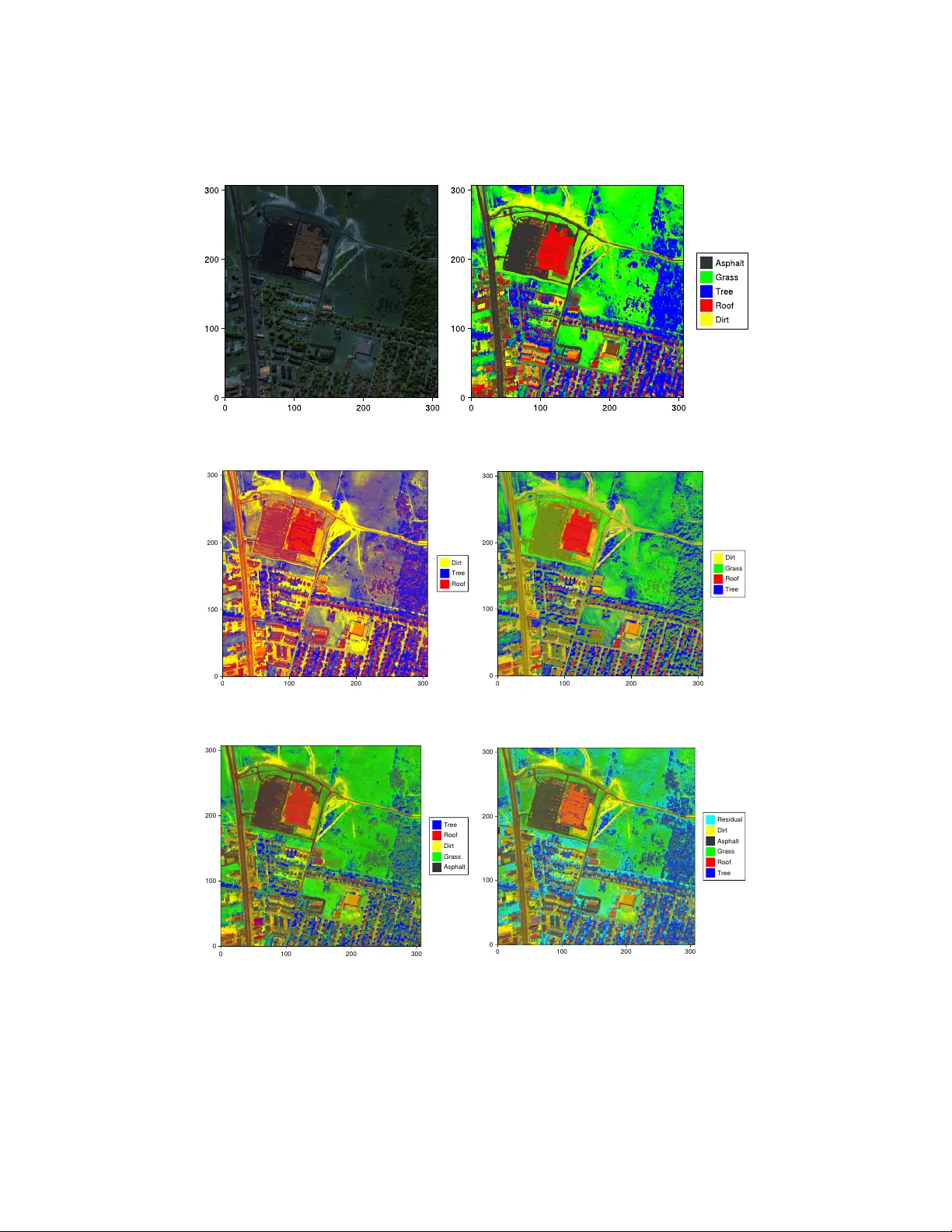
Robust Mo del Selection for Disco v ery of Laten t Mec hanistic Pro cesses Jia w ei Li ∗ 1 , Nguy en Nguy en ∗ 2 , Meng Lai ∗ 3 , Ioannis Ch. P asc halidis 2 , 3 and Jonathan H. Huggins † 1 , 3 1 Dep artment of Mathematics & Statistics, Boston University, USA e-mail: jwli@bu.edu ; huggins@bu.edu 2 Division of Systems Engine ering, Boston University, USA e-mail: nguyenpn@bu.edu ; yannisp@bu.edu 3 F aculty of Computing & Data Scienc es, Boston University, USA e-mail: menglai@bu.edu Abstract: When learning interpretable latent structures using mo del- based approac hes, ev en small deviations from modeling assumptions can lead to inferen tial results that are not mec hanistically meaningful. In this w ork, w e consider laten t structures that consist of K o mec hanistic pro cesses, where K o is unkno wn. When the mo del is missp eciﬁed, likelihoo d-based mo del selection metho ds can substantially ov erestimate K o while more robust nonparametric metho ds can b e ov erly conserv ativ e. Hence, there is a need for approaches that combine the sensitivity of likelihoo d-based metho ds with the robustness of nonparametric ones. W e formalize this ob jectiv e in terms of a r obust mo del sele ction c onsistency property , which is based on a comp onen t-level discrepancy measure that captures the mec hanistic structure of the mo del. W e then prop ose the ac cumulate d cutoﬀ discr ep ancy criterion ( ACDC ), whic h lev erages plug-in estimates of comp onen t-level discrepancies. T o apply ACDC , w e develop mechanisti- cally meaningful comp onent-lev el discrepancies for a general class of latent v ariable models that includes unsupervised and supervised v ariants of prob- abilistic matrix factorization and mixture mo deling. W e show that ACDC is robustly consisten t when applied to unsup ervised matrix factorization and mixture mo dels. Numerical results demonstrate that in practice our approac h reliably identiﬁes a mechanistically meaningful num b er of latent pro cesses in numerous illustrativ e applications, outp erforming existing metho ds. Keyw ords and phrases: Clustering; Latent v ariable mo dels; Mo del selection; Missp eciﬁed mo del; Mixture mo deling; Matrix factorization; Ov erﬁtting. ∗ Equal contribution. † Corresp onding author. 1 J. Li, N. Nguyen, M. L ai, et al./ R obust Mo del Sele ction for Me chanistic Disc overy 2 1. In tro duction Characterizing latent structures with meaningful real-world int erpretations is a common task in scien tiﬁc applications of statistical metho ds. This task often amoun ts to disco v ering unobserv ed ph ysical “pro cesses” that generate observ- able quan tities. F or example, processes might corresp ond to subp opulations that cannot b e directly observ ed suc h as types of cells ( Gorsky , Chan and Ma , 2020 ; Prabhak aran et al. , 2016 ), b ehavioral genotypes ( Stev ens et al. , 2019 ), or groups with canonical patterns of IQ developmen t ( Bauer , 2007 ). Pro cesses could corresp ond to a v ariety of scientiﬁcally imp ortant ob jects suc h cell pro- grams ( Buettner et al. , 2017 ; Kotliar et al. , 2019 ; Risso et al. , 2018 ), mutational pro cesses in tumors ( Kink er et al. , 2020 ; Levitin et al. , 2019 ; Seplyarskiy et al. , 2021 ), or material types ( F´ ev otte and Dobigeon , 2015 ; Ra jabi and Ghassemian , 2015 ). In practice, it is necessary to not only c haracterize each laten t pro cess but also determine how many suc h processes there are. This requires solving a mo del selection problem for a sequence of mo del families M ( K ) = { P θ : θ ∈ Θ K } , K = 1 , 2 , . . . , where K denotes the num b er of latent pro cesses in the mo del. F or example, K could b e the num b er of comp onen ts in a mixture mo del or the n umber of factors in a factor analysis mo del. Giv en some observ ed data x 1 , . . . , x N iid ∼ P o that w ere generated by the output of K o laten t processes, the goal is to recov er K o and a mo del e P o ∈ M ( K o ) suc h that e P o ≈ P o . Likelihoo d- based mo del selection metho ds provide consisten t estimation of K o when M ( K o ) is wel l-sp e ciﬁe d (that is, P o ∈ M ( K o ) but P o / ∈ M ( K ) if K < K o ). Ho w ev er, if M ( K o ) is missp e ciﬁe d (that is, P o / ∈ M ( K o ) ), then these metho ds do not w ork as in tended ( Cai, Campb ell and Bro deric k , 2021 ; F r¨ uh wirth-Sc hnatter , J. Li, N. Nguyen, M. L ai, et al./ R obust Mo del Sele ction for Me chanistic Disc overy 3 2006 ; Guha, Ho and Nguyen , 2021 ; Miller and Dunson , 2019 ; Xue et al. , 2024 ). The reason for this failure is that they optimize for some measure of pr e dictive p erformanc e (e.g., some form of exp ected log loss). Therefore, as N → ∞ , these methods will select a sequence of models that con v erge to the distribution P ⋆ ∈ M ( ∞ ) = S ∞ K =1 M ( k ) that has minimal Kullback–Leibler div ergence b etw een P o and all P ∈ M ( ∞ ) . Since typically P ⋆ / ∈ M ( K ) for an y ﬁnite K , when using a predictive metho d for mo del selection, as the n um b er of observ ations N increases, rather than obtaining b etter estimates, the opposite o ccurs: the distribution P o is better estimated b y adding spurious laten t structures that comp ensate for the shortcomings of the parametric mo del. This problem is known as overﬁtting ( Cai, Campb ell and Broderick , 2021 ). Ho w ev er, when trying discov er real-world pro cesses, the statistical problem is no longer predictive in nature, but rather explanatory ( Shm ueli , 2010 ). The aim is to infer meaningful constructs that capture the underlying causal structure – in this case the laten t pro cesses – even if doing so results in a ﬁtted mo del with reduced predictive p ow er. An alternative set of approaches are nonparametric or semi-parametric in nature. With w eaker assumptions, they can often b e more robust. Ho wev er, b ecause they do not rely on parametric assumptions, they tend to b e less sensitiv e and can (but don’t alw a ys) underestimate the num b er of latent comp onen ts. These nonparametric metho ds also lac k the generalit y of the likelihoo d-based approac hes. Hence, there is a need for robust mo del selection pro cedures that ha v e the generalit y of likelihoo d-based metho ds like Ak aik e, Ba yesian, and deviance information criteria ( Ak aike , 1974 ; Sc h warz , 1978 ; Spiegelhalter et al. , 2002 ) while retaining the robustness to parametric assumptions pro vided by the nonparametric metho ds. Notably , information J. Li, N. Nguyen, M. L ai, et al./ R obust Mo del Sele ction for Me chanistic Disc overy 4 criteria remain widely used due to their simplicity and the ease with whic h they can b e incorp orated in to data analysis w orkﬂows – for example, when a user w ants to use an existing (perhaps sp ecialized) metho d to estimate the parameters of eac h model M ( K ) ( K = 1 , 2 , . . . ). W e defer detailed discussions of related w ork to Sections 2.6 , 3 and 4 . Summary of Con tributions. In this pap er, we make the following con tri- butions to the dev elopment of more reliable and robust methods for mo del selection for disco v ering real-w orld laten t pro cesses: 1. W e deﬁne a formal notion of r obust mo del sele ction c onsistency and argue that it captures key features any robust mo del selection method should satisfy . 2. W e prop ose the ac cumulate d cutoﬀ discr ep ancy criterion ( A CDC ), as a simple, ﬂexible approac h to robust mo del selection. 3. W e sho w how to apply A CDC to a broad class of mo dels in whic h the observ ations are determined b y combining unobserv ed outputs from K laten t pro cesses. 4. W e pro v e that ACDC pro vides robust mo del selection consistency for mixture mo dels and probabilistic matrix factorization mo dels. 5. W e illustrate the adv antages of A CDC through numerical experiments with simulated and real data, including demonstrating state-of-the-art p erformance for cell discov ery using single-cell RNA sequencing data. 1 1 Co de to repro duce all exp erimen ts is av ailable on GitHub: https://github.com/ TARPS- group/robust- model- selection- for- discovery . J. Li, N. Nguyen, M. L ai, et al./ R obust Mo del Sele ction for Me chanistic Disc overy 5 2. Metho dology W e ﬁrst deﬁne robust mo del selection consistency , whic h naturally leads to a plug-in pro cedure, the accum ulated cutoﬀ discrepancy criterion ( ACDC ). W e then describ e ho w to apply A CDC for a broad class of laten t v ariable mo dels. In this section, we use mixture mo deling as a running example to illustrate ideas. Let F = { F ϕ | ϕ ∈ Φ } denote the comp onent distribution family and let η ∈ ∆ K denote the comp onen t w eights, where ∆ K = { η ∈ R K + | P K k =1 η k = 1 } is the ( K − 1)-dimensional probability simplex. Denote the parameter set for the K -comp onen t mixture distributions by Θ ( K ) = ∆ K × Φ K , so the mixture mo del distribution family is M ( K ) = n P θ = P K k =1 η k F ϕ k : θ = ( η , ϕ 1 , . . . , ϕ K ) ∈ Θ ( K ) o . W e can also write the generativ e pro cess of the mixture mo del in terms of laten t v ariables z n ∈ { 1 , . . . , K } that indicate whic h component observ ation n b elongs to: z n | θ ∼ Categorical ( η ) x n | z n = k , θ ∼ F ϕ k . Since w e are in terested in isolating the con tribution of each comp onent, it is this laten t v ariable represen tation that will b e most relev ant. W e discuss applications to other mo dels in Sections 2.3 and 4 . 2.1. R obust Mo del Sele ction Consistency Generalizing the mixture mo del setting, consider a sequence of mo dels M (1) , M (2) , . . . , M ( K ) , . . . , where K captures how man y distinct laten t components are generating the observ ed data. Assume that M ( K ) = { P θ | θ ∈ Θ ( K ) } , where Θ ( K ) is the J. Li, N. Nguyen, M. L ai, et al./ R obust Mo del Sele ction for Me chanistic Disc overy 6 parameter space and P θ ∈ P ( X ), the space of probability measures on the observ ation space X . The ob jectiv e is to identify the true num b er of pro- cesses K o . Fix a distribution-level discr ep ancy D dist on probabilit y measures that will quan tify the ﬁt b etw een P θ and the data-generating distribution P o . W e do not assume a unique minimizing parameter since, at the v ery least, the comp onen t indices in laten t v ariable mo dels are non-identiﬁable. Let Θ ( K ) ⋆ ( P o ) := arg min θ ∈ Θ ( K ) D dist ( P o | P θ ) denote the set of minimizing parameters. Alternatively , a practitioner might c ho ose a parameter estima- tion pro cedure that is not model-based, in which case it might conv erge to a parameter v alue in some other set, whic h w e also denote by Θ ( K ) ⋆ ( P o ). The c hallenge in the missp eciﬁed setting is that for an y θ ( K ) ⋆ ∈ Θ ( K ) ⋆ ( P o ), t ypically D dist ( P o | P θ ( K ) ⋆ ) is not minimized at K = K o . In fact, in our settings of in terest M ( K ) ⊊ M ( K +1) but P o / ∈ M ( K ) for an y K , so D dist ( P o | P θ ( K ) ⋆ ) is monotonically decreasing as K increases. T o correctly reco v er K o , the user m ust specify ho w m uch P θ can deviate from P o while remaining an acceptable appro ximation. Therefore, w e in tro duce a second discrepancy which measures ho w well the c omp onents of P o and P θ matc h. Since the comp onents of P o are unkno wn, the comp onent contributions must b e estimated based on mo del P θ but using the distribution of data from P o . Let the c omp onent-level r e alize d discr ep ancy D ( K ) comp ( θ , k , P o ) quan tify ho w close the inferred comp onen t k ∈ { 1 , . . . , K } from P o is to component k of the model P ( K ) θ . T o quan tify the ov erall degree of comp onen t-lev el missp eciﬁcation of P o with true n um b er of comp onents K o , deﬁne the worst-c ase c omp onent-wise J. Li, N. Nguyen, M. L ai, et al./ R obust Mo del Sele ction for Me chanistic Disc overy 7 discr ep ancy ρ ( P o , K o ) := sup θ ∈ Θ ( K o ) ⋆ ( P o ) max k ∈ [ K o ] D ( K o ) comp ( θ , k , P o ) . F or example, in the mixture mo del case w e can construct a comp onent-lev el realized discrepancy b y inferring the component of P o that would corresp ond to eac h mixture comp onen t. That is, if w e assign each observ ation from P o according to the conditional component probabilities p ( k | x, θ ) = η k d F ϕ k d P θ ( x ), then the inferred k th comp onent of P o is e F ( θ ) ok = p ( k | x, θ ) R p ( k | y , θ ) P o (d y ) P o . Giv en a choice of discrepancy measure D (e.g., D dist ), we can set D ( K ) comp ( θ , k , P o ) = D ( e F ( θ ) ok | F ϕ k ) . Deﬁnition 1 (Robust mo del selection consistency) . Fix a function κ : R + × N → R + . A mo del sele ction pr o c e dur e b K ( x 1: N , ρ ) ∈ N is κ -robustly consistent for Θ ⋆ and D comp if, for any data-gener ating distribution P o and true c omp onent numb er K o that satisﬁes inf θ ∈ Θ ( K ) ⋆ ( P o ) D dist ( P o | P θ ) ≥ κ ( ρ ( P o , K o ) , K ) for al l K ∈ { 1 , . . . , K o − 1 } , (1) it holds that, for x 1 , x 2 , . . . iid ∼ P o , P  b K ( x 1: N , ρ ( P o , K o )) = K o  N →∞ − → 1 . T o in terpret Deﬁnition 1 and the role of the function κ , it is helpful to compare robust mo del selection consistency to classical mo del selection consistency . Figure 1 pro vides a carto on illustration of the diﬀerences. Classical mo del consistency t ypically requires that (1) P o ∈ M ( K o ) and (2) P o / ∈ M ( K ) for J. Li, N. Nguyen, M. L ai, et al./ R obust Mo del Sele ction for Me chanistic Disc overy 8 ℳ 1 ℳ 2 ℳ 3 ℳ K o P C ∘ P B ∘ P D ∘ P A ∘ P E ∘ Fig 1: Carto on illustration of the diﬀerences b etw een traditional and robust mo del selection consistency where the true mo del corresp onds to K o = 4, with the nested mo dels indicated by the gray o v als. W e contrast ﬁv e p ossible data-generating distri- butions, P A o , . . . , P E o , indicated b y the gold p oin ts. Since P A o , P B o ∈ M ( K o ) but are not in M ( K ) for K < K o = 4, for these mo dels K o can b e consisten tly estimated. Ho w ever, since P C o , P D o , P E o / ∈ M ( K o ) , for these distributions K o cannot b e estimated consisten tly in the traditional sense. On the other hand P A o , P B o , P C o , and P D o are close to M ( K o ) , so K o could p otentially b e robustly and consisten tly estimated in these four cases. How ev er, P B o and P D o are also close to M (3) , so robustly consistent estimation of K o is feasible only for P A o and P C o . Since P E o is far from M ( K o ) , K o w ould not b e consistently estimable – either in the traditional or robust sense. K < K o . Robust consistency w eakens the ﬁrst condition b y allowing for a worst- case discrepancy ρ ( P o , K o )  = 0, rather than needing ρ ( P o , K o ) = 0. How ever, robust consistency strengthens the second b y requiring a gap b etw een P o and all mo dels for K < K o . The size of this gap sp eciﬁed in Eq. ( 1 ) in terms of κ . Hence, we call κ the gap function . It would b e natural to ask that κ ( ρ, K ) = ρ , although this ma y not alw a ys be p ossible. 2.2. A Plug-in Pr o c e dur e Inspired b y Deﬁnition 1 , we prop ose a simple plug-in pro cedure for mo del selection,. Assuming ρ o = ρ ( P o , K o ) w ere kno wn, w e w ould w ant to ﬁnd the J. Li, N. Nguyen, M. L ai, et al./ R obust Mo del Sele ction for Me chanistic Disc overy 9 smallest v alue of K suc h that for all k ∈ { 1 , . . . , K } , w e hav e D ( K ) comp ( θ ⋆ , k , P o ) ≤ ρ o for θ ⋆ ∈ Θ ( K o ) ⋆ ( P o ). How ever, since P o and Θ ( K o ) ⋆ ( P o ) are unav ailable, w e prop ose to instead use the empirical distribution b P o = N − 1 P N n =1 δ x n (here δ x denotes the Dirac measure at x ) and a point estimator b θ ( K ) . Hence, w e obtain the plug-in estimator b D ( K,k ) comp = D ( K ) comp ( b θ ( K ) , k , b P o ). Since v alues of b D ( K,k ) comp < ρ o are not important from a mo del selection p ersp ective, w e truncate the estimator b y replacing it with max (0 , b D ( K,k ) comp − ρ ), where ρ is a b est estimate of ρ o . W e can view taking this maxim um as serving a similar role to ho w the coarsened p osterior conditions on the discrepancy having a kno wn upp er b ound. Rather than taking the maximum ov er the comp onen t-wise discrepancy estimates, for b etter robustness to noisy estimates w e use a sum, whic h results in a robust mo del selection loss R ρ ( x 1: n , K ) = K X k =1 max(0 , b D ( K,k ) comp − ρ ) , (2) where for notational simplicity w e ha ve left the dep endence of b D ( K,k ) comp on x 1: n (as a function of b P o and b θ ( K ) ) implicit. Since the loss is the sum (i.e., accumulation) of discrepancies that ha v e b een truncated (i.e., cut oﬀ ) at ρ , we call Eq. ( 2 ) the ac cumulate d cutoﬀ discr ep ancy criterion ( ACDC ). The corresp onding robust mo del estimator is b K ρ ( x 1: n ) = min { arg min K R ρ ( x 1: n , K ) } . Since arg min K ma y return a set of v alues if the loss is equal to zero for more than one v alue of K , it is necessary to include an additional min op eration to select the smallest v alue from the set. W e provide a num b er of metho ds for determining ρ in Section 2.5 . J. Li, N. Nguyen, M. L ai, et al./ R obust Mo del Sele ction for Me chanistic Disc overy 10 y n 1 = f y n 1 = f . . . . . . ϕ 1 ε n 1 ε nK ϕ K z n 1 z nK . . . . . . x n = g ( K ) . . . η w n Fig 2: Graphical represen tation of the general form for mo del M ( K ) for a single observ ation x n . Circles denote random v ariables while squares denote deterministic v ariables. A gray background indicates global parameters while a black bac kground indicates an observed quantit y . 2.3. Mo deling F r amework Guaran teeing robust mo del consistency requires sp eciﬁc c hoices of mo del and comp onen t-level discrepancy . In this pap er, we consider a ﬂexible mo deling framew ork in whic h the observ ed data are the result of K distinct laten t sources (Fig. 2 ). This framework will lead to a natural choice of comp onen t- lev el discrepancy , of which the mixture mo del discrepancy prop osed Section 2.1 is a particular case. W e allo w eac h observ ation x n ∈ X to ha ve sample-sp eciﬁc cov ariates w n ∈ W . Assume that x n dep ends on process-level contributions y n 1 , . . . , y nK ∈ Y via the deterministic function g ( K ) : Y ⊗ K → X : x n = g ( K ) ( y n 1 , . . . , y nK ) . J. Li, N. Nguyen, M. L ai, et al./ R obust Mo del Sele ction for Me chanistic Disc overy 11 F or example, w e could ha ve g ( K ) ( y 1 , . . . , y K ) = P K k =1 y k or g ( K ) ( y 1 , . . . , y K ) = max k y k . The pro cess-level con tributions are in turn determined by an observ ation- sp eciﬁc latent v ariable z n = ( z n 1 , . . . , z nK ) ∈ Z ( K ) ⊆ Z ⊗ K and the pro cess- sp eciﬁc parameters ϕ 1 , . . . , ϕ K ∈ Φ. W e assume b oth Y and Z con tain a nul l value ∅ , which indicates no con tribution. Speciﬁcally , w e assume g ( K ) has the follo wing no c ontribution pr op erty : for all y 1 , . . . , y K − 1 ∈ Y , g ( K ) ( y 1 , . . . , y K − 1 , ∅ ) = g ( K − 1) ( y 1 , . . . , y K − 1 ) . Giv en a deterministic function f : W × Z × Φ × R → Y and indep endent noise random v ariables ε nk iid ∼ G , the comp onent-lev el con tributions are giv en b y y nk =        ∅ , if z nk = ∅ , f ( w n , z nk , ϕ k , ε nk ) , otherwise . If there are no cov ariates, we drop the dep endence on w n and write f ( z nk , ϕ k , ε nk ) instead. T ypically Z ⊆ R and z nk represen ts the activit y lev el of the k th process for the n th observ ation. In such cases, usually ∅ = 0. F or a global parameter η ∈ E ( K ) , we assume the observ ation-sp eciﬁc laten t v ariables are indep endent but may dep end on the sample-speciﬁc co v ariates: z n | η , w n ind ∼ H ( K ) η ,w n . If there are no cov ariates, we drop the dep endence on w n and write H ( K ) η instead. Our framework captures man y common mo del t yp es: Example 1 (Mixture Mo deling) . We c an r e c over a gener al mixtur e mo del by taking H ( K ) η = Catego rical ( η ) , so z nk ∈ { 0 , 1 } and P K k =1 z nk = 1 . Given a J. Li, N. Nguyen, M. L ai, et al./ R obust Mo del Sele ction for Me chanistic Disc overy 12 mixtur e c omp onent distribution family F = { F ϕ | ϕ ∈ Φ } , deﬁne f such that, for ε ∼ G , it holds that f (0 , ϕ, ε ) = 0 and f (1 , ϕ, ε ) ∼ F ϕ . Final ly, take g ( K ) to b e the summation op er ator. Henc e, if z nk = 1 , then x n = y nk ∼ F ϕ k . Example 2 (Mixture Mo del with V arying Component Probabilities) . When c ovariates ar e available for e ach observation, the mixtur e mo del c an b e gen- er alize d to al low the mixtur e pr ob abilities to dep end on observe d c ovariates ( Huang and Y ao , 2012 ; Jasp ers, Kom´ ar ek and A erts , 2018 ). We c an r e- c over this mo del by using the same setup as Example 1 but inste ad letting H ( K ) η ,w n = Catego rical ( h ( η , w n )) for some ﬁxe d function h : E ( K ) × W → ∆ K . Example 3 (Probabilistic Matrix F actorization) . F or pr ob abilistic matrix factorization (PMF), x n ∈ R D . L et Z ⊆ R and Φ ⊆ R D . We assume that F = { F µ | µ ∈ R D } is a lo c ation family of distributions satisfying R xF µ (d x ) = µ for al l µ ∈ R D . L et f satisfy f ( z , ϕ, ε ) ∼ F z ϕ if ε ∼ G . F or example, in nonne gative matrix factorization, F µ = P oiss ( µ ) while in classic al factor analysis F µ = N ( µ, σ 2 ) , wher e σ 2 c an also b e le arne d. Final ly, take g ( K ) to b e the summation op er ator. Our framew ork is similarly applicable to sup ervised v arian ts of probabilistic matrix factorization models, functional clustering problems, and a v ariety of other latent v ariable mo dels ( Blei and Laﬀert y , 2007 ; Carv alho et al. , 2008 ; Chiou and Li , 2007 ; Cunningham and Y u , 2014 ; Dunson , 2000 ; W est , 2003 ). 2.4. Constructing the Comp onent-level Discr ep ancy T o deﬁne the comp onen t-lev el discrepancy , it is tempting to directly apply the approac h w e to ok for mixture models and quan tify the diﬀerence b et ween the J. Li, N. Nguyen, M. L ai, et al./ R obust Mo del Sele ction for Me chanistic Disc overy 13 distributions of y n 1 , . . . , y nK when x n ∼ P o and the mo deled distributions of y n 1 , . . . , y nK . Ho w ev er, the distributions of y 1 k , y 2 k , . . . , y nk , . . . ma y b e diﬀerent due to the sample-sp eciﬁc dependence on w n and z nk . T o address this issue, we instead consider the discrepancy b etw een the conditional distribution of the noise v ariables ε nk giv en x 1: N and the assumed noise distribution G . How ever, w e m ust exclude ε nk if y ( K ) nk = ∅ b ecause then it is no longer part of the graphical mo del (see Fig. 2 ). Dropping the dep endence on n , the inferred distribution of the k th noise v ariable is e G ( θ ) k = Z L ( ε k | y k  = ∅ , x, w , θ ) P o (d x, d w ) , where L ( ε k | · · · ) denotes a conditional law of ε k . Hence, deﬁne the discrepancy for the k th component b y D ( K ) comp ( θ , k , P o ) = D ( e G ( θ ) k | G ). T o deﬁne an empirical version of D ( K ) comp ( θ , k , P o ), let b G ( K ) nk = L ( ε nk | x n , w n , b θ ( K ) ), deﬁne the usage indicators u ( K ) nk = 1 ( y ( K ) nk  = ∅ ), and denote the num b er of obser- v ations for comp onent k as N ( K ) k = P N n =1 u ( K ) nk . Then the empirical distribution of the noise v ariables for comp onent k is b G ( K ) k = 1 N ( K ) k N X n =1 u ( K ) nk b G ( K ) nk . Hence, an estimate of discrepancy for the k th comp onent is given by b D ( K,k ) comp = D ( b G ( K ) k | G ) . (3) In some scenarios, it is necessary to replace the div ergence with an estimator b ecause D ( b G ( K ) k | G ) is undeﬁned (e.g., the KL div ergence) or not eﬃcien tly computable (e.g., the W asserstein distance). In Section F , we discuss ho w b est to estimate the KL div ergence in practice and provide supp orting consistency J. Li, N. Nguyen, M. L ai, et al./ R obust Mo del Sele ction for Me chanistic Disc overy 14 theory b y mo difying the t w o-sample KL div ergence estimation theory developed in W ang, Kulk arni and V erd ´ u ( 2009 ) to the one-sample estimation setting applicable to A CDC . In Section G.1 , w e discuss using the en trop y-regularized W asserstein distance (the Sinkhorn distance) as a stable, eﬃciently computable alternativ e to the W asserstein distance that scales to high dimensions. 2.5. Cho osing ρ The v alue of ρ is problem dependent, as it quantiﬁes the maximum amount of mo del missp eciﬁcation of each pro cess. W e prop ose t wo complementary approac hes to selecting ρ that take adv an tage of the fact that the robust loss is a piecewise linear function of ρ . Therefore, given a ﬁtted mo del for each candidate K , we can easily compute the loss for all v alues of ρ . Using domain knowledge. The ﬁrst approac h aims to lev erage domain kno wledge. Sp eciﬁcally , it is frequen tly the case that some related datasets are av ailable with “ground-truth” lab els either through manual lab eling or via in silic o mixing of data where group lab els are directly observed (see, e.g., de Souto et al. , 2008 ). In suc h cases, an empirically optimal ρ v alue for one or more suc h datasets with ground-truth lab els can b e determined b y maximizing a problem-appropriate accuracy metric such as F-measure. Because ρ quan tiﬁes the div ergence b etw een the true pro cess distributions and the mo del estimates, w e exp ect the v alues found using this approach will generalize to new datasets that are reasonably similar. W e illustrate this approac h in Section 3.2 . Alternativ ely , if real data with ground truth K o is una v ailable, plausible sim ulated data could b e used to calibrate ρ instead ( Xue et al. , 2024 ). J. Li, N. Nguyen, M. L ai, et al./ R obust Mo del Sele ction for Me chanistic Disc overy 15 A generally applicable approach. F or applications where there are no related datasets with ground-truth lab els av ailable, w e prop ose a second ap- proac h. After estimating the mo del parameters for each ﬁxed K and computing all pro cess-wise divergences, w e plot the loss as a function of ρ for each K ∈ { K min , . . . , K max } . F or readabilit y , in tro duce a small p ositive constan t λ ≪ 1 and plot R ρ ( x 1: N , K ) + λK so it is p ossible to distinguish the lines when the loss is exactly zero. The optimal model is determined by iden tifying the n um b er of pro cesses whic h is b est o ver a substan tial range of ρ v alues, with ρ as small as p ossible. The idea b ehind this selection rule is to identify the ﬁrst instance of stability , indicating that allo wing just a small amoun t of additional missp eciﬁcation (by increasing ρ ) do esn’t notably improv e the loss. How ever, subsequen t stable regions that app ear afterward migh t in tro duce to o m uc h tolerance, p oten tially resulting in mo del underﬁtting. This approac h is similar in spirit to the one in tro duced for heuristically selecting the α parameter for the coarsened p osterior ( Miller and Dunson , 2019 ). Automation. Building on the same heuristic intuition, we can automate the selection of ρ b y deﬁning a minim um width ∆ min for whic h an in terv al can b e recognized as the stabilit y region. Sp eciﬁcally , w e keep trac k of the smallest ρ v alue, ρ start , for whic h a K -sp eciﬁc penalized loss b ecomes minimal among all other K -sp eciﬁc losses. W e then iden tify the next ρ v alue, ρ end , at whic h this same loss curv e is no longer the minimum. The diﬀerence b et w een ∆ = ρ end − ρ start deﬁnes an interv al of stability . If ∆ ≥ ∆ min (i.e., ∆ has the predeﬁned minim um width), it is recognized as a stabilit y in terv al, the corresp onding v alue of K is chosen to b e b K . Otherwise, ρ end b ecomes ρ start and rep eat the pro cedure to compute the new ρ end and ∆, c heck if ∆ ≥ ∆ min , and so J. Li, N. Nguyen, M. L ai, et al./ R obust Mo del Sele ction for Me chanistic Disc overy 16 forth. The v alue of ∆ min should be set based on preliminary manual exp eriments to estimate a suitable stabilit y region width for automated selection in larger batc hes. This approach allo ws users to adjust the interv al threshold to balance the tradeoﬀ b et ween a v oiding underﬁtting (∆ min suﬃcien tly small) and ensuring appropriately conserv ative and stable mo del selection (∆ min suﬃcien tly large). W e demonstrate the utility of this approac h in Section 3.3 . 2.6. R elate d Work There is limited w ork on general-purp ose approac hes to robust mo del selection with the goal of ensuring interpretabilit y . Recent w ork on robustifying likeli- ho o ds to small model p erturbations oﬀer one promising strategy ( Chakrab orty , Bhattac hary a and Pati , 2023 ; Dew ask ar et al. , 2023 ; W u et al. , 2024 ). Ho wev er, these metho ds aim to replace existing parameter estimation metho ds rather than augment them – which is a k ey goal of the present wo rk. P erhaps most closely related to our work is Miller and Dunson ( 2019 ), whic h prop oses an elegan t robust Ba y esian mo del selection pro cedure that emplo ys a tec hnique they call c o arsening . Unlik e the standard posterior, whic h assumes the data w ere generated from the assumed mo del (that is, it conditions on x = x obs ), the c o arsene d p osterior conditions on the “true mo del data” b eing close to the observ ed data (that is, it conditions on the estimated Kullback–Leibler diver- gence b et ween x and x obs b eing less than some threshold γ ) – hence, sacriﬁcing predictiv e p ow er for greater robustness. Ho wev er, using the coarsened p osterior approac h has a p otentially high computational cost b ecause it requires running Mark o v chain Mon te Carlo dozens of times to heuristically determine a suitable robustness threshold ( Miller and Dunson , 2019 ; Xue et al. , 2024 ). In addition, J. Li, N. Nguyen, M. L ai, et al./ R obust Mo del Sele ction for Me chanistic Disc overy 17 our exp eriments sho w that, while coarsening oﬀers go o d robustness in many scenarios, it do es not ha v e ha ve any formal correctness guaran tees and can fail in simple situations (see Section G.2 ). 3. Application to Mixture Mo dels In the next t w o sections, we illustrate the use of A CDC in some represen tativ e applications while also providing theoretical supp ort for our approac h b y sho wing that ACDC is robustly consisten t. F or readabilit y , theorems are stated informally in the main text. F ormal statemen ts of assumptions and results are deferred to Section A . F or all exp erimen ts, unless stated otherwise we use the KL divergence as the discrepancy measure D for the calculation of the estimated component-lev el discrepancy b D ( K,k ) comp deﬁned in Eq. ( 3 ). W e compare to BIC since, lik e A CDC , it only requires a p oint estimate for eac h v alue of K . Alternative criteria lik e AIC and DIC w ould giv e similar results. Ho wev er, since BIC has a larger p enalt y than AIC (which DIC generalizes), it will b e more conserv ativ e and hence tend to choose smaller v alues of K . See, for example, Cai, Campbell and Bro deric k ( 2021 ); Miller and Dunson ( 2019 ); Xue et al. ( 2024 ) for numerical examples sho wing that Bay esian mo del selection do es not resolv e the ov erﬁtting problem. In this section, w e consider mixture mo deling, for which ACDC is robustly consisten t: Theorem 1. A CDC using b D ( K,k ) comp deﬁne d in Eq. ( 3 ) is κ -r obustly c onsistent for mixtur e mo dels if the underlying c omp onent discr ep ancy D is the KL diver genc e, Wasserstein distanc e, or maximum me an discr ep ancy (MMD). F or the KL diver genc e, κ ( ρ, K ) = √ ρ and D dist = d BL , the b ounde d Lipschitz distanc e. F or J. Li, N. Nguyen, M. L ai, et al./ R obust Mo del Sele ction for Me chanistic Disc overy 18 Wasserstein distanc e and MMD, κ ( ρ, K ) = ρ and D dist = D . In addition to BIC, we compare ACDC to three nonparametric, mixture mo del-sp eciﬁc selection metho ds that rely on within-cluster disp ersion. F or K clusters, the total within-cluster sum of squar es WCSS( K ) is deﬁned as W CSS( K ) = K X k =1 X x ∈ C k ∥ x − µ k ∥ 2 , where C k is the set of observ ations assigned to cluster k and µ k is its cen troid. The ﬁrst approach is the elb ow metho d , whic h identiﬁes the p oint b eyond whic h additional clusters no longer show signiﬁcan t impro vemen t in dispersion reduction ( Thorndike , 1953 ). The silhouette c o eﬃcient , on the other hand, assesses how well eac h p oint ﬁts within its assigned cluster relativ e to its distance to the nearest neighboring cluster ( Rousseeuw , 1987 ). It fav ors clusters with high cohesion where p oin ts are close to others in the same cluster, and high separation where clusters are w ell isolated from one another. Finally , the gap statistic compares the observed clustering disp ersion in the data to what is exp ected under a n ull reference where data comes from uniform distribution ( Tibshirani, W alther and Hastie , 2001 ). The selection is based on the n um b er of clusters that maximizes the deviation from its baseline. F or all mixture mo del exp eriments, w e use the EM algorithm to obtain parameter estimates. Unless stated otherwise, we use the bias-corrected KL estimator for A CDC (see Section F for details). Giv en estimates ˆ K 1 , . . . , ˆ K T for T datasets with true K v alues of, respectively , K 1 , . . . , K T , we measure p erformance in terms of the mean absolute deviation MAE = T − 1 P T t =1 | ˆ K t − K t | , the mean 0-1 loss 0-1 = T − 1 P T t =1 1 ( ˆ K t  = K t ), and the median of the signed deviations { ˆ K t − K t } T t =1 . J. Li, N. Nguyen, M. L ai, et al./ R obust Mo del Sele ction for Me chanistic Disc overy 19 3.1. Simulation Study W e ﬁrst in vestigate the accuracy of A CDC under a v ariet y of conditions on the level of missp eciﬁcation, the relativ e sizes of the mixture comp onen ts, and the data dimension. W e generate data x 1 , . . . , x N ∈ R D from the mixture distribution P o = P K o k =1 η ok S N ( m ok , Σ ok , γ ok ), where S N ( m, Σ , γ ) denotes a sk ew normal distribution with lo cation v ector m ∈ R D , scale matrix Σ ∈ R D × D , and shap e γ ∈ R D , which controls the sk ewness. When D > 1, we introduce w eak correlations b y letting Σ ok = Σ, where Σ ij = exp {− ( i − j ) 2 /σ 2 } and σ con trols the strength of the correlation. See Section H.1 for full exp erimen tal details. High-dimensional data. W e suggest using the KL divergence as a default discrepancy c hoice. But, as discussed in Section F , the k -nearest-neigh b or estimator b ecomes less accurate with increasing data dimension. While a general solution is unlikely to exist, we illustrate one approach to address this challenge. Sp eciﬁcally , if w e b eliev e the co ordinates are lik ely to be only w eakly correlated, w e can emplo y the k -nearest-neigh b or metho d on each co ordinate by assuming the co ordinates are indep enden t. W e set D = 25, N = 10 000, K o = 3, and σ = 0 . 6. As sho wn in Fig. 3 (left), the wide and stable region corresp onds to the true correct n umber of comp onen ts. Fig. 3 (righ t) illustrates the v alue of mo del-based clustering, particularly in high dimensions: 2-dimensional pro jections of the data give the app earance of there b eing four clusters in total, when in fact there are only three. Comparison to other metho ds. T o assess the relative p erformance of A CDC , w e compare it to the three nonparametric mo del selection metho ds. J. Li, N. Nguyen, M. L ai, et al./ R obust Mo del Sele ction for Me chanistic Disc overy 20 0.0 0.2 0.4 0.6 0.8 1.0 1 0 2 1 0 1 P enalized loss X K = 3 K=1 K=2 K=3 K=4 Fig 3: Application of A CDC clustering simulated high dimensional data (Section 3.1 ). Left: The p enalized loss plot for K ∈ { 1 , 2 , 3 , 4 } . Since the loss for K = 3 is v ery close to equal to or m uch less than the loss for K  = 3, it shows the greatest stabilit y , resulting in b K = 3 (indicated b y the “ X ”). Righ t: Selected t w o-dimensional pro jections of the data. In the low-dimensional setting ( D ∈ { 2 , 3 } ), A CDC achiev es the best ov erall p erformance, with the smallest MAE of 0 . 20 and mean 0–1 loss of 0 . 18, and a median deviation equal to zero (Fig. 4a ). By con trast, the competing metho ds exhibit MAE v alues of ≥ 0 . 60 and mean 0–1 losses of ≥ 0 . 40. Both the elb ow and silhouette criteria sho w a tendency to underestimate the num b er of comp onen ts. The gap statistic sho ws the highest v ariability and signiﬁcan t underestimation. In the high-dimensional setting (Fig. 4b ), A CDC has similar p erformance to the silhouette criteria while signiﬁcantly outp erforming the elb ow and gap metho ds, particularly in terms of MAE. F or the low and high-dimensional settings, all diﬀerences b et w een the MAE v alues of A CDC and the three alternativ e metho ds w ere statistically signiﬁcan t except for A CDC versus the silhouette co eﬃcien t applied to the high-dimensional data (Wilco xon signed-rank test; see T able H.1 for exact p-v alues). J. Li, N. Nguyen, M. L ai, et al./ R obust Mo del Sele ction for Me chanistic Disc overy 21 Elbow Gap Silhouette A CDC Method 3 2 1 0 1 K K o MAE = 0.63 0-1 = 0.58 MAE = 0.65 0-1 = 0.40 MAE = 0.70 0-1 = 0.57 MAE = 0.20 0-1 = 0.18 (a) low-dimensional Elbow Gap Silhouette A CDC Method 6 4 2 0 2 K K o MAE = 0.72 0-1 = 0.42 MAE = 0.62 0-1 = 0.30 MAE = 0.28 0-1 = 0.25 MAE = 0.25 0-1 = 0.25 (b) high-dimensional Fig 4: Comparison of A CDC with common mo del selection criteria (Elb ow, Gap, and Silhouette) in low-and high-dimensional settings. Eac h p oint shows the deviation b et ween estimated and true cluster counts ( ˆ K − K o ) of one dataset. Dotted black lines indicate the median error for each metho d. Mean absolute error (MAE) and 0–1 loss quantify the mo del selection accuracy . 3.2. Cel l T yp e Disc overy using Flow Cytometry As a ﬁrst inv estigation of ACDC applied to real data, we follow the setup of Miller and Dunson ( 2019 ) using 12 ﬂow cytometry datasets originally from a longitudinal study of graft-versus-host disease in patien ts undergoing blo o d marro w transplantation ( Brinkman et al. , 2007 ). Flow cytometry is a technique used to analyze prop erties of individual cells in a biological material ( McKinnon , 2018 ). T ypically , ﬂo w cytometry data consists of 3–20 prop erties of tens of thousands cells. Cells from distinct p opulations tend to fall in to clusters and disco v ering cell types b y iden tifying clusters is of primary in terest in practice. Usually scientists identify clusters manually , whic h is lab or-in tensive and sub- jectiv e. Therefore, clustering metho ds that provide interpretable groups of cells is in v aluable. Nev ertheless, for our exp eriments we treat the man ual cluster assignmen ts as the ground truth, which w as feasible b ecause the datasets ha ve J. Li, N. Nguyen, M. L ai, et al./ R obust Mo del Sele ction for Me chanistic Disc overy 22 0 1 2 3 4 5 0.6 0.7 0.8 0.9 1.0 F-measur e 1 . 1 6 Fig 5: Selecting an optimal v alue of ρ using the ﬁrst 6 ﬂow cytometry datasets (Section 3.2 ). The solid lines show ρ vs. F-measure for datasets 1–6. The black dashed line indicates a v eraged F-measure ov er the training datasets. The vertical blac k line sho ws the v alue ρ = 1 . 16 that maximizes the av eraged F-measure. dimension D = 4. T o calibrate ρ , w e follo w the domain kno wledge-aided approac h describ ed in Section 2.5 . F or comparability with the results of Miller and Dunson ( 2019 ), w e use F-measure to quan tify clustering accuracy and calibrate ρ using the ﬁrst 6 datasets. As sho wn in Fig. 5 , the training datasets 1–6 ha v e a nearly iden tical trend of clustering accuracy as a function of ρ . The av eraged F- measure achiev es the maximum when ρ ≈ 1 . 16, which is a p oin t of maxim um F-measure for all 6 datasets. The consistency of ACDC compares fa vorably to using coarsening, where drastically diﬀerent α v alues maximize the F-measure ( Miller and Dunson , 2019 , Figure 5). These results provide evidence that our approac h is taking b etter adv antage of the common structure and degree of missp eciﬁcation across datasets. F or test datasets 7–12, w e pic k the v alue of K based on a v alue of ρ that is as close as p ossible to the estimated ρ v alue of 1 . 16 while also b eing stable for a J. Li, N. Nguyen, M. L ai, et al./ R obust Mo del Sele ction for Me chanistic Disc overy 23 T able 1 F-me asur es on ﬂow cytometry test datasets 7–12 7 8 9 10 11 12 A CDC 0.63 0.92 0.94 0.99 0.99 0.98 Coarsened 0.67 0.88 0.93 0.99 0.99 0.99 Elb o w 0.91 0.91 0.93 0.99 0.99 0.98 Gap 0.73 0.91 0.93 0.99 0.98 0.98 Silhouette 0.63 0.74 0.94 0.99 0.96 0.98 range of ρ v alues. As sho wn in T able 1 , A CDC provides the same av erage accuracy as the coarsened p osterior while b eing substantially more computationally eﬃcien t, despite using a m uch slow er programming language for implemen tation ( A CDC to ok 2 hours using Python while the coarsened p osterior to ok 30 hours using Julia). A CDC performs comparably to the nonparametric metho ds, although the elb o w method p erforms the b est, particularly on dataset 7. 3.3. Cel l T yp e Disc overy using Single-Cel l RNA Se quencing Data There are t w o limitations to our ﬂow cytometry exp erimen ts: the cell types are based on manual lab eling (whic h ma yb e be incorrect) and the data is low dimensional. T o more fully test the capabilities of ACDC on high-dimensional datasets with reliable ground truth, we consider the common task of identifying cell types from single-cell RNA sequencing (scRNA-seq) data. Current practice relies hea vily on heuristics to determine the n um b er of cell types, whic h are kno wn to b e inaccurate ( Grabski, Street and Irizarry , 2023 ). W e ev aluate A CDC and the alternative metho ds on the T abula Muris dataset ( Consortium , 2018 ), which proﬁles nearly 100,000 mouse cells across 20 tissues with curated ground-truth cell types. W e applied all metho ds to 80 data subsets with equally sized clusters (see T able H.2 ). All datasets undergo the same prepro cessing steps described in Section H.3 . F ollowing common practice, J. Li, N. Nguyen, M. L ai, et al./ R obust Mo del Sele ction for Me chanistic Disc overy 24 0 2 4 6 8 −4 0 4 8 K ^ − K o Frequency 0 2 4 6 −6 −4 −2 0 2 4 K ^ − K o Frequency 0 5 10 15 20 0 5 10 15 20 K o K ^ Distance Metric KL Sinkhorn Fig 6: Comparison of KL to Sinkhorn as div ergence estimators for scRNA-seq clustering. Diﬀerence in K estimates using ACDC with KL div ergence (left) and W asserstein distance (middle . The dashed v ertical lines indicate the medians. Righ t: T rue num b er of cell types vs. estimated num b er of cell types (jittered). w e use log-transformed gene expression coun ts and ﬁt a Gaussian mixture mo del. The mo del is clearly missp eciﬁed, motiv ating the need for a robust clustering approach. The cell clustering p erformance is assessed b y (1) the accuracy of estimating the true n umber of cell types and (2) the agreement b et ween estimated and true lab els, quan tiﬁed using using the Adjusted Rand Index (ARI) and Adjusted Mutual Information (AMI) ( Hub ert and Arabie , 1985 ; Vinh, Epps and Bailey , 2010 ). Discrepancy Choice. One b eneﬁt of ACDC is that the user can select a discrepancy measure D that best captures the underlying structure of their data. While the KL divergence is our recommended default, the W asserstein distance can b etter align with the underlying metric structure of the data. In single- cell clustering, the cosine distance captures directional relationships b etw een gene expression proﬁles. This is particularly useful with high-dimensional scRNA-seq data where the magnitude of total gene counts in each cell can v ary signiﬁcan tly , while the expression prop ortions across genes remain informative. W e use the unbalanced Sinkhorn distance to estimate the W asserstein distance J. Li, N. Nguyen, M. L ai, et al./ R obust Mo del Sele ction for Me chanistic Disc overy 25 (see Section H for details). As illustrated in Fig. 6 , b oth choices of discrepancy lead to goo d estimates of the true num b er of cell types, with the KL v ersion ha ving a slight bias tow ard o verestimation (median diﬀerence of 2 from the ground-truth K o ) and the W asserstein version sho wing a slight bias to w ard underestimation (median diﬀerence of − 1). These results demonstrate the robustness of our default choice (KL divergence), while also highligh ting the b eneﬁts of b eing able to improv e p erformance by making a problem-sp eciﬁc c hoice (the W asserstein distance). F or consistency with our other experiments, w e contin ue to use the KL div ergence for the remaining exp erimen ts. Automation. T o facilitate large-scale analyses and reduce man ual in terven- tion, w e also assess the automated selection of the regularization parameter ρ using the stabilit y-based procedure in tro duced in Section 2.5 . As sho wn in Fig. H.5 , the man ually selected K ac hiev es sligh tly b etter ARI v alues (ranging from − 0 . 27 to 0 . 37), while automated K selection results in higher AMI v alues (ranging from − 0 . 19 to 0 . 33). T o assess whether the diﬀerences are signiﬁcan t, w e conduct paired t-tests on the AMI and ARI scores. F or AMI, the mean diﬀerence betw een the tw o metho ds is 0 . 0027 (95% CI: [ − 0 . 0095 , 0 . 0148]). F or ARI, the mean diﬀerence is 0 . 0084 (95% CI: [ − 0 . 0069 , 0 . 0237]). In terms of estimation accuracy , man ual tuning of ρ yields sligh tly lo w er mean absolute error (MAE = 2 . 16 vs. 2 . 43) and 0–1 loss (0 . 84 vs. 0 . 88) compared to the automated approac h. The mean diﬀerence in absolute error b etw een the man ual and the automated pro cedures ( | ˆ K manual − ˆ K auto | ) is − 0 . 26 (95% CI: [ − 0 . 57, 0 . 05]). Overall, the diﬀerence b etw een the automated and manual approac hes – in terms of b oth clustering accuracy and estimation accuracy – is minimal. J. Li, N. Nguyen, M. L ai, et al./ R obust Mo del Sele ction for Me chanistic Disc overy 26 A CDC Elbow Silhouette Gap Seurat SC3 Method 20 0 20 40 60 K K o MAE = 2.40 0-1 = 0.85 MAE = 3.36 0-1 = 0.91 MAE = 5.51 0-1 = 0.94 MAE = 5.78 0-1 = 0.91 MAE = 7.21 0-1 = 1.00 MAE = 31.23 0-1 = 1.00 Fig 7: Comparison of A CDC with common mo del selection criteria (Elb o w, Gap, and Silhouette) and sp ecialized to ols for scRNA-seq clustering (Seurat and SC3) on 80 scRNA-seq datasets. Eac h p oint shows the deviation b etw een estimated and true n umbers of cell t yp es ( ˆ K − K o ). Dotted blac k lines indicate the median error for eac h metho d. Mean absolute error (MAE) and 0–1 loss quantify the mo del selection accuracy . Comparison to other metho ds. There are a n um b er of specialized to ols for scRNA-seq clustering. So, in addition to comparing A CDC to Elb ow, Gap, and Silhouette (all applied to the same parameter estimates), we also b enc hmark t w o widely used scRNA-seq clustering pip elines, Seurat ( Butler et al. , 2018 ) and SC3 (Single-Cell Consensus Clustering; Kiselev et al. , 2016 ); see Section H.5 for further details ab out these tools. As sho wn in Fig. 7 , A CDC ac hieves the b est cluster estimation accuracy (MAE = 2 . 40, 0–1 loss = 0 . 85). T o quan tify the diﬀerence in estimation accuracy , w e conduct paired t-tests on the absolute estimation errors b etw een A CDC and each comp eting metho d. The mean diﬀerences in absolute error b et ween ACDC and comp eting methods are − 0 . 96 for Elb ow (95% CI: [ − 1 . 59, − 0 . 33]), − 3 . 11 for Silhouette (95% CI: [ − 3 . 97, − 2 . 26]), − 3 . 38 for Gap (95% CI: [ − 4 . 41, − 2 . 34]), − 4 . 81 for Seurat (95% CI: [ − 5 . 50, − 4 . 12]), and − 28 . 83 for SC3 (95% CI: [ − 31 . 28, − 26 . 37]), indicating J. Li, N. Nguyen, M. L ai, et al./ R obust Mo del Sele ction for Me chanistic Disc overy 27 A CDC outp erforms all other metho ds. In terms of estimation bias, the gap (median = 3 . 0) and silhouette (median = 6 . 0) criteria exhibit a stronger tendency to ov erestimate the num b er of clusters, while the elb ow metho d (median = − 2 . 0) tends to underestimate. All three metho ds show median deviations farther from zero than those of ACDC (median = 1 . 0). Seurat (median = 7 . 0) pro duces consisten tly inﬂated estimates and SC3 (median = 32 . 5) substantially ov ersho ots K o in all datasets. In terms of clustering agreemen t, A CDC remains highly comp etitiv e, ac hieving ARI and AMI v alues comparable to Seurat (see Fig. H.7 ). 4. Application to Probabilistic Matrix F actorization Next, we apply ACDC to probabilistic matrix factorization problems. As with mixture mo dels, A CDC is robustly consistent: Theorem 2. A CDC using b D ( K,k ) comp deﬁne d in Eq. ( 3 ) is κ -r obustly c onsistent for pr ob abilistic matrix factorization if the underlying c omp onent discr ep ancy D is the KL diver genc e, D dist = d BL , and κ ( ρ, K ) = p K ρ/ 2 . In our n umerical experiments, we take G = Unif ([0 , 1] D ), the uniform distri- bution on the D -dimensional hypercub e. This c hoice is without loss of generalit y when using KL divergence as the discrepancy measure since it is inv ariant to diﬀeomorphisms of the noise v ariables ε nk . Moreo v er, it leads to a univ ersal c hoice of f ( z , ϕ, · ) = F − 1 z ϕ , the in v erse CDF. Ho wev er, in sp eciﬁc scenarios other c hoices for G and f migh t b e preferred due to considerations suc h as ease of implemen tation or stabilit y of KL divergence estimation. F or example, in the Gaussian case, w e could tak e G = N (0 , I ) and f ( z , ϕ, ε ) = z ϕ + σ ε . J. Li, N. Nguyen, M. L ai, et al./ R obust Mo del Sele ction for Me chanistic Disc overy 28 𝜌 0 5 10 𝓡 𝜌 10 − 1 10 0 10 1 K 1 2 3 4 5 6 7 8 9 1 0 1 1 12 13 14 15 ma x D r a d 1 0 0.0 1 0 0.5 1 0 1.0 1 2 3 4 5 6 7 8 9 1 0 1 1 12 13 14 15 m a x D cos 0. 0 0. 5 1. 0 K 1 2 3 4 5 6 7 8 9 1 0 1 1 12 13 14 15 B I C ( × 1 0 6 ) 0. 6 0. 9 1. 2 K 1 2 3 4 5 6 7 8 9 1 0 1 1 12 13 14 15 E i g e n va l u e s 0 1.0 × 10 ⁵ 2.0 × 10 ⁵ 3.0 × 10 ⁵ 4.0 × 10 ⁵ K=1 K=2 K=3 K=4 K=5 K=6 K=7 K=8 K=9 K=10 K= 1 1 K=12 K= 1 3 K=14 K= 1 5 A c tual Eigen v alues Random Eigen v alues BIC PA ACDC Fig 8: Estimation quality of m utational signature disco very for p erturb ed syn thetic breast cancer data (Section 4.1 ). (top) Errors of signature and loadings estimates. (middle top) K v ersus v alue of BIC. BIC selects b K = K max . (middle b ottom) Scree plot generated from the dataset, indicating that K = 2 is the optimal choice of K . (b ottom) Structurally aw are loss for K ∈ { 1 , . . . , K } , the wide region with the smallest ρ is mark ed b y the cross mark, indicating K = 7 or K = 8 is the most appropriate choice of K . J. Li, N. Nguyen, M. L ai, et al./ R obust Mo del Sele ction for Me chanistic Disc overy 29 In addition to BIC, w e compare ACDC to p ar al lel analysis (P A) ( Buja and Eyub oglu , 1992 ; Horn , 1965 ), which is a commonly used nonparametric metho d for mo del selection for probabilistic matrix factorization. Parallel analysis is carried out b y generating the scree plot (ordered PCA eigenv alues) of the data against that of randomly generated matrices of the same size. These random matrices are generated by indep enden tly p erm uting each ro w of the data matrix. The results of Dobriban ( 2020 ) show that, in general, P A can b e conserv ative and miss factors with a low signal-to-noise ratio. F or BIC, to accoun t for p erm utation in v ariance of the parameters, we use the form ula BIC  x 1: N , z ( K ) 1: K, 1: N , ϕ ( K ) 1: K  = K log ( N ) − 2 log n p  x 1: N   z ( K ) 1: K, 1: N , ϕ ( K ) 1: K  o + 2 log( K !) . While other robust mo del selection approac hes for matrix factorization exist, they all hav e limitations that lead us to not include them in our empirical comparison. The metho d of Liu ( 2019 ) is limited to Gaussian nonnegative matrix factorization (NMF). Pelizzola, Laursen and Hob olth ( 2023 ) aim to address the problem of robustness for the case of Poisson NMF using tw o diﬀeren t approac hes: a negative binomial instead of a P oisson likelihoo d to impro v e the mo del’s abilit y to handle o verdispersed data, and a testing routine inspired by cross v alidation. While this approac h pro vides reasonable results, using the negative binomial only targets a v ery sp eciﬁc type of data–mo del mismatc h, and the cross v alidation approach does not ha ve an y correctness guaran tees. Bai and Ng ( 2002 ) prop ose an information criterion-based approach for factor analysis and provide an asymptotic consistency result for the case where the input dimension tends to w ards inﬁnity . Ho wev er, their main result applies only to the Gaussian NMF mo del with principle comp onent analysis J. Li, N. Nguyen, M. L ai, et al./ R obust Mo del Sele ction for Me chanistic Disc overy 30 (PCA) as the estimation metho d. P articularly in NMF applications, another common approach is to ev aluate the stabilit y of the NMF solution across m ultiple runs. The c ophenetic c orr elation c o eﬃcient ( Brunet et al. , 2004 ) is one suc h example. A similar stability-based principle is adopted b y the widely-used to olset SigProﬁlerExtractor ( Islam et al. , 2022 ), whic h uses a consensus bo otstrap approac h to improv e stabilit y . Ho wev er, these approaches are computationally costly due to its reliance on rep eated NMF executions. F urthermore, the results of Xue et al. ( 2024 ) demonstrate empirically that the consensus b o otstrap metho dology – m uc h like P A – tends to be conserv ative, underestimating the true num b er of factors. 4.1. Mutational Pr o c ess Disc overy Exp osure to, and presence of, carcinogenic pro cesses such as UV radiation, tobacco smok e, defective DNA repair mec hanisms, and naturally o ccurring bio c hemical reactions, generate characteristic patterns of somatic m utations kno wn as mutational signatur es ( Alexandrov et al. , 2013 ; Nik-Zainal et al. , 2012 ). Mutational signature-based analyses hav e con tributed to no vel insigh ts in cancer researc h (e.g., Alexandro v et al. , 2013 , 2 020 ; Li et al. , 2020 ; Nik-Zainal et al. , 2012 ) and are leading to emerging translations in clinical settings (e.g., Chakra v art y and Solit , 2021 ). The most widely used approach to signature disco v ery is to ﬁt a P oisson non-negativ e matrix factorization (NMF) mo del. F or the n th tumor sample, the data consist of a coun t v ector x n ∈ N D , where D is the n umber of mutation types being considered (e.g., there are D = 96 single-base substitution t yp es with a trinucleotide context). The num b er of m utations of type d in sample n due to mutational pro cess k is given by J. Li, N. Nguyen, M. L ai, et al./ R obust Mo del Sele ction for Me chanistic Disc overy 31 y ( K ) nkd ∼ Poiss ( ϕ ( K ) kd z ( K ) nk ) and hence the total n umber of mutations of t yp e d in sample n is x nd = P K k =1 y ( K ) nkd . Because it is nearly imp ossible to obtain ground-truth signatures for real data, w e use sim ulated breast cancer data based on the COSMIC v2 catalog and the pan-cancer analysis of whole genomes (PCA W G), follo wing the pro cedure of Xue et al. ( 2024 ). See Section I.2 for exp erimental details. As is standard practice, we quantify the signature recov ery error using the cosine diﬀerence D cos ( ϕ, ϕ ⋆ ) = 1 − ⟨ e ϕ, e ϕ ⋆ ⟩ , where for any vector v , w e deﬁne e v = v / ∥ v ∥ 2 . F or the exp osures, we quan tify the error using the relativ e a v erage diﬀerence D rad ( z , z ⋆ ) = | z − z ⋆ | /z ⋆ , where for a vector v ∈ R N , v = N − 1 P N n =1 v n . T o ev aluate the quality of an estimate as a whole, we p erform bipartite matching against the ground truth b y minimizing the metric D ( K ) ( σ ) = K X k =1 h D cos  ϕ ( K ) k , ϕ oσ ( k )  + 0 . 1 tanh D rad  z ( K ) k , z oσ ( k ) i , where σ : [ K o ] → [ K ] denotes an injectiv e matching function. W e b ound and do wn-w eigh t D rad using the 0 . 1 tanh transform so that signature reconstruction accuracy is the main determinant for matc hing, with exp osure accuracy acting a tiebreaker when the signature accuracies are similar. Given the optimal matc hing σ ⋆ = arg min σ D ( K ) ( σ ), the accuracy scores are deﬁned as the worst- case cosine and relativ e av erage errors, given by L ( K ) ϕ = max { D cos ( ϕ ( K ) k , ϕ oσ ⋆ ( k ) ) : k = 1 , . . . , K } , and L ( K ) z = max { D rad ( z ( K ) k , z oσ ⋆ ( k ) ) : k = 1 , . . . , K } . Figures 8 and I.1 show that, across all four datasets, BIC selects b K = K max – even when the data is w ell sp eciﬁed. On the other hand, P A consistently underestimates K o , estimating ˆ K = 2. Finally , ACDC selects b K = 7 or 8, which corresp ond to the some of the largest v alues of K for whic h the parameter J. Li, N. Nguyen, M. L ai, et al./ R obust Mo del Sele ction for Me chanistic Disc overy 32 estimates still hav e reasonably small error and meaningful decomp osition. These results suggest ACDC is a promising alternative to existing approac hes for selecting the num b er of mutational signatures, which all suﬀer from some com bination of high computational cost and lac k of statistical rigor ( Alexandro v et al. , 2020 ; Xue et al. , 2024 ). 4.2. Materials Disc overy using Hyp ersp e ctr al Imaging Hyp ersp ectral remote sensing data is used in applications suc h as en vironmental monitoring and cit y planning ( Bro ok and Dor , 2016 ; Ji et al. , 2016 ; Lin and Zhang , 2017 ). Hyp ersp ectral data is collected as an image in which each pixel sp eciﬁes the in tensity of ligh t at eac h observed w a velength. How ever, due to lo w spatial resolution, eac h pixel can b e a mixture of materials, each reﬂecting diﬀeren t amoun ts of light at eac h wa velength. Hyp ersp e ctr al unmixing refers to the unsup ervised extraction of sp ectral signatures corresp onding to materials (called end-memb ers ) and the abundances of these materials from eac h pixel. While it is reasonable to assume the in tensities are observ ed with Gaussian noise, the contributions from each material obviously cannot b e negativ e. Ho wev er, incorp orating this non-negativit y constrain t in to the mo del is non-trivial (e.g., if using oﬀ-the-shelf parameter estimation metho ds), and so the constrain t is often ignored. Th us, to illustrate the b eneﬁts of our approach in enabling principled mo del selection in a setting with clear missp eciﬁcation, w e will use a Gaussian factor analysis mo del. W e apply the mo del to a 307 × 307 hypersp ectral image of an urban area, with each pixel represen ting a plot 2m × 2m in size. 2 After discarding certain 2 https://rslab.ut.ac.ir/data J. Li, N. Nguyen, M. L ai, et al./ R obust Mo del Sele ction for Me chanistic Disc overy 33 w a velengths due to dense water v ap or and atmospheric eﬀects, eac h pixel consists of 162 c hannels with w a velengths ranging from 400nm to 2500nm. There are three versions of ground truth, con taining 4, 5, and 6 end-mem b ers resp ectiv ely . The 6 end-mem b er v ersion includes an additional material named “metal”, which, through man ual insp ection, was found to contribute to only a small part of the image. As a result, none of the NMF algorithms we tested accurately recov ered this end-mem b er. Therefore, w e use the ground truth with 5 end-members for this exp erimen t (visualized in Fig. I.2 (a)) W e obtain point estimates of the factorization using a mo diﬁed implemen ta- tion of the co ordinate descent metho d ( Cichocki and Phan , 2009 ). W e judge the quality of the estimates by quan tifying how close the inferred material abundances are to the ground truth using the soft adjusted Rand index (sARI; Flyn t, Dean and Nugent , 2019 ). Figure 9 shows that ACDC selects b K = K o = 5, whic h also maximizes the sARI. BIC o verﬁts, selecting b K = 7, while P A under- ﬁts, selecting b K = 3. Figure I.2 (b)–(e) pro vides a qualitativ e understanding of the result. The small gap b etw een K = 3 and K = 4 can b e explained through the addition of the “grass” material that is v ery similar to the already included “tree” material. The large gap b etw een K = 4 and K = 5 can b e explained b y the addition of the v ery diﬀerent “asphalt” material. Finally , K = 6 only adds a “residual” material compared to K = 5, whic h can b e in terpreted as a diﬀeren t shade of “grass” and is clearly an artifact of o v erﬁtting. 5. Discussion In this pap er, we hav e developed a general theoretical and metho dological framew ork for ensuring mec hanistic in terpretability when selecting the num b er J. Li, N. Nguyen, M. L ai, et al./ R obust Mo del Sele ction for Me chanistic Disc overy 34 𝜌 0 5 1 0 𝓡 𝜌 1 0 − 1 1 0 0 1 0 1 K 2 3 4 5 6 7 8 9 BI C ( × 1 0 7 ) − 7 − 6 − 5 − 4 K 2 3 4 5 6 7 8 9 s A R I 0 . 0 0 0 . 0 5 0 . 1 0 K 2 3 4 5 6 7 8 9 E i g e n v a l u e s 0 . 0 0 . 1 0 . 2 0 . 3 K=2 K = 3 K=4 K = 5 K=6 K = 7 K=8 K = 9 Actual Eig e nva l ues Random Ei ge nva l ues BIC P A AC D C Fig 9: Mo del selection of end-members for hypersp ectral urban dataset (Section 4.2 ). (top) Quality of solution measured by sARI, sho wing K = 5 is the solution with material distribution that b est matches the ground truth. (middle top) Qualit y of solution ranked using BIC, indicating K = 7 is the b est ﬁtting solution. (middle b ottom) Scree plot generated from the dataset, indicating that K = 3 is the optimal c hoice of K . (b ottom) Structurally aw are loss for K = 2 , . . . , 9, the wide region with the smallest ρ is marked by the cross mark, indicating K = 5 is the most appropriate c hoice of K . J. Li, N. Nguyen, M. L ai, et al./ R obust Mo del Sele ction for Me chanistic Disc overy 35 of laten t comp onents in a laten t v ariable mo del. As t w o applications, we sho wed that our ACDC metho d is robustly consistent and empirically eﬀective for mixture models and probababilistic matrix factorization. These results suggest A CDC is a promising general-purp ose metho d for robust mo del selection. Our work also opens up man y av enues for future researc h. In applications where related lab eled datasets are not av ailable, w e are only able to pro vide a heuristic metho d for calibrating the degree of missp eciﬁcation, as quantiﬁed b y ρ . Ideally , w e w ould lik e to ha ve a more rigorous criteria. Ho wev er, giv en the nonparametric nature of misspeciﬁcation, w e susp ect that a fully general solution do es not exist; for example, the coarsened posterior similarly requires a heuristic calibration step. One alternative to explore in the future is the sim ulation-based calibration metho d from Xue et al. ( 2024 ), which w as dev el- op ed for the coarsened p osterior but could easily b e used with ACDC as well. Ho w ever, generally sp eaking, a user must hav e some prior kno wledge ab out the degree of mo del missp eciﬁcation – and believe that the misspeciﬁcation will b e reasonably small as measured b y the chosen discrepancy D . Moreov er, if the degree of missp eciﬁcation is v ery large, w e should not exp ect an y robust mo del selection pro cedure to w ork w ell (cf. P E o in Fig. 1 ). It would b e v aluable to further dev elop our robust consistency theory; for example similar results could b e pro ved for other common mo del classes. It w ould also b e useful to c haracterize how quickly P ( b K = K o ) conv erges to 1 and to quantify the v ariability of b K . Another in teresting direction for future work is to apply A CDC to other mo del classes such as sup ervised factor analysis and extend it to apply to mo dels outside of the framework we dev elop ed in Section 2.3 – for example, (nonlinear) v ariational auto encoders ( Kingma J. Li, N. Nguyen, M. L ai, et al./ R obust Mo del Sele ction for Me chanistic Disc overy 36 and W elling , 2014 , 2019 ) and semiparametric matrix factorization mo dels ( Anandkumar et al. , 2014 ; Rohe and Zeng , 2023 ). References Akaike, H. (1974). A new lo ok at the statistical mo del identiﬁcation. IEEE T r ansactions on Automatic Contr ol 19 716-723. Alexandr ov, L. B. , Nik-Zainal, S. , Wedge, D. C. , Campbell, P. J. and Stra tton, M. R. (2013). Deciphering Signatures of Mutational Pro cesses Op erativ e in Human Cancer. Cel l R ep orts 3 246. Alexandr ov, L. B. , Kim, J. , Haradhv ala, N. J. , Huang, M. N. , Tian Ng, A. W. , Wu, Y. , Boot, A. , Covington, K. R. , Gor- denin, D. A. , Ber gstr om, E. N. , Islam, S. M. A. , Lopez-Bigas, N. , Klimczak, L. J. , McPherson, J. R. , Morganella, S. , Sabari- na than, R. , Wheeler, D. A. , Mustonen, V. , PCA W G Mut a tional Signa tures W orking Gr oup , Getz, G. , Rozen, S. G. , Stra t- ton, M. R. and PCA WG Consor tium (2020). The rep ertoire of mu- tational signatures in human cancer. Natur e 578 94–101. Anandkumar, A. , Ge, R. , Hsu, D. and Kakade, S. M. (2014). T ensor Decomp ositions for Learning Latent V ariable Models. 15 2773 – 2883. Anderson, T. W. (1963). Asymptotic Theory for Principal Comp onent Analysis. The A nnals of Mathematic al Statistics 34 122–148. Anderson, T. W. and Amemiy a, Y. (1988). The Asymptotic Normal Dis- tribution of Estimators in F actor Analysis under General Conditions. The A nnals of Statistics 16 759–771. Bai, J. and Ng, S. (2002). Determining the Num b er of F actors in Approximate F actor Mo dels. Ec onometric a 70 191–221. Balakrishnan, S. , W ainwright, M. J. and Yu, B. (2017). Statistical guaran tees for the EM algorithm: F rom p opulation to sample-based analysis. The Annals of Statistics 45 77 – 120. Ba uer, D. J. (2007). Observ ations on the Use of Gro wth Mixture Mo dels in Psyc hological Research. Multivariate Behavior al R ese ar ch 42 757-786. Bhar ti, A. , Naslidnyk, M. , Key, O. , Kaski, S. and Briol, F.-X. (2023). Optimally-w eigh ted Estimators of the Maxim um Mean Discrepancy for Lik eliho o d-F ree Inference. In Pr o c e e dings of the 40th International Confer- enc e on Machine L e arning ( A. Kra use , E. Brunskill , K. Cho , B. En- gelhardt , S. Saba to and J. Scarlett , eds.). Pr o c e e dings of Machine L e arning R ese ar ch 202 2289–2312. PMLR. J. Li, N. Nguyen, M. L ai, et al./ R obust Mo del Sele ction for Me chanistic Disc overy 37 Blei, D. M. and Laffer ty, J. D. (2007). A correlated topic mo del of Science. The Annals of Applie d Statistics 1 17 – 35. Brinkman, R. R. , Gasp aretto, M. , Lee, S.-J. J. , Ribickas, A. J. , Perkins, J. , Janssen, W. , Smiley, R. and Smith, C. (2007). High- Con ten t Flow Cytometry and T emp oral Data Analysis for Deﬁning a Cel- lular Signature of Graft-V ersus-Host Disease. Biolo gy of Blo o d and Marr ow T r ansplantation 13 691–700. Br ook, A. and Dor, E. B. (2016). Quantitativ e Detection of Settled Dust Ov er Green Canopy Using Sparse Unmixing of Airb orne Hyp ersp ectral Data. IEEE Journal of Sele cte d T opics in Applie d Earth Observations and R emote Sensing 9 884–897. Br unet, J.-P. , T ama yo, P. , Golub, T. R. and Mesiro v, J. P. (2004). Metagenes and Molecular Pattern Discov ery Using Matrix F actorization. Pr o c e e dings of the National A c ademy of Scienc es 101 4164–4169. Buettner, F. , Pra t anw anich, N. , McCar thy, D. J. , Marioni, J. C. and Stegle, O. (2017). F-scL VM: Scalable and V ersatile F actor Analysis for Single-Cell RNA-seq. Genome Biolo gy 18 212. Buja, A. and Eyuboglu, N. (1992). Remarks on P arallel Analysis. Multi- variate Behavior al R ese ar ch 27 509–540. Butler, A. , Hoffman, P. , Smiber t, P. , P ap alexi, E. and Sa tija, R. (2018). In tegrating single-cell transcriptomic data across diﬀerent conditions, tec hnologies, and sp ecies. Natur e Biote chnolo gy 36 411-420. Cai, D. , Campbell, T. and Broderick, T. (2021). Finite mixture mo dels do not reliably learn the num b er of components. In Pr o c e e dings of the 38th International Confer enc e on Machine L e arning ( M. Meila and T. Zhang , eds.). Pr o c e e dings of Machine L e arning R ese ar ch 139 1158–1169. PMLR. Car v alho, C. M. , Chang, J. , Lucas, J. E. , Nevins, J. R. , W ang, Q. and and, M. W. (2008). High-Dimensional Sparse F actor Mo deling: Applications in Gene Expression Genomics. Journal of the Americ an Statistic al Asso ciation 103 1438–1456. Chakrabor ty, A. , Bha tt a char y a, A. and P a ti, D. (2023). Robust prob- abilistic inference via a constrained transp ort metric. arXiv . Chakra v ar ty, D. and Solit, D. B. (2021). Clinical cancer genomic proﬁling. Natur e R eviews. Genetics 22 483–501. Chiou, J. and Li, P. (2007). F unctional clustering and identifying substruc- tures of longitudinal data. Journal of the R oyal Statistic al So ciety: Series B (Statistic al Metho dolo gy) 69 679–699. Chiza t, L. , R oussillon, P. , L ´ eger, F. , Vialard, F.-X. and Peyr ´ e, G. (2020). F aster W asserstein Distance Estimation with the Sinkhorn Div ergence. In A dvanc es in Neur al Information Pr o c essing Systems ( H. Larochelle , J. Li, N. Nguyen, M. L ai, et al./ R obust Mo del Sele ction for Me chanistic Disc overy 38 M. Ranza to , R. Hadsell , M. F. Balcan and H. Lin , eds.) 33 2257–2269. Curran Asso ciates, Inc. Chung, N. C. and Storey, J. D. (2015). Statistical signiﬁcance of v ariables driving systematic v ariation in high-dimensional data. Bioinformatics 31 545-554. Cichocki, A. and Phan, A.-H. (2009). F ast Lo cal Algorithms for Large Scale Nonnegative Matrix and T ensor F actorizations. IEICE T r ansactions 92-A 708–721. Consor tium, T. T. M. (2018). Single-cell transcriptomics of 20 mouse organs creates a T abula Muris. Natur e 562 367–372. Co ver, T. M. and Thomas, J. A. (2006). Elements of Information The ory , 2nd ed. Wiley-In terscience, Hob ok en, NJ. Cunningham, J. P. and Yu, B. M. (2014). Dimensionalit y reduction for large-scale neural recordings. Natur e Neur oscienc e 17 1500–1509. de Souto, M. C. P. , Cost a, I. G. , de Araujo, D. S. A. , Luder- mir, T. B. and Schliep, A. (2008). Clustering cancer gene expression data: a comparative study. BMC Bioinformatics 9 497 - 497. Dev arajan, K. (2019). Non-Negativ e Matrix F actorization Based on Gener- alized Dual Div ergence. Devr oye, L. P. and W a gner, T. J. (1977). The Strong Uniform Consistency of Nearest Neigh b or Density Estimates. The Annals of Statistics 5 536 – 540. Dew askar, M. , Tosh, C. , Knoblauch, J. and Dunson, D. B. (2023). Robustifying likelihoo ds b y optimistically re-w eighting data. arXiv . Dobriban, E. (2020). P ermutati on Metho ds for F actor Analysis and PCA. The Annals of Statistics 48 . Donoho, D. (2000). High-Dimensional Data Analysis: The Curses and Bless- ings of Dimensionalit y . AMS Math Chal lenges L e ctur e 1-32. Dunson, D. B. (2000). Bay esian laten t v ariable models for clustered mixed outcomes. Journal of the R oyal Statistic al So ciety: Series B (Statistic al Metho dolo gy) 62 355–366. F ´ ev otte, C. and Dobigeon, N. (2015). Nonlinear Hyp erspectral Unmixing with Robust Nonnegativ e Matrix F actorization. IEEE T r ansactions on Image Pr o c essing 24 4810–4819. Fl ynt, A. , Dean, N. and Nugent, R. (2019). sARI: A Soft Agreemen t Mea- sure for Class Partitions Incorp orating Assignment Probabilities. A dvanc es in Data Analysis and Classiﬁc ation 13 303–323. Fr ¨ uhwir th-Schna tter, S. (2006). Finite Mixtur e and Markov Switching Mo dels . Springer Series in Statistics . Springer New Y ork. Fu, X. , Huang, K. and Sidiropoulos, N. D. (2018). On Identiﬁabilit y J. Li, N. Nguyen, M. L ai, et al./ R obust Mo del Sele ction for Me chanistic Disc overy 39 of Nonnegative Matrix F actorization. IEEE Signal Pr o c essing L etters 25 328–332. Gibbs, A. L. and Su, F. E. (2002). On Cho osing and Bounding Probability Metrics. International Statistic al R eview 70 419–435. Gorsky, S. , Chan, C. and Ma, L. (2020). Coarsened mixtures of hierarc hical sk ew normal k ernels for ﬂo w cytometry analyses. arXiv . Grabski, I. N. , Street, K. and Irizarr y, R. A. (2023). Signiﬁcance analysis for clustering with single-cell RNA-sequencing data. Natur e Metho ds 20 1196–1202. Gretton, A. , Borgw ardt, K. M. , Rasch, M. J. , Sch ¨ olk opf, B. and Smola, A. (2012). A Kernel Two-Sample T est. Journal of Machine L e arning R ese ar ch 13 723-773. Guha, A. , Ho, N. and Nguyen, X. (2021). On p osterior contract ion of parameters and in terpretability in Bay esian mixture modeling. Bernoul li 27 2159 – 2188. Horn, J. L. (1965). A Rationale and T est for the Number of F actors in F actor Analysis. Psychometrika 30 179–185. Huang, M. and Y ao, W. (2012). Mixture of Regression Mo dels With V arying Mixing Prop ortions: A Semiparametric Approach. Journal of the Americ an Statistic al Asso ciation 107 711–724. Huber t, L. and Arabie, P. (1985). Comparing partitions. Journal of classi- ﬁc ation 2 193–218. Islam, S. M. A. , D ´ ıaz-Ga y, M. , Wu, Y. , Barnes, M. , V angara, R. , Ber gstrom, E. N. , He, Y. , Vella, M. , W ang, J. , Tea gue, J. W. , Clapham, P. , Mood y, S. , Senkin, S. , Li, Y. R. , Riv a, L. , Zhang, T. , Gr uber, A. J. , Steele, C. D. , Otlu, B. , Khandekar, A. , Ab- basi, A. , Humphreys, L. , Syul yukina, N. , Brad y, S. W. , Alexan- dr ov, B. S. , Pilla y, N. , Zhang, J. , Adams, D. J. , Mar tincorena, I. , Wedge, D. C. , Landi, M. T. , Brennan, P. , Stra tton, M. R. , R ozen, S. G. and Alexandro v, L. B. (2022). Uncov ering No vel Mu- tational Signatures b y de Nov o Extraction with SigProﬁlerExtractor. Cel l Genomics 2 . Jaspers, S. , Kom ´ arek, A. and Aer ts, M. (2018). Ba yesian Estimation of Multiv ariate Normal Mixtures with Co v ariate-Dep endent Mixing W eights, with an Application in An timicrobial Resistance Monitoring. Biometric al Journal 60 7–19. Ji, C. , Jia, Y. , Li, X. and W ang, J. (2016). Researc h on Linear and Nonlinear Sp ectral Mixture Mo dels for Estimating V egetation F ractional Co v er of Nitraria Bushes. National R emote Sensing Bul letin 20 1402–1412. Kingma, D. P. and Welling, M. (2014). Auto-Encoding V ariational Bay es. J. Li, N. Nguyen, M. L ai, et al./ R obust Mo del Sele ction for Me chanistic Disc overy 40 International Confer enc e on L e arning R epr esentations . Kingma, D. P. and Welling, M. (2019). An Introduction to V ariational Auto enco ders. F oundations and T r ends in Machine L e arning 12 307–392. Kinker, G. S. , Greenw ald, A. C. , T al, R. , Orlov a, Z. , Cuoco, M. S. , McF arland, J. M. , W arren, A. , Rodman, C. , R oth, J. A. , Bender, S. A. , Kumar, B. , R occo, J. W. , Fernandes, P. A. , Mader, C. C. , Keren-Sha ul, H. , Plotnik ov, A. , Barr, H. , Tsher- niak, A. , R ozenbla tt-R osen, O. , Krizhano vsky, V. , Puram, S. V. , Regev, A. and Tir osh, I. (2020). P an-Cancer Single Cell RNA-seq Un- co v ers Recurring Programs of Cellular Heterogeneit y . Natur e genetics 52 1208–1218. Kiselev, V. Y. , Kirschner, K. , Scha ub, M. T. , Andrews, T. , Chan- dra, T. , Na t arajan, K. N. , Reik, W. , Barahona, M. , Green, A. R. and Hember g, M. (2016). SC3 – consensus clustering of single-cell RNA-Seq data. bioRxiv . K otliar, D. , Veres, A. , Na gy, M. A. , T abrizi, S. , Hodis, E. , Mel ton, D. A. and Sabeti, P. C. (2019). Identifying Gene Expres- sion Programs of Cell-Type Identit y and Cellular Activit y with Single-Cell RNA-Seq. eLife 8 e43803. Lee, D. and Seung, H. S. (2000). Algorithms for Non-negativ e Matrix F ac- torization. In A dvanc es in Neur al Information Pr o c essing Systems ( T. Leen , T. Dietterich and V. Tresp , eds.) 13 . MIT Press. Levitin, H. M. , Yuan, J. , Cheng, Y. L. , R uiz, F. J. , Bush, E. C. , Br uce, J. N. , Canoll, P. , Ia v arone, A. , Lasorella, A. , Blei, D. M. and Sims, P. A. (2019). De No vo Gene Signature Iden tiﬁcation from Single- cell RNA-seq with Hierarc hical Poisson F actorization. Mole cular Systems Biolo gy 15 e8557. Li, Y. , R ober ts, N. D. , W ala, J. A. , Shapira, O. , Schumacher, S. E. , Kumar, K. , Khurana, E. , W aszak, S. , K orbel, J. O. , Haber, J. E. , Imielinski, M. , PCA W G Structural V aria tion Working Group , Weischenfeldt, J. , Beroukhim, R. , Campbell, P. J. and PCA W G Consor tium (2020). Patterns of somatic structural v ariation in human cancer genomes. Natur e 578 112–121. Lin, H. and Zhang, X. (2017). Retrieving the Hydrous Minerals on Mars b y Sparse Unmixing and the Hapke Mo del Using MRO/CRISM Data. Ic arus 288 160–171. Liu, Z. (2019). Mo del Selection for Nonnegativ e Matrix F actorization b y Sup- p ort Union Reco very . In ICASSP 2019 - 2019 IEEE International Confer enc e on A c oustics, Sp e e ch and Signal Pr o c essing (ICASSP) 3407–3411. McKinnon, K. M. (2018). Flo w Cytometry: An Overview. Curr ent Pr oto c ols J. Li, N. Nguyen, M. L ai, et al./ R obust Mo del Sele ction for Me chanistic Disc overy 41 in Immunolo gy 120 5.1.1-5.1.11. Miller, J. W. and Dunson, D. B. (2019). Robust Bay esian Inference via Coarsening. Journal of the Americ an Statistic al Asso ciation 114 1113-1125. Nik-Zainal, S. , Alexandro v, L. B. , Wedge, D. C. , V an Loo, P. , Greenman, C. D. , Raine, K. , Jones, D. , Hinton, J. , Marshall, J. , Stebbings, L. A. , Menzies, A. , Mar tin, S. , Leung, K. , Chen, L. , Ler oy, C. , Ramakrishna, M. , Rance, R. , La u, K. W. , Mudie, L. J. , V arela, I. , McBride, D. J. , Bignell, G. R. , Cooke, S. L. , Shlien, A. , Gamble, J. , Whitmore, I. , Maddison, M. , T arpey, P. S. , D a vies, H. R. , P ap aemmanuil, E. , Stephens, P. J. , McLaren, S. , Butler, A. P. , Teague, J. W. , J ¨ onsson, G. , Garber, J. E. , Sil- ver, D. , Mir on, P. , F a tima, A. , Boy a ul t, S. , Langerød, A. , Tutt, A. , Mar tens, J. W. M. , Ap aricio, S. A. J. R. , Borg, ˚ A. , Salomon, A. V. , Thomas, G. , Børresen-Dale, A.-L. , Richardson, A. L. , Neu- ber ger, M. S. , Futreal, P. A. , Campbell, P. J. , Stra tton, M. R. and Breast Cancer W orking Group of the Interna tional Cancer Genome Consor tium (2012). Mutational Pro cesses Molding the Genomes of 21 Breast Cancers. Cel l 149 979–993. P aninski, L. (2003). Estimation of En trop y and Mutual Information. Neur al Computation 15 1191-1253. Pelizzola, M. , Laursen, R. and Hobol th, A. (2023). Mo del Selection and Robust Inference of Mutational Signatures Using Negativ e Binomial Non-Negativ e Matrix F actorization. BMC Bioinformatics 24 187. Prabhakaran, S. , Azizi, E. , Carr, A. and Pe’er, D. (2016). Diric hlet Pro cess Mixture Mo del for Correcting T ec hnical V ariation in Single-Cell Gene Expression Data. In Pr o c e e dings of The 33r d International Confer enc e on Machine L e arning ( M. F. Balcan and K. Q. Weinberger , eds.). Pr o c e e dings of Machine L e arning R ese ar ch 48 1070–1079. PMLR, New Y ork, New Y ork, USA. Rajabi, R. and Ghassemian, H. (2015). Sp ectral Unmixing of Hyp erspectral Imagery Using Multila yer NMF. IEEE Ge oscienc e and R emote Sensing L etters 12 38–42. Risso, D. , Perraudea u, F. , Gribk ov a, S. , Dudoit, S. and Ver t, J.-P. (2018). A General and Flexible Method for Signal Extraction from Single-Cell RNA-seq Data. Natur e Communic ations 9 284. R ohe, K. and Zeng, M. (2023). Vin tage factor analysis with V arimax p er- forms statistical inference. Journal of the R oyal Statistic al So ciety Series B: Statistic al Metho dolo gy 85 1037–1060. R ousseeuw, P. J. (1987). Silhouettes: A graphical aid to the interpretation and v alidation of cluster analysis. Journal of Computational and Applie d J. Li, N. Nguyen, M. L ai, et al./ R obust Mo del Sele ction for Me chanistic Disc overy 42 Mathematics 20 53-65. Schw arz, G. (1978). Estimating the Dimension of a Model. The A nnals of Statistics 6 461–464. Sepl y arskiy, V. B. , Solda tov, R. A. , Koch, E. , McGinty, R. J. , Goldmann, J. M. , Hernandez, R. D. , Barnes, K. , Correa, A. , Bur- chard, E. G. , Ellinor, P. T. , McGar vey, S. T. , Mitchell, B. D. , V asan, R. S. , Redline, S. , Sil verman, E. , Weiss, S. T. , Ar- nett, D. K. , Blangero, J. , Boer winkle, E. , He, J. , Mont- gomer y, C. , Rao, D. C. , R otter, J. I. , T a ylor, K. D. , Brod y, J. A. , Chen, Y.-D. I. , de Las Fuentes, L. , Hwu, C.-M. , Rich, S. S. , Manichaikul, A. W. , Mychaleckyj, J. C. , P almer, N. D. , Smith, J. A. , Kardia, S. L. R. , Peyser, P. A. , Bielak, L. F. , O’Connor, T. D. , Emer y, L. S. , Gilissen, C. , Wong, W. S. W. , Khar chenko, P. V. and Suny aev, S. (2021). P opulation Sequencing Data Reveal a Comp endium of Mutational Pro cesses in Human Germline. Scienc e (New Y ork, N.Y.) 373 1030–1035. Shmueli, G. (2010). T o Explain or to Predict? Statistic al Scienc e 25 289 – 310. Simon-Gabriel, C.-J. and Sch ¨ olk opf, B. (2018). Kernel Distribution Em b eddings - Universal Kernels, Characteristic Kernels and Kernel Metrics on Distributions. Journal of Machine L e arning R ese ar ch 19 1 – 29. Simon-Gabriel, C. J. , Barp, A. , Sch ¨ olk opf, B. and Mackey, L. (2023). Metrizing W eak Con vergence with Maxim um Mean Discrepancies. Journal of Machine L e arning R ese ar ch 24 . Spiegelhal ter, D. J. , Best, N. G. , Carlin, B. P. and V an Der Linde, A. (2002). Ba yesian measures of model complexit y and ﬁt. Journal of the R oyal Statistic al So ciety: Series B (Statistic al Metho dolo gy) 64 583-639. Sriper umbudur, B. K. , Gretton, A. , Fukumizu, K. , Sch ¨ olk opf, B. and Lanckriet, G. R. G. (2010). Hilb ert Space Embeddings and Metrics on Probability Measures. Journal of Machine L e arning R ese ar ch 11 1517 – 1561. Stevens, E. , Dixon, D. R. , No v a ck, M. N. , Granpeesheh, D. , Smith, T. and Linstead, E. (2019). Identiﬁcation and analysis of b eha vioral phe- not yp es in autism sp ectrum disorder via unsup ervised machine learning. International Journal of Me dic al Informatics 129 29-36. S ´ ejourn ´ e, T. , Vialard, F.-X. and Peyr ´ e, G. (2022). F aster Un balanced Optimal T ransp ort: T ranslation in v arian t Sinkhorn and 1-D F rank-W olfe. Thorndike, R. L. (1953). Who Belongs in the F amily? Psychometrika 18 267–276. Tibshirani, R. , W al ther, G. and Hastie, T. (2001). Estimating the J. Li, N. Nguyen, M. L ai, et al./ R obust Mo del Sele ction for Me chanistic Disc overy 43 Num b er of Clusters in a Data Set via the Gap Statistic. Journal of the R oyal Statistic al So ciety. Series B (Statistic al Metho dolo gy) 63 411–423. v an der V aar t, A. and Wellner, J. (1996). We ak Conver genc e and Empiric al Pr o c esses: With Applic ations to Statistics . Springer Series in Statistics . Springer. Villani, C. (2009). Optimal tr ansp ort: old and new 338 . Springer. Vinh, N. X. , Epps, J. and Bailey, J. (2010). Information Theoretic Mea- sures for Clusterings Comparison: V ariants, Prop erties, Normalization and Correction for Chance. Journal of Machine L e arning R ese ar ch 11 2837–2854. W alker, S. and Hjor t, N. L. (2001). On Bay esian consistency. Journal of the R oyal Statistic al So ciety: Series B (Statistic al Metho dolo gy) 63 811-821. W ang, Y. and Blei, D. M. (2019). F requentist Consistency of V ariational Ba y es. Journal of the A meric an Statistic al Asso ciation 114 1147-1161. W ang, Q. , Kulkarni, S. and Verd ´ u, S. (2009). Div ergence Estimation for Multidimensional Densities Via -Nearest-Neigh b or Distances. Information The ory, IEEE T r ansactions on 55 2392 - 2405. Wellner, J. A. (1981). A Gliv enko-Can telli theorem for empirical measures of indep enden t but non-iden tically distributed random v ariables. Sto chastic Pr o c esses and their Applic ations 11 309-312. West, M. (2003). Ba y esian F actor Regression Mo dels in the “Large p, Small n” Paradigm. Bayesian Statistics 7 . Wu, B. , Weinstein, E. N. , Salehi, S. , W ang, Y. and Blei, D. M. (2024). Adaptiv e Nonparametric Perturbations of P arametric Ba yesian Mo d- els. arXiv . Xue, C. , Miller, J. W. , Car ter, S. L. and Huggins, J. H. (2024). Robust discov ery of m utational signatures using p ow er posteriors. bioRxiv 2024.10.23.619958. Zha o, P. and Lai, L. (2020). Analysis of K Nearest Neighbor KL Diver- gence Estimation for Con tinuous Distributions. In 2020 IEEE International Symp osium on Information The ory (ISIT) 2562-2567. Zha o, R. and T an, V. Y. F. (2017). A Uniﬁed Con v ergence Analysis of the Multiplicative Up date Algorithm for Regularized Nonnegativ e Matrix F actorization. J. Li, N. Nguyen, M. L ai, et al./ R obust Mo del Sele ction for Me chanistic Disc overy 44 Supplemen tary Materials App endix A: Robust Consistency of ACDC W e no w show that, under reasonable assumptions, A CDC is robustly consistent. W e ﬁrst cov er the mixture mo deling case, then probabilistic matrix factorization. A.1. Gener al The ory for Mixtur e Mo deling W e will develop a general theory , then discuss ho w Theorem 1 follo ws as a corollary . Pro ofs of all mixture mo del-related results are in Section B . First, w e consider the requiremen ts for the distribution-lev el discrepancy D dist ( · , · ) (assumed to b e a metric), the discrepancy D ( · | · ) used to construct the comp onen t-level discrepancy , and the discrepancy estimator b D ( · | · ) – noting that sometimes it will b e p ossible to tak e b D ( · | · ) = D ( · | · ). Assumption A.1. F or y N n ∈ X ( N = 1 , 2 , . . . ; n = 1 , . . . , N ) , deﬁne the em- piric al distribution b P N = N − 1 P N n =1 δ y N ,n and assume b P N → P in distribution. The distribution-level and c omp onent-level discr ep ancies satisfy the fol lowing c onditions: (a) The distribution-lev el discrepancy metric detects empirical conv ergence: D dist ( b P N , P ) → 0 as N → ∞ . (b) The distribution-level discrepancy metric is join tly con vex in its argu- men ts: for al l w ∈ (0 , 1) and distributions P , P ′ , Q , Q ′ , D dist ( w P + (1 − w ) P ′ , w Q + (1 − w ) Q ′ ) ≤ w D dist ( P , Q ) + (1 − w ) D dist ( P ′ , Q ′ ) . (c) The discrepancy estimator is consistent: F or any distributions P , Q , if D ( P | Q ) < ∞ and b P N → P in distribution, then b D ( b P N | Q ) → D ( P | Q ) as N → ∞ . (d) Smo othness of the discrepancy estimator: The map ϕ 7→ b D ( b P N | F ϕ ) is c ontinuous. (e) The discrepancy b ounds the metric: Ther e exists a c ontinuous, non- de cr e asing function e κ : R → R such that D dist ( P , Q ) ≤ e κ ( D ( P | Q )) for al l distributions P , Q . (f ) The distribution-level discrepancy metric betw een components is ﬁnite: F or al l ϕ, ϕ ′ ∈ Θ , it holds that D dist ( F ϕ , F ϕ ′ ) < ∞ . Remark 1 (Discussion of Assumption A.1 ) . A wide variety of metrics satisfy Assumption A.1 (a), including the b ounde d Lipschitz metric, the Kolmo gor ov J. Li, N. Nguyen, M. L ai, et al./ R obust Mo del Sele ction for Me chanistic Disc overy 45 metric, maximum me an discr ep ancies with suﬃciently r e gular b ounde d kernels, and the Wasserstein metric with a b ounde d c ost function ( Simon-Gabriel and Sch¨ olkopf , 2018 ; Srip erumbudur et al. , 2010 ; van der V aart and Wel lner , 1996 ; Vil lani , 2009 ). Assumption A.1 (b) also holds for a r ange of metrics. F or example, it is e asy to show that al l inte gr al pr ob ability metrics – which includes the b ounde d Lipschitz metric, maximum me an discr ep ancy, and 1-Wasserstein distanc e – ar e jointly c onvex (se e L emma D.1 ). Assumption A.1 (c) is a natur al r e quir ement that the limiting diver genc e c an b e estimate d c onsistently. Such estimators ar e wel l-studie d for many c ommon discr ep ancies. Assumption A.1 (d) wil l typic al ly hold as long as the map ϕ 7→ F ϕ is wel l-b ehave d. F or example, for the Kul lb ack–L eibler diver genc e estimators describ e d in Se ction F and standar d maximum me an discr ep ancy estimators ( Bharti et al. , 2023 ; Gr etton et al. , 2012 ), when F ϕ admits a density f ϕ , it suﬃc es for the map ϕ 7→ f ϕ ( x ) to b e c ontinuous for P o -almost every x . Assumption A.1 (e) is not overly r estrictive and we discuss some r elevant examples in Se ction A.2 b elow. Assumption A.1 (f ) trivial ly holds for b ounde d metrics such as the b ounde d Lipschitz metric and inte gr al pr ob ability me asur es with uniformly b ounde d test functions. Our second assumption requires the parameter estimation procedure to b e suﬃcien tly w ell-b eha ved, in the sense that, for each ﬁxed n umber of components K ≤ K o , it should consistently estimate an asymptotic parameter θ ( K ) ⋆ . W e do not mak e an y explicit assumptions that such parameters are, in an y sense, “optimal.” Assumption A.2. F or e ach K ∈ { 1 , . . . , K o } , ther e exists θ ( K ) ⋆ ∈ Θ ( K ) such that b θ ( K ) → θ ( K ) ⋆ in pr ob ability as N → ∞ , after p ossibly r e or dering of c omp o- nents. Remark 2 (Discussion of Assumption A.2 ) . Assumption A.2 holds for most r e asonable algorithms, including exp e ctation–maximization, p oint estimates b ase d on the p osterior distribution, and variational infer enc e ( Balakrishnan, Wainwright and Y u , 2017 ; Walker and Hjort , 2001 ; Wang and Blei , 2019 ). Note that we assume that c onsistency holds for p ar ameters in the e quivalenc e class induc e d by c omp onent r e or dering, although we ke ep this e quivalenc e im- plicit. Assumption A.2 implies that the empiric al data distribution of the k th c omp onent, b F ( K ) k , c onver ges to a limiting distribution e F ( K ) k (d x ) = p ( K ) ⋆ ( k | x ) P o (d x ) R p ( K ) ⋆ ( k | y ) P o (d y ) , wher e p ( K ) ⋆ ( k | x ) = η ( K ) ⋆k f ( K ) ⋆k ( x ) /p ( K ) ⋆ ( x ) is the c onditional c omp onent pr ob a- bility under the limiting mo del distribution and f ( K ) ⋆k denotes the density of J. Li, N. Nguyen, M. L ai, et al./ R obust Mo del Sele ction for Me chanistic Disc overy 46 F ϕ ( K ) ⋆k . W e can no w state our main result ab out the robust consistency of A CDC for mixture mo deling. Theorem A.1. F or mixtur e mo deling, if Assumptions A.1 and A.2 hold, then A CDC is κ -r obustly c onsistent for κ ( ρ, K ) = e κ ( ρ ) . Pr o of ide a. T o prov e Theorem A.1 we establish t wo facts. First, we show that the loss satisﬁes P {R ρ ( θ ( K o ) ; z ( K o ) , x 1: N ) = 0 } N →∞ − → 1 . Second, we v erify that for K < K o , R ρ ( θ ( K ) ; z ( K ) , x 1: N ) → ∞ in probability for N → ∞ . Therefore, for K > K o , asymptotically R ρ ( θ ( K ) ; z ( K ) , x 1: N ) ≥ R ρ ( θ ( K o ) ; z ( K o ) , x 1: N ), so the minim um is asymptotically attained at b K = K o . A.2. R esults for Sp e ciﬁc Diver genc es W e now v erify Theorem 1 by sho wing that Assumption A.1 (a,b,e) is satisﬁed when D is the KL div ergence, maximum mean discrepancy (MMD; Srip e- rum budur et al. , 2010 )), or 1-W asserstein distance ( Villani , 2009 )) – with an appropriate choice of D dist is made. Before stating these results, w e recall the follo wing useful class of metrics on probabilit y measures. Deﬁnition A.1 (Integral probability metric) . Given a c ol le ction H of r e al- value d functions on X , for any pr ob ability me asur es P and Q on X , the c orr esp onding in tegral probabilit y metric is deﬁne d as d H ( P , Q ) = sup h ∈H     Z h ( x ) P (d x ) − Z h ( y ) Q (d y )     . (A.1) Kullbac k–Leibler div ergence. Assume that X is equipp ed with a metric m and deﬁne the b ounde d Lipschitz norm ∥ h ∥ BL = ∥ h ∥ ∞ + ∥ h ∥ L , where ∥ h ∥ L = sup x  = y | h ( x ) − h ( y ) | /m ( x, y ) and ∥ h ∥ ∞ = sup x | h ( x ) | . Letting H = H BL = { h : ∥ h ∥ BL ≤ 1 } giv es the b ounded Lipschitz metric d BL = d H BL . If D is the KL divergence, w e can choose d to be the b ounded Lipsc hitz metric. Prop osition A.1. If D dist ( P , Q ) = d BL ( P , Q ) and D ( P | Q ) = KL ( P | Q ) , then Assumption A.1 (a,b,e) holds with e κ ( ρ ) = ( ρ/ 2) 1 / 2 . J. Li, N. Nguyen, M. L ai, et al./ R obust Mo del Sele ction for Me chanistic Disc overy 47 Maxim um mean discrepancy (MMD). Let K denote a k ernel. Denote the repro ducing k ernel Hilb ert space with p ositiv e deﬁnite k ernel K : X × X → R as H K . Denote the inner pro duct of H K b y ⟨· , ·⟩ K and the norm b y ∥·∥ K . Letting H = B K = { h ∈ H K : ∥ h ∥ K ≤ 1 } , the unit ball, gives the maxim um mean discrepancy d MMD = d B K . If w e choose the divergence to b e an MMD, D dist can b e the same MMD. Prop osition A.2. If K is chosen such that d MMD metrizes we ak c onver genc e, and D dist ( P , Q ) = D ( P | Q ) = d MMD ( P , Q ) , then Assumption A.1 (a,b,e) holds with e κ ( ρ ) = ρ . F or conditions under which d MMD metrizes w eak con v ergence, see Simon- Gabriel et al. ( 2023 ); Srip erum budur et al. ( 2010 ). 1-W asserstein distance. Setting H = H Lip = { h : ∥ h ∥ L ≤ 1 } giv es the 1-W asserstein distance d W = d H Lip . As with the MMD, we can c ho ose the div ergence and D dist to b e the same: Prop osition A.3. If D dist ( P , Q ) = D ( P | Q ) = d W ( P , Q ) , then Assump- tion A.1 (a,b,e) holds with κ ( ρ ) = ρ . A.3. The ory for Pr ob abilistic Matrix F actorization Due to the more complex dep endence structures in probabilistic matrix factor- ization, we fo cus on the case when D is the KL div ergence, as stated informally in Theorem 2 . F or a giv en K , denote the empirical distribution of estimated co eﬃcien ts b y b H ( K,N ) = N − 1 P N n =1 δ b z ( K ) n . Assumption A.3. F or e ach K ∈ { 1 , . . . , K o } , ther e exists ϕ ( K ) ⋆ ∈ Φ ( K ) and distribution H ( K ) ⋆ such that b ϕ ( K,N ) p → ϕ ( K ) ⋆ and b H ( K,N ) d → H ( K ) ⋆ as N → ∞ , after p ossible r e or dering of c omp onents. Assumption A.3 is analogous to Assumption A.2 in the mixture mo del case. This should also holds for most applications under mild conditions ( Ander- son , 1963 ; Anderson and Amemiya , 1988 ; Dev ara jan , 2019 ; F u, Huang and Sidirop oulos , 2018 ; Zhao and T an , 2017 ). Let d y d ε ( · , ϕ, z ) be the Jacobian matrix of the mapping ε 7→ f ( z , ϕ, ε ) , and E ( y , ϕ, z ) = { ε | f ( z , ϕ, ε ) = y ) } . Let Q ( y nk | ϕ k , z nk , e G k ) = Z E ( y nk ,ϕ k ,z nk ) e G k ( ε ) det  d y d ε ( ε, ϕ k , z nk )  − 1 J. Li, N. Nguyen, M. L ai, et al./ R obust Mo del Sele ction for Me chanistic Disc overy 48 denote the conditional distribution of y ( K ) nk giv en z ( K ) nk , ϕ ( K ) k and, noise distribu- tion e G , and let Q ( K )  y n | ϕ, z n , e G 1: K  = K Y k =1 Q ( y nk | ϕ k , z nk , e G k ) . W e can no w deﬁne the conditional distributions for the limiting mo del as Q ( K ) ⋆k ( y nk | z nk ) = Q  y nk | ϕ ( K ) ⋆k , z nk , G  and Q ( K ) ⋆ ( y n | z n ) = K Y k =1 Q ( K ) ⋆k ( y nk | z nk ) , and the empirical conditional distributions as b Q ( K,N ) k ( y n | z n ) = Q  y n | b ϕ ( K,N ) k , z , b G ( K,N ) k  and b Q ( K,N ) ( y n | z n ) = K Y k =1 b Q ( K,N ) k ( y k | z k ) . Assumption A.4. The data-gener ating distribution and mo del satisfy the fol lowing c onditions: (a) F or al l K ∈ { 1 , . . . , K o } , k ∈ { 1 , . . . , K } , and z ∈ Z , the distributions Q ( K ) ⋆k ( · | z ) has the same supp ort on Y . (b) F or al l K ∈ { 1 , . . . , K o } , k ∈ { 1 , . . . , K } , z ∈ Z , and distribution Q ′ on Y , lim ϕ → ϕ ( K ) k⋆ b D ( Q ′ , Q ( · | ϕ, z , G )) = b D ( Q ′ , Q ( K ) ⋆k ( · | z )) . (c) Ther e exists a function C : Y K → R such that for al l y 1: K ∈ Y K , if z 1: K ∼ H ( K ) ⋆ , then V ar  Q ( K ) ⋆ ( y 1: K | z 1: K )  ≤ C ( y 1: K ) · E  Q ( K ) ⋆ ( y 1: K | z 1: K )  , and Z X ⊗ K D C ( y 1: K ) dy 1: K < ∞ . Assumption A.4 ensures that the data generating distribution can b e suf- ﬁcien tly appro ximated via empirical sampling. The ﬁrst t w o parts are mild regularit y conditions while Assumption A.4 (c) is applicable to the PMF mo dels used in Section 4 (see Section C.2 for details). The follo wing theorem and Prop osition A.1 immediately imply Theorem 2 . Theorem A.2. F or pr ob abilistic matrix factorization, if Assumptions A.1 , A.3 and A.4 hold with D ( · | · ) = KL ( · | · ) , then A CDC is κ -r obustly c onsistent for κ ( ρ, K ) = e κ ( K ρ ) . See Section C for a pro of. J. Li, N. Nguyen, M. L ai, et al./ R obust Mo del Sele ction for Me chanistic Disc overy 49 App endix B: Pro ofs of Mixture Mo del Results B.1. Notation W e write o P ( g ( N )) to denote a random function f that satisﬁes f ( N ) /g ( N ) → 0 in probabilit y for N → ∞ . Let b ϕ ( K,N ) k denote the k th comp onen t parameter esti- mate using x 1: N for the mixture mo del with K comp onen ts. More generally , we replace sup erscript ( K ) with ( K, N ) to mak e the dep endence on N explicit. Note that, with probabilit y 1, N ( K,N ) k → ∞ as N → ∞ . F or simplicit y , w e in tro duce the shorthand notation F ( K,N ) k = F b ϕ ( K,N ) k , R ρ N ( θ ( K ) ) = R ρ ( θ ( K ) ; z ( K,N ) , x 1: N ), and R ρ,λ N ( θ ( K ) ) = R ρ,λ ( θ ( K ) ; z ( K,N ) , x 1: N ). W e also write F ( K ) ⋆k = F ϕ ( K ) ⋆k and G ( K ) ⋆k = G θ ( K ) ⋆k , and similarly for their densities. Deﬁne the conditional comp onent probabilities based on optimal mo del distribution and true generating distribution resp ectively as q ( K ) ⋆ ( k | x ) = η ( K ) ⋆k f ( K ) ⋆k ( x ) p ( K ) ⋆ ( x ) , q o ( k | x ) = η ok f ok ( x ) p o ( x ) . F or conditional probabilities of model distribution, we denote as b q ( K,N ) ( k | x ) = b η ( K,N ) k f ( K,N ) k ( x ) /p ( K,N ) ( x ) . Note that b q ( K,N ) ( k | x ) → q ( K ) ⋆ ( k | x ) as N → ∞ with probability 1. B.2. Pr o of of The or em A.1 W e show that (1) for K = K o , R ρ N ( θ ( K ) ⋆ ) → 0 in probability as N → ∞ , and (2) for K < K o , R ρ N ( θ ( K ) ⋆ ) → ∞ in probabilit y as N → ∞ . The theorem conclusion follo ws immediately from these t w o results since the loss is lo wer b ounded by zero, so asymptotically K o will b e estimated to b e the smallest v alue of K whic h has a loss of zero. Pro of of part (1). Fix K = K o . It follows from Assumption A.1 (c,d) and Assumption A.2 that b D ( b F ( K o ,N ) k | F ( K,N ) k ) → D ( e F k | F ( K o ) ⋆k ) in probabilit y . Hence, it follo ws that there exists ε > 0 such that b D ( b F ( K o ,N ) k | F ( K,N ) k ) < ρ − ε + o P (1) . J. Li, N. Nguyen, M. L ai, et al./ R obust Mo del Sele ction for Me chanistic Disc overy 50 Using this inequalit y , it follo ws that R ρ N ( θ ( K o ⋆ ) = K o X k =1 N ( K o ,N ) k max { 0 , b D ( b F ( K o ,N ) k | F ( K o ,N ) k ) − ρ } ≤ K o X k =1 N ( K o ,N ) k max { 0 , − ε + o P (1) } . Hence, we can conclude that lim N →∞ P [ R ρ N ( θ ( K o ⋆ ) = 0] = 1. Pro of of part (2). No w we consider the case of K < K o . Note the empirical distribution can b e written as b F ( K,N ) = P K k =1 b η ( K,N ) k b F ( K,N ) k . By dominated con v ergence, w e kno w that for N → ∞ , b η ( K,N ) k = Z b q ( K,N ) ( k | x ′ ) P o (d x ′ ) → Z q ( K ) ⋆ ( k | x ′ ) P o (d x ′ ) = η ( K ) ⋆k , (B.1) where conv ergence is in probabilit y . F or the purp ose of contradiction, assume that D ( e F k | F ( K ) ⋆k ) ≤ ρ for all k ∈ { 1 , . . . , K } . Then we ha ve D dist  P ( K ) ⋆ , P o  ≤ D dist  P ( K ) ⋆ , b F ( K,N )  + D dist  b F ( K,N ) , P o  = D dist K X k =1 η ( K ) ⋆k F ( K ) ⋆k , K X k =1 b η ( K,N ) k b F ( K,N ) k ! + o P (1) (B.2) ≤ D dist K X k =1 η ( K ) ⋆k F ( K ) ⋆k , K X k =1 b η ( K,N ) k F ( K ) ⋆k ! + D dist K X k =1 b η ( K,N ) k F ( K ) ⋆k , K X k =1 b η ( K,N ) k b F ( K,N ) k ! + o P (1) , (B.3) where Eq. ( B.2 ) follows b y Assumption A.1 (a). Deﬁne η min k = min { η ( K ) ⋆k , b η ( K,N ) k } and ¯ η = 1 − P K k =1 η min k . Let ∥ · ∥ 1 denote the ℓ 1 -norm. F or the ﬁrst term in J. Li, N. Nguyen, M. L ai, et al./ R obust Mo del Sele ction for Me chanistic Disc overy 51 Eq. ( B.3 ), w e can write D dist K X k =1 η ( K ) ⋆k F ( K ) ⋆k , K X k =1 b η ( K,N ) k F ( K ) ⋆k ! = D dist K X k =1 η min k F ( K ) ⋆k + ¯ η K X k =1 η ( K ) ⋆k − η min k ¯ η F ( K ) ⋆k , K X k =1 η min k F ( K ) ⋆k + ¯ η K X k =1 b η ( K,N ) k − η min k ¯ η F ( K ) ⋆k ! ≤ K X k =1 η min k D dist  F ( K ) ⋆k , F ( K ) ⋆k  + ¯ η D dist K X k =1 η ( K ) ⋆k − η min k ¯ η F ( K ) ⋆k , K X k =1 b η ( K,N ) k − η min k ¯ η F ( K ) ⋆k ! (B.4) ≤ ∥ η ( K ) ⋆ − b η ( K,N ) ∥ 1 D dist K X k =1 η ( K ) ⋆k − η min k ¯ η F ( K ) ⋆k , K X k =1 b η ( K,N ) k − η min k ¯ η F ( K ) ⋆k ! (B.5) = ∥ η ( K ) ⋆ − b η ( K,N ) ∥ 1 × D dist K X k =1 K X ℓ =1 ( η ( K ) ⋆k − η min k )( b η ( K,N ) ℓ − η min ℓ ) ¯ η 2 F ( K ) ⋆k , K X k =1 K X ℓ =1 ( η ( K ) ⋆k − η min k )( b η ( K,N ) ℓ − η min ℓ ) ¯ η 2 F ( K ) ⋆ℓ ! ≤ ∥ η ( K ) ⋆ − b η ( K,N ) ∥ 1 K X k =1 K X ℓ =1 ( η ( K ) ⋆k − η min k )( b η ( K,N ) ℓ − η min ℓ ) ¯ η 2 D dist  F ( K ) ⋆k , F ( K ) ⋆ℓ  ≤ ∥ η ( K ) ⋆ − b η ( K,N ) ∥ 1 max k,ℓ ∈{ 1 ,...,K } k  = ℓ D dist  F ( K ) ⋆k , F ( K ) ⋆ℓ  = o P (1) , (B.6) where Eq. ( B.4 ) uses Assumption A.1 (b), Eq. ( B.5 ) follo ws b y the fact that ¯ η = 1 − P K k =1 η min k ≤ P K k =1 η max k − P K k =1 η min k = ∥ η ( K ) ⋆ − b η ( K,N ) ∥ 1 , and Eq. ( B.6 ) follo ws by Assumption A.1 (f ) and Eq. ( B.1 ). J. Li, N. Nguyen, M. L ai, et al./ R obust Mo del Sele ction for Me chanistic Disc overy 52 The second term in Eq. ( B.3 ) can b e upp er b ounded as D dist K X k =1 b η ( K,N ) k F ( K ) ⋆k , K X k =1 b η ( K,N ) k b F ( K,N ) k ! ≤ K X k =1 b η ( K,N ) k D dist  F ( K ) ⋆k , b F ( K,N ) k  (B.7) ≤ K X k =1 b η ( K,N ) k κ  D ( b F ( K,N ) k | F ( K ) ⋆k )  (B.8) ≤ K X k =1 b η ( K,N ) k κ ( ρ + o P (1)) (B.9) = κ ( ρ ) + o P (1) , (B.10) where Eq. ( B.7 ) follows by Assumption A.1 (b), Eq. ( B.8 ) follo ws b y Assump- tion A.1 (e), and Eq. ( B.9 ) follows b y our assumption for purp oses of con tradic- tion, and Eq. ( B.10 ) follo ws by the con tinuit y of κ . Plugging Eqs. ( B.6 ) and ( B.10 ) in to Eq. ( B.3 ) yields the ﬁnal inequality D dist  P ( K ) ⋆ , P o  ≤ κ ( ρ ) + o P (1), whic h con tradicts the deﬁnition of ρ . Therefore, there must exist ℓ suc h that D ( e F ℓ | F ( K ) ⋆ℓ ) > ρ . Hence, b y Assumption A.1 (c), for some ε > 0, b D ( b F ( K,N ) ℓ | F ( K,N ) ℓ ) = ρ + ε + o P (1). Hence, w e hav e R ρ N ( θ ( K ) ⋆ ) ≥ b n ( K,N ) ℓ max { 0 , b D ( b F ( K,N ) ℓ | F ( K,N ) ℓ ) − ρ } = b n ( K,N ) ℓ max { 0 , ε + o P (1) } → ∞ , (B.11) where Eq. ( B.11 ) follows since b n ( K,N ) ℓ → ∞ in probability for N → ∞ . B.3. Pr o of of Pr op osition A.1 Assumption A.1 (a) follo ws b y W ellner ( 1981 , Theorem 1). Assumption A.1 (b) holds by Lemma D.1 . Assumption A.1 (e) holds with κ ( ρ ) = ( ρ/ 2) 1 / 2 b y the fact that, letting d TV denote total v ariation distance, d BL ≤ d TV and (2 d TV ) 2 ≤ KL ( Gibbs and Su , 2002 , Section 3). Assumption A.1 (f ) holds since d BL ≤ 1 < ∞ . B.4. Pr o of of Pr op osition A.2 Assumption A.1 (a) follo ws b y the assumption that d MMD metrizes weak con- v ergence. Assumption A.1 (b) holds b y Lemma D.1 . Assumption A.1 (e) holds b y c ho osing κ ( ρ ) = ρ for maximum mean discrepancy . Assumption A.1 (f ) holds for maxim um mean discrepancy with b ounded kernels since d MMD ≤ sup x K ( x, x ) 1 / 2 < ∞ . J. Li, N. Nguyen, M. L ai, et al./ R obust Mo del Sele ction for Me chanistic Disc overy 53 App endix C: Robust Consistency for Probabilistic Matrix F actorization C.1. Pr o of of The or em A.2 Notation. Let Q ( K ) ( y 1: K | ϕ 1: K , H , G 1: K ) = E z 1: K ∼ H  Q ( K ) ( y 1: K | ϕ 1: K , z 1: K , G 1: K )  denote the join t distribution of y n, 1: K when z ( K ) n, 1: K is marginalized out, and let P ( K ) ( x | ϕ 1: K , H , G 1: K ) = Z σ ( x ) Q ( K ) ( y 1: K | ϕ 1: K , H , G 1: K ) d y 1: K b e the marginal probability of dra wing x n , where σ ( x ) = { y 1: K | P k y k = x } . Similarly , we deﬁne the mo del distributions Q ( K ) ⋆ ( y 1: K ) = E z 1: K ∼ H ( K ) ⋆  Q ( K ) ⋆ ( y 1: K | z 1: K )  and P ( K ) ⋆ ( x ) = Z σ ( x ) Q ( K ) ⋆ ( y 1: K )d y 1: K , the empirical distributions b Q ( K,N ) ( y 1: K ) = E z 1: K ∼ b H ( K,N ) h b Q ( K,N ) ( y 1: K | z 1: K ) i and b P ( K,N ) ( x ) = Z σ ( x ) b Q ( K,N ) ( y 1: K )d y 1: K , and the bridging distributions ˇ Q ( K,N ) ( y 1: K ) = E z 1: K ∼ b H ( K,N )  Q ( K ) ⋆ ( y 1: K | z 1: K )  and ˇ P ( K,N ) ( x ) = Z σ ( x ) ˇ Q ( K,N ) ( y 1: K )d y 1: K , Let R ρ  b G ( K,N ) 1: K  = N K X k =1 max  0 , b D  b G ( K,N ) k , G  − ρ  . Approac h. Similar to the pro of of Theorem A.1 , we sho w that (1) if K = K o , then R ρ ( b G ( K,N ) 1: K ) → 0 in probability , and (2) if K < K o , then R ρ ( b G ( K,N ) 1: K ) → ∞ in probability . The conclusion follows immediately from these tw o results, as in the pro of of Theorem A.1 . J. Li, N. Nguyen, M. L ai, et al./ R obust Mo del Sele ction for Me chanistic Disc overy 54 Pro of of part (1). If K = K o , then it follo ws from Assumption A.1 (c,d) and Assumption A.3 that b D  b G ( K o ,N ) k , G  → D  G ( K o ) ⋆ , G  in probability . Hence, it follo ws that there exists ε > 0 suc h that b D  b G ( K o ,N ) k , G  < ρ − ε + o P (1) . Using this inequalit y , we ha ve R ρ  b G ( K,N ) 1: K  ≤ N K X k =1 max (0 , − ε + o P (1)) . Hence, we can conclude that lim N →∞ P n R ρ  b G ( K,N ) 1: K  = 0 o = 1. Pro of of part (2). Consider the case of K < K o . W e ha ve D dist ( P o , P ( K ) ⋆ ) ≤ D dist  P o , b P ( K,N )  + D dist  b P ( K,N ) , P ( K ) ⋆  ≤ D dist  P o , b P ( K,N )  + D dist  b P ( K,N ) , ˇ P ( K,N )  + D dist  ˇ P ( K,N ) , P ( K ) ⋆  = o P (1) + D dist  b P ( K,N ) , ˇ P ( K,N )  + D dist  ˇ P ( K,N ) , P ( K ) ⋆  (C.1) ≤ e κ  b D  b P ( K,N ) , ˇ P ( K,N )  + o P (1)  + e κ  D  ˇ P ( K,N ) , P ( K ) ⋆  + o P (1) ≤ e κ  b D  b Q ( K,N ) , ˇ Q ( K,N )  + e κ  D  ˇ Q ( K,N ) , Q ( K ) ⋆  + o P (1) . (C.2) where Eq. ( C.1 ) follo ws from Assumption A.1 (a). A b ound on b D  b Q ( K,N ) , ˇ Q ( K,N )  is given by b D  b Q ( K,N ) , ˇ Q ( K,N )  = b D E z 1: K ∼ b H ( K,N ) " Y k b Q ( K,N ) k ( · | z k ) # , E z 1: K ∼ b H ( K,N ) " Y k Q ( K ) ⋆k ( · | z k ) #! ≤ E z 1: K ∼ b H ( K,N ) " b D Y k b Q ( K,N ) k ( · | z k ) , Y k Q ( K ) ⋆k ( · | z k ) !# + o P (1) (C.3) = X k E z 1: K ∼ b H ( K,N ) h b D  b Q ( K,N ) k ( · | z k ) , Q ( K ) ⋆k ( · | z k ) i + o P (1) = X k E z 1: K ∼ b H ( K,N ) h b D  b Q ( K,N ) ( · | z k ) , Q  · | ϕ ( K,N ) k , z k , G  + o P (1) i + o P (1) (C.4) ≤ X k b D  b G ( K,N ) k , G  + o P (1) . (C.5) J. Li, N. Nguyen, M. L ai, et al./ R obust Mo del Sele ction for Me chanistic Disc overy 55 where Eq. ( C.3 ) follo ws from the fact that the KL divergence is conv ex with resp ect to both of its arguments, Eq. ( C.4 ) follows from Assumption A.4 (b), and Eq. ( C.5 ) follows from the fact that KL divergence is inv ariant under diﬀeomorphism. With this we b ound e κ  D  b Q ( K,N ) , ˇ Q ( K,N )  ≤ e κ X k D  b G ( K,N ) k , G  + o P (1) ! ≤ e κ X k D  b G ( K,N ) k , G  ! + o P (1) . (C.6) Next we will b ound D  ˇ Q ( K,N ) , Q ( K ) ⋆  . F or the chi-squared distance D χ 2 ( P , Q ) = J. Li, N. Nguyen, M. L ai, et al./ R obust Mo del Sele ction for Me chanistic Disc overy 56 R ( P ( x ) − Q ( x )) 2 Q ( x ) dx ( Cov er and Thomas , 2006 ), we ha v e that E h 1: N  D χ 2  ˇ Q ( K,N ) , Q ( K ) ⋆  = E h 1: N " Z X ⊗ K D ( ˇ Q ( K,N ) − Q ( K ) ⋆ ) 2 Q ( K ) ⋆ dy 1: K # = Z X ⊗ K D E h 1: N " ( ˇ Q ( K,N ) − Q ( K ) ⋆ ) 2 Q ( K ) ⋆ # dy 1: K [b y b ounded conv ergence] = Z X ⊗ K D E h 1: N " ( ˇ Q ( K,N ) ) 2 Q ( K ) ⋆ − 2 ˇ Q ( K,N ) + Q ( K ) ⋆ # dy 1: K = Z X ⊗ K D " E h 1: N ( ˇ Q ( K,N ) ) 2 Q ( K ) ⋆ ! − 2 Q ( K ) ⋆ + Q ( K ) ⋆ # dy 1: K [ since E [ ˇ Q ( K,N ) ] = Q ( K ) ⋆ ] = Z X ⊗ K D E h 1: N  ( ˇ Q ( K,N ) ) 2  Q ( K ) ⋆ − Q ( K ) ⋆ dy 1: K = Z X ⊗ K D V ar h 1: N ( ˇ Q ( K,N ) ) +  E h 1: N ˇ Q ( K,N )  2 Q ( K ) ⋆ − Q ( K ) ⋆ dy 1: K = Z X ⊗ K D V ar h 1: N ( ˇ Q ( K,N ) ) Q ( K ) ⋆ dy 1: K = 1 N Z X ⊗ K D V ar z 1: K ∼ H ( K ) ⋆  Q ( K ) ⋆ ( y 1: K | z 1: K )  Q ( K ) ⋆ dy 1: K [b y v ariance of sample mean: 1 N V ar( X )] ≤ 1 N Z X ⊗ K D C ( y 1: K ) · E z 1: K ∼ H ( K ) ⋆ h Q ( K ) ⋆ ( y 1: K | z 1: K ) i Q ( K ) ⋆ ( y 1: K ) dy 1: K ≤ 1 N Z X ⊗ K D C ( y 1: K ) dy 1: K . Since KL ≤ log (1 + D χ 2 ) ≤ D χ 2 ( Gibbs and Su , 2002 ), it follo ws that χ 2 → 0 ⇒ KL → 0 . T ogether with Assumption A.4 , it follo ws that lim N →∞ E h 1: N  D K L  ˇ Q ( K,N ) , Q ( K ) ⋆  = 0 . and therefore e κ  D  ˇ Q ( K,N ) , Q ( K ) ⋆  ≤ e κ ( o P (1)) ≤ o P (1) . (C.7) J. Li, N. Nguyen, M. L ai, et al./ R obust Mo del Sele ction for Me chanistic Disc overy 57 Using Eqs. ( C.6 ) and ( C.7 ), we rewrite Eq. ( C.2 ) as D dist ( P o , P ( K ) ⋆ ) ≤ e κ X k b D  b G ( K,N ) k , G  ! + o P (1) . Therefore, under the conditions for κ -robust consistency , we are guaran teed that e κ ( K ρ ) ≤ e κ X k b D  b G ( K,N ) k , G  ! + o P (1) . Because e κ is monotonic, K ρ ≤ X k b D  b G ( K,N ) k , G  + o P (1) . This holds if and only if there exists ℓ ∈ { 1 , . . . , K } suc h that D  G ( K ) ⋆ℓ , G  ≥ ρ . Hence, for some ε > 0, D  G ( K ) ⋆ℓ , G  = ρ + ε . As a result R ρ  b G ( K,N ) 1: K  ≥ N max  0 , b D  b G ( K,N ) ℓ , G  − ρ  = N max  0 , D  G ( K ) ⋆ℓ , G  − ρ + o P (1)  (C.8) = N max (0 , ε + o P (1)) → ∞ where Eq. ( C.8 ) follows from Assumption A.1 (c). C.2. V erifying Assumption A.4 for Applic ations W e show that Assumption A.4 holds for b oth the PMF models used for the exp erimen ts in Section 4 . It is suﬃcient to verify the assumption for a single elemen t y nk since the v ariance and integrabilit y conditions can often b e chec k ed comp onen t-wise. Hence, w e drop the dependence on n and k in our notation. C.2.1. Poisson PMF Consider the P oisson mo del with y ∼ Poiss ( λ ) and λ = W h . F or con venience, w e assume h ∼ Gamma ( α, β ). T o compute the ﬁrst and second momen ts of P ( y | h ) = ( W h ) y e − W h y ! , J. Li, N. Nguyen, M. L ai, et al./ R obust Mo del Sele ction for Me chanistic Disc overy 58 w e will use the identit y Γ( z ) = R ∞ 0 t z − 1 e − t d t and integration by substitution. F or the ﬁrst moment w e ha ve E h  P ( y | h )  = Z ∞ 0 ( W h ) y e − W h y ! β α Γ( α ) h α − 1 e − β h d h = W y β α y ! Γ( α ) Z ∞ 0 h y + α − 1 e − ( W + β ) h d h = W y β α Γ( y + α ) y ! Γ( α )( W + β ) y + α , while the second moment is E h  P 2 ( y | h )  = Z ∞ 0 ( W h ) 2 y e − 2 W h ( y !) 2 β α Γ( α ) h α − 1 e − β h d h = W 2 y β α Γ( α )( y !) 2 Z ∞ 0 h 2 y + α − 1 e − (2 W + β ) h d h = W 2 y β α Γ(2 y + α ) Γ( α )( y !) 2 (2 W + β ) 2 y + α . T aking the ratio of the second to the ﬁrst momen t, deﬁne C ( y ) = E h [ P 2 ( y | h )] E h [ P ( y | h )] = W y Γ(2 y + α ) y ! Γ( y + α )  W + β 2 W + β  y + α ·  1 2 W + β  y , whic h is con tin uous and ﬁnite for all y ∈ N . No w, using Stirling’s appro ximation Γ( z ) ∼ √ 2 π z z − 1 / 2 e − z , we hav e Γ(2 y + α ) y ! Γ( y + α ) ∼ (2 y ) 2 y + α − 1 / 2 e − 2 y √ 2 π y y + α − 1 / 2 e − y · √ 2 π y y +1 / 2 e − y ∼ 2 2 y + α √ π y . Substituting into C ( y ) yields C ( y ) ∼ W y √ π y  W + β 2 W + β  α  W + β 2 W + β  y  1 2 W + β  y 2 2 y ∼ 1 √ π y  W + β 2 W + β  α  2 2 W ( W + β ) (2 W + β ) 2  y ∼ 1 √ π y  4 W 2 + 4 W β 4 W 2 + β 2 + 4 W β  y . Because 0 < 4 W 2 +4 W β 4 W 2 + β 2 +4 W β < 1, the ratio C ( y ) decays exp onentially as y → ∞ , hence P ∞ y =0 C ( y ) < ∞ . J. Li, N. Nguyen, M. L ai, et al./ R obust Mo del Sele ction for Me chanistic Disc overy 59 C.2.2. Gaussian PMF Consider the Gaussian setting y ∼ N ( ϕh, σ 2 ) and, follo wing common practice, w e let h ∼ N ( µ, τ 2 ). T o compute the moments of p ( y | h ), w e in tegrate o v er the latent v ariable h b y combining the terms in the exp onential, completing the square, and using the Gaussian in tegral iden tity R ∞ −∞ e − ( ax 2 + bx + c ) d x = p π a e b 2 4 a − c . The ﬁrst moment is E h [ p ( y | h )] = Z ∞ −∞ 1 √ 2 π σ 2 exp  − ( y − ϕh ) 2 2 σ 2  · 1 √ 2 π τ 2 exp  − ( h − µ ) 2 2 τ 2  dh ∝ exp  − ( y − ϕµ ) 2 2( ϕ 2 τ 2 + σ 2 )  , while the second moment is E h [ p ( y | h ) 2 ] = Z ∞ −∞  1 √ 2 π σ 2 exp  − ( y − ϕh ) 2 2 σ 2  2 · 1 √ 2 π τ 2 exp  − ( h − µ ) 2 2 τ 2  dh ∝ exp  − ( y − ϕµ ) 2 2( ϕ 2 τ 2 + 1 2 σ 2 )  . Therefore, up to a m ultiplicativ e constant, the ratio of momen ts is C ( y ) = E h [ P 2 ( y | h )] E h [ P ( y | h )] ∝ exp n − ( y − ϕµ ) 2 2( ϕ 2 τ 2 + 1 2 σ 2 ) o exp n − ( y − ϕµ ) 2 2( ϕ 2 τ 2 + σ 2 ) o = exp  − ( y − ϕµ ) 2  1 2( ϕ 2 τ 2 + 1 2 σ 2 ) − 1 2( ϕ 2 τ 2 + σ 2 )  . Since 1 2( ϕ 2 τ 2 + 1 2 σ 2 ) > 1 2( ϕ 2 τ 2 + σ 2 ) , w e get C ( y ) ∝ exp {− a ( y − ϕµ ) 2 } for some a > 0. Therefore, C ( y ) deca ys exp onen tially as y → ∞ and hence R C ( y )d y < ∞ . App endix D: T echnical Lemma The follo wing lemma states that in tegral probability metrics (as deﬁned in Eq. ( A.1 )) are jointly con vex – that is, they satisfy Assumption A.1 (b). Lemma D.1. Supp ose P i and Q i , i = 1 , . . . , n ar e pr ob ability me asur es deﬁne d on X . Then for 0 ≤ w i ≤ 1 and P n i =1 w i = 1 , d H n X i =1 w i P i , n X i =1 w i Q i ! ≤ n X i =1 w i d H ( P i , Q i ) . J. Li, N. Nguyen, M. L ai, et al./ R obust Mo del Sele ction for Me chanistic Disc overy 60 Pr o of. By deﬁnition of the in tegral probability metric, d H n X i =1 w i P i , n X i =1 w i Q i ! = sup h ∈H      Z X h ( x ) n X i =1 w i P i (d x ) ! − Z X h ( x ) n X i =1 w i Q i (d x ) !      = sup h ∈H      n X i =1 w i  Z X h ( x ) P i (d x ) − Z X h ( x ) Q i (d x )       ≤ sup h ∈H n X i =1 w i     Z X h ( x ) P i (d x ) − Z X h ( x ) Q i (d x )     ≤ n X i =1 w i sup h ∈H     Z X h ( x ) P i (d x ) − Z X h ( x ) Q i (d x )     = n X i =1 w i d H ( P i , Q i ) . App endix E: Connection b etw een A CDC and Lik eliho o d-based Inference W e can relate our loss function to the conditional negativ e log-lik eliho o d in the case where the discrepancy measure is the KL div ergence. Let e X k b e a random observ ation selected uniformly from the k th cluster. Then the conditional negativ e log-likelihoo d given z 1: N is − log p ( x 1: N | θ , z 1: N ) = K X k =1 N X n =1 − u nk log f ϕ k ( x n ) = N K X k =1 η k E {− log f ϕ k ( e X k ) } F or the sak e of argument, if e X k w ere distributed according to a density f ok , then the Kullbac k–Leibler divergence b etw een f ok and f ϕ k w ould b e KL( f ok | f ϕ k ) = E { log f ok ( e X k ) } − E { log f ϕ k ( e X k ) } = −H ( f ok ) − E { log f ϕ k ( e X k ) } , where H ( f ) = R f ( x ) log f ( x )d x denotes the en trop y of a densit y f . Then the negativ e conditional log-lik eliho o d for eac h is equal to the Kullback–Leibler J. Li, N. Nguyen, M. L ai, et al./ R obust Mo del Sele ction for Me chanistic Disc overy 61 div ergence, up to an entrop y term that dep ends on the data (i.e., f ok ) but not the parameter ϕ k : − log p ( x 1: N | θ , z 1: N ) ≈ N K X k =1 η k { KL( f ok | f ϕ k ) + H ( f ok ) } . Th us, we can view the loss from Eq. ( 2 ) as targeting the negativ e conditional log-lik eliho o d but (a) using a consisten t estimator c KL ( f ok | f ϕ k ) in place of KL ( f ok | f ϕ k ) and (b) “coarsening” the Kullbac k–Leib er div ergence using the map t 7→ max(0 , t − ρ ) to a v oid o verﬁtting. App endix F: Kullbac k–Leibler Div ergence Estimation W e ﬁrst summarize ho w to b est estimate the KL divergence. The remaining subsections contain further details, including supp orting theory and exp eri- men ts. F.1. Summary W e consider a general setup with observ ations y 1: N = ( y 1 , . . . , y N ) ∈ X ⊗ N indep enden t, iden tically distributed from a distribution P . First consider the case where X is countable, and let N ( x ) = # { n ∈ { 1 , . . . , N } | y n = x } denote the num b er of observ ations taking the v alue x ∈ X . Letting Q b e a distribution with probabilit y mass function q , we can use the plug-in estimator for KL( P | Q ), c KL( y 1: N | F ) = X x ∈X N ( x ) N log  N ( x ) N q ( x )  , whic h is consisten t under mo dest regularit y conditions ( Paninski , 2003 ). Next w e consider the case of general distributions on X ⊆ R D , when esti- mation is less straightforw ard. One common approach is to utilize k -nearest- neigh b or densit y estimation. F or r > 0, let V D ( r ) = η D/ 2 Γ( D/ 2+1) r D denote the v olume of an D -dimensional ball of radius r and let r k,n denote the distance to the k th nearest neigh b or of y n . F ollowing the same approach as Zhao and Lai ( 2020 ) and assuming the distribution Q has Leb esgue densit y q , we obtain a one-sample estimator for KL( P | Q ): c KL b k ( y 1: N | Q ) = 1 N N X n =1 log  k / ( N − 1) V D ( r k,n ) q ( y n )  . (F.1) J. Li, N. Nguyen, M. L ai, et al./ R obust Mo del Sele ction for Me chanistic Disc overy 62 As we discuss in detail b elow, for ﬁxed k , the estimator in Eq. ( F.1 ) is asymp- totically biased. How ever, it is easy to correct this bias, leading to the unbiased, consisten t estimator c KL u k ( y 1: N | Q ) = c KL b k ( y 1: N | Q ) − log k + ψ ( k ) , where ψ ( k ) denotes the digamma function. Another w ay to construct a consis- ten t estimator is to let k = k N dep end on the data size N , with k N → ∞ as N → ∞ . A canonical c hoice is c KL b k N ( y 1: N | Q ) with k N = N 1 / 2 . W e compare the three estimators for v arious dimensions b elo w. Our results sho w that the bias-corrected estimator slightly improv es the biased v ersion when N ≥ 5000, while the adaptiv e estimator with k N = N 1 / 2 has the most reliable performance when D = 4. Since the data dimensions are relativ ely low in all our exp eriments, we use the adaptiv e estimator with k N = N 1 / 2 . It is important to highlight that KL div ergence estimators require density estimation, which in general requires the sample size to grow exp onentially with the dimension ( Donoho , 2000 ). This limits the use of such estimators with generic high dimensional data. How ever, a general strategy to address this would b e to take adv an tage of some known or inferable structure in the distribution to reduce the eﬀectiv e dimension of the problem. W e pro vide a more detailed illustration of this strategy in Section 3.1 with simulated data that exhibits w eak correlations across co ordinates. F.2. Detaile d The ory and Metho ds F ollo wing W ang, Kulk arni and V erd ´ u ( 2009 ), w e derive and study the theory of v arious one-sample Kullback–Leibler estimators on con tinuous distributions. Estimating Kullback–Leibler betw een con tinuous distributions is a delicate matter. One common wa y is to start with densit y estimations. Consider a general case on X = R D . Suppose y 1: N = ( y 1 , . . . , y N ) ∈ X ⊗ N are independent, identically distributed from a con tinuous distribution P with densit y p . F or r > 0, one can estimate the density p ( y n ) by P ( V D ( r )) ≈ p ( y n ) V D ( r ) , (F.2) where V D ( r ) = η D/ 2 r D / Γ( D / 2 + 1) is the v olume of a D -dimensional ball cen tered at y n of radius r . Fix the query p oin t y n . The radius r can b e determined b y ﬁnding the k -th nearest neighbor y n ( k ) of y n , i.e., r k,n = ∥ y n ( k ) − y n ∥ , where ∥ · ∥ denotes the Euclidean distance. Therefore, the ball cen tered at y n with radius r k,n con tains k p oin ts and th us P ( V D ( r k,n )) can b e estimated b y J. Li, N. Nguyen, M. L ai, et al./ R obust Mo del Sele ction for Me chanistic Disc overy 63 k / ( N − 1). Plugging this estimate back to Eq. ( F.2 ) yields th e k -nearest-neigh b or densit y estimator for p ( y n ), b p N ( y n ) = k / ( N − 1) V D ( r k,n ) . (F.3) T o estimate Kullbac k-Leibler div ergence, W ang, Kulk arni and V erd ´ u ( 2009 ) studied v arious tw o-sample estimators given t w o sets of samples y 1 , . . . , y N ∼ P and z 1 , . . . , z M ∼ Q where the distributions P and Q are unknown. Ho w ev er, in the con text of our metho d, we w an t to estimate the Kullback-Leibler div ergence with one set of samples y 1: N and one kno wn distribution from our assumed mo del Q . Hence, we mo dify the t w o-sample k -nearest-neigh b or estimators from ( W ang, Kulk arni and V erd ´ u , 2009 ) to create one-sample Kullback–Leibler estimators. Giv en samples y 1 , . . . , y N ∼ P , where P is unkno wn, and a kno wn distribution Q with density q , we can use Eq. ( F.3 ) to obtain the one-sample k -nearest- neigh b or estimator c KL b k ( y 1: N | Q ) = 1 N N X n =1 log  b p N ( y n ) q ( y n )  = 1 N N X n =1 log  k / ( N − 1) V D ( r k,n ) q ( y n )  . (F.4) F ollo wing the pro of of W ang, Kulk arni and V erd ´ u ( 2009 , Theorem 1), w e can sho w that for ﬁxed k lim n →∞ E [ c KL b k ( y 1: N | Q )] = KL( P | Q ) + log k − ψ ( k ) , (F.5) where ψ ( k ) = Γ ′ ( k ) / Γ( k ) is the digamma function. Eq. ( F.5 ) suggests that this canonical Kullbac k–Leibler estimator is asymptotically biased. How ever, using Eq. ( F.5 ), w e can deﬁne the consisten t (asymptotically un biased) estimator c KL u k ( y 1: N | Q ) = c KL b k ( y 1: N | Q ) − log k + ψ ( k ) . (F.6) Another wa y to eliminate the bias is to make k data-dep enden t, whic h w e call adaptive k -nearest-neigh b or estimators. F ollo wing the pro of of W ang, Kulk arni and V erd ´ u ( 2009 , Theorem 5), w e can show that c KL b k N ( y 1: N | Q ) is asymptotically consistent by choosing k N to satisfy mild growth conditions. J. Li, N. Nguyen, M. L ai, et al./ R obust Mo del Sele ction for Me chanistic Disc overy 64 Prop osition F.1. Supp ose P and Q ar e distributions uniformly c ontinuous on R D with densities p and q , and KL ( P | Q ) < ∞ . L et k N b e a p ositive inte ger satisfying k N N → 0 , k N log N → ∞ . If inf p ( y ) > 0 p ( y ) > 0 and inf q ( y ) > 0 q ( y ) > 0 , then lim n →∞ c KL b k N ( y 1: N | Q ) = KL( P | Q ) almost sur ely. Pr o of. Let p and q are densities of P and Q resp ectiv ely . Consider the following decomp osition of the error    c KL b k N ( y 1: N | Q ) − KL( P | Q )    ≤      1 N N X n =1 log  b p N ( y n ) q ( y n )  − 1 N N X n =1 log  p ( y n ) q ( y n )       +      1 N N X n =1 log  p ( y n ) q ( y n )  − KL( P | Q )      ≤ 1 N N X n =1 | log b p N ( y n ) − log p ( y n ) | +      1 N N X n =1 log  p ( y n ) q ( y n )  − KL( P | Q )      = e 1 + e 2 . It follows b y the conditions that k N / N → 0 and k N / log N → ∞ and the theorem giv en in Devro y e and W agner ( 1977 ) that b p N is uniformly strongly consisten t: almost surely lim N →∞ sup y | b p N ( y ) − p ( y ) | → 0 . Therefore, follo wing the pro of of W ang, Kulk arni and V erd ´ u ( 2009 ), for any ε > 0, there exists N 1 suc h that for any n > N 1 , e 1 < ε/ 2. F or e 2 , it simply follo ws b y the Law of Large Numbers that for an y ε > 0, there exists N 2 suc h that for any n > N 2 , e 2 < ε/ 2. By choosing N = max ( N 1 , N 2 ), for any n > N , w e hav e | c KL b k N ( y 1: N | Q ) − KL( P | Q ) | < ε . F.3. Detaile d Empiric al Comp arison W e now empirically compare the b eha vior of these k -nearest-neigh b or Kullbac k– Leibler estimators. Consider tw o multiv ariate Gaussian distributions P = J. Li, N. Nguyen, M. L ai, et al./ R obust Mo del Sele ction for Me chanistic Disc overy 65 N ( µ 1 , Σ 1 ) and Q = N ( µ 2 , Σ 2 ). The theoretical v alue for the Kullbac k–Leibler div ergence b et ween P and Q is KL( P | Q ) = 1 2  log | Σ 2 | | Σ 1 | − d + tr (Σ − 1 2 Σ 1 ) + ( µ 2 − µ 1 ) T Σ − 1 2 ( µ 2 − µ 1 )  , where | · | is the determinant of a matrix and tr ( · ) denotes the trace. W e generate samples y 1: N from P and estimate c KL ( y 1: N | Q ) with the three estimators ab o ve: the canonical ﬁxed k estimator in Eq. ( F.4 ) with k ∈ { 1 , 10 } , the bias-corrected estimator in Eq. ( F.6 ) with k ∈ { 1 , 10 } and the adaptive estimator with k N = N 1 / 2 . W e generate samples from a w eakly correlated m ultiv ariate Gaussian distribu- tion. Set P = N ( µ, Σ) with µ = (1 , . . . , 1) ∈ R D and Σ ij = exp {− ( i − j ) 2 /σ 2 } , where large σ results in high correlations and vice versa. Let σ = 0 . 6 and set Q = N (0 , I D ). W e test the p erformance of eac h estimator with v ary- ing N ∈ { 100 , 1000 , 5000 , 10000 , 20000 , 50000 } and v arying dimensions D ∈ { 4 , 10 , 25 , 50 } . As shown in Fig. F.1 , when D = 4, the adaptiv e estimator with k N = N 1 / 2 outp erforms and sho ws reliable estimation when sample size is large ( N ≥ 5000). This scenario resembles the setup in our sim ulation and real-data exp erimen ts. W e therefore use the adaptiv e estimator with k N = N 1 / 2 for our exp erimen ts. When the dimension increases, the stabilit y of all k -nearest-neigh b or esti- mators drops due to the sparsit y of data in high dimensions. This reveals a limitation of all k -nearest-neigh b or estimators. Although prop osing estimators for divergence is beyond the scop e of the pap er, we test one p ossible adaption in Section 3.1 to use the k -nearest-neigh b or estimators in high dimensions by assuming indep endence across co ordinates. App endix G: Additional Sim ulation and Metho d Implementation Details G.1. Sinkhorn Distanc e While the W asserstein distance has app ealing properties, it can b e challenging to obtain an accurate estimate from ﬁnite samples b ecause it is sensitiv e to small changes in empirical distributions and suﬀers from slow conv ergence rates in high dimensions. The Sinkhorn distance, ho wev er, provides a regularized alternativ e that approximates the W asserstein distance with faster sample con v ergence ( Chizat et al. , 2020 ). So, in practice, we can use the Sinkhorn distance to appro ximate the W asserstein distance, whic h is the approach we tak e in Section 3.3 . Sp eciﬁcally , we use the un balanced Sinkhorn distance J. Li, N. Nguyen, M. L ai, et al./ R obust Mo del Sele ction for Me chanistic Disc overy 66 ( S ´ ejourn ´ e, Vialard and Peyr ´ e , 2022 ), which solv es an unbalanced optimal transp ort (OT) problem in the discrete setting. Giv en samples x 1 , . . . , x N and y 1 , . . . , y L , w e can construction the cost matrix M ∈ R N × L for a metric m deﬁned by M nℓ = m ( x n , y ℓ ). Let U denote the set of transp ort plans U =  A ∈ R D × D + | 1 T D A 1 D = 1  , where 1 D denotes the D -dimension vector with all comp onents equal to 1. Giv en nonnegative regularization constants ε and ϱ , for r ∈ ∆ N and c ∈ ∆ L , the unbalanced Sinkhorn distance is deﬁned as d M ,ε,ϱ ( r , c ) = min A ∈ U tr( A ⊤ M ) + ε KL( A | r c T ) + ϱ KL( A 1 | r ) + ϱ KL( A T 1 | c ) . A larger v alue of ε encourages a smo other, more n umerically stable transp ort plan by p enalizing the div ergence b et w een the plan A and the independence (maxim um en tropy) transp ort plan r c T . Smaller marginal p enalty ϱ in tro duces robustness to the marginal constrain ts of the transp ort plan. The so-called balanced OT is retriev ed in the limit of ρ → ∞ . Additionally taking ε → 0 reco v ers the unregularized OT, whic h is equal to the empirical 1-W asserstein distance. G.2. Limitations of Co arsening The following to y example illustrates how coarsening and the Ba yesian infor- mation criterion can o v erﬁt ev en in scenarios with only a mo dest degree of missp eciﬁcation. W e generate data from a mixture of K o = 2 skew normal distributions but ﬁt the data using a Gaussian mixture. The level of missp eciﬁcation is controlled b y the sk ewness parameter of each skew normal component in the true generative distribution P o . W e consider the following scenarios: tw o equal-sized clusters with the same level of missp eciﬁcation (denoted same ) and tw o equal-sized clusters with diﬀerent lev els of missp eciﬁcation (denoted different ). See Section 3.1 for further details about the exp erimen tal set-up. As sho wn in the ﬁrst row of Fig. G.1 , in b oth scenarios using exp ectation–maximization (EM) with the Ba yesian information criterion (BIC) results in estimating K ≫ K o to capture the skewness of eac h component. As sho wn in the second row of Fig. G.1 , the coarsened posterior p erforms well in the same case but o verﬁts the cluster with a larger degree of missp eciﬁcation in the different scenario. G.3. Co arsene d Posterior Calibr ation Details The coarsened posterior requires calibration of the hyperparameter α , which determines the degree of missp eciﬁcation. W e select α using the elb ow metho d J. Li, N. Nguyen, M. L ai, et al./ R obust Mo del Sele ction for Me chanistic Disc overy 67 prop osed b y Miller and Dunson ( 2019 ). In this section, w e include all calibration ﬁgures for the coarsened p osterior following the co de provided b y Miller and Dunson ( 2019 ). As shown in Fig. G.2 , w e set α based on the turning p oint where w e see no signiﬁcant increase in the log-lik eliho o d if α increases further. Using these v alues for α , w e can see for all cases except the small-large case, the coarsened p osterior consistently estimates the n umber of clusters (after remo ving mini clusters with size < 2%) as b K = 3 > K o = 2. App endix H: Additional Exp erimental Details and Results for Mixture Mo del H.1. Skew-normal Mixtur e Simulation Study W e ﬁrst consider the case of t wo clusters of equal size. W e set η o = (0 . 5 , 0 . 5), µ o = ( − 3 , 3), and σ o = (1 , 1) for the t wo scenarios in Fig. G.1 : γ o = ( − 10 , − 1) (denoted different ) and γ o = ( − 10 , − 10) (denoted same ). W e also compare A CDC to the coarsened p osterior with data from tw o-comp onent mixtures of diﬀeren t cluster sizes. W e set η o = (0 . 95 , 0 . 05), µ o = ( − 3 , 3), and σ o = (1 , 1) for the follo wing three scenarios: γ o = ( − 10 , − 1) (denoted large-small ), γ o = ( − 1 , − 10) (denoted small-large ), and γ o = ( − 10 , − 10) (denoted large-large ). F or the coarsened p osterior, we calibrate the h yp erparameter α follo wing the procedure from Miller and Dunson ( 2019 , Section 4). First, we use Mark o v c hain Mon te Carlo to appro ximate the coarsened p osterior for α v alues ranging from 10 to 10 5 . Then, we select the coarsened p osterior with the α v alue at the clear cusp that indicates a go o d ﬁt and low complexity . See the Supplemen tary Materials for further details and calibration plots. As shown for large-small and large-large in Fig. H.1 , when the larger cluster has large misspeciﬁcation, the coarsened p osterior in tro duces one additional cluster to explain the larger cluster. F or the small-large case, when the larger cluster exhibits a small degree of misspeciﬁcation, the coarsened p osterior in tro duces one additional cluster to explain the smaller cluster. A CDC correctly calibrates the mo del mismatc h cutoﬀ ρ using the p enalized loss plots sho wn in Fig. H.1 , as in all cases K = 2 corresp onds to the ﬁrst wide, stable region. By the densit y plots in the middle column, w e can see that ACDC is able to prop erly trade oﬀ a worse density estimate for b etter model selection. Comparison to other metho ds T o compare ACDC to other mixture mo del selection criteria, we generate syn thetic datasets from mixtures of m ul- tiv ariate sk ew-normal distributions under b oth low- and high-dimensional J. Li, N. Nguyen, M. L ai, et al./ R obust Mo del Sele ction for Me chanistic Disc overy 68 T able H.1 Wilc oxon signe d-r ank test p -values c omp aring absolute err ors of A CDC against c ommon mo del sele ction criteria. Comparison Lo w-dim High-dim A CDC vs. Gap 4 . 07 × 10 − 4 0.028890 A CDC vs. Elb ow 8 × 10 − 6 0.002188 A CDC vs. Silhouette 2 × 10 − 6 0.158655 cases. The densit y of m ultiv ariate skew normal distribution is f ( x ; m, Σ , γ ) = 2 ϕ ( x ; m, Σ)Φ( γ ⊙ x ; m, Σ), where ϕ ( x ; m, Σ) and Φ( x ; m, Σ) are, respectively , the probabilit y densit y function and cum ulativ e distribution function of the m ultiv ariate normal N ( m, Σ). Cluster means are ﬁrst placed on an evenly spaced grid and then, for eac h comp onen t, a mean v ector is sampled from a multiv ariate normal distribution cen tered at the corresp onding grid lo ca- tion, and then randomly sh uﬄed within each dimension. Mixture w eights are sampled from a Diric hlet distribution and adjusted to ensure a minim um com- p onen t proportion of 0 . 05, and cluster-sp eciﬁc sk ewness parameters are dra wn from normal distributions with means ev enly spaced b et w een 2 . 0 and 8 . 0. T o in tro duce con trolled v ariation in cluster co v ariance structure, we compute, for eac h cluster mean, its minimum separation distance to ev ery other cluster and m ultiply this distance by a scalar α ∈ (0 , 1). This ensures that more isolated clusters receive larger v ariance scales, while clusters that are closer together are assigned smaller ones. F or the lo w-dimensional exp eriments, we generate 60 datasets with K o ∈ { 3 , 4 } , D ∈ { 2 , 3 } , and ﬁfteen replicates p er conﬁguration, eac h con taining N = 1000 samples. F or the high-dimensional exp erimen ts, w e generate 40 datasets with K o ∈ { 8 , 9 } , dimension D = 20, and t wen ty replicates p er conﬁguration, eac h con taining N = 5000 samples. H.2. Flow Cytometry Calibr ation R esults In this section, we include loss and F-measure plots of our mo del selection metho d on all test datasets 7–12. See Miller and Dunson ( 2019 , Section 5.2) for a discussion of the exact calibration pro cedure for the coarsened p osterior. Recall that to calibrate ρ , we select ρ that optimizes the F-measure across ﬁrst 6 datasets. T o incorp orate this prior knowledge on test datasets, we suggests selecting the v alue of K that has has stable p enalized loss and is closest to the optimal ρ . W e compare our selection b K with the ground truth K o lab eled by exp erts. F or eac h dataset, there is alw ays one cluster lab eled as unknown due to some unclear information for cells. With automatic clustering algorithm, it is natural for the algorithm to iden tify those unlab eled p oin ts and assign them J. Li, N. Nguyen, M. L ai, et al./ R obust Mo del Sele ction for Me chanistic Disc overy 69 T able H.2 Summary of uniform cluster data: A total numb er of E = 8 exp eriment settings, e ach with 10 r eplic ations, r esulting in exp eriments with 8 diﬀer ent numb ers of c el l typ es: T = 2 × [ E ] = { 2 , 4 , . . . , 16 } , wher e e ach c el l typ e has N T = 500 c el l observations. Each exp eriment has total c el l observations t × N t = 500 × t, ∀ t ∈ T . Exp erimen t Settings (E) Cell T yp es (T) Cell Observ ations Replications 8 { 2 , 4 , 6 , . . . , 16 } 500 × T (from 1,000 to 8,000) 10 p er setting to other clusters, whic h results in K o − 1 clusters. So w e treat b oth K o and K o − 1 as ground truth in our analysis. As shown in Figs. H.2 and H.3 , our selection metho d results in highest F-measure for datasets 8–12. Dataset 7 is c hallenging and ev en the ground truth do es not pro duce a large F-measure. H.3. T abula Muris: Data Overview and Pr o c essing T abula Muris ( Consortium , 2018 ) is a comprehensiv e collection of single-cell transcriptome data. The gene count tables are deriv ed from SMAR T-Seq2 RNA-seq libraries and consist of 53,760 cells from 20 diﬀerent organs and tissues of 8 mice. W e subsampled datasets from the T abula Muris data while con trolling for the num b er of cell types and the n umber of cell observ ations in eac h cell t yp e. W e constructed 80 unifo rm datasets using 8 exp erimen tal settings and 10 replications eac h, as describ ed in T able H.2 . All datasets w ere pro cessed according to the follo wing procedure using the Seurat R pac k age b efore b eing used for clustering. Cells with low gene counts ( < 200) and genes expressed in very few cells ( < 2) are excluded. The gene expression counts are normalized and log-transformed by eac h cell. After log transformation, the coun ts are scaled so that each gene has a mean expression of 0 and a v ariance of 1 across all cells. Finally , PCA is p erformed on a subset of highly v ariable genes that exhibit signiﬁcant v ariation across cells, and the pro jected data dimension is determined by the Jac kstraw metho d ( Ch ung and Storey , 2015 ). W e ev aluate cell clustering p erformance by examining b oth the accuracy of cluster assignments and the precision in estimating the n umber of cell types. T o test whether ACDC eﬀectiv ely preven ts ov erestimation, w e examine the deviation of the estimate from the true n um b er of cell types K o . The agreemen t b et ween the ground truth lab els and the estimated labels is quantiﬁed using the Adjusted Rand Index (ARI) and Adjusted Mutual Information (AMI). F or b oth ARI and AMI, a v alue of 1 indicates a p erfect agreement betw een the compared clusters, and 0 indicates random clustering. J. Li, N. Nguyen, M. L ai, et al./ R obust Mo del Sele ction for Me chanistic Disc overy 70 T able H.3 Sinkhorn p ar ameter settings Data Dimension γ , c ε ρ 1 , ρ 2 ≤ 20 Uniform 1 20 21–30 Uniform 2 10 31–60 Uniform 2 5 H.4. A dditional Figur es for Mixtur e Mo del Sele ction Criteria In Fig. H.6 , ACDC produces estimates that lie tightly around the diagonal reference line, with relativ ely few extreme errors. F or small K o , Elb o w and Silhouette b eha ve similarly to ACDC . How ever, as K o gro ws larger, Elb ow has a tendency to underestimate, while Silhouette increasingly o v erestimate the n um b er of cell types. The Gap statistic exhibits the highest v ariability , with substan tial ov erestimation and underestimation. Overall, A CDC provides the most stable and accurate reco very of the true num b er of cell t yp es across the full range of K o . H.5. Description of Existing T o ols The Seurat R pac k age ( Butler et al. , 2018 ) uses a clustering algorithm based on shared nearest neighbor (SNN) mo dularit y optimization. Seurat ﬁrst constructs a k-nearest neighbor (KNN) graph based on the Euclidean distance in the PCA space. A SNN graph is then constructed where edges are determined b y the shared nearest neighbors among cells in the KNN graph. The w eigh ts are assigned to the edges so that the edges connecting cells sharing close nearest neigh b ors are w eighted higher compared to those joining cells sharing distant nearest neighbors. Finally , the SNN graph is partitioned in to clusters using the Louv ain algorithm, whic h optimizes the mo dularity of the clustering solution. The SC3 (Single-Cell Consensus Clustering; Kiselev et al. , 2016 ) R pack age emplo ys a robust consensus clustering approac h that integrates PCA, K-means, and hierarchical clustering. Distance matrices are computed using Euclidean, P earson, and Sp earman metrics and transformed using PCA. The transformed distance matrices are used for K-means clustering, and multiple clustering solutions are generated based on diﬀerent n umbers of eigenv ectors of the matrices. A cell-to-cell binary similarit y matrix is constructed for eac h clustering result with eac h en try indicating whether t wo cells b elong to the same cluster. These similarity matrices are av eraged to form a consensus matrix that is then clustered using agglomerative hierarchical clustering where the clusters are iden tiﬁed at a user-sp eciﬁed lev el of hierarch y . F or our exp erimen ts, w e use the cluster num b er estimation function pro vided by the pac k age to determine K . J. Li, N. Nguyen, M. L ai, et al./ R obust Mo del Sele ction for Me chanistic Disc overy 71 App endix I: Probabilistic Matrix F actorization Exp erimen tal Details and F urther Results I.1. Conditional Sampling for PMF Mo dels P oisson NMF. Recall the standard Poisson NMF model: y ( K ) nk ∼ Poiss  ϕ ( K ) k z ( K ) nk  for n = 1 , . . . , N , k = 1 , . . . , K x n = K X k =1 y ( K ) nk for n = 1 , . . . , N , Applying Bay es’ rule, we can sample ε nk | x n for any giv en n, k using the follo wing pro cedure, with eac h dimension d sampled indep endently: y ( K ) n, 1: K, [ d ] | x n, [ d ] ∼ Multi  x n, [ d ] ; b p n, 1: K,d  , ε n,k, [ d ] | y ( K ) n,k, [ d ] ∼ Unif  F Poiss  y ( K ) n,k, [ d ] − 1; p n,k,d  , F Poiss  y ( K ) n,k, [ d ] ; p n,k,d  , where p n,k,d = ϕ ( K ) k, [ d ] z ( K ) nk , b p n,k,d = p n,k,d P K k ′ =1 p n,k ′ ,d , and F Poiss ( · ; λ ) is the cdf of P oiss ( λ ). Gaussian F actor Analysis. Recall the usual Gaussian factor analysis mo del: Σ ( K ) k =  σ 2 k, 1 , . . . , σ 2 k,D  T for k = 1 , . . . , K, y ( K ) nk e . w ∼ N  ϕ ( K ) k z ( K ) nk , Σ ( K ) k  for n = 1 , . . . , N , k = 1 , . . . , K, x n = K X k =1 y nk for n = 1 , . . . , N . Again, applying Bay es’ rule, w e can sample ε nk | x n for an y giv en n, k using the following formulation, with eac h dimension d sampled indep enden tly: y ( K ) n,k, [ d ] | x n, [ d ] , y ( K ) n, 1: k − 1 , [ d ] , σ 1: K,d ∼  N ( e µ n,d,k , e σ 2 k,d ) if k  = K , δ ( x n,k,d ) if k = K , ε n,k, [ d ] = F N  y ( K ) n,k, [ d ] ; µ n,k,d , σ 2 k,d  , J. Li, N. Nguyen, M. L ai, et al./ R obust Mo del Sele ction for Me chanistic Disc overy 72 where x n,k,d = x n, [ d ] − k − 1 X k ′ =1 y ( K ) n,k ′ , [ d ] , µ n,k,d = ϕ ( K ) k, [ d ] z ( K ) nk , µ n,k,d = K X k ′ = k +1 µ n,k ′ ,d , σ 2 k,d = K X k ′ = k +1 σ 2 k ′ ,d , e µ n,k,d = σ − 2 k,d µ n,k,d − σ − 2 k,d ( µ n,k,d − x n,k,d ) σ − 2 k,d + σ − 2 k,d , e σ 2 k,d = σ 2 k,d σ 2 k,d σ 2 k,d + σ 2 k,d , and F N ( · ; µ, σ 2 ) is the cdf of N ( µ, σ 2 ). I.2. Mutational Signatur e Disc overy W e use simulated breast cancer data based on the COSMIC v2 catalog and the pan-cancer analysis of whole genomes (PCA WG), follo wing the pro cedure of Xue et al. ( 2024 ). First, we applied nonnegativ e least squares regression to the coun t matrix and COSMIC signatures, resulting in best ﬁt exp osure v ectors. W e then selected the signatures with signiﬁcant loadings con tributions and used them as the ground-truth signatures ϕ o , with the inferred p er-sample loadings serving as the ground truth exp osures, z o 1 , . . . , z oN . Finally , w e generated four syn thetic datasets: one w ell sp eciﬁed, and three others eac h with a diﬀerent form of mo del misspeciﬁcation. The forms of misspeciﬁcation w e use are from Xue et al. ( 2024 ): • P erturbation: for eac h x n , the signatures ϕ o are stochastically p erturb ed b efore b eing used to simulate the observed coun ts. • Con tamination: for each x n , in addition to the ground truth signatures ϕ o , a randomly generated signature with small exp osure is included in the sampling pro cess. • Ov erdisp ersion: the data is sampled from a negativ e binomial distribu- tion instead of a P oisson distribution. F or eac h v alue of K , we compute the MLE of the signature and loadings parameters using the multiplicativ e up date algorithm ( Lee and Seung , 2000 ). I.3. A dditional Figur es Fig. I.1 depicts the comparison of mo del selection quality of A CDC against BIC and P A. As mentioned in Section 4.1 , P A consistently underestimates, BIC o v erestimates, while ACDC is giving reasonable suggestions. Fig. I.2 visualizes J. Li, N. Nguyen, M. L ai, et al./ R obust Mo del Sele ction for Me chanistic Disc overy 73 the urban dataset, along with its ground truth lab eling, and inference lab eling for K = 3 , . . . , 6. The discussion of this ﬁgure can be found in Section 4.2 . J. Li, N. Nguyen, M. L ai, et al./ R obust Mo del Sele ction for Me chanistic Disc overy 74 100 1000 5000 10000 20000 50000 Number of samples 0.00 0.25 0.50 0.75 1.00 1.25 Er r or k = 1 k = 1 ( b i a s - c o r r e c t e d ) k = 1 0 k = 1 0 ( b i a s - c o r r e c t e d ) k = N 1 / 2 (a) d = 4 100 1000 5000 10000 20000 50000 Number of samples 0.00 0.25 0.50 0.75 1.00 1.25 Er r or k = 1 k = 1 ( b i a s - c o r r e c t e d ) k = 1 0 k = 1 0 ( b i a s - c o r r e c t e d ) k = N 1 / 2 (b) d = 10 100 1000 5000 10000 20000 50000 Number of samples 0 1 2 3 Er r or k = 1 k = 1 ( b i a s - c o r r e c t e d ) k = 1 0 k = 1 0 ( b i a s - c o r r e c t e d ) k = N 1 / 2 (c) d = 25 100 1000 5000 10000 20000 50000 Number of samples 0.0 2.5 5.0 7.5 10.0 Er r or k = 1 k = 1 ( b i a s - c o r r e c t e d ) k = 1 0 k = 1 0 ( b i a s - c o r r e c t e d ) k = N 1 / 2 (d) d = 50 Fig F.1: Absolute error against sample size for canonical 1-nearest-neighbor estimator, canonical 10-nearest-neighbor estimator, bias-corrected 1-nearest-neigh b or estima- tor, bias-corrected 10-nearest-neighbor estimator and adaptive k N -nearest-neigh b or estimator with k N = N 1 / 2 . Each panel corresp onds with a diﬀerent dimension D ∈ { 4 , 10 , 25 , 50 } . Gra y dotted lines indicate no error. J. Li, N. Nguyen, M. L ai, et al./ R obust Mo del Sele ction for Me chanistic Disc overy 75 7.5 5.0 2.5 0.0 2.5 5.0 7.5 x 0.00 0.25 0.50 0.75 Density BIC (EM) / same 7.5 5.0 2.5 0.0 2.5 5.0 7.5 x 0.00 0.25 0.50 0.75 Density BIC (EM) / differ ent 7.5 5.0 2.5 0.0 2.5 5.0 7.5 x 0.00 0.25 0.50 0.75 Density Coarsened / same 7.5 5.0 2.5 0.0 2.5 5.0 7.5 x 0.00 0.25 0.50 0.75 Density Coarsened / differ ent 7.5 5.0 2.5 0.0 2.5 5.0 7.5 x 0.00 0.25 0.50 0.75 Density Our method / same 7.5 5.0 2.5 0.0 2.5 5.0 7.5 x 0.00 0.25 0.50 0.75 Density Our method / differ ent Fig G.1: F or the mixture of skew-normals example from Section 1 , each panel shows the densit y of P o (dashed lines) and the densities of the ﬁtted Gaussian mixture mo del and each comp onen t distribution (solid lines) using N = 10 000 observ ations. The “same” an d “diﬀeren t” scenarios describ es the relativ e degree of misspeciﬁcation of the t wo comp onen ts. Results are giv en for three approaches: exp ectation–maximization with the Bay esian information criterion (ﬁrst row), the coarsened p osterior (second ro w), and our robust mo del selection metho d (third row). J. Li, N. Nguyen, M. L ai, et al./ R obust Mo del Sele ction for Me chanistic Disc overy 76 2.5 3.0 3.5 4.0 4.5 5.0 5.5 6.0 E ( k 2 % | d a t a ) 10000 9500 9000 8500 8000 7500 E ( l o g l i k | d a t a ) X = 3 9 8 Coarsened calibration / same 3 4 5 6 E ( k 2 % | d a t a ) 21000 20000 19000 18000 17000 E ( l o g l i k | d a t a ) X = 6 3 1 Coarsened calibration / differ ent 2.5 3.0 3.5 4.0 4.5 E ( k 2 % | d a t a ) 6750 6500 6250 6000 5750 5500 5250 E ( l o g l i k | d a t a ) X = 3 9 8 Coarsened calibration / lar ge-small 2.0 2.2 2.4 2.6 2.8 3.0 3.2 3.4 3.6 E ( k 2 % | d a t a ) 8000 7800 7600 7400 7200 7000 E ( l o g l i k | d a t a ) X = 3 9 8 Coarsened calibration / small-lar ge 2.5 3.0 3.5 4.0 4.5 5.0 E ( k 2 % | d a t a ) 6750 6500 6250 6000 5750 5500 5250 5000 E ( l o g l i k | d a t a ) X = 6 3 1 Coarsened calibration / lar ge-lar ge Fig G.2: F or the mixture of sk ew normals exp eriments from Sections 1 and 3.1 , eac h panel shows the exp ected log-likelihoo d b E α ( loglik | data ) against the exp ected n umber of clusters whic h excludes tiny clusters of size less that 2% of whole dataset denoted as b E α ( k 2% | data). W e select α as the elb ow p oin t in the plots. J. Li, N. Nguyen, M. L ai, et al./ R obust Mo del Sele ction for Me chanistic Disc overy 77 6 4 2 0 2 4 x 0.00 0.25 0.50 0.75 Density Coarsened / lar ge-small (K=3) 6 4 2 0 2 4 x 0.00 0.25 0.50 0.75 Density Coarsened / small-lar ge (K=3) 6 4 2 0 2 4 x 0.00 0.25 0.50 0.75 Density Coarsened / lar ge-lar ge (K=3) 6 4 2 0 2 4 x 0.00 0.25 0.50 0.75 Density Our method / lar ge-small (K=2) 6 4 2 0 2 4 x 0.00 0.25 0.50 0.75 Density Our method / small-lar ge (K=2) 6 4 2 0 2 4 x 0.00 0.25 0.50 0.75 Density Our method / lar ge-lar ge (K=2) 0.0 0.5 1.0 1.5 2.0 1 0 2 1 0 1 1 0 0 P enalized loss X K = 2 K=1 K=2 K=3 K=4 0.0 0.5 1.0 1.5 2.0 1 0 2 1 0 1 P enalized loss X K = 2 K=1 K=2 K=3 K=4 0.0 0.5 1.0 1.5 2.0 1 0 2 1 0 1 P enalized loss X K = 2 K=1 K=2 K=3 K=4 Fig H.1: Comparison b etw een the coarsened p osterior and ACDC when using a Gaussian mixture mo del to ﬁt data generated from a mixture of skew-normal distributions. First row: Densities of the mo del and comp onents selected using the coarsened p osterior (solid lines) and the density of the data distribution (dashed line). The title sp eciﬁes the data-generating distribution and the num b er of comp onen ts selected. In the middle plot of the ﬁrst row, the minor cluster contains t wo comp onen ts. Second ro w: Densities of the mo del and comp onents selected using our structurally a ware robust metho d. Third ro w: Penalized loss plots, where the cross mark indicates the ﬁrst wide stable region and is lab eled with the n umber of clusters ACDC selects. Line colors corresp ond to diﬀeren t K v alues. J. Li, N. Nguyen, M. L ai, et al./ R obust Mo del Sele ction for Me chanistic Disc overy 78 0.0 0.5 1.0 1.5 2.0 1 0 1 1 0 2 1 0 3 1 0 4 P enalized loss X K = 2 1 . 1 6 K=1 K=2 K=3 K=4 1 2 3 4 5 6 7 8 K 0.6 0.7 0.8 0.9 F-measur e (a) Data 7 0.0 0.5 1.0 1.5 2.0 1 0 2 1 0 3 P enalized loss X K = 4 K=3 K=4 K=5 K=6 1 2 3 4 5 6 7 8 K 0.7 0.8 0.9 F-measur e (b) Data 8 0.0 0.5 1.0 1.5 2.0 1 0 2 1 0 3 1 0 4 P enalized loss X K = 5 1 . 1 6 K=4 K=5 K=6 K=7 1 2 3 4 5 6 7 8 K 0.6 0.7 0.8 0.9 F-measur e (c) Data 9 Fig H.2: Calibration and F-measure plots for test datasets 7–9 in ﬂow cytometry exp erimen ts. Left : The black dashed lines indicate the optimal ρ calibrated on training datasets 1–6. The cross mark indicates the selection for num b er of clusters. Righ t : F-measure against the num b er of clusters. The dashed line shows the num b er of clusters selected by ACDC and the red star indicates the ground truth K o . J. Li, N. Nguyen, M. L ai, et al./ R obust Mo del Sele ction for Me chanistic Disc overy 79 0.0 0.5 1.0 1.5 2.0 2.5 1 0 2 1 0 3 1 0 4 P enalized loss X K = 4 1 . 1 6 K=3 K=4 K=5 K=6 1 2 3 4 5 6 7 8 K 0.75 0.80 0.85 0.90 0.95 1.00 F-measur e (a) Data 10 0.0 0.5 1.0 1.5 2.0 2.5 3.0 1 0 2 1 0 3 1 0 4 P enalized loss X K = 3 1 . 1 6 K=2 K=3 K=4 K=5 1 2 3 4 5 6 7 8 K 0.6 0.7 0.8 0.9 1.0 F-measur e (b) Data 11 0.0 0.5 1.0 1.5 2.0 2.5 3.0 1 0 2 1 0 3 1 0 4 P enalized loss X K = 3 1 . 1 6 K=2 K=3 K=4 K=5 1 2 3 4 5 6 7 8 K 0.75 0.80 0.85 0.90 0.95 F-measur e (c) Data 12 Fig H.3: Calibration and F-measure plots for test datasets 10 − 12 in ﬂow cytometry exp erimen ts. See caption for Fig. H.2 for details J. Li, N. Nguyen, M. L ai, et al./ R obust Mo del Sele ction for Me chanistic Disc overy 80 0 1 2 3 4 5 1 0 1 1 0 2 1 0 3 1 0 4 P enalized loss 1 . 1 6 K=1 K=2 K=3 K=4 K=5 K=6 K=7 K=8 (a) Data 7, K = 8 0.0 0.5 1.0 1.5 2.0 2.5 1 0 1 1 0 2 1 0 3 1 0 4 P enalized loss 1 . 1 6 K=1 K=2 K=3 K=4 K=5 K=6 K=7 K=8 (b) Data 8, K = 7 0.0 0.5 1.0 1.5 2.0 2.5 1 0 1 1 0 2 1 0 3 1 0 4 P enalized loss 1 . 1 6 K=1 K=2 K=3 K=4 K=5 K=6 K=7 K=8 (c) Data 9, K = 5 0 1 2 3 4 5 1 0 1 1 0 2 1 0 3 1 0 4 1 0 5 P enalized loss 1 . 1 6 K=1 K=2 K=3 K=4 K=5 K=6 K=7 K=8 (d) Data 10, K = 4 0 1 2 3 4 5 1 0 1 1 0 2 1 0 3 1 0 4 1 0 5 P enalized loss 1 . 1 6 K=1 K=2 K=3 K=4 K=5 K=6 K=7 K=8 (e) Data 11, K = 3 0 1 2 3 4 5 1 0 1 1 0 2 1 0 3 1 0 4 P enalized loss 1 . 1 6 K=1 K=2 K=3 K=4 K=5 K=6 K=7 K=8 (f ) Data 12, K = 3 Fig H.4: Calibration including K = 1 , . . . , 8 for test datasets 7–12 in ﬂo w cytometry exp erimen ts. J. Li, N. Nguyen, M. L ai, et al./ R obust Mo del Sele ction for Me chanistic Disc overy 81 0 20 40 60 −0.2 0.0 0.2 0.4 ARI (auto − manual) Count 0 20 40 60 −0.2 0.0 0.2 AMI (auto − manual) Count 5 10 15 20 5 10 15 20 K ^ manual K ^ auto Fig H.5: Comparison b etw een manual and automated selection of ρ for the uniform scRNA-seq datasets. Left: P airwise diﬀerence in ARI. Middle: Pairwise diﬀerence in AMI. Right: Manually vs. automatically estimated n um b er of cell types in uniform datasets (with x-axis jitter). 0 10 20 5 10 15 K o K ^ Method ACDC Elbow Gap Silhouette Fig H.6: T rue num b er of cell types vs. estimated n umber of cell types for ACDC and other common mo del selection criteria (Elb o w, Gap, and Silhouette). J. Li, N. Nguyen, M. L ai, et al./ R obust Mo del Sele ction for Me chanistic Disc overy 82 A CDC Elbow Silhouette Gap SC3 Seurat Method 0.0 0.2 0.4 0.6 0.8 1.0 AMI A CDC Elbow Silhouette Gap SC3 Seurat Method 0.0 0.2 0.4 0.6 0.8 1.0 ARI Fig H.7: Comparison of A CDC with common mo del selection criteria (Elb ow, Gap, and Silhouette) and sp ecialized to ols for scRNA-seq clustering (Seurat and SC3) on AMI and ARI. Dotted blac k lines indicate the medians. J. Li, N. Nguyen, M. L ai, et al./ R obust Mo del Sele ction for Me chanistic Disc overy 83 𝜌 0 5 10 𝓡 𝜌 10 − 1 10 0 10 1 K 1 2 3 4 5 6 7 8 9 1 0 11 12 13 14 1 5 ma x D r a d 10 − 0.2 10 0.0 10 0.2 10 0.4 10 0.6 1 2 3 4 5 6 7 8 9 1 0 11 12 13 14 1 5 m a x D cos 0. 0 0. 1 0. 2 0. 3 0. 4 K 1 2 3 4 5 6 7 8 9 1 0 11 12 13 14 1 5 B I C ( × 1 0 6 ) 0. 6 0. 9 1. 2 K 1 2 3 4 5 6 7 8 9 1 0 11 12 13 14 1 5 E i g e n va l u e s 0 1.0 × 10 ⁵ 2.0 × 10 ⁵ 3.0 × 10 ⁵ 4.0 × 10 ⁵ K=1 K =2 K=3 K =4 K=5 K =6 K=7 K =8 K=9 K =1 0 K =11 K =1 2 K =13 K =1 4 K =15 Ac t ual Eigenv a lues Rando m Eigenv a lues BIC PA A C DC (a) W ell sp eciﬁed Fig I.1: Estimation qualit y for v arious scheme of data generation. See Fig. 8 caption for explanation. J. Li, N. Nguyen, M. L ai, et al./ R obust Mo del Sele ction for Me chanistic Disc overy 84 𝜌 0 5 10 𝓡 𝜌 10 − 1 10 0 10 1 K 1 2 3 4 5 6 7 8 9 1 0 11 12 13 14 1 5 ma x D r a d 10 − 0.2 10 0.0 10 0.2 10 0.4 10 0.6 1 2 3 4 5 6 7 8 9 1 0 11 12 13 14 1 5 m a x D cos 0. 0 0. 1 0. 2 0. 3 0. 4 K 1 2 3 4 5 6 7 8 9 1 0 11 12 13 14 1 5 B I C ( × 1 0 6 ) 0. 6 0. 9 1. 2 K 1 2 3 4 5 6 7 8 9 1 0 11 12 13 14 1 5 E i g e n va l u e s 0 1.0 × 10 ⁵ 2.0 × 10 ⁵ 3.0 × 10 ⁵ 4.0 × 10 ⁵ K=1 K =2 K=3 K =4 K=5 K =6 K=7 K =8 K=9 K =1 0 K =11 K =1 2 K =13 K =1 4 K =15 Ac t ual Eigenv a lues Rando m Eigenv a lues BIC PA A C DC (b) Contaminated Fig I.1: Estimation qualit y for v arious scheme of data generation. See Fig. 8 caption for explanation. J. Li, N. Nguyen, M. L ai, et al./ R obust Mo del Sele ction for Me chanistic Disc overy 85 𝜌 0 5 10 𝓡 𝜌 10 − 1 10 0 10 1 K 1 2 3 4 5 6 7 8 9 1 0 11 12 13 14 1 5 ma x D r a d 10 − 0.2 10 0.0 10 0.2 10 0.4 10 0.6 1 2 3 4 5 6 7 8 9 1 0 11 12 13 14 1 5 m a x D cos 0. 0 0. 1 0. 2 0. 3 0. 4 0. 5 0. 6 K 1 2 3 4 5 6 7 8 9 1 0 11 12 13 14 1 5 B I C ( × 1 0 6 ) 0. 6 0. 9 1. 2 K 1 2 3 4 5 6 7 8 9 1 0 11 12 13 14 1 5 E i g e n va l u e s 0 1.0 × 10 ⁵ 2.0 × 10 ⁵ 3.0 × 10 ⁵ 4.0 × 10 ⁵ K=1 K =2 K=3 K =4 K=5 K =6 K=7 K =8 K=9 K =1 0 K =11 K =1 2 K =13 K =1 4 K =15 Ac t ual Eigenv a lues Rando m Eigenv a lues BIC PA A C DC (c) Overdispersed Fig I.1: Estimation qualit y for v arious scheme of data generation. See Fig. 8 caption for explanation. J. Li, N. Nguyen, M. L ai, et al./ R obust Mo del Sele ction for Me chanistic Disc overy 86 𝜌 0 5 10 𝓡 𝜌 10 − 1 10 0 10 1 K 1 2 3 4 5 6 7 8 9 1 0 1 1 12 13 14 15 ma x D r a d 1 0 0.0 1 0 0.5 1 0 1.0 1 2 3 4 5 6 7 8 9 1 0 1 1 12 13 14 15 m a x D cos 0. 0 0. 5 1. 0 K 1 2 3 4 5 6 7 8 9 1 0 1 1 12 13 14 15 B I C ( × 1 0 6 ) 0. 6 0. 9 1. 2 K 1 2 3 4 5 6 7 8 9 1 0 1 1 12 13 14 15 E i g e n va l u e s 0 1.0 × 10 ⁵ 2.0 × 10 ⁵ 3.0 × 10 ⁵ 4.0 × 10 ⁵ K=1 K=2 K=3 K=4 K=5 K=6 K=7 K=8 K=9 K=10 K= 1 1 K=12 K= 1 3 K=14 K= 1 5 A c tual Eigen v alues Random Eigen v alues BIC PA ACDC (d) Perturbed Fig I.1: Estimation qualit y for v arious scheme of data generation. See Fig. 8 caption for explanation. J. Li, N. Nguyen, M. L ai, et al./ R obust Mo del Sele ction for Me chanistic Disc overy 87 (a) Unlab eled (left) and lab eled (right) v ersions of the urban dataset 0 1 00 200 3 0 0 0 1 0 0 2 0 0 3 0 0 Di rt T ree Roof (b) K = 3 0 1 0 0 2 00 3 00 0 1 0 0 2 0 0 3 0 0 D i r t G r ass Ro o f T ree (c) K = 4 0 1 0 0 2 00 3 00 0 1 0 0 2 0 0 3 0 0 Tr e e Roof Dir t G r a s s A spha l t (d) K = 5 0 1 0 0 200 3 0 0 0 1 0 0 2 0 0 3 0 0 Resid u al Dirt Asp h a l t Gra s s Ro o f T r e e (e) K = 6 Fig I.2: Visualization of the hypersp ectral urban datasets. (a) Data and ground truth lab els. (b, c, d, e) Inferred end-member abundance maps for K = 3 , 4 , 5 , 6.

Robust Model Selection for Discovery of Latent Mechanistic Processes

Original Paper

Comments & Academic Discussion

Leave a Comment

Original Paper

Related Papers

Comments & Academic Discussion

Leave a Comment