Physics-Informed Machine Learning for Vessel Shaft Power and Fuel Consumption Prediction: Interpretable KAN-based Approach

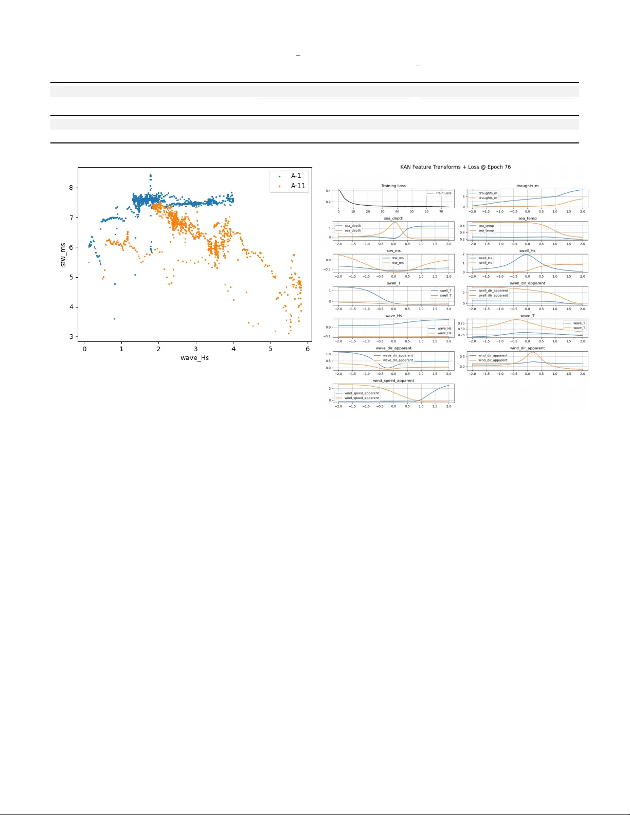
Physics-Informed Machine Learning for V essel Shaft Po wer and Fuel Consumption Prediction: Interpretable KAN-based Approach Hamza Haruna Mohammed Simula Resear ch Laboratory Oslo, Norway hamzahm@simula.no Dusica Marijan Simula Resear ch Laboratory Oslo, Norway dusica@simula.no Arnbjørn Maressa Navtor AS Egersund, Norway arnbjorn.maressa@navtor .com ©2025 IEEE. Personal use of this material is permitted. Permission from IEEE must be obtained for all other uses, in any current or future media, including reprinting/republishing this material for advertising or promotional purposes, creating new collectiv e works, for resale or redistribution to servers or lists, or reuse of any copyrighted component of this work in other works. Abstract —Accurate prediction of shaft rotational speed, shaft power , and fuel consumption is crucial for enhancing operational efficiency and sustainability in maritime transportation. Con ven- tional physics-based models provide interpr etability but struggle with real-w orld variability , while purely data-driven approaches achieve accuracy at the expense of physical plausibility . This paper introduces a Physics-Informed Kolmogorov–Ar nold Net- work (PI-KAN), a hybrid method that integrates interpretable univariate feature transformations with a physics-informed loss function and a leakage-free chained prediction pipeline. Using operational and en vironmental data from fi ve cargo vessels, PI-KAN consistently outperforms the traditional polynomial method and neural network baselines. The model achiev es the lowest mean absolute error (MAE) and r oot mean squared error (RMSE), and the highest coefficient of determination (R²) for shaft power and fuel consumption across all vessels, while maintaining physically consistent behavior . Interpretability analysis reveals r ediscovery of domain-consistent dependencies, such as cubic-like speed–power r elationships and cosine-like wav e and wind effects. These results demonstrate that PI-KAN achie ves both predictiv e accuracy and interpr etability , offering a robust tool for vessel performance monitoring and decision support in operational settings. Index T erms —kolmogor ov–arnold networks (KAN), physics- informed machine lear ning, hybrid models, interpretable ma- chine learning, fuel consumption modeling, shaft power predic- tion, maritime propulsion systems I . I N T RO D U C T I O N Accurate prediction of shaft RPM, shaft power , and fuel consumption is critical for optimizing the operational effi- ciency of maritime vessels. T raditional approaches rely on either physics-based model derived from propeller theory and engine thermodynamics [1], or purely data-driv en methods such as neural networks [2]. While Physics-based models provide interpretability and adherence to fundamental princi- ples, they often struggle to capture the complex, real-w orld variability observed in vessel operations. Con versely , data- driv en models excel at learning patterns from historical data but may produce physically implausible predictions due to their black-box nature [3]. Recent hybrid methods attempt to bridge this gap by combining physical knowledge with machine learning. Some approaches integrate physical equations as constraints within neural networks [4], while others employ linear combinations of physics-based and data-driv en components [3]. Ho wev er, these methods often struggle to balance the influence of physical la ws with empirical data, leading to either overly rigid or unconstrained predictions. Moreover , interpretability , a key requirement for maritime engineers remains limited in many deep learning-based solutions [5]. W e propose Physics-informed Kolmogoro v-Arnold Net- works (PI-KAN), a novel hybrid method that addresses these limitations through three key inno vations. First, it employs per- feature uni variate transformations followed by a linear com- bination, enabling flexible yet interpretable modeling. Unlike con ventional neural networks [6], PI-KAN decomposes the prediction task into simpler, e xplainable components while retaining the capacity to learn nonlinear relationships. Second, a physics-informed loss function dynamically balances data fidelity with physical consistency using an auto-tuned param- eter γ . This ensures that predictions adhere to fundamental propulsion principles without sacrificing accuracy . Third, the method incorporates a chained training pipeline with out- of-fold stacking to prev ent target leakage across sequential predictions (RPM → power → fuel consumption). V essel- wide tuning of γ further enhances generalization across div erse vessel types. The primary contributions of this work are: • Interpr etable Hybrid Ar chitecture : PI-KAN combines univ ariate feature transformations with linear combinations, offering transparency in how input features influence predictions. This directly addresses the interpretability requirements in maritime applications (Sections III-E and II-D), distinguishing it from opaque black-box deep learning models. • Adaptive Physics Data Balancing : The auto-tuned γ parameter ensures that physical constraints are neither ov erbearing nor negligible, adapting to the predictiv e uncertainty of each vessel. This mechanism outperforms fixed-weight physics-informed models by reducing bias in adverse conditions and maintaining accuracy across vessels. • Leakage-Free Sequential Prediction : The chained pipeline with out-of-fold stacking prev ents information leakage, enabling robust multi-tar get modeling. Compared to conv entional multi-task neural networks, this approach yields lower error propagation between shaft rpm, power , and fuel consumption, improving vessel-wide generalisation. The remainder of this paper is organized as follows: Section II revie ws related work in vessel performance modeling and hybrid approaches. Section III introduces the K olmogorov- Arnold Network (KAN) framework and its adaptation for maritime systems. Section IV details the PI-KAN architecture, physics-informed loss function, and training pipeline. Simi- larly , the same Section IV describes the e xperimental setup and datasets in subsection V -C. Section VI presents comparative results, and Section VII discusses vessel-wide generalization and future directions. I I . R E L A T E D W O R K V essel performance modeling has undergone significant ev olution in recent years, driv en by the growing a vailability of sensor data and the increasing demand for energy-ef ficient operations. Existing approaches can be broadly cate gorized into physics-based models, data-dri ven methods, and hybrid techniques that integrate both paradigms. A. Physics-Based Modeling T raditional physics-based approaches rely on first-principles equations deriv ed from propeller hydrodynamics and engine thermodynamics. These models, such as those based on propeller cube law and torque-speed relationships, provide interpretable predictions but often struggle with real-world variability due to simplifications in their formulations [7]. For instance, the influence of hull fouling or weather conditions is typically approximated using empirical correction factors, which may not generalize across different vessel types or operational conditions. Recent adv ancements have sought to refine these models by incorporating high-fidelity computational fluid dynamics (CFD) simulations [8]. While such methods improve accuracy , they remain computationally expensi ve and impractical for real-time vessel-scale predictions. B. Data-Driven Appr oaches Machine learning techniques have gained traction for their ability to capture complex patterns from historical operational data. Methods like random forests and gradient boosting hav e been applied to predict fuel consumption and shaft po wer [9]. Deep learning models, particularly recurrent neural networks (RNNs), hav e also been explored for time-series forecasting of vessel performance metrics [10]. Howe ver , purely data-driven models often lack interpretabil- ity and may produce physically implausible predictions when extrapolating beyond training conditions. For example, a neu- ral network might predict decreasing fuel consumption with increasing speed, a violation of basic propulsion principles [11]. C. Hybrid Methods T o address these limitations, hybrid methods have emerged as a promising direction. Physics-informed neural networks (PINNs) incorporate physical constraints directly into the loss function, ensuring predictions adhere to governing equations [4]. Another approach in volv es blending physics-based sub- models with data-driven corrections, as seen in [12], where a baseline physical model is augmented with a neural network to capture residual errors. Despite their advantages, existing hybrid methods face challenges in balancing the influence of physics and data. Fixed weighting schemes often lead to either overly rigid predictions or insufficient physical consistency . Moreov er, many approaches lack interpretability , making it difficult for maritime engineers to validate model behavior . D. Interpr etable and V essel-W ide Modeling Interpretability has become a key requirement for maritime applications, where engineers need to understand and trust model predictions. T echniques like SHAP (SHapley Additiv e exPlanations) hav e been applied to post-hoc explain black- box models [5]. Howe ver , these methods add computational ov erhead and may not fully rev eal the underlying decision logic. V essel-wide generalization is another significant challenge, as models must adapt to the di verse types of vessels and varying operating conditions. Some studies hav e explored transfer learning or meta-learning to improv e cross-vessel performance [13]. Ne vertheless, these methods often require extensi ve retraining or fail to maintain physical plausibility across the vessel. E. Comparison with Pr oposed Method The proposed PI-KAN method distinguishes itself from existing approaches in several key aspects. Unlike fixed hy- brid models, it dynamically balances physics and data via an auto-tuned loss-weighting parameter , ensuring adaptability across different operational regimes. The use of uni variate transformations and linear combinations provides inherent interpretability , allo wing engineers to inspect feature contri- butions directly . Furthermore, the chained prediction pipeline with out-of-fold stacking pre vents leakage while maintaining physical consistency . These innovations enable PI-KAN to achiev e superior accuracy and generalizability compared to con ventional physics-based, data-driven, or hybrid methods. I I I . B AC K G RO U N D O N K O L M O G O R OV – A R N O L D N E T W O R K S A N D V E S S E L P E R F O R M A N C E M O D E L L I N G T o establish the theoretical foundation for our proposed method, we first examine the mathematical framework of K olmogorov-Arnold Networks (KANs) and their relev ance Fig. 1: Architecture of the Physics-Informed K olmogorov–Arnold Network (PI-KAN) for v essel performance modeling. The model applies per-feature uni variate transformations followed by a linear combination layer , incorporates a physics-informed loss for propulsion consistency , and uses a leakage-free chained pipeline (RPM → shaft power → fuel consumption) with out-of-fold stacking to ensure physically plausible and robust multi-stage predictions as described in the Figure 2. to vessel performance modelling. The Kolmogoro v-Arnold representation theorem, a fundamental result in approximation theory , states that any multi variate continuous function can be expressed as a finite composition of uni variate functions and additions [14] [6]. This theoretical insight provides the basis for KAN architectures, which dif fer fundamentally from con ventional neural networks in their structural composition. A. Mathematical F oundations of KANs The Kolmogoro v-Arnold representation decomposes a mul- tiv ariate function f : [0 , 1] d → R into a sum of univ ariate functions: f ( x 1 , ..., x d ) = 2 d +1 X q =1 Φ q d X p =1 ϕ p,q ( x p ) ! (1) where ϕ p,q and Φ q are continuous univ ariate functions. This decomposition suggests that complex multi variate rela- tionships can be broken down into simpler, interpretable com- ponents, a property particularly v aluable for v essel systems, where physical interpretability is crucial. Unlike traditional multilayer perceptrons that apply nonlinear transformations to multiv ariate inputs, KANs implement this theorem by learning univ ariate functions along edges of a computational graph [15]. B. KANs vs. T raditional Neural Networks Three key differences distinguish KANs from conv entional neural network architectures. First, while standard networks use fixed activ ation functions (e.g., ReLU, sigmoid) applied to weighted sums of inputs, KANs learn adaptive univ ariate functions for each input feature. Second, the additi ve struc- ture of KANs naturally lends itself to interpretability , as the contribution of each component function can be examined independently . Third, the network width (i.e., the number of univ ariate functions) grows linearly with the input dimension, rather than exponentially , making KANs more parameter- efficient for high-dimensional problems. [16]. C. V essel P erformance Modelling Challenges V essel propulsion systems e xhibit complex nonlinear be- haviors that challenge traditional modelling approaches. The relationship between shaft rotational speed (RPM) and power output, for instance, follows a roughly cubic trend under ideal conditions, but actual measurements deviate due to factors like hull fouling, weather conditions, and engine wear [17]. These real-world complexities create a tension between physical first principles and data-driv en corrections - precisely the scenario where KANs’ hybrid nature offers adv antages. Physical models based on propeller theory typically express shaft power P as: P = 2 π nQ (2) where n is shaft speed and Q is torque. Howe ver , this idealized relationship overlooks the numerous environmental and operational factors that influence actual vessel perfor- mance. Data-driven approaches can capture these effects, but often lose connection to the underlying physics. The KAN framew ork provides a middle ground, where physical relation- ships can be encoded as priors while still allowing data-driven refinement of individual components. D. Historical Development of V essel P erformance Models The ev olution of vessel performance models has progressed through three distinct generations. First-generation models relied entirely on physical equations deri ved from nav al archi- tecture principles [18]. Second-generation models introduced empirical corrections to account for observed de viations from theory [19]. The current third generation combines these Fig. 2: Leakage-free chained prediction pipeline used in PI-KAN: shaft RPM is predicted first, followed by shaft power and then fuel consumption, with each stage receiving out-of-fold (OOF) predictions from the pre vious one to av oid target leakage and preserve physical causality . approaches through machine learning while attempting to preserve interpretability [20]. KANs represent a natural progression in this ev olution, as their structure aligns with the way maritime engineers traditionally decompose propulsion systems into subsystems (engine, propeller , hull) with well-characterized individual be- haviors. The network’ s additi ve structure mirrors the common practice of analyzing power losses separately for different components before combining them into a complete system model [21]. E. Interpr etability Requirements in Maritime Applications Unlike many machine learning applications where predic- tion accuracy alone suffices, maritime engineering demands models that pro vide actionable insights. Regulatory compli- ance, maintenance planning, and operational optimization all require understanding not just what the model predicts, b ut why [22]. KANs address this need through their transparent architecture, each uni variate function corresponds to a spe- cific input feature’ s transformation, and the final prediction combines these transformed inputs linearly . This interpretability proves particularly valuable when ana- lyzing anomalous vessel behavior . For instance, if a particular ship’ s fuel consumption deviates from vessel norms, engineers can examine the individual feature transformations to identify whether the discrepancy stems from engine performance, hull condition, or operational patterns [23]. Such diagnostic capa- bility remains challenging with conv entional neural networks, where feature interactions are complex and opaque. I V . M E T H O D O L O G Y : P H Y S I C S - I N F O R M E D K A N F O R V E S S E L F U E L A N D P OW E R P R E D I C T I O N The Physics-Informed KAN (PI-KAN) framew ork intro- duces a novel hybrid architecture that combines the in- terpretability of univ ariate feature transformations with the predictiv e power of physics-informed learning. The method addresses three critical challenges in maritime performance modeling: • maintaining physical plausibility while learning from data, • prev enting information leakage in sequential predictions, and • ensuring consistent performance across div erse vessel types. T ABLE I: Categorized input features used for shaft rpm, shaft po wer, and fuel consumption prediction. Category Featur e Description Operational V Speed through water (knots) T V essel draught (m), distance from waterline to keel En vironmental depth sea Sea depth below keel (m) t sea Sea surface temperature (°C) h wav e Significant wave height (m) T wav e W ave peak period (s) Swell h swell Swell height (m) T swell Swell period (s) d swell Swell direction relativ e to heading (°) d wav e W ave direction relative to heading (°) Wind v wind Apparent wind speed (m/s) d wind Apparent wind direction (° relative to vessel) Derived proxies V 3 Propeller cube-law proxy (cubed vessel speed) cos( d wav e ) Directional proxy for wave inci- dence Stacked (model outputs) P rpm Predicted shaft RPM → (input to power model) P shaf t power Predicted shaft power → (input to fuel model) Overall, the dataset provides a diverse and realistic foun- dation for ev aluating vessel performance-prediction methods across various operational conditions, vessel sizes, and main- tenance states. Figure 1 and Figure 2 illustrate the general framew ork of the proposed two-stage prediction approach. A. Ar chitectur e of PI-KAN for V essel P erformance Modeling The core of PI-KAN consists of per-feature univ ariate transformations implemented as small multilayer perceptrons (MLPs), followed by a linear combination layer . For an input feature vector x = [ x 1 , ..., x d ] , each feature x p undergoes a nonlinear transformation through a dedicated MLP ϕ p : h p = ϕ p ( x p ) (3) Where ϕ p is a two-layer neural network with sigmoid activ ation functions. The transformed features h p are then combined linearly to produce the final prediction ˆ y : ˆ y = d X p =1 w p h p + b (4) Here, w p and b are learnable weights and bias, respectiv ely . This architecture ensures that each feature’ s contribution to the prediction remains interpretable, as the influence of x p on ˆ y is mediated solely through its corresponding transformation ϕ p . In v essel performance prediction, the input features typically include shaft RPM, vessel speed, draft, and en vironmental conditions (e.g., wind speed, wav e height). The output tar- gets are shaft power P and fuel consumption ˙ m f , predicted sequentially to maintain physical causality . B. Physics-Informed Modeling and Physics-Informed Loss Function The training objectiv e combines data fidelity with physical consistency: L = L data + λ L physics + L reg (5) where L data is the mean absolute error (MAE) between pre- dictions and observations, L physics enforces adherence to first principles, and L reg is an ElasticNet term to reduce overfitting. a) Physics loss via empirical r esistance.: W e compute the physically required shaft power P Physical using the empirical resistance model for calm-water , wind, and wav e resistance giv en by physics equations, and the power as follows: ‘ P Physical =  R Calm + R W ind + R W ave  V The physics term for the po wer head penalizes deviations from this EF-based power: L PWR = MAE  ˆ P , P Physical  . (6) For the fuel head, we enforce consistenc y with a thermal- efficienc y relation: L FUEL = MAE  ˙ ˆ m f , P / ( ηH )  , (7) where η is the (effecti ve) engine ef ficiency and H the fuel’ s lower heating value. In our implementation, the ov erall physics loss is L physics = L PWR + L FUEL . b) Optional cube-law prior with vessel-specific k .: As an auxiliary , we additionally penalize de viation from the propeller cube law , ˜ L cube = MAE  ˆ P , k n 3  , where n is shaft RPM and k is a vessel-specific constant reflecting propeller and driv etrain characteristics. In prac- tice, k is pre-calibrated per vessel from training data (e.g., k = arg min k MAE( P , kn 3 ) , or the robust statistic k = median( P /n 3 ) over valid segments). When used, we add this term with a small weight: L physics = L PWR + γ ˜ L cube + L FUEL ( γ ∈ [0 , 1] ). c) A uto-balancing of physics weight.: The balancing parameter λ is updated during training to keep L data and L physics on comparable scales: λ new = clip  λ prev exp  η ( L data − L physics )  , λ min , λ max  . (8) This prevents either term from dominating and adapts the strength of physics guidance to the current prediction uncer- tainty . C. Chained T raining with Out-of-F old Stacking T o predict shaft RPM, power , and fuel consumption sequen- tially without leakage, PI-KAN employs a chained pipeline with out-of-fold (OOF) stacking: 1. Shaft RPM Prediction : T rain f RPM on folds { 1 , ..., K − 1 } , predict on fold K . 2. Po wer Prediction : Use OOF RPM predictions as input to train f PWR on folds { 1 , ..., K − 1 } , predict on fold K . 3. Fuel Prediction : Use OOF po wer predictions as input to train f FUEL . This approach ensures that downstream models (e.g., fuel prediction) nev er see the true values of upstream targets (e.g., RPM) during training, mimicking real-world deployment where future observations are unav ailable. D. V essel-W ide Hyperparameter T uning The auto-balancing parameter λ is optimized across the entire vessel to ensure consistent physical adherence. For each vessel v in the vessel: 1. Split data into training/validation sets D train v , D val v . 2. T rain PI-KAN on D train v with candidate λ values. 3. Select λ that minimizes median MAE across all D val v . This vessel-wide tuning adapts the physics guidance to the collectiv e beha vior of v essels while pre venting overfitting to individual ships’ idiosyncrasies. E. Interpr etability Through Univariate Responses The per-feature transformations ϕ p provide direct insight into ho w input variables influence predictions. F or example, the learned function ϕ RPM typically exhibits a near-cubic. The relationship for shaft po wer prediction aligns with propeller theory . En vironmental features, such as wav e height, exhibit threshold effects that become significant only when they exceed certain magnitudes. These interpretable patterns allow maritime engineers to validate the model behavior against domain kno wledge and identify anomalous vessel performance. For instance, an un- expectedly steep ϕ draft might indicate hull fouling, while a nonlinear ϕ wind could reveal windage effects specific to certain ship types. The combination of these components, interpretable archi- tecture, adapti ve physics guidance, leakage-free training, and vessel-wide tuning, enables PI-KAN to achieve both high accuracy and physical plausibility . The method’ s modular design also facilitates the incorporation of additional physical constraints or domain-specific modifications as needed for particular applications. T ABLE II: Number of instances and data periods for each vessel in training and test sets, including dry docking dates. V essel T rain Set Instances T est Set Instances T rain Dates (Start → End) T est Dates (Start → End) Dry Docking Date A-6 12,758 21,930 2023-01-09 → 2024-01-15 2024-01-15 → 2025-09-01 14/12/2022 A-8 18,145 8,663 2020-04-18 → 2020-10-13 2020-10-18 → 2021-09-14 14/04/2022 A-10 20,608 91,664 2020-05-11 → 2022-03-27 2022-04-22 → 2025-03-29 23/05/2023 A-12 23,186 96,258 2020-09-21 → 2023-02-19 2023-02-22 → 2025-05-07 09/11/2023 A-13 22,970 70,077 2020-04-20 → 2021-11-20 2021-11-22 → 2025-05-02 14/08/2023 V . E X P E R I M E N TAL E V A L U A T I O N A. Compar ed Modeling Approac hes a) P olynomial Model.: The PM is modeled using a multiplicativ e function of univ ariate polynomials: PM ( u ) = n Y i =1 p i ( u i ) , where n is the number of features, u is the input vector , and p i is the polynomial function applied to the feature u i . Features are selected iterativ ely by examining correlation with residual error , resulting in four input features: speed through water ( V ), draught ( T ), apparent wind speed ( v wind ), and swell height ( h swell ). A third-order polynomial is used for each feature. This formulation is computationally lightweight and interpretable, performing competiti vely on shaft rpm, but it underfits more complex nonlinearities in shaft power and fuel consumption. b) Multilayer P erceptr on (MLP).: As a data-driven base- line, we implement an MLP model whose input matches the selected (and engineered) features, with two hidden layers (37, 28; ReLU) and a linear head. Training uses Adam ( l r = 10 ( − 2) ), a batch size of 8, and up to 200 epochs with early stopping. The objectiv e is MSE plus a regularization penalty ( α = 0 . 01 , l 1 r atio = 0 . 5 ). While flexible for nonlinear mappings, the MLP remains a black box with limited interpretability and sensitivity to hyperparameters/regularization. c) PI-KAN: Each KAN module applies per -feature uni- variate subnetworks (Linear–activ ation–LayerNorm stacks) concatenated and linearly combined, optimized with a physics- guided MAE loss that integrates elastic-net regularization ( α =10 − 2 , ρ =0 . 5) and a weighted physics term ( λ tuned or auto-balanced). W e train with Adam (lr 10 − 3 ), batch size of 32 , MAE loss, and early stopping (up to 150 epochs) using an 80/20 split. 1) T raining: Leakage-free learning is ensured by 5- fold out-of-fold stacking, producing predicted_rpm and predicted_shaft_power for sequential targets. A chained pipeline (RPM → power → fuel) feeds predictions downstream, and fleet-wide λ values are tuned by sweeping candidates and selecting the best median MAE across vessels (Figure 2). B. Experimental Evaluation T o ev aluate the effecti veness of PI-KAN, we consider the following research questions (RQs): • RQ1: Does PI-KAN improv e prediction accuracy and physical plausibility compared to Polynomial, MLP , and standard KAN baselines? • RQ2: Can PI-KAN generalize vessel-wide across ships with different operational and environmental conditions? • RQ3: How interpretable are the learned transformations, and do they align with maritime domain knowledge (e.g., cubic speed–power law , cosine directional ef fects)? W e design our e valuation to explicitly address these ques- tions. Subsequent subsections present the compared methods, datasets, and ev aluation metrics. C. Dataset W e use 15 min operational and environmental logs from five cargo vessels (A-6, A-8, A-10, A-12, A-13). T able II reports train/test spans, sample counts, and most recent dry-dock dates. Coverage is heterogeneous: A-10/A-12 exceed 110k samples over more than 5 years; A-6 is balanced; A-8/A-13 are shorter and useful for assessing vessel-wide generalization. Maintenance records include scheduled dry-docking and mid- cycle propeller polishing; days-since-drydock were not used as inputs but are analysed separately . Features for performance modeling include operational/hydrodynamic variables (speed through water , V , RPM, draught, T , sea depth, and sea temperature) and en vironmental forcings (wave/swell height and direction, wind speed and direction; wind direction is relativ e to heading). W av e and wind fields are sourced from the Copernicus Marine Service [24]. D. Evaluation Metrics T o assess the performance of the vessel performance pre- diction method, we employ four commonly used regression metrics: • Mean Absolute Error (MAE) : Measures the average ab- solute deviation between predicted values ˆ y i and ground truth y i , defined as: MAE = 1 n n X i =1 | y i − ˆ y i | where n is the number of data points. MAE provides a straightforward measure of prediction accuracy . • Root Mean Squar e Error (RMSE) : Similar to MAE but penalizes larger errors more hea vily by squaring the deviations before av eraging: RMSE = v u u t 1 n n X i =1 ( y i − ˆ y i ) 2 RMSE emphasizes the impact of significant outliers. • Mean Absolute Per centage Error (MAPE) : Expresses prediction error as a percentage relativ e to the true values: MAPE = 1 n n X i =1     y i − ˆ y i y i     × 100% providing an interpretable, scale-independent measure of accuracy . • Coefficient of Determination ( R 2 ) : Indicates the pro- portion of v ariance in the ground truth explained by the predictions: R 2 = 1 − P n i =1 ( y i − ˆ y i ) 2 P n i =1 ( y i − ¯ y ) 2 where ¯ y is the mean of the actual v alues. Higher R 2 values denote better model fit. V I . R E S U LT S A N D C O M PA R A T I V E A N A L Y S I S A. Results for RQ1 and RQ2: V essel-W ide P erformance Eval- uation Using the consolidated benchmark in T able III, the Physics- Informed KAN (PI-KAN) attains the strongest vessel-wide performance on the ener gy-related targets : it achieves the lowest MAE and RMSE for shaft power and fuel consumed across all five vessels (A-6, A-8, A-10, A-12, A-13), and simultaneously yields the highest R 2 in those targets for each vessel. In contrast, for shaft rpm the P olynomial baseline attains the lowest MAE/RMSE on 3/5 vessels (A-10, A-12, A- 13), with PI-KAN leading on A-8 and a little bit on A-6 vessel. Notably , PI-KAN still secures the top R 2 on shaft rpm for 3/5 vessels (A-6, A-8, A-10), indicating better explained variance ev en where absolute-error minima are held by Polynomial. These results align with expectations: po wer and fuel are tightly constrained by physics (e.g., propeller laws and energy balance), where physics guidance helps; rpm beha ves more linearly and is well captured by a low-bias polynomial regres- sor as illustrated in Figure 3, showing the speed versus target (rpm, shaft power , and fuel consumption) relationship. B. Results for RQ1: T ar get-Specific Analysis a) Shaft RPM.: Polynomial regression yields the smallest absolute errors across most vessels, suggesting that rpm dy- namics within the observed en velope are well approximated by low-order trends. Ho wever , PI-KAN often achiev es higher R 2 values (A-6, A-8, A-10), suggesting improv ed v ariance explanation and greater robustness to distributional shifts. (a) A-6 V essel: Shaft RPM vs speed (b) A-6 V essel: Shaft power vs speed (c) A-6 V essel: Fuel consumed vs speed Fig. 3: Comparison of actual vs predicted performance metrics for A-6 V essel. b) Shaft P ower .: PI-KAN consistently achiev es the low- est MAE/RMSE and the highest R 2 across all vessels, while preserving the expected cubic-like relationship between rpm and power . The physics-informed loss curbs implausible re- sponses in high-power regimes and stabilizes learning under sparse, extreme conditions. c) Fuel Consumption.: PI-KAN is uniformly best (lo west MAE/RMSE, highest R 2 ) across all vessels. Improvements are most pronounced on vessels and periods with stronger T ABLE III: Benchmark performance on the test set (relative errors, overall values) across different targets. MAE: Mean Absolute Error, RMSE: Root Mean Squared Error, R 2 : Coefficient of Determination. V essel Method shaft rpm shaft power fuel consumed MAE RMSE R 2 MAE RMSE R 2 MAE RMSE R 2 A-6 Polynomial 2.34 2.97 88.37 12.39 15.80 60.34 17.52 22.98 2.01 A-6 MLP 6.74 8.19 11.91 13.55 17.93 48.93 25.18 31.24 -81.04 KAN 10.42 11.61 77 33.52 40.47 61.51 26.01 25.25 71.42 PI-KAN 1.88 3.33 90.79 8.89 10.96 77.27 11.24 13.98 72.47 A-8 Polynomial 2.34 3.02 85.85 13.98 18.18 34.08 16.42 21.05 -7.89 A-8 MLP 2.64 3.36 82.52 9.76 12.10 70.80 17.14 21.48 -12.36 KAN 3.17 3.90 76.34 15.24 18.64 30.70 12.44 15.27 43.20 PI-KAN 1.91 2.78 86.61 7.60 9.49 71.64 9.31 11.27 66.09 A-10 Polynomial 2.51 3.76 12.69 21.29 23.42 -17 25.18 26.93 -39.7 A-10 MLP 12.20 14.96 -12.82 12.52 15.13 -11.34 70.80 78.71 -16.64 KAN 7.73 8.94 -39.4 28.14 31.70 -40.2 13.59 17.08 -63.3 PI-KAN 3.04 4.22 48.86 10.05 14.32 54.04 9.10 13.27 15.46 A-12 Polynomial 3.14 4.38 80.61 22.17 26.72 1.24 24.88 31.41 -20.62 A-12 MLP 9.52 10.64 -14.55 29.72 31.78 -39.64 12.17 15.91 -47.87 KAN 7.39 9.01 18.00 25.11 28.94 -15.88 16.29 20.42 31.15 PI-KAN 5.01 6.29 61.18 10.57 15.14 70.13 9.54 14.24 68.93 A-13 Polynomial 2.35 3.26 73.24 16.48 18.52 -13.55 25.58 28.66 -26.90 A-13 MLP 19.37 23.75 -13.23 53.62 61.11 -34.35 26.16 30.44 -11.15 KAN 15.02 17.08 -63.66 41.64 36.88 -47.43 32.81 38.42 -56.3 PI-KAN 5.22 5.93 54.16 10.33 12.88 57.16 15.60 18.16 16.00 en vironmental forcing (e.g., A-8, A-10), where physics con- straints regularize the mapping and reduce error propagation from upstream targets. C. Results for RQ2: Adversarial W eather Case Study Under adverse conditions (T able IV), PI–KAN yields MAPE of 22.63% (A–1) and 10.17% (A–11), with signed ME of +22.41% and +5.55%, respectiv ely . The traditional baseline shows signed ME of +12% (A–1) and − 8% (A–11), but MAPE was not computed, limiting direct comparison. Figure 4 shows that A–11 reduces speed as wa ves increase, whereas A–1 maintains a near-constant setpoint; the resulting variance in power/fuel explains the higher error on A–1. Overall, PI-KAN is robust in aggregate, but voyage-le vel bias can increase under heavy seas, motiv ating policy-aw are calibration for rough-weather operations. D. Results for RQ3: Interpretability Insights for (PI-)KAN Models T o assess interpretability , we visualize the learned univari- ate transformation functions (KAN splines) for each input feature (Figure 5). Unlike black-box neural networks, (PI- )KAN explicitly parameterizes and exposes feature-wise non- linear mappings, enabling v alidation of model behavior ag ainst nav al-architecture intuition. The learned transformations recover physically plausible structures: • Speed and power: The transformation for ship speed through water ( stw_ms ) exhibits a cubic-like trend, consistent with the well-known cubic relationship be- tween speed and resistance. Likewise, the rpm → po wer mapping is near-cubic with low-rpm de viations (engine T ABLE IV: Performance analysis of adversarial weather conditions (fuel consumption). T est voyage window = departure for a duration of travel in that period. (All other voyages (different voyage ids) go into training). T raditional model results are added for comparison. V essel Departure (UTC) Duration Samples PI-KAN T raditional ME% (signed) MAPE% ME% (signed) MAPE% A-1 2020-07-28 18:30:00 10 days 02:45 944 22.41 22.63 12.00 – A-11 2020-11-29 03:15:00 13 days 05:30 179 5.55 10.17 -8.00 – Fig. 4: Adversarial weather response (A–1 vs. A–11): vessel speed as a function of wa ve height. A–11 reduces speed at higher waves, while A–1 holds a near-constant setpoint. This difference aligns with T able IV: lower error on A–11 (ME=+5.55%, MAPE=10.17%) versus higher error on A–1 (ME=+22.41%, MAPE=22.63%). inefficienc y) and mild high-rpm flattening (propeller ven- tilation/limits). • Dir ectional effects: Apparent wave_dir_apparent and wind_dir_apparent sho w cosine-like patterns, capturing alignment between heading and en vironmental forcing (head vs. following seas/winds). • Sea state and bathymetry: swell_Hs and sea_depth display nonlinear peaks, highlighting regimes where hy- drodynamic and added resistance grow more influential; wa ve-height effects are monotone beyond operationally relev ant thresholds. • Draft–power coupling: The draft transformation yields a shallow U-shaped relation with an identifiable optimum, aligning with expected resistance–displacement trade- offs. T raining curves indicate stable conv ergence after ∼ 60 epochs. T aken together, these mappings explain why PI- KAN achieves the strongest accuracy on energy-related targets (shaft power , fuel): gains arise from physically consistent behaviors rather than spurious correlations. In practice, the exposed splines provide actionable diagnostics (sanity checks for re gime validity , early detection of sensor bias) and facilitate communication with operators through interpretable, physics- aligned responses. Fig. 5: Learned univ ariate feature transformation functions of the KAN model for shaft power prediction (epoch 76). Each subplot shows how an input feature is nonlinearly mapped before combination in the network. The transformations reflect physically meaningful patterns, including cubic-like dependence on ship speed through water ( stw_ms ), cosine-like wind and wav e directional effects, and localized nonlinear responses to swell and sea depth. The top-left subplot displays the training loss curve con verging after ∼ 60 epochs. V I I . D I S C U S S I O N A N D C O N C L U S I O N PI–KAN advances vessel performance modelling by bridg- ing physical laws and machine learning. It improv es predictiv e accuracy , physical plausibility , and interpretability while offer - ing insights into operational policies under challenging condi- tions. PI–KAN consistently outperforms traditional baselines on shaft power and fuel across all vessels, while Polynomial regression remains competiti ve for shaft rpm . Under rough weather , operational policy governs prediction error: adapti ve slowdo wn reduces power/fuel variance and bias, whereas constant-speed strategies amplify error . a) Limitations.: Despite strong vessel-wide performance, PI-KAN has limitations: (1) its additive, univ ariate design under-represents higher -order interactions (e.g., draft–trim–sea state coupling); (2) physics-regularization introduces hyperpa- rameter sensitivity , and embedded laws assume quasi-steady conditions [25]; (3) training costs are higher than classical baselines, complicating on-board deployment without pruning or distillation [26]; and (4) KAN remains an ev olving archi- tecture [27], requiring further research for industrial adoption. b) Challenges in V essel-W ide Generalisation.: Model robustness is affected by domain shifts between vo yages (loading, fouling, weather), class imbalance in rare adv erse conditions, and sensor biases [28]. Global physical constants may not fully capture vessel-specific de viations, and opera- tional policies (e.g., maintaining a constant speed under high seas) interact with sea state to amplify variance and bias. c) Futur e Dir ections.: Future work will pursue selec- tive interactions to capture sparse multiv ariate ef fects while preserving interpretability [29]; uncertainty quantification via Bayesian PI–KAN for calibrated predicti ve interv als; continual calibration to adapt online to drift and regime shifts [30]; hybrid modeling that couples Polynomial (rpm) with PI–KAN (power/fuel) and emplo ys model compression for edge deploy- ment; and policy-awar e bias correction using voyage-specific bias heads to mitigate control-induced extremes. D A TA A N D C O D E A V A I L A B I L I T Y The datasets and source code underlying this study are subject to contractual confidentiality and data-sharing restric- tions with the industrial partner and therefore cannot be made publicly av ailable. A C K N O W L E D G M E N T This work was supported by the Research Council of Norway through the GASS project (Grant No. 346603) and the eX3 infrastructure (Contract No. 270053). W e used data from the E.U. Copernicus Marine Service Information 1 2 3 4 The authors thank Joachim Haga, Glenn T erje Lines, Do- gan Altan, Akriti Sharma, and T etyana Kholodna for their contributions to the empirical resistance formulas and the modeling formulation, as well as for v aluable discussions on the methodology . R E F E R E N C E S [1] S. Saettone, S. T avakoli, B. T askar , M. Jensen et al. , “The importance of the engine-propeller model accuracy on the performance prediction of a marine propulsion system in the presence of wa ves, ” Applied Ocean Resear ch , 2020. [2] N. Assani, P . Mati ´ c, N. Ka ˇ stelan, and I. ˇ Cavka, “ A review of artificial neural networks applications in maritime industry , ” IEEE access , 2023. [3] L. Liao and F . K ¨ ottig, “ A hybrid frame work combining data-driv en and model-based methods for system remaining useful life prediction, ” Applied Soft Computing , 2016. [4] O. Bourchas and G. Papalambrou, “Physics informed neural networks for vessel main engine power prediction, ” Ocean Engineering , 2025. [5] S. Zikas, K. Gkirtzou, I. Filippopoulos, D. Kalatzis et al. , “Explainable ai models for iot-based shaft po wer prediction and comprehensive performance monitoring, ” Electr onics , 2025. [6] Z. Liu, Y . W ang, S. V aidya, F . Ruehle, J. Halverson, M. Solja ˇ ci ´ c, T . Y . Hou, and M. T egmark, “Kan: Kolmogorov-arnold networks, ” arXiv pr eprint arXiv:2404.19756 , 2024. [7] P . Karagiannidis, “Data-driven ship propulsion modelling with appli- cations in the performance analysis and fuel consumption prediction, ” dspace.lib .ntua.gr, T ech. Rep., 2019. 1 https://doi.org/10.48670/moi- 00016 2 https://doi.org/10.48670/moi- 00017 3 https://doi.org/10.48670/moi- 00021 4 https://doi.org/10.48670/moi- 00022 [8] K. Kan, Y . Zheng, H. Chen, D. Zhou, J. Dai, M. Binama et al. , “Numerical simulation of transient flow in a shaft extension tubular pump unit during runaway process caused by po wer failure, ” Renewable Ener gy , 2020. [9] and S Krishnappa, S. Kamangar , R. Baig, T . Khan et al. , “Machine learning prediction and optimization of performance and emissions characteristics of ic engine, ” Sustainability , 2023. [10] M. Abebe, Y . Shin, Y . Noh, S. Lee, and I. Lee, “Machine learning approaches for ship speed prediction towards energy efficient shipping, ” Applied Sciences , 2020. [11] P . Karagiannidis and N. Themelis, “Data-driven modelling of ship propulsion and the effect of data pre-processing on the prediction of ship fuel consumption and speed loss, ” Ocean Engineering , 2021. [12] Q. Liang, P . Han, E. V anem et al. , “ A hybrid approach integrating physics-based models and expert-augmented neural networks for ship fuel consumption prediction, ” Journal of Offshore Mechanics and Ar ctic Engineering , 2025. [13] A. Kalafatelis, N. Nomik os, A. Giannopoulos et al. , “ A surve y on predictiv e maintenance in the maritime industry using machine and federated learning, ” No complete venue information available , 2024. [14] X. Liu, “Kolmogoro v superposition theorem and its applications, ” core.ac.uk, T ech. Rep., 2015. [15] K. Hornik, “ Approximation capabilities of multilayer feedforward net- works, ” Neural networks , 1991. [16] S. Qian, H. Liu, C. Liu, S. W u, and H. S. W ong, “ Adaptiv e activ ation functions in conv olutional neural networks, ” Neur ocomputing , 2018. [17] M. T erziev , T . T ezdogan, and A. Incecik, “Scale effects and full-scale ship hydrodynamics: A revie w , ” Ocean Engineering , 2022. [18] J. Falzarano, “Ship resistance and propulsion: practical estimation of ship propulsive power , ” arc.aiaa.org, T ech. Rep., 2018. [19] J. Holtrop, “ A statistical analysis of performance test results, ” Interna- tional Shipbuilding Pr ogress , 1977. [20] X. Lang, D. W u, and W . Mao, “Comparison of supervised machine learning methods to predict ship propulsion po wer at sea, ” Ocean Engineering , 2022. [21] B. Naujoks, M. Steden, S. Muller et al. , “Evolutionary optimization of ship propulsion systems, ” 2007 IEEE Congress on Evolutionary Computation , 2007. [22] M. Abuella, M. Atoui, S. No waczyk, S. Johansson et al. , “Data- driv en explainable artificial intelligence for energy efficienc y in short-sea shipping, ” Unable to determine the complete publication venue , 2023. [23] A. Coraddu, L. Oneto, A. Ghio, S. Savio et al. , “Machine learning ap- proaches for impro ving condition-based maintenance of na val propulsion plants, ” Unable to determine the complete publication venue , 2016. [24] Copernicus, “Copernicus: Earth observ ation component of the european union’ s space programme, ” https://www .copernicus.eu/en, Jul. 2025, accessed: 2025-09-28. [25] B. T askar, K. Y um, S. Steen, and E. Pedersen, “The effect of waves on engine-propeller dynamics and propulsion performance of ships, ” Ocean Engineering , 2016. [26] A. Algarni, T . Acarer, and Z. Ahmad, “ An edge computing-based prev entive framew ork with machine learning-integration for anomaly detection and risk management in maritime wireless communications, ” IEEE Access , 2024. [27] S. A. Faroughi, F . Mostajeran, A. H. Mashhadzadeh, and S. Faroughi, “Scientific machine learning with kolmogorov-arnold networks, ” arXiv pr eprint arXiv:2507.22959 , 2025. [28] I. Durlik, T . Miller , D. Cembro wska-Lech, A. Krzemi ´ nska et al. , “Navigating the sea of data: a comprehensiv e review on data analysis in maritime iot applications, ” Applied Sciences , 2023. [29] Y . Cai, L. Li, Y . W ang, and G. Li, “ An efficient and interpretable autoregressi ve model for high-dimensional tensor-v alued time series, ” arXiv preprint arXiv:2506.01658, T ech. Rep., 2025. [30] P . Zhang, Z. Gao, L. Cao, F . Dong, Y . Zou, K. W ang et al. , “Marine systems and equipment prognostics and health management: a system- atic revie w from health condition monitoring to maintenance strategy , ” Machines , 2022.