Stochastic Optimal Control with Side Information and Bayesian Learning

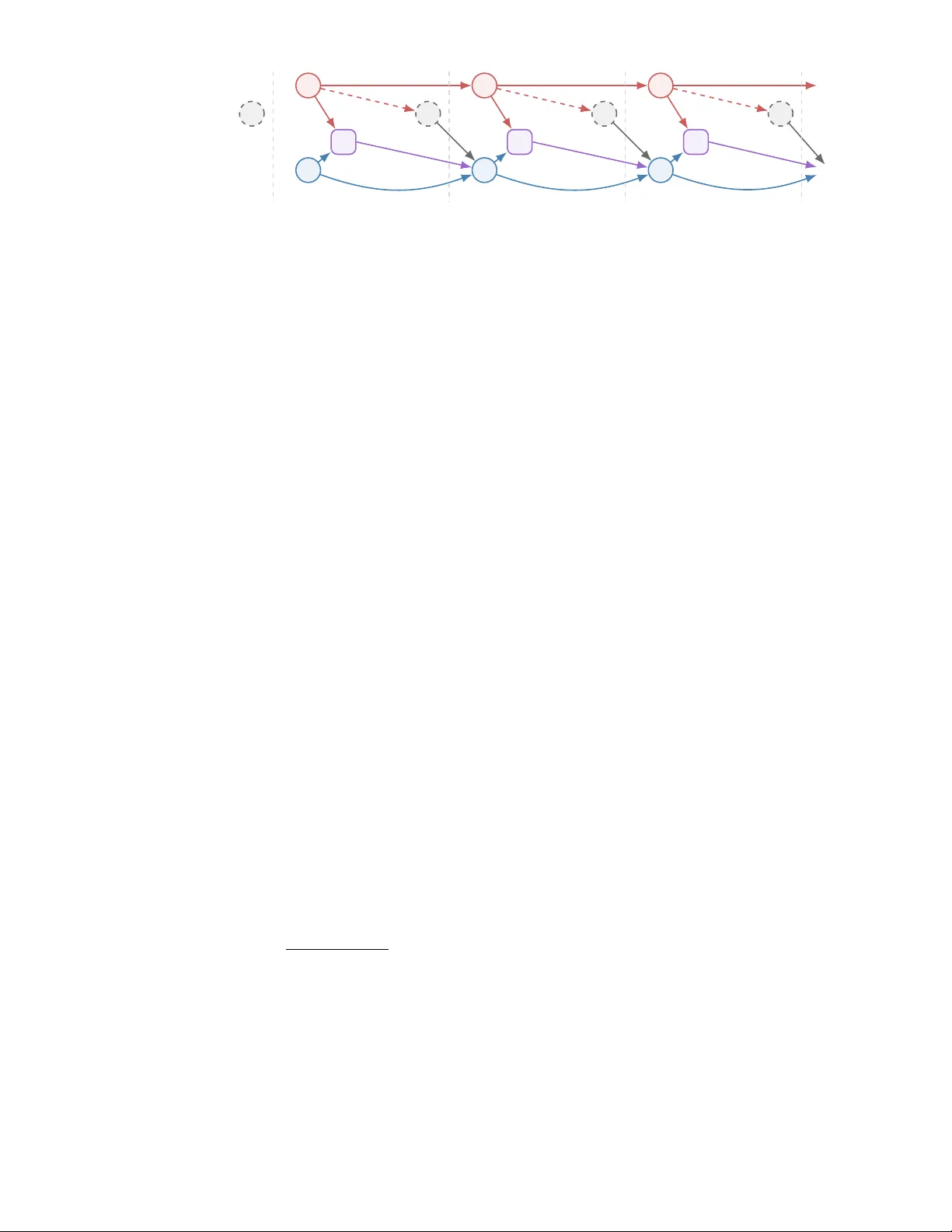
Sto c hastic Optimal Con trol with Side Information and Ba y esian Learning Johannes Milz ∗ Alexander Shapiro † Enlu Zhou ‡ F ebruary 26, 2026 Abstract W e study infinite-horizon sto c hastic optimal con trol problems with observ able side information: a Mark o v c hain that modulates an unkno wn con text-conditional randomness distribution. Since this distribution is unkno wn, we propose a Bay esian reformulation based on a parametric densit y mo del and posterior predictive dynamics, which yields a Bay esian Bellman equation. W e prov e p osterior consistency under Marko v samples and, under correct sp ecification and identifiabilit y , uniform con- v ergence of the Bay esian v alue function. Finally , we establish Bernstein–von Mises-t yp e asymptotic normalit y for the data-driv en contextual optimal v alue. 1 In tro duction Con textual optimization addresses decision making under uncertain ty with side information (also kno wn as con text or cov ariate) av ailable at the time of decision. In its static (one-stage) form, the decision mak er observes a context and then c ho oses an action that optimizes the conditional exp ected p erformance. T o learn the optimal decision rule that maps from an observ ed context to the optimal ac- tion, there are sev eral differen t paradigms, including decision rule optimization, sequen tial learning and optimization, and in tegrated learning and optimization (see the recent paper [ 18 ] for a comprehensiv e surv ey). Con textual optimization has also b een studied in multi-stage settings where a state evolv es o ver time under a policy and the context ma y shap e rew ards and transition kernels from stage to stage. Several existing mo dels instantiate dynamic con textual optimization. In the contextual multi-armed bandit, the learner rep eatedly observes a context and selects an arm, receiving bandit feedback while seeking lo w regret (see, e.g., [ 13 ]). In contextual Marko v decision pro cesses (CMDPs), an episo de is gov erned b y an observ ed, typically static con text that parameterizes b oth transitions and rewards; founda- tional work established this mo del and studied planning/learning guaran tees, while subsequent results pro vided regret and sample-complexit y bounds under realizability assumptions and oracle-based regres- sion [ 7 , 12 , 14 ]. When the con text ev olves within an episo de, Dynamic Contextual MDPs (DCMDPs) allo w history-dependent or time-v arying contexts and analyze algorithm’s regret under additional structure (e.g., logistic DCMDPs) [ 25 ]. A closely related line of research mo dels the con text as a finite-state Marko v chain (often called a regime or mode), yielding Mark ov-jump/Mark ov-switc hing ∗ Georgia Institute of T ec hnology , Atlan ta, Georgia 30332, USA ( johannes.milz@isye.gatech.edu ). The research of this author was partially supp orted b y the National Science F oundation under Award No. DMS-2410944. † Georgia Institute of T echnology , A tlanta, Georgia 30332, USA ( ashapiro@isye.gatech.edu ). The research of this author w as partially supp orted b y Air F orce Office of Scien tific Researc h (AF OSR) under Gran t F A9550-25-1-0310. ‡ Georgia Institute of T ec hnology , Atlan ta, Georgia 30332, USA ( enlu.zhou@isye.gatech.edu ). The researc h of this author was partially supp orted b y Air F orce Office of Scien tific Researc h (AFOSR) under Grant F A9550-25-1-0310 and the National Science F oundation under Aw ard ECCS-2419562. 1 systems (MJLS) in which mo de-dep endent dynamics are con trolled via dynamic programming or cou- pled Riccati equations; classical treatments typically assume the mo de transition matrix and noise statistics are known rather than learned from data (see, e.g., [ 6 , 9 , 11 ]). A related stream studies m ulti- p erio d in ven tory control under Mark ov-modulated demand, with kno wn demand distribution driven b y a Marko v chain [ 1 , 4 , 5 , 8 , 16 , 19 , 24 ]. In this paper, we in tro duce a contextual stochastic optimal con trol problem, in which (i) the con text is observ able and evolv es according to a Marko v chain, and (ii) the distribution of the exogenous randomness, conditional on the context, is unkno wn and must b e learned from sequen tial data. T o estimate this conditional distribution, we p osit a regression mo del and learn its parameters with a Ba y esian approach, then solv e a Bay esian av erage estimate of the original control problem. Compared to CMDPs and DCMDPs, our form ulation departs by imp osing Mark ovian con text dynamics (rather than p er-episo de static or history-dep endent con text) and our approac h hinges on Ba y esian learning of the conditional distribution. Unlik e classical MJLS, whic h presumes kno wn context transition probabilities and randomness distributions, we learn the context-conditional randomness distribution from data and integrate Bay esian learning into decision making. Conceptually , our approach can b e view ed as extending the episo dic Bay esian optimal con trol in [ 23 ] to a Marko vian contextual setting. W e summarize our contributions as follo ws: • W e in tro duce a new model for sto chastic optimal con trol with side information (observ ed con text) and unknown randomness distribution. It pro vides a modeling framework for a wide range of application problems. F or example, it can address p ortfolio optimization with side information suc h as time-v arying economy factors. • W e prop ose a reformulation of the original problem by incorporating Bay esian learning of the con text-conditional randomness distribution. The Bay esian learning approach sequen tially up- dates the p osterior distribution with observ ed con text-randomness data, and the Ba yesian av erage estimate of the cost function serves a surrogate of the original (unknown) ob jective. • W e theoretically show that the optimal v alue functions of the reformulated problem conv erge uniformly to the true v alue function as the data size increases. W e also develop a Bernstein–von Mises-t yp e asymptotic normality result for the data-driven contextual optimal v alue. 2 Problem Statemen t W e consider the (discrete time, infinite horizon) Sto chastic Optimal Control (SOC) mo del: min π ∈ Π E π  P ∞ t =1 γ t − 1 c ( x t , u t , ξ t )  , (1) where γ ∈ (0 , 1) is the discoun t factor and Π is the set of p olicies given b y Π = n π = ( π 1 , π 2 , . . . ) : u t = π t ( x t , η [ t ] , ξ [ t − 1] ) , u t ∈ U , x t +1 = F ( x t , u t , ξ t ) , t = 1 , 2 , . . . o . (2) Here v ariables x t ∈ R n , t = 1 , 2 , . . . , represent the state of the system with state space X ⊂ R n , u t ∈ R m , t = 1 , 2 , . . . , are con trols, ξ t ∈ Ξ, t = 1 , 2 , . . . , are random v ectors, and η t ∈ H , t = 1 , 2 , . . . , are observ able context v ariables taking v alues in a finite set H . The set Ξ is a closed subset of R d , the one-stage cost function c : R n × R m × R d → R is measurable, and F : R n × R m × R d → R n is a measurable mapping. The control set U is a nonempt y subset of R m . W e assume that the v alues x 1 , ξ 0 , and η 1 are deterministic, and that the cost function c : X × U × Ξ → R is b ounded. Moreo v er, we assume that the probabilit y la w of the random pro cess { ( ξ t , η t ) } t ≥ 1 do es not dep end on the decisions. The optimization in ( 1 ) is p erformed o ver p olicies π ∈ Π determined by decisions u t and state v ariables x t , which are functions of the context histories η [ t ] : = ( η 1 , . . . , η t ) and randomness histories ξ [ t − 1] : = ( ξ 0 , . . . , ξ t − 1 ) and satisfy the feasibility constrain ts ( 2 ). W e consider the data-driven scenario that a decision maker does not hav e access to the distribution of ξ conditional on the context η but can observe data { ( ξ i , η i ) , i = 1 , . . . , N } . 2 ξ 0 η 1 x 1 u 1 u 1 = π ( x 1 , η 1 ) ξ 1 η 2 x 2 x 2 = F ( x 1 , u 1 , ξ 1 ) u 2 u 2 = π ( x 2 , η 2 ) ξ 2 η 3 x 3 x 3 = F ( x 2 , u 2 , ξ 2 ) u 3 u 3 = π ( x 3 , η 3 ) ξ 3 . . . . . . . . . . . . ϖ η 1 ,η 2 ϖ η 2 ,η 3 ϖ η 3 ,... q ( ·| η 1 ) q ( ·| η 2 ) q ( ·| η 3 ) Context Randomness Decision State t = 0 t = 1 t = 2 t = 3 . . . Figure 1: Timeline of the data (context and randomness) pro cess, system dynamics, and con trol pro cesses. The context η t ev olv es according to the transition probabilit y ϖ η t ,η t +1 , and generates the randomness ξ t via q ( ·| η t ). The action u t = π ( x t , η t ) is chosen based on state and context, driving the system dynamics x t +1 = F ( x t , u t , ξ t ). Mark ovian con textual dynamics and p olicy simplification. W e assume that { η t } t ≥ 1 is a time-homogeneous Marko v chain on a finite state space H with transition probabilities ϖ h,h ′ : = P ( η t +1 = h ′ | η t = h ) , h, h ′ ∈ H . (3) Moreo v er, conditional on η t , the random vector ξ t has densit y q ( ·| η t ) and is conditionally independent of the past. In addition, η t +1 conditional on η t is independent of ξ [ t ] . Consequently , the augmented state z t : = ( x t , η t ) defines a controlled Mark ov pro cess, and ( 1 ) can b e view ed as an infinite-horizon MDP with state z t and action u t . In general, an admissible p olicy ma y dep end on the en tire observed history , that is, u t = π t ( x t , η [ t ] , ξ [ t − 1] ). Under the ab ov e Marko vian assumptions, ( x t , η t ) is a sufficient state, and hence there is no loss of op- timalit y in restricting atten tion to policies of the form u t = π t ( x t , η t , ξ [ t − 1] ). Moreov er, since ξ t is con- ditionally independent of the past given η t , one can further restrict to Marko v p olicies u t = π t ( x t , η t ), whic h is the policy class used throughout the paper. W e illustrate the problem form ulation in Figure 1 . Restricting to the Mark ov p olicies, the Bellman equation of ( 1 ) is V ∗ ( x, η ) = inf u ∈U E ξ ∼ q ( ·| η ) h c ( x, u, ξ ) + γ E η ′ | η  V ∗ ( F ( x, u, ξ ) , η ′ )  i , (4) where η ′ denotes the next con text state with distribution P ( η ′ = ¯ η | η ) = ϖ η , ¯ η . Under the sp ecified assumptions, the asso ciated Bellman op erator is a γ -contraction under the uniform norm on b ounded functions on X × H , and hence ( 4 ) admits a unique b ounded solution V ∗ , which is the optimal v alue function of ( 1 ). Ba yesian reform ulation. Since the conditional density q ( ξ | η ) is unknown, the Bellman equation ( 4 ) is not av ailable and needs to b e estimated. T o this end, we take a Bay esian approach. Supp ose that the conditional densit y q ( ξ | η ) is mo deled by a parametric density family { f ( ξ | η , θ ) : θ ∈ Θ } with unkno wn parameter θ , where Θ ⊂ R d . Let p ( θ ) b e a prior density on Θ. W e observe data η 1 , . . . , η N ∈ H and ξ 1 , . . . , ξ N , where ξ i is generated according to the conditional densit y q ( ·| η i ) and is conditionally indep endent of ξ [ i − 1] giv en { η i } N i =1 . Moreov er, η 1 is deterministic. Giv en data ( ξ i , η i ), i = 1 , . . . , N , the p osterior density is p N ( θ ) = f N ( θ ) p ( θ ) R Θ f N ( θ ) p ( θ ) d θ , where f N ( θ ) : = f ( ξ 1 | η 1 , θ ) N Y i =2 f ( ξ i | η i , θ ) ϖ η i − 1 ,η i . (5) F or a b ounded random v ariable Y on Ξ, we define its p osterior predictive conditional exp ectation by E p N | η [ Y ] : = E θ ∼ p N h E ξ ∼ f ( ·| η ,θ ) [ Y ] i = Z Θ Z Ξ Y ( ξ ) f ( ξ | η , θ ) p N ( θ ) d ξ d θ. (6) 3 Data { ( ξ i , η i ) } N i =1 Posterior p N in ( 5 ) Bay esian value function V ∗ N in ( 7 ) Bay esian policy π ∗ N in ( 8 ) Figure 2: Schematic of the Ba yesian learni ng and con trol pipeline giv en a dataset of size N . The accum ulated historical data { ( ξ i , η i ) } N i =1 is used to construct the p osterior p N , which defines the predictiv e exp ectation required to solve for the Bay esian v alue function V ∗ N and the corresp onding optimal policy π ∗ N . This pro cess is rep eated as new data is obtained. The corresponding Bay esian v alue function V ∗ N on X × H is defined as the optimal v alue that satisfies the Bay esian Bellman equation V ∗ N ( x, η ) = inf u ∈U E p N | η h c ( x, u, ξ ) + γ E η ′ | η  V ∗ N ( F ( x, u, ξ ) , η ′ )  i . (7) By the same contraction argument as abov e, for eac h N ∈ N , ( 7 ) admits a unique b ounded solution V ∗ N . A Ba y esian optimal (stationary Mark ov) p olicy is given by a measurable selector π ∗ N ( x, η ) ∈ arg min u ∈U E p N | η h c ( x, u, ξ ) + γ E η ′ | η  V ∗ N ( F ( x, u, ξ ) , η ′ )  i . (8) W e illustrate this scheme in Figure 2 . Remark 1. The Bay esian Bellman equation ( 7 ) can b e view ed as a Bay esian av erage appro ximation of the original Bellman equation ( 4 ). It is also p ossible to replace the exp ectation E θ ∼ p N with a risk measure with respect to the pos terior, leading to a Bay esian risk form ulation inspired b y [ 15 , 27 ]. The risk measure (including exp ectation) represen ts the decision maker’s risk attitude to wards the epistemic uncertain t y brought b y the unknown con text-conditional distribution of the randomness. Remark 2. It is imp ortan t to distinguish the role of the randomness ξ in the learning versus the con trol phase. The p osterior density p N is constructed using the historical dataset { ( ξ i , η i ) } N i =1 . In con trast, the v ariable ξ app earing in the expectations ( 6 ) and ( 7 ) represen ts a generic future uncertain randomness. While the con trol must b e chosen b efore this future ξ is realized (see Figure 1 ), the exp ectation E p N | η in ( 6 ) av erages ov er the p osterior distribution giv en the historical data. 3 Consistency W e analyze Bay esian learning and con trol in the Marko vian con text setting. W e in tro duce notation and probability la ws necessary for our Ba yesian analysis. Subsequen tly , we pro ve posterior consistency with Marko v samples and the resulting uniform consistency of the Ba yesian v alue functions. Notation and terminology . F or a set Y , let B ( Y ) denote the space of b ounded real-v alued functions on Y . F or V ∈ B ( Y ), we write ∥ V ∥ ∞ : = sup y ∈Y | V ( y ) | for the uniform norm. F or vectors v ∈ R d , we write ∥ v ∥ 2 for the Euclidean norm. F or y ∈ R d and ε > 0, define the op en ball B ε ( y ) : = { z ∈ R d : ∥ z − y ∥ 2 < ε } and its closure B ε ( y ) : = { z ∈ R d : ∥ z − y ∥ 2 ≤ ε } . By | Σ | we denote the determinan t of matrix Σ. By dist( θ , Θ) : = inf θ ′ ∈ Θ ∥ θ − θ ′ ∥ 2 w e denote the distance from θ ∈ R d to the set Θ. Let Q b e a probability measure. W e write E Q for the exp ectation with resp ect to the law Q . In asymptotic statements, “ Q − → ” denotes conv ergence in probability under Q , and “ Q ⇝ ” denotes con v ergence in distribution under Q . In the Bay esian consistency and Bernstein–von Mises-type asymptotic analysis, we distinguish b et w een the true data-generating law, the parametric la ws indexed by θ , the corresponding stationary distribution of { ( ξ t , η t ) } t ≥ 1 , and the p osterior. W e in tro duce these laws no w. • F or θ ∈ Θ, let P θ denote the probability la w of the pro cess { ( ξ t , η t ) } t ≥ 1 when ξ t has density f ( ·| η t , θ ) and { η t } t ≥ 1 ev olv es according to ( 3 ). 4 • W e denote by P ∗ the distribution of the true data-generating pro cess ( ξ i , η i ), i = 1 , 2 , . . . . • If the Mark o v c hain ( 3 ) has a stationary distribution ν η , then { ( ξ t , η t ) } t ≥ 1 is a Marko v chain with the transition k ernel ϖ η ,η ′ q ( ξ ′ | η ′ ) and stationary distribution d P ∗ ( ξ , η ) : = ν η ( η ) q ( ξ | η ) d ξ . • Let P N b e the probabilit y measure induced b y the posterior density p N , that is, it is the posterior measure P N ( A ) : = R A p N ( θ )d θ defined for measurable A ⊂ Θ. 3.1 Consistency of Ba yesian p osterior with Marko v samples It is well kno wn that Ba y esian p osterior is consistent with indep enden t and identically distributed (i.i.d.) samples (see, e.g., [ 26 ]). In our setting, the data samples { ( ξ i , η i ) } i ≥ 1 are not i.i.d. b ecause { η i } i ≥ 1 is generated from a Marko v chain. Belo w w e show that Ba yesian consistency still holds with the Marko v samples. Supp ose that the Marko v chain ( 3 ) admits a stationary distribution ν η . Then, as noted abov e, the join t pro cess { ( ξ t , η t ) } t ≥ 1 is a Marko v chain with stationary distribution P ∗ . F or θ ∈ Θ, define the p opulation log-likelihoo d ψ ( θ ) : = E P ∗ [log f ( ξ | η , θ )] = X η ∈H ν η ( η ) Z Ξ log f ( ξ | η , θ ) q ( ξ | η ) d ξ . (9) Then, up to an additiv e constant indep endent of θ , − ψ ( θ ) is the conditional Kullback–Leibler (KL) div ergence from q ( ·| η ) to f ( ·| η , θ ) a v eraged under the distribution ν η . Let Θ ∗ : = argmax θ ∈ Θ ψ ( θ ) = argmin θ ∈ Θ X η ∈H ν η ( η ) Z Ξ q ( ξ | η ) log  q ( ξ | η ) f ( ξ | η , θ )  d ξ . (10) W e define the empirical log-likelihoo d as ϕ N ( θ ) : = 1 N N X i =1 log f ( ξ i | η i , θ ) . W e now make the follo wing assumptions. Assumption 3.1. (i) The p ar ameter set Θ ⊂ R d is c omp act with nonempty interior. (ii) The prior density p ( θ ) is b ounde d and b ounde d away fr om 0 on Θ : ther e exist c onstants c 1 ≥ c 2 > 0 such that c 1 ≥ p ( θ ) ≥ c 2 for al l θ ∈ Θ . (iii) F or every ( ξ , η ) ∈ Ξ × H , f ( ξ | η , θ ) > 0 for al l θ ∈ Θ . (iv) F or every ( ξ , η ) ∈ Ξ × H , θ 7→ f ( ξ | η , θ ) is c ontinuous on Θ . (v) The Markov chain { η t } t ≥ 1 is irr e ducible and ap erio dic. (vi) log f ( ξ | η , θ ) is dominate d by an inte gr able function with r esp e ct to P ∗ . No w, we demonstrate that the empirical log-lik eliho o d satisfies a uniform la w of large num b ers (LLN) under the true Marko v data-generating pro cess. Lemma 3.1. Under Assumption 3.1 (i,v,vi) , the fol lowing uniform LLN holds: lim N →∞ sup θ ∈ Θ | ϕ N ( θ ) − ψ ( θ ) | = 0 , P ∗ -almost sur ely. Pr o of. Assumption 3.1 (v) implies { η t } t ≥ 1 is a (geometrically) ergo dic Marko v c hain, and moreov er, { ( ξ t , η t ) } t ≥ 1 is also ergo dic. Hence, for eac h fixed θ ∈ Θ, regardless of the initial condition ( ξ 1 , η 1 ), lim N →∞ | ϕ N ( θ ) − ψ ( θ ) | = 0, P ∗ -almost surely . With the dominated integrabilit y of log f ( ξ | η , θ ) and the compactness of Θ, the LLN holds uniformly ov er Θ. With this uniform LLN in hand, we next sho w that the p osterior density p N deca ys exp onentially outside any neigh b orho o d of Θ ∗ . Lemma 3.2 (Exp onen tial deca y a w a y from Θ ∗ ) . F or θ ∗ ∈ Θ ∗ , define V ε : = { θ ∈ Θ : ψ ( θ ∗ ) − ψ ( θ ) ≥ ε } and U ε : = Θ \ V ε . Supp ose that Assumption 3.1 holds. Then for any ε > 0 and any 0 < β < α < ε , with P ∗ -pr ob ability 1 for al l sufficiently lar ge N , sup θ ∈ V ε p N ( θ ) ≤ κ ( β ) − 1 ( c 1 /c 2 ) 2 exp {− N ( α − β ) } , (11) 5 wher e κ ( β ) : = R U β / 2 d θ > 0 . Pr o of. It follows the same argumen t as Lemma 3.1 in [ 22 ], with the i.i.d. uniform LLN replaced b y the uniform LLN in Lemma 3.1 . W e recall that P N is the probability measure induced by the posterior density p N . F or standard p osterior-consistency notions in the i.i.d. setting, we refer the reader to Section 10.4 in [ 26 ]. Theorem 3.1 (Posterior consistency) . Supp ose that Assumption 3.1 holds. L et θ N b e a r andom variable with the p osterior density p N ( · ) define d in ( 5 ) . Then, P ∗ -almost sur ely, dist( θ N , Θ ∗ ) P N − − → 0 , as N → ∞ . (12) In p articular, if Θ ∗ = { θ ∗ } is the singleton, then P ∗ -almost sur ely, θ N P N − − → θ ∗ . Pr o of. Fix ε > 0. By definition, Θ \ U ε = V ε . Therefore P N  θ N ∈ V ε  = Z V ε p N ( θ ) d θ ≤  Z Θ d θ  sup θ ∈ V ε p N ( θ ) . By Lemma 3.2 , the right-hand side conv erges to 0 P ∗ -almost surely , so P N ( θ N ∈ U ε ) → 1 P ∗ -almost surely . The sets V ε and U ε do not dep end on a particular choice of θ ∗ ∈ Θ ∗ , the sets V ε shrink to Θ ∗ as ε ↓ 0. This implies the claimed conv ergence of dist( θ N , Θ ∗ ) in probability . Theorem 3.1 in volv es tw o sources of randomness. The “outer” randomness comes from the data sequence { ( ξ i , η i ) } i ≥ 1 generated under the true la w P ∗ , which makes the posterior measure P N (equiv- alen tly , the densit y p N ) a random ob ject. Conditional on the observed data, θ N is an “inner” random v ariable drawn from the p osterior, that is, θ N ∼ P N . 3.2 Consistency of v alue functions W e now turn to consistency of the Bay esian v alue functions under correct sp ecification and identifia- bilit y of the randomness mo del. Definition 3.1. It is said that the mo del is correctly sp ecified if ther e exists θ ∗ ∈ Θ such that q ( ·| η ) = f ( ·| η , θ ∗ ) for al l η ∈ H . It is said that the mo del is identifiable (at θ ∗ ) if f ( ·| η , θ ∗ ) = f ( ·| η , θ ′ ) , θ ′ ∈ Θ , implies θ ′ = θ ∗ . F rom now on, w e assume that the mo del is correctly sp ecified and identifiable at θ ∗ . Recall that Θ ∗ = argmax θ ∈ Θ ψ ( θ ) = argmax θ ∈ Θ E P ∗ [log f ( ξ , η | θ )]. Since E P ∗ [log f ( ξ , η | θ )] only differs from ψ ( θ ) by a constan t indep endent of θ , Theorem 3.1 implies that the Bay esian posterior p N almost surely con v erges to a θ ∗ that maximizes E P ∗ [log f ( ξ , η | θ )], the p opulation log-likelihoo d of the context- randomness pair ( ξ , η ), as the data size N increases to infinit y . In the correctly specified and identifiable case, w e ha ve P ∗ = P θ ∗ , and under Assumption 3.1 b y Theorem 3.1 , that P ∗ -almost surely , θ N con v erges in probability to θ ∗ with resp ect to the p osterior measure P N . Assumption 3.2. The mo del is c orr e ctly sp e cifie d and the true p ar ameter θ ∗ ∈ in t(Θ) is identifiable. W e demonstrate the asymptotic consistency of the Ba yesian v alue function V ∗ N to w ards the true v alue function V ∗ . Prop osition 3.1. If Assumptions 3.1 and 3.2 hold, then V ∗ N c onver ges to V ∗ uniformly on X × H as N → ∞ , P ∗ -almost sur ely, that is ∥ V ∗ N − V ∗ ∥ ∞ → 0 as N → ∞ , P ∗ -almost sur ely. W e establish Prop osition 3.1 using the following lemma, which shows that, for eac h context state η ∈ H , the p osterior predictive densit y conv erges to the true conditional density in mean. Recall that the cost function c : X × U × Ξ → R is assumed to b e b ounded. 6 Lemma 3.3. If Assumptions 3.1 and 3.2 hold, then for al l η ∈ H , P ∗ -almost sur ely E θ ∼ p N h Z Ξ | f ( ξ | η , θ ) − f ( ξ | η , θ ∗ ) | d ξ i → 0 , as N → ∞ . Pr o of. Fix η ∈ H . Let ε > 0. Standard argumen ts (see, e.g., eqns. (22) and (23), and p. 6 in [ 23 ]) ensure E θ ∼ p N h Z Ξ | f ( ξ | η , θ ) − f ( ξ | η , θ ∗ ) | d ξ i ≤ sup θ ∈ B ε ( θ ∗ ) Z Ξ   f ( ξ | η , θ ) − f ( ξ | η , θ ∗ )   d ξ + 2 P N ( B ε ( θ ∗ ) c ) . (13) Since f ( ξ | η , · ) is contin uous and f ( ξ | η , θ ) are densities, the dominated conv ergence theorem ensures R Ξ   f ( ξ | η , θ ) − f ( ξ | η , θ ∗ )   d ξ → 0 as θ → θ ∗ . Since the mo del is correctly sp ecified and identifiable, Theorem 3.1 ensures P ∗ -almost surely , P N ( B ε ( θ ∗ ) c ) → 0. T aking limits in ( 13 ) yields the assertion. Pr o of of Pr op osition 3.1 . The pro of is inspired by those of Propositions 1 and 3 in [ 23 ]. W e define the Bellman op erators T , T N : B ( X × H ) → B ( X × H ) b y [ T V ]( x, η ) : = inf u ∈U E ξ ∼ q ( ·| η ) h c ( x, u, ξ ) + γ E η ′ | η  V ( F ( x, u, ξ ) , η ′ )  i , [ T N V ]( x, η ) : = inf u ∈U E p N | η h c ( x, u, ξ ) + γ E η ′ | η  V ( F ( x, u, ξ ) , η ′ )  i . (14) Since γ ∈ (0 , 1), the Bellman op erators T and T N are γ -contractions. This ensures the standard error b ound (see, e.g., eq. (19) in [ 23 ] and eq. (4.2) in [ 21 ]) ∥ V ∗ N − V ∗ ∥ ∞ ≤ (1 − γ ) − 1 ∥T N V ∗ − T V ∗ ∥ ∞ . F or each fixed ( x, η , u ) ∈ X × H × U , we define Z ( x,η ,u ) ( ξ ) : = c ( x, u, ξ ) + γ E η ′ | η  V ∗ ( F ( x, u, ξ ) , η ′ )  on Ξ. Since c and V ∗ are b ounded, there exists a constant C > 0 such that for all ( x, η ) ∈ X × H ,    [ T N V ∗ ]( x, η ) − [ T V ∗ ]( x, η )    ≤ C E θ ∼ p N h Z Ξ | f ( ξ | η , θ ) − f ( ξ | η , θ ∗ ) | d ξ i . Com bined with Lemma 3.3 and the fact that H is finite, we obtain the assertion. 4 Asymptotics of the con textual optimal v alue T o sho w the asymptotic conv ergence rate of the con textual optimal v alue V ∗ N , we develop a Bernstein– v on Mises Theorem for the optimal v alue of the contextual infinite horizon Ba yesian con trol problem. 4.1 Bernstein–v on Mises Limits for Marko v chains Inspired b y [ 3 , 10 ], we form ulate Bernstein–v on Mises limits for Mark ov c hains. Ackno wledging the fact that the precise assumptions required to formulate a Bernstein–v on Mises theorem for Marko v c hains are technical and rather lengthy , we restrict our attention to t wo Bernstein–v on Mises limits stated without pro of. W e pro vide sufficient tec hnical background to make these formulations meaningful. In the next section, we establish Bernstein–von Mises-type limits for the contextual optimal v alue, assuming that the results stated in this section apply . The Bernstein–von Mises theorems in [ 3 , 10 ] apply only to one-dimensional parameter spaces. Let Z = { Z t } t ≥ 1 b e a time-homogeneous Mark ov chain with measurable state space Z with ar- bitrary initial distribution. F or each θ ∈ Θ, the Marko v c hain is sp ecified by transition probabilities h ( z ′ | z , θ ) for z , z ′ ∈ Z . Given observ ations Z i , i = 1 , . . . , N , and a prior densit y r ( θ ) on Θ, the posterior densit y is given b y r N ( θ ) = h N ( θ ) r ( θ ) R Θ h N ( θ ) r ( θ ) d θ , where h N ( θ ) : = N Y i =2 h ( Z i | Z i − 1 , θ ) , 7 where we assume that R Θ h N ( θ ) r ( θ ) d θ > 0. Let θ ∗ ∈ in t(Θ) be the true parameter, that is, Z i | Z i − 1 = z ∼ h ( ·| z , θ ∗ ) for i = 2 , 3 , . . . . W e assume that θ 7→ h ( y | z , θ ) is differentiable at θ ∗ for all ( y , z ) ∈ Z × Z such that h ( y | z , θ ∗ ) > 0. W e define the Fisher information matrix at θ ∗ b y I ( θ ∗ ) : = E ( Z 1 ,Z 2 ) ∼ µ θ ∗ ( · ) h ( ·|· ,θ ∗ )  ∇ θ log h ( Z 2 | Z 1 , θ ∗ ) ∇ θ log h ( Z 2 | Z 1 , θ ∗ ) ⊤  , (15) where the exp ectation is tak en ov er the join t law of ( Z 1 , Z 2 ), and µ θ ∗ denotes a stationary distribution of the Marko v chain under the true parameter θ ∗ . W e assume that I ( θ ∗ ) is inv ertible, and let ϕ b e the density of N (0 , I ( θ ∗ ) − 1 ). Let ˆ θ N b e the corresp onding maximum likelihoo d estimator, and let r ∗ N denote the p osterior density of the lo cal parameter τ = N 1 / 2 ( θ − ˆ θ N ), and let K be a nonnegative, measurable function. Under certain regularit y conditions (cf. [ 3 , 10 ]), almost surely lim N →∞ Z R d K ( τ )   r ∗ N ( τ ) − ϕ ( τ )   d τ = 0 , P ∗ -almost-surely , (16) where P ∗ is the law of { Z t } t ≥ 1 under the true parameter θ ∗ . F ollowing [ 2 , Theorem 2.3], under certain assumptions, differentiabilit y and integrabilit y conditions on g , a suitable choice of K , the limit in ( 16 ) implies the Delta Metho d Bernstein–von Mises limit, N 1 / 2  E θ ∼ r N [ g ( θ )] − g ( θ ∗ )  P ∗ ⇝ N  0 , ∇ g ( θ ∗ ) ⊤ I ( θ ∗ ) − 1 ∇ g ( θ ∗ )  . (17) 4.2 Asymptotics of the con textual optimal v alue This section establishes Bernstein–v on Mises-type asymptotics for the data-driven contextual optimal v alue. Our asymptotic results are based on ( 17 ). Note that ξ t , conditioned on η t , has densit y f ( ·| η t , θ ) and { η t } t ≥ 1 ev olv es according to a (parameter- free) Marko v kernel on H . Assumption 4.1. (i) Ther e exists ϵ > 0 such that B ϵ ( θ ∗ ) ⊆ Θ , and for al l ( ξ , η ) ∈ Ξ × H , f ( ξ | η , · ) is c ontinuously differ entiable on B ϵ ( θ ∗ ) . (ii) We have sup θ ∈ B ϵ/ 2 ( θ ∗ ) sup t ≥ 1 E P θ  ∥ s ( ξ t | η t , θ ) ∥ 2 2  < ∞ , wher e s ( ξ | η , θ ) : = ∇ θ log f ( ξ | η , θ ) . (18) (iii) The p olicy π ∗ of the original pr oblem ( 4 ) is unique. W e verify Assumption 4.1 (i)–(ii) for a regression mo del. Example 1. Let H b e a finite set of vectors, and let g ( η t , θ ) : = Aη t + b with θ = ( A, b ). F or a symmetric p ositive definite matrix Σ, we consider ξ t = g ( η t , θ ) + ε t , ε t ∼ N (0 , Σ) . (19) Then ξ t ∼ N ( g ( η t , θ ) , Σ) and f t ( ξ t | η t , θ ) = 1 (2 π ) d/ 2 | Σ | 1 / 2 exp  − ( ξ t − g ( η t , θ )) ⊤ Σ − 1 ( ξ t − g ( η t , θ )) / 2  . W e define ℓ ( ξ , η , θ ) : = ξ − Aη − b . W e ha v e ∇ b log f ( ξ | η , θ ) = Σ − 1 ℓ ( ξ , η , θ ) , ∇ A log f ( ξ | η , θ ) = Σ − 1 ℓ ( ξ , η , θ ) η ⊤ . Under P θ , we hav e ξ t = Aη t + b + ε t with ε t ∼ N (0 , Σ), so ℓ ( ξ t , η t , θ ) = ε t . Since H is finite, Assumption 4.1 (i)–(ii) is satisfied. 8 Let Assumptions 3.1 , 3.2 and 4.1 hold. F or fixed ( x 1 , η 1 ) ∈ X × H , w e define the optimal discoun ted return, W π ∗ ( x 1 , η 1 ), and the cum ulative score up to time T , S θ,T , by W π ∗ ( x 1 , η 1 ) : = ∞ X t =1 γ t − 1 c  x t , π ∗ ( x t , η t ) , ξ t  , S θ,T : = T X t =1 s ( ξ t | η t , θ ) . (20) F or ( x, η , θ ) ∈ X × H × Θ, and V ∈ B ( X × H ), w e also define [ T π ∗ θ V ]( x, η ) : = E ξ ∼ f ( ·| η ,θ ) h c ( x, π ∗ ( x, η ) , ξ ) + γ E η ′ | η  V ( F ( x, π ∗ ( x, η ) , ξ ) , η ′ )  i . Since γ ∈ (0 , 1), T π ∗ θ is a γ -contraction op erator. Let V π ∗ θ b e the unique solution to V π ∗ θ = T π ∗ θ V π ∗ θ . Then V π ∗ θ = E P θ [ W π ∗ ( x 1 , η 1 )], and V ∗ = V π ∗ θ ∗ under a correctly sp ecified, identifiable model. Our next lemma sho ws that the exp ected long-run discoun ted performance under the optimal policy is a differentiable function of the mo del parameter, and it pro vides an explicit gradien t formula. Lemma 4.1. L et Assumptions 3.1 , 3.2 and 4.1 hold, and let ( x 1 , η 1 ) ∈ X × H . Then g ( θ ) : = V π ∗ θ ( x 1 , η 1 ) is differ entiable in a neighb orho o d of θ ∗ with ∇ g ( θ ) = E P θ [ P ∞ t =1 γ t − 1 c ( x t , π ∗ ( x t , η t ) , ξ t ) S θ,t ] . Pr o of. W e use the identit y g ( θ ) = E P θ [ W π ∗ ( x 1 , η 1 )]. F or T ∈ N , w e define c t : = c ( x t , π ∗ ( x t , η t ) , ξ t ) , s t : = s ( ξ t | η t , θ ) , W T ( x 1 , η 1 ) : = T X t =1 γ t − 1 c t , g T ( θ ) : = E P θ [ W T ( x 1 , η 1 )] . W e show that g T is differen tiable on B ϵ ( θ ∗ ) with gradien t ∇ g T ( θ ) = E P θ [ W T ( x 1 , η 1 ) S θ,T ]. Since { η t } t ≥ 1 is parameter free, the lik eliho o d of { ( ξ t , η t ) } 1 ≤ t ≤ T factors as Q T t =1 f ( ξ t | η t , θ ) times a factor indep enden t of θ . Hence ∇ θ log  T Y t =1 f ( ξ t | η t , θ )  = T X t =1 ∇ θ log f ( ξ t | η t , θ ) = S θ,T . Because W T is b ounded, W T S θ,T is integrable. Applying Theorem 9.56 in [ 20 ], we obtain ∇ g T ( θ ) = E P θ [ W T ( x 1 , η 1 ) S θ,T ]. W e ha v e E P θ [ s t | η [ t ] , ξ [ t − 1] ] = 0. F or t ′ > t , E P θ [ c t s t ′ ] = E P θ [ c t E P θ [ s t ′ | η [ t ′ ] , ξ [ t ′ − 1] ]] = 0. W e ha v e ∇ g T ( θ ) = T X t =1 T X t ′ =1 γ t − 1 E P θ [ c t s t ′ ] = T X t =1 γ t − 1 E P θ [ c t S θ,t ] . Since c is b ounded, there exists a constant C > 0 such that | c ( x, u, ξ ) | ≤ C for all ( x, u, ξ ) ∈ X × U × Ξ. Hence, for all θ ∈ Θ, | g ( θ ) − g T ( θ ) | ≤ E P θ [   W π ∗ ( x 1 , η 1 ) − W T ( x 1 , η 1 )   ] ≤ C (1 − γ ) − 1 γ T , implying that g T → g uniformly on Θ. Next, w e sho w that ∇ g T con v erges to h uniformly on B ϵ/ 2 ( θ ∗ ), where h ( θ ) : = P ∞ t =1 γ t − 1 E P θ [ c t S θ,t ]. W e hav e ∥∇ g T ( θ ) − h ( θ ) ∥ 2 ≤ C ∞ X t = T +1 γ t − 1 E P θ [ ∥ S θ,t ∥ 2 ] ≤ C sup t ≥ 1 E P θ  ∥ s ( ξ t | η t , θ ) ∥ 2  ∞ X t = T +1 tγ t − 1 . Hence, ∇ g T → h uniformly on B ϵ/ 2 ( θ ∗ ), yielding ∇ g ( θ ) = h ( θ ). Remark 3. As an alternativ e to Lemma 4.1 , the gradient ∇ g ( θ ) = ∇ θ V π ∗ θ ( x 1 , η 1 ) can be c haracterized via a fixed-point equation. Sp ecifically , we may apply the implicit function in B ϵ/ 2 ( θ ∗ ) × B ( X × H ). to the fixed-p oint equation V π ∗ θ = T π ∗ θ V π ∗ θ . F ormally , we obtain the linearized fixed-p oint equation: for all ( x, η , θ ) ∈ X × H × B ϵ/ 2 ( θ ∗ ), ∇ θ V π ∗ θ ( x, η ) = E ξ ∼ f ( ·| η ,θ ) h s ( ξ | η , θ )  c ( x, π ∗ ( x, η ) , ξ ) + γ E η ′ | η  V π ∗ θ ( F ( x, π ∗ ( x, η ) , ξ ) , η ′ )  i + γ E ξ ∼ f ( ·| η ,θ ) h E η ′ | η  ∇ θ V π ∗ θ ( F ( x, π ∗ ( x, η ) , ξ ) , η ′ )  i . (21) 9 W e are ready to formulate a Bernstein–von Mises theorem for the data-driv en contextual optimal v alues, showing that for fixed ( x 1 , η 1 ) ∈ X × H , V ∗ N ( x 1 , η 1 ) is asymptotically normal around the true optimal v alue V ∗ ( x 1 , η 1 ). W e define Fisher information matrices I ( θ ; η ) : = E ξ ∼ f ( ·| η ,θ )  s ( ξ | η , θ ) s ( ξ | η , θ ) ⊤  and I ( θ ) : = X h ∈H ν η ( h ) I ( θ ; h ) . (22) Theorem 4.1. L et Assumptions 3.1 , 3.2 and 4.1 hold, let ( x 1 , η 1 ) ∈ X × H b e fixe d, let I ( θ ∗ ) b e invertible, and let the asymptotics in ( 17 ) b e satisfie d for g ( θ ) = V π ∗ θ ( x 1 , η 1 ) . Mor e over, supp ose that N 1 / 2  V ∗ N ( x 1 , η 1 ) − E θ ∼ p N  V π ∗ θ ( x 1 , η 1 )  P ∗ − → 0 . (23) Then N 1 / 2  V ∗ N ( x 1 , η 1 ) − V ∗ ( x 1 , η 1 )  P ∗ ⇝ N  0 , E P θ ∗ [ H θ ∗ ( x 1 , η 1 )] ⊤ I ( θ ∗ ) − 1 E P θ ∗ [ H θ ∗ ( x 1 , η 1 )]  . (24) wher e H θ ∗ ( x 1 , η 1 ) : = ∞ X t =1 γ t − 1 c ( x t , π ∗ ( x t , η t ) , ξ t ) S θ ∗ ,t . (25) Before we establish Theorem 4.1 , we commen t on its hypotheses and its as sertion. The condition ( 23 ) ensures that the asymptotic distribution of N 1 / 2  V ∗ N ( x 1 , η 1 ) − V ∗ ( x 1 , η 1 )  equals that of N 1 / 2  E θ ∼ p N  V π ∗ θ ( x 1 , η 1 )  − V ∗ ( x 1 , η 1 )  . (26) This statement is with resp ect to the probabilit y law P ∗ of the data-generating pro cess. Recalling V ∗ ( x 1 , η 1 ) = V π ∗ θ ∗ ( x 1 , η 1 ) under a correctly sp ecified, iden tifiable mo del, the condition ( 23 ) requires that the error b et w een the Ba y esian optimal v alue, V ∗ N ( x 1 , η 1 ), and the p osterior mean of θ 7→ V π ∗ θ ( x 1 , η 1 ) is asymptotically negligible at the N − 1 / 2 scale. If π ∗ N is a Ba y esian optimal p olicy , then for each ( x, η ) ∈ X × H , V ∗ N ( x, η ) − E θ ∼ p N  V π ∗ θ ( x, η )  = E p N | η h c ( x, π ∗ N ( x, η ) , ξ ) + γ E η ′ | η  V ∗ N ( F ( x, π ∗ N ( x, η ) , ξ ) , η ′ )  i − E p N | η h c ( x, π ∗ ( x, η ) , ξ ) + γ E η ′ | η  V π ∗ θ ( F ( x, π ∗ ( x, η ) , ξ ) , η ′ )  i . (27) Hence V ∗ N ( x, η ) differs from E θ ∼ p N  V π ∗ θ ( x, η )  in that: (i) it ev aluates the ob jective under the Ba yesian optimal p olicy π ∗ N , whereas the posterior mean E θ ∼ p N [ V π ∗ θ ( x, η )] uses the true optimal policy π ∗ , and (ii) it uses V ∗ N in place of V π ∗ θ in ( 27 ). The asymptotic equiv alence in ( 23 ) partially resembles of the finite-dimensional, single-stage sto chastic optimization setting; see eq. (5.24) in [ 20 ]. A k ey difference here is that ( 27 ) inv olves t wo distinct v alue functions on the right-hand side. Let us compare the asymptotic nature of Theorem 3.1 with that of Theorem 4.1 . The p osterior consistency in Theorem 3.1 is a tw o-level asymptotic: for P ∗ -almost ev ery realized data path (“outer” randomness), the conditional p osterior law of θ N ∼ P N (“inner” randomness) concen trates on Θ ∗ . In con trast, Theorem 4.1 is a one-lev el statemen t under P ∗ : V ∗ N ( x 1 , η 1 ) and E θ ∼ p N [ V π ∗ θ ( x, η )] already in te- grate out the posterior uncertain ty in θ and, hence, are functions only of the observ ed data { ( ξ i , η i ) } N i =1 . Theorem 4.1 establishes asymptotics for the Ba yesian optimal v alue, rather than conv ergence of the p osterior distribution itself. The asymptotic v ariance in Theorem 4.1 inv olves E P θ ∗ [ H θ ∗ ( x 1 , η 1 )]. This vector captures the first- order sensitivity of the infinite-horizon discoun ted cost, ev aluated under the true optimal p olicy , to p erturbations of the model. Recalling ∇ g ( θ ∗ ) = ∇ θ V π ∗ θ ∗ ( x 1 , η 1 ) = E P θ ∗ [ H θ ∗ ( x 1 , η 1 )], Remark 3 pro vides an alternative characterization: ∇ g ( θ ) is the unique solution of the fixed-p oint equation ( 21 ). Moreov er, the matrix I ( θ ∗ ) − 1 in ( 24 ) describ es how statistical uncertaint y ab out θ propagates into uncertaint y ab out the optimal v alue. Theorem 4.1 yields Bernstein–von Mises asymptotics for each fixed initial condition ( x 1 , η 1 ) ∈ X × H ; obtaining limits that hold uniformly ov er X × H is substan tially more delicate. F or uniform asymptotics in finite-horizon sto chastic optimal con trol without con textual states, we refer the reader to [ 17 ]. 10 Pr o of of The or em 4.1 . W e apply ( 17 ) to ( 26 ) with Mark ov c hain Z t : = ( ξ t , η t ). Its transition proba- bilit y is h  ( ξ ′ , η ′ ) | ( ξ , η ) , θ  : = ϖ η ,η ′ f ( ξ ′ | η ′ , θ ). Hence ∇ θ log h ( Z 2 | Z 1 , θ ) = ∇ θ log f ( ξ 2 | η 2 , θ ) . No w, we compute the Fisher matrix ( 15 ). Under stationary and identifiabilit y , ( ξ 2 , η 2 ) ∼ P ∗ with d P ∗ ( ξ , η ) = ν η ( η ) f ( ξ | η , θ ∗ ) d ξ , hence, by iterated expectation, I ( θ ∗ ) = E ( ξ,η ) ∼ P ∗ h s ( ξ | η , θ ∗ ) s ( ξ | η , θ ∗ ) ⊤ i = X h ∈H ν η ( η ) E ξ ∼ f ( ·| h,θ ∗ ) h s ( ξ | h, θ ∗ ) s ( ξ | h, θ ∗ ) ⊤ i . Com bined with Lemma 4.1 , V ∗ ( x 1 , η 1 ) = V π ∗ θ ∗ ( x 1 , η 1 ), and ( 17 ), w e obtain the Bernstein–von Mises- t yp e limit. Ac knowledgmen ts W e thank Xin Chen for v aluable discussions and sharing relev ant literature. W e used ChatGPT 5.2 and Microsoft Copilot (GPT 5.2) to p olish parts of the writing. Moreov er, w e used Gemini 3 Pro to assist with generating TikZ figures. References [1] K. Arifo˘ glu and S. ¨ Ozekici. Optimal p olicies for in v en tory systems with finite capacit y and partially observ ed Marko v-mo dulated demand and supply pro cesses. Eur. J. Op er. R es. , 204(3):421–438, 2010. doi:10.1016/j.ejor.2009.10.029 . [2] P . J. Bic k el and J. A. Y ahav. Some con tributions to the asymptotic theory of Ba yes solutions. Z. Wahrscheinlichkeitsthe orie und V erw. Gebiete , 11:257–276, 1969. doi:10.1007/BF00531650 . [3] J. Borwank er, G. Kallianpur, and B. L. S. Prak asa Rao. The Bernstein-v on Mises theorem for Mark o v pro cesses. Ann. Math. Statist. , 42:1241–1253, 1971. doi:10.1214/aoms/1177693237 . [4] F. Chen and J.-S. Song. Optimal p olicies for multiec helon inv entory problems with Mark ov- mo dulated demand. Op er. R es. , 49(2):226–234, 2001. doi:10.1287/opre.49.2.226.13528 . [5] X. Chen, Y. Hu, and M. Zhao. Landscape of p olicy optimization for finite horizon MDPs with general state and action, 2024. . [6] O. L. V. Costa, M. D. F ragoso, and R. P . Marques. Discr ete-time Markov jump line ar systems . Probabilit y and its Applications. Springer, London, 2005. doi:10.1007/b138575 . [7] J. Deng, Y. Cheng, S. Zou, and Y. Liang. Sample complexit y c haracterization for linear con- textual MDPs. In Pr o c e e dings of the 27th International Confer enc e on Artificial Intel ligenc e and Statistics (AIST A TS) , volume 238 of PMLR , 2024. URL: https://proceedings.mlr.press/ v238/deng24a/deng24a.pdf . [8] G. Gallego and H. Hu. Optimal p olicies for pro duction/inv entory systems with finite capacity and Marko v-mo dulated demand and supply processes. Ann. Op er. R es. , 126:21–41, 2004. doi: 10.1023/B:ANOR.0000012274.69117.90 . [9] J. C. Geromel. Marko v jump linear systems. In Differ ential Line ar Matrix Ine qualities , pages 149–189. Springer, 2023. doi:10.1007/978- 3- 031- 29754- 0_6 . [10] H. Gillert. The Bernstein-von Mises theorem for nonstationary Marko v pro cesses. In T r ans- actions of the ninth Pr ague c onfer enc e on information the ory, statistic al de cision functions, r andom pr o c esses, Vol. A (Pr ague, 1982) , pages 253–256. Reidel, Dordrech t, 1983. doi: 10.1007/978- 94- 009- 7013- 7_30 . [11] V. Gupta and R. M. Murray . Lecture summary: Marko v jump linear systems. Lecture notes, Caltec h/Notre Dame, 2007. Accessed: F ebruary 18, 2026. URL: https://murray.cds.caltech. edu/images/murray.cds/8/84/Lecture_mjls.pdf . 11 [12] A. Hallak, D. D. C astro, and S. Mannor. Contextual Marko v decision pro cesses. arXiv pr eprint arXiv:1502.02259 , 2015. URL: . [13] J. Langford and T. Zhang. The ep o ch-greedy algorithm for multi-armed bandits with side information. In J. Platt, D. Koller, Y. Singer, and S. Row eis, ed- itors, A dvanc es in Neur al Information Pr o c essing Systems , v olume 20. Curran Asso- ciates, Inc., 2007. URL: https://proceedings.neurips.cc/paper_files/paper/2007/file/ 4b04a686b0ad13dce35fa99fa4161c65- Paper.pdf . [14] O. Levy and Y. Mansour. Optimism in face of a context: Regret guarantees for sto chastic con textual MDP. In Pr o c e e dings of the AAAI Confer enc e on A rtificial Intel ligenc e , volume 37, pages 8510–8517, 2023. doi:10.1609/aaai.v37i7.26025 . [15] Y. Lin, Y. Ren, and E. Zhou. Ba y esian risk Mark ov decision processes. In S. Ko yejo, S. Mohamed, A. Agarwal, D. Belgrav e, K. Cho, and A. Oh, editors, A dvanc es in Neur al Information Pr o c essing Systems , v olume 35, pages 17430–17442, 2022. URL: https://proceedings.neurips.cc/paper_ files/paper/2022/file/6f7d90b1198fec96defd80b5ebd5bc81- Paper- Conference.pdf . [16] S. S. Malladi, A. L. Erera, and C. C. I. White. Inv entory control with mo dulated demand and a partially observed mo dulation pro cess. Ann. Op er. R es. , 321(1-2):343–369, 2023. doi: 10.1007/s10479- 022- 04932- 9 . [17] J. Milz and A. Shapiro. Central limit theorems for sample av erage approximations in sto chastic optimal control, August 2025. doi:10.48550/arXiv.2508.01942 . [18] U. Sadana, A. Chenreddy , E. Delage, A. F orel, E. F rejinger, and T. Vidal. A survey of contextual optimization metho ds for decision making under uncertaint y . Eur op e an Journal of Op er ational R ese ar ch , 320(2):271–289, 2025. doi:10.1016/j.ejor.2024.03.020 . [19] S. P . Sethi and F. Cheng. Optimality of ( s, S ) p olicies in inv en tory mo dels with Marko vian demand. Op er. R es. , 45(6):931–939, 1997. doi:10.1287/opre.45.6.931 . [20] A. Shapiro, D. Dentc hev a, and A. Ruszczy ´ nski. L e ctur es on Sto chastic Pr o gr amming: Mo deling and The ory . MOS-SIAM Ser. Optim. SIAM, Philadelphia, P A, 3rd edition, 2021. doi:10.1137/ 1.9781611976595 . [21] A. Shapiro and L. Ding. P erio dical m ultistage sto chastic programs. SIAM J. Optim. , 30(3):2083– 2102, 2020. doi:10.1137/19M129406X . [22] A. Shapiro, E. Zhou, and Y. Lin. Ba yesian distributionally robust optimization. SIAM J. Optim. , 33(2):1279–1304, 2023. doi:10.1137/21M1465548 . [23] A. Shapiro, E. Zhou, Y. Lin, and Y. W ang. Episodic bay esian optimal control with unkno wn randomness distributions. Op er ations R ese ar ch , 2025. doi:10.1287/opre.2023.0446 . [24] J.-S. Song and P . Zipkin. Inv entory con trol in a fluctuating demand en vironment. Op er. R es. , 41(2):351–370, 1993. doi:10.1287/opre.41.2.351 . [25] G. T ennenholtz, N. Merlis, L. Shani, M. Mladeno v, and C. Boutilier. Reinforcemen t learning with history-dep enden t dynamic con texts. In Pr o c e e dings of the 40th International Confer enc e on Ma- chine L e arning (ICML) , 2023. URL: https://proceedings.mlr.press/v202/tennenholtz23a/ tennenholtz23a.pdf . [26] A. W. v an der V aart. Asymptotic Statistics . Cam b. Ser. Stat. Probab. Math. 3. Cambridge Univ ersit y Press, Cambridge, 1998. doi:10.1017/CBO9780511802256 . [27] D. W u, H. Zhu, and E. Zhou. A Bay esian risk approach to data-driv en stochastic optimization: for- m ulations and asymptotics. SIAM J. Optim. , 28(2):1588–1612, 2018. doi:10.1137/16M1101933 . 12