Budgeted Active Experimentation for Treatment Effect Estimation from Observational and Randomized Data

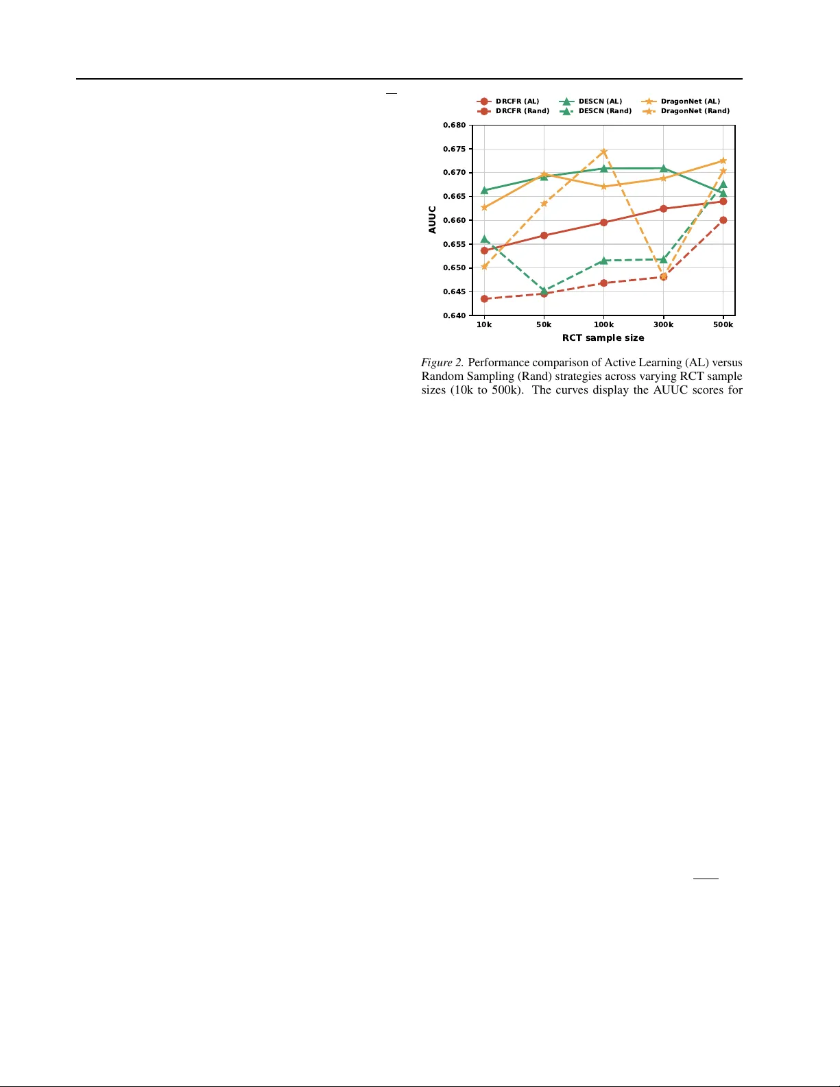
Budgeted Activ e Experimentation f or T r eatment Effect Estimation from Observ ational and Randomized Data Jiacan Gao * 2 Xinyan Su * 1 Mingyuan Ma 3 Y iyan Huang 4 Xiao Xu 1 Xinrui W an 1 Tianqi Gu 1 Enyun Y u 1 Jiecheng Guo 1 Zhiheng Zhang 5 6 Abstract Estimating heterogeneous treatment ef fects is cen- tral to data-driv en decision-making, yet industrial applications often face a fundamental tension be- tween limited randomized controlled trial (RCT) budgets and abundant but biased observational data collected under historical tar geting policies. Although observ ational logs of fer the adv antage of scale, they inherently suffer from se vere policy- induced imbalance and overlap violations, render- ing standalone estimation unreliable. W e propose a budgeted active experimentation frame work that iterativ ely enhances model training for causal ef- fect estimation via acti ve sampling. By lev eraging observational priors, we de velop an acquisition function targeting uplift estimation uncertainty , ov erlap deﬁcits, and domain discrepanc y to se- lect the most informati ve units for randomized experiments. W e establish ﬁnite-sample deviation bounds, asymptotic normality via martingale Cen- tral Limit Theorems (CL Ts), and minimax lower bounds to prove information-theoretic optimal- ity . Extensive experiments on industrial datasets demonstrate that our approach signiﬁcantly out- performs standard randomized baselines in cost- constrained settings. 1. Introduction Estimating heterogeneous treatment effects (HTE), such as the conditional a verage treatment effect (CA TE), is a cen- * Equal contribution 1 Didi Chuxing, Beijing, China 2 School of Statistics, East China Normal Univ ersity , Shanghai, China 3 School of Mathematics and Statistics, Beijing Jiaotong Uni versity , Beijing, China 4 School of Computing and Information T echnol- ogy , Great Bay Univ ersity, Guangdong, China 5 School of Statis- tics and Data Science, Shanghai University of Finance and Eco- nomics, Shanghai 200433, P .R. China 6 Institute of Data Science and Statistics, Shanghai University of Finance and Economics, Shanghai 200433, P .R. China. Correspondence to: Zhiheng Zhang < zhangzhiheng@mail.shufe.edu.cn > . Pr eprint. F ebruary 26, 2026. tral problem in causal inference and data-dri ven decision making. Accurate HTE estimation underpins personalized marketing, recommendation systems, clinical decision sup- port, and public policy design, where decisions must be tailored to individual characteristics rather than population av erages. In large-scale real-world systems, ho we ver , HTE estimation is constrained by a fundamental asymmetry in data sources: randomized controlled trials (RCTs) provide unbiased and reliable causal signals, but are expensiv e, slo w to deploy , and sev erely limited in sample size; observ ational data (OBS), in contrast, are ab undant and high-dimensional, but are generated under historical tar geting policies that in- duce selection bias, policy-driv en imbalance, and violations of ov erlap ( Hatt et al. , 2022 ; Colnet et al. , 2024 ). This asymmetry has moti v ated a gro wing literature on learn- ing treatment ef fects from multiple data sources. Classical work focuses on causal identiﬁcation from observ ational data under strong assumptions such as ignorability and posi- tivity , while more recent approaches seek to combine OBS and RCT data through reweighting or doubly robust estima- tors ( Cheng & Cai , 2021 ). In industrial settings, howe ver , these approaches face a critical limitation: historical policies are often near-deterministic, creating regions of the cov ari- ate space where observ ational data provide essentially no counterfactual information. In such regimes, directly using OBS outcomes for identiﬁcation is potentially unreliable, while running large-scale uniform RCTs is prohibiti vely costly . This tension naturally shifts the focus from estimation to experiment design . Rather than asking how to e xtract causal effects from biased observational logs, a more operational question is: given ab undant observational data and a strict budg et for randomized e xperiments, wher e should one run RCTs to most ef ﬁciently learn heter ogeneous tr eatment ef- fects? This question lies at the intersection of causal infer - ence and acti ve learning, but differs fundamentally from classical acti ve learning: here, querying a unit does not merely rev eal a label, but requires acti vely assigning a treat- ment and observing a causal outcome. Existing acti ve learning approaches ha ve explored this prob- lem from two largely separate perspecti ves. One line of 1 Budgeted Active Experimentation f or T reatment Effect Estimation from Observ ational and Randomized Data work studies acti ve or b udgeted sampling within experimen- tal settings ( Zhang et al. , 2025 ; Kato et al. , 2024 ; Ghadiri et al. , 2023 ), where treatments can be freely assigned but the RCT sample size is limited. Another line focuses on ac- tiv e learning within observational studies ( W en et al. , 2025 ; Gao et al. , 2025 ), where treatment assignments are ﬁxed and the budget corresponds to labeling or outcome acqui- sition. In contrast, the practically relev ant regime where observational data and experimental design coe xist — abun- dant biased logs alongside a small, adapti vely collected RCT— has receiv ed comparati vely little theoretical and methodological attention. In particular , it remains unclear how observ ational data should guide adaptiv e experiment design while retaining ﬁnite-sample v alidity and statistical inference guarantees. In this paper , we propose a budgeted active e xperimentation frame work that addresses this gap by cleanly separating the roles of observ ational and randomized data. The core idea is that observational data inform e xperiment design, while randomized e xperiments pr ovide causal estimation . Specif- ically , observ ational logs are used to learn a shared repre- sentation, to diagnose overlap deﬁcits induced by historical policies, and to identify cov ariate regions under -represented in the current experimental sample. These signals are com- bined into a multi-criteria acquisition function that acti vely selects which units to enroll into RCTs. The ﬁnal estimator , howe ver , is identiﬁed purely by randomized experiments, ensuring robustness to arbitrary confounding in the observ a- tional source. This design induces a nontrivial statistical regime: the ex- perimental data are adapti vely collected, non-i.i.d., and de- pend on past outcomes. W e show that, despite adaptivity , randomization induces a martingale structure that protects unbiasedness, while activ e sampling shapes the information matrix and governs statistical efﬁcienc y . Perhaps counter - intuitiv ely , we prov e that e ven the most aggressiv e acti ve experimentation strate gy cannot beat a p d/B rate in gen- eral, where d is the effecti ve dimension of heterogeneity and B is the RCT budget. Acti ve learning does not create information out of thin air , but it can substantially improv e constants by repairing ov erlap and stabilizing the design. Our main contributions are summarized as follo ws: (i) W e propose a principled framew ork for budgeted ac- tiv e e xperimentation that integrates observational and ran- domized data by separating experiment design from causal identiﬁcation. (ii) W e provide a comprehensiv e theoretical analysis for adaptiv ely collected RCT data, including ﬁnite-sample de- viation bounds, asymptotic normality via martingale CL Ts, and minimax lower bounds establishing near -optimality . (iii) W e clarify of the precise role of observ ational data in Ep istem ic Un ce rta inty Acc umu late d RC T Data ( ) Repr ese ntation Learning ( ) Obs er vational Data ( ) CA TE Estimator ( ) Un label ed Can did ate Pool Th e CA TE Lear ner Model M ulti - Criter ia Acquisitio n Funct io n Sele ct T op - Batch ( ) Exec ute RC T & Obs er ve Outcome s ( ) Ad aptive Datas et Up date Domain Discr epancy Ove rl ap Defi ci t Ca ndida tes for RCT Selection Ca libra te Confounding Abunda nt Superv isio n F igur e 1. Overview of the proposed Budgeted Active Exper - imentation framework for OBS-RCT fusion. W e ﬁrst train a CA TE learner using abundant observ ational logs, then iterati vely select a small batch of units from an unlabeled candidate pool D po ol for randomized experiments under a ﬁx ed b udget. At each iteration, a multi-criteria acquisition function S ( u ) scores and ranks candidates by balancing three signals: epistemic uncer - tainty ( v u ), domain discrepancy ( d u ), and ov erlap deﬁcit ( o u ). W e select the top-ranked units to run RCTs, add the new outcomes to the labeled set, and update the learner to reduce CA TE estima- tion error . causal learning: OBS improv es where to randomize, not what is identiﬁed, yielding a robust and interpretable path to cost-efﬁcient HTE estimation. The remainder of the paper is organized as follows. Sec- tion A re vie ws related work on acti ve learning and treat- ment effect estimation. Section 2 formalizes the two-source causal learning problem. Section 3 presents the proposed activ e experimentation algorithm. Section 4 develops the theoretical guarantees under adapti ve, non-i.i.d. e xperimen- tation. Section 5 reports empirical results on lar ge-scale real-world data. Section 6 concludes with implications and future directions. 2. Problem F ormulation Notation. Uppercase letters denote random variables and lowercase denote their realizations. Let X ∈ X ⊆ R d be cov ariates, T ∈ { 0 , 1 } a binary treatment, and Y ∈ { 0 , 1 } a binary outcome (the formulation ext ends to any bounded Y ∈ [0 , 1] ). For any distrib ution Q , we write E Q [ · ] and P Q ( · ) for expectation and probability under Q . W e adopt the Neyman–Rubin potential outcomes frame work ( Rubin , 2005 ). Each unit has potential outcomes Y (1) and Y (0) under treatment and control, respecti vely . The observed outcome follows Y = Y ( T ) . Assumption 2.1. (SUTV A). (i) No interfer ence : a unit’ s po- tential outcomes are unaffected by other units’ assignments. (ii) Consistency : Y = T Y (1) + (1 − T ) Y (0) . For the tar get estimand and e valuation metric , our estimand is the conditional av erage treatment effect (CA TE) ( Shalit et al. , 2017 ; Zhong et al. , 2022 ; Gao et al. , 2025 ): τ ( x ) = E [ Y (1) − Y (0) | X = x ] , x ∈ X . (1) 2 Budgeted Active Experimentation f or T reatment Effect Estimation from Observ ational and Randomized Data Deﬁne µ t ( x ) ≜ E [ Y ( t ) | X = x ] for t ∈ { 0 , 1 } , so that τ ( x ) = µ 1 ( x ) − µ 0 ( x ) . W e e valuate generalization over a tar get population whose cov ariate mar ginal distribution is P X . Given an estimator ˆ τ , we use the PEHE-style risk ( Hill , 2011 ; W en et al. , 2025 ; Gao et al. , 2025 ): R ( ˆ τ ) ≜ p E X ∼ P X [( ˆ τ ( X ) − τ ( X )) 2 ] . (2) W e hav e access to two-source data: (i) Observa- tional log (OBS). An observ ational dataset D obs = { ( X obs i , T obs i , Y obs i ) } n obs i =1 i . i . d . ∼ P obs , collected under a his- torical (possibly non-random) assignment polic y . Let the in- duced observ ational propensity be e obs ( x ) ≜ P obs ( T obs = 1 | X obs = x ) , which may be highly imbalanced and e ven (nearly) deterministic in some regions. W e write P obs as shorthand for P P obs . (ii) Unlabeled candidate pool (RCT -POOL). An unlabeled pool D po ol = { X po ol j } n po ol j =1 i . i . d . ∼ P X , from which we may query a small subset of units to run randomized e xperiments. Units in D po ol receiv e no treatment unless queried. Because OBS treatments follo w a historical polic y , global positivity in D obs (i.e., 0 < e obs ( x ) < 1 for all x ) may fail. W e therefore do not assume global o verlap for OBS; instead, we will use randomized experiments on queried units to obtain counterfactual information in weak(non)- ov erlap regions. Moreov er , we view D po ol = { X po ol j } n po ol j =1 as an unlabeled sample from the targ et covariate marginal P X , whereas D obs = { ( X obs i , T obs i , Y obs i ) } n obs i =1 is drawn from a dif fer - ent joint law P obs induced by a historical (possibly near- deterministic) targeting policy . Accordingly , the cov ariate marginals need not match: in general P X obs  = P X and supp( P X obs ) ⊆ supp( P X ) , reﬂecting selection bias and potential ov erlap violations in the observational log. Our design therefore treats D po ol as the population whose risk is ev aluated, while using D obs only to guide where to ran- domize (and not for causal identiﬁcation in weak-o verlap regions). Active Experimentation Protocol (Adaptive RCT). W e sequentially run experiments for K rounds (or until the budget is e xhausted). Let D (0) rct = ∅ initially . At round k , an adaptiv e strate gy selects an index set C k ⊆ [ n po ol ] from the remaining pool. For each selected unit with cov ariate X , we assign treatment T rct ∼ Bern  p k ( X )  , p k : X → [ f min , f max ] , where the randomization probability p k ( · ) is known and satisﬁes 0 < f min ≤ f max < 1 . W e then observe Y rct and record the quadruple ( X, T rct , Y rct , p k ( X )) . The experimental dataset is updated as D ( k ) rct ← D ( k − 1) rct ∪{ ( X po ol j , T rct j , Y rct j , p k ( X po ol j )) : j ∈ C k } . (3) Since C k and p k ( · ) may depend on the history , D ( k ) rct is adap- tiv ely collected and thus non-i.i.d. Assumption 2.2. (Randomization and positi vity in RCT). Conditioned on the history up to round k and cov ariates X , the RCT assignment is randomized: T rct ⊥ ( Y (0) , Y (1)) | ( X, history ) and P ( T rct = 1 | X, history ) = p k ( X ) ∈ [ f min , f max ] . Assumption 2.3. (Outcome in variance across sources). The conditional potential outcome distributions are shared across sources: for each t ∈ { 0 , 1 } and x ∈ X , P obs  Y ( t ) | X = x  = P X  Y ( t ) | X = x  . Equiv alently , the target CA TE τ ( x ) is common to both sources. Assumption 2.4. (Ignorability for OBS; used when le ver - aging OBS causally). When we use OBS for causal identiﬁ- cation (e.g., via propensity-based corrections), we assume conditional ignorability : ( Y (0) , Y (1)) ⊥ T obs | X obs un- der P obs . Objective. Let π denote an adaptive experiment design that generates the sequence { ( C k , p k ) } k ≥ 1 based on the ob- served history . Gi ven a total experimental budget B (the number of queried units), we aim to design π and a corre- sponding estimator ˆ τ π trained using both D obs and D ( K ) rct such that the target risk ( 2 ) is minimized: min π R  ˆ τ π  s.t. K X k =1 |C k | ≤ B . (4) Equiv alently , one may consider the sample complex- ity N RCT ( ε ) : the minimum b udget required to achieve R ( ˆ τ π ) ≤ ε with high probability . Assumptions 2.1 – 2.4 are standard in causal learning but play distinct roles here: (i) SUTV A ensures a well-deﬁned unit-lev el causal model; (ii) Assumption 2.2 guarantees unbiased identiﬁcation from queried RCT samples and pre- vents e xtreme-variance estimators via [ f min , f max ] ; (iii) As- sumption 2.3 enables pooling information across sources (diagnosable by comparing cov ariate distributions and out- come model residuals across domains); (i v) Assumption 2.4 is only needed if OBS is used for causal correction—if it is questionable, OBS can be used more conserv ativ ely (e.g., for representation learning / warm-starting), while identi- ﬁcation and calibration rely primarily on the randomized samples. 3. Methodology W e study a two-source setting where (i) a lar ge observa- tional log D obs provides ab undant but potentially biased and weak-ov erlap supervision, and (ii) an unlabeled pool D po ol represents the target population from which we may enroll a small number of units into randomized experiments. Our objecti ve is to lev erage a limited e xperimental b udget 3 Budgeted Active Experimentation f or T reatment Effect Estimation from Observ ational and Randomized Data Algorithm 1 Activ e Sampling for OBS-RCT Fusion Require: Observational Data D obs , Unlabeled Pool D po ol , Max Query Batch Size M , Budget B , Max Rounds K . Ensure: Final CA TE Estimator ˆ τ π . 1: Initialize: D rct ← ∅ , k ← 1 . 2: Representation Learning: T rain feature encoder ϕ : X → H on D obs ∪ D po ol . 3: while |D rct | < B and k ≤ K do 4: m k ← min( M , B − |D rct | ) 5: 1. Update Scoring Components: 6: T rain domain classiﬁer g ξ ( ϕ ( x )) to discriminate D po ol (label 1) from D obs ∪ D rct (label 0). 7: Update CA TE predictions M = { ˆ τ j ( x ) } E j =1 . { E : # of stochastic passes } 8: Estimate propensity ˆ e obs ( ϕ ( x )) ≈ P obs ( T obs = 1 | ϕ ( x )) 9: 2. Acquisition Scoring: 10: for candidate u ∈ D po ol do 11: v u ← V ar  { ˆ τ j ( ϕ ( u )) } E j =1  12: d u ← σ ( g ξ ( ϕ ( u ))) { σ ( · ) : Sigmoid Function } 13: o u ← 2 · | ˆ e obs ( ϕ ( u )) − 0 . 5 | 14: Compute Score: { η ( · ) : Rank Function } 15: S ( u ) ← α · η ( v u ) + β · η ( d u ) + γ · η ( o u ) 16: end for 17: 3. Selection & Experimentation: 18: Select candidates C k ← T op- m k ( S ( · ) , D po ol ) . 19: for X i ∈ C k do 20: Perform RCT : Assign T rct i ∼ Bern( p k ( X i )) , ob- serve Y rct i . 21: D rct ← D rct ∪ { ( X i , T rct i , Y rct i , p k ( X i )) } . 22: end for 23: 4. Update: D po ol ← D po ol \ C k ; k ← k + 1 . 24: end while 25: Return ˆ τ π trained on D obs ∪ D rct . B to acquire an adaptiv ely designed RCT dataset D rct , and then learn a ﬁnal CA TE estimator ˆ τ π from the augmented data D obs ∪ D rct . The key difﬁculty is wher e to run RCTs. Running e xperi- ments uniformly at random wastes budget on regions where OBS already provides reliable information, while failing to repair regions where OBS is systematically uninforma- tiv e (e.g., extreme propensities) or where the learned model extrapolates. W e therefore cast experiment design as a pool- based active learning problem for causal effect estimation: each queried unit provides both a randomized treatment as- signment and an outcome label, which can directly reduce CA TE error . Algorithm 1 summarizes our procedure. Below we explain the intuition behind each module, focusing on three canonical sources of CA TE estimation error that are particularly sev ere in OBS–RCT fusion: (i) Epistemic uncertainty of the CA TE model due to ﬁnite data and high-dimensional cov ariates; (ii) Domain discrepancy between the biased OBS log and the acti vely collected RCT sample (and thus the tar get pool); (iii) Overlap deﬁcit in OBS, where near-deterministic historical targeting makes counterfactual information essentially absent. Each error source is addressed by an explicit design choice: cov ariate shift is handled by querying from the unlabeled pool D po ol to restore coverage of the tar get mar ginal P X ; weak or missing overlap is mitigated by targeted random- ization rather than reweighting observ ational outcomes; and adaptivity bias is controlled by design-based randomiza- tion guarantees. Here, uncertainty refers not only to esti- mation variance conditional on a ﬁxed design, but also to design-induced uncertainty arising from which regions of the covariate space recei ve randomized e vidence. Our activ e strategy reduces this uncertainty by allocating experimental budget to co variate re gions with the largest mar ginal contri- bution to CA TE risk, yielding tighter error bounds for a ﬁx ed RCT cost. As a result, uncertainty is activ ely shaped—and prov ably reduced—by the experimental design, rather than passiv ely inherited from OBS–RCT fusion. Our acquisi- tion score explicitly combines proxies for these three error sources, so that each RCT query yields maximal marginal value to ward reducing the target PEHE risk. T o mitigate instability in high-dimensional industrial set- tings, we employ a shared Multilayer Perceptron (MLP) encoder , deﬁned as ϕ : X → H , to map raw cov ariates into a dense latent representation. This shared backbone serves as a common foundation for (i) propensity estimation, (ii) CA TE modeling, and (iii) domain discrimination, so that all components operate in a uniﬁed lower -dimensional space. v u : Backbone CA TE learner and ensemble for uncer- tainty . Since single causal models typically underestimate epistemic uncertainty ( T oth et al. , 2022 ), we rely on en- semble disagreement to quantify the lack of knowledge. While such disagreement can be captured via Deep Ensem- bles ( Lakshminarayanan et al. , 2017 ), we employ Monte Carlo (MC) Dropout ( Gal & Ghahramani , 2016 ) for compu- tational efﬁcienc y . W e perform E stochastic forward passes to obtain a set of CA TE predictions { ˆ τ j } E j =1 . The uncer- tainty score is deﬁned as the variance of these estimates: v u ≜ V ar  { ˆ τ j ( ϕ ( u )) } E j =1  (5) A large v u implies signiﬁcant disagreement among the stochastic sub-models, indicating that querying u yields high information gain by reducing epistemic uncertainty . d u : Domain discrimination for repr esentativ eness and distributional alignment. T o prevent the acti ve set from 4 Budgeted Active Experimentation f or T reatment Effect Estimation from Observ ational and Randomized Data drifting solely tow ards decision boundaries and to mitigate the selection bias inherent in D obs , we explicitly enforce distributional alignment. W e employ a domain classiﬁer g ξ operating on the representation space, trained to distinguish the target pool D pool from the current training set D current = D obs ∪ D rct . The score is deﬁned as the predicted probability of belonging to the target pool (label 1): d u ≜ P ( domain = 1 | ϕ ( u ); ξ ) = σ ( g ξ ( ϕ ( u ))) (6) where g ξ ( · ) denotes the logit output and σ ( · ) is the sigmoid function. Theoretically , g ξ acts as a density-ratio estimator where the logit approximates log( p pool ( ϕ ) /p current ( ϕ )) . Con- sequently , prioritizing high d u targets samples in regions under-represented by the current source data, minimizing cov ariate shift and ensuring robust generalization. o u : Propensity-based overlap deﬁcit fr om OBS. T o miti- gate estimator instability caused by e xtreme observ ational propensities (positi vity violations), we e xplicitly tar get re- gions lacking common support. W e utilize a propensity model ˆ e obs ( ϕ ( u )) ≈ P obs ( T obs = 1 | ϕ ( u )) , pre-trained on D obs , to deﬁne the deﬁcit score: o u ≜ 2 · | ˆ e obs ( ϕ ( u )) − 0 . 5 | . Samples with high o u correspond to regions where the historical policy was deterministic. Prioritizing these instances for RCT labeling ef fecti vely “repairs” the over - lap deﬁcit by injecting counterfactual information exactly where the observational signal is weak est. Rank-Normalized Multi-Criteria Acquisition Function. The three signals ( v u , d u , o u ) can hav e very dif ferent scales and may change ov er rounds. Instead of brittle scale- dependent normalization, we use a simple rank-based map η ( · ) , computed ov er the current pool: η ( a u ) ≜ 1 |D po ol | P u ′ ∈D po ol I ( ψ ( a u ′ ) ≤ ψ ( a u )) ∈ [0 , 1] , where ψ ( · ) is a monotone transform used for ranking. Since the con- structed signals v u , d u , and o u are all non-negativ e and positiv ely correlated with the informativ eness of a sample, we simply use identity transform ψ ( a ) = a for ranking. F or each pool candidate u , we compute acquisition score: S ( u ) ≜ α · η ( v u ) + β · η ( d u ) + γ · η ( o u ) , (7) and select the top- m k candidates. α, β , and γ balance the trade-off between uncertainty , discrepancy , and counter - factual co verage. T o ensure scale consistency across these heterogeneous metrics, we apply rank normalization prior to weighted aggregation. 3.1. Adaptive RCT execution and dataset update After selecting C k , we conduct randomized experiments for each X i ∈ C k . W e allo w a cov ariate-dependent randomization policy f k ( · ) (e.g., to incorporate opera- tional constraints), and enforce positi vity by clipping: p i ≜ Clip( f k ( X i ) , f min , f max ) , where Clip( z , a, b ) ≜ min { max { z , a } , b } . W e then draw T i ∼ Bern( p i ) , observ e Y i , and update as in ( 3 ) . Storing p i is essential for down- stream learning/inference when randomization probabilities are not constant. Finally , we remove C k from D po ol and repeat until the budget is e xhausted. W e reduce the selection of optimal p in Proposition B.15 . 4. Theoretical Analysis This section provides theoretical guarantees for the estima- tion component of Algorithm 1 under the adaptively col- lected RCT data. Our goal is to make three claims precise: (i) Finite-sample validity : an (near -) unbiased ef fect esti- mator and a non-asymptotic error bound that remains valid under adaptive, non-i.i.d. RCT sampling. (ii) Asymptotic inference : a central limit theorem (CL T) showing asymp- totic normality enabling conﬁdence interv als. (iii) Funda- mental limits : a minimax lo wer bound sho wing that the achiev ed rate is information-theoretically optimal (up to logs). A ke y theme is that randomization protects unbiased- ness, while acti ve selection shapes the information matrix and hence the error rate. W e ﬁrst formalize an analyzable estimator that matches the RCT protocol in Algorithm 1 and is standard in modern causal ML: regress an ortho gonalized pseudo-outcome onto a representation. A tractable estimator for adapti vely collected RCT sam- ples Let B denote the total RCT b udget and index queried units in chronological order t = 1 , . . . , B . Write the t -th queried sample as ( X t , T t , Y t , p t ) where p t ∈ [ f min , f max ] is the (known) assignment probability used when unit t was experimented. Let {F t } t ≥ 0 be the ﬁltration where F t con- tains D obs , the full cov ariate pool D po ol , and all RCT data up to time t . The adaptive querying policy (via C k , f k ) im- plies that X t and p t may depend on F t − 1 . W e deﬁne the RCT pseudo-outcome e Y t ≜ T t Y t p t − (1 − T t ) Y t 1 − p t . Intuiti vely , e Y t con v erts each single randomized trial into a noisy but unbiased “label” of the treatment effect at X t . Let ϕ ( x ) ∈ R d be a ﬁxed feature map (e.g., the learned embedding ϕ in Algorithm 1 ). For theory , we analyze a realizable linear CA TE model in this representation: τ ( x ) = ⟨ θ ⋆ , ϕ ( x ) ⟩ , θ ⋆ ∈ R d . This assumption is a stan- dard and useful “microscope”: it isolates the statistical dif- ﬁculty caused by adaptive designs + small budgets , while keeping the analysis transparent. (When τ ( · ) is not exactly linear , the bounds below become bounds on the best linear approximation plus an approximation error term.) Given { ( X t , T t , Y t , p t ) } B t =1 , we estimate θ ⋆ by (optionally re gu- larized) least squares on pseudo-outcomes: b θ λ ≜ arg min θ ∈ R d B X t =1  e Y t − ⟨ θ , ϕ ( X t ) ⟩  2 + λ ∥ θ ∥ 2 2 , (8) and output b τ λ ( x ) ≜ ⟨ b θ λ , ϕ ( x ) ⟩ . 5 Budgeted Active Experimentation f or T reatment Effect Estimation from Observ ational and Randomized Data Algorithm 2 Orthogonalized Linear CA TE Estimation on Adaptiv e RCT Data 1: Input: Adaptive RCT data { ( X t , T t , Y t , p t ) } B t =1 , fea- ture map ϕ ( · ) , ridge λ ≥ 0 . 2: Output: CA TE estimator b τ λ ( · ) . 3: for t = 1 , . . . , B do 4: Compute pseudo-outcome e Y t ← T t Y t p t − (1 − T t ) Y t 1 − p t . 5: end for 6: Form V λ ← λI d + P B t =1 ϕ ( X t ) ϕ ( X t ) ⊤ and b ← P B t =1 ϕ ( X t ) e Y t . 7: Solve b θ λ ← V − 1 λ b . 8: Return b τ λ ( x ) ← ⟨ b θ λ , ϕ ( x ) ⟩ . Algorithm 1 speciﬁes how the X t ’ s ar e chosen (activ e sam- pling) and how p t is assigned (bounded randomization). Algorithm 2 speciﬁes a transparent estimator for analyz- ing the statistical consequences of that adapti ve design. In practice, one may replace the linear re gressor by a neural CA TE learner; the ke y objects in the proofs belo w are (i) the unbiased pseudo-outcome, and (ii) an information ma- trix that quantiﬁes how well the queried points cover the representation space. Role of observational data in the estimator . It is impor- tant to clarify that the causal identiﬁcation of τ ( x ) is carried exclusi vely by randomized experiments. Observ ational data are not directly used in the estimating equations. Instead, D obs enters the procedure in tw o structural ways: (i) it de- ﬁnes the representation ϕ ( · ) in which the CA TE is approxi- mated, and (ii) it shapes the adapti ve experiment design that determines the queried cov ariates { X t } B t =1 . All theoretical guarantees are therefore design-adaptive but identiﬁcation- r obust : they remain valid e ven when the observational as- signment mechanism is arbitrarily confounded. 4.1. Unbiasedness and ﬁnite-sample error bounds W e now state the ﬁrst main result: despite adaptive (non- i.i.d.) selection of X t , the RCT pseudo-outcome remains unbiased, which implies unbiasedness of the linear estimator (for λ = 0 ) and a sharp ﬁnite-sample de viation bound (for any λ ≥ 0 ). Assumption 4.1. (Predictable adapti ve design). For each t , the queried cov ariate X t and assignment probability p t are F t − 1 -measurable. Assumption 4.2. (RCT randomization and boundedness). Conditioned on ( X t , p t , F t − 1 ) , treatment is randomized as T t ∼ Bern( p t ) and T t ⊥ ( Y t (0) , Y t (1)) | ( X t , p t , F t − 1 ) . Outcomes are bounded: Y t (0) , Y t (1) ∈ [0 , 1] almost surely , and p t ∈ [ f min , f max ] with 0 < f min ≤ f max < 1 . Assumption 4.3. (Linear realizability in representation space). There e xists θ ⋆ ∈ R d such that τ ( x ) = ⟨ θ ⋆ , ϕ ( x ) ⟩ for all x . Moreover , ∥ θ ⋆ ∥ 2 ≤ S and ∥ ϕ ( x ) ∥ 2 ≤ L for all x . Lemma 4.4 (Unbiased pseudo-outcome under adapti ve sam- pling) . Under Assumptions 4.1 – 4.2 , E h e Y t | X t , p t , F t − 1 i = τ ( X t ) , t = 1 , . . . , B . (9) | e Y t | ≤ max n 1 f min , 1 1 − f max o ≜ L p . Equation ( 9 ) says: even if we cherry-pick who enters the experiment , as long as we randomize treatment for the se- lected unit, each queried unit yields an unbiased, single- sample estimate of its own CA TE. A concrete e xample is coupon deli very: even if we actively choose “hard” users (e.g., high-v alue users with extreme historical targeting), a randomized coupon/no-coupon decision still produces an unbiased causal contrast at that user . This lemma is not claiming that the observ ational estimator is unbiased, nor that any neural training procedure is unbiased. It only uses RCT randomization and boundedness. The adapti ve selec- tion affects wher e we learn (which X t ’ s), not whether a queried unit is causally valid. A potential skeptic is that “But the learner chooses X t based on past outcomes; isn’t this a form of selection bias that breaks unbiasedness?” Response: the selection changes the distribution of X t , but unbiasedness in ( 9 ) is conditional on ( X t , p t , F t − 1 ) . The key is that T t is randomized af- ter selection and is conditionally independent of potential outcomes. T echnically , e Y t − τ ( X t ) forms a martingale dif- ference sequence. Under this preparation, we introduce the ﬁnite-sample bound as follows: Theorem 4.5 (Finite-sample unbiasedness and devia- tion bound) . Assume 4.1 – 4.3 . Let V λ ≜ λI d + P B t =1 ϕ ( X t ) ϕ ( X t ) ⊤ and let b θ λ be deﬁned in ( 8 ) . Then: (i) (Conditional unbiasedness for OLS). If λ = 0 and V 0 is in vertible, then E h b θ 0 | { X t , p t } B t =1 i = θ ⋆ , E  b τ 0 ( x ) | { X t , p t } B t =1  = τ ( x ) , ∀ x. (High- probability self-normalized bound). F ix δ ∈ (0 , 1) and any λ ≥ 0 . Ther e exists a constant σ ≤ 2 L p (depending only on f min , f max and the boundedness of Y ) such that with pr obability at least 1 − δ ,   b θ λ − θ ⋆   V λ ≤ σ s 2 log det( V λ ) 1 / 2 det( λI d ) 1 / 2 δ | {z } stochastic term + √ λ S | {z } r e gularization bias . (10) Consequently , for every x ∈ X ,   b τ λ ( x ) − τ ( x )   ≤ β B ( δ ) · q ϕ ( x ) ⊤ V − 1 λ ϕ ( x ) , (11) wher e β B ( δ ) ≜ σ q 2 log det( V λ ) 1 / 2 det( λI d ) 1 / 2 δ + √ λS. Theorem 4.5 quantiﬁes a clean “budget ⇒ error” trade- off under adaptive experimentation: your estimation error 6 Budgeted Active Experimentation f or T reatment Effect Estimation from Observ ational and Randomized Data is controlled by an information matrix V λ built from the queried cov ariates. The only price paid for adapti vity is that the X t ’ s are not i.i.d.; the deviation bound still holds because the noise is a martingale dif ference. It is easy to confuse ( 11 ) with classical i.i.d. regression bounds. The cru- cial dif ference is: the X t ’ s can be adversarially chosen by the learner itself, based on past outcomes. Theorem 4.5 re- mains v alid in that setting; it does not require i.i.d. sampling of X t . Notew orthy , in v ery small B , V 0 can be ill-conditioned. This is exactly why we stated ( 10 ) for ridge λ > 0 as well: the bound decomposes into a stochastic term plus an explicit r e gularization bias . This makes the tradeoff transparent and diagnosable in practice: if V 0 is poorly conditioned, increase λ to stabilize, and the theory tells you exactly how much bias you introduce. Corollary 4.6 (Finite-sample PEHE bound) . Under the conditions of Theor em 4.5 , with pr obability at least 1 − δ , R ( b τ λ ) ≤ β B ( δ ) · q E X ∼ P X  ϕ ( X ) ⊤ V − 1 λ ϕ ( X )  . (12) In particular , if the queried design is well-conditioned in the sense that V 0 ⪰ κB I d for some κ > 0 , and Σ X ≜ E P X [ ϕ ( X ) ϕ ( X ) ⊤ ] ⪯ L 2 I d , then (taking λ = 0 for simplicity), R ( b τ 0 ) ≤ β B ( δ ) · r T r(Σ X ) κB ≲ L σ √ κ r d log ( B /δ ) B . (13) Corollary 4.6 sho ws that the PEHE risk is gov erned by an inte gr ated levera ge term E P X [ ϕ ( X ) ⊤ V − 1 λ ϕ ( X )] . Acti ve sampling is useful precisely because it can shape V λ : se- lecting points that increase eigen v alues of V λ reduces this term. This provides a direct theoretical rationale for using an “uncertainty” proxy (Algorithm 1 , v u ): in linear mod- els, predictiv e v ariance is proportional to ϕ ( u ) ⊤ V − 1 λ ϕ ( u ) , and ensemble disagreement is a practical surrogate for that quantity . 4.2. Asymptotic normality under adaptive sampling Finite-sample concentration ensures “small error with high probability . ” For statistical inference (e.g., conﬁdence inter- vals), we further need a CL T . The non-i.i.d. nature of acti ve sampling prev ents a direct appeal to the classical i.i.d. CL T , but a martingale CL T applies. Assumption 4.7. (Stabilizing design and moments). As B → ∞ , the normalized information matrix con- ver ges in probability: 1 B P B t =1 ϕ ( X t ) ϕ ( X t ) ⊤ p − → Σ π , Σ π ≻ 0 . Moreov er , the conditional variances stabi- lize: 1 B P B t =1 E h  e Y t − τ ( X t )  2 ϕ ( X t ) ϕ ( X t ) ⊤    F t − 1 i p − → Ω π , and a Lindeberg condition holds for the martingale differences { e Y t − τ ( X t ) } t ≥ 1 . Theorem 4.8 (Asymptotic normality (martingale CL T)) . Suppose Assumptions 4.1 – 4.7 hold and λ = 0 . Then √ B  b θ 0 − θ ⋆  d = ⇒ N  0 , Σ − 1 π Ω π Σ − 1 π  . Consequently , for any ﬁxed x ∈ X , √ B  b τ 0 ( x ) − τ ( x )  d = ⇒ N  0 , ϕ ( x ) ⊤ Σ − 1 π Ω π Σ − 1 π ϕ ( x )  . Theorem 4.8 says: even though the RCT data ar e collected adaptively and ar e non-i.i.d., the ﬁnal estimator still ad- mits classical √ B -asymptotics. In practice, this supports uncertainty quantiﬁcation: one can estimate the sandwich variance Σ − 1 π Ω π Σ − 1 π from data and form approximate con- ﬁdence interv als for τ ( x ) at business-critical se gments (e.g., “new users” or “high-v alue users”). Notably , the technical challenge for constructing CL T be- yond i.i.d is the martingale structure created by randomiza- tion: e Y t − τ ( X t ) is conditionally mean-zero giv en the past. Assumption 4.7 requires that the design does not degener- ate (the information matrix stabilizes), which is exactly the failure mode acti ve learning must a void. This also clariﬁes why our acquisition score includes representati veness/shift terms ( d u ): they discourage pathological designs where Σ π becomes nearly singular . 4.3. Minimax lower bound and (near) optimality Upper bounds alone do not tell us whether a method is “the best possible. ” W e therefore complement them with a minimax lo wer bound. The message is intentionally sharp: e ven with perfect adaptivity and access to unlim- ited observational logs and unlabeled pools, one cannot beat the p d/B rate in gener al. Consider the linear class F lin ( S ) ≜  τ θ ( x ) = ⟨ θ , ϕ ( x ) ⟩ : θ ∈ R d , ∥ θ ∥ 2 ≤ S  . Assume P X puts equal mass on d cov ariate “types” { x (1) , . . . , x ( d ) } such that ϕ ( x ( j ) ) = e j (the j -th standard basis). This captures a realistic situation where the popula- tion is a mixture of d distinct segments and CA TE differs by segment. Theorem 4.9 (Minimax lo wer bound for activ e RCT un- der bounded randomization) . Under the har d instance de- scribed above, ther e exists a universal constant c > 0 such that for any adaptive querying policy π (possibly using D obs and D po ol ) and any estimator b τ based on B RCT samples, inf π inf b τ sup τ ∈F lin ( S ) E [ R ( b τ )] ≥ c · 1 f min (1 − f max ) q d B . Theorem 4.9 formalizes a simple but important reality: if there are d independent degrees of freedom in τ ( · ) (e.g., d user se gments with genuinely different causal responses), then with budget B you cannot estimate all of them faster than order p d/B in PEHE. Activ e learning can r eallocate samples to reduce constants, but it cannot create informa- tion out of thin air . It does not say that active sampling is 7 Budgeted Active Experimentation f or T reatment Effect Estimation from Observ ational and Randomized Data useless. It says that the best possible scaling in B is 1 / √ B for this class. Acti ve sampling is still v aluable because it improv es the information matrix (hence constants) and pre- vents de generacy , especially when OBS cov erage is heavily imbalanced. Corollary 4.10 (Near-minimax optimality of the orthogo- nalized estimator) . Under Assumptions 4.1 – 4.3 and a well- conditioned design V 0 ⪰ κB I d , the upper bound in ( 13 ) matches the minimax lower bound up to logarithmic factors and the conditioning constant κ . In this sense, the estimator in Algorithm 2 is minimax-rate optimal for F lin ( S ) . Also, we justify using f k ( x ) ≡ 1 / 2 as a default in Algo- rithm 1 could minimize the conditional variance, and using clipping [ f min , f max ] as a principled safeguard when p must vary by co variates. 5. Experiments Datasets. Our empirical e valuation utilizes a large-scale r eal-world dataset deri ved from a ride-hailing platform. The dataset is collected at the order lev el, with each instance corresponding to an indi vidual order characterized by 468 features. F ormally , let T ∈ { 0 , 1 } denote the treatment arm, indicating whether a “free upgrade” service was triggered for the passenger . Correspondingly , the outcome Y ∈ { 0 , 1 } is deﬁned as the order completion status. W e implement an Out-of-Time (OO T) protocol spanning 44 days. During the initial 30-day phase, we establish the RCT Pool D po ol and concurrently collect observ ational samples to form the training set (either D bias obs or D full obs ). Generalization is strictly ev aluated on the Unbiased RCT T est Set D test rct , which com- prises RCT data collected during the remaining 14 days. Detailed descriptions are provided in Appendix D.1 . Baselines & Metrics. In our experiments, we evaluate three industrial deep uplift baselines—DragonNet ( Shi et al. , 2019 ), DESCN ( Zhong et al. , 2022 ), and DRCFR ( Cheng et al. , 2022 )—under active v ersus random sampling. Due to the unobserv ability of counterfactuals in real-world indus- trial RCTs, direct calculation of PEHE is infeasible. Instead, we employ the Normalized Area Under the Uplift Curve (A UUC) ( Gutierrez & G ´ erardy , 2017 ), a practically-oriented metric widely adopted in industry to assess ranking quality . Main Results. W e demonstrate that the proposed active sampling strategy signiﬁcantly enhances sample ef ﬁciency in hybrid uplift modeling, maximizing the mar ginal utility of limited experimental data. As illustrated in Figure 2 , our approach yields consistent performance gains across all ev aluated architectures compared to random sampling. Speciﬁcally , the DRCFR model coupled with active sam- pling achieves an A UUC at 100k samples comparable to that of random sampling at 500k , ef fectiv ely reducing the RCT labeling cost by approximately 80% . For other backbones, 10k 50k 100k 300k 500k RCT sample size 0.640 0.645 0.650 0.655 0.660 0.665 0.670 0.675 0.680 A UUC DRCFR (AL) DRCFR (Rand) DESCN (AL) DESCN (Rand) DragonNet (AL) DragonNet (Rand) F igure 2. Performance comparison of Activ e Learning (AL) v ersus Random Sampling (Rand) strate gies across v arying RCT sample sizes (10k to 500k). The curves display the A UUC scores for DRCFR, DESCN, and DragonNet models. The experiments are conducted on the Biased Observational Set D bias obs , demonstrating the superior data efﬁcienc y of activ e sampling (solid lines) com- pared to random sampling (dashed lines) under distribution shifts. DESCN performs best at 10k , while DragonNet peaks at 500k . Notably , acti ve sampling stabilizes DragonNet by prev enting the large ﬂuctuations observed under random sampling. Supplementary results regarding data scalability , comprehensiv e ablation studies, and detailed experimental protocols are provided in Appendix F . 6. Conclusion W e study heterogeneous treatment effect estimation under a pervasi ve real-world constraint: randomized controlled trials are scarce and costly , while observ ational data are abundant b ut biased. In our frame work, observ ational data inform where randomized experimentation should occur, while causal identiﬁcation is carried e xclusiv ely by ran- domized experiments . W e formalize this perspecti ve as a budgeted activ e experimentation problem and propose a multi-criteria acquisition strate gy that le verages observ a- tional data to diagnose uncertainty , overlap deﬁcits, and cov ariate shift, thereby directing limited RCT budget to the most informativ e re gions. W e sho w that randomiza- tion induces a martingale structure that guarantees unbi- asedness, admits ﬁnite-sample deviation bounds, and yields asymptotic normality . Moreo ver , we establish minimax lower bounds demonstrating that the achie ved p d/B rate is information-theoretically optimal, clarifying that activ e learning improves efﬁciency through better experimental design rather than by circumventing fundamental limits. Furthermore, extending the theoretical guarantees beyond linear realizability to richer nonparametric or deep function 8 Budgeted Active Experimentation f or T reatment Effect Estimation from Observ ational and Randomized Data classes remains an important challenge, and jointly optimiz- ing unit selection and treatment randomization probabili- ties may further impro ve ef ﬁciency under operational con- straints. W e believ e these directions will further strengthen activ e e xperimentation as a foundational paradigm for cost- efﬁcient causal learning. 9 Budgeted Active Experimentation f or T reatment Effect Estimation from Observ ational and Randomized Data References Addanki, R., Arbour , D., Mai, T ., Musco, C., and Rao, A. Sample constrained treatment effect estimation. Ad- vances in Neural Information Pr ocessing Systems , 35: 5417–5430, 2022. Cheng, D. and Cai, T . Adaptiv e combination of randomized and observ ational data. arXiv pr eprint arXiv:2111.15012 , 2021. Cheng, M., Liao, X., Liu, Q., Ma, B., Xu, J., and Zheng, B. Learning disentangled representations for counterfac- tual regression via mutual information minimization. In Pr oceedings of the 45th International A CM SIGIR Con- fer ence on Researc h and Development in Information Retrieval , pp. 1802–1806, 2022. Colnet, B., Mayer, I., Chen, G., Dieng, A., Li, R., V aro- quaux, G., V ert, J.-P ., Josse, J., and Y ang, S. Causal inference methods for combining randomized trials and observ ational studies: a revie w . Statistical science , 39(1): 165–191, 2024. Gal, Y . and Ghahramani, Z. Dropout as a bayesian approx- imation: Representing model uncertainty in deep learn- ing. In international conference on mac hine learning , pp. 1050–1059. PMLR, 2016. Gao, E., Fa wkes, J., and Sejdinovic, D. Causal-epig: A prediction-oriented acti ve learning framework for cate estimation, 2025. URL 2509.21866 . Ghadiri, M., Arbour , D., Mai, T ., Musco, C., and Rao, A. B. Finite population regression adjustment and non- asymptotic guarantees for treatment effect estimation. Advances in Neural Information Pr ocessing Systems , 36: 74180–74212, 2023. Gutierrez, P . and G ´ erardy , J.-Y . Causal inference and up- lift modelling: A revie w of the literature. In Hardgrov e, C., Dorard, L., Thompson, K., and Douetteau, F . (eds.), Pr oceedings of The 3rd International Confer ence on Pre- dictive Applications and APIs , volume 67 of Pr oceedings of Machine Learning Resear ch , pp. 1–13. PMLR, 11–12 Oct 2017. Hatt, T ., Berre v oets, J., Curth, A., Feuerrie gel, S., and v an der Schaar , M. Combining observational and random- ized data for estimating heterogeneous treatment ef fects. arXiv pr eprint arXiv:2202.12891 , 2022. Hill, J. L. Bayesian nonparametric modeling for causal infer- ence. Journal of Computational and Graphical Statistics , 20(1):217–240, 2011. URL https://doi.org/10. 1198/jcgs.2010.08162 . Kato, M., Oga, A., Komatsubara, W ., and Inokuchi, R. Activ e adaptive experimental design for treatment ef- fect estimation with cov ariate choices. arXiv preprint arXiv:2403.03589 , 2024. Lakshminarayanan, B., Pritzel, A., and Blundell, C. Simple and scalable predictiv e uncertainty estimation using deep ensembles. Advances in neural information pr ocessing systems , 30, 2017. Rubin, D. B. Causal inference using potential outcomes: Design, modeling, decisions. Journal of the American statistical Association , 100(469):322–331, 2005. Shalit, U., Johansson, F . D., and Sontag, D. Estimating individual treatment ef fect: generalization bounds and algorithms. In International confer ence on machine learn- ing , pp. 3076–3085. PMLR, 2017. Shi, C., Blei, D. M., and V eitch, V . Adapting neural net- works for the estimation of treatment ef fects. In Advances in Neural Information Pr ocessing Systems , v olume 32, 2019. T oth, C., Lorch, L., Knoll, C., Krause, A., Pernkopf, F ., Peharz, R., and von K ¨ ugelgen, J. Acti ve bayesian causal inference. In Advances in Neural Information Pr ocess- ing Systems , volume 35, pp. 16261–16275. Curran Asso- ciates, Inc., 2022. W en, H., Chen, T ., Gong, M., Chai, L. K., Sadiq, S., and Y in, H. Enhancing treatment effect estimation via acti ve learning: A counterfactual covering perspectiv e, 2025. URL . Zhang, Z., W ang, H., Li, H., and Lin, Z. Acti ve treatment effect estimation via limited samples. In F orty-second International Confer ence on Machine Learning , 2025. Zhong, K., Xiao, F ., Ren, Y ., Liang, Y ., Y ao, W ., Y ang, X., and Cen, L. Descn: Deep entire space cross networks for individual treatment ef fect estimation. In Proceed- ings of the 28th ACM SIGKDD confer ence on knowledge discovery and data mining , pp. 4612–4620, 2022. Zhu, Y . and Now ak, R. Active learning with neural net- works: Insights from nonparametric statistics. Advances in Neural Information Pr ocessing Systems , 35:142–155, 2022. 10 Budgeted Active Experimentation f or T reatment Effect Estimation from Observ ational and Randomized Data A. Related W ork Industrial CA TE estimation often faces challenge: limited RCT budgets versus ab undant but biased observ ational data. This motiv ates us to dev elop an OBS & RCT data fusion frame work that casts experiment design as a budgeted acti ve learning problem. In this section, we discuss related work on (i) active sampling for budg et-limited experiments , (ii) active sampling in observational studies , and (iii) active learning with neural networks . (i) Active sampling f or budget-limited experiments. In sample-constrained RCT settings, the unlabeled pool is available but only a small subset of individuals can be enrolled, and the goal is to minimize estimation error via selecti ve recruitment. Addanki et al. ( 2022 ) utilize lev erage-based selection and balanced assignment to optimize A TE deviation under ﬁxed budgets. Similarly , Zhang et al. ( 2025 ) propose adaptive sampling with re weighting (R W AS) to achie ve stable, sample-ef ﬁcient A TE estimation within a limited draw b udget. (ii) Active sampling in obser vational studies. In observational settings, treatment is pre-assigned, and the budget restricts label queries. W en et al. ( 2025 ) prioritize enhancing factual and counterfactual coverag e to impro ve o verlap and reduce PEHE. Alternati vely , Causal-EPIG ( Gao et al. , 2025 ) employs an information-theoretic approach, selecting samples that maximize expected predicti ve information gain to minimize CA TE uncertainty under a limited labeling budget. (iii) Active lear ning with neural networks. In neural settings, acquisition is often dri ven by disagreement or uncertainty . Zhu & No wak ( 2022 ) propose NeuralCAL, which queries points in the disagr eement re gion of plausible predictors to reduce label complexity . Its extension, NeuralCAL++, further inte grates abstention mechanisms and conﬁdence intervals to reach target error rates with signiﬁcantly fe wer queries. T able 1. Comparison of related works in Activ e Learning (AL) for T reatment Ef fect Estimation. AL Methods Data Objective & Budget Guides Exp. Design? Acquisition Strategy Evaluation Metric Ours. (AL for RCT&OBS TE) OBS + RCT Obj: Min. CA TE Error Budget: RCT Ex- periment Budget ✓ Ours: T op- k by uncertainty + dis- crepancy + ov erlap deﬁcit. A UUC (For CA TE) Sample-Constrained TE Est. ( Addanki et al. , 2022 ) RCT only Obj: Min. A TE/ITE Error Budget: Limited Sample Size ✓ SCTE: T op- k infor- mativ e units with cov ariate-balanced assignment. RMSE (For ITE) Deviation (F or A TE) Activ e TE Est. ( Zhang et al. , 2025 ) RCT only Obj: Min. A TE Er - ror Budget: Limited Sample Size ✓ R W AS: Probability sampling + in verse- propensity reweight- ing. Deviation (F or A TE) Enhancing TE Est. ( W en et al. , 2025 ) OBS only Obj: Min. CA TE Error Budget: Labeling Budget ✗ Coverage: T op- k maximizing fac- tual/counterfactual cov erage. RMSE (For ITE) PEHE (For CA TE) Causal-EPIG ( Gao et al. , 2025 ) OBS only Obj: Min. CA TE Error Budget: Labeling Budget ✗ Causal-EPIG: T op- k by expected pre- dictiv e information gain. PEHE (For CA TE) AL with Neural Networks ( Zhu & Now ak , 2022 ) Supervised Obj: Optim. Label Complexity and Excess Error Budget: Query Count ✗ NeuralCAL(++): T op- k by disagree- ment/ambiguity (with abstention). Excess Error Label Complexity Note: OBS = Observ ational Data, RCT = Randomized Controlled T rial. Guides Exp. Design? : Indicates if the method actively assigns treatments ( ✓ ) or only queries labels ( ✗ ). 11 Budgeted Active Experimentation f or T reatment Effect Estimation from Observ ational and Randomized Data B. Theoretical Analysis This section provides theoretical guarantees for the estimation component of Algorithm 1 under the adaptively collected RCT data. Our goal is to make three claims precise: (i) Finite-sample validity : an (near-) unbiased effect estimator and a non-asymptotic error bound that remains valid under adaptive , non-i.i.d. RCT sampling. (ii) Asymptotic inference : a central limit theorem (CL T) showing asymptotic normality enabling conﬁdence intervals. (iii) Fundamental limits : a minimax lower bound sho wing that the achieved rate is information-theoretically optimal (up to logs). A key theme is that randomization pr otects unbiasedness, while active selection shapes the information matrix and hence the err or rate. W e ﬁrst formalize an analyzable estimator that matches the RCT protocol in Algorithm 1 and is standard in modern causal ML: regress an orthogonalized pseudo-outcome onto a representation. B.1. Setup: adaptive RCT stream and pseudo-outcome r egression Let B denote the total RCT budget and index queried units in chronological order t = 1 , . . . , B . Write the t -th queried sample as ( X t , T t , Y t , p t ) where p t ∈ [ f min , f max ] is the (kno wn) assignment probability used when unit t was experimented. Let {F t } t ≥ 0 be the ﬁltration where F t contains D obs , the full cov ariate pool D po ol , and all RCT data up to time t . The adaptiv e querying policy (via C k , f k ) implies that X t and p t may depend on F t − 1 . W e deﬁne the RCT pseudo-outcome e Y t ≜ T t Y t p t − (1 − T t ) Y t 1 − p t . (14) Intuitiv ely , e Y t con verts each single randomized trial into a noisy but unbiased “label” of the treatment ef fect at X t . Let ϕ ( x ) ∈ R d be a ﬁxed feature map (e.g., the learned embedding ϕ in Algorithm 1 ). For theory , we analyze a realizable linear CA TE model in this representation: τ ( x ) = ⟨ θ ⋆ , ϕ ( x ) ⟩ , θ ⋆ ∈ R d . (15) Giv en { ( X t , T t , Y t , p t ) } B t =1 , we estimate θ ⋆ by (optionally regularized) least squares on pseudo-outcomes: b θ λ ≜ arg min θ ∈ R d B X t =1  e Y t − ⟨ θ , ϕ ( X t ) ⟩  2 + λ ∥ θ ∥ 2 2 , (16) and output b τ λ ( x ) ≜ ⟨ b θ λ , ϕ ( x ) ⟩ . Algorithm 2 summarizes this estimator . Algorithm 1 speciﬁes how the X t ’ s ar e chosen (active sampling) and how p t is assigned (bounded randomization). Algorithm 2 isolates a transparent estimator for analyzing the statistical consequences of that adapti ve design. In practice, one may replace the linear regressor by a neural CA TE learner; the ke y objects in the proofs belo w are (i) the unbiased pseudo-outcome, and (ii) an information matrix that quantiﬁes how well the queried points co ver the representation space. B.2. Unbiasedness and ﬁnite-sample error bounds W e no w state the ﬁrst main result: despite adaptive (non-i.i.d.) selection of X t , the RCT pseudo-outcome remains unbiased, which implies unbiasedness of the linear estimator (for λ = 0 ) and a ﬁnite-sample de viation bound (for λ > 0 ). Assumption B.1. (Predictable adaptiv e design). For each t , the queried cov ariate X t and assignment probability p t are F t − 1 -measurable. Assumption B.2. (RCT randomization and boundedness). Conditioned on ( X t , p t , F t − 1 ) , treatment is randomized as T t ∼ Bern( p t ) and T t ⊥ ( Y t (0) , Y t (1)) | ( X t , p t , F t − 1 ) . Outcomes are bounded: Y t (0) , Y t (1) ∈ [0 , 1] almost surely , and p t ∈ [ f min , f max ] with 0 < f min ≤ f max < 1 . Assumption B.3. (Linear realizability in representation space). There exists θ ⋆ ∈ R d such that τ ( x ) = ⟨ θ ⋆ , ϕ ( x ) ⟩ for all x . Moreov er , ∥ θ ⋆ ∥ 2 ≤ S and ∥ ϕ ( x ) ∥ 2 ≤ L for all x . Lemma B.4 (Unbiased pseudo-outcome under adaptiv e sampling) . Under Assumptions 4.1 – 4.2 , E h e Y t | X t , p t , F t − 1 i = τ ( X t ) , t = 1 , . . . , B . (17) 12 Budgeted Active Experimentation f or T reatment Effect Estimation from Observ ational and Randomized Data Mor eover , e Y t is uniformly bounded: | e Y t | ≤ max  1 f min , 1 1 − f max  ≜ L p . (18) Pr oof. Fix t ∈ { 1 , . . . , B } . By consistency and Y t = T t Y t (1) + (1 − T t ) Y t (0) , T t Y t = T t Y t (1) , (1 − T t ) Y t = (1 − T t ) Y t (0) . Hence, e Y t = T t Y t (1) p t − (1 − T t ) Y t (0) 1 − p t . T aking conditional e xpectation gi ven ( X t , p t , F t − 1 ) and using Assumption 4.2 , E  T t Y t (1) p t     X t , p t , F t − 1  = E  E  T t p t     X t , p t , F t − 1 , Y t (1)  Y t (1)     X t , p t , F t − 1  = E  E [ T t | X t , p t , F t − 1 ] p t Y t (1)     X t , p t , F t − 1  = E [ Y t (1) | X t , p t , F t − 1 ] , where the second line uses conditional independence T t ⊥ Y t (1) | ( X t , p t , F t − 1 ) and the last line uses E [ T t | X t , p t , F t − 1 ] = p t . Similarly , E  (1 − T t ) Y t (0) 1 − p t     X t , p t , F t − 1  = E [ Y t (0) | X t , p t , F t − 1 ] . Therefore, E h e Y t | X t , p t , F t − 1 i = E [ Y t (1) − Y t (0) | X t , p t , F t − 1 ] = E [ Y t (1) − Y t (0) | X t ] = τ ( X t ) , where the second equality uses the randomization/ignorability in Assumption 4.2 and the last equality is the deﬁnition of CA TE. For boundedness, note that exactly one of the tw o terms in the pseudo outcome is nonzero: if T t = 1 , then e Y t = Y t /p t ∈ [0 , 1 /p t ] ; if T t = 0 , then e Y t = − Y t / (1 − p t ) ∈ [ − 1 / (1 − p t ) , 0] . Using p t ≥ f min and 1 − p t ≥ 1 − f max giv es ( 18 ). Equation ( 9 ) says: even if we cherry-pic k who enters the e xperiment , as long as we randomize treatment for the selected unit, each queried unit yields an unbiased, single-sample estimate of its own CA TE. A concrete example is coupon deli very: ev en if we actively choose “hard” users (e.g., high-value users with e xtreme historical targeting), a randomized coupon/no-coupon decision still produces an unbiased causal contrast at that user . This lemma is not claiming that the observ ational estimator is unbiased, nor that any neural training procedure is unbiased. It only uses RCT randomization and boundedness. The adaptiv e selection affects wher e we learn (which X t ’ s), not whether a queried unit is causally v alid. A potential skeptic is that “the learner chooses X t based on past outcomes; isn’ t this a form of selection bias that breaks unbiasedness?” The resolution is that unbiasedness in ( 9 ) is conditional on ( X t , p t , F t − 1 ) : the selection may change the distribution of X t , but T t is randomized after selection and is conditionally independent of potential outcomes. T echnically , e Y t − τ ( X t ) forms a martingale dif ference sequence. A key martingale object. Deﬁne the centered pseudo-outcome noise ε t ≜ e Y t − τ ( X t ) , (19) and the (predictable) feature vector ϕ t ≜ ϕ ( X t ) . By Lemma 4.4 , E [ ε t | F t − 1 , X t , p t ] = 0 and | ε t | ≤ 2 L p (since both e Y t and τ ( X t ) ∈ [ − 1 , 1] are bounded). Let V λ ≜ λI d + B X t =1 ϕ t ϕ ⊤ t , M B ≜ B X t =1 ϕ t ε t . (20) Then { M t } t ≥ 0 with M t = P t s =1 ϕ s ε s is a vector -v alued martingale with respect to {F t } . 13 Budgeted Active Experimentation f or T reatment Effect Estimation from Observ ational and Randomized Data A self-normalized concentration lemma (pro ved in full). The ﬁnite-sample bound relies on a vector-v alued self- normalized martingale inequality . Because this step is often cited as a black box, we provide a complete proof to make the non-i.i.d. aspect fully transparent. Lemma B.5 (Conditional sub-Gaussianity of ε t ) . Under Assumptions 4.1 – 4.2 , for each t and any λ ∈ R , E  exp  λ ε t    F t − 1 , X t , p t  ≤ exp  λ 2 σ 2 2  , with σ ≜ 2 L p . (21) Pr oof. Condition on ( F t − 1 , X t , p t ) . By Lemma 4.4 , E [ ε t | F t − 1 , X t , p t ] = 0 . Moreo ver , Y t ∈ [0 , 1] and p t ∈ [ f min , f max ] imply | e Y t | ≤ L p by ( 18 ) . Also τ ( X t ) = E [ Y (1) − Y (0) | X t ] ∈ [ − 1 , 1] because Y (1) , Y (0) ∈ [0 , 1] . Hence | ε t | ≤ | e Y t | + | τ ( X t ) | ≤ L p + 1 ≤ 2 L p since L p ≥ 1 . Now apply Hoeffding’ s lemma in conditional form: if Z is zero-mean and almost surely lies in [ a, b ] giv en a sigma-ﬁeld, then E [ e λZ | · ] ≤ exp( λ 2 ( b − a ) 2 / 8) . Here Z = ε t and [ a, b ] = [ − 2 L p , 2 L p ] , so ( b − a ) 2 / 8 = (4 L p ) 2 / 8 = 2 L 2 p . Thus ( 21 ) holds with σ = 2 L p . Lemma B.6 (Self-normalized martingale inequality (vector form)) . Assume λ > 0 and let V λ and M B be deﬁned in ( 20 ) . Suppose ε t satisﬁes the conditional sub-Gaussian property ( 21 ) with parameter σ and ϕ t is F t − 1 -measurable . Then for any δ ∈ (0 , 1) , with pr obability at least 1 − δ , ∥ M B ∥ V − 1 λ ≤ σ s 2 log  det( V λ ) 1 / 2 det( λI d ) 1 / 2 δ  . (22) Her e ∥ z ∥ A ≜ √ z ⊤ Az for any positive semideﬁnite A . Pr oof. The proof proceeds by constructing an e xponential supermartingale and applying a mixture (Gaussian inte gration) argument. Step 1: exponential supermartingale for a ﬁxed direction. Fix any u ∈ R d and deﬁne for t = 0 , 1 , . . . , B , Z t ( u ) ≜ exp 1 σ u ⊤ M t − 1 2 u ⊤  t X s =1 ϕ s ϕ ⊤ s  u ! , (23) with the con vention M 0 = 0 and the empty sum equals 0 . W e claim that { Z t ( u ) } B t =0 is a nonnegati ve supermartingale w .r .t. {F t } . Indeed, using M t = M t − 1 + ϕ t ε t and ϕ t being F t − 1 -measurable, Z t ( u ) = Z t − 1 ( u ) · exp  1 σ u ⊤ ϕ t ε t − 1 2 u ⊤ ϕ t ϕ ⊤ t u  = Z t − 1 ( u ) · exp  1 σ ( u ⊤ ϕ t ) ε t − 1 2 ( u ⊤ ϕ t ) 2  . T aking conditional e xpectation gi ven F t − 1 and applying ( 21 ) with λ = ( u ⊤ ϕ t ) /σ yields E [ Z t ( u ) | F t − 1 ] = Z t − 1 ( u ) · exp  − 1 2 ( u ⊤ ϕ t ) 2  · E  exp  1 σ ( u ⊤ ϕ t ) ε t      F t − 1  ≤ Z t − 1 ( u ) · exp  − 1 2 ( u ⊤ ϕ t ) 2  · exp  1 2 ( u ⊤ ϕ t ) 2  = Z t − 1 ( u ) . Thus { Z t ( u ) } is a supermartingale and in particular E [ Z B ( u )] ≤ Z 0 ( u ) = 1 . Step 2: mixtur e over u to obtain a uniform bound. Let U ∼ N (0 , λ − 1 I d ) be independent of ev erything else. Deﬁne the mixture random variable Z B ≜ E [ Z B ( U ) | F B ] . 14 Budgeted Active Experimentation f or T reatment Effect Estimation from Observ ational and Randomized Data Since Z B ( u ) ≥ 0 for all u , by Fubini’ s theorem and the supermartingale property , E [ Z B ] = E  E [ Z B ( U ) | F B ]  = E [ Z B ( U )] = E  E [ Z B ( U )]  ≤ 1 . Step 3: explicit evaluation of the Gaussian integral. Write Σ B ≜ P B t =1 ϕ t ϕ ⊤ t so that V λ = λI d + Σ B . Using the deﬁnition ( 23 ) at t = B , Z B ( u ) = exp  1 σ u ⊤ M B − 1 2 u ⊤ Σ B u  . The density of U ∼ N (0 , λ − 1 I d ) is (2 π ) − d/ 2 det( λ − 1 I d ) − 1 / 2 exp  − 1 2 u ⊤ ( λI d ) u  = (2 π ) − d/ 2 det( λI d ) 1 / 2 exp  − 1 2 u ⊤ ( λI d ) u  . Therefore, conditioning on F B (so M B and Σ B are ﬁxed), Z B = Z R d exp  1 σ u ⊤ M B − 1 2 u ⊤ Σ B u  · (2 π ) − d/ 2 det( λI d ) 1 / 2 exp  − 1 2 u ⊤ ( λI d ) u  du = (2 π ) − d/ 2 det( λI d ) 1 / 2 Z R d exp  1 σ u ⊤ M B − 1 2 u ⊤ (Σ B + λI d ) u  du = (2 π ) − d/ 2 det( λI d ) 1 / 2 Z R d exp  1 σ u ⊤ M B − 1 2 u ⊤ V λ u  du. Applying the standard Gaussian integral identity Z R d exp  b ⊤ u − 1 2 u ⊤ Au  du = (2 π ) d/ 2 det( A ) − 1 / 2 exp  1 2 b ⊤ A − 1 b  , A ≻ 0 , with A = V λ and b = M B /σ gi ves Z B = det( λI d ) 1 / 2 det( V λ ) 1 / 2 exp  1 2 σ 2 M ⊤ B V − 1 λ M B  = det( λI d ) 1 / 2 det( V λ ) 1 / 2 exp  1 2 σ 2 ∥ M B ∥ 2 V − 1 λ  . (24) Step 4: apply Markov’ s inequality . Since E [ Z B ] ≤ 1 , for an y δ ∈ (0 , 1) , P  Z B ≥ 1 δ  ≤ δ . On the complement ev ent (probability at least 1 − δ ), combine with ( 24 ) to obtain det( λI d ) 1 / 2 det( V λ ) 1 / 2 exp  1 2 σ 2 ∥ M B ∥ 2 V − 1 λ  ≤ 1 δ . T aking logarithms and rearranging yields e xactly ( 22 ). Main ﬁnite-sample theorem. W e can no w prov e the ﬁnite-sample guarantee in full detail. Theorem B.7 (Finite-sample unbiasedness and deviation bound) . Assume 4.1 – 4.3 and deﬁne V λ as in ( 20 ) . Let b θ λ be deﬁned by ( 8 ) . Then: 1. (Conditional unbiasedness for OLS). If λ = 0 and V 0 is in vertible, then E h b θ 0 | { X t , p t } B t =1 i = θ ⋆ , E  b τ 0 ( x ) | { X t , p t } B t =1  = τ ( x ) , ∀ x ∈ X . (25) 15 Budgeted Active Experimentation f or T reatment Effect Estimation from Observ ational and Randomized Data 2. (High-probability self-normalized bound). F ix δ ∈ (0 , 1) and any λ > 0 . W ith pr obability at least 1 − δ ,   b θ λ − θ ⋆   V λ ≤ σ s 2 log  det( V λ ) 1 / 2 det( λI d ) 1 / 2 δ  | {z } stochastic term + √ λ S | {z } r e gularization bias , (26) wher e σ can be taken as 2 L p (Lemma B.5 ). Consequently , for every x ∈ X ,   b τ λ ( x ) − τ ( x )   ≤ β B ( δ ) · q ϕ ( x ) ⊤ V − 1 λ ϕ ( x ) , β B ( δ ) ≜ σ s 2 log  det( V λ ) 1 / 2 det( λI d ) 1 / 2 δ  + √ λS. (27) Pr oof. Part (i): conditional unbiasedness f or OLS ( λ = 0 ). Let Φ ∈ R B × d be the design matrix with t -th ro w ϕ ⊤ t . Let e Y ∈ R B be the vector with entries e Y t . By linear realizability , τ ( X t ) = ϕ ⊤ t θ ⋆ for all t . Deﬁne the noise vector ε ∈ R B with entries ε t = e Y t − τ ( X t ) . Then we have the e xact decomposition e Y = Φ θ ⋆ + ε. (28) By Lemma 4.4 , E [ ε t | X t , p t , F t − 1 ] = 0 ; in particular , conditioning on the full design { X t , p t } B t =1 implies E [ ε | { X t , p t } B t =1 ] = 0 . When λ = 0 and V 0 = Φ ⊤ Φ is in vertible, the OLS solution is b θ 0 = (Φ ⊤ Φ) − 1 Φ ⊤ e Y = (Φ ⊤ Φ) − 1 Φ ⊤ (Φ θ ⋆ + ε ) = θ ⋆ + (Φ ⊤ Φ) − 1 Φ ⊤ ε. T aking conditional e xpectation gi ven { X t , p t } B t =1 yields E [ b θ 0 | { X t , p t } ] = θ ⋆ , proving the ﬁrst claim in ( 25 ) . The second claim follows since b τ 0 ( x ) = ϕ ( x ) ⊤ b θ 0 and τ ( x ) = ϕ ( x ) ⊤ θ ⋆ . Part (ii): high-probability self-normalized bound ( λ > 0 ). From the ridge normal equations, the closed form is b θ λ = V − 1 λ B X t =1 ϕ t e Y t = V − 1 λ B X t =1 ϕ t ( ϕ ⊤ t θ ⋆ + ε t ) = V − 1 λ  B X t =1 ϕ t ϕ ⊤ t  θ ⋆ + V − 1 λ B X t =1 ϕ t ε t . Since P B t =1 ϕ t ϕ ⊤ t = V λ − λI d , we get the exact identity b θ λ − θ ⋆ = V − 1 λ M B − λV − 1 λ θ ⋆ , (29) where M B = P B t =1 ϕ t ε t as in ( 20 ). T ake the V λ -norm: ∥ b θ λ − θ ⋆ ∥ V λ ≤ ∥ V − 1 λ M B ∥ V λ + λ ∥ V − 1 λ θ ⋆ ∥ V λ . Using ∥ V − 1 λ M B ∥ V λ = ∥ M B ∥ V − 1 λ and λ ∥ V − 1 λ θ ⋆ ∥ V λ = λ q θ ⊤ ⋆ V − 1 λ θ ⋆ ≤ λ p θ ⊤ ⋆ ( λI d ) − 1 θ ⋆ = √ λ ∥ θ ⋆ ∥ 2 ≤ √ λ S , we obtain ∥ b θ λ − θ ⋆ ∥ V λ ≤ ∥ M B ∥ V − 1 λ + √ λS. (30) By Lemma B.5 and Lemma B.6 , with probability at least 1 − δ , ∥ M B ∥ V − 1 λ ≤ σ s 2 log  det( V λ ) 1 / 2 det( λI d ) 1 / 2 δ  . Plugging into ( 30 ) prov es ( 10 ). Finally , for any x ∈ X , | b τ λ ( x ) − τ ( x ) | = | ϕ ( x ) ⊤ ( b θ λ − θ ⋆ ) | ≤ ∥ b θ λ − θ ⋆ ∥ V λ · ∥ ϕ ( x ) ∥ V − 1 λ = ∥ b θ λ − θ ⋆ ∥ V λ · q ϕ ( x ) ⊤ V − 1 λ ϕ ( x ) , which combined with ( 10 ) yields ( 11 ). 16 Budgeted Active Experimentation f or T reatment Effect Estimation from Observ ational and Randomized Data Theorem 4.5 quantiﬁes a clean “budget ⇒ error” tradeoff under adaptive experimentation: the estimation error is controlled by an information matrix V λ built from the queried co v ariates. The crucial difference from classical i.i.d. regression is that the X t ’ s may be chosen adapti vely based on past outcomes; ne vertheless, the deviation bound remains valid because the centered pseudo-outcome noise forms a martingale dif ference sequence. Corollary B.8 (Finite-sample PEHE bound) . Under the conditions of Theor em 4.5 , with pr obability at least 1 − δ , R ( b τ λ ) ≤ β B ( δ ) · q E X ∼ P X  ϕ ( X ) ⊤ V − 1 λ ϕ ( X )  . (31) In particular , if the queried design is well-conditioned in the sense that V 0 ⪰ κB I d for some κ > 0 , and Σ X ≜ E P X [ ϕ ( X ) ϕ ( X ) ⊤ ] ⪯ L 2 I d , then (taking λ = 0 for simplicity and assuming V 0 is in vertible), R ( b τ 0 ) ≤ β B ( δ ) · r T r(Σ X ) κB ≲ L σ √ κ r d log ( B /δ ) B . (32) Pr oof. For an y ﬁxed x , by Cauchy–Schw arz in the V λ -inner product, ( b τ λ ( x ) − τ ( x )) 2 = ( ϕ ( x ) ⊤ ( b θ λ − θ ⋆ )) 2 ≤ ∥ b θ λ − θ ⋆ ∥ 2 V λ · ϕ ( x ) ⊤ V − 1 λ ϕ ( x ) . T aking e xpectation ov er X ∼ P X giv es E X ∼ P X  ( b τ λ ( X ) − τ ( X )) 2  ≤ ∥ b θ λ − θ ⋆ ∥ 2 V λ · E X ∼ P X  ϕ ( X ) ⊤ V − 1 λ ϕ ( X )  . T aking square roots and using the high-probability bound ∥ b θ λ − θ ⋆ ∥ V λ ≤ β B ( δ ) from Theorem 4.5 yields ( 12 ). For the “well-conditioned” simpliﬁcation, V 0 ⪰ κB I d implies V − 1 0 ⪯ ( κB ) − 1 I d . Hence E X ∼ P X  ϕ ( X ) ⊤ V − 1 0 ϕ ( X )  = T r  V − 1 0 Σ X  ≤ T r  ( κB ) − 1 I d · Σ X  = T r(Σ X ) κB . If additionally Σ X ⪯ L 2 I d , then T r(Σ X ) ≤ dL 2 , which yields the ﬁnal scaling in ( 13 ) (up to the log factor hidden in β B ( δ ) ). Corollary 4.6 sho ws that the PEHE risk is gov erned by an inte grated leverag e term E P X [ ϕ ( X ) ⊤ V − 1 λ ϕ ( X )] . Active sampling is useful precisely because it can shape V λ : selecting points that increase eigen values of V λ reduces this term. This provides a direct theoretical rationale for using an “uncertainty” proxy (Algorithm 1 , v u ): in linear models, predicti ve v ariance is proportional to ϕ ( u ) ⊤ V − 1 λ ϕ ( u ) , and ensemble disagreement is a practical surrogate for that quantity . B.3. Asymptotic normality under adaptive sampling Finite-sample concentration ensures “small error with high probability . ” For statistical inference (e.g., conﬁdence intervals), we further need a CL T . The non-i.i.d. nature of activ e sampling prev ents a direct appeal to the classical i.i.d. CL T , but a martingale CL T applies. Assumption B.9. (Stabilizing design and moments). As B → ∞ , the normalized information matrix con verges in probability: 1 B B X t =1 ϕ t ϕ ⊤ t p − → Σ π , Σ π ≻ 0 . (33) Moreov er , the conditional quadratic variation stabilizes: 1 B B X t =1 E  ε 2 t ϕ t ϕ ⊤ t   F t − 1  p − → Ω π , (34) and a Lindeberg condition holds: for ev ery η > 0 , 1 B B X t =1 E h ε 2 t ∥ ϕ t ∥ 2 2 · 1 n | ε t |∥ ϕ t ∥ 2 > η √ B o    F t − 1 i p − → 0 . (35) 17 Budgeted Active Experimentation f or T reatment Effect Estimation from Observ ational and Randomized Data Theorem B.10 (Asymptotic normality (martingale CL T)) . Suppose Assumptions 4.1 – 4.7 hold and λ = 0 . Then √ B  b θ 0 − θ ⋆  d = ⇒ N  0 , Σ − 1 π Ω π Σ − 1 π  . (36) Consequently , for any ﬁxed x ∈ X , √ B  b τ 0 ( x ) − τ ( x )  d = ⇒ N  0 , ϕ ( x ) ⊤ Σ − 1 π Ω π Σ − 1 π ϕ ( x )  . (37) Pr oof. Recall M B = P B t =1 ϕ t ε t from ( 20 ) and V 0 = P B t =1 ϕ t ϕ ⊤ t . From ( 29 ) with λ = 0 we hav e the exact representation b θ 0 − θ ⋆ = V − 1 0 M B . (38) Step 1: multivariate martingale CL T for B − 1 / 2 M B . W e apply the Cram ´ er–W old device. Fix any deterministic v ector a ∈ R d and deﬁne the scalar martingale dif ference array ξ t,B ( a ) ≜ a ⊤ ϕ t ε t , S B ( a ) ≜ B X t =1 ξ t,B ( a ) = a ⊤ M B . Since ϕ t is F t − 1 -measurable and E [ ε t | F t − 1 ] = 0 , we hav e E [ ξ t,B ( a ) | F t − 1 ] = 0 . The predictable quadratic v ariation of S B ( a ) is ⟨ S ( a ) ⟩ B = B X t =1 E  ξ t,B ( a ) 2 | F t − 1  = B X t =1 E  ε 2 t ( a ⊤ ϕ t ) 2 | F t − 1  = a ⊤ B X t =1 E  ε 2 t ϕ t ϕ ⊤ t | F t − 1  ! a. By Assumption 4.7 (speciﬁcally ( 34 )), 1 B ⟨ S ( a ) ⟩ B p − → a ⊤ Ω π a. Moreov er , the Lindeberg condition ( 35 ) implies the (scalar) Lindeberg condition for ξ t,B ( a ) : for any η > 0 , 1 B B X t =1 E h ξ t,B ( a ) 2 · 1 n | ξ t,B ( a ) | > η √ B o    F t − 1 i ≤ ∥ a ∥ 2 2 · 1 B B X t =1 E h ε 2 t ∥ ϕ t ∥ 2 2 · 1 n | ε t |∥ ϕ t ∥ 2 > η √ B / ∥ a ∥ 2 o    F t − 1 i p − → 0 . Therefore, by a martingale central limit theorem for triangular arrays (e.g., the Hall–Heyde martingale CL T), 1 √ B S B ( a ) = a ⊤ 1 √ B M B d = ⇒ N  0 , a ⊤ Ω π a  . Since this holds for ev ery ﬁxed a , the Cram ´ er–W old device yields the multi v ariate con vergence 1 √ B M B d = ⇒ N (0 , Ω π ) . (39) Step 2: Slutsky with the stabilizing design. By Assumption 4.7 in ( 33 ) , we ha ve B − 1 V 0 p − → Σ π and Σ π ≻ 0 . By the continuous mapping theorem, ( B − 1 V 0 ) − 1 p − → Σ − 1 π . Now multiply ( 38 ) by √ B : √ B ( b θ 0 − θ ⋆ ) =  1 B V 0  − 1  1 √ B M B  . Combine the con ver gence in probability of ( B − 1 V 0 ) − 1 with the distributional con ver gence ( 39 ) and apply Slutsky’ s theorem to obtain √ B ( b θ 0 − θ ⋆ ) d = ⇒ Σ − 1 π Z, Z ∼ N (0 , Ω π ) , which implies Σ − 1 π Z ∼ N (0 , Σ − 1 π Ω π Σ − 1 π ) . Step 3: pointwise CA TE normality . F or any ﬁxed x , b τ 0 ( x ) − τ ( x ) = ϕ ( x ) ⊤ ( b θ 0 − θ ⋆ ) . Apply the continuous mapping theorem to the linear functional z 7→ ϕ ( x ) ⊤ z to conclude the second statement. 18 Budgeted Active Experimentation f or T reatment Effect Estimation from Observ ational and Randomized Data Theorem 4.8 says: even though the RCT data are collected adaptively and are non-i.i.d., the ﬁnal estimator still admits classical √ B -asymptotics. A common misconception is “CL Ts require i.i.d. ”; here i.i.d. is suf ﬁcient but not necessary . The deeper requirement is the martingale structure created by randomization (mean-zero increments) and a non-degenerate stabilizing design. B.4. Minimax lower bound and (near) optimality Upper bounds alone do not tell us whether a method is “the best possible. ” W e therefore complement them with a minimax lower bound. The message is intentionally sharp: even with perfect adaptivity and access to unlimited observational lo gs and unlabeled pools, one cannot beat the p d/B scaling in general. A hard instance family . W e consider a discrete cov ariate space consisting of d “types” { x (1) , . . . , x ( d ) } with P X ( x ( j ) ) = 1 d , j = 1 , . . . , d, and ϕ ( x ( j ) ) = e j ∈ R d . (40) Deﬁne the parameter set Θ ∆ ≜ {− ∆ , +∆ } d for some ∆ ∈ (0 , 1) . For each θ ∈ Θ ∆ , deﬁne potential outcomes (conditionally independent across units and ov er time) by Y (1) | X = x ( j ) ∼ Bern  1 2 + θ j 2  , Y (0) | X = x ( j ) ∼ Bern  1 2 − θ j 2  . (41) Then τ ( x ( j ) ) = θ j and ∥ θ ∥ 2 = √ d ∆ . (If the function class enforces ∥ θ ∥ 2 ≤ S , we choose ∆ ≤ S/ √ d so that Θ ∆ ⊆ {∥ θ ∥ 2 ≤ S } .) This family lies entirely within the binary-outcome potential-outcomes model and is compatible with bounded randomization. A basic two-point inequality . W e will use the follo wing standard reduction from estimation to testing. Lemma B.11 (T w o-point lower bound via total v ariation) . Let P and Q be two pr obability measures and let a  = b be two r eal numbers. F or any (possibly randomized) estimator b u based on an observation distrib uted as either P or Q , max  E P  ( b u − a ) 2  , E Q  ( b u − b ) 2  ≥ ( a − b ) 2 8  1 − TV( P , Q )  , (42) wher e TV( P , Q ) ≜ sup A | P ( A ) − Q ( A ) | . Pr oof. Let ψ be the test ψ = 1 if | b u − a | ≤ | b u − b | and ψ = 0 otherwise. If ψ = 1 , then | b u − b | ≥ | a − b | / 2 ; if ψ = 0 , then | b u − a | ≥ | a − b | / 2 . Hence, ( b u − a ) 2 ≥ ( a − b ) 2 4 1 { ψ = 0 } , ( b u − b ) 2 ≥ ( a − b ) 2 4 1 { ψ = 1 } . Therefore, E P [( b u − a ) 2 ] + E Q [( b u − b ) 2 ] ≥ ( a − b ) 2 4  P P ( ψ = 0) + P Q ( ψ = 1)  . By the Neyman–Pearson characterization of total v ariation, for any test ψ , P P ( ψ = 0) + P Q ( ψ = 1) ≥ 1 − TV ( P, Q ) . Thus E P [( b u − a ) 2 ] + E Q [( b u − b ) 2 ] ≥ ( a − b ) 2 4  1 − TV( P , Q )  . T aking the maximum of the two terms on the left-hand side yields ( 42 ). A chain rule for KL under adaptive designs. Let Z 1: B denote the entire observed data stream generated by a ﬁxed adaptiv e polic y π : Z t includes ( X t , p t , T t , Y t ) (and can include any extra bookkeeping v ariables). Write P π θ for the induced law of Z 1: B under parameter θ and polic y π . Lemma B.12 (Sequential chain rule for KL under a ﬁxed polic y) . F or any θ, θ ′ ∈ Θ ∆ and any ﬁxed policy π , KL( P π θ ∥ P π θ ′ ) = B X t =1 E π θ  KL  P π θ ( Z t | F t − 1 )   P π θ ′ ( Z t | F t − 1 )  . (43) 19 Budgeted Active Experimentation f or T reatment Effect Estimation from Observ ational and Randomized Data Pr oof. This is the standard KL chain rule for a joint law written as a product of conditionals. Because the policy π is ﬁxed, both P π θ and P π θ ′ admit the same ﬁltration {F t } , and their joint densities (w .r .t. a suitable product dominating measure) factorize as p θ ( z 1: B ) = Q B t =1 p θ ( z t | z 1: t − 1 ) and similarly for θ ′ . Then KL( P π θ ∥ P π θ ′ ) = E π θ  log p θ ( Z 1: B ) p θ ′ ( Z 1: B )  = E π θ " B X t =1 log p θ ( Z t | Z 1: t − 1 ) p θ ′ ( Z t | Z 1: t − 1 ) # = B X t =1 E π θ  E π θ  log p θ ( Z t | F t − 1 ) p θ ′ ( Z t | F t − 1 )     F t − 1  = B X t =1 E π θ  KL  P π θ ( Z t | F t − 1 )   P π θ ′ ( Z t | F t − 1 )  , which is ( 43 ). Theorem B.13 (Minimax lo wer bound for activ e RCT (rate optimality)) . Consider the hard family ( 40 ) – ( 41 ) with ∆ ≤ 1 / 2 and √ d ∆ ≤ S . Ther e exist universal constants c 0 , c 1 > 0 such that if B ≥ c 0 d , then for any adaptive querying policy π (possibly using D obs and D po ol ) and any estimator b τ based on B RCT samples, inf π inf b τ sup θ ∈ Θ ∆ E π θ [ R ( b τ )] ≥ c 1 r d B . (44) In particular , the p d/B scaling in Cor ollary 4.6 is information-theor etically unimpro vable in gener al. Pr oof. W e pro ve a lo wer bound on the expected squar ed PEHE risk and then take square roots. Step 1: r educe minimax risk to a Bayes risk over a h ypercube prior . Let Π be the uniform prior o ve r Θ ∆ = {− ∆ , +∆ } d . For an y policy π and estimator b τ , by Jensen and the fact that sup θ ≥ E θ ∼ Π , sup θ ∈ Θ ∆ E π θ  R ( b τ ) 2  ≥ E θ ∼ Π E π θ  R ( b τ ) 2  . Thus it sufﬁces to lo wer bound the Bayes risk under Π uniformly o ver π and b τ . Under ( 40 ) and ϕ ( x ( j ) ) = e j , the PEHE squared is R ( b τ ) 2 = E X ∼ P X  ( b τ ( X ) − τ ( X )) 2  = 1 d d X j =1  b τ ( x ( j ) ) − θ j  2 . Deﬁne b θ j ≜ b τ ( x ( j ) ) . Then R ( b τ ) 2 = 1 d d X j =1 ( b θ j − θ j ) 2 . (45) Step 2: apply the two-point bound coordinate-wise (Assouad-style). For each j , deﬁne the “ﬂipped” parameter θ ( j ) by θ ( j ) j = − θ j and θ ( j ) ℓ = θ ℓ for ℓ  = j . Let P π θ and P π θ ( j ) be the la ws of the entire adaptiv e data stream under these two parameters. Apply Lemma B.11 with a = ∆ and b = − ∆ to the estimation of coordinate j , and then av erage ov er the uniform prior on θ . A standard symmetrization argument yields E θ ∼ Π E π θ h ( b θ j − θ j ) 2 i ≥ ∆ 2 8  1 − E θ ∼ Π  TV  P π θ , P π θ ( j )  . (46) Summing ( 46 ) ov er j = 1 , . . . , d and di viding by d , and using ( 45 ), we get E θ ∼ Π E π θ  R ( b τ ) 2  ≥ ∆ 2 8   1 − 1 d d X j =1 E θ ∼ Π  TV  P π θ , P π θ ( j )    . (47) 20 Budgeted Active Experimentation f or T reatment Effect Estimation from Observ ational and Randomized Data Step 3: bound total variation by KL and contr ol KL under adaptivity . By Pinsker’ s inequality , TV( P , Q ) ≤ p KL( P ∥ Q ) / 2 . Thus 1 d d X j =1 E θ ∼ Π  TV  P π θ , P π θ ( j )  ≤ 1 d d X j =1 E θ ∼ Π " r 1 2 KL  P π θ ∥ P π θ ( j )  # . Since x 7→ √ x is concav e on R + , Jensen giv es 1 d d X j =1 E θ ∼ Π " r 1 2 KL  P π θ ∥ P π θ ( j )  # ≤ v u u t 1 2 d d X j =1 E θ ∼ Π  KL  P π θ ∥ P π θ ( j )  . (48) It remains to bound the average KL. Fix j and apply Lemma B.12 . Because θ and θ ( j ) differ only at coordinate j , the conditional distributions of Y t coincide whenever X t  = x ( j ) . Hence the conditional KL contribution at time t is zero if X t  = x ( j ) . If X t = x ( j ) , then the conditional distrib ution of ( T t , Y t ) differs only through the Bernoulli parameters (1 / 2 ± ∆ / 2) in ( 41 ) . A direct computation (or the standard Bernoulli KL bound) shows that for ∆ ≤ 1 / 2 there exists a univ ersal constant C KL > 0 such that KL  Bern  1 2 + ∆ 2      Bern  1 2 − ∆ 2  ≤ C KL ∆ 2 , KL  Bern  1 2 − ∆ 2      Bern  1 2 + ∆ 2  ≤ C KL ∆ 2 . (49) (For instance, one may take C KL = 16 / 3 since the Bernoulli parameters lie in [1 / 4 , 3 / 4] and KL(Bern( p ) ∥ Bern( q )) ≤ ( p − q ) 2 / ( q (1 − q )) .) Therefore, the one-step KL between the conditional la ws of ( T t , Y t ) under θ and θ ( j ) is at most C KL ∆ 2 whenev er X t = x ( j ) . Let N j ≜ P B t =1 1 { X t = x ( j ) } be the (random) number of times type j is queried. Combining with the chain rule ( 43 ) yields KL  P π θ ∥ P π θ ( j )  ≤ C KL ∆ 2 E π θ [ N j ] . (50) Now a verage ( 50 ) ov er θ ∼ Π and sum ov er j : since P d j =1 N j = B deterministically (exactly one X t is queried per round), we hav e for e very θ , P d j =1 E π θ [ N j ] = B , and thus 1 d d X j =1 E θ ∼ Π  KL  P π θ ∥ P π θ ( j )  ≤ C KL ∆ 2 d d X j =1 E θ ∼ Π E π θ [ N j ] = C KL ∆ 2 · B d . (51) Plugging ( 51 ) into ( 48 ) giv es 1 d d X j =1 E θ ∼ Π  TV  P π θ , P π θ ( j )  ≤ r C KL ∆ 2 B 2 d . (52) Step 4: choose ∆ and conclude. Choose ∆ 2 = min  1 4 , d 16 C KL B , S 2 d  . Then ∆ ≤ 1 / 2 and √ d ∆ ≤ S . Moreover , if B ≥ c 0 d for a suf ﬁciently large universal c 0 , then ∆ 2 = Θ( d/B ) and ( 52 ) implies the RHS is at most, say , 1 / 4 . Plugging this into ( 47 ) yields E θ ∼ Π E π θ  R ( b τ ) 2  ≥ ∆ 2 8  1 − 1 4  ≥ c · d B for a univ ersal constant c > 0 . Therefore, E π θ [ R ( b τ )] ≥ q E π θ [ R ( b τ ) 2 ] ≥ c 1 r d B , where we used Jensen ( E [ √ Z ] ≤ p E [ Z ] ) in reverse by lo wer-bounding E [ R 2 ] and then taking square roots. Since the abov e bound holds for the Bayes risk under Π , it also lower bounds the minimax risk, and since π and b τ were arbitrary , the inﬁma ov er them preserve the bound. This prov es ( 44 ). 21 Budgeted Active Experimentation f or T reatment Effect Estimation from Observ ational and Randomized Data Theorem 4.9 formalizes a simple b ut important reality: if there are d independent degrees of freedom in τ ( · ) (e.g., d user segments with genuinely dif ferent causal responses), then with budget B one cannot estimate all of them faster than order p d/B in PEHE. Activ e learning can r eallocate samples to reduce constants and improv e conditioning, b ut it cannot create information out of thin air . Corollary B.14 (Near-minimax optimality of the orthogonalized estimator) . Under Assumptions 4.1 – 4.3 and a well- conditioned design V 0 ⪰ κB I d , the upper bound in ( 13 ) matches the minimax lower bound ( 44 ) up to logarithmic factors and the conditioning constant κ . In this sense, the estimator in Algorithm 2 is minimax-rate optimal (up to logs) for the linear class. Pr oof. Combine Corollary 4.6 (upper bound) and Theorem 4.9 (lower bound). Both scale as p d/B , and the only discrepancy is the logarithmic term in β B ( δ ) (and constants depending on κ and boundedness). B.5. How the main r esults connect W e close the theory section by clarifying the logical ﬂo w: • Lemma 4.4 is the foundation : it isolates the causal “truth” created by randomization, even under adapti ve selection. • Lemmas B.5 – B.6 provide the technical engine : self-normalized martingale concentration that remains valid for non-i.i.d. adaptiv e designs. • Theorem 4.5 is the strongest ﬁnite-sample guarantee : a deviation bound controlled by the information matrix V λ . • Corollary 4.6 translates this into the paper’ s target metric (PEHE risk), rev ealing the central role of integrated leverage. • Theorem 4.8 upgrades consistency to inference : asymptotic normality under a stabilizing adaptiv e design. • Theorem 4.9 provides the impossibility result : no method can beat the p d/B scaling in general. • Corollary 4.10 combines the upper and lower bounds to conclude (near) minimax optimality . (Optional) Choosing the randomization pr obability . If operational constraints permit, one may ask ho w to choose p to minimize the pseudo-outcome variance. The exact variance-optimal choice depends on second moments of potential outcomes: Proposition B.15 (V ariance-optimal randomization for the pseudo-outcome) . F ix x and denote A ( x ) ≜ E [ Y (1) 2 | X = x ] and B ( x ) ≜ E [ Y (0) 2 | X = x ] . Under Assumption 4.2 , the conditional variance V ar( e Y | X = x, p ) is minimized at p ⋆ ( x ) = p A ( x ) p A ( x ) + p B ( x ) . (53) In particular , if A ( x ) = B ( x ) (e .g., compar able outcome scales acr oss arms), then p ⋆ ( x ) = 1 / 2 . Pr oof. Condition on X = x and p ∈ (0 , 1) . Using the deﬁnition of pseudo outcome and the randomization T ∼ Bern( p ) , e Y = ( Y (1) /p, T = 1 , − Y (0) / (1 − p ) , T = 0 . Hence E [ e Y 2 | X = x, p ] = p · E  Y (1) 2 p 2     X = x  + (1 − p ) · E  Y (0) 2 (1 − p ) 2     X = x  = A ( x ) p + B ( x ) 1 − p . Since E [ e Y | X = x, p ] = τ ( x ) does not depend on p (Lemma 4.4 ), minimizing V ar( e Y | X = x, p ) ov er p is equi valent to minimizing f ( p ) = A ( x ) /p + B ( x ) / (1 − p ) ov er p ∈ (0 , 1) . This is a strictly con ve x function on (0 , 1) with deriv ati ve f ′ ( p ) = − A ( x ) /p 2 + B ( x ) / (1 − p ) 2 . Setting f ′ ( p ) = 0 yields (1 − p ) /p = p B ( x ) / A ( x ) , which rearranges to ( 53 ) . The special case A ( x ) = B ( x ) gi ves p ⋆ ( x ) = 1 / 2 . Proposition B.15 justiﬁes p ≈ 1 / 2 as a robust default when outcome scales are comparable across arms, and motiv ates clipping [ f min , f max ] as a principled safeguard when p must v ary by covariates. 22 Budgeted Active Experimentation f or T reatment Effect Estimation from Observ ational and Randomized Data C. Detailed Design of the Acquisition Strategy In this section, we provide a rigorous formulation of our proposed active learning frame work, speciﬁcally designed to enhance the Disentangled Representations for CounterF actual Re gression (DRCFR) model. W e adopt DRCFR as the foundational backbone not merely for its theoretical properties, b ut due to its pro ven ef ﬁcacy as our deployed pr oduction engine , where it demonstrates superior stability in uplift estimation across diverse industrial scenarios. Building on this robust baseline, our methodology integrates tw o core components: a multi-faceted acquisition function for strategic sample selection and a rev erse alignment weighting mechanism for model optimization. C.1. Multi-Faceted Acquisition Function T o select the most informativ e samples from the unlabeled candidate pool D po ol , we design a composite acquisition function that addresses three critical challenges in causal inference: epistemic uncertainty , domain discr epancy , and overlap deﬁcit . For an y candidate sample u ∈ D po ol , the total acquisition score S ( u ) is deﬁned as: S ( u ) = α · η ( v u ) + β · η ( d u ) + γ · η ( o u ) , (54) where α, β , γ are hyperparameters balancing the trade-of f between uncertainty reduction, domain discrepancy , and o verlap deﬁcit. W e detail each component below . 1. Epistemic Uncertainty Scor e ( v u ). T o measure the model’ s lack of knowledge regarding the Conditional A v erage T reatment Ef fect (CA TE), we emplo y Monte Carlo (MC) Dropout as a Bayesian approximation. Unlike standard output variance, we focus speciﬁcally on the v ariance of the predicted uplift . Let f θ denote the inference network with dropout enabled. W e perform E stochastic forward passes for each sample u , obtaining a set of CA TE predictions { ˆ τ j ( u ) } E j =1 . The uncertainty score is quantiﬁed as the variance of these predictions: v u = V ar  { ˆ τ j ( u ) } E j =1  = 1 E E X j =1 ( ˆ τ j ( u ) − ¯ τ ( u )) 2 , (55) where ¯ τ ( u ) is the empirical mean. A higher v ariance implies high epistemic uncertainty , suggesting that obtaining the ground truth label for u would yield signiﬁcant information gain. 2. Domain Discrepancy Score ( d u ). T o ensure the selected samples ef fectively co ver the feature space of the tar get pool (exploration) and mitigate domain shift, we introduce a Domain Classiﬁer . This module, parameterized by ξ , discriminates between the curr ent training distribution ( D current = D obs ∪ D rct ) and the unselected pool ( D target = D po ol ). Crucially , the classiﬁer operates on the disentangled representation ϕ ( u ) ∈ R d rep extracted from the DRCFR backbone, rather than raw features. Structurally , g ξ is designed as a two-layer Multilayer Perceptron (MLP). It consists of a linear transformation to a hidden dimension d hidden , followed by an Exponential Linear Unit (ELU) acti v ation and a Dropout layer . The ﬁnal layer maps the hidden features to a scalar logit. Formally , the forward pass for a sample u is deﬁned as: h = Dropout(ELU( W 1 ϕ ( u ) + b 1 )) . (56) g ξ ( ϕ ( u )) = W 2 h + b 2 . (57) where W 1 and W 2 are learnable weights. The discrepancy score is then deﬁned as the predicted probability of belonging to the target pool (label 1): d u = P (domain = 1 | ϕ ( u ); ξ ) = σ ( g ξ ( ϕ ( u ))) (58) where σ ( · ) is the sigmoid function. A higher d u indicates that u lies in a region under-represented by the current training set, necessitating activ e sampling for distribution alignment. 23 Budgeted Active Experimentation f or T reatment Effect Estimation from Observ ational and Randomized Data 3. Overlap Deﬁcit Score ( o u ). T o e xplicitly tar get samples hea vily af fected by selection bias in the observational data, we deﬁne a metric based on propensity extremity . W e utilize a propensity head ˆ e obs ( ϕ ( u )) , pre-trained strictly on D obs , to capture the historical assignment mechanism. The score targets samples where the observational polic y is deterministic (i.e., propensity close to 0 or 1): o u = | ˆ e obs ( ϕ ( u )) − 0 . 5 | × 2 . (59) Samples with o u ≈ 1 represent indi viduals who, historically , almost exclusi vely receiv ed one speciﬁc treatment (either control or treated). Querying these samples in an RCT context (where e ( ϕ ( u )) = 0 . 5 ) provides critical counterfactual evidence to correct the learned bias. C.2. Optimization via Counterfactual Alignment and Sample Reweighting Once a batch of samples is selected and labeled (forming D rct ), we combine them with D obs to update the DRCFR model. Merely pooling the data is suboptimal; to maximize the utility of the RCT samples, we implement a Counterfactual Alignment strategy . This approach operationalizes the acti ve sampling by reweighting instances that contradict observational bias, thereby prioritizing the acquisition of ”missing” counterfactual information. W e deﬁne the Pr opensity-Assignment Gap , ∆( u, t ) , as the absolute div ergence between the realized randomized treatment assignment t rct and the historical observational propensity ˆ e obs ( ϕ ( u )) : ∆( u, t rct ) = | t rct − ˆ e obs ( ϕ ( u )) | . (60) A large g ap (e.g., ∆ > 0 . 5 ) signiﬁes that the RCT assignment acts as a counter -balance to the observ ational tendency . For instance, assigning control ( t = 0 ) to a patient who historically had a high probability of being treated ( ˆ e obs ≈ 1 ) exposes outcomes in a region of the joint distrib ution that was pre viously a ”blind spot. ” T o focus model training on these information-rich samples and debias the uplift estimator under a ﬁnite RCT b udget, we apply the following weights w i to the loss function: w i = ( 1 . 0 , if ∆( u i , t i ) > 0 . 5 ( Counterfactual Alignment / Gold Sample ) . 0 . 2 , otherwise ( Redundant / Silver Sample ) . (61) Rationale: Gold Samples (where the gap is large) directly ﬁll the counterfactual v oid in D obs , providing high information gain. Con versely , Silver Samples align with historical bias and merely reinforce existing knowledge; thus, the y are down-weighted to pre vent redundancy and ensure gradient updates are dominated by the counterfactual alignment signal. Finally , the total training objectiv e for the DRCFR backbone incorporates these alignment weights: L DR C F R = X i ∈D current w i · ℓ pred ( y i , ˆ y i ) + λ disc · MMD( ϕ ( u ) | t =0 , ϕ ( u ) | t =1 ) + λ π · L prop . (62) where the ﬁrst term is the weighted factual prediction loss, the second term enforces representation balance via Maximum Mean Discrepancy (MMD), and the third term is the propensity re gularization. In our experiments, we set the regularization coefﬁcients λ disc = λ π = 1 . 0 . D. Experimental Setup D.1. Detailed Description of the Dataset T o comprehensi vely assess the acti ve learning framework under e xtreme distribution shifts, realistic deplo yment scenarios, and temporal variations, we or ganize the data into distinct components following a strict Out-of-Time (OO T) evaluation protocol spanning from No v . 25 to Jan. 07: 24 Budgeted Active Experimentation f or T reatment Effect Estimation from Observ ational and Randomized Data • Biased Observational Set ( D bias obs ): Collected from the training phase ( Nov . 25 – Dec. 25 ), we curate a subset of approximately 4 . 5 million historical OBS logs. Generated by deterministic production policies, this dataset e xhibits sev ere selection bias and violations of the overlap assumption . W e utilize this dataset for: (i) comparative analysis between acti ve sampling strategies and random baselines, and (ii) ablation studies on our proposed acquisition functions to ev aluate robustness against sample imbalance. • Full-Scale Observational Set ( D full obs ): T o validate the framew ork’ s efﬁcac y in a real business en vironment, we employ a larger dataset D full obs of approximately 6 . 5 million logs from the same training period ( Nov . 25 – Dec. 25 ). Compared to D bias obs , it shows much lower distrib utional shift and sample imbalance. Experiments on this set focus on ev aluating performance sensitivity across v arying ratios of OBS data. • RCT Candidate Pool ( D po ol ): Coinciding with the training phase ( Nov . 25 – Dec. 25 ), this dataset comprises approximately 1 . 2 million samples representing the candidate pool for RCTs. Under our e xperimental setting, only cov ariate information X is av ailable beforehand, while treatment T and outcome Y remain masked until explicitly queried. The acti ve learner selecti vely queries labels subject to budgets B ∈ { 10 k , 50 k , . . . , 500 k } to rectify cov ariate distribution shifts, yielding the labeled dataset D rct . • RCT T est Set ( D test rct ): T o ev aluate generalization capability be yond historical biases, we employ a dedicated test set of approximately 1 . 3 million samples collected from the future period ( Dec. 26 – Jan. 07 ). Unlike the training data, this set consists exclusi vely of randomized experimental data, representing an unbiased sample of the full population’ s cov ariate distribution. D.2. T raining Settings Hyperparameter Settings. In our real-w orld setting, excessi ve training epochs often lead to overﬁtting or result in the model learning to distinguish between the treatment and control groups rather than capturing the true uplift signal. Thus, we train all models for 5 epochs to ensure rob ustness and use the Adam optimizer with lear ning rate 0.001 and batch size 512 . W e detail the other hyperparameter settings used in our e xperiments in T able 2 . T able 2. Hyperparameter speciﬁcations for the proposed active learning frame work. Parameter V alue Description Acquisition Function α (Uncertainty weight) 0 . 5 W eight for epistemic uncertainty ( v u ) β (Discrepancy weight) 1 . 0 W eight for distrib utional discrepancy ( d u ) γ (Bias weight) 0 . 7 W eight for propensity-based bias ( o u ) K (MC Iterations) 15 Number of stochastic forward passes for MC-Dropout M (Sample Batch Size) { 2 k , 10 k , 20 k , 60 k , 100 k } Number of candidates selected per activ e learning round Reverse Alignment W eighting w gold 1 . 0 W eight for samples with high counterfactual g ap ( > 0 . 5 ) w silver 0 . 2 W eight for samples with lo w counterfactual gap ( ≤ 0 . 5 ) w obs 0 . 3 W eight for observ ational samples in the training batch Domain Classiﬁer & Optimization Representation Dim ( R d rep ) 128 Dimension of the shared representation ϕ ( u ) Hidden Units 64 Hidden layer size of the Domain Classiﬁer Dropout Rate 0 . 2 Dropout rate for both main model and Domain Classiﬁer Domain LR 1 e − 3 Learning rate for the Domain Classiﬁer Domain Steps 100 Max update steps for Domain Classiﬁer per round Active Learning Loop RCT Budget ( B ) { 10 k , 50 k , 100 k , 300 k , 500 k } Maximum total number of RCT samples allo wed Max Rounds 5 Number of activ e learning interactions Epochs per Round 1 Number of training epochs within each activ e round 25 Budgeted Active Experimentation f or T reatment Effect Estimation from Observ ational and Randomized Data Active Sampling and T raining Protocol. During the iterativ e learning phase, the model selects a subset of informati ve samples from D po ol based on the acquisition function. W e denote this activ ely queried subset as D rct , representing the Randomized Controlled T rial data where unbiased treatment ef fects are observed. Consequently , the ﬁnal model is trained on the union of the biased historical data and the unbiased queried data: D train = D obs ∪ D rct . (63) This hybrid construction allows the model to lev erage the scale of D obs while correcting for bias using the high-quality signals from D rct . Computational Infrastructure. All experiments are conducted on NVIDIA GPUs with mixed-precision support. W e deploy computationally intensi ve active sampling strategies on high-performance units (L20 and R TX A6000), while assigning random sampling baselines to P40s. E. Evaluation Metrics E.1. Normalized Area Under the Uplift Cur ve (A UUC) T o e valuate the performance of our uplift model, we assess the ranking quality across the entir e test set D test of size N . Let T i ∈ { 0 , 1 } represent the treatment assignment and Y obs i denote the observed outcome for indi vidual i . The ev aluation process begins by ranking the test instances based on their predicted uplift scores, ˆ τ ( x ) , from highest to lowest. Let the sequence of indices i 1 , i 2 , . . . , i N correspond to this sorted order , satisfying ˆ τ ( x i 1 ) ≥ ˆ τ ( x i 2 ) ≥ · · · ≥ ˆ τ ( x i N ) . The Uplift Curv e v alue at rank k ( 1 ≤ k ≤ N ), denoted as f ( k ) , quantiﬁes the cumulati ve incremental gain obtained by targeting the top k individuals. It is deﬁned as ( Gutierrez & G ´ erardy , 2017 ): f ( k ) =  Y T k N T k − Y C k N C k  ( N T k + N C k ) , (64) where Y T k = P k j =1 Y obs i j T i j and N T k = P k j =1 T i j are the cumulati ve outcome sum and the count of treated individuals among the top k samples, respecti vely (with Y C k and N C k deﬁned analogously for the control group using 1 − T i j ). T o facilitate model comparison, we calculate the Normalized A UUC . This metric approximates the integral of the normalized uplift curve (o ver the population percentile from 0 to 1) by a veraging the scaled g ains across all ranks: A UUC ≈ Z 1 0 f ( x ) | f ( N ) | dx ≈ 1 N N X k =1 f ( k ) | f ( N ) | . (65) Here, f ( N ) corresponds to the global lift observed on the entire test set. A higher normalized A UUC indicates that the model effecti vely prioritizes individuals with the highest treatment ef fects. F . Experimental Results and Analysis In this appendix, we detail the e xperimental protocols for the three settings introduced in the main text. Furthermore, we report supplementary ﬁndings regarding data scalability and conduct a comprehensi ve ablation analysis. F .1. Exp 1: Performance under Extr eme Selection Bias In this scenario, we focus on ev aluating the model’ s ability to rectify learned policies under sev ere selection bias using a limited budget of acti ve feedback. W e initialize all base models using the Biased Observational Set ( D bias obs ). T o simulate the acti ve learning process, we iterativ ely query labels from the RCT Candidate Pool ( D po ol ). The acquisition budget B is varied across the range { 10k , 50k , 100k , 300k , 500k } to analyze the performance trajectory as the ratio of experimental data increases. Upon completion of r etraining on the augmented dataset in each round , the updated model is e valuated on the out-of-sample RCT T est Set ( D test rct ). W e report the performance of v arious base learners across these budget le vels. The comparati ve results are visualized in Figure 2 and detailed numerical metrics are provided in T able 3 . 26 Budgeted Active Experimentation f or T reatment Effect Estimation from Observ ational and Randomized Data T able 3. Comparison of acquisition strategies initialized with D bias obs . A UUC trajectories of Active Learning vs. Random Sampling across increasing RCT budgets. Note that models are pre-trained on the biased observational set and e v aluated on the held-out RCT test set. Model Setting RCT Sample Size 10k 50k 100k 300k 500k Backbone: DRCFR Random Sampling 0.644 0.645 0.647 0.648 0.660 Activ e Learning (Ours) 0.654 0.657 0.660 0.662 0.664 Backbone: DESCN Random Sampling 0.656 0.645 0.652 0.652 0.668 Activ e Learning (Ours) 0.666 0.669 0.671 0.671 0.666 Backbone: DragonNet Random Sampling 0.650 0.664 0.674 0.648 0.670 Activ e Learning (Ours) 0.663 0.670 0.667 0.669 0.673 F .2. Exp 2: Robustness to Observational Data Scale T o v alidate the criticality of acti ve sampling within our real-w orld production en vironment, we conduct a sensiti vity analysis using the Full-Scale Set ( D full obs ). W e simulate varying data a vailability scenarios by do wn-sampling the historical b usiness logs at different ratios ρ and mixing them with the actively acquired samples: D train = Sample ( D full obs , ρ ) ∪ D rct (66) T able 4 reports the A UUC performance across varying volumes and distrib utions of observ ational data. W e observ e that the performance adv antage of our Acti ve Sampling strategy over Random Sampling is most pronounced in data-scar ce r egimes (e.g., 0 . 2 D full obs ) and the highly biased “Group Sampling” scenario. For instance, in the 0 . 2 setting with 50 k RCT samples, acti ve sampling surpasses the baseline by a signiﬁcant margin ( 0 . 649 vs. 0 . 635 ). This indicates that when observational data fails to cov er the support adequately , our discrepancy-a ware acquisition function ef fectively tar gets ”blind spots” to repair cov erage. Conv ersely , as the observ ational set approaches completeness ( 0 . 8 D full obs ), the gap naturally narro ws, conﬁrming that the proposed method yields the highest marginal utility when pre-e xisting kno wledge is limited. T able 4. A UUC results of the DRCFR model: Comparison between Active Sampling and Random Sampling under different proportions of Observational (OBS) Data. Data Setting Sampling RCT Sample Size 10k 50k 100k 300k 500k 0 . 2 D full obs + D rct Activ e 0.639 0.649 0.654 0.648 0.656 Random 0.640 0.635 0.620 0.642 0.648 0 . 3 D full obs + D rct Activ e 0.650 0.652 0.658 0.661 0.656 Random 0.633 0.638 0.635 0.650 0.653 0 . 5 D full obs + D rct Activ e 0.636 0.648 0.650 0.649 0.654 Random 0.635 0.645 0.648 0.634 0.652 0 . 8 D full obs + D rct Activ e 0.648 0.648 0.661 0.663 0.660 Random 0.633 0.653 0.658 0.656 0.659 Group Sampling D full obs + D rct Activ e 0.643 0.649 0.650 0.659 0.662 Random 0.640 0.649 0.646 0.653 0.654 Note: ”Group Sampling” implies a biased observ ational setting where we retain 100% of the Treated group and sample only 25% of the Control group from D full obs , simulating strong selection bias. Bold v alues indicate the higher performance in each pair . 27 Budgeted Active Experimentation f or T reatment Effect Estimation from Observ ational and Randomized Data F .3. Exp 3: Ablation Study on Acquisition Components T o v alidate the necessity of each component in our composite acquisition function S ( u ) (deﬁned in Eq. 7 ), we conduct an ablation study by ev aluating the performance of DRCFR under dif ferent conﬁgurations: single-component scores, pairwise combinations, and the full strategy . The results, reported in T able 5 , of fer se veral k ey insights: • Uncertainty Limitations. Relying solely on Uncertainty ( v u ) fails to beat the random baseline at low b udgets ( 10 k samples: 0 . 638 vs. 0 . 644 ). This suggests that without distributional guidance, pure uncertainty sampling risks wasting budget on outliers during the early cold-start phase. • V alue of Overlap Deﬁcit. Among single components, Overlap Deﬁcit ( o u ) prov es most effecti ve (e.g., 0 . 657 at 100 k). This conﬁrms that targeting samples with e xtreme historical bias is critical for repairing positi vity violations in causal inference. • Pairwise Complementarity . Combining any tw o components consistently outperforms single metrics. Notably , the combination of Discr epancy and Overlap Deﬁcit ( d u + o u ) emerges as a strong contender (e.g., matching the full score at 500 k), indicating that simultaneously addressing domain shift and selection bias captures the majority of the information gain. • Synergy . The Full Strategy ( v u + d u + o u ) achieves the most rob ust performance across all sample sizes. This demonstrates that adding Uncertainty to the mix provides the ﬁnal edge, ensuring the acti ve learner seeks not just representativ e and unbiased samples, but also those with high epistemic value. T able 5. Ablation Study: Comparison of Acti ve Sampling (dif ferent acquisition score components) vs. Random Sampling baseline. The metric reported is A UUC on the DRCFR model. Acquisition Strategy RCT Sample Size 10k 50k 100k 300k 500k Baseline (Random) 0.644 0.645 0.647 0.648 0.660 Single-Component Uncertainty ( v u ) 0.638 0.644 0.641 0.648 0.660 Discrepancy ( d u ) 0.641 0.641 0.649 0.655 0.652 Overlap Deﬁcit ( o u ) 0.640 0.647 0.657 0.658 0.660 P airwise Combinations v u + d u 0.648 0.653 0.653 0.651 0.660 v u + o u 0.650 0.654 0.655 0.659 0.659 d u + o u 0.651 0.656 0.654 0.652 0.664 Full Strate gy Full Score ( v u + d u + o u ) 0.654 0.657 0.660 0.662 0.664 28

Budgeted Active Experimentation for Treatment Effect Estimation from Observational and Randomized Data

Original Paper

Comments & Academic Discussion

Leave a Comment

Original Paper

Related Papers

Comments & Academic Discussion

Leave a Comment