Learning Unknown Interdependencies for Decentralized Root Cause Analysis in Nonlinear Dynamical Systems
Root cause analysis (RCA) in networked industrial systems, such as supply chains and power networks, is notoriously difficult due to unknown and dynamically evolving interdependencies among geographically distributed clients. These clients represent …
Authors: Ayush Mohanty, Paritosh Ramanan, Nagi Gebraeel
Lear ning Unknown Interdependencies f or Decentralized Root Cause Analysis in Nonlinear Dynamical Systems A yush Mohanty ∗ Paritosh Ramanan † Nagi Gebraeel ∗ Abstract Root cause analysis (RCA) in networked industrial systems, such as supply chains and power netw orks, is notoriously difficult due to unkno wn and dynamically e volving interdependencies among geographically distributed clients. These clients represent heterogeneous physical processes and industrial assets equipped with sensors that generate large v olumes of nonlinear , high-dimensional, and heteroge- neous IoT data. Classical RCA methods require partial or full knowledge of the system’ s dependency graph, which is rarely a vailable in these complex networks. While federated learning (FL) offers a natural frame work for decentralized settings, most existing FL methods assume homogeneous feature spaces and retrainable client models. These assumptions are not compatible with our problem setting. Dif ferent clients ha ve different data features and often run fixed, proprietary models that cannot be modified. This paper presents a federated cross-client interdepen- dency learning methodology for feature-partitioned, nonlinear time-series data, without requiring access to raw sensor streams or modifying proprietary client models. Each proprietary local client model is augmented with a Machine Learning (ML) model that encodes cross-client interdependencies. These ML models are coordinated via a global server that enforces representation consistenc y while preserving priv acy through calibrated differential priv acy noise. RCA is performed using model residuals and anomaly flags. W e establish theoretical conv ergence guarantees and validate our approach on extensi ve simulations and a real-world industrial cybersecurity dataset. 1 Introduction Root-cause analysis (RCA) is a fundamental diagnostic method used to identify the underlying causes of system-level failures. RCA becomes significantly challenging in modern networked systems that are characterized by complex, and often unknown , interdependencies among geographically dispersed industrial assets (hereafter referred to as clients), such as smart cities [ 49 ], power netw orks [ 13 , 4 ], and supply chains [ 55 ]. Characterizing these cross-client interdependencies is critical to mitigating the impacts of any disruptions and identifying their root causes. Sev eral conv entional methods hav e been dev eloped for learning interdependencies. They include Granger causality [ 17 , 48 ], vector autoregression [ 16 , 37 ], and structural equation modeling [ 24 ]. Howe ver , these methods assume that data from all the clients can be aggregated into a central server . In our industrial setting, this assumption breaks down. Clients generate large volumes of high- dimensional sensor data and are often governed by stringent data-so vereignty re gulations. Therefore, centralized approaches for learning interdependencies are not adequate. ∗ School of Industrial and Systems Engineering, Georgia Institute of T echnology , Atlanta, GA 30332 † School of Industrial Engineering and Management, Oklahoma State Univ ersity , Stillw ater , OK 74708 Preprint. Under revie w . Limitations of existing decentralized methods. Federated learning (FL) [ 36 ] offers a promising alternati ve by enabling model training directly at the data source, thereby preserving priv acy and min- imizing communication ov erhead. In principle, FL provides a frame work well-suited for distributed RCA: clients retain sensiti ve operational data locally while contrib uting to a shared model that can be used for RCA. Ho we ver , there are unique challenges that limit the applicability of existing methods. 1. First, existing FL approaches that aim to capture directed dependencies (causality) [ 39 , 14 ] are generally de veloped under the assumption of a homogeneous, shared feature space across clients (i.e., horizontal FL). This assumption is not applicable to our problem setting, where clients correspond to distinct processes or equipment types, each with unique sensors and feature representations. In such feature-partitioned (i.e., v ertical FL) en vironments, cross-client causal modeling becomes substantially more challenging due to heterogeneous data features and site- specific temporal dynamics. 2. Second, our problem in volv es highly complex latent system-wide interactions that require dis- cov ering unknown, possibly causal, interdependencies directly from decentralized data [ 57 , 3 ]. Unfortunately , federated graph learning formulations [ 51 , 7 ] do not support this capability . For example, federated graph neural networks (FedGNNs) such as [ 19 , 34 , 38 ] rely on the av ailabil- ity of an explicit or partially observable adjacency matrix to encode the graph structure. This adjacency matrix typically reflects pre-defined relationships among clients, which are generally unknown in our problem setting. 3. Third, in many industrial settings, each client operates a proprietary model supplied by its original equipment manufacturer (OEM), which cannot be modified, retrained, or directly updated. Most state-of-the-art FL algorithms assume that client models are trainable and participate in federated parameter updates. Howe ver , this assumption fails in scenarios where model internals are inaccessible due to intellectual property constraints or certification requirements. Thus, learning must occur without altering the underlying client models. This poses a fundamental departure from prev ailing FL paradigms. Main Contributions: This paper proposes a federated frame work that relies on collaborativ ely learning interdependencies across feature-partitioned O T clients. The key contrib utions are: • W e dev elop a novel federated cross-client interdependency learning algorithm that utilizes non- linear local ML models at each client to encode interdependenc y information communicated by an ML-based global server model. The local ML models are used to augment the representation generated by proprietary client models. • Our framework enables decentralized RCA, where the server identifies the source of anomalies without direct access to client states or raw data. W e propose that clients utilize the r esiduals from proprietary client models and their augmented forms to generate anomaly flags that identify the root cause (RC) and distinguish it from the propagated ef fect (PE). • W e provide theoretical guarantees that, under standard assumptions, our frame work con ver ges to the performance of a fully centralized oracle . Furthermore, to protect sensitive client data, we incorporate differential priv acy into training and inference, where states and anomaly flags are perturbed with controlled noise, enabling secure communication. • Extensiv e ev aluations on synthetic datasets confirm the framew ork’ s ef fecti veness in learning cross-client interdependencies, anomaly detection, and RCA performance. W e also study the sensitivity to detection threshold and scalability in large systems. W e further validate it on a real-world industrial testbed, demonstrating its effecti veness in learning interdependencies and performing decentralized RCA in an industrial control systems dataset. 2 Related W ork Anomaly Detection & Root Cause Analysis (RCA) in time-series: Multiv ariate time-series anomaly detection has been well-studied in centralized settings, addressing variable correlations [ 42 , 15 ]. Decentralized approaches [ 30 , 22 , 12 ] improv e scalability but fail to model interdependencies. Most anomaly detection methods omit RCA, limiting their mitigation utility . RCA typically uses centralized methods such as Granger causality [ 17 , 48 ] and V ector Autore gression [ 32 ], which rely on raw data access. Recent RCA studies explore causal disco very and graphical models [ 40 , 1 , 9 , 2 , 25 , 52 , 43 ], 2 Figure 1: The proposed federated frame work for learning interdependencies across O T clients but a few such as [ 29 , 28 ] address decentralization. Inte grating decentralized RCA with anomaly detection, especially under unknown interdependencies, remains une xplored. V ertical F ederated Learning (VFL): Our approach aligns with VFL, where clients hold dif ferent features of the same sample; in our case, features are time-series measurements, and samples correspond to timestamps . Traditional VFL frameworks focus on classification tasks with fixed labels, which are either shared across clients [ 20 , 21 , 6 ], held by one client (called the “acti ve client/party”) [ 11 , 18 , 56 ], or stored on servers [ 54 , 5 , 26 ]. W ith few exceptions, such as [ 10 , 33 ], most studies use global models as simple aggregators rather than le veraging ML-based models, prev enting them from learning interdependencies. Related Domains: F ederated Multi T ask Learning [ 47 , 35 , 31 , 8 ] focuses on parameter shar- ing in horizontally partitioned datasets, ov erlooking feature-based interdependency modeling. Split Learning [ 46 , 41 , 50 ] handles feature-based partitioning by splitting neural network layers but does not address anomaly detection or interdependencies. 3 Problem Setting W e consider a decentralized setup with M clients. Each client m observes high-dimensional data y t m ∈ R D m and uses a pr oprietary client model to compute its lower -dimensional states ( x t m ) c ∈ R P m ( D m ≫ P m ). Since these proprietary client models rely solely on locally av ailable data y t m , it limits their ability to accuratel y capture cross-client interdependencies. T o address this limitation, we use iterativ e optimization during training: 1. Client. Each client augments ( x t m ) c with a non-linear ML ϕ m ( y t m ; θ m ) , producing ( x t m ) a where θ m locally encodes inter dependencies . Clients minimize a loss ( L m ) a using both lo- cal ( ∇ θ m ( L m ) a ) and server -provided ( ∇ θ m L s ) gradients. It then updates ML function ϕ ( y t m ; θ m ) and communicates states – ( x t m ) c , ( x t m ) a to the server . 2. Server . The server processes ( x t m ) c , ( x t m ) a from all M clients with a global non-linear ML f s ( . ) to globally encode inter dependencies . The server minimizes its loss L s and updates its global ML function f s . It then communicates gradients ∇ ( x t m ) a L s to the respectiv e clients. The motiv ation behind the problem (interdependencies in OT clients), and the methodology of learning interdependencies in a federated setting is depicted in Fig. 1. The trained framew ork captures the cross-client interdependencies as non-interpr etable parameters of ML functions (i.e., ϕ m , f s ). Thus, the framew ork can detect any local anomalies but lacks root cause analysis capabilities. T o address this, we perform the following during inference: 1. Client. Detect anomalies locally using residual analysis-based binary anomaly flags Z c and Z a from the proprietary and augmented client models, respecti vely . Each client communicates their anomaly flag pair ( Z c , Z a ) to the server . 2. Server . The server then lev erages the fram ew ork’ s understanding of cross-client interdependencies to distinguish between the clients that are associated with root cause of an anomaly and those experiencing its pr opagated ef fect . 3 4 T raining: Lear ning Cr oss-Client Interdependencies 4.1 Proprietary Client Model Model. T o handle non-linear dynamics, the proprietary client models are assumed to be Extended Kalman F ilters (EKF). Each client m utilizes local data y m ∈ R D m to compute states as follows: ( x t m ) c = f m ( ˆ x t − 1 m ) c , and ( ˆ x t m ) c = ( x t m ) c + K c m y t m − h m (( x t m ) c ) (1) where ( ˆ x t m ) c ∈ R P m , and ( x t m ) c ∈ R P m are the estimated and predicted states. f m ( · ) defines local state transitions, and h m ( · ) maps states to observations, and K c m is the Kalman gain computed as: K c m = P − m H ⊤ m H m P − m H ⊤ m + R m − 1 , with P − m = F m P m F ⊤ m + Q m (2) where, H m = ∂ h m ∂ x ( x t m ) c , and P − m and R m represent the cov ariance of predicted state and mea- surement noise, respectively . Similarly , F m = ∂ f m ∂ x ( ˆ x t − 1 m ) c , P m and Q m are the covariance of the estimated state and process noise respectiv ely . Limitation. The local state transition function f m ( · ) models only client m ’ s dynamics using local data y t m and state ( ˆ x t − 1 m ) c . Thus, it fails to capture cr oss-client interdependencies due to the lack of access to information (raw data or states) from other clients (i.e., ∀ clients i ∈ M \ { m } ). 4.2 A ugmented Client Model State A ugmentation. T o address this limitation, the proprietary client model is augmented with a non-linear ML function ϕ m ( y t m ; θ m ) , parameterized by θ m , as follows: ( ˆ x t m ) a = ( ˆ x t m ) c + ϕ m ( y t m ; θ m ) , and ( x t m ) a = f m ( ˆ x t − 1 m ) a (3) Loss Function and Param. Update. The augmented client model minimizes a reconstruction loss ( L m ) a defined as: ( L m ) a = ∥ y t m − h m ( x t m ) a ∥ 2 2 . The client parameters θ m are then updated as: θ k +1 m = θ k m − η 1 ∇ θ k m ( L m ) a − η 2 ∇ θ k m ( L s ) , with ∇ θ k m ( L s ) = ∇ ( x t m ) a ( L s ) · ∇ θ k m ( x t m ) a (4) where ∇ ( ˆ x t m ) a ( L s ) is communicated from the server , and ∇ θ k m ( ˆ x t m ) a is computed locally . Client to Server . Each client m communicates the tuple of states [( ˆ x t − 1 m ) c , ( x t m ) a ] to the server . 4.3 Global Server Model The server model uses a non-linear ML f s , serving as a proxy for a global state transition function. It predicts the future state of all M clients using the current state estimates (receiv ed from the clients): ( x t m ) s M m =1 = f s { ( ˆ x t − 1 m ) c } M m =1 ; θ s . (5) Loss Function and Param. Update. The server minimizes the mean squared err or between it’ s predicted and client’ s augmented states: ( L s ) = P M m =1 ( x t m ) s − ( x t m ) a 2 2 . It then updates θ s as: θ k +1 s = θ k s − η 3 ∇ θ k s ( L s ) (6) Server to Client: The server communicates the gradient ∇ ( x t m ) a ( L s ) to each client m , enabling update of client model’ s parameter θ m . Algorithm 1 (see Appendix) provides the steps for training. 5 Inference: Root Cause Analysis During inference the server aims to identify the root cause of an anomaly without access to client states or raw data (decentralized) . This is different from a complete causal discovery , which requires extensi ve conditional independence tests. Prior works [ 23 , 27 , 44 , 53 ] similarly focus on root cause identification but in centralized settings. Metric. An anomaly can be detected when a vector r has a significant deviation from its nominal behavior . If µ and Σ represent the mean and co v ariance of r then we quantify this de viation as d 2 M ( . ) , 4 T able 1: RCA for any two pair of clients C 1 and C 2 at any time t using the anomaly flags Client C 1 Client C 2 RCA Client C 1 Client C 2 RCA ( Z c , Z a ) ( Z c , Z a ) (RC, PE) ( Z c , Z a ) ( Z c , Z a ) (RC, PE) (1, 1) (0, 0) ( C 1 , – ) (1, 0) (1, 1) ( C 2 , C 1 ) (0, 0) (1, 1) ( C 2 , –) (0, 0) (0, 0) No anomaly (1, 1) (1, 0) ( C 1 , C 2 ) (1, 0) (1, 0) (Neither , Both) (0, 1) (1, 1) Imperfect training (0, 1) (0, 1) Independent Clients (1, 1) (0, 1) Imperfect training (1, 1) (1, 1) V iolates Assumptions which is further used to generate a binary anomaly flag Z as given in eq 7. The threshold τ is deriv ed statistically from the vector r , only during nominal operation of the client. d 2 M ( r ) = ( r − µ ) ⊤ Σ − 1 ( r − µ ) , and Z = 1 , if d 2 M ( r ) > τ (anomaly) , 0 , otherwise (7) Anomaly Detection. Each client m is equipped with two models (1) a proprietary client model, and (2) an augmented client model, generating residuals ( r t m ) c , and ( r t m ) a , respectiv ely: ( r t m ) c = y t m − h m (( x t m ) c ) , and ( r t m ) a = y t m − h m (( x t m ) a ) (8) These residuals are an inte gral part of the client models, appearing in eq 1 and the loss function of the augmented client model, respecti vely . They can be interpreted as the error in reconstructing the raw data y t m using the two client models. For the remainder of this section, we drop indices m and t for notational bre vity . Using r c and r a , the client models can generate anomaly flags Z c , and Z a respectiv ely . W ith τ c and τ a as thresholds for the proprietary and augmented models respectiv ely , Z c = 1 , if d 2 M ( r c ) > τ c 0 , otherwise. , and Z a = 1 , if d 2 M ( r a ) > τ a 0 , otherwise. (9) Communication (Inference). Clients communicate the anomaly flags Z c and Z a to the server . Root Cause Analysis. For any client, when Z a = 1 , the client detects an anomaly . Since the augmented model is expected to learn interdependencies, so Z a = 1 confirms a local fault (giv en interdependent clients and perfect training), not caused by interdependencies. Con versely , Z c = 1 indicates an anomaly that might be interdependency-dri ven (propagation of effects). Giv en the abo ve logic, we can say that the anomaly associated with a r oot cause (RC) client originates from a local fault within that client, and identified when ( Z c , Z a ) = (1 , 1) . On the contrary , a pr opagated effect (PE) occurs due to interdependency with the RC client, identified when ( Z c , Z a ) = (1 , 0) . For an y two clients C 1 , and C 2 , T able 1 provides a look-up table for RCA. Remark 5.1. A flag ( Z c , Z a ) = (1 , 1) from an isolated client at a single time instant cannot confirm it as the RC, as it may be a false alarm, likely due to imperfect tr aining of the frame work. PEs offer critical conte xtual e vidence by re vealing anomaly spread among interdependent clients. RCA requires monitoring ( Z c , Z a ) across all clients ov er a long time horizon to identify consistent patterns. Assumptions. The federated RCA methodology makes the follo wing assumptions: • No F eedback Loops. The underlying causal structure of the system is a directed acyclic graph. • Causal Sufficiency . All clients share their anomaly flags and there are no latent confounders. • Multiple RCs. RC anomalies occurring at any client follo w a Poisson arriv al process. Proposition 5.2. F or M clients, let N m (∆ t ) r epresent the number of root cause anomalies occurring at C m within time ∆ t . The pr obability of multiple clients e xperiencing r oot causes in ∆ t is ne gligible for small ∆ t , i.e., P P M m =1 N m (∆ t ) > 1 → 0 as ∆ t → 0 . Proposition 5.2 ensures that multiple clients cannot share root causes anomalies simultaneously . Thus, there is always a unique root cause client that can be identified using T able 1. The pseudocode for inference is provided in Algorithm 2 of the Appendix. 6 Con vergence Analysis This section demonstrated that the proposed framew ork’ s performance con ver ges to a centralized oracle, confirming the framew ork’ s understanding of interdependencies. 5 Definition 6.1 ( Centralized Oracle ) . An Extended Kalman F ilter that utilizes data from all M clients, represented as y t , to predict the one-step ahead state x t o and estimate the current state ˆ x t o : x t o = f ˆ x t − 1 o and, ˆ x t o = x t o + K o y t o − h ( x t o ) (10) where K o is defined similar to the proprietary client model’ s K c m , with the difference that the Jacobians in the oracle are F = ∂ f ∂ x | ˆ x t − 1 o , and H = ∂ h ∂ x | ˆ x t − 1 o . W e utilize an operator E xtract m to isolate the components of a v ector (e.g., x t o , ˆ x t o , y t o ) or the sub-matrix of a matrix (e.g., K o ) corresponding only to client m . Assumption 6.2. The client loss function ( L m ) a ) is con vex and L L m -Lipschitz smooth w .r .t. θ m . Assumption 6.3. The non-linear local ML function ϕ m ( y t m ; θ m ) is L θ m -Lipschitz w .r .t. θ m Definition 6.4 ( Irreducible Local Err or ϵ ∗ ) . Consider the optimal parameter θ ∗ m for the local ML function ϕ m ( · ; θ ) . The irreducible local error ϵ ∗ := E ϕ m y t − 1 m ; θ ∗ m − P n = m ˆ x t − 1 n o is the discrepancy between the optimal local ML prediction and the sum of other clients’ states. If trained perfectly , ϵ ∗ may be negligible or zero; otherwise, it quantifies the training error of the local ML model in capturing interdependencies across clients. Lemma 6.5 ( Local Learning of Interdependency ) . F or fixed step size η 1 , η 2 ≤ 1 /L , we obtain, E ∥ ϕ m ( y t − 1 m ; θ k m ) − P n = m ( ˆ x t − 1 n ) o ∥ ≤ L θ m ∥ θ k m − θ ∗ m ∥ + ϵ ∗ . As k → ∞ , ∥ θ k m − θ ∗ m ∥ → 0 , and the limit of the above norm dif fer ence is bounded by ϵ ∗ . Lemma 6.5 sho ws that the local ML function at each client approximates the contrib ution from other clients . Next we assume bounds on the terms inv olved in the EKF-based proprietary client model to prov e the con vergence of our decentralized frame work to the centralized oracle. Assumption 6.6. The states of each client m is bounded, i.e., E ∥ ( x t m ) o ∥ ≤ C x ∀ t , where C x > 0 Assumption 6.7. The (local) state transition function f m ( · ) and the measurement function h m ( · ) are Lipschitz continuous with Lipschitz constants L f m and L h m , respectiv ely . The state transition functions of the proprietary client model and the centralized oracle differ structurally . Each client m uses f m in its local client model, while the centralized oracle uses f and performs E xtract m ( f ( z )) . Proposition 6.8 sho ws that the structural dif ference is bounded. Proposition 6.8 ( Structural Diff . ) . F or client m , ∃ δ m s.t., E ∥ f m ( z m ) − Extract m ( f ( z )) ∥ ≤ δ m . Definition 6.9 ( Residual of Centralized Oracle ) . For an y client m , the residual of the EKF-based centralized oracle is giv en by ( r t m ) o := y t m − h m (( x t m ) o ) . Theorem 6.10 ( Local Con vergence to Oracle ) . Let ∆ K m := K c m − Extract m ( K o ) . Then, for fixed step sizes η 1 , η 2 ≤ 1 /L , if 1 + ∥ ∆ K m ∥L h m < 1 L f m then the pr edicted state of the augmented client model ( x t,k m ) a con verg es to that of a centralized or acle ( x t m ) o in steady state: lim k →∞ E ∥ ( x t,k m ) a − ( x t m ) o ∥ = O L f m ( ρ + ϵ ∗ ) + δ m wher e , ρ := ∥ ∆ K m ∥ sup t ∥ ( r t m ) o ∥ + L h m C x + L f m ( M − 1) C x 1 − (1+ ∥ ∆ K m ∥L h m ) L f m Theorem 6.10 shows that the predicted state of the augmented client model con ver ges to that of a centralized oracle in the steady state. For perfect learning of interdependency ( ϵ ∗ → 0 ) and small structural difference ( δ m → 0) , the augmented client model con ver ges to the centralized oracle up to a constant L f m ρ . This constant is a function of the parameters of the state space models. Definition 6.11 ( Irr educible Global Err or ) . The irreducible global error σ ∗ is defined as σ ∗ := E h f s { ( ˆ x t m ) c } M m =1 ; θ ∗ s − f ˆ x t o i where θ ∗ s represents the optimal param. of the server model. This error captures the training error of the global ML model in capturing interdependencies across all M clients. When trained perfectly , the server con ver ges to the centralized oracle or , σ ∗ → 0 . Assumption 6.12. f s of the global server model is L f s -Lipschitz continuous w .r .t to its input. Theorem 6.13 ( Global Serv er Con vergence to Oracle ) . Let ∆ K m := K c m − Extract m ( K o ) . Then, for fixed learning rates η 3 ≤ 1 /L , if 1 + ∥ ∆ K m ∥L h m < 1 L f m , the predicted state of the global server model ( x t,k s ) con verg es to that of a centralized oracle ( x t o ) in steady state: lim k →∞ E ∥ x t,k s − x t o ∥ = O L f s M ρ + σ ∗ wher e , ρ := ∥ ∆ K m ∥ sup t ∥ ( r t m ) o ∥ + L h m C x + L f m ( M − 1) C x 1 − (1+ ∥ ∆ K m ∥L h m ) L f m The result presented in Theorem 6.13 implies that the understanding of interdependencies by the server model con verges to that of a centralized oracle up to a constant depending on the parameters of the state space models, and the irreducible error of the global server model. 6 7 Privacy Analysis In this section we analyze ho w communications during training and inference are protected to pre vent re vealing sensitiv e client data. During training, the communicated local and augmented client models’ states can be perturbed as ( ˜ x t − 1 m ) c = ( ˆ x t − 1 m ) c + N (0 , σ 2 c ) and ( ˜ x t m ) a = ( x t m ) a + N (0 , σ 2 a ) . Theorem 7.1 ( Client-to-Server Communication ) . At each time step t , the mechanisms by which client m sends ( ˜ x t − 1 m ) c (state communication) and ( ˜ x t m ) a (augmented communication) to the server satisfy ( ε, δ ) -differ ential privacy w .r .t. the client’ s local data y t m . This is achie ved by adding Gaussian noise with standar d deviations: σ c ≥ 2 ∥ ∆ K m ∥ ( L h m C x +sup t ∥ r t m ∥ ) √ 2 ln(1 . 25 /δ c ) ε c , σ a ≥ 2( L f m C x + L θ m sup t ∥ y t m ∥ ) √ 2 ln(1 . 25 /δ a ) ε a . The total privacy budg et is ε = ε c + ε a and δ = δ c + δ a . Theorem 7.1 says that the proprietary and augmented client states sent to the server can be perturbed with noise proportional to their sensitivities, preventing leakage of client data. When the server communicates back to the clients, the gradients g t m := ∇ ( ˆ x t m ) a L s can be perturbed as: ˜ g t m = clip ( g t m , C g ) + N (0 , σ 2 g ) , where clip ( g t m , C g ) scales ∥ g t m ∥ 2 to C g if ∥ g t m ∥ 2 > C g . Theorem 7.2 ( Serv er -to-Client Communication ) . At each time step t , the mechanism by which the server sends ˜ g t m (gradient updates) to client m satisfies ( ε, δ ) -differ ential privacy w .r .t. any single client’ s data. The sensitivity of the clipped gradient is bounded by C g := max t ∥ g t m ∥ 2 , and Gaussian noise with standar d deviation: σ g ≥ 2 C g √ 2 ln(1 . 25 /δ ) ε , is added to ensur e privacy . Theorem 7.2 guarantees that gradients sent by the server can be perturbed, protecting data of any single client. Similar to training, during inference, the binary anomaly flags can be perturbed with Bernoulli noise, resulting in Theorem 7.3. Theorem 7.3 ( Priv acy during Inferencing ) . During infer ence, the mechanism by which each client communicates ˜ Z t c , and ˜ Z t a satisfies ε -differ ential privacy w .r .t. the client’s r esiduals. This is achieved thr ough randomized r esponse with probabilities p c = e ε c 1+ e ε c and p a = e ε a 1+ e ε a . 8 Experiments 8.1 Synthetic Datasets Data Generation. W e simulate an M -client non-linear state-space model where the root cause client ev olves as: x t m = f m ( x t − 1 m ) + ϵ m , and clients exhibiting propagated effects follow: x t n = f n ( x t − 1 n ) + g n dep. ( x t − 1 m ) + ϵ n , with ϵ m ∼ N (0 , Q m ) ∀ m . Directed interdependencies are captured in g n dep. ( x t − 1 m ) . Raw data are mapped via y t m = h ( x t m ) + ζ m , where ζ m ∼ N (0 , R m ) ∀ m . For all M clients, f m ( . ) and g m dep. ( . ) are modeled as LSTMs, while h m ( . ) are implemented as fully connected networks. The “ Architectural details ” of f m , h m , g dep are in the Appendix. Except for “ Scalability studies ”, experiments use M = 2 , D m = 4 , and P m = 2 ∀ m ∈ { 1 , 2 } to ensure a controlled and interpretable ev aluation. The true network structure follows C 1 → C 2 , with C 1 influencing C 2 . Due to space limitations, further details on “ Experimental Settings ” are provided in the Appendix. Learning Interdependencies. After training, we assess the framew ork’ s ability to learn cross-client interdependencies. Fig. 2 shows state correlations in synthetic datasets, where augmented client mod- els and the server model closely match the centralized oracle, differing significantly from proprietary client models. This highlights their ef fecti veness in capturing cross-client interdependencies. Figure 2: Correlation in the states of clients C 1 , and C 2 in their proprietary model (left), augmented model (second to the left), server model (second to the right), and centralized oracle (right) 7 Baselines. W e compare against the following baselines: (1) Only Pr oprietary Model: EKF-based proprietary client models without local ML augmentation or a global server model, e valuating the limitations relying solely on local data. (2) W ithout Pr oprietary Model: Clients use end-to-end ML instead of EKF-based proprietary models, testing the performance without a domain-specific proprietary model. (3) Pr e-trained Clients [ 33 ]: Clients pre-train augmented models independently and share state representations for training a global server model, assessing the impact of federated interdependency learning without continuous server feedback. (4) Centralized Or acle: An EKF with access to all client states and raw data, serving as an upper bound with kno wn interdependencies. Evaluation Metric. Anomaly detection is e v aluated using (1) ARL 0 , which measures the expected time passed before a false alarm under nominal conditions, and (2) ARL 1 , which quantifies the av erage time to detect a true anomaly . RCA performance is assessed with (1) Pr ecision , the proportion of correctly identified RCs, and (2) Recall , the proportion of true RCs successfully identified. Anomaly Detection. The inference step for all four baselines follows the procedure in Section 5, utilizing anomaly flags for RCA. Thresholds τ c and τ a are computed statistically using nominal data. The anomaly detection for synthetic datasets is gi ven in T able 2. The Only Pr oprietary Model , which does not use ML or encode an y interdependencies, achie ves the highest ARL 0 (fewest false alarms) but suffers from the highest ARL 1 (slowest detection). Despite being decentralized, our approach achiev es the close enough performance as the Centralized Oracle , which has direct access to interdependencies g dep. . Furthermore, our approach provides same ARL values as Pr e-trained Clients and W ithout Pr oprietary Model baselines, suggesting the dominance of ML in detection. T able 2: Performance of anomaly detection and root cause analysis approach discussed in Section 5 Anomaly Detection Root Cause Analysis (RCA) Model Used ARL 0 ARL 1 Precision Recall F 1 score Only Proprietary Model 36.88 157.8 Cannot perform RCA as Z a is absent W ithout Proprietary Model 27.82 112.38 Cannot perform RCA as Z c is absent Pre-trained Clients 27.82 112.38 0.70 0.49 0.576 Our Framework 27.82 112.38 0.73 0.57 0.640 Centralized Oracle 22.9 112.75 T rivial with known interdependencies Root Cause Analysis. Once the anomalies are detected, we perform RCA on the entire system. T able 2 provides the performance for our approach and Pr e-trained Clients . Since Only Pr oprietary Client Model , and W ithout Proprietary Client Model do not have Z a , and Z c respectiv ely , we cannot utilize our RCA appr oach for them . Furthermore, Centralized Oracle has access to interdependencies, making it trivial for RCA. Our approach achiev es high precision, without direct access to interdependencies. Ho wev er, its lo w recall suggests potential gaps in identifying all root causes, warranting further refinement in our federated RCA approach. Despite same anomaly detection performance, our method marginally outperforms Pre-tr ained Clients , emphasizing the advantages of serv er-to-client communication in RCA. Figure 3: Loss under Gaussian noise in (a) serv er-to-client and (b-c) client-to-server communications. Privacy Analysis. W e add Gaussian noise with v arying standard de viation to communications: (i) server -to-client and (ii) client-to-server (Fig. 3). W e observ e that server and client losses remain stable until impractically high noise le vels ( 10 1 and 10 5 respectiv ely), demonstrating training robustness under pri v acy constraints. W e also in vestigate performance ev aluation of (i) anomaly detection and (ii) root cause analysis (Fig. 4) under randomized anomaly flags. Metrics remain stable with varying p c (i.e., noise added to Z c ) but sho w sensitivity to changes in p a (i.e., noise in Z a ). 8 Figure 4: Anomaly detection performance sho wing (a) sensiti vity to p a and (b) robustness to p c . RCA performance under randomized anomaly flags showing sensiti vity to (c) p a and (d) p c Scalability Studies. W e assess the framew ork’ s scalability by analyzing the final training loss as a function of communication cost per round. W e vary the number of clients ( M ∈ { 2 , 4 , 8 , 16 } ) keeping the state and data dimensions fixed. T able 3 gives the serv er loss ( L s ) vs. comm. ov erhead. T able 3: Scalability Studies Comm. Overhead Server Loss Comm. Overhead Server Loss (bytes/round) ( L s ) (bytes/round) ( L s ) 32 0.0305 128 0.0263 64 0.0129 256 0.0412 Threshold Sensitivity . All previous e xperiments were conducted with τ a set at the 95th percentile of Mahalnobis distance. The frame work’ s sensitivity to dif ferent τ a is studied in the Appendix. 8.2 Real-world Industrial Dataset Description. W e ev aluate our framew ork on a real-world industrial cybersecurity dataset: Har dwar e- In-the-Loop Augmented Industrial Contr ol System (HAI) [ 45 ]. HAI emulates steam-turbine and pumped-storage hydropo wer generation, comprising four processes— Boiler , T urbine , W ater T r eat- ment , and HIL Simulation , each treated as a separate client. The dataset includes cyberattacks that introduce anomalies in a single process (client), which propagate due to inter -process dependencies. W e specify the “ Experimental Settings ”, and “ Pre-processing Steps ” in the Appendix. T raining. W e train the dataset on the testbed’ s nominal operation (i.e., no cyberattacks) to learn cross-client interdependencies. Results (provided in the Appendix) depict that the framework learned a correlation between the Boiler , T urbine , W ater T reatment processes without moving the sensor data. Inference. The test dataset includes cyberattack-based anomalies in the testbed’ s operation. The ground-truth label of the anomaly , as well as documentation on the root cause, are also provided for validation. W e use our methodology to detect these anomalies and identify the root cause process. Due to space limitations, we provide the results in the Appendix. 9 Conclusion and Limitations This work proposes a federated cross-client interdependency learning framework that enables RCA in decentralized industrial systems with nonlinear and heterogeneous IoT data. The approach augments unmodifiable proprietary client models with local ML components and coordinates interdependency learning through a central serv er . Anomalies are detected locally , and only binary flags are shared with the server for a decentralized RCA. The method is e v aluated on synthetic and real-world industrial dataset, validating the claims made about interdependenc y learning and RCA. Our method has certain key limitations: RCA is performed only at the server , requiring clients to share anomaly flags to confirm root causes. The con ver gence analysis assumes proprietary client models follow an EKF structure, limiting generalizability to other model types. Empirical performance is sensitiv e to threshold, data noise, and the architecture of EKF , ML, and interdependency functions. 9 References [1] Charles K Assaad, Imad Ez-Zejjari, and Lei Zan. Root cause identification for collective anomalies in time series gi ven an acyclic summary causal graph with loops. In International Confer ence on Artificial Intelligence and Statistics , pages 8395–8404. PMLR, 2023. [2] Kailash Budhathoki, Lenon Minorics, Patrick Bloebaum, and Dominik Janzing. Causal structure- based root cause analysis of outliers. In Pr oceedings of the 39th International Confer ence on Machine Learning , pages 2357–2369. PMLR, June 2022. [3] Serge y V Buldyre v , Roni Parshani, Gerald Paul, H Eugene Stanley , and Shlomo Havlin. Catas- trophic cascade of failures in interdependent networks. Natur e , 464(7291):1025–1028, 2010. [4] Y e Cai, Y ijia Cao, Y ong Li, T ao Huang, and Bin Zhou. Cascading Failure Analysis Considering Interaction Between Power Grids and Communication Networks. IEEE T ransactions on Smart Grid , 7(1):530–538, January 2016. [5] T imothy Castiglia, Y i Zhou, Shiqiang W ang, Swanand Kadhe, Nathalie Baracaldo, and Stac y Patterson. Less-vfl: Communication-ef ficient feature selection for vertical federated learning. In Pr oceedings of the 40th International Confer ence on Machine Learning , page 3757–3781. PMLR, July 2023. [6] T imothy J. Castiglia, Anirban Das, Shiqiang W ang, and Stacy Patterson. Compressed-vfl: Communication-efficient learning with vertically partitioned data. In Proceedings of the 39th International Confer ence on Machine Learning , page 2738–2766. PMLR, June 2022. [7] Fahao Chen, Peng Li, T oshiaki Miyazaki, and Celimuge W u. Fedgraph: Federated graph learning with intelligent sampling. IEEE T ransactions on P arallel and Distributed Systems , 33(8):1775–1786, 2021. [8] Jiayi Chen and Aidong Zhang. Fedmsplit: Correlation-adapti ve federated multi-task lear ning across multimodal split networks. In Pr oceedings of the 28th ACM SIGKDD Confer ence on Knowledge Discovery and Data Mining , KDD ’22, page 87–96, Ne w Y ork, NY , USA, August 2022. Association for Computing Machinery . [9] Pengfei Chen, Y ong Qi, and Di Hou. Causeinfer: Automated end-to-end performance diag- nosis with hierarchical causality graph in cloud en vironment. IEEE T ransactions on Services Computing , 12(2):214–230, 2019. [10] T ianyi Chen, Xiao Jin, Y uejiao Sun, and W otao Y in. V afl: a method of vertical asynchronous federated learning. (arXiv:2007.06081), Jul 2020. number: arXi v:2007.06081 [cs, math, stat]. [11] Ke wei Cheng, T ao Fan, Y ilun Jin, Y ang Liu, T ianjian Chen, Dimitrios Papadopoulos, and Qiang Y ang. Secureboost: A lossless federated learning framew ork. IEEE Intelligent Systems , 36(6):87–98, Nov ember 2021. [12] Lei Cui, Y ouyang Qu, Gang Xie, Deze Zeng, Ruidong Li, Shigen Shen, and Shui Y u. Security and priv acy-enhanced federated learning for anomaly detection in iot infrastructures. IEEE T ransactions on Industrial Informatics , 18(5):3492–3500, May 2022. [13] Bamdad Falahati, Y ong Fu, and Lei W u. Reliability Assessment of Smart Grid Considering Direct Cyber-Po wer Interdependencies. IEEE T ransactions on Smart Grid , 3(3):1515–1524, September 2012. [14] Jiamin Fan, Guoming T ang, Kui W u, Zhengan Zhao, Y ang Zhou, and Shengqiang Huang. Score-vae: Root cause analysis for federated-learning-based iot anomaly detection. IEEE Internet of Things Journal , 11(1):1041–1053, 2023. [15] Astha Garg, W enyu Zhang, Jules Samaran, Ramasamy Sa vitha, and Chuan-Sheng Foo. An ev aluation of anomaly detection and diagnosis in multiv ariate time series. IEEE T ransactions on Neural Networks and Learning Systems , 33(6):2508–2517, June 2022. 10 [16] Philipp Geiger , Kun Zhang, Bernhard Schoelkopf, Mingming Gong, and Dominik Janzing. Causal inference by identification of vector autoregressi ve processes with hidden components. In Francis Bach and David Blei, editors, Pr oceedings of the 32nd International Confer ence on Machine Learning , volume 37 of Pr oceedings of Mac hine Learning Resear ch , pages 1917–1925, Lille, France, 07–09 Jul 2015. PMLR. [17] Cli ve WJ Granger . T esting for causality: A personal viewpoint. Journal of Economic Dynamics and Contr ol , 2:329–352, 1980. [18] Bin Gu, An Xu, Zhouyuan Huo, Cheng Deng, and Heng Huang. Priv acy-preserving asyn- chronous vertical federated learning algorithms for multiparty collaborative learning. IEEE T ransactions on Neural Networks and Learning Systems , page 1–13, 2021. [19] Chaoyang He, K eshav Balasubramanian, Emir Ce yani, Carl Y ang, Han Xie, Lichao Sun, Lifang He, Liangwei Y ang, Philip S Y u, Y u Rong, et al. Fedgraphnn: A federated learning system and benchmark for graph neural networks. arXiv pr eprint arXiv:2104.07145 , 2021. [20] Y aochen Hu, Di Niu, Jianming Y ang, and Shengping Zhou. Fdml: A collaborativ e machine learning framew ork for distributed features. In Pr oceedings of the 25th A CM SIGKDD Interna- tional Confer ence on Knowledge Discovery & Data Mining , KDD ’19, page 2232–2240, Ne w Y ork, NY , USA, Jul 2019. Association for Computing Machinery . [21] Lingxiao Huang, Zhize Li, Jialin Sun, and Haoyu Zhao. Coresets for vertical federated learning: Regularized linear regression and k -means clustering. Advances in Neural Information Pr ocessing Systems , 35:29566–29581, December 2022. [22] T ruong Thu Huong, T a Phuong Bac, Dao Minh Long, Tran Duc Luong, Nguyen Minh Dan, Le Anh Quang, Le Thanh Cong, Bui Doan Thang, and Kim Phuc Tran. Detecting cyberat- tacks using anomaly detection in industrial control systems: A federated learning approach. Computers in Industry , 132:103509, Nov ember 2021. [23] Azam Ikram, Sarthak Chakraborty , Subrata Mitra, Shiv Saini, Saurabh Bagchi, and Murat K ocaoglu. Root cause analysis of failures in microservices through causal discovery . In S. Ko yejo, S. Mohamed, A. Agarwal, D. Belgrave, K. Cho, and A. Oh, editors, Advances in Neural Information Pr ocessing Systems , volume 35, pages 31158–31170. Curran Associates, Inc., 2022. [24] Rex B Kline. Principles and practice of structural equation modeling . Guilford publications, 2023. [25] Mingjie Li, Zeyan Li, Kanglin Y in, Xiaohui Nie, W enchi Zhang, Kaixin Sui, and Dan Pei. Causal Inference-Based Root Cause Analysis for Online Service Systems with Intervention Recognition. In Pr oceedings of the 28th A CM SIGKDD Conference on Knowledge Discovery and Data Mining , KDD ’22, pages 3230–3240, Ne w Y ork, NY , USA, August 2022. Association for Computing Machinery . [26] Songze Li, Duanyi Y ao, and Jin Liu. Fedvs: Straggler-resilient and pri vacy-preserving v ertical federated learning for split models. In Pr oceedings of the 40th International Conference on Machine Learning , page 20296–20311. PMLR, July 2023. [27] Cheng-Ming Lin, Ching Chang, W ei-Y ao W ang, Kuang-Da W ang, and W en-Chih Peng. Root cause analysis in microservice using neural granger causal discovery . In Pr oceedings of the AAAI Confer ence on Artificial Intelligence , volume 38, pages 206–213, 2024. [28] Chao Liu, Kin Gwn Lore, Zhanhong Jiang, and Soumik Sarkar . Root-cause analysis for time-series anomalies via spatiotemporal graphical modeling in distributed complex systems. Knowledge-Based Systems , 211:106527, January 2021. [29] Chao Liu, Kin Gwn Lore, and Soumik Sarkar . Data-dri ven root-cause analysis for distributed system anomalies. In 2017 IEEE 56th Annual Conference on Decision and Contr ol (CDC) , pages 5745–5750, December 2017. 11 [30] Y i Liu, Sahil Gar g, Jiangtian Nie, Y ang Zhang, Zehui Xiong, Jia wen Kang, and M. Shamim Hos- sain. Deep anomaly detection for time-series data in industrial iot: A communication-efficient on-de vice federated learning approach. IEEE Internet of Things J ournal , 8(8):6348–6358, April 2021. [31] Y ijing Liu, Dongming Han, Jianwei Zhang, Haiyang Zhu, Mingliang Xu, and W ei Chen. Federated multi-task graph learning. A CM T ransactions on Intelligent Systems and T echnology , 13(5):80:1–80:27, June 2022. [32] Helmut Lütkepohl. New Intr oduction to Multiple T ime Series Analysis . Springer , 2005. [33] T engfei Ma, Trong Nghia Hoang, and Jie Chen. Federated learning of models pre-trained on different features with consensus graphs. In Pr oceedings of the Thirty-Ninth Confer ence on Uncertainty in Artificial Intelligence , U AI ’23. JMLR.org, 2023. [34] Peihua Mai and Y an Pang. V ertical federated graph neural network for recommender system. In International Confer ence on Machine Learning , pages 23516–23535. PMLR, 2023. [35] Othmane Marfoq, Giov anni Neglia, Aurélien Bellet, Laetitia Kameni, and Richard V idal. Feder- ated multi-task learning under a mixture of distrib utions. In Advances in Neur al Information Pr ocessing Systems , volume 34, page 15434–15447. Curran Associates, Inc., 2021. [36] Brendan McMahan, Eider Moore, Daniel Ramage, Seth Hampson, et al. Communication- efficient learning of deep netw orks from decentralized data. Proceedings of the 20th Interna- tional Confer ence on Artificial Intelligence and Statistics , 2017. [37] Igor Melnyk and Arindam Banerjee. Estimating structured vector autore gressive models. In Maria Florina Balcan and Kilian Q. W einberger , editors, Proceedings of The 33r d International Confer ence on Machine Learning , v olume 48 of Pr oceedings of Machine Learning Resear ch , pages 830–839, New Y ork, Ne w Y ork, USA, 20–22 Jun 2016. PMLR. [38] Chuizheng Meng, Sirisha Rambhatla, and Y an Liu. Cross-node federated graph neural network for spatio-temporal data modeling. In Pr oceedings of the 27th A CM SIGKDD confer ence on knowledge discovery & data mining , pages 1202–1211, 2021. [39] Osman Mian, David Kaltenpoth, Michael Kamp, and Jilles Vreeken. Nothing but regrets—pri vacy-preserving federated causal discov ery . In International Confer ence on Artificial Intelligence and Statistics , pages 8263–8278. PMLR, 2023. [40] Luan Pham, Huong Ha, and Hongyu Zhang. Root cause analysis for microservice system based on causal inference: How far are we? In Pr oceedings of the 39th IEEE/A CM International Confer ence on Automated Softwar e Engineering , pages 706–715, 2024. [41] Maarten G Poirot, Praneeth V epakomma, Ken Chang, Jayashree Kalpathy-Cramer , Rajiv Gupta, and Ramesh Raskar . Split learning for collaborativ e deep learning in healthcare. arXiv pr eprint arXiv:1912.12115 , 2019. [42] Sebastian Schmidl, Phillip W enig, and Thorsten Papenbrock. Anomaly detection in time series: a comprehensive ev aluation. Pr oceedings of the VLDB Endowment , 15(9):1779–1797, May 2022. [43] Syed Y ousaf Shah, Xuan-Hong Dang, and Petros Zerfos. Root Cause Detection using Dynamic Dependency Graphs from T ime Series Data. In 2018 IEEE International Confer ence on Big Data (Big Data) , pages 1998–2003, December 2018. [44] Huasong Shan, Y uan Chen, Haifeng Liu, Y unpeng Zhang, Xiao Xiao, Xiaofeng He, Min Li, and W ei Ding. ?-diagnosis: Unsupervised and real-time diagnosis of small-windo w long-tail latency in large-scale microservice platforms. In The W orld W ide W eb Confer ence , pages 3215–3222, 2019. [45] Hyeok-Ki Shin, W oomyo Lee, Seungoh Choi, Jeong-Han Y un, and Byung-Gi Min. Hai security datasets, 2023. 12 [46] Abhishek Singh, Praneeth V epakomma, Otkrist Gupta, and Ramesh Raskar . Detailed com- parison of communication efficiency of split learning and federated learning. arXiv pr eprint arXiv:1909.09145 , 2019. [47] V irginia Smith, Chao-Kai Chiang, Maziar Sanjabi, and Ameet S T alwalkar . Federated multi-task learning. In Advances in Neural Information Pr ocessing Systems , v olume 30. Curran Associates, Inc., 2017. [48] Alex T ank, Ian Covert, Nicholas Foti, Ali Shojaie, and Emily B. F ox. Neural Granger Causality. IEEE T ransactions on P attern Analysis and Machine Intellig ence , 44(8):4267–4279, August 2022. [49] Ming T ao, Kaoru Ota, and Mianxiong Dong. Locating Compromised Data Sources in IoT - Enabled Smart Cities: A Great-Alternativ e-Region-Based Approach. IEEE T ransactions on Industrial Informatics , 14(6):2579–2587, June 2018. [50] Praneeth V epakomma et al. Split learning for health: Distributed deep learning without sharing raw patient data. Pr oceedings of the 28th International Confer ence on Neural Information Pr ocessing Systems , 2018. [51] Guancheng W an, W enke Huang, and Mang Y e. Federated graph learning under domain shift with generalizable prototypes. In Pr oceedings of the AAAI conference on artificial intelligence , volume 38, pages 15429–15437, 2024. [52] Dongjie W ang, Zhengzhang Chen, Y anjie Fu, Y anchi Liu, and Haifeng Chen. Incremental Causal Graph Learning for Online Root Cause Analysis. In Proceedings of the 29th ACM SIGKDD Conference on Knowledge Discovery and Data Mining , pages 2269–2278, Long Beach CA USA, August 2023. A CM. [53] Dongjie W ang, Zhengzhang Chen, Jingchao Ni, Liang T ong, Zheng W ang, Y anjie Fu, and Haifeng Chen. Interdependent causal networks for root cause localizati on. In Pr oceedings of the 29th A CM SIGKDD Confer ence on Knowledge Discovery and Data Mining , KDD ’23, page 5051–5060, New Y ork, NY , USA, 2023. Association for Computing Machinery . [54] Ganyu W ang, Bin Gu, Qingsong Zhang, Xiang Li, Boyu W ang, and Charles X. Ling. A unified solution for pri v acy and communication ef ficiency in vertical federated learning. Advances in Neural Information Pr ocessing Systems , 36:13480–13491, December 2023. [55] Zhenggeng Y e, Shubin Si, Hui Y ang, Zhiqiang Cai, and Fuli Zhou. Machine and Feedstock Inter- dependence Modeling for Manufacturing Networks Performance Analysis. IEEE T ransactions on Industrial Informatics , 18(8):5067–5076, August 2022. [56] Qingsong Zhang, Bin Gu, Cheng Deng, and Heng Huang. Secure bilev el asynchronous vertical federated learning with backward updating. In Pr oceedings of the AAAI Confer ence on Artificial Intelligence , v olume 35, pages 10896–10904, 2021. [57] Dingyi Zheng, Xiuwen Fu, Xiangwei Liu, Liudong Xing, and Rui Peng. Modeling and Analysis of Cascading Failures in Industrial Internet of Things Considering Sensing-Control Flo w and Service Community. IEEE T ransactions on Reliability , pages 1–15, 2024. 13 A ppendices Contents A Additional Results 15 A.1 Details on Synthetic Datasets . . . . . . . . . . . . . . . . . . . . . . . . . . . . . 15 A.1.1 Experimental Settings . . . . . . . . . . . . . . . . . . . . . . . . . . . . 15 A.1.2 Threshold Sensitivity . . . . . . . . . . . . . . . . . . . . . . . . . . . . . 16 A.2 Real W orld Industrial Dataset . . . . . . . . . . . . . . . . . . . . . . . . . . . . . 16 A.2.1 Pre-processing Steps . . . . . . . . . . . . . . . . . . . . . . . . . . . . . 16 A.2.2 Experimental Settings . . . . . . . . . . . . . . . . . . . . . . . . . . . . 16 A.2.3 T raining . . . . . . . . . . . . . . . . . . . . . . . . . . . . . . . . . . . . 17 A.2.4 Inference . . . . . . . . . . . . . . . . . . . . . . . . . . . . . . . . . . . 18 B Proofs 19 B.1 Inferencing: Root Cause Analysis . . . . . . . . . . . . . . . . . . . . . . . . . . 19 B.1.1 Proposition 5.2 . . . . . . . . . . . . . . . . . . . . . . . . . . . . . . . . 19 B.2 Conv ergence Analysis . . . . . . . . . . . . . . . . . . . . . . . . . . . . . . . . 20 B.2.1 Lemma 6.5 . . . . . . . . . . . . . . . . . . . . . . . . . . . . . . . . . . 20 B.2.2 Proposition 6.8 . . . . . . . . . . . . . . . . . . . . . . . . . . . . . . . . 21 B.2.3 Theorem 6.10 . . . . . . . . . . . . . . . . . . . . . . . . . . . . . . . . . 21 B.2.4 Theorem 6.13 . . . . . . . . . . . . . . . . . . . . . . . . . . . . . . . . . 23 B.3 Priv acy Analysis . . . . . . . . . . . . . . . . . . . . . . . . . . . . . . . . . . . 23 B.3.1 Theorem 7.1 . . . . . . . . . . . . . . . . . . . . . . . . . . . . . . . . . 24 B.3.2 Theorem 7.2 . . . . . . . . . . . . . . . . . . . . . . . . . . . . . . . . . 24 B.3.3 Theorem 7.3 . . . . . . . . . . . . . . . . . . . . . . . . . . . . . . . . . 24 C Pseudocode 26 C.1 T raining: Cross-Client Learning of Interdependencies . . . . . . . . . . . . . . . . 26 C.2 Inference: Root Cause Analysis . . . . . . . . . . . . . . . . . . . . . . . . . . . 26 14 A Additional Results A.1 Details on Synthetic Datasets A.1.1 Experimental Settings W e generate synthetic data using LSTM-based state transition models, dependency functions, and measurement functions. The training (and nominal phase of inference) data generation process ensures smooth variations without abrupt anomalies, maintaining consistenc y with real-world settings. The system dynamics are modeled using an LSTM-based state transition function f m , which maps the previous state to the ne xt state. Each client maintains an independent non-linear transition model with a hidden dimension of 16: x t +1 = f m ( x t ) , (11) where f m is a single-layer LSTM followed by a fully connected layer . Interdependencies among clients are captured using an LSTM-based function g dep , which models weakened dependencies for nominal data to minimize anomaly propagation. It consists of a two-layer LSTM with 64 hidden units and a fully connected layer , with a scaling factor α = 0 . 5 to reduce dependenc y strength: g dep ( x t ) = α · tanh( W dep · LSTM ( x t )) , (12) where W dep is a learned transformation matrix. Observ ations are generated using a measurement function h m , which maps the latent states to measurements. It consists of a tw o-layer feedforward network with a SELU acti v ation in the first layer and an identity function in the second: y t = h m ( x t ) + η t , η t ∼ N (0 , σ 2 m ) . (13) A learnable scaling factor of 50 is applied to ensure comparability with anomalous data. T o ensure smooth variations in nominal states, a sinusoidal tar get vector is generated: x t = A t · sin 2 π t T s + ϵ t , ϵ t ∼ N (0 , σ 2 s ) , (14) where A t represents a slowly v arying step function and T s = 20 is the step size. The system consists of M clients, each with P state dimensions and D measurement dimensions. At each timestep t , the root cause client updates its state using f m . Other clients update based on both f m and dependencies from g dep . Process noise N (0 , σ 2 p ) is then added to simulate real-world v ariations. Finally Measurements are obtained through h m , with additional measurement noise N (0 , σ 2 m ) . W e introduce sustained anomalies into the synthetic dataset to ev aluate the framework’ s ability to detect and localize anomalies. The anomalous data generation follows a structured approach to ensure consistency with real-world industrial fault patterns while maintaining the statistical properties of nominal data. Anomalies are injected into the target v ector using controlled perturbations: x t = A t · sin 2 π t T s + ϵ t + δ t , (15) where, A t represents smooth nominal v ariations, ϵ t ∼ N (0 , σ 2 s ) is small stochastic noise, and δ t is the anomaly term, which introduces sustained de viations. Anomalies are injected periodically e very fiv e intervals, lasting for a sustained duration of 10 timesteps. This simulates real-w orld scenarios where faults persist ov er time rather than appearing as transient spikes. T o create anomalies, a magnitude shift of ∆ = 2 . 0 is applied across all af fected clients: δ t = ∆ , if t ∈ T anomaly 0 , otherwise (16) where T anomaly represents the set of timesteps where anomalies occur . Anomalies are applied uniformly across all clients, ensuring a system-wide deviation. Each anomaly ev ent is logged to track when and where anomalies were introduced: A = { ( t, m ) | t ∈ T anomaly , m ∈ M } , (17) where A stores the affected timesteps and clients. 15 A.1.2 Threshold Sensiti vity In Fig. 5, we e v aluate the impact of the anomaly detection threshold τ a by varying its percentile from 75 to 97 . 5 and measuring its effect on ARL 0 (false alarms), ARL 1 (timely detections), and RCA (precision and recall). The results indicate that while precision and recall remain relati vely stable across different τ a values, anomaly detection performance is highly sensiti ve to τ a . In particular , ARL 1 (delay in detection) exhibits an exponential increase with a higher threshold τ a . This emphasizes the challenge of selecting an optimal τ a and mandates further in vestigation. Figure 5: Sensiti vity of ARL 0 , and ARL 1 (left), and Precision-Recall to threshold τ a A.2 Real W orld Industrial Dataset The study employs the public HAI 23.05 cyber -physical system benchmark, which records physical sensor measurements like flow , lev el, pressure, temperature, vibration, and valv e-position signals, etc., from three processes – Boiler (P1), Turbine (P2), W ater T reatment (P3) along with a Har dwar e- in-Loop (HIL) simulation (P4) that introduces dependencies between P1, P2, and P3. A.2.1 Pre-pr ocessing Steps W e retain only P1, P2, and P3, thereby removing the HIL simulation (which has only 1 sensor). Furthermore, in our study , we only utilize physical sensor measurements from P1, P2, and P3. Boolean and Integral (or %) variables arising from control v alves (CV) or set points (SP) in any of P1, P2, and P3 are not considered, as they do not directly contrib ute to the process dynamics. T o place ev ery variable on a common, dimensionless footing, we center its trajectory by the mean operating le vel and scale it by the corresponding standard de viation estimated exclusi vely from the training dataset. The resulting transformation parameters ( µ and σ pairs) are archi ved separately for P1, P2, and P3, so that any future segment can be mapped into the v ery same standardized feature space without recalculating statistics. All training logs are first concatenated and chronologically ordered. For the test data (inference), the stored parameters are applied to ev ery labeled test segment, ensuring normalization and preserving unaltered timestamps. A.2.2 Experimental Settings T rain/T est Split. Models use the dataset’ s of ficial partition (nominal operation for training, attacks for testing), trained on the first 10,000 time-steps to capture dependencies while maintaining tractability . Proprietary Client Model. Each client c ∈ { P1 , P2 , P3 } trains an EKF with LSTM state transition function f m (width 16, P = 2 ) and MLP head based measurement function h m (SELU, width 32), optimized via Adam (lr= 10 − 3 , 10 epochs, L = 20 , batch=64) on MSE. Inference uses f m , h m with identity-initialized cov ariance and Q, R ∝ I . A ugmented Client Model. Each client adds ϕ m (LSTM, width 1, output P ) predicting δ t = ϕ m ( y t m ) for state correction ( ˆ x t m ) a ← ( ˆ x t m ) c + δ t , updated via proprietary model loss and server gradients. 16 Figure 6: Correlations between the estimated states of P1, P2, and P3 in proprietary client models (top left), augmented client models (top right), global server model (bottom left), and centralized oracle (bottom right). Global Server Model. Server LSTM f s (width 64) maps x t − 1 ∈ R M P ( M = 3 , P = 2 ) to predictions, updated online via Adam (lr= 10 − 3 ) with gradients ∇ ˆ x t a L s for client updates. Centralized Oracle. EKF that uses LSTM (width 128, P tot = 6 ) for state transition func. and MLP head (SELU, width 4) for measurement func., trained with L=20, batch=64, 10 epochs, lr= 5 × 10 − 3 . Hardwar e. PyT orch 3 on CPU-only Google Colab (13GB RAM), without dropout, or grad. clipping. A.2.3 T raining T raining on the HAI 23.05 benchmark, we quantify ho w well each model v ariant captures the real cross-process couplings among P1, P2, and P3. Fig. 6 presents the Pearson correlation matrices of the concatenated states (2 states each per process, from all 3 processes) obtained using the following four models: (1) Proprietary Client Model, (2) Augmented Client Model, (3) Global Server Model, and (4) Centralized Oracle. The four correlation maps rev eal a clear progression in the ability to capture cross-process structure. The Pr oprietary Client Model , trained in isolation, displays bright diagonal blocks but near-zero off-diagonals, signalling that it primarily encodes within-process dynamics while remaining lar gely blind to interdependencies between P2 and P3 . Augmenting this model with a small network ϕ m with 1 hidden layer changes this picture mark edly: the augmented clients e xhibit pronounced positi ve correlations in the P2 – P3 and P1 - P2 blocks. The iterativ e optimization between the client and the server sharpens the of f-diagonal patterns of the Global Server Model , and the resulting correlation matrix becomes similar to that of the Centralized 17 Oracle . This further indicates that the joint predictor f s successfully propagates inter -process information back to ev ery client. Figure 7: T raining and test residuals for the first 1000 time steps in P1 (top), P2 (middle), and P3 (bottom). Each figure shows the L2 norm of the residuals for the proprietary client model (labeled as “local”), augmented client model, and the centralized oracle. A.2.4 Inference Residuals. Fig. 7 presents the L 2 -norm residuals (or reconstruction error for high- dimensional data) for P1, P2, P3 over the first 1,000 time-steps in both training and test cases. In e very case, for most time instants the residual curv es obey the order- ing, Local (Proprietary) Client Model > Augmented Client Model > Centralized Oracle . Dur- 18 T able 4: Summary of ARL 0 , ARL 1 , RCA accuracy , and RCA delay (mean ± std) at dif ferent Mahalanobis-threshold percentiles for each modeling approach. Per centile Model ARL 0 ARL 1 RCA Accuracy RCA Delay in min (min) (min) (%) (mean ± std. dev) Proprietary Client 71.00 48.50 95% Our Methodology 131.00 52.50 50% 22.00 ± 11.05 Centralized Oracle 89.00 52.50 Proprietary Client 71.00 48.50 99.5% Our Methodology 70.66 48.50 37.5% 8.25 ± 8.63 Centralized Oracle 59.66 48.50 ing both nominal and attack conditions, the (local) proprietary client model exhibits the largest residuals while the augmented client model consistently lowers the error , approaching the centralized oracle benchmark. This ordering enables us to do systematic RCA using localized residual-based anomaly detection and ensures the validity of T able 1 (see main text of the paper). Perf ormance Metrics. W e first infer client-specific Mahalanobis thresholds at selected training- percentile le vels (95%, 99.5%), and then, for each threshold, con vert e very model’ s residual series into a Boolean alarm flag per minute. Using these flags we compute: (i) ARL 0 , the av erage time to first false alarm on nominal training data; (ii) ARL 1 , ov er the kno wn attack windo ws on test data; and (iii) RCA accuracy , and (iv) RCA delay (mean ± std dev .). W e limit the inference experiments to A ugust 12, 2022 , where the details of the attack scenarios including start time and duration is provided. Furthermore, we know that the ground-truth root cause (or location of the attack) is P1. T able 4 presents the aforementioned performance metrics for the Proprietary Client Model, Our Methodology (Augmented Client Model + Global Server Model), and the Centralized Oracle, across the three percentile thresholds for the data on August 12, 2022 . As the Mahalanobis-threshold percentile increases from 95 % to 99.5 %, ARL 0 for all models rises showing fe wer false alarms under nominal conditions. On the other hand, ARL 1 remains essentially unchanged, since e very attack ev entually exceeds e ven the strictest cutoff. Our methodology , at 95 % we observe ARL 0 = 131 min (versus 71 min for the proprietary client and 89 min for the oracle), perfect detection speed (ARL 1 = 52.5 min), but only 50 % RCA accuracy with a relativ ely large attribution delay of 22.0 ± 11.1 min. When we tighten to 99.5%, ARL 0 falls to 70.7 min, on par with the proprietary filter and close to the centralized benchmark (59.7 min). Furthermore, the attribution delay improv es dramatically to 8.3 ± 8.6 min, albeit at the cost of lower RCA accurac y (37.5%). This trade-off shows that raising the threshold reduces false positiv es and speeds up root-cause analysis, but can also miss correct attrib utions, allowing practitioners to tune between accuracy and timeliness. B Proofs B.1 Inferencing: Root Cause Analysis B.1.1 Proposition 5.2 Pr oof. W e know that primary anomalies at each client follow a Poisson arri v al process (assumption). For a single client C m , the probability of an anomaly occurring in ∆ t is proportional to λ m ∆ t , where λ m is the Poisson rate parameter for C m . Furtheremore, the arriv al processes for primary anomalies are independent across clients. Probability of Multiple Anomalies: • The probability of exactly one client e xperiencing an anomaly in ∆ t is: P M X m =1 N m (∆ t ) = 1 ! = M X m =1 λ m ∆ t + O (∆ t 2 ) . 19 • The probability of two or more clients experiencing anomalies in ∆ t is: P M X m =1 N m (∆ t ) > 1 ! = O (∆ t 2 ) . As ∆ t → 0 , the second-order term O (∆ t 2 ) vanishes faster than the first-order term, making the probability of multiple clients experiencing anomalies ne gligible: lim ∆ t → 0 P M X m =1 N m (∆ t ) > 1 ! = 0 . B.2 Con vergence Analysis B.2.1 Lemma 6.5 Pr oof. W e want to bound E ϕ m y t − 1 m ; θ k m − X n = m E ˆ x t − 1 n o . Adding and subtracting the term ϕ m y t − 1 m ; θ ∗ m inside the norm we obtain ϕ m y t − 1 m ; θ k m − X n = m E ˆ x t − 1 n o = h ϕ m y t − 1 m ; θ k m − ϕ m y t − 1 m ; θ ∗ m i | {z } (i) + h ϕ m y t − 1 m ; θ ∗ m − X n = m E ˆ x t − 1 n o i | {z } (ii) . By the triangle inequality , E ϕ m y t − 1 m ; θ k m − X n = m E ˆ x t − 1 n o ≤ ∥ (i) ∥ + ∥ (ii) ∥ . T erm (ii). By definition of the irreducible error (Definition 6.4), ∥ (ii) ∥ = E ϕ m y t − 1 m ; θ ∗ m − X n = m E ˆ x t − 1 n o = ϵ ∗ . T erm (i). By the assumption that ϕ m ( · ; θ m ) is L θ m -Lipschitz in θ m , we hav e E ϕ m y t − 1 m ; θ k m − ϕ m y t − 1 m ; θ ∗ m ≤ L θ m θ k m − θ ∗ m . Combining the two terms, E ϕ m y t − 1 m ; θ k m − X n = m E ˆ x t − 1 n o ≤ L θ m θ k m − θ ∗ m + ϵ ∗ . Con vergence. Under the assumptions that the augmented client loss ( L m ) a is conv ex and L L m - Lipschitz smooth, and with learning rates η 1 , η 2 ≤ 1 /L , we hav e θ k m → θ ∗ m as k → ∞ . Thus, lim k →∞ E ϕ m y t − 1 m ; θ k m − X n = m E ˆ x t − 1 n o ≤ lim k →∞ L θ m θ k m − θ ∗ m + ϵ ∗ = ϵ ∗ . Hence, the limit of the norm difference is bounded by ϵ ∗ . 20 B.2.2 Proposition 6.8 Pr oof. W e know that the Jacobians of the state transitions for both the local client model and the centralized oracle are bounded. Let f m represent the state transition function of client m , and f represent the state transition function of the centralized oracle. For client m , let z m be the input to its local state transition function, and let z denote the combined state across all clients (input to the centralized oracle). The extraction function Extract m maps the centralized state transition output to the corresponding client m ’ s state. The structural difference is defined as: E ∥ f m ( z m ) − Extract m ( f ( z )) ∥ . Expanding f m ( z m ) and Extract m ( f ( z )) , we note that the boundedness of the Jacobians implies that there exist constants L f m and L f , representing the Lipschitz constants of f m and f respecti vely , such that: ∥ f m ( z m ) − f m ( z ′ m ) ∥ ≤ L f m ∥ z m − z ′ m ∥ and ∥ f ( z ) − f ( z ′ ) ∥ ≤ L f ∥ z − z ′ ∥ . Furthermore, the mapping Extract m is linear and bounded, meaning there exists a constant C m such that: ∥ Extract m ( f ( z )) − Extract m ( f ( z ′ )) ∥ ≤ C m ∥ f ( z ) − f ( z ′ ) ∥ . Now , consider the dif ference: E ∥ f m ( z m ) − Extract m ( f ( z )) ∥ . Using the triangle inequality: E ∥ f m ( z m ) − Extract m ( f ( z )) ∥ ≤ E ∥ f m ( z m ) − f m ( z ′ m ) ∥ + E ∥ f m ( z ′ m ) − Extract m ( f ( z )) ∥ . By the Lipschitz property of f m : E ∥ f m ( z m ) − f m ( z ′ m ) ∥ ≤ L f m ∥ z m − z ′ m ∥ . For the second term, using the boundedness of Extract m and the Lipschitz property of f : E ∥ f m ( z ′ m ) − Extract m ( f ( z )) ∥ ≤ C m L f ∥ z − z ′ ∥ . Combining these results: E ∥ f m ( z m ) − Extract m ( f ( z )) ∥ ≤ L f m ∥ z m − z ′ m ∥ + C m L f ∥ z − z ′ ∥ . Since z m , z , and their respectiv e transformations are bounded, there exists a constant δ m such that: E ∥ f m ( z m ) − Extract m ( f ( z )) ∥ ≤ δ m . B.2.3 Theorem 6.10 Pr oof. The augmented client model predicts the state as: ( x t,k m ) a = f m E ( ˆ x t − 1 m ) c + ϕ m y t − 1 m ; θ k m , while the centralized oracle predicts the state using information from all clients: ( x t m ) o = f m E ( ˆ x t − 1 m ) o , { E ( ˆ x t − 1 n ) o } n = m . The difference between the predicted states is: ( x t,k m ) a − ( x t m ) o = f m E ( ˆ x t − 1 m ) c + ϕ m y t − 1 m ; θ k m − Extract m f m E ( ˆ x t − 1 m ) o , { E ( ˆ x t − 1 n ) o } n = m ! . 21 Using the Lipschitz continuity of f m ( · ) , we hav e: ∥ f m ( x 1 ) − f m ( x 2 ) ∥ ≤ L f m ∥ x 1 − x 2 ∥ , ∀ x 1 , x 2 . Substituting: x 1 = E ( ˆ x t − 1 m ) c + ϕ m y t − 1 m ; θ k m , x 2 = E ( ˆ x t − 1 m ) o , { E ( ˆ x t − 1 n ) o } n = m , we obtain: f m E ( ˆ x t − 1 m ) c + ϕ m y t − 1 m ; θ k m − f m E ( ˆ x t − 1 m ) o + ϕ m y t − 1 m ; θ k m ≤ L f m E ( ˆ x t − 1 m ) c − E ( ˆ x t − 1 m ) o + ϕ m y t − 1 m ; θ k m − X n = m E ( ˆ x t − 1 n ) o . W e also know from Proposition 6.8 that: f m E ( ˆ x t − 1 m ) o + ϕ m y t − 1 m ; θ k m − Extract m f E ( ˆ x t − 1 m ) o , { E ( ˆ x t − 1 n ) o } n = m ! ≤ δ m . Thus, we obtain the following upper bound: ( x t,k m ) a − ( x t m ) o ≤ L f m E ( ˆ x t − 1 m ) c − E ( ˆ x t − 1 m ) o + ϕ m y t − 1 m ; θ k m − X n = m E ( ˆ x t − 1 n ) o + δ m . Next, we apply Lemma 6.5. Recall: ϕ m y t − 1 m ; θ k m − X n = m E ( ˆ x t − 1 n ) o ≤ L θ m ∥ θ k m − θ ∗ m ∥ + ϵ ∗ , where ϵ ∗ is the irreducible error . Substituting the lemma into the first inequality , we have: ∥ ( x t,k m ) a − ( x t m ) o ∥ ≤ L f m E ( ˆ x t − 1 m ) c − E ( ˆ x t − 1 m ) o + L θ m ∥ θ k m − θ ∗ m ∥ + ϵ ∗ + δ m . Focusing on E ( ˆ x t m ) c − E ( ˆ x t m ) o , and using the structure of the Kalman filter estimates and the Lipschitz continuity of h m ( · ) , we deriv e the recursion: D t := E ( ˆ x t m ) c − E ( ˆ x t m ) o ≤ ∥ ∆ K m ∥· E ∥ ( r t m ) o ∥ + L h m C x +(1+ ∥ ∆ K m ∥L h m ) L f m D t − 1 + L f m ( M − 1) C x , where ( r t m ) o := y t m − h m (( x t m ) o ) . Expanding the recursion iterati vely and assuming the stability condition 1 + ∥ ∆ K m ∥L h m < 1 L f m , the recursiv e terms decay geometrically . The steady-state error D t is bounded by: lim t →∞ D t ≤ ∥ ∆ K m ∥ sup t E ∥ ( r t m ) o ∥ + L h m C x + L f m ( M − 1) C x 1 − (1 + ∥ ∆ K m ∥L h m ) L f m . Substituting this result into the bound for ∥ ( x t,k m ) a − ( x t m ) o ∥ , and noting that ∥ θ k m − θ ∗ m ∥ → 0 as k → ∞ , we obtain: lim k →∞ ∥ ( x t,k m ) a − ( x t m ) o ∥ ≤ L f m ρ + ϵ ∗ + δ m , where: ρ := ∥ ∆ K m ∥ sup t E ∥ ( r t m ) o ∥ + L h m C x + L f m ( M − 1) C x 1 − (1 + ∥ ∆ K m ∥L h m ) L f m . Thus, the error con verges as claimed. 22 B.2.4 Theorem 6.13 Pr oof. W e aim to bound the error E ∥ x t,k s − x t o ∥ , where: x t,k s = f s { E ( ˆ x t m ) c } M m =1 ; θ k s , x t o = f { E ( ˆ x t m ) o } M m =1 . Re-writing the difference, we obtain: ∥ x t,k s − x t o ∥ = f s { E ( ˆ x t m ) c } M m =1 ; θ k s − f s { E ( ˆ x t m ) o } M m =1 ; θ k s + f s { E ( ˆ x t m ) o } M m =1 ; θ k s − f { E ( ˆ x t m ) o } M m =1 . Using the triangle inequality , this is bounded as: ∥ x t,k s − x t o ∥ ≤ f s { E ( ˆ x t m ) c } M m =1 ; θ k s − f s { E ( ˆ x t m ) o } M m =1 ; θ k s + f s { E ( ˆ x t m ) o } M m =1 ; θ k s − f { E ( ˆ x t m ) o } M m =1 . Using Lipschitz continuity of f s with respect to its inputs, with constant L f s , we hav e: f s { E ( ˆ x t m ) c } M m =1 ; θ k s − f s { E ( ˆ x t m ) o } M m =1 ; θ k s ≤ L f s M X m =1 E ( ˆ x t m ) c − E ( ˆ x t m ) o . Let D t := E ( ˆ x t m ) c − E ( ˆ x t m ) o . Then: f s { E ( ˆ x t m ) c } M m =1 ; θ k s − f s { E ( ˆ x t m ) o } M m =1 ; θ k s ≤ L f s · M · sup m D t . In the steady state (large t ), using Theorem 6.10, D t satisfies: D t ≤ ∥ ∆ K m ∥ sup t E ∥ ( r t m ) o ∥ + L h m C x + L f m ( M − 1) C x 1 − (1 + ∥ ∆ K m ∥L h m ) L f m . Using Definition 6.11: lim k →∞ f s { E ( ˆ x t m ) o } M m =1 ; θ k s − f { E ( ˆ x t m ) o } M m =1 = σ ∗ . Substituting: lim k →∞ E ∥ x t,k s − x t o ∥ ≤ L f s · M · ρ + σ ∗ , where: ρ := ∥ ∆ K m ∥ sup t E ∥ ( r t m ) o ∥ + L h m C x + L f m ( M − 1) C x 1 − (1 + ∥ ∆ K m ∥L h m ) L f m . B.3 Privacy Analysis W e provide two definitions that will be used to pro ve Theorems 7.1 and 7.2. Definition B.1 ( ℓ 2 -Sensitivity ) . The ℓ 2 -sensitivity ∆ of a function f : D → R k is the maximum change in the output’ s ℓ 2 -norm due to a change in a single data point: ∆ = max D,D ′ ∥ f ( D ) − f ( D ′ ) ∥ 2 , where D and D ′ are neighboring datasets. Definition B.2 ( Gaussian Mechanism ) . Giv en a function f : D → R k with ℓ 2 -sensitivity ∆ , the Gaussian mechanism M adds noise drawn from a Gaussian distrib ution to each output component: M ( D ) = f ( D ) + N (0 , σ 2 I k ) , where σ ≥ ∆ √ 2 ln(1 . 25 /δ ) ε ensures that M satisfies ( ε, δ ) -differential pri vacy . 23 B.3.1 Theorem 7.1 The local and augmented states are perturbed as: ( ˜ x t − 1 m ) c = ( ˆ x t − 1 m ) c + N (0 , σ 2 c ) , ( ˜ x t m ) a = ( x t m ) a + N (0 , σ 2 a ) . Substituting the Extended Kalman Filter equations, the local state estimate ( ˆ x t − 1 m ) c is: ( ˆ x t − 1 m ) c = f m ( ˆ x t − 2 m ) c + K c m y t − 1 m − h m ( x t − 1 m ) c . Adding bounds on the Kalman gain K c m and observation Jacobian H m , the sensitivity is: ∆ c ≤ ∥ ∆ K m ∥ ( L h m C x + sup t ∥ r t m ∥ ) , where L h m and C x are bounds on h m and state space, respectiv ely , and r t m is the residual. Similarly , substituting the augmented state equation: ( x t m ) a = f m ( ˆ x t − 1 m ) a + ϕ m ( y t m ; θ m ) , and bounding f m and ϕ m , we obtain: ∆ a ≤ L f m C x + L θ m sup t ∥ y t m ∥ . Adding Gaussian noise ensures ( ε, δ ) -differential pri v acy . Substituting the sensitivity terms into the noise scale equation: σ c ≥ 2 ∥ ∆ K m ∥ ( L h m C x + sup t ∥ r t m ∥ ) p 2 ln(1 . 25 /δ c ) ε c , σ a ≥ 2( L f m C x + L θ m sup t ∥ y t m ∥ ) p 2 ln(1 . 25 /δ a ) ε a . Adding the priv acy budgets of the tw o mechanisms yields: ε = ε c + ε a , δ = δ c + δ a . B.3.2 Theorem 7.2 The server sends perturbed gradients: ˜ g t m = clip ( g t m , C g ) + N (0 , σ 2 g ) , where clip ( g t m , C g ) ensures ∥ g t m ∥ 2 ≤ C g . Substituting the gradient equation: g t m = ∇ θ k m L s = ∇ ( ˆ x t m ) a L s · ∇ θ k m ( ˆ x t m ) a , and bounding each term, we find that the sensitivity is: ∆ g = max t ∥ clip ( g t m , C g ) ∥ 2 ≤ C g . Adding Gaussian noise ensures ( ε, δ ) -differential pri vacy . Substituting the sensiti vity bound: σ g ≥ 2 C g p 2 ln(1 . 25 /δ ) ε . B.3.3 Theorem 7.3 T o demonstrate that adding p c and p a satisfies ε -differential priv acy , we analyze the randomized response mechanism as follows: Starting with the perturbation mechanism, the binary anomaly flags are perturbed independently using: ˜ Z t c = Z t c , with probability p c , 1 − Z t c , with probability 1 − p c , ˜ Z t a = Z t a , with probability p a , 1 − Z t a , with probability 1 − p a . 24 Substituting the definition of ε -differential pri vacy , the mechanism satisfies differential if, for any two neighboring datasets D and D ′ differing in one binary flag, and an y possible output ˜ z : Pr[ M ( D ) = ˜ z ] Pr[ M ( D ′ ) = ˜ z ] ≤ e ε . Considering the sensiti vity of binary flags, the maximum dif ference in output caused by changing one record is: ∆ Z = max Z,Z ′ | Z − Z ′ | = 1 . Analyzing the probabilities of reporting ˜ Z t c = 1 under two neighboring datasets: Pr[ ˜ Z t c = 1 | Z t c = 1] = p c , Pr[ ˜ Z t c = 1 | Z t c = 0] = 1 − p c . Dividing these probabilities, the ratio is: Pr[ ˜ Z t c = 1 | Z t c = 1] Pr[ ˜ Z t c = 1 | Z t c = 0] = p c 1 − p c . Substituting the priv acy constraint p c 1 − p c ≤ e ε c , solving for p c : p c = e ε c 1 + e ε c . Similarly , analyzing the probabilities of reporting ˜ Z t a = 1 : Pr[ ˜ Z t a = 1 | Z t a = 1] = p a , Pr[ ˜ Z t a = 1 | Z t a = 0] = 1 − p a , and substituting p a 1 − p a ≤ e ε a , solving for p a : p a = e ε a 1 + e ε a . Adding the priv acy budgets of ˜ Z t c and ˜ Z t a , the total priv acy budget is: ε = ε c + ε a . Hence, the randomized response mechanism with probabilities p c and p a satisfies ε -differential priv acy . 25 C Pseudocode C.1 T raining: Cross-Client Learning of Interdependencies Algorithm 1 T raining: Federated Learning of Cross-Client Interdependencies 1: Input: Local data y 1: T m , functions f m , h m ∀ m ∈ { 1 , . . . , M } , learning rates η 1 , η 2 , η 3 . 2: Output: Updated parameters θ s , { θ m } M m =1 . 3: f or t = 1 : T do 4: for each client m in parallel do 5: Compute augmented states ( ˆ x t m ) a and ( x t m ) a . 6: Send ( ˆ x t − 1 m ) c and ( x t m ) a to the server . 7: end for 8: Server updates θ s using ∇ θ k s ( L s ) . 9: Server sends ∇ ( x t m ) a ( L s ) to each client. 10: for each client m in parallel do 11: Update θ m using ∇ θ k m ( L m ) c and ∇ θ k m ( L s ) . 12: end for 13: end f or C.2 Inference: Root Cause Analysis Algorithm 2 Inference: Federated Root Cause Analysis 1: Input: Residuals r t c , r t a , thresholds τ c , τ a 2: Output: Root cause and propagated ef fect; causal network 3: f or each client m in parallel do 4: Compute Mahalanobis distances d 2 M ,c , d 2 M ,a . 5: Generate anomaly flags: Z t c = ⊮ [ d 2 M ,c > τ c ] , Z t a = ⊮ [ d 2 M ,a > τ a ] where ⊮ is indicator function. 6: Transmit ( Z t c , Z t a ) to the server . 7: end f or 8: Server: Use look-up T able 1 to identify clients with root cause and propagated effects of anomaly 26
Original Paper
Loading high-quality paper...
Comments & Academic Discussion
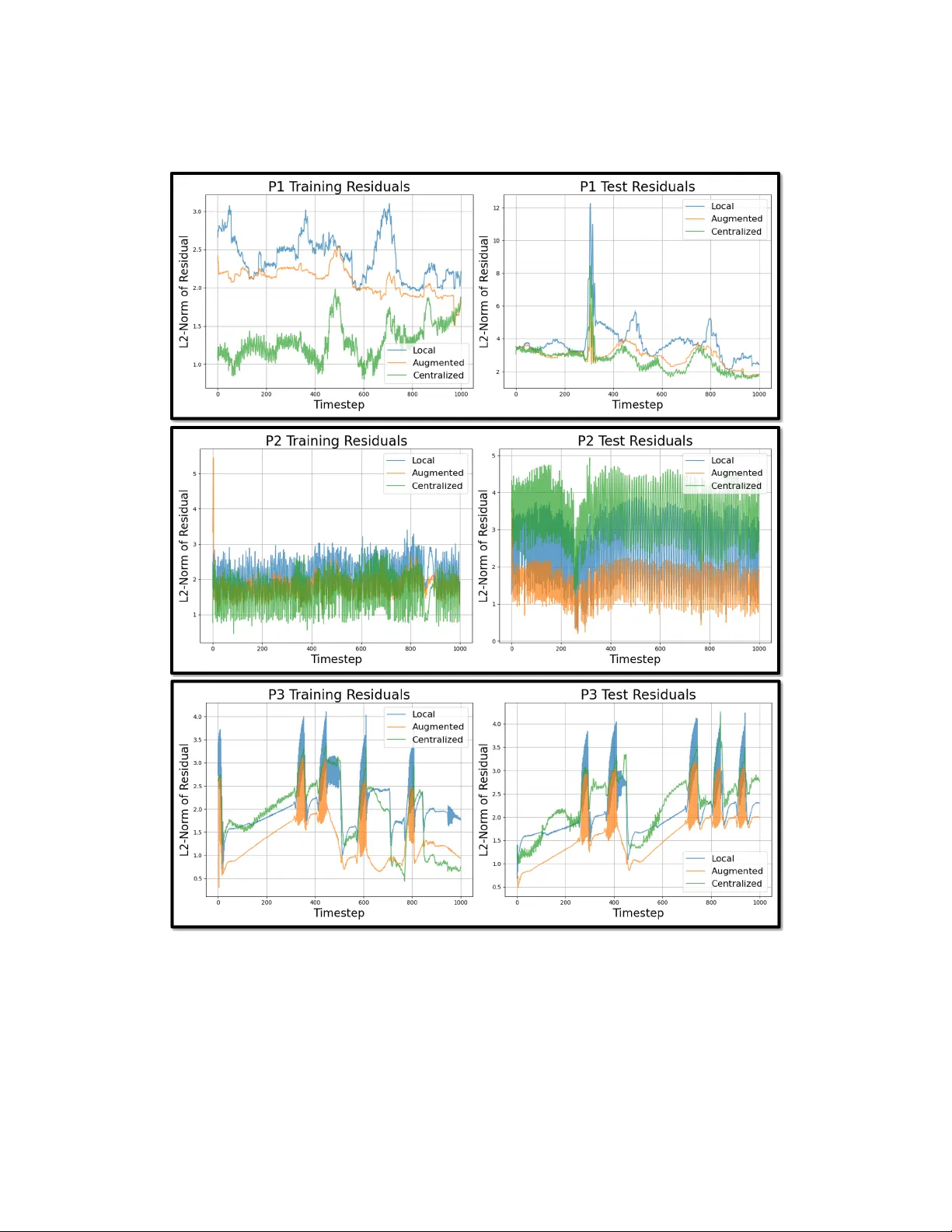
Loading comments...
Leave a Comment