Analyzing URA Geometry for Enhanced Near-Field Beamfocusing and Spatial Degrees of Freedom

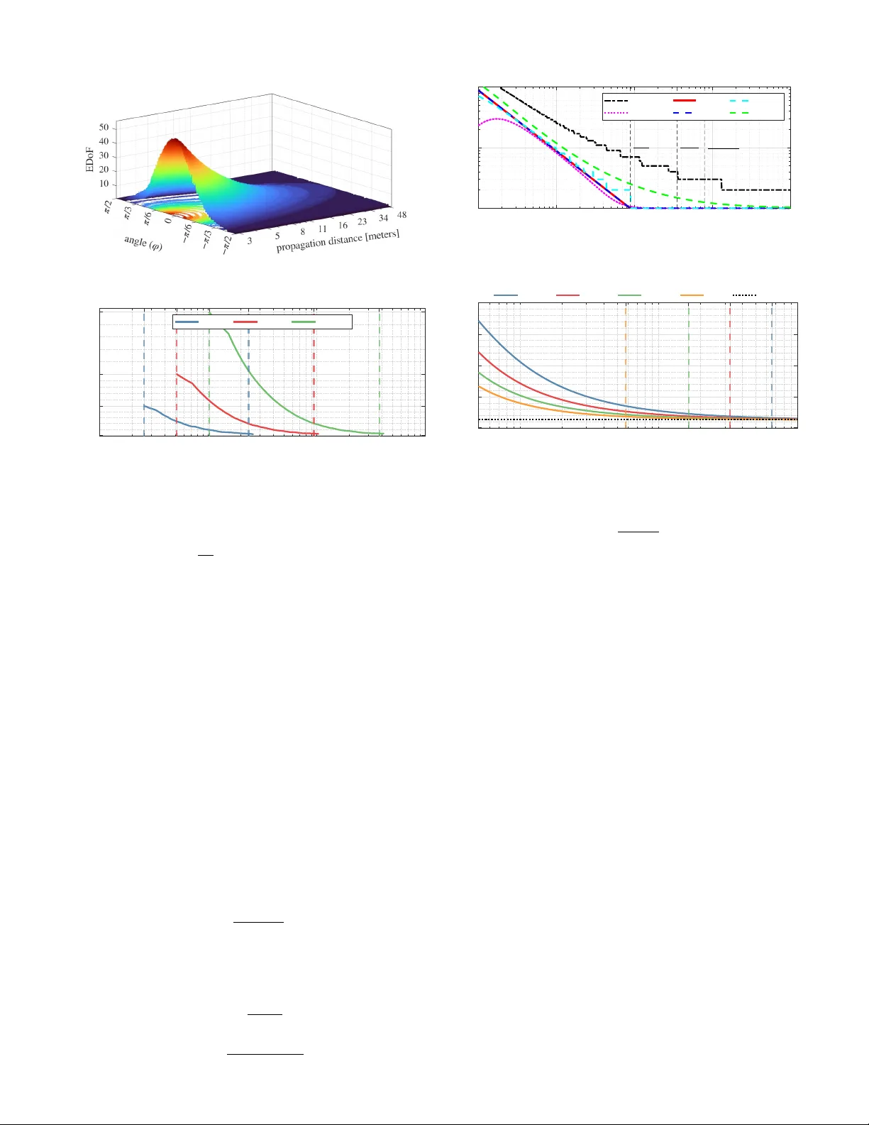
1 Analyzing URA Geometry for Enhanced Near -Field Beamfocusing and Spatial De grees of Freedom Ahmed Hussain, Asmaa Abdallah Senior Member , IEEE , Abdulkadir Celik, Senior Member , IEEE , Emil Björnson, F ellow , IEEE and Ahmed M. Eltawil, Senior Member , IEEE Abstract —With the deployment of large antenna arrays at high-frequency bands, future wireless communication systems are likely to operate in the radiative near -ﬁeld. Unlike far-ﬁeld beam steering, near-ﬁeld beams can be focused on a spatial region with a ﬁnite depth, enabling spatial multiplexing in the range dimension. Moreo ver , in the line-of-sight MIMO near -ﬁeld, multiple spatial degrees of freedom (DoF) are accessible, akin to a scattering- rich envir onment. In this paper , we derive the beamdepth for a generalized uniform rectangular array (URA) and investigate how the array geometry inﬂuences near-ﬁeld beamdepth and its limits. W e deﬁne the effective beamfocusing Rayleigh distance (EBRD), to present a near -ﬁeld boundary with respect to beamfocusing and spatial multiplexing gains for the generalized URA. Our results demonstrate that under a ﬁxed element count constraint, the array geometry has a strong impact on beamdepth, whereas this effect diminishes under a ﬁxed aperture length constraint. Moreov er , compared to uniform square arrays, elongated conﬁgurations such as unif orm linear arrays (ULAs) yield narro wer beamdepth and extend the effective near-ﬁeld region deﬁned by the EBRD. Building on these insights, we design a polar codebook for compressed-sensing-based channel estimation that leverages our ﬁndings. Simulation results show that the pr oposed polar codebook achieves a 2 dB NMSE improvement over state-of-the-art methods. Additionally , we present an analytical expression to quantify the effective spatial DoF in the near-ﬁeld, re vealing that they are also constrained by the EBRD. Notably , the maximum spatial DoF is achieved with a ULA conﬁguration, outperforming a square URA in this regard. Index T erms —Radiative near -ﬁeld, beamdepth, codebook, spa- tial degree of freedom, rectangular arrays, effective beamfocusing Rayleigh distance. I . I N T R O D U C T I O N M ASSIVE multiple-input multiple-output ( MIMO ) tech- nology is a cornerstone of ﬁfth generation ( 5G ) system advancements. Building on this foundation, future wireless networks are anticipated to lev erage ev en larger antenna arrays, such as ultra-massiv e ( UM )- MIMO , while progressing tow ard higher frequency spectra [ 2 ]. As carrier frequencies increase, the corresponding wav elengths decrease, enabling the deployment of larger antenna arrays within the given array size. The electromagnetic phenomenon surrounding an antenna array is typically divided into three regions: the reactiv e near- ﬁeld, the radiative near-ﬁeld, and the far-ﬁeld. In this work, we Ahmed Hussain, Asmaa Abdallah, Abdulkadir Celik, and Ahmed M. Eltawil are with Computer, Electrical, and Mathematical Sciences and Engineering (CEMSE) Division, King Abdullah University of Science and T echnology (KA UST), Thuwal, 23955-6900, KSA. Emil Björnson is with the School of Electrical Engineering and Computer Science, KTH Royal Institute of T echnology , 100 44 Stockholm, Sweden. The work of E. Björnson was supported by the Grant 2022-04222 from the Swedish Research Council. A conference version of this work is accepted in IEEE PIMRC 2025 [ 1 ]. refer to the radiativ e near-ﬁeld simply as the near-ﬁeld, which extends from the edge of the reactiv e zone out to the Rayleigh distance. W ithin this region, energy propagates with spherical wa vefronts and exhibits distance-dependent characteristics. Beyond the Rayleigh distance—which marks the boundary between the radiative near-ﬁeld and the far -ﬁeld—the curv ature of wa vefronts diminishes, allowing them to be approximated as planar wa ves with a phase error of less than π / 8 [ 3 ]. Qualcomm recently unv eiled a 4096-element Giga- MIMO prototype operating at 13 GHz , integrated within a form factor comparable to existing 256-element 5G base stations ( BS s) [ 4 ]. This advancement exempliﬁes a broader trend in future wireless systems: scaling up antenna arrays either by increasing the number of elements—enabled by higher carrier frequencies—or by expanding the physical aperture. Both approaches inherently enlarge the radiativ e near-ﬁeld region, making it a signiﬁcant portion of the communication region. Contemporary research underscores the potential of near-ﬁeld propagation to enhance both single-user and multiuser communication capacity [ 5 ]. In the near-ﬁeld regime, the ﬁnite beamdepth enables spatial separation of users located within the same angular direction, thereby improving multiuser capacity [ 6 ] for randomly located users. Simultaneously , the curvature of spherical wavefronts facilitates the transmission of multiple spatial data layers e ven under line-of-sight ( LoS ) conditions to a single multi-antenna device, thus augmenting single-user capacity [ 7 ]. Giv en the distance-dependent characteristics of near-ﬁeld propagation, this work aims to address three fundamental research questions. First, what are the spatial boundaries—speciﬁcally , the range limits across dif ferent angles—within which near-ﬁeld beamfo- cusing and multiple de grees of freedom ( DoF ) can be ef fectiv ely achiev ed? Outside these limits, the LoS channel exhibits far - ﬁeld behavior , characterized by inﬁnite beamdepth and a single spatial DoF . Second, how does the geometry of the antenna array inﬂuence beamdepth and the extent of the near-ﬁeld region, under practical constraints such as a ﬁxed aperture size or a ﬁxed number of antenna elements? Third, how do beam pattern characteristics in the range dimension compare to those in the angular dimension? By inv estigating these questions, this study seeks to deri ve ne w insights into how near-ﬁeld ef fects can be lev eraged to enhance spatial multiplexing, ultimately enabling high-capacity wireless communication systems. Furthermore, harnessing near-ﬁeld gains necessitates precise channel estimation, a challenge that becomes increasingly com- plex in UM - MIMO systems employing hybrid beamforming ( HBF ) [ 3 ]. While HBF signiﬁcantly reduces hardware costs and complexity by limiting the number of radio frequency ( RF ) 2 chains, it also constrains the number of observable in-phase and quadrature-phase ( IQ ) samples. As a result, achieving reliable channel estimates demands a higher pilot ov erhead, highlighting the need for efﬁcient estimation techniques along with polar codebook designs speciﬁcally tailored to near - ﬁeld conditions. While polar codebooks for uniform linear arrays ( ULA s) hav e been studied in [ 8 ], [ 9 ], practical systems predominantly employ uniform rectangular arrays ( URA s), which accommodate a lar ger number of antenna elements within a constrained physical area. The polar codebooks de veloped for ULA s are not directly applicable to URA s due to their complex array gain functions. Moreo ver , the analysis and design of URA - based polar codebooks is challenging because of the coupling among azimuth, ele vation, and range parameters. A. Related W ork Foundational work on near-ﬁeld beamforming [ 10 ] deriv ed beamdepth expressions for square aperture antennas, later extended to planar arrays in [ 11 ]. Notably , the beamdepth analyses in [ 10 ], [ 11 ] are based on continuous aperture ( CAP ) antennas, where the Rayleigh distance of the array is deﬁned as the product of the number of antenna elements and the Rayleigh distance of the individual antenna element. In contrast, we deﬁne the Rayleigh distance of the array as r RD = 2 D 2 λ , where D represents the aperture length of the antenna array . Furthermore, explicit closed-form beamdepth expressions in [ 10 ], [ 11 ] are limited to boresight transmissions, underscoring the need for angle-dependent beamdepth analysis for spatially discrete (SPD) antennas. The capacity of a MIMO system grows linearly with the spatial DoF , which are inﬂuenced by both the scattering en vironment and the array geometry [ 12 ]. For large CAP antennas, the spatial DoF are fundamentally bounded by 2 λ per meter for a linear segment and π λ 2 per square meter for planar segments [ 13 ]. The maximum spatial DoF is limited by the number of antenna elements and is the same in both near and far-ﬁeld [ 7 ]. Maximum spatial DoF in the LoS far -ﬁeld channel equals one; howe ver , spherical wavefronts in the near- ﬁeld enable access to enhanced spatial DoF . Given a constraint on a ﬁxed number of antenna elements, we aim to determine the angle-dependent limit within the near-ﬁeld where the spatial DoF exceeds one for different array geometries. Recent studies have indicated that the classical Rayleigh distance often overestimates the extent of the effecti ve near- ﬁeld region [ 14 ], prompting the de velopment of alternative metrics to more accurately characterize near-ﬁeld ef fects and predict when they can be utilized to achie ve more well- conditioned channels. T o model a wideband near -ﬁeld channel, [ 15 ] introduced the concept of effecti ve Rayleigh distance ( ERD ), based on far-ﬁeld beamforming loss in the near-ﬁeld region, and this idea was expanded to wideband phased arrays with the bandwidth-aware near -ﬁeld distance ( B AND ) [ 16 ]. The ERD and the B AND cov er only a small fraction of the near -ﬁeld region, as deﬁned by the Rayleigh distance. Howe ver , these metrics are based on far -ﬁeld beamforming loss and therefore do not adequately capture near-ﬁeld effects. The effecti ve beamfocusing Rayleigh distance ( EBRD ) metric was proposed in [ 8 ] to characterize the limits of polar-domain sparsity for ULA s. Despite these advancements, an angle-dependent spatial limit for URA s—one that jointly characterizes beamfocusing and spatial DoF—remains undetermined. Near-ﬁeld beamfocusing requires geometry-dependent phase compensation to account for spherical wav efront curvature. In particular, the achie vable beamdepth is governed by the effecti ve aperture length, which is determined by the diagonal (i.e., the maximum dimension) of the URA . In this context, further research is needed to in vestigate array geometries that enable narro w beamdepth and extended near-ﬁeld boundaries, to guide the design of future networks that enable more users to beneﬁt from near -ﬁeld propagation. This paper addresses these gaps by exploring the interplay of array geometry and near-ﬁeld electromagnetic properties. Herein, we present a comprehensive analysis of the near-ﬁeld beam pattern, examining key metrics such as beamdepth, limits of the beamdepth, beam resolution, spatial DoF , and the inﬂuence of array geometry on these parameters. In contrast to [ 11 ], we derive angle-dependent expressions for near-ﬁeld beamfocusing. Moreover , we exploit this characterization to design polar codebooks for near-ﬁeld channel estimation. B. Contribution This work explores near -ﬁeld beamfocusing for an SPD URA with a generic width-to-height ratio. W e derive the normalized array gain using Fresnel functions, based on which we formulate a beamdepth expression. Additionally , we establish angle-dependent limits for beamfocusing and characterize the near-ﬁeld beam pattern in terms of resolu- tion and sidelobe lev els across both the range and angular dimensions. Furthermore, we examine the inﬂuence of spatial focus regions and array geometry on near-ﬁeld beamdepth. Drawing inspiration from the far-ﬁeld codebook in the angular domain—where beams spaced by the 3 dB angular beamwidth hav e minimum correlation while maximizing the cov erage—we propose constructing a polar codebook where code words are separated by the beamdepth in the distance dimension. W e also characterize the near-ﬁeld spatial DoF using a Fresnel-based gain function and in vestigate ho w the array geometry af fects these spatial DoF . The main contributions of this paper are summarized belo w: • Beamdepth and effective beamfocusing Rayleigh dis- tance: W e derive a closed-form beamdepth and EBRD expression for a URA , establishing the maximum angle- dependent range limit for ﬁnite-depth beams. Our anal- ysis demonstrates how array geometry inﬂuences both beamdepth and EBRD , providing critical insights for enhancing multiuser capacity in near-ﬁeld communication. • Characterization of near-ﬁeld beam pattern: W e com- pare and contrast near-ﬁeld beam patterns across range and angle dimensions with respect to beam resolution and sidelobe levels. Furthermore, we propose a window function that attenuates sidelobes in the range dimension. • Spatial degrees of fr eedom: W e derive a Fresnel- based gain function to characterize the effecti ve degrees of freedom ( EDoF ) across dif ferent array geometries. 3 Furthermore, we analyze the boundary beyond which the EDoF in the near -ﬁeld and far-ﬁeld become equiv alent. • Polar codebook design: Lev eraging the near-ﬁeld beam- forming and beam pattern analysis, we propose a novel polar codebook tailored for near-ﬁeld channel estimation in a URA . The proposed codebook enhances channel estimation performance by constructing codewords with low column coherence while improving computational efﬁcienc y through a reduced codebook size. C. Notations and Organization of the P aper Matrices, vectors, and scalars are denoted by bold uppercase, bold lowercase, and lowercase letters, respectively . The expecta- tion, transpose, and conjugate transpose operations are denoted by E [ · ] , ( · ) T , and ( · ) H respectiv ely . The uniform distribution between a and b is annotated by U ( a, b ) . Furthermore, ⊙ represents the Hadamard product. The remainder of the paper is structured as follo ws. Section II presents the near-ﬁeld channel model, followed by Section III , which deri ves the beamdepth and the EBRD. Section IV ana- lyzes the near-ﬁeld beam pattern, and Section V characterizes the spatial DoF . The design of the polar codebook is detailed in Section VI , and conclusions are drawn in Section VII . I I . S Y S T E M M O D E L W e consider a narrow-band communication system equipped with a UM scale antenna array at the BS and a single isotropic antenna user equipment ( UE ) as depicted in Fig. 1 . The antenna array consists of a URA with N BS small antennas, arranged with N 1 elements along the y-axis and N 2 elements along the z-axis, respecti vely . The element spacing along both axes is the same and equals d y = d z = d = λ 2 . Antenna elements along the y-axis are indexed as n 1 ∈ [ − ∼ N 1 , · · · , 0 , · · · , ∼ N 1 − 1] where ∼ N 1 = N 1 2 . Likewise, the antenna elements along z-axis are index ed as n 2 ∈ [ − ∼ N 2 , · · · , 0 , · · · , ∼ N 2 − 1] where ∼ N 2 = N 2 2 . The aperture length of the URA can be determined from the Pythagorean theorem as D = d p N 2 1 + N 2 2 . The aspect ratio of the array is deﬁned as η = N 1 N 2 . When η > 1 , the array exhibits a wide conﬁguration, whereas η < 1 corresponds to a tall conﬁguration. In the extreme cases where η ≫ 1 or η ≪ 1 , the URA approaches a ULA . In particular , a ULA is obtained when its physical length equals the aperture length D . The UE subtends azimuth angle φ , ele vation angle θ , and is positioned at a distance r from the BS . In this paper , the minimum distance in the radiativ e near-ﬁeld is set as 2 D such that amplitude variations across the array are negligible, and accordingly , a uniform spherical wa ve ( USW ) model is employed [ 17 ]. The normalized near-ﬁeld array response vector for a ULA with N 1 antenna elements is expressed as b ULA ( φ, r ) = 1 √ N 1 h e − j ν ( r ( − ∼ N 1 ) − r ) , . . . , e − j ν ( r ( ∼ N 1 ) − r ) i , (1) where ν = 2 π f c c is the wav enumber, with f c as the carrier frequency and r ( n ) is the distance between the UE and the n th antenna element of the ULA . For a URA with N BS = N 1 N 2 y - axis UE (− 𝑁 " ! , 𝑁 " " −1 ) z - axis 𝜃 𝜑 x - axis 𝑟 𝑁 " 𝑑 # 𝐷 𝑑 $ 𝑑 # 𝑁 ! 𝑑 $ ( 𝑁 " ! −1 , 𝑁 " " −1 ) (− 𝑁 " ! , - 𝑁 " " ) ( 𝑛 ! , 𝑛 " ) 𝑟 (& ! , & " ) Fig. 1: URA setup and a single prospectiv e user . elements, the near-ﬁeld array response vector b URA ( φ, θ , r ) can be obtained based on the spherical-wa ve propagation model as b URA ( φ, θ , r ) = 1 √ N BS  e − j ν  r ( − ˜ ζ ) − r  , · · · , e − j ν  r ( ˜ ζ ) − r   , (2) where e ζ = ( ∼ N 1 , ∼ N 2 ) . The distance r ( n 1 ,n 2 ) between the UE and ( n 1 , n 2 ) th element of the URA is given by r ( n 1 ,n 2 ) = q ( r u x − 0) 2 + ( ru y − n 1 d ) 2 + ( ru z − n 2 d ) 2 , ( a ) ≈ r − n 1 du y − n 2 du z + n 2 1 d 2 2 r β 1 · · · + n 2 2 d 2 2 r β 2 − n 1 n 2 d 2 u y u z r , ( b ) ≈ r − n 1 du y − n 2 du z + n 2 1 d 2 2 r β 1 + n 2 2 d 2 2 r β 2 , (3) where the directional cosines are u x = sin θ cos φ , u y = sin θ sin φ , and u z = cos θ . Approximation (a), also termed the near-ﬁeld expansion , is derived from the second-order T aylor expansion √ 1 + x ≈ 1 + x 2 − 1 8 x 2 , that is tight for small v alues of x . Furthermore, β 1 = 1 − sin 2 θ sin 2 φ and, β 2 = 1 − cos 2 θ . T o make the following analysis tractable, we omit the last term in ( 3 ) (a) to obtain ( 3 ) (b), as it is negligible for large v alues of N BS [ 18 ], and accounts for only 5% of the array gain [ 5 ]. Furthermore, when r is greater than the Rayleigh distance r RD = 2 D 2 λ , the terms in volving 1 r can be ignored, and ( 2 ) degenerates to the far-ﬁeld steering vector a URA ( φ, θ ) = 1 √ N BS " e − j ν d  − ∼ N 1 sin φ sin θ − ∼ N 2 cos θ  , · · · , 1 , · · · , e − j ν d  ∼ N 1 sin φ sin θ + ∼ N 2 cos θ  # ∈ C N 1 N 2 × 1 . (4) I I I . A N A LY S I S O F N E A R - FI E L D B E A M F O R M I N G Finite-depth beamforming is achiev able in the radiativ e near- ﬁeld through the conjugate phase method. In this approach, the phase of each antenna element is adjusted to compensate for the path-length difference between the focal point and the antenna element, thereby ensuring constructiv e interference at the focal point. The resulting beam, as depicted in Fig. 4 𝜃 !" 𝜑 !" 𝑟 # $%& 𝑟 # $'( 𝑟 !" # = 𝑟 $ %&' − 𝑟 $ %() ∆ 𝑟 %) ∆ 𝑟 *+ 𝑟 # 𝑟 $ − 𝑟 $ %() $ < $ 𝑟 $ %&' − 𝑟 $ Fig. 2: Near-ﬁeld beam with ﬁnite beamdepth and beamwidth in the axial and lateral dimensions, respectively . 2 , has an azimuth beamwidth φ BW , elev ation beamwidth θ BW and beamdepth r BD . In this section, we deriv e the beamdepth and the maximum range limits within which the ﬁnite depth beamforming can be achie ved, referred to as the EBRD for a URA . W e inv estigate how the spatial focus region and array geometry inﬂuence the v ariation in beamdepth and the extent of the EBRD. W e assume a LoS channel between the UE and the BS . The near-ﬁeld channel h ∈ C N BS × 1 based on the USW model is mathematically formulated as [ 19 ] h = √ g b ( φ, θ , r ) , (5) where g denotes the channel gain taking into account the path loss and antenna gain, and r is the distance between the UE and the origin of the URA . W e consider a BS equipped with a generalized URA that serves a near-ﬁeld UE located at ( φ, θ , r F ) . Let w ( φ, θ , z ) denote the beamforming vector based on the conjugate phase method. The array gain G URA characterizes the normalized receiv ed po wer, and is deﬁned as G URA =    w ( φ, θ , z ) H h ( φ, θ , r F )    2 , ∀ φ ∈ [ − π / 2 , π / 2] , θ ∈ [ − π / 2 , π / 2] , z ∈ [2 D , ∞ ] . (6) In the subsequent analysis, we utilize ( 6 ) to deri ve array gain for the URA and characterize beamdepth and EBRD for different array geometries. A. Finite Beamdepth and EBRD W e deﬁne the beamdepth, r BD , as the distance interval z ∈ [ r min F , r max F ] where the normalized array gain is at most 3 dB belo w its maximum value. The beamforming vector w ( φ, θ , z ) in ( 6 ), designed using conjugate phase, achie ves maximum array gain at the focal point z = r F and decreasing array gain at distances aw ay from r F . Then the normalized array gain in ( 6 ) achie ved by w ( φ, θ , z ) is giv en by G URA ≈      1 N 1 N 2 X n 1 X n 2 e j π λ ( n 2 1 d 2 β 1 + n 2 2 d 2 β 2 ) z eff      2 , (7) where z eﬀ =    z − r F z r F    . Since N BS is large, the summation in ( 7 ) can be approximated with a Riemann integral 1 to obtain G URA ≈       1 N 1 N 2 Z N 1 2 − N 1 2 Z N 2 2 − N 2 2 e j π λ ( n 2 1 d 2 β 1 + n 2 2 d 2 β 2 ) z eff d n 1 d n 2       2 . (8) By the change of v ariables x 1 = q 2 n 2 1 d 2 β 1 z eff λ and x 2 = q 2 n 2 2 d 2 β 2 z eff λ , we express the array gain in ( 8 ) in terms of Fresnel functions as G URA =  C 2 ( γ 1 ) + S 2 ( γ 1 )   C 2 ( γ 2 ) + S 2 ( γ 2 )  ( γ 1 γ 2 ) 2 , (9) where C ( γ i ) = R γ i 0 cos  π 2 x 2 i  dx i and S ( γ i ) = R γ i 0 sin  π 2 x 2 i  dx i are the Fresnel functions [ 6 ], with i ∈ { 1 , 2 } . Moreov er, γ 1 = q N 2 1 d 2 β 1 2 λ z eﬀ and γ 2 = q N 2 2 d 2 β 2 2 λ z eﬀ . Based on the gain function in ( 9 ) , we present Theorems 1 and 2 to characterize the 3 dB beamdepth and the EBRD, respectiv ely . Theorem 1. For a generalized URA , the 3 dB beamdepth r BD obtained by focusing a beam at a distance r F from the BS is giv en by r BD = 8 r 2 F r RD α 3dB η ( η 2 + 1) √ β 1 β 2  η r RD √ β 1 β 2  2 − [4 α 3dB r F ( η 2 + 1)] 2 . (10) Pr oof. Proof is provided in Appendix A . Theorem 2. The farthest distance for a giv en pair of azimuth and ele vation angles, at which near-ﬁeld beamfocusing for a URA can be achiev ed, is termed the effecti ve beamfocusing Rayleigh distance r EBRD and is gi ven by r F < η r RD 4 α 3dB (1 + η 2 ) sin θ q 1 − sin 2 θ sin 2 φ. (11) Pr oof. Proof is provided in Appendix B . The beamdepth and EBRD expressions for a uniform square array (USA) and a ULA can be derived as follows: Corollary 1. For a USA , beamdepth r USA BD is obtained by substituting η = 1 in ( 10 ) to get r USA BD = ( 16 r 2 F r RD α 3dB √ β 1 β 2 ( r RD √ β 1 β 2 ) 2 − (8 α 3dB r F ) 2 , r F < r RD 8 α 3dB √ β 1 β 2 , ∞ , r F ≥ r RD 8 α 3dB √ β 1 β 2 . (12) Note that in the boresight case √ β 1 β 2 = 1 and α 3dB = 1 . 25 , ( 12 ) reduces to the beamdepth expression in [Eq. 23, [ 10 ]]. The boresight case of a URA was considered in [ 11 ]. Corollary 2. For a ULA along y-axis, beamdepth r ULA BD is giv en by r ULA BD = ( 8 α 3dB r 2 F r RD cos 2 ( φ ) ( r RD cos 2 ( φ )) 2 − (4 α 3dB r F ) 2 , r F < r RD 4 α 3dB cos 2 ( φ ) , ∞ , r F ≥ r RD 4 α 3dB cos 2 ( φ ) . (13) The special case of a ULA was cov ered in [ 3 ]. Beamdepth for uniform circular array (UCA) is derived in [ 20 ]. 1 For large N BS with small antenna elements, the discrete sum conv erges to the Riemann integral. 5 W e ev aluate the impact of the approximation in ( 3 ) (b), where the cross term is neglected, on the beamdepth expression in ( 10 ) by comparing it with the numerically computed beamdepth. The numerical beamdepth is obtained by computing the array gain using the exact array response vector in ( 2 ) and identifying the 3 dB points of the resulting gain function. As shown in Fig. 3 , the analytical beamdepth closely matches the numerical results, with a slight deviation observed at very short focal distances ( < 2 D ). At larger distances, this deviation vanishes as the contribution of the neglected cross term diminishes. Moreover , since the EBRD represents the maximum distance limit for beamfocusing, the approximation in ( 3 ) (b) has a negligible impact on the EBRD . Note that the EBRD is conceptually distinct from the ERD in [ 15 ]. Speciﬁcally , the ERD deﬁnes the boundary at which the beamforming loss incurred when approximating the near-ﬁeld channel with a far -ﬁeld model exceeds a prescribed threshold. For a ULA , the ERD is giv en by 0 . 367 r RD cos 2 ( φ ) for a threshold of 0 . 05 . As shown in Fig. 4 , the ERD ov erestimates the near-ﬁeld region from a beamfocusing perspecti ve, whereas only the region within the EBRD truly supports beamfocusing. B. Impact of Spatial F ocus Region and Array Geometry A narro wer beamdepth in the near-ﬁeld allows for serving more users within the same angular direction while reducing mutual interference. In the following, we analyze how both beamdepth and EBRD vary with spatial focus region and array geometry . 1) Spatial F ocus Re gion: In the far -ﬁeld, the beamwidth broadens as the beam is steered aw ay from the boresight [Fig. 1, [ 2 ]]. Similarly , the beamdepth r BD increases as the focal region moves farther away from the array , as indicated by the quadratic dependence on r F in ( 10 ) . This can also be observed from the approximate expression in ( 16 ) (Section IV -A 1 ) and from Fig. 16 (Section VI ). In the principal plane 2 , beamdepth is minimal at the boresight and expands tow ard the endﬁre directions. For wide arrays ( η ≫ 1 ), beamdepth is primarily inﬂuenced by the azimuth angle φ , whereas for taller arrays ( η ≪ 1 ), it is mainly gov erned by the ele vation angle θ . In the cross plane, the v ariation of the beamdepth is more complex as both the length and width of the aperture affect it. T o exemplify , the variation of beamdepth with respect to the azimuth angle φ for different URA conﬁgurations is shown in Fig. 5 , where r BD increases at larger azimuth angles for wide arrays. Likewise, as the ele vation angle θ increases from the boresight π / 2 to endﬁre direction 5 π / 6 , beamdepth r BD increases signiﬁcantly for tall arrays. Ho wever , in the cross plane, beamdepth decreases at large elev ation angles for wide arrays. A similar trend for beamwidth in the angular domain is reported in [Fig. 2.16, [ 21 ]]. 2) Array Geometry: For a ﬁxed number of antenna elements N BS = N 1 N 2 , different array geometries can be realized by v arying the aspect ratio η = N 1 / N 2 , which results in dif ferent aperture lengths given by D = d p N 2 1 + N 2 2 . Alternati vely , one can ﬁx the aperture length D and v ary η , allo wing N BS to 2 For wide arrays, azimuth is considered the principal plane, whereas for tall arrays, elevation serves as the principal plane. 0 20 40 60 80 100 120 140 fo c us di sta nc e [m ete rs ] 10 ! 2 10 0 10 2 b ea m dep th [ me te rs] Approximate (10) Numerical 1 2 3 10 ! 2 10 ! 1 Fig. 3: Numerical and analytical beamdepth for a (256 × 16) URA operating at 30 GHz . The zoom inset highlights the beamdepth for focus distances less than 2 D = 5 . azimuth ang le ( ' ) ! : = 2 ! : = 4 0 : = 4 : = 2 dis tance [ mete rs] 0 100 200 300 400 Beamfocusing Rayleigh distance ERD EBRD Fig. 4: Near-ﬁeld boundary in terms of ERD and EBRD for a ULA . Here f c = 28 GHz , N BS = 256 , r RD = 348 m . scale with the array shape. Furthermore, by keeping D constant and v arying the operating frequency , N BS can be adjusted as a function of both array geometry and wavelength. In the follo wing analysis, we examine all three scenarios. T o provide analytical insights, the beamdepth expression in ( 10 ) can be approximated for boresight transmission as r BD ≈ 8 r 2 F α 3dB ( η 2 + 1) η r RD , (14) where r F remains the same for all the array conﬁgurations. (i) F ixed Number of Antenna Elements: For a ﬁx ed number of elements N BS = N 1 N 2 , the aperture length D = d p N 2 1 + N 2 2 is minimized when the array is square, i.e., N 1 = N 2 , corresponding to a USA . As a result, the Rayleigh distance r RD = 2 D 2 λ is minimized for square arrays and maximized for ULA conﬁgurations. Additionally , the combined term α 3dB  η 2 +1 η  achiev es its maximum v alue when η = 1 , i.e., for a square URA, and diminishes for other aspect ratios. Therefore, beamdepth r BD is maximized when the array is square, as sho wn in Fig. 6 (black curve). (ii) F ixed Apertur e Length: For a ﬁxed aperture length D , the Rayleigh distance r RD remains constant across different aspect ratios. Ho wever , the composite factor α 3dB  η 2 +1 η  , which directly inﬂuences beamdepth, reaches its maximum for a square array . Howe ver , as shown in Fig. 6 (blue curve), the variation of beamdepth with respect to η is less signiﬁcant under a ﬁxed aperture length than in the ﬁxed element count scenario. This is because r RD —being relati vely large in magnitude—dominates the beamdepth expression ( 14 ) , making the inﬂuence of the geometry-dependent factor α 3dB  η 2 +1 η  comparativ ely minor . Extending the Giga- MIMO example discussed in Section I , 6 ! : = 3 ! : = 6 0 : = 6 : = 3 azimuth an gle ( ' ) 10 ! 2 10 ! 1 10 0 10 1 10 2 b eam depth [me ters] Wide URA , 128x32 Wide URA , 256x16 T all URA , 4x1024 T all URA , 2x2048 2 =4 2 =16 2 =1/256 2 =1/1024 3 = : = 2 3 = 2 : = 3 3 = 5 : = 6 Fig. 5: Beamdepth with respect to azimuth angle φ for different array conﬁguration η and elevation angle θ . 2 ! 6 2 ! 4 2 ! 2 2 0 2 2 2 4 2 6 arra y con - guration ( 2 ) 10 0 10 1 b eamdepth [meters] N BS = 4096 ; f c = 15GHz D = 1 m, f c =15 GHz D = 1 m, f c =30 GHz D = 1 m, f c =60 GHz Fig. 6: Beamdepth with respect to η for ﬁxed number of antenna elements N BS and aperture length D . we further analyze the impact of the operating frequency on the beamdepth under a ﬁxed aperture length D . Fig. 6 presents the simulated beamdepth behavior for D = 1 m when the carrier frequenc y increases from 15 GHz to 60 GHz . The results demonstrate a clear decrease in beamdepth with increasing frequency . This trend is consistent with the approximation in ( 14 ) , where the Rayleigh distance r RD increases with frequency (due to the corresponding decrease in wavelength), thereby reducing the beamdepth e ven for a ﬁxed aperture length. 3) Limits of Beamfocusing: The EBRD deﬁnes the near- ﬁeld boundary beyond which beamfocusing becomes infeasible. W ithin the EBRD boundary , beamfocusing enables serving multiple users in the same angular direction, thereby enhancing multiuser capacity . It is therefore important to in vestigate methods for enlarging the EBRD . W e ﬁrst analyze the case with a ﬁxed element count, followed by the case with a ﬁxed aperture length. (i) F ixed Number of Antenna Elements: Based on ( 11 ) , since the Rayleigh distance r RD is minimal for a square URA , and it dominates the other factor as explained earlier , the EBRD is smallest for square URA and increases as the URA geometry transitions toward a ULA . This relationship is illustrated in Fig. 7 , where the EBRD is plotted with respect to azimuth angle φ , and as a function of η and elev ation angle θ . Additionally , the EBRD for wide arrays varies with the azimuth angle, while for tall arrays, it depends on the elev ation angle. For all conﬁgurations in the principal plane, the EBRD reaches its maximum at the boresight direction ( φ = 0 , θ = π / 2 ) and decreases in the endﬁre directions. The largest EBRD is observed for the URA conﬁguration with η = 0 . 004 , while the smallest EBRD is associated with the square URA conﬁguration ( η = 1 ). Note that the EBRD for η = 0 . 016 and η = 0 . 004 remains constant with respect to the azimuth angle φ , as these conﬁgurations represent tall URA s ( η ≪ 1 ). Furthermore, for these tall arrays, the EBRD decreases further when the elev ation angle deviates from the boresight ( θ = π / 2 ). (ii) F ixed Apertur e Length: For a ﬁxed aperture length, the square array continues to exhibit the lowest EBRD , while the variation in EBRD across dif ferent array geometries becomes less pronounced—consistent with the beamdepth behavior discussed earlier . Building on this, we now ﬁx the array geometry and in vestigate how the EBRD scales with aperture length D and operating frequency . The objective is to identify the dominant factor that driv es the expansion of the EBRD region, thereby identifying the array geometries enabling more users to beneﬁt from near -ﬁeld communication. T o this end, we e valuate EBRD as a function of azimuth angle for varying aperture sizes and carrier frequencies as shown in Fig. 8 . At D = 1 m—which approximates the physical dimensions of the Giga- MIMO array— EBRD at boresight reaches approximately 13 m at 15 GHz. Increasing the frequency to 60 GHz extends the EBRD to around 55 m, though this increase may still be modest. In contrast, increasing the aperture length offers a more signiﬁcant impact: as shown in Fig. 8 , the EBRD reaches approximately 123 m at 15 GHz when D is increased to 3 m. This dominant effect of aperture size ov er frequency can be attributed to the scaling behavior of the Rayleigh distance r RD = 2 D 2 λ , which increases quadratically with D but only linearly with wav elength. Thus, enlarging the aperture length seems to be a more effecti ve strategy for substantially expanding the near-ﬁeld region. C. Multiuser Capacity Analysis In this subsection, we present numerical examples to ev aluate multiuser capacity with respect to the EBRD and the array geometry . W e consider a hybrid beamformer with analog precoder W . Additionally , zero-forcing is applied as the digital precoder . The overall spectral efﬁciency (SE) is giv en by R = 5 X m =1 log 2 1 + p m   h H m Wf m   2 σ 2 m + P l  = m p l | h H m Wf l | 2 ! , (15) where p m denotes power allocated to the m th user and σ 2 m denotes the noise variance. Furthermore, f m represents the m th column of the digital precoder . 1) SE vs. EBRD: Finite beamdepth is achiev able only within the EBRD region, limiting spatial multiplexing gains due to beamdepth to the near-ﬁeld region bounded by the EBRD . T o illustrate this, we consider a 64 × 8 URA serving ﬁv e users positioned in the boresight direction ( φ = 0 , θ = π / 2) . Users are distributed uniformly across three distinct regions: the EBRD region [2 D , r EBRD ] , the near-ﬁeld region beyond EBRD [ r EBRD , r RD ] , and the far-ﬁeld region [ r RD , 100 r RD ] . W e employ both polar and discrete Fourier transform ( DFT ) codebooks for each of these scenarios. The resulting SE is shown in Fig. 9 . W ithin the EBRD region, the polar codebook achiev es a SE of 5 . 8 bps/Hz, compared to only 2 bps/Hz with the DFT codebook. Additionally , SE is similar for both codebooks in 7 10 1 10 2 10 3 10 4 EB RD [me ter s] ! : = 3 ! : = 6 0 : = 6 : = 3 azi mu th a ngl e ( ' ) USA 64x64 Wide URA 128x32 Wide URA 256x16 T all URA 8x512 ULA 4x1024 2 =1 2 =4 2 =16 2 =.016 2 =.004 3 = : = 2 3 = 2 : = 3 3 = 5 : = 6 Fig. 7: Finite beamdepth limit in terms of EBRD with respect to azimuth angle for different array conﬁgurations and elev ation angles. 10 0 10 1 10 2 10 3 EB RD [me ter s] ! : = 3 ! : = 6 0 : = 6 : = 3 azi mu th a ngl e ( ' ) 13 27 55 123 247 497 344 687 1370 D = 1 m D = 3 m D = 5 m f c = 15 GHz f c = 30 GHz f c = 60 GHz Fig. 8: Finite beamdepth limit in terms of EBRD with respect to azimuth angle for different aperture lengths and frequencies. the near-ﬁeld region outside the EBRD and in the far-ﬁeld. It is important to emphasize that the EBRD determines the near-ﬁeld boundary in terms of multiplexing gain when UE s are distributed linearly along a single angular direction in the range domain. For uniformly distrib uted UE s, regions outside the EBRD may still achiev e slightly higher SE than the far - ﬁeld case, o wing to the improved lateral resolution at shorter distances compared to the far -ﬁeld. 2) SE vs. Array Geometry: Array geometry governs both beamdepth and the EBRD ; howe ver , its impact diminishes under a ﬁxed aperture length constraint. Nonetheless, under both ﬁxed-element and ﬁxed-aperture scenarios, elongated array conﬁgurations like ULA yield the smallest beamdepth and the largest EBRD, thereby enhancing spatial multiplexing. T o quantify the impact of array geometry , we ev aluate the SE , as depicted in Fig. 10 , across η = [1 , 4 , 16] , under two constraints: ﬁxed aperture length D and ﬁxed number of elements N BS . As a baseline, the square URA conﬁguration ( η = 1 ) is used, which is expected to yield the lowest SE due to its wider beamdepth and limited EBRD . In all scenarios, ﬁv e users are randomly distributed along the boresight direction within the range [2 D , r EBRD ] , where r EBRD varies with array geometry . Under the ﬁxed-element constraint ( N BS = 1024 ), SE increases consistently with η , i.e., from η = 1 to η = 16 , across all signal-to-noise ratio ( SNR ) v alues. This trend aligns with Fig. 6 (black curve), where a reduction in beamdepth with increasing η (i.e., transitioning to ward a ULA ) mitigates inter-user interference and enhances SE. Under the ﬁxed-aperture constraint ( D = 2 ), the SE trend is more interesting. While the conﬁguration with η = 4 achiev es SN R [ dB ] 5 7 9 11 13 15 17 19 21 23 25 27 29 SE [bp s/H z] 0 2 4 6 8 10 Polar co debo ok U [2 D; r EB RD ] DFT codeb ook U [2 D; r EB RD ] Polar co debo ok U [ r EB RD ; r RD ] DFT codeb ook U [ r EB RD ; r RD ] Polar co debo ok U [ r RD ; 100 r RD ] DFT codeb ook U [ r RD ; 100 r RD ] Fig. 9: The comparison of SE versus SNR, with respect to user distribution. SN R [ dB ] 5 7 9 11 13 15 17 19 21 23 25 27 29 SE [bp s/H z] 2 4 6 8 10 2 = 16, N B S = 1024 2 = 4, N B S = 1024 2 = 4, D = 2 m 2 = 16, D = 2 m 2 = 1, ( N B S = 1024 ; D = 2 m ) Fig. 10: The comparison of SE versus SNR, with respect to array conﬁgurations. higher SE than η = 1 , the SE for η = 16 drops compared to η = 4 . This behavior can be explained by the SE expression in ( 15 ) , where the numerator is inﬂuenced by the beamforming gain, dependent on the number of antenna elements, and the denominator reﬂects mutual interference. Since beamdepths for η = 4 and η = 16 are nearly identical (as shown in Fig. 6 ), the v ariation in SE arises primarily from the reduced element count in the η = 16 conﬁguration, which diminishes the beamforming gain and thereby reduces the overall SE. I V . A X I A L V S . L AT E R A L B E A M P AT T E R N A N A LY S I S Beam resolution is key to maximizing wireless commu- nication capacity by enabling precise user separation and minimizing interference. In the near -ﬁeld, beams can be focused in both the axial (range) and lateral (angular) dimensions, making it instructi ve to analyze and compare beam patterns in these dimensions. In the subsequent analysis, we examine the beam resolution, as well as the sidelobe patterns, in both the axial and lateral dimensions to provide a comparative analysis and implications for near -ﬁeld wireless communication. A. Beam Resolution Axial and lateral resolution are determined by the beamdepth and beamwidth, respectiv ely . For tractability , we compare beamdepth and beamwidth of a ULA at a ﬁxed distance r F . Speciﬁcally , we consider a ULA with boresight transmission, where α 3dB = 1 . 75 for φ = 0 ◦ . 8 1) Axial Resolution: For this conﬁguration, the denominator in ( 13 ) is simpliﬁed to ( r 2 RD − 49 r 2 F ) . A ﬁnite value of r ULA BD is attained only when r F < r RD 7 , ensuring that r 2 RD remains signiﬁcantly larger than 49 r 2 F . Consequently , we can neglect the 49 r 2 F term and substitute r RD = 2 D 2 λ in ( 13 ) , yielding the following simpliﬁed expression for beamdepth of a ULA: r ULA BD ≈ 7 λ  r F D  2 . (16) 2) Lateral Resolution: The 3 dB beamwidth for N BS element ULA can be approximated as φ BW ≈ λ N BS d cos( φ ) [ 22 ]. Further- more, lateral range resolution ∆ r az in the azimuth direction is giv en by [ 23 ] ∆ r az ≈ r F φ BW . (17) The lateral resolution based on the beamwidth φ BW at φ = 0 ◦ can be obtained from ( 17 ) as ∆ r ULA az ≈ λ  r F D  , (18) where D = N BS d represents aperture of the ULA here. In the radiativ e near-ﬁeld r F > 2 D , therefore, the factor r F D > 1 . 3) Comparative Analysis: Comparing ( 16 ) with ( 18 ) , ∆ r ULA az yields ﬁner resolution compared to the r ULA BD that denotes the axial resolution. Therefore, for a giv en distance r F , the range resolution in the lateral dimensions is consistently higher than that in the axial dimension. Notably , r ULA BD varies quadratically with the factor r F D , while ∆ r ULA az varies linearly . Therefore, as r F is increased, axial resolution degrades more rapidly than the lateral resolution, until EBRD is reached, after which axial resolution capability is completely lost. Finally , it is pertinent to emphasize that lateral resolution is further enhanced in the near-ﬁeld due to proximity , as the values of r F in ∆ r ULA az are smaller in the near -ﬁeld compared to those in the far-ﬁeld. Extending the comparativ e analysis to planar arrays, we consider a URA , which provides lateral resolution along both azimuth and elev ation. For a ULA , the array length coincides with the aperture and determines both the lateral and axial resolutions. In contrast, for a URA , the axial resolution is gov erned by the maximum array extent (aperture length), while the lateral resolution depends independently on the array extent along each dimension. Similar to ( 16 ) , the axial resolution of a URA can be obtained by substituting r RD = 2 D 2 λ into ( 14 ) , yielding r URA BD ≈ 4 λ  r F D  2 α 3dB ( η 2 +1) η . The lateral resolution along each dimension is set by the array extent: azimuth by D y = N 1 d y and ele vation by D z = N 2 d z . Consequently , the lateral resolution in azimuth or ele vation follows the same expression as in ( 18 ) , with D replaced by the array length along the respectiv e dimension. More generally , for the lateral resolution along a speciﬁc dimension D i , i ∈ { y , z } , to exceed the axial resolution, the condition ∆ r URA az < r URA BD must be satisﬁed, which leads to D 2 D i < 4 r F α 3dB ( η 2 + 1) η . (19) T o illustrate the utility of ( 19 ) , we consider a USA with η = 1 , α 3dB = 1 . 25 , and D = √ 2 D i . Substituting these values yields the condition r F > D 7 , indicating that when the focal distance exceeds D 7 , the lateral resolution of a USA surpasses the axial resolution. Notably , the minimum distance for USW operation : 01 r RD 0 : 1 r RD r RD 10 r RD 10 2 r RD range -40 -20 0 normalized gai n [dB] Uniform Hamming Modi - ed Hamming PSL = -8.7 dB (a) ! : = 2 ! : = 3 ! : = 6 0 : = 6 : = 3 : = 2 angle ( ' ) -80 -60 -40 -20 0 normalized gain [dB] Uniform Hammin g Modi - ed Hamming (b) Fig. 11: (a) Forelobes appear in the axial dimension, (b) while sidelobes are observed in the lateral dimension. Applying Hamming weights reduces the sidelobes in the lateral pattern, whereas modiﬁed Hamming weights suppress the forelobes in the axial pattern. in the near-ﬁeld is 2 D , implying that this condition is always satisﬁed in the radiativ e near-ﬁeld. Following a similar analysis for elongated URA s, it can be shown that at distances greater than 2 D , the lateral resolution remains superior to the axial resolution in the principal plane. Howe ver , in the cross-plane, the dimension with superior resolution is determined by the ratio of the aperture length to the array width or height. B. Sidelobe Levels The array gain for a ULA in the angular domain is A ( u ) =     sin  N BS 2 u  N BS sin ( u 2 )     2 , where u = ν d sin( φ ) [Eq. 12, [ 18 ]], while in the range-domain it is G ( γ ) =    C 2 ( γ )+ S 2 ( γ ) γ 2    [ 3 ]. In the near-ﬁeld region, the focused beam exhibits both lateral sidelobes and axial forelobes. The peak sidelobe lev el ( PSL ) represents the highest sidelobe amplitude relativ e to the main- lobe peak, indicating robustness against nearby narrowband interference. In the angular domain, the PSL approximately occurs at u ≈ 3 π N BS , yielding PSL ang ≈ 10 log 10  1 3 π / 2  2 ≈ − 13 . 46 dB , where a small angle approximation is applied to obtain sin( 3 π 2 N BS ) ≈ 3 π 2 N BS . In the range domain, solving numerically d dγ  C 2 ( γ )+ S 2 ( γ ) γ 2  = 0 yields γ PSL ≈ 2 . 28 with 10 log 10 ( G ( γ PSL )) ≈ − 8 . 7 dB . Note that the PSL along the axial dimension is higher than that along the lateral dimension. Hence, suppression of axial forelobes may be more critical for mitigating interference. Standard far-ﬁeld techniques typically apply amplitude taper- ing distribution f ( n ) in the array domain as b ( φ, r ) ⊙ f ( n ) , to reduce the sidelobe lev els in the angular domain. It may be desirable to utilize the same amplitude distribution functions to reduce axial forelobes as well. Howe ver , directly using these functions ampliﬁes the forelobes in the axial dimension, since the Fresnel function in the range domain is quadratic in n and introduces angular spreading. Here, we present a transformation 9 that maps the standard far-ﬁeld windo w f ( n ) to a modiﬁed window g ( n ) , thereby allowing existing windo w designs to be directly adapted for the suppression of axial forelobes. Theorem 3. Giv en a far -ﬁeld window function f ( n ) designed to attenuate angular sidelobes, a corresponding distribution g ( n ) can be deriv ed to suppress axial forelobes, via the transformation: g ( n ) = | n | f ( n 2 ) , (20) Pr oof. The proof is inspired by [ 24 ] and is in Appendix C . T o demonstrate the application of ( 20 ) , Fig. 11 compares the axial and lateral beam patterns for three windo w designs: (i) uniform (untapered) case, (ii) con ventional Hamming window f ( n ) , and (iii) modiﬁed Hamming window g ( n ) obtained via ( 20 ) . The analysis considers a 256 -element ULA operating at 28 GHz , focused at r F = r RD / 40 and φ = 0 ◦ in the near-ﬁeld region. It is important to note that ( 20 ) can be applied to other window functions as well; the Hamming window is chosen here for illustration purposes, and is expressed as [ 25 ] f ( n ) = 0 . 54 − 0 . 46 cos  2 π n N BS − 1  , 0 ≤ n ≤ N BS − 1 . (21) Furthermore, the modiﬁed Hamming distribution is obtained by transforming f ( n ) to g ( n ) according to ( 20 ) . Then the amplitude distribution g ( n ) is applied to the near-ﬁeld array response vector as b ( φ, r ) = b ( φ, r ) ⊙ g ( n ) . (22) In Fig. 11 , the con ventional Hamming distribution reduces lateral sidelobes but increases the axial forelobes. The modiﬁed Hamming g ( n ) reduces the axial forelobes from − 8 . 7 dB to − 13 dB, b ut raises the lateral sidelobes. The desired amplitude distribution to suppress the axial forelobes degrades the angular pattern by increasing the lateral sidelobes, and vice versa. Therefore, achie ving lo w sidelobe lev els in both axial and lateral dimensions requires a suitable compromise between the two. Moreov er, while the conv entional Hamming window broadens the beamwidth, the modiﬁed Hamming windo w primarily increases the beamdepth without affecting the beamwidth. Beam broadening of the mainlobe occurs only when ener gy is redistributed from the sidelobes into the mainlobe. Since the modiﬁed Hamming window does not suppress sidelobe energy in the lateral dimension, no lateral energy redistribution occurs, and thus the beamwidth and lateral resolution remain unchanged. The ov erall lateral beam pattern is governed by the product of the antenna element pattern and the array factor; consequently , both the achiev able beamwidth and the lateral sidelobe le vels of the array are also affected by the beamwidth and side- lobe characteristics of the individual antenna elements. This principle, howe ver , does not extend to the axial dimension. Beamdepth is not an intrinsic electromagnetic property of a single antenna element, and therefore, axial forelobes cannot be mitigated through element-le vel design. T o simultaneously suppress sidelobes in both the axial and lateral domains, one can formulate an optimization problem that maximizes the two- dimensional mainlobe energy relati ve to the sidelobe energy of the beampattern. This leads to an energy concentration formu- lation, whose solution is obtained via a generalized eigen value problem [ 26 ]. As an alternativ e, sidelobe reduction may also be achiev ed using iterati ve projection-based techniques, such as the Gerchberg–Saxton algorithm applied in the polar domain [ 27 ]. V . S PA T I A L D E G R E E S O F F R E E D O M Giv en a LoS MIMO channel H ∈ C N t × N r with N t transmit and N r recei ve antennas, the spatial DoF denote the number of independent sub-channels that support parallel communication modes. Mathematically , this corresponds to the number of non- zero singular values from the singular value decomposition ( SVD ) of H , or equi valently , the rank of the Gramian matrix R = H H H . For a far-ﬁeld LoS MIMO channel, the rank is one; howe ver , a higher rank can be achie ved by lev eraging the radiativ e near-ﬁeld region. It is important to note that channel capacity depends not only on the rank but also on the condition number of H , which ideally equals one. Consequently , the EDoF is employed in practice to quantify the number of useful sub-channels at high SNR , where multiple EDoF contribute to capacity . Having many EDoF is only beneﬁcial if the SNR is suf ﬁciently large to exploit them. In contrast, at low SNR , channel capacity is dominated by the largest singular value, and a rank-one channel is preferable. In this section, we ﬁrst revie w existing metrics for EDoF . W e then formulate a new expression for EDoF tailored to the URA , characterizing its dependence on distance and angle. Finally , we provide comparisons across different URA conﬁgurations and establish the boundary where the EDoF reduces to one. In practice, the singular values of H remain approximately constant up to a certain index, beyond which they decay rapidly to ward zero. This transition index is deﬁned as the EDoF [ 28 ], expressed as σ 1 ≈ σ 2 ≈ · · · ≈ σ EDoF ≫ σ EDoF +1 > · · · > σ DoF . Accordingly , tr( R ) = P DoF n =1 σ 2 n ≈ EDoF × σ 2 EDoF , and ∥ R ∥ 2 F = P DoF n =1 σ 4 n ≈ EDoF × σ 4 EDoF . By combining these two relations, the EDoF can be approximated as EDoF 1 ≈  P DoF n =1 σ 2 n  2 P DoF n =1 σ 4 n = tr 2 ( R ) ∥ R ∥ 2 F , (23) which quantiﬁes the number of dominant singular values and thus, the ef fective number of useful sub-channels. Although compact in form, this expression does not directly re veal how EDoF v ary with distance and angle in the near-ﬁeld region. A. Effective Spatial De gr ees of F r eedom The DoF correspond to the number of independent columns, whereas the EDoF represent the set of mutually orthogonal columns in H . Our proposed approach transforms H into the angular domain via the DFT to identify the set of orthogonal sub-channels. In this domain, the EDoF can be interpreted as the number of distinguishable transmit beams observable at the recei ver . From a geometric perspectiv e, it can further be approximated as the ratio between the recei ve aperture length D r and the 3 dB beamwidth of the transmit array giv en in ( 18 ). Consequently , the EDoF is expressed as EDoF 2 ≈ D r λr D t = D r D t λr . (24) 10 The abov e expression is also deriv ed in [ 29 ] based on optical diffraction theory . Direct computation of the DFT of H is intractable due to the coupling among the DoF of the MIMO channel. T o address this, we ﬁrst estimate the EDoF based solely on the transmit array and subsequently rescale the result by the receive aperture length. This formulation is motiv ated by ( 24 ) , where the EDoF for a unit-length aperture is ﬁrst obtained from the transmit beamwidth and then scaled by D r . In the following, we describe the proposed procedure for computing the EDoF based on the transmit array . The spherical wa vefront can be vie wed as a weighted sum of planar wavefronts. More speciﬁcally , the near-ﬁeld array response vector in ( 2 ) can be degenerated into a series of DFT beams [ 7 ]. For a URA , orthogonal DFT beams can be obtained by uniformly sampling the directional cosines u y and u z as u ( n 1 ) y = sin θ n 1 sin φ n 1 = − n 1 λ 2 N 1 d , (25a) u ( n 2 ) z = cos θ n 2 = − n 2 λ 2 N 2 d . (25b) where ( u ( n 1 ) y , u ( n 2 ) z ) represent spatial frequency resource for a URA . Furthermore, to ensure that the sampled spatial frequencies correspond to physically realizable propagating wa ves, u y and u z must be real-valued and lie within the visible region, satisfying the unity constraint q u 2 y + u 2 z ≤ 1 [ 30 ]. The ( n 1 , n 2 ) th element of the DFT vector can be represented as a URA ( u ( n 1 ) y , u ( n 2 ) z ) = e j ν ( n 1 du ( n 1 ) y + n 2 du ( n 2 ) z ) . (26) W e compute the gain function f ( u ( n 1 ) y , u ( n 2 ) z ; φ, θ , r F ) asso- ciated with each spatial frequency ( u ( n 1 ) y , u ( n 2 ) z ) by comput- ing the DFT coefﬁcients for the near-ﬁeld response vector b H URA ( φ, θ , r F ) as gi ven in ( 27 ). Theorem 4. For a URA , the normalized gain function f ( u ( n 1 ) y , u ( n 2 ) z ; φ, θ , r F ) can be approximated in terms of Fres- nel functions as ˜ f  u ( n 1 ) y , u ( n 2 ) z ; φ, θ , r F  ≈ G 1 ( γ 1 , γ 2 ) G 2 ( γ 3 , γ 4 ) 16 γ 2 γ 4 , (28) where γ 1 = ( u ( n 1 ) y − u y ) s r F d  1 − u 2 y  , γ 2 = N 1 2 s d  1 − u 2 y  r F , γ 3 = ( u ( n 2 ) z − u z ) r r F d (1 − u 2 z ) , γ 4 = N 2 2 s d (1 − u 2 z ) r F . (29) Moreov er, G 1 ( γ 1 , γ 2 ) =[ C ( γ 1 + γ 2 ) − C ( γ 1 − γ 2 )] 2 + [ S ( γ 1 + γ 2 ) − S ( γ 1 − γ 2 )] 2 and G 2 ( γ 3 , γ 4 ) =[ C ( γ 3 + γ 4 ) − C ( γ 3 − γ 4 )] 2 + [ S ( γ 3 + γ 4 ) − S ( γ 3 − γ 4 )] 2 , where C ( · ) and S ( · ) are the Fresnel integrals, deﬁned as C ( x ) = R x 0 cos  π 2 t 2  d t and S ( x ) = R x 0 sin  π 2 t 2  d t . Pr oof. Proof is provided in Appendix D . Giv en user location ( φ, θ , r F ) , the g ain function ˜ f  u ( n 1 ) y , u ( n 2 ) z ; φ, θ , r F  in ( 28 ) depends on  u ( n 1 ) y , u ( n 2 ) z  . Note that u ( n 1 ) y , and u ( n 2 ) z are contained in γ 1 and γ 3 respectiv ely . Furthermore, G 1 ( γ 1 ) = G 1 ( − γ 1 ) and G 2 ( γ 3 ) = G 2 ( − γ 3 ) . T o characterize the bandwidth of spatial frequencies, we adopt the 3 dB threshold criterion. The 3 dB criterion is consistent with the conv entional 3 dB deﬁnitions of beamwidth [ 19 ] and beamdepth [ 10 ]. This threshold ensures that the retained spatial paths correspond to suf ﬁciently strong and physically meaningful propagation modes. Moreover , the concept can be easily extended to an x -dB criterion for other values of x . Alternative thresholds may affect the absolute numerical v alue of the EDoF ; ho wever , the qualitative trends and the relativ e comparisons across dif ferent array geometries remain unchanged, as presented herein. W e count the spatial frequencies with the normalized gain above 0 . 5 and term it as the EDoF gi ven by EDoF 3 ( φ, θ , r F ) = X n 1 X n 2 1 n ˜ f  u ( n 1 ) y , u ( n 2 ) z ; φ, θ , r F  ≥ 1 2 o . (30) where 1 ( · ) denotes the indicator function. For a far-ﬁeld UE , a single peak v alue for ˜ f is obtained. In contrast, for a near -ﬁeld UE , signiﬁcant gain values for multiple spatial frequencies are observed around the user’ s spatial angles ( u y , u z ) . The EDoF 3 is derived from a DFT -based representation and therefore offers a coarse spatial resolution. T o enhance the resolution, EDoF 3 can be computed numerically using an ov ersampled FFT of size K N BS , where K denotes the oversampling factor . The resulting EDoF is then normalized by K to compensate for the ov ersampling. W e will no w analyze ( 30 ) with respect to the focus region and array conﬁguration. 1) EDoF vs. F ocus Re gion: T o gain further insight, we plot the EDoF as a function of near-ﬁeld communication ranges for a ULA at r F ∈ [2 D r RD 7 ] and azimuth angles φ ∈ [ − π / 2 π / 2 ], as sho wn in Fig. 12 . The maximum EDoF is observed when the user’ s range is r F = 2 D at the boresight angle φ = 0 . The EDoF decreases monotonically as the communication distance increases. Similarly , the EDoF diminish as the user’ s azimuth f ( u ( n 1 ) y , u ( n 2 ) z ; φ, θ , r F ) ∆ =    b H URA ( φ, θ , r F ) a URA ( u ( n 1 ) y , u ( n 2 ) z )    2 , ≈        1 N 1 N 2 X n 1 X n 2 e − j 2 π λ − n 1 du y − n 2 du z + n 2 1 d 2 2 r F β 1 + n 2 2 d 2 2 r F β 2 ! e j 2 π λ  n 1 du ( n 1 ) y + n 2 du ( n 2 ) z         2 , ≈       1 N 1 N 1 / 2 X − N 1 / 2 e − j π  − n 1 ( u y − n 1 u ( n 1 ) y )+ n 2 1 d 2 r F β 1  1 N 1 N 2 / 2 X − N 2 / 2 e − j π  − n 2 ( u z − n 2 u ( n 2 ) z )+ n 2 2 d 2 r F β 2        2 . (27) 11 Fig. 12: EDoF for a ULA with respect to near-ﬁeld communication distance and angle. 3 5 10 24 95 379 propagation distance [meters] 1 24 49 97 EDoF EBRD = 24m 2D = 3m EBRD = 95m 2D = 5m EBRD = 379m 2D = 10m 2 = 16 2 = 64 2 = 256 Fig. 13: EDoF versus near-ﬁeld communication distance for different array conﬁgurations. angle mov es away from the boresight. The minimum EDoF , equal to one, occurs at r RD 7 cos 2 φ , where r RD = 35 m . Therefore, while considering the transmit array only , the EBRD giv en in ( 11 ) represents the boundary beyond which the EDoF in the near-ﬁeld and far-ﬁeld become equiv alent. 2) EDoF vs. Array Conﬁguration: The array conﬁguration has a signiﬁcant impact on the EDoF . T o illustrate this, Fig. 13 plots the EDoF versus the user range for four array conﬁgurations, η ∈ { 16 , 64 , 256 } , with N t = 1024 . For r F < 2 D , the EDoF remains constant and equals the value at 2 D . T wo important insights are worth noting here: (i) the EDoF is maximized for a URA with η = 256 and minimized for a more square conﬁguration with η = 16 , and (ii) for each conﬁguration, the minimum EDoF occurs at the EBRD boundary , indicated by the vertical dashed lines. B. EDoF for MIMO and Capacity Analysis In this subsection, we present the rescaling of EDoF for MIMO and compare it with existing EDoF formulations. T o account for the recei ve aperture D r , we combine ( 30 ) and ( 24 ) to obtain the follo wing expression for the scaled distance ˆ r ˆ r = D r D t λ EDoF 3 . (31) Furthermore, the Rayleigh distance for MIMO systems de- pends on both D t and D r . W e consider the following three expressions to characterize the MIMO Rayleigh distance: r RD1 = D t D r λ , (32) r RD2 = 2( D t + D r ) 2 λ , (33) 10 0 10 1 10 2 10 3 10 4 pro pa ga tio n di sta nc e [m et er s] 10 0 10 1 10 2 ED oF D t D r 6 2( D t + D r ) 2 6 4 D t D r 6 SVD DoF EDoF 1 EDoF 2 EDoF 3 EDoF 4 EDoF 5 Fig. 14: EDoF of a MIMO system with a 256 × 16 URA at the transmitter and a 128 × 8 URA at the recei ver , and f c = 28 GHz . 5 58 164 328 655 propagation distance [meters] 1 50 100 150 200 capacity [bits/sym b ol] r RD1 = 655m r RD1 = 328m r RD1 = 164m r RD1 = 58m 2 = 512 2 = 256 2 = 128 2 = 1 far- - eld Fig. 15: Comparison of LoS MIMO channel capacity versus propaga- tion distance for different array conﬁgurations. r RD3 = 4 D t D r λ , (34) where ( 32 ) is presented in [ 22 ], ( 33 ) is based on the maximum allow able phase error of π / 8 [ 31 ], and ( 34 ) is derived from the condition that the phase discrepancy between the near -ﬁeld MIMO channel and the channel modeled by the product of near-ﬁeld array response vectors does not exceed π / 8 [ 32 ]. Out of these three metrics, we aim to identify the boundary at which the EDoF for a MIMO conﬁguration reduces to one. T o this end, Fig. 14 plots the EDoF with respect to the propagation distance. In addition to the existing and the proposed EDoF expressions, tw o alternative EDoF formulations are derived from the singular values s n of H . First, by normalizing the singular values as q n = s n / max( s ) , we obtain EDoF 4 = P 1 ( q n > 0 . 5) , which corresponds to a hard-thresholding criterion. Second, by normalizing with the sum, p n = s n / P s n , the EDoF is computed using the entropy-based deﬁnition, EDoF 5 = exp( − P p n log( p n )) , which reﬂects a soft-thresholding with EDoF 5 ∈ R + , whereas in contrast we obtain integer-v alued EDoF 4 ∈ Z + . As sho wn in Fig. 14 , the DoF based on the SVD tends to overestimate EDoF and serves as an upper bound. This is because the SVD - based DoF reﬂects the algebraic rank of the channel and counts ev en weak spatial modes. In contrast, EDoF 3 accounts only for energy-dominant and physically resolvable modes, yielding a smaller yet more realistic estimate. The proposed EDoF 3 and all other EDoF deﬁnitions, except EDoF 5 , con ver ge to one at the r RD1 boundary , while r RD2 and r RD3 ov erestimate the near- ﬁeld extent in terms of EDoF . Since the proposed EDoF 3 and existing EDoF deﬁnitions con ver ge to one at the r RD1 boundary , we conclude that r RD1 provides the most consistent criterion for the distance at which the EDoF effecti vely reduces to one. 12 W e present a numerical example comparing the MIMO capacity for different array conﬁgurations, approximated as C ≈ EDoF log 2  1 + ρ/ EDoF 2  , where ρ = P N t N r σ 2 , and P is the transmitted po wer . The receiv er employs a URA with ﬁxed η = 256 × 4 elements operating at 15 GHz , while the transmitter varies η ∈ { 512 , 256 , 128 , 1 } . In all cases, N t = N r = 1024 , and the SNR is set to 20 dB . The resulting capacity , plotted in Fig. 15 , shows that the URA with η = 512 achie ves the highest capacity across all distances. This superior performance arises from the enhanced EDoF , which is maximized for elongated URA s compared to square URA s (see Fig. 13 ). Moreover , for all conﬁgurations, the capacity within the r RD1 region signiﬁcantly exceeds that of the far -ﬁeld rank-one channel. The vertical dashed lines in Fig. 15 indicate the r RD1 boundary for each conﬁguration. W e employ EDoF 5 to ev aluate the capacity , which does not reduce to one at the r RD1 (as also observed in Fig. 14 ), so the capacity at this point remains higher than the far -ﬁeld value. EDoF 4 is not used because it relies on hard thresholding, which may allocate zero po wer to channels with singular v alues below the chosen threshold. While this work primarily focuses on LoS propagation, near-ﬁeld operation can also yield a higher EDoF in non-line-of-sight ( NLoS ) scenarios. The EDoF of MIMO channels under NLoS conditions is strongly inﬂuenced by the geometric distribution of scatterers. In rich scattering en vironments, where scatterers span the full angular domain, the MIMO channel can achieve full rank in both near-ﬁeld and f ar-ﬁeld regimes. In contrast, under sparse or limited scattering, the near-ﬁeld may provide a higher channel rank due to its superior lateral resolution at shorter distances. Howe ver , large-scale arrays introduce spatial nonstationarity (SNS), manifested as signiﬁcant power variations across the antenna elements. SNS primarily arises from partial blockage by ﬁnite-sized objects and from incomplete scattering, where objects do not interact uniformly with all antenna elements. The proposed DFT -based method for computing the EDoF is not directly applicable under such conditions. In this case, the visibility regions of the array must ﬁrst be identiﬁed to account for SNS effects, after which the DFT -based approach can be applied within each visible region. V I . C O D E B O O K D E S I G N A N D C H A N N E L E S T I M AT I O N The insights from Section III on beamdepth and EBRD , combined with the sidelobe suppression explained in Section IV , form the basis for constructing an efﬁcient polar codebook. By lev eraging these properties, the proposed codebook is speciﬁcally designed to optimize beamforming and compressed sensing ( CS )-based channel estimation in the radiative near- ﬁeld. In this section, we introduce a polar codebook design tailored for a URA , follo wed by a brief discussion on channel estimation. The DFT codebook is commonly employed in the far -ﬁeld to serve as a dictionary for CS -based channel estimation and beam training. It comprises far -ﬁeld array response vectors a URA ( φ, θ ) obtained by uniform sampling of the directional cosines. In that case, column coherence, which is deﬁned as the maximum of the absolute inner products between two different columns of the dictionary matrix, is zero, since the columns of the DFT matrix are mutually orthogonal. According to CS theory , a small v alue of mutual coherence promotes sparsity and thus improv es CS-based channel estimation [ 33 ]. The near-ﬁeld codebook Φ , also termed polar codebook, comprises potential near-ﬁeld array response vectors. The criterion of optimal codebook construction is to minimize the column coherence µ µ = max p  = q   b H URA ( φ p , θ p , r p ) b URA ( φ q , θ q , r q )   2 , (35) where p and q denote the column indices of Φ . The reduction in column coherence µ implies large angle and distance sampling intervals. On the other hand, the sampling interv als should be as small as possible to improve resolution and ensure complete cov erage of the near -ﬁeld region. Therefore, the key design considerations for constructing a polar-domain codebook include reducing column coherence, ensuring complete near- ﬁeld cov erage, and limiting the overall codebook size. Existing methods typically employ uniform sampling in the angle domain and non-uniform sampling in the range domain. In particular , in [ 6 ], [ 18 ], the maximum admissible range for a giv en angle pair is determined by a prescribed correlation threshold. Ho wever , adopting a lower correlation threshold reduces the maximum allowable sampling distance, which may result in cov erage holes in the near-ﬁeld region. Moreov er , this maximum range is agnostic to the EBRD boundary; consequently , complete near-ﬁeld coverage is not guaranteed. In contrast, polar codebooks designed based on the beamdepth and the EBRD can ef fectively reduce the column coherence µ while ensuring uniform 3 dB near-ﬁeld coverage. In the proposed design, distance sampling starts from a minimum range, and subsequent distance samples are generated until the EBRD limit is reached. Therefore, unlike existing methods, the proposed codebook guarantees complete near- ﬁeld cov erage by construction. The distance-based correlation µ d =   b H URA ( φ p , θ p , r p ) b URA ( φ p , θ p , r q )   demonstrates unique characteristics within the radiation ﬁeld regions deﬁned by the EBRD . In the far -ﬁeld, µ d ≥ 0 . 5 , making the samples highly correlated in the range dimension. In contrast, µ d varies with distance relative to the EBRD in the near-ﬁeld. For near-ﬁeld array response vectors sampled from outside the EBRD , µ d ≥ 0 . 5 persists. Howe ver , for vectors inside the EBRD and spaced such that the 3 dB points of adjacent beams intersect, µ d ≤ 0 . 1 is ensured, providing both 3 dB cov erage and reduced column coherence. T o illustrate, Fig. 16 shows near-ﬁeld code words for a ULA at boresight where the adjacent beams intersect at the 0 . 5 correlation le vel, ensuring that any LoS user experiences a minimum beamforming gain of 3 dB . Each beam’ s focal point coincides with a null of the other beams, yielding µ d ≈ 0 . 08 . This v alue of 0 . 08 can also be obtained by ev aluating the near -ﬁeld correlation function of a ULA , G ( γ ) =    C 2 ( γ )+ S 2 ( γ ) γ 2    , at the ﬁrst null location. Since C 2 ( γ ) + S 2 ( γ ) does not reach zero exactly , the ﬁrst null is approximated by its ﬁrst minimum, which occurs at γ null ≈ 1 . 87 , where G null ≈ C 2 (1 . 87)+ S 2 (1 . 87) 1 . 87 2 ≈ 0 . 08 . The same distance sampling principle is then extended to a URA , as described in Section VI-A2 . 13 r RD 86 r RD 72 r RD 58 r RD 44 r RD 30 r RD 16 r RD 2 foc us ranges 0.08 0.5 1 correlation Fig. 16: Correlation between near-ﬁeld codewords sampled based on proposed distance sampling criteria. A. Proposed P olar Codebook Lev eraging beamdepth and EBRD expressions derived in Section III , we construct the proposed polar codebook Φ ∈ C N 1 N 2 × S , where S is the total number of polar samples. The proposed scheme relies on sampling a grid of polar points within the EBRD region, followed by generating a near- ﬁeld code word for each of the polar points. The algorithmic implementation of the proposed polar codebook is illustrated in Algorithm 1 . 1) Angle Sampling: For a ﬁxed angle-dependent distance ring, the inner product between two near-ﬁeld array response vectors   b H URA ( φ p , θ p , r p ) b URA ( φ q , θ q , r q )   reduces to sinc func- tions. T o achiev e orthogonal codewords, the inner product can be equated to zero, yielding the expressions for azimuth and elev ation angles sampling as given in ( 25a ) and ( 25b ) , respectiv ely [ 18 ]. In line 4 of Algorithm 1 , we sample the elev ation angle θ n 2 , and then use it to sample the azimuth angle φ n 1 in line 5. 2) Distance Sampling: For a given pair of azimuth and ele vation angles, multiple range points are sampled. The range sampling procedure starts with the minimum range set as 2 D in line 6. Then, in line 7, EBRD is computed as it varies with the azimuth φ and elevation angle θ . EBRD acts as the maximum limit for range sampling. The sampling interval between consecutiv e distance samples is based on the intersection of the 3 dB points. W e sample the range points such that r max F in ( 38a ) for the current point coincides with the r min F in ( 38b ) for the next point. In line 11, we compute the upper limit of beamdepth ˜ r F max for the current range sample ˜ r F . Now , we want to ﬁnd the next point such that its lower limit of beamdepth r min F , coincides with ˜ r F max . T o do so, we e valuate ( 38b ) by substituting r min F = ˜ r F max to obtain the focus distance ˜ r F . The steps from lines 10-13 are repeated until the EBRD limit is reached. S ( n 1 ,n 2 ) denotes the total number of distance samples for a giv en pair of azimuth φ n 1 and ele vation angle θ n 2 . 3) Build Dictionary: For each polar coordinate ( φ n 1 , θ n 2 , r s ) , we obtain the near-ﬁeld array response vector b URA ∈ C N BS × 1 in line 17, and apply weight g ( n ) as deﬁned in ( 20 ) , to reduce axial forelobes. The choice of windo w function f ( n ) may v ary depending upon the desired sidelobe lev els and mainlobe width. Then, the ( N BS × S ( n 1 ,n 2 ) ) sub-matrix Φ ( n 1 ,n 2 ) = [ b URA ( φ n 1 , θ n 2 , r 1 ) , · · · , b URA ( φ n 1 , θ n 2 , r S ( n 1 ,n 2 ) )] , is constructed by concatenating S ( n 1 ,n 2 ) near-ﬁeld array Algorithm 1: Polar Codebook Design for URA Input : λ, N 1 , N 2 , D, r RD Output : Φ 1 Procedure Build Polar Codebook 2 for n 1 = − N 1 2 to N 1 2 do 3 for n 2 = − N 2 2 to N 2 2 do 4 θ n 2 ← u ( n 2 ) z // Select θ n 2 according to ( 25b ) 5 φ n 1 ← u ( n 1 ) y // Select φ n 1 according to ( 25a ) 6 ˜ r F ← 2 D // Set 2 D as minimum range 7 r EBRD ← ( φ n 1 , θ n 2 ) // Compute EBRD from ( 11 ) 8 r s ← {∅} , s ← 1 9 while ˜ r F ≤ r EBRD do 10 r s ← ˜ r F 11 ˜ r F max ← r s // Compute upper limit of beamdepth ˜ r F max for the focus distance r s according to ( 38a ) 12 ˜ r F ← ˜ r F max // Compute the next distance sample ˜ r F by replacing r min F in ( 38b ) with ˜ r F max 13 s ← s + 1 14 end 15 S ( n 1 ,n 2 ) ← s // T otal distance samples for ( φ n 1 , θ n 2 ) 16 for s = 1 to S ( n 1 ,n 2 ) do 17 b URA ← b URA ( φ n 1 , θ n 2 , r s ) ⊙ g ( n ) // Generate b URA from ( 2 ) and apply weight g ( n ) 18 Φ ( n 1 ,n 2 ) = Φ ( n 1 ,n 2 ) ∪ b URA 19 end 20 end 21 end 22 Φ = h Φ (1 , 1) , · · · , Φ ( n 1 ,n 2 ) , · · · , Φ ( N 1 ,N 2 ) i T 23 end response vectors b URA for S ( n 1 ,n 2 ) distance samples. The complete polar codebook Φ for S polar samples is obtained by concatenating the sub-matrix Φ ( n 1 ,n 2 ) as Φ = h Φ (1 , 1) , · · · , Φ ( n 1 ,n 2 ) , · · · , Φ ( N 1 ,N 2 ) i T . (36) B. CS-based Channel Estimation Channel estimation in UM - MIMO systems, particularly with HBF , poses signiﬁcant challenges due to the limited number of RF chains. Since terahertz ( THz ) and millimeter wa ve ( mmW av e ) MIMO channels exhibit sparsity in the frequency domain [ 34 ], [ 35 ], CS -based approaches can be employed to estimate near-ﬁeld channels with reduced pilot ov erhead [ 9 ]. Unlike the far-ﬁeld, where sparsity exists in the angular domain, the near-ﬁeld channel demonstrates sparsity in the polar domain, which is also conﬁned to the EBRD region [ 8 ]. T o lev erage this, the near -ﬁeld channel h [ k ] for k th subcarrier can be sparsely represented in the polar domain as h [ k ] = Φh ρ [ k ] , where Φ ∈ C N BS × S denotes the near -ﬁeld codebook, h ρ [ k ] ∈ C S × 1 is the sparse near-ﬁeld channel vector in the polar domain. The near-ﬁeld channel can then be estimated using a CS - based algorithm such as beam-focused simultaneous orthogonal matching pursuit ( BF-SOMP ) in [ 8 ], where we utilize the polar codebook proposed in Algorithm 1 . C. P erformance Evaluation of Pr oposed P olar Codebook W e conduct Monte Carlo simulations to ev aluate the perfor- mance of the proposed polar codebook in multiuser channel estimation. The simulation parameters are listed in T able I . A 14 T ABLE I: Simulation Parameters. Parameter V alue URA geometry 30 × 18 Number of BS antennas ( N BS ) 540 Number of RF chains ( N RF ) 4 Carrier frequency ( f c ) 15 GHz Number of subcarriers ( K ) 64 Bandwidth ( B ) 100 MHz Number of users ( M UE ) 4 Number of paths ( L ) 3 Users distribution in azimuth  − π 6 , π 6  Users distribution in elevation  π 3 , 2 π 3  Signal-to-noise ratio (SNR) 10 dB Pilot training length (Q) 64 Number of Monte Carlo trials 1000 downlink orthogonal frequency-division multiplexing ( OFDM ) system is considered, operating at a carrier frequency 15 GHz with a bandwidth of 100 MHz and 64 subcarriers. The BS simultaneously serves M UE = 4 single-antenna UE s using hybrid precoding. The BS is equipped with N BS = 540 antenna elements and N RF = 4 RF chains. W e assume L = 3 paths. Channel estimation performance is quantiﬁed in terms of the normalized mean squared error ( NMSE ), deﬁned as NMSE = E h ∥ H − ˆ H l ∥ 2 2 ∥ H ∥ 2 2 i . The proposed scheme, referred to as BF-SOMP , is compared against state-of-the-art polar codebooks, including P-SOMP [ 6 ], EB-SOMP [ 18 ], and a con ventional far-ﬁeld DFT codebook. The NMSE performance against SNR is illustrated in Fig. 17 . The UE distance from the BS is uniformly distributed as U [2 D , r EBRD ] . W e assume transmission of orthogonal pilots; therefore, channel estimation for each UE is carried out independently [ 36 ]. The codebook size is kept the same across all schemes to ensure a fair comparison. As observed from Fig. 17 , BF-SOMP yields 2 dB NMSE improv ement at high SNR values compared to the other polar codebooks. The NMSE performance with respect to the number of pilots is shown in Fig. 18 . The pilot length is varied from 24 to 120 while the SNR is ﬁxed at 10 dB . The BF-SOMP consistently outperforms the other polar codebooks, whose NMSE saturates with increasing pilot length, whereas the BF-SOMP continues to improv e as the number of pilots increases. D. Computational Complexity and Column Coher ence The storage requirements and computational complexity of the proposed polar codebook and channel estimation algorithm are compared with FF-SOMP , P-SOMP [ 6 ], and EB-SOMP [ 18 ], as summarized in T able II . 1) Storage Requirements: The azimuth and ele vation di- rectional cosines are uniformly quantized as u y ∈ [ − 1 , 1] and u z ∈ [ − 1 , 1] into N 1 and N 2 samples, respectiv ely , yielding a total of N BS = N 1 N 2 angular grid points. For a planar array , howe ver , only those samples that lie within the visible region deﬁned by u 2 y + u 2 z ≤ 1 correspond to physically observ able directions. Since the visible region is a unit disk of area π embedded within a square of area 4 , the ef fective number of angular samples is approximately π 4 N 1 N 2 . The angular sampling strategy is identical for all considered codebooks; hence, differences in storage requirements arise SNR [dB ] 0 5 10 15 20 N MS E [dB ] -10 -8 -6 -4 -2 FF-SOMP EB-SOMP P-SOMP Proposed BF-SOMP Fig. 17: NMSE performance with respect to SNR. Numb e r of pi lots 24 40 56 72 88 104 120 NM SE [d B] -10 -8 -6 -4 FF-SOMP EB-SOMP P-SOMP Proposed BF-SOMP Fig. 18: NMSE performance with respect to pilot length. solely from their respectiv e range sampling methods. Both the EB-SOMP and P-SOMP codebooks initialize range sampling from a maximum distance Z ∆ , determined by a correlation threshold ∆ , and subsequently select distances as Z ∆ /s , where s = 1 , 2 , 3 , . . . , until a predeﬁned minimum distance threshold (set to 2 D here) is reached. For both EB-SOMP and P- SOMP , the maximum sampling distance is chosen close to the EBRD , and the resulting codebook size and coherence are analyzed. By construction, the proposed polar codebook restricts its range sampling exclusi vely to the EBRD region. Its total size is gi ven by S BF = P ( n 1 ,n 2 ) ∈V S ( n 1 ,n 2 ) , where V denotes the visible region. For elongated URA s, S ( n 1 ,n 2 ) = 6 for directions close to boresight and gradually decreases to S ( n 1 ,n 2 ) = 1 tow ard endﬁre directions. T o illustrate the resulting storage requirements, we present a numerical example considering four URA conﬁgurations with N 2 = 64 ﬁxed and N 1 ∈ { 8 , 16 , 24 , 32 } , corresponding to total antenna counts of N BS ∈ { 512 , 1024 , 1536 , 2048 } . Fig. 19 shows the resulting codebook sizes as a function of the total number of antenna elements. The proposed polar codebook consistently achieves the lowest storage requirement across all conﬁgurations. In particular , for N BS = 2048 , the codebook size of the proposed BF-SOMP scheme is approximately half that of the P-SOMP codebook. 2) Computational Complexity: W e assume that channel estimation is carried out using the SOMP algorithm. The cor- relation step primarily dominates its computational complexity and can be expressed as O ( L Q N RF N BS S BF K ) , where the receiv ed pilot matrix of dimension QN RF × K is correlated with a codebook of size N BS × S BF ov er L propagation paths. Consequently , the differences in computational complexity among the considered schemes arise directly from the size of their respecti ve codebooks, as summarized in T able II . 15 T ABLE II: Codebook size and computational complexity . Algorithm Codebook Size Computational Complexity O ( · ) FF-SOMP N BS × N BS O ( LQN RF N BS K ) BF-SOMP N BS × S BF O ( LQN RF S BF K ) P-SOMP [ 6 ] N BS × S P O ( LQN RF S P K ) EB-SOMP [ 18 ] N BS × S EB O ( LQN RF S EB K ) num b er of antenna eleme nts 512 1024 1536 2048 c o deb o o k s iz e 0 2000 4000 6000 8000 BF-SOMP EB-SOMP P-SOMP Fig. 19: Codebook size as a function of number of antenna elements. 3) Column Coherence: The column coherence deﬁned in ( 35 ) is ev aluated for all schemes using the same simulation parameters as in the codebook size comparison. The proposed BF-SOMP exhibits a column coherence of approximately 0 . 26 , compared to about 0 . 45 for P-SOMP and 0 . 4 for EB-SOMP . For the proposed BF-SOMP , the range samples are selected based on the beamdepth such that their mutual correlation remains below 0 . 1 , as discussed at the beginning of this section. The coherence value of approximately 0 . 26 originates from the angular domain, since the angular samples are not perfectly orthogonal. Achieving near-zero correlation in the angular domain would require the range samples associated with the same angle to be selected from distinct distance rings, as adopted in [ 18 ]. While this approach improv es angle domain orthogonality , it introduces stronger correlations among the range samples. In contrast, the proposed method samples the range dimension based on the beamdepth criterion, which simultaneously reduces the overall coherence, ensures complete near-ﬁeld coverage, and lowers the storage requirements. V I I . C O N C L U S I O N In this paper, we ha ve deri ved the angle-dependent beamdepth and the EBRD for a generalized URA . The results sho w that, for a ﬁxed number of elements, the array geometry has a pronounced impact on the beamdepth, whereas under a ﬁxed aperture constraint, this effect becomes negligible. The near-ﬁeld beam pattern analysis further re veals that the lateral resolution, determined by the beamwidth, surpasses the axial resolution, gov erned by the beamdepth. Moreover , amplitude weighting introduces a tradeoff between axial and lateral sidelobe le vels. W e hav e also deriv ed an EDoF expression for LoS MIMO systems and compared it across different array geometries, showing that the ULA achie ves a higher EDoF than a square URA . Finally , building on the beamdepth and EBRD analysis, we have proposed a polar codebook that enhances channel estimation performance while reducing computational complexity . R E F E R E N C E S [1] A. Hussain, A. Abdallah, A. Celik, and A. M. Eltawil, “ Analyzing URA geometry for enhanced spatial multiplexing and extended near-ﬁeld coverage, ” in IEEE PIMRC Conf. , 2025. [2] ——, “Near-ﬁeld ISAC: Synergy of dual-purpose codebooks and space- time adaptive processing, ” IEEE W ireless Commun. , vol. 32, no. 4, pp. 64–70, 2025. [3] A. Abdallah, A. Hussain, A. Celik, and A. M. Eltawil, “Exploring frontiers of polar-domain codebooks for near-ﬁeld channel estimation and beam training: A comprehensiv e analysis, case studies, and implications for 6G, ” IEEE Signal Process. Mag. , vol. 42, no. 1, pp. 45–59, 2025. [4] Qualcomm T echnologies, Inc., “GIGA-MIMO is the foundation for wide area 6G, ” 2024. [Online]. A vailable: https://content.rcrwireless. com/giga- mimo [5] P . Ramezani, A. Kosasih, A. Irshad, and E. Björnson, “Exploiting the depth and angular domains for massive near-ﬁeld spatial multiplexing, ” IEEE BITS Inf. Theory Mag. , vol. 3, no. 1, pp. 14–26, Mar . 2023. [6] Z. Wu and L. Dai, “Multiple access for near-ﬁeld communications: SDMA or LDMA?” IEEE J. Sel. Areas Commun. , vol. 41, no. 6, pp. 1918–1935, 2023. [7] A. Kosasih, Ö. T . Demir , N. Kolomv akis, and E. Björnson, “Spatial frequencies and degrees of freedom: Their roles in near-ﬁeld communi- cations, ” IEEE Signal Pr ocess. Mag. , vol. 42, no. 1, pp. 33–44, 2025. [8] A. Hussain, A. Abdallah, and A. M. Eltawil, “Redeﬁning polar boundaries for near-ﬁeld channel estimation for ultra-massive MIMO antenna array , ” IEEE Tr ans. W ireless Commun. , pp. 1–1, 2025. [9] M. Cui and L. Dai, “Channel estimation for extremely large-scale MIMO: Far -ﬁeld or near-ﬁeld?” IEEE Tr ans. on Communs. , vol. 70, no. 4, pp. 2663–2677, 2022. [10] E. Björnson, Ö. T . Demir, and L. Sanguinetti, “ A primer on near-ﬁeld beamforming for arrays and reconﬁgurable intelligent surfaces, ” in Pr oc. Asilomar Conf. on Signal, Syst., and Comput. , USA, Mar . 2021, pp. 105–112. [11] A. Kosasih and E. Björnson, “Finite beam depth analysis for large arrays, ” IEEE Tr ans. W ireless Commun. , vol. 23, no. 8, pp. 10 015–10 029, Aug. 2024. [12] A. Pizzo, T . L. Marzetta, and L. Sanguinetti, “Degrees of freedom of holographic MIMO channels, ” in 21st SP A WC . IEEE, 2020, pp. 1–5. [13] S. Hu, F . Rusek, and O. Edfors, “Beyond massiv e MIMO: The potential of data transmission with large intelligent surfaces, ” IEEE Tr ans. Signal Pr ocess. , vol. 66, no. 10, pp. 2746–2758, 2018. [14] A. Hussain, A. Abdallah, and A. M. Eltawil, “Near-ﬁeld channel estima- tion for ultra-massiv e MIMO antenna array with hybrid architecture, ” in Pr oc. IEEE W ireless Commun. and Netw . Conf. (WCNC) , 2024, pp. 1–6. [15] M. Cui and L. Dai, “Near-ﬁeld wideband beamforming for extremely large antenna arrays, ” IEEE Tr ans. W ireless Commun. , vol. 23, no. 10, pp. 13 110–13 124, Oct. 2024. [16] N. Deshpande, M. R. Castellanos et al. , “ A wideband generalization of the near-ﬁeld region for extremely large phased-arrays, ” IEEE W ireless Communications Letters , vol. 12, no. 3, pp. 515–519, Mar . 2022. [17] Y . Liu, Z. W ang, J. Xu, C. Ouyang, X. Mu, and R. Schober , “Near-ﬁeld communications: A tutorial revie w , ” IEEE Open J. Commun. Soc. , 2023. [18] T . Demir and E. Björnson, “ A new polar-domain dictionary design for the near-ﬁeld region of extremely large aperture arrays, ” in CAMSAP , 2023, pp. 251–255. [19] J. Sherman, “Properties of focused apertures in the fresnel region, ” IEEE T rans. Antennas Pr opag. , vol. 10, no. 4, pp. 399–408, Jul. 1962. [20] A. Hussain, A. Abdallah, A. Celik, and A. M. Eltawil, “Uniform circular arrays in near-ﬁeld: Omnidirectional coverage with limited capacity , ” arXiv preprint arXiv:2511.12750 , 2025. [21] R. C. Hansen, Phased array antennas . John Wile y & Sons, 2009. [22] E. Björnson and Ö. T . Demir, Introduction to multiple antenna commu- nications and reconﬁgur able surfaces . No w Publishers, Inc., 2024. [23] M. A. Richards et al. , Fundamentals of radar signal pr ocessing . Mcgraw- hill New Y ork, 2005, vol. 1. [24] W . Graham, “ Analysis and synthesis of axial ﬁeld patterns of focused apertures, ” IEEE T rans. Antennas Propag . , vol. 31, no. 4, pp. 665–668, 1983. [25] R. B. Blackman and J. W . T ukey , “The measurement of power spectra from the point of view of communications engineering—part i, ” Bell System T echnical Journal , vol. 37, no. 1, pp. 185–282, 1958. 16 [26] A. Hussain, A. Sultan, A. Abdallah, A. Celik, and A. M. Eltawil, “Near ﬁeld tapering with slepian window: Balancing the range angle sidelobe trade off, ” arXiv preprint , 2025. [27] Y . Lu, Z. Zhang, and L. Dai, “Hierarchical beam training for extremely large-scale MIMO: From far-ﬁeld to near-ﬁeld, ” IEEE T rans. on Communs. , vol. 72, no. 4, pp. 2247–2259, 2024. [28] C. Ouyang, Y . Liu, X. Zhang, and L. Hanzo, “Near-ﬁeld communications: A degree-of-freedom perspectiv e, ” arXiv preprint , 2023. [29] D. A. B. Miller, “Communicating with waves between volumes: evaluat- ing orthogonal spatial channels and limits on coupling strengths, ” Appl. Opt. , vol. 39, no. 11, pp. 1681–1699, Apr 2000. [30] H. L. V an Trees, Optimum array processing: P art IV of detection, estimation, and modulation theory . John Wile y & Sons, 2002. [31] S. Sun, R. Li, C. Han, X. Liu, L. Xue, and M. T ao, “How to differentiate between near ﬁeld and far ﬁeld: Revisiting the Rayleigh distance, ” IEEE Commun. Magz. , vol. 63, no. 1, pp. 22–28, 2025. [32] Y . Lu and L. Dai, “Near-ﬁeld channel estimation in mixed LoS/NLoS en vironments for extremely large-scale MIMO systems, ” IEEE T rans. on Communs. , vol. 71, no. 6, pp. 3694–3707, 2023. [33] M. A. Davenport, M. F . Duarte, Y . C. Eldar, and G. Kutyniok, “Introduction to compressed sensing. ” 2012. [34] W . Hong, Z. H. Jiang, C. Y u, D. Hou, H. W ang, C. Guo, Y . Hu, L. Kuai, Y . Y u, Z. Jiang et al. , “The role of millimeter-wav e technologies in 5G/6G wireless communications, ” IEEE Journal of Micr owaves , vol. 1, no. 1, pp. 101–122, Jan. 2021. [35] Y . Xing, T . S. Rappaport, and A. Ghosh, “Millimeter wave and sub-THz indoor radio propag ation channel measurements, models, and comparisons in an ofﬁce en vironment, ” IEEE Commun. Lett. , vol. 25, no. 10, pp. 3151– 3155, Jun. 2021. [36] X. Zhang, H. Zhang, and Y . C. Eldar , “Near-ﬁeld sparse channel representation and estimation in 6G wireless communications, ” IEEE T rans. Commun. , vol. 72, no. 1, pp. 450–464, Jan. 2024. A P P E N D I X A P R O O F O F T H E O R E M 1 W e deﬁne α 3dB ∆ = { ( γ 1 γ 2 ) | G URA ( γ 1 , γ 2 ) = 0 . 5 } . Thus, α 3dB = N 1 N 2 d 2 2 λ √ β 1 β 2 z eﬀ . Substituting d 2 = D 2 / ( N 2 1 + N 2 2 ) , α 3dB can be obtained as α 3dB = r RD N 1 N 2 4( N 2 1 + N 2 2 ) p β 1 β 2 z eﬀ = r RD 4  η η 2 + 1  p β 1 β 2 z eﬀ , (37) where η = N 1 / N 2 . W e can then solve for z in ( 37 ) to get z = r F r RD √ β 1 β 2 η r RD η √ β 1 β 2 ± 4 r F α 3dB ( η 2 +1) . Hence, r max F = r F r RD √ β 1 β 2 η r RD η √ β 1 β 2 − 4 r F α 3dB ( η 2 + 1) , (38a) r min F = r F r RD √ β 1 β 2 η r RD η √ β 1 β 2 + 4 r F α 3dB ( η 2 + 1) . (38b) The distance window between r max F and r min F is the interval where G URA is less than or equal to 3 dB . Therefore, r BD = r max F − r min F is gi ven by ( 10 ), which completes the proof. A P P E N D I X B P RO O F O F T H E O R E M 2 In ( 10 ) , the maximum value of r BD is obtained when the factor in the denominator h η r RD sin θ p 1 − sin 2 θ sin 2 φ i 2 −  4 α 3dB r F ( η 2 + 1)  2 = 0 . Thus, the farthest angle-dependent axial distance r F , within which ﬁnite-depth beamforming can be achie ved, is giv en by r F < η r RD 4 α 3dB (1+ η 2 ) sin θ p 1 − sin 2 θ sin 2 φ. Otherwise, for distances exceeding this limit, the beamdepth approaches inﬁnity ( r BD → ∞ ). A P P E N D I X C P R O O F O F T H E O R E M 3 The near-ﬁeld array response vector for the n th antenna element of a ULA is b n ( φ, r ) ≈ 1 √ N e − j ν { nd sin( φ ) − 1 2 r n 2 d 2 cos 2 ( φ ) } . The tapered axial beam pat- tern can be obtained by G ( φ, r ) =    ( g ⊙ b ( φ, r F )) H b ( φ, r )    2 , yielding G ( φ, r ) =      1 N BS Z N BS / 2 − N BS / 2 g ( n ) e − j n 2 β 1 dn      2 , (39) where β 1 = ν d 2 cos 2 ( φ ) r eﬀ . In the far -ﬁeld, the lateral pattern of f ( n ) is obtained by computing its Fourier transform as G ( θ ) =      Z N BS 0 f ( n ) e − j nβ 2 dn      2 , (40) where β 2 = ν d sin( θ ) . The proposed synthesis method refor- mulates ( 39 ) to resemble ( 40 ) , allowing the desired weighting function f ( n ) to be speciﬁed and then mapped back to g ( n ) that can suppress axial forelobes. Introducing the transformation t = n 2 , the integral in ( 39 ) can equiv alently be rewritten as G ( θ , r ) =     1 N BS Z t ∈T ¯ w (+ √ t ) + ¯ w ( − √ t ) 2 √ t e − j tβ 1 dt     2 , (41) where T = [0 , ( N BS / 2) 2 ] . Since ( 41 ) has a form similar to ( 40 ) , the transformation g ( n ) = | n | f ( n 2 ) can be employed to deriv e the window function to reduce the axial forelobes. A P P E N D I X D P R O O F O F T H E O R E M 4 W e re write the summation ov er N 1 in ( 27 ) by completing the square as        1 N 1 N 1 2 X − N 1 2 e − j π ( A 1 n 1 − A 2 ) 2        2 = | F ( A 1 , A 2 ) | 2 , (42) where A 1 = r d ( 1 − u 2 y ) 2 r F and A 2 = 1 A 1  u y − u ( n 1 ) y 2  . Then, the summation in F ( A 1 , A 2 ) can be approximated as F ( A 1 , A 2 ) ( b 1 ) ≈ 1 N 1 Z N 1 2 − N 1 2 e − j π ( A 1 n 1 − A 2 ) 2 d n 1 ( b 2 ) = 1 √ 2 A 1 N 1 Z 1 √ 2 A 1 N 1 − √ 2 A 2 − 1 √ 2 A 1 N 1 − √ 2 A 2 e j π t 2 2 d t (43) where ( b 1 ) is accurate when N 1 → ∞ , and ( b 2 ) is obtained by letting A 1 n 1 − A 2 = 1 √ 2 t . Next, based on the Fresnel integrals, we hav e F ( A 1 , A 2 ) as = R 1 √ 2 A 1 N 1 − √ 2 A 2 0 e j π t 2 2 d t − R − 1 √ 2 A 1 N 1 √ 2 A 2 0 e − j π t 2 2 d t √ 2 A 1 N 1 = C ( γ 1 + γ 2 ) − C ( γ 1 − γ 2 ) + j ( S ( γ 1 + γ 2 ) − S ( γ 1 − γ 2 )) 2 γ 2 (44) 17 where γ 1 = ( u ( n 1 ) y − u y ) q r F d ( 1 − u 2 y ) , γ 2 = N 1 2 r d ( 1 − u 2 y ) r F . The factor inv olving summation ov er N 2 can be e valuated analogously , thereby completing the proof.

Analyzing URA Geometry for Enhanced Near-Field Beamfocusing and Spatial Degrees of Freedom

Original Paper

Comments & Academic Discussion

Leave a Comment

Original Paper

Related Papers

Comments & Academic Discussion

Leave a Comment