Robust Kaczmarz methods for nearly singular linear systems

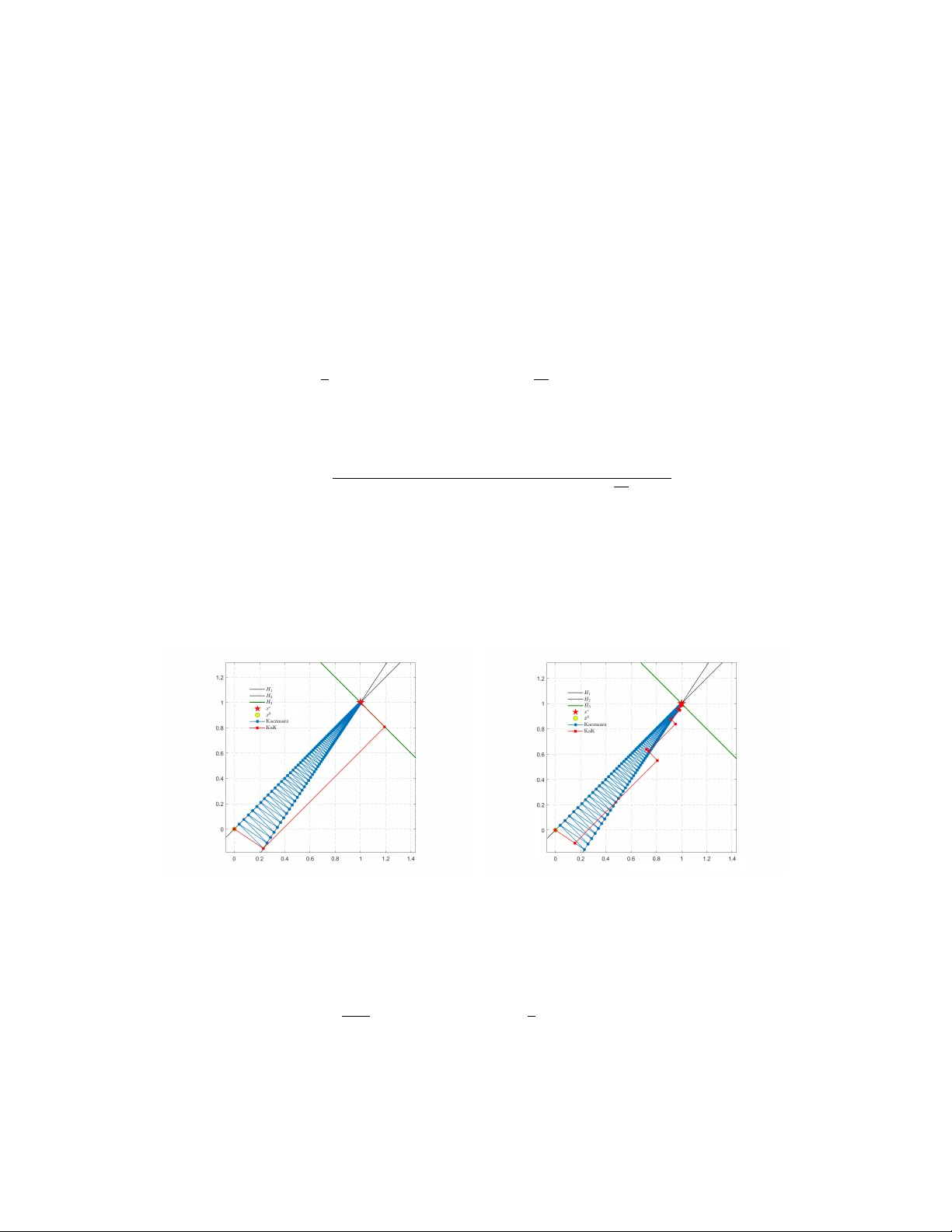
Rob ust Kaczmarz methods f or nearly singular linear systems * Y unying K e † ,1 and Hao Luo ‡ ,1,2 1 National Center for Applied Mathematics in Chongqing, Chongqing Normal University , Chongqing, 401331, China 2 Chongqing Research Institute of Big Data, Peking University , Chongqing, 401121, China February 26, 2026 Abstract The Kaczmarz method is an efficient iterati v e algorithm for large-scale linear systems. Ho we v er , its linear con ver gence rate suffers from ill-conditioned problems and is highly sensitiv e to the smallest nonzero singular value. In this work, we aim to extend the classical Kaczmarz to nearly singular linear systems that are ro w rank-deficient. W e introduce a new concept of nearly singular property by treating the row space as an un- stable subspace in the Grassman manifold. W e then define a related important space called the approximate kernel, based on which a robust kernel-augmented Kaczmarz (KaK) is introduced via the subspace correction framew ork and analyzed by the well-known Xu–Zikatanov identity . T o get an implementable version, we further introduce the approximate dual kernel and transform KaK into an equi v alent kernel-augmented coordi- nate descent. Furthermore, we dev elop an accelerated v ariant and establish the improved rate of con ver gence matching the optimal complexity of first-order methods. Compared with existing methods, ours achieve uni- form conv ergence rates for nearly singular linear systems, and the robustness has been confirmed by some numerical tests. 1 Introduction The Kaczmarz method [ 14 ] is a widely used iterative solver for large linear systems. As a row-action approach, it exactly satisfies one equation per iteration while maintaining very low computational cost per step. This method is highly ef ficient and easy to implement, aligning well with the spirit of the algebraic reconstruction technique [ 12 ]. Consider a consistent linear system: Ax = b, (1) where b ∈ R m belongs to range ( A ) , the range of A ∈ R m × n . Starting from an arbitrary initial vector x 0 ∈ R n , the classical Kaczmarz method [ 14 ] reads as follows x k +1 = x k + b i − A ( i ) x k ∥ A ( i ) ∥ 2 A ⊤ ( i ) , i = k mo d m, (2) where A ( i ) denotes the i -th ro w of A , and b i the i -th component of b . Geometrically , at the k -th iteration, the update x k +1 is the orthogonal projection of x k onto the hyperplane H i = { x ∈ R n : A ( i ) x = b i } , where i = k mo d m . * This work was supported by the National Natural Science Foundation of China (Grant No. 12401402), the Science and T echnology Research Program of Chongqing Municipal Education Commission (Grant Nos. KJZD-K202300505), the Natural Science Foundation of Chongqing (Grant No. CSTB2024NSCQ-MSX0329) and the Foundation of Chongqing Normal Univ ersity (Grant No. 22xwB020). † Email: 2023110510025@stu.cqnu.edu.cn ‡ Email: luohao@cqnu.edu.cn; luohao@cqbdri.pku.edu.cn 1 The randomized strategy serves as one effecti ve approach to accelerate the con v ergence of the Kaczmarz method ( 2 ). Strohmer and V ershynin [ 33 ] proposed the randomized Kaczmarz (RK) x k +1 = x k + b i k − A ( i k ) x k ∥ A ( i k ) ∥ 2 A ⊤ ( i k ) , (3) which selects randomly a row index i k ∈ { 1 , · · · , m } and achiev es an e xponential rate with the contraction factor 1 − 1 /κ 2 ( A ) (see also [ 18 ]), where κ ( A ) := ∥ A ∥ F /σ + min ( A ) and σ + min ( A ) are respectively the scaled condition number [ 5 ] and the smallest nonzero singular value of A . After that, RK has found its applications in CT image reconstruction [ 3 ] and inspired subsequently various extensions, including greedy RK methods [ 1 , 7 , 34 , 35 ], randomized sparse Kaczmarz methods [ 4 , 29 , 48 ], and randomized block Kaczmarz methods [ 8 , 24 , 25 , 38 , 39 , 46 ]. On the other hand, it is well-kno wn that the Kaczmarz method ( 2 ) is equiv alent to applying the coordinate descent (CD) method to the dual problem min y ∈ R m g ( y ) = 1 2 ∥ A ⊤ y ∥ 2 + b ⊤ y . (4) Indeed, for this unconstrained optimization problem, the CD iteration is giv en by y k +1 = y k − sU i U ⊤ i ∇ g ( y k ) , i = k mo d m, (5) where s > 0 denotes the step size, and U i the i -th column of the identity matrix of order m . If s = ∥ A ( i ) ∥ − 2 , then multiplying both sides of ( 5 ) by − A ⊤ recov ers the classical Kaczmarz iteration ( 2 ). Nesterov [ 26 ] proposed a randomized version of ( 5 ) with the rate O (1 /k ) for general conv e x objectiv es. The accelerated coordinate descent method (ACDM) was further dev eloped in [ 26 ] to achie ve a faster rate O (1 /k 2 ) . Applying A CDM to ( 4 ) yields the accelerated randomized Kaczmarz (ARK) [ 17 , 19 ], which the improved contraction factor 1 − m − 1 / 2 /κ ( A ) . For more related works, we refer to [ 6 , 18 , 20 , 36 , 37 , 47 ] and the references therein. Also, as pointed out in [ 10 ], the Kaczmarz method ( 2 ) is a special instance of the Schwarz iterativ e methods [ 9 ], which are also kno wn as the subspace correction methods [ 40 , 41 , 42 ]. Under such a framework, Oswald and Zhou [ 28 ] proved that the cyclic Kaczmarz method con ver ges linearly with a factor of 1 − c/κ 2 ( D − 1 / 2 A ) , where c is a mild logarithmic dependence on m . 1.1 Motivation Although Kaczmarz methods are effecti v e for large-scale noisy or inconsistent systems [ 49 ] and there are also parallel and sparse variants [ 23 , 30 , 45 , 44 ], the rate degenerates for ill-conditioned problems. Such ill-condition systems arise in practical applications like CT reconstruction [ 2 ] and finite element discretizations for H ( grad ) , H ( div ) , and H ( curl ) systems [ 13 ] and stable discretizations of the nearly incompressible elasticity problems [ 43 ]. The theoretical rates depend on the scaled condition number κ ( A ) which can be huge and slow down the con v ergence, especially for nearly singular systems having small nonzero singular values; see also [ 31 ]. Instead of ( 1 ), throughout, let us consider the following linear system A ( ϵ ) x = b, (6) where A ( ϵ ) ∈ R m × n depends on a small parameter ϵ > 0 , and b ∈ range ( A ( ϵ )) ensures the consistency . W e are interested in the limit case ϵ → 0+ , which makes A ( ϵ ) ill-conditioned as σ + min ( A ( ϵ )) → 0 . Look at a simple example A ( ϵ ) =  1 − 1 1 + ϵ − 1 + ϵ  . (7) The two rows are almost identical and λ + min ( A ⊤ ( ϵ ) A ( ϵ )) = 2 + ϵ 2 − √ ϵ 4 + 4 = O ( ϵ 2 ) . As shown in T able 1 , for this instance, decreasing ϵ increases κ ( A ( ϵ )) dramatically , and the Kaczmarz method ( 2 ) becomes inefficient 2 as the two hyperplanes with respect to the ro ws of A ( ϵ ) approach to each other . The heavy zigzag behavior of Kaczmarz can be observed from Fig. 1 . This leads to our main motiv ation: How to pr eserve the efficiency of Kaczmarz methods for nearly singular linear systems? ϵ 1 / 5 1 / 5 2 1 / 5 3 1 / 5 4 κ ( A ( ϵ )) 10 50 250 1 . 25 × 10 3 Kaczmarz 4 . 1 × 10 2 1 . 0 × 10 4 2 . 5 × 10 5 6 . 3 × 10 6 KaK 16 16 16 16 T able 1: The condition number κ ( A ( ϵ )) and iterations of Kaczmarz ( 2 ) and kernel-augmented Kaczmarz ( KaK ) under the stopping criterion: ∥ A ( ϵ ) x − b ∥ / ∥ b ∥ < 10 − 7 . 1.2 Main contributions So far , robust Kaczmarz methods for general non-square nearly singular systems hav e not been considered before in the literature. In this work, we extend the classical Kaczmarz ( 2 ) to the nearly singular problem ( 6 ) and establish the uniformly rate of conv er gence for small ϵ > 0 . More precisely , our main contributions are summarized as below . • W e introduce the concept of near singularity for matrices with unstable ro w spaces and provide detailed characterizations via the canonical angles in the Grassman manifold. As a generalization of the standard kernel space, we also define a related important set called the appr oximate kernel , which is crucial for dev eloping our robust Kaczmarz methods. • Based on the subspace correction presentation [ 10 , 28 ] of Kaczmarz, we propose an variant called the kernel-augmented Kaczmarz (KaK), which adopts a stable ro w space decomposition by using the approx- imate kernel and possesses a robust linear rate O ((1 − ρ ) k ) , where ρ ∈ (0 , 1) is uniformly independent on the small parameter ϵ . W e refer to T able 1 for numerical evidence on the simple example ( 7 ). • Using the relation between Kaczmarz and CD, we deri ve an equi v alent and implementable version of KaK called the kernel-augmented CD (KaCD). Also, we combine KaCD with a predictor -corrector scheme [ 22 , Eq.(83)] yielding the kernel-augmented accelerated coordinate descent (KaACD). The uniform faster rate O (min  1 /k 2 , (1 − √ ρ ) k  ) shall be prov ed theoretically and verified numerically . T o the best of our knowledge, KaK is the first rob ust Kaczmarz with a stable rate of con ver gence for nearly singular systems, and KaA CD is the first accelerated coordinate descent with robust linear rate, compared with existing acceleration works [ 17 , 19 ]. 1.3 Outline The remainder of the paper is org anized as follows. In Section 2 we prepare some preliminaries including basic notations, the Grassman manifold and the subspace correction frame work. In Section 3 we introduce the near singularity and the approximate kernel. Then in Section 4 we give our robust Kaczmarz method and establish the proof of con ver gence rate. The equi v alent KaCD and its acceleration are presented in Section 5 . Numerical experiments are provided in Section 6 and finally , Section 7 gives some concluding remarks. 2 Preliminaries In this section, we prepare some preliminaries including basic notations, the Grassman manifold and the sub- space correction framew ork. 3 2.1 Notation Let V be a finite dimensional Hilbert space with the inner product ( · , · ) and the induced norm ∥·∥ = p ( · , · ) . Denote by L ( V ) the set of all linear mappings from V to V . The identity mapping I : V → V is I v = v for all v ∈ V . If W ⊂ V is a subspace, then define the inclusion operator ι W → V : W → V by the restriction of the identity operator on W , i.e., ι W → V = I W . Giv en any A ∈ L ( V ) , the operator norm is ∥ A ∥ V → V := sup ∥ v ∥ =1 ∥ Av ∥ , and the adjoint operator A ′ : V → V is defined by ( A ′ u, v ) = ( u, Av ) ∀ u, v ∈ V . (8) When A is symmetric and positive definite (SPD), i.e., A = A ′ and ⟨ Av , v ⟩ > 0 for all v ∈ V \{ 0 } , we also define the A -inner product ( u, v ) A := ( Au, v ) ∀ u, v ∈ V , (9) and the induced A -norm ∥·∥ A := p ( · , · ) A . For any B ∈ L ( V ) , its A -norm is defined by ∥ B ∥ A := sup ∥ v ∥ A =1 ∥ B v ∥ A , and we denote by B t : V → V the adjoint operator of B with respect to (w .r .t.) the A -inner product:  B t u, v  A = ( u, B v ) A ∀ u, v ∈ V . (10) Clearly , for any B ∈ L ( V ) , we have ( B A ) t = B ′ A . Particularly , if B = B ′ is symmetric, then ( B A ) t = B A , which means B A is symmetric w .r .t the A -inner product. As usual, let ∥·∥ be the standard 2-norm of vectors/matrices and ⟨· , ·⟩ the Euclidean inner product between vectors. For a linear subspace S ⊂ R n , dim( S ) refers to its dimension. For any C ∈ R m × n , denote by C ⊤ /C + the transpose/ Moore-Penrose pseudoin v erse of C and let rank C, ker ( C ) and range ( C ) be the rank, the kernel space and the range (or column space) of C , respectively . The range of C ⊤ is called the row space of C and usually denoted as ro w ( C ). A fundamental fact is that row ( C ) = row ( C ⊤ C ) for all C ∈ R m × n , which implies dim( row ( C )) = rank ( C C ⊤ ) . For a symmetric matrix C ∈ R n × n , let λ min ( C ) and λ max ( C ) be the smallest and largest eigen values of C . If C is symmetric positiv e semidefinite, then denote by λ + min ( C ) the smallest nonzero eigen v alue of C , namely , λ + min ( C ) := min v ∈ range ( C ) \{ 0 } ⟨ C v , v ⟩ / ∥ v ∥ 2 . (11) 2.2 The Grassman manif old Let n, p ∈ N + be such that p ≤ n . The Grassman manifold Grass ( p, n ) consists of all p -dimensional subspaces of R n . For any nonzero vectors u, w ∈ R n \{ 0 } , the angle between u and w is ∠ ( u, w ) := arccos ⟨ u, w ⟩ ∥ u ∥∥ w ∥ ∈ [0 , π ] . As an generalization, for any u ∈ R n \{ 0 } and W ∈ Grass ( p, n ) , the angle between u and W is defined by ∠ ( u, W ) := min w ∈ W \{ 0 } arccos |⟨ u, w ⟩| ∥ u ∥∥ w ∥ ∈ [0 , π / 2] . (12) Let P W : R n → W be the orthogonal projection, then ∠ ( u, W ) = arccos ∥ P W u ∥ / ∥ u ∥ . 4 Definition 2.1 (Canonical angles) . F or any U, W ∈ Grass ( p, n ) , assume the columns of U ∈ R n × p and W ∈ R n × p form orthonormal bases of U and W . Let 0 ≤ σ 1 ≤ · · · ≤ σ p be the singular values of U ⊤ W . F or 1 ≤ i ≤ p , define θ i := arccos σ i ∈ [0 , π / 2] . W e call 0 ≤ θ p ≤ · · · ≤ θ 1 ≤ π / 2 the canonical angles between U and W . The largest canonical angle θ 1 satisfies cos θ 1 = min u ∈ U \{ 0 } max w ∈ W \{ 0 } |⟨ u, w ⟩| ∥ u ∥ ∥ w ∥ . Remark 2.1. F or given U, W ∈ Grass ( p, n ) , the canonical angles { θ i } p i =1 is independent on the choices of the orthonormal bases of U and W . In particular , we can take U = [ u 1 , · · · , u p ] and W = [ w 1 , · · · , w p ] such that ⟨ u i , u j ⟩ = ⟨ w i , w j ⟩ = δ ij and ⟨ u i , w j ⟩ = δ ij cos θ i for all 1 ≤ i, j ≤ p . Definition 2.2 (Gap metric on Grass ( p, n ) ) . F or any U, W ∈ Grass ( p, n ) , define the gap metric by that ∆( U, W ) := ∥ P U − P W ∥ , wher e P U : R n → U and P W : R n → W ar e orthogonal pr ojection operator s. It is well-kno wn that the Grassman manifold Grass ( p, n ) equipped with the gap metric ∆( · , · ) yields a complete metric space. For any U, W ∈ Grass ( p, n ) , according to [ 32 , Theorem 4.5 and Corollary 4.6], we hav e ∆( U, W ) = sin θ 1 , (13) where θ 1 ∈ [0 , π / 2] denotes the largest canonical angle between U and W . In particular , we hav e ∠ ( u, row ( v ⊤ )) = ∠ ( ro w ( u ⊤ ) , row ( v ⊤ )) for any u, v ∈ R n \{ 0 } . Lemma 2.1. Let A : [0 , δ ] → R m × n be a matrix-valued function that is continuous in component-wise. If ro w ( A ( ϵ )) ∈ Grass ( r, n ) for all ϵ ∈ [0 , δ ] , then lim ϵ → 0+ ∆( ro w ( A ( ϵ )) , row ( A (0))) = 0 . Pr oof. The orthogonal projection operator P A ( ϵ ) : R n → row ( A ( ϵ )) is giv en by P A ( ϵ ) = A ⊤ ( ϵ )  A ( ϵ ) A ⊤ ( ϵ )  † A ( ϵ ) , where ( · ) † denotes the Moore–Penrose pseudoin v erse. Since A ( ϵ ) is continuous in component-wise and ro w ( A ( ϵ )) ∈ Grass ( r, n ) for all ϵ ∈ [0 , δ ] , we claim that A ( ϵ ) A ⊤ ( ϵ ) is also continuous and rank A ( ϵ ) A ⊤ ( ϵ ) = dim row ( A ( ϵ )) = r for all ϵ ∈ [0 , δ ] . Thanks to [ 32 , Theorem 3.9],  A ( ϵ ) A ⊤ ( ϵ )  † is continuous and so is P A ( ϵ ) . In particular, by Definition 2.2 , we hav e lim ϵ → 0+ ∆( ro w ( A ( ϵ )) , row ( A (0))) = lim ϵ → 0+ ∥ P A ( ϵ ) − P A (0) ∥ = 0 . This completes the proof of this lemma. ■ Lemma 2.2. Let u, v ∈ R n \{ 0 } and W ∈ Grass ( p, n ) be such that ∠ ( u, W ) ≤ β and ∠ ( v , W ) ≥ θ , with 0 ≤ β ≤ θ ≤ π / 2 . Then cos ∠ ( u, v ) ≤ cos( θ − β ) . Pr oof. W ith out loss of generality , assume u and v are unit vectors. Then cos ∠ ( u, W ) = ∥ P W u ∥ and cos ∠ ( v , W ) = ∥ P W v ∥ , and we hav e the orthogonal decomposition: u = P W u + u 0 and v = P W v + v 0 , where both u 0 = u − P W u and v 0 = v − P W v are orthogonal to W . Observing sin ∠ ( u, W ) = ∥ u 0 ∥ and sin ∠ ( v , W ) = ∥ v 0 ∥ , a direct calculation giv es cos ∠ ( u, v ) = ⟨ u, v ⟩ = ⟨ P W u, P W v ⟩ + ⟨ u 0 , v 0 ⟩ = ∥ P W u ∥ ∥ P W v ∥ cos ∠ ( P W u, P W v ) + ∥ u 0 ∥ ∥ v 0 ∥ cos ∠ ( u 0 , v 0 ) = cos ∠ ( u, W ) cos ∠ ( v , W ) cos ∠ ( P W u, P W v ) + sin ∠ ( u, W ) sin ∠ ( v , W ) cos ∠ ( u 0 , v 0 ) ≤ cos ∠ ( u, W ) cos ∠ ( v , W ) + sin ∠ ( u, W ) sin ∠ ( v , W ) = cos( ∠ ( u, W ) − ∠ ( v , W )) = cos( ∠ ( v , W ) − ∠ ( u, W )) . Since − ∠ ( u, W ) ≥ − β and ∠ ( v , W ) ≥ θ , we obtain ∠ ( v , W ) − ∠ ( u, W ) ≥ θ − β ≥ 0 . It follows immediately that cos ∠ ( u, v ) ≤ cos( θ − β ) . This completes the proof. ■ 5 2.3 Successive subspace correction Let V be a finite dimensional Hilbert space with the inner product ( · , · ) and the induced norm ∥·∥ = p ( · , · ) . Giv en an SPD linear operator A : V → V and f ∈ V , we aim to seek u ∈ V such that Au = f . (14) Let us restate briefly the basic framework of the successive subspace corr ection (SSC) for solving ( 14 ); see [ 40 , 41 , 42 ] for a comprehensiv e presentation. Such a frame work is crucial for us to analyze the Kaczmarz iteration and dev elop robust variants for solving nearly singular system. 2.3.1 Algorithm presentation Consider a finite sequence of finite dimensional auxiliary spaces { V j } J j =1 . Each V j is not necessarily a subspace of V but is related to V via a linear operator R j : V j → V that satisfies the following decomposition assumption. Assumption 1. It holds that V = P J j =1 R j V j . Thanks to Assumption 1 , for any v ∈ V , we hav e v = P J j =1 R j v j with v j ∈ V j , 1 ≤ j ≤ J . Here we do not require such a decomposition is a direct sum, i.e., the representation of v has not to be unique. For each auxiliary space, we also propose the following assumption. Assumption 2. F or 1 ≤ j ≤ J , V j is a Hilbert space with an inner pr oduct a j ( · , · ) . Let R ∗ j : V → V j be the adjoint operator of R j , namely , a j  R ∗ j v , v j  = ( v , R j v j ) ∀ v j ∈ V j , v ∈ V . Define the linear operator T j : V → V j by that a j ( T j v , v j ) = ( v , R j v j ) A ∀ v j ∈ V j , v ∈ V . Clearly , T j is the adjoint operator of R j w .r .t. the A -inner product and T j = R ∗ j A . Note that R j R ∗ j : V → V is symmetric and thus R j T j = R j R ∗ j A is symmetric w .r .t. the A -inner product. The method of SSC with relaxation reads as follows (cf.[ 40 , Algorithm 3.5]). Gi ven u k ∈ V , set v k, 1 = u k and update u k +1 = v k,J +1 by v k,j +1 = v k,j + ω R j R ∗ j ( f − Av k,j ) for j = 1 , · · · , J, (15) where ω > 0 denotes the relaxation parameter . It can be reformulated as a multiplicativ e Schwarz iteration u k +1 = u k + B ssc ( ω )( f − Au k ) , (16) with the iterator B ssc ( ω ) : V → V satisfies I − B ssc ( ω ) A = ( I − ω R J T J ) · · · ( I − ω R 1 T 1 ) . 2.3.2 Symmetrization Note that B ssc ( ω ) is possibly not symmetric and the symmetrized variant of ( 16 ) is useful for both theoretical analysis and practical performance. Specifically , based on ( 16 ), consider ( u k +1 / 2 = u k + B ssc ( ω )( f − Au k ) , u k +1 = u k +1 / 2 + B ′ ssc ( ω )( f − Au k +1 / 2 ) , where B ′ ssc ( ω ) : V → V denotes the adjoint operator of B ssc ( ω ) ; see ( 8 ). This yields the symmetrized SSC [ 40 , Algorithm 3.4]. Gi ven u k ∈ V , update u k +1 ∈ V by the following two steps: 6 • Step 1 Set v k, 1 = u k and update u k +1 / 2 = v k,J +1 by v k,j +1 = v k,j + ω R j R ∗ j ( f − Av k,j ) for j = 1 , · · · , J. • Step 2 Set v k,J +1 = u k +1 / 2 and update u k +1 = v k, 1 by that v k,j = v k,j +1 + ω R j R ∗ j ( f − Av k,j +1 ) for j = J, · · · , 1 . Actually , this is also equiv alent to a multiplicative Schwarz iteration u k +1 = u k + ¯ B ssc ( ω )( f − Au k ) , (17) where ¯ B ssc ( ω ) = B ′ ssc ( ω ) + B ssc ( ω ) − B ′ ssc ( ω ) AB ssc ( ω ) is called the symmetrization of B ssc ( ω ) . Similarly as before, a direct computation giv es I − ¯ B ssc ( ω ) A = ( I − B ′ ssc ( ω ) A )( I − B ssc ( ω ) A ) = ( I − B ssc ( ω ) A ) t ( I − B ssc ( ω ) A ) , (18) which is symmetric w .r .t. the A -inner product. 2.3.3 Con vergence theory Based on Assumption 1 , we introduce an auxiliary space of product type V := V 1 × V 2 × · · · × V J and the corresponding inner product ( u , v ) V := P J j =1 a j ( u j , v j ) for all u , v ∈ V with u j = u j and v j = v j . The induced norm is ∥·∥ V := p ( · , · ) V . Define the linear operator R : V → V by that R u = J X j =1 R j u j = J X j =1 R j u j . W e claim that R : V → V is onto, i.e., R is surjective. Denote by R ⋆ : V → V the adjoint operator of R : ( R ⋆ u, v ) V = ( u, R v ) . W e also define the adjoint operator of R w .r .t. the A -inner product:  R T u, v  V = ( u, R v ) A . (19) It is clear that R T = ( A R ) ⋆ = R ⋆ A . Let A = R ⋆ A R be the expanded operator . If we write each v ∈ V as a “column vector", then in a consistent block form, we hav e R = ( R 1 , · · · , R J ) and A =       T 1 R 1 T 1 R 2 · · · T 1 R J T 2 R 1 T 2 R 2 · · · T 2 R J . . . . . . . . . . . . T J R 1 T J R 2 · · · T J R J       , R ⋆ =       R ∗ 1 R ∗ 2 . . . R ∗ J       , v =       v 1 v 2 . . . v J       . Now consider the block splitting A = D + L + U , where D = diag ( A ) denotes the block diagonal part and U = triu ( A ) is the strict upper block triangular part. It is not hard to verify that L ′ = U and D ′ = D . Under the following assumption, which is equiv alent to that 2 I − ω D is SPD, we can establish the conv er- gence results of ( 16 ) and ( 17 ). It is kno wn as the famous Xu–Zikatanov identity [ 42 ] and provides a powerful tool for the analysis of the Kaczmarz iteration and its variants. Assumption 3. 2 I − ω D is SPD. Or equivalently , ω ∈ (0 , 2 / ∥ D ∥ V → V ) . 7 Theorem 2.1 ([ 42 ]) . Under Assumptions 1 , 2 and 3 , both ( 16 ) and ( 17 ) ar e conver gent and   I − ¯ B ssc ( ω ) A   A = ∥ I − B ssc ( ω ) A ∥ 2 A = 1 − 1 c 0 ( ω ) , (XZ-Identity) wher e the finite positive constant c 0 ( ω ) is defined by c 0 ( ω ) := 1 ω sup ∥ v ∥ A =1 inf R v = v  (2 I − ω D ) − 1 ( I + ω U ) v , ( I + ω U ) v  V (20) As an important byproduct, we hav e the follo wing corollary . Corollary 2.1. Under Assumptions 1 , 2 and 3 , for the symmetrized iterator ¯ B ssc ( ω ) , we have 1 c 0  ¯ B − 1 ssc ( ω ) v, v  ≤ ⟨ Av , v ⟩ ≤  ¯ B − 1 ssc ( ω ) v, v  ∀ v ∈ V , (21) wher e c 0 ≥ c 0 ( ω ) is arbitrary , with c 0 ( ω ) > 0 being given by ( 20 ) . Pr oof. W e refer to [ 40 , Lemma 2.1] and omit the details. ■ 3 Nearly Singularity Property In [ 16 ], Lee et al. considered a special nearly singular case with A ( ϵ ) = ϵI + A 0 , where A 0 is symmetric positiv e semidefinite. It is clear that A ( ϵ ) is SPD for all ϵ > 0 but λ min ( A ( ϵ )) → 0 as ϵ → 0 . In this section, we aim to extend such a nearly singular property to a more general non-square case. 3.1 Definition As we all know , the Kaczmarz iteration is actually a row action method [ 14 ] and can also be recast into the SSC framework [ 28 , 42 ] with proper subspace decomposition on the row space of A ( ϵ ) ; see later in Section 4 . Motiv ated by this, instead of the degenerac y of the smallest eigenv alue or singular value, we now focus on the asymptotic beha vior of row ( A ( ϵ )) as ϵ approaches to 0. More precisely , assume that A ( ϵ ) admits the two-block structure as specified below in Assumption 4 . Assumption 4. Let ¯ ϵ > 0 . The matrix-valued function A : [0 , ¯ ϵ ] → R m × n is continuous in component-wise and admits the two-block structure A ( ϵ ) = " A 0 ( ϵ ) A 1 ( ϵ ) # ∀ 0 ≤ ϵ ≤ ¯ ϵ, (22) wher e A 0 ( ϵ ) ∈ R m 0 × n and A 1 ( ϵ ) ∈ R m 1 × n with m 0 + m 1 = m . Moreover , the diagonal part D ϵ := diag  A ( ϵ ) A ⊤ ( ϵ )  : [0 , ¯ ϵ ] → R m × m is non-de gener ate η 0 I ⪯ D ϵ ⪯ η 1 I ∀ 0 ≤ ϵ ≤ ¯ ϵ, (23) wher e 0 < η 0 ≤ η 1 < ∞ ar e independent on ϵ . From the SSC perspecti ve, the stability of the row space plays a key role. Inspired by this, we introduce the following definition of nearly singular pr operty that leads to the unstable subspace decomposition. Definition 3.1 (Nearly singular property) . Let A : [0 , ¯ ϵ ] → R m × n be a matrix-valued function satisfying Assumption 4 . W e say that A ( ϵ ) is nearly singular at ϵ = 0 (or simply nearly singular) if it satisfies: (i) dim ro w ( A 0 ( ϵ )) < dim row ( A ( ϵ )) for all 0 < ϵ ≤ ¯ ϵ ; 8 (ii) ther e exists r 0 ∈ N + such that dim ro w ( A 0 ( ϵ )) = r 0 for all 0 ≤ ϵ ≤ ¯ ϵ ; (iii) ther e is Π ∈ R m 1 × m 0 such that A 1 (0) = Π A 0 (0) . In other words, we have row ( A (0)) ⊂ ro w ( A 0 (0)) . Let us discuss briefly the above definition. The first term says that ro w ( A 0 ( ϵ )) is indeed a proper subspace of ro w ( A ( ϵ )) ; the second implies that the dimension of row ( A 0 ( ϵ )) leaves in v ariant for all ϵ ∈ [0 , ¯ ϵ ] and is continuous at ϵ = 0 . Notably , as ϵ → 0+ , row ( A 0 ( ϵ )) con ver ges to row ( A 0 (0)) under the gap metric. Lemma 3.1. Let A : [0 , ¯ ϵ ] → R m × n satisfy Assumption 4 . If A ( ϵ ) is nearly singular , then row ( A 0 ( ϵ )) ∈ Grass ( r 0 , n ) for all ϵ ∈ [0 , ¯ ϵ ] and lim ϵ → 0+ ∆( ro w ( A 0 ( ϵ )) , row ( A 0 (0))) = 0 , wher e ∆( · , · ) denotes the gap metric (cf.Definition 2.2 ). Pr oof. Applying Lemma 2.1 to A 0 : [0 , ¯ ϵ ] → R m × n concludes the proof. ■ Howe ver , for the whole row space row ( A ( ϵ )) , the dimension r eduction occurs at ϵ = 0 due to the inclusion relation in the third term in Definition 3.1 . If we consider a decomposition of row ( A ( ϵ )) by the row vectors, then it is unstable when ϵ → 0+ . For instance, let A ( ϵ ) be given by ( 7 ), which has row ( A ( ϵ )) = R 2 for all ϵ > 0 . W ith A 0 ( ϵ ) = [1 , − 1] and A 1 ( ϵ ) = [1 + ϵ, − 1 + ϵ ] , it is clear that dim row ( A 0 ( ϵ )) = 1 for all ϵ ≥ 0 . Hence, by Definition 3.1 , A ( ϵ ) is nearly singular . 3.2 A pproximate ker nel W e then introduce the appr oximate kernel of a nearly singular matrix A ( ϵ ) , which is crucial for us to de velop a robust iterative method from the SSC framework. Definition 3.2 (Approximate kernel) . Let A : [0 , ¯ ϵ ] → R m × n be a matrix-valued function satisfying Assump- tion 4 . The appr oximate kernel of A ( ϵ ) is defined by k er ϵ ( A ( ϵ )) := k er ( A 0 ( ϵ )) ∩ ro w ( A ( ϵ )) = n A ⊤ ( ϵ ) y : A 0 ( ϵ ) A ⊤ ( ϵ ) y = 0 , y ∈ R m o . (24) The appr oximate dual kernel of A ( ϵ ) is given by d k er ϵ ( A ( ϵ )) := ker ( A 0 ( ϵ ) A ⊤ ( ϵ )) =  y ∈ R m : A 0 ( ϵ ) A ⊤ ( ϵ ) y = 0  . (25) W e claim that the approximate kernel ker ϵ ( A ( ϵ )) is actually the orthogonal complement of ro w ( A 0 ( ϵ )) in ro w ( A ( ϵ )) ; see the proof of Lemma 3.3 . In addition, ker ϵ ( A ( ϵ )) is the image of the approximate dual kernel d k er ϵ ( A ( ϵ )) under the mapping A ⊤ ( ϵ ) : R m → R n . It follows that dim ker ϵ ( A ( ϵ )) ≤ dim d k er ϵ ( A ( ϵ )) . When A ( ϵ ) has full row rank, the equality case dim k er ϵ ( A ( ϵ )) = dim d k er ϵ ( A ( ϵ )) holds. Note that our Definition 3.1 does not inv olv e explicitly the de generate behavior of the singular values of A ( ϵ ) . In the follo wing, we establish an upper bound of λ + min ( A ⊤ ( ϵ ) A ( ϵ )) , which goes to zero as ϵ → 0+ . Lemma 3.2. Let A : [0 , ¯ ϵ ] → R m × n satisfy Assumption 4 and a ⊤ i ( ϵ ) the i -th r ow of A 1 ( ϵ ) for 1 ≤ i ≤ m 1 . Let θ 1 ( ϵ ) ∈ [0 , π / 2] denote the lar g est canonical angle between row ( A 0 ( ϵ )) and row ( A 0 (0)) , and define β ( ϵ ) := max 1 ≤ i ≤ m 1 β i ( ϵ ) with β i ( ϵ ) = ∠ ( a i ( ϵ ) , row ( A 1 (0))) ∈ [0 , π / 2] . If A ( ϵ ) is nearly singular , then θ 1 ( ϵ ) + β ( ϵ ) → 0 as ϵ → 0+ , (26) which implies there exists some ϵ 0 ∈ (0 , ¯ ϵ ] such that 0 ≤ θ 1 ( ϵ ) + β ( ϵ ) ≤ π / 2 ∀ ϵ ∈ [0 , ϵ 0 ] . (27) In addition, we have the estimate λ + min ( A ⊤ ( ϵ ) A ( ϵ )) ≤ m 1 η 1 sin 2 ( θ 1 ( ϵ ) + β ( ϵ )) ∀ ϵ ∈ [0 , ϵ 0 ] . (28) 9 Pr oof. Let us firstly verify the statement ( 26 ). From ( 13 ), we claim that θ 1 ( ϵ ) = arcsin ∆( row ( A 0 ( ϵ )) , row ( A 0 (0))) is continuous and it follo ws from Lemma 3.1 that θ 1 ( ϵ ) → 0 as ϵ → 0+ . For 1 ≤ i ≤ m 1 , a i : [0 , ¯ ϵ ] → R n is continuous and ro w ( a ⊤ i ( ϵ )) ∈ Grass (1 , n ) for all 0 ≤ ϵ ≤ ¯ ϵ . Then we find that β i ( ϵ ) = ∠ ( a i ( ϵ ) , row ( A 1 (0))) ≤ ∠ ( a i ( ϵ ) , row ( a ⊤ i (0))) = ∠ ( row ( a i ( ϵ )) , row ( a ⊤ i (0))) = arcsin ∆( row ( a ⊤ i ( ϵ )) , row ( a ⊤ i (0))) . Thus, by Lemma 2.1 , we have β i ( ϵ ) → 0 as ϵ → 0+ , which yields that β ( ϵ ) → 0 as ϵ → 0+ and concludes ( 26 ). It is clear that β ( ϵ ) is continuous and there exists some ϵ 0 ∈ (0 , ¯ ϵ ] such that θ 1 ( ϵ ) + β ( ϵ ) ∈ [0 , π / 2] for all ϵ ∈ [0 , ϵ 0 ] . This verifies ( 27 ). In what follows, let us prove the estimate ( 28 ). It is evident that (cf.( 11 )) λ + min ( A ⊤ ( ϵ ) A ( ϵ )) = min v ∈ row ( A ( ϵ )) \{ 0 } ∥ A ( ϵ ) v ∥ 2 / ∥ v ∥ 2 . Here, we used the fact range ( A ⊤ ( ϵ ) A ( ϵ )) = range ( A ⊤ ( ϵ )) = row ( A ( ϵ )) . Since A ( ϵ ) is nearly singular , by Definition 3.1 , we must have dim ker ϵ ( A ( ϵ )) = dim row ( A ( ϵ )) − r 0 > 0 for all ϵ ∈ (0 , ¯ ϵ ] . Therefore, for any unit vector v ( ϵ ) ∈ k er ϵ ( A ( ϵ )) , it follows λ + min ( A ⊤ ( ϵ ) A ( ϵ )) ≤ ∥ A ( ϵ ) v ( ϵ ) ∥ 2 = ∥ A 1 ( ϵ ) v ( ϵ ) ∥ 2 = m 1 X i =1 | ⟨ a i ( ϵ ) , v ( ϵ ) ⟩ | 2 ≤ max 1 ≤ i ≤ m 1 cos 2 ∠ ( v ( ϵ ) , a i ( ϵ )) · m 1 X i =1 ∥ a i ( ϵ ) ∥ 2 ≤ m 1 η 1 max 1 ≤ i ≤ m 1 cos 2 ∠ ( v ( ϵ ) , a i ( ϵ )) , (29) where in the last line, we used the assumption ( 23 ), which promises ∥ a i ( ϵ ) ∥ 2 ≤ η 1 for all 1 ≤ i ≤ m 1 . It is sufficient to find an upper bound estimate of cos ∠ ( v ( ϵ ) , a i ( ϵ )) , which is equiv alent to get a lower bound of ∠ ( v ( ϵ ) , a i ( ϵ )) for all 1 ≤ i ≤ m 1 . For that, we aim to find a lower bound of ∠ ( v ( ϵ ) , row ( A 0 (0))) and an upper bound of ∠ ( a i ( ϵ ) , row ( A 0 (0))) . According Definition 3.1 , we hav e ro w ( A 1 (0)) ⊂ row ( A 0 (0)) , which indicates that ∠ ( a i ( ϵ ) , row ( A 0 (0))) ≤ ∠ ( a i ( ϵ ) , row ( A 1 (0))) = β i ( ϵ ) ≤ β ( ϵ ) . (30) Then, consider any unit vector u ∈ ro w ( A 0 (0)) , which admits the unique decomposition u = u 1 + u 2 with u 1 ∈ ro w ( A 0 ( ϵ )) and u 2 ∈ k er ( A 0 ( ϵ )) . It is easy to find that ∥ u 1 ∥ = cos ∠ ( u, row ( A 0 ( ϵ ))) and ∥ u 2 ∥ = sin ∠ ( u, ro w ( A 0 ( ϵ ))) ≤ sin θ 1 ( ϵ ) , since θ 1 ( ϵ ) is the largest canonical angle between row ( A 0 ( ϵ )) and ro w ( A 0 (0)) . Observing v ( ϵ ) is orthogonal to u 1 , we also obtain | ⟨ v ( ϵ ) , u ⟩ | = | ⟨ v ( ϵ ) , u 2 ⟩ | ≤ ∥ v ( ϵ ) ∥ ∥ u 2 ∥ = ∥ u 2 ∥ ≤ sin θ 1 ( ϵ ) for any unit vector u ∈ ro w ( A 0 (0)) . Thus, we conclude that ∠ ( v ( ϵ ) , row ( A 0 (0))) ≥ π / 2 − θ 1 ( ϵ ) . (31) Finally , thanks to ( 27 ), ( 30 ) and ( 31 ), in voking Lemma 2.2 yields cos ∠ ( v ( ϵ ) , a i ( ϵ )) ≤ cos( π / 2 − θ 1 ( ϵ ) − β ( ϵ )) = sin( θ 1 ( ϵ ) + β ( ϵ )) , for all 1 ≤ i ≤ m 1 . This together with ( 29 ) gi ves ( 28 ) and completes the proof. ■ As a comparison, we prove that λ + min ( A ⊤ 0 ( ϵ ) A 0 ( ϵ )) is bounded below by a small perturbation of λ + min ( A ⊤ 0 (0) A 0 (0)) , which is independent of ϵ . This is crucial for proving the robust con v ergence rates of our proposed methods. Lemma 3.3. Let A : [0 , ¯ ϵ ] → R m × n be a matrix-valued function satisfying Assumption 4 . If A ( ϵ ) is nearly singular , then we have the orthogonal dir ect sum row ( A ( ϵ )) = ker ϵ ( A ( ϵ )) ⊕ ro w ( A 0 ( ϵ )) , and there exists ϵ 1 ∈ (0 , ¯ ϵ ] such that σ 0 ( ϵ ) := λ + min ( A ⊤ 0 (0) A 0 (0)) cos 2 θ 1 ( ϵ ) − ∥ A 0 (0) − A 0 ( ϵ ) ∥ 2 > 0 ∀ ϵ ∈ [0 , ϵ 1 ] , (32) 10 wher e θ 1 ( ϵ ) ∈ [0 , π / 2] denotes the larg est canonical angle between ro w ( A 0 ( ϵ )) and ro w ( A 0 (0)) . Mor eover , we have λ + min ( A ⊤ 0 ( ϵ ) A 0 ( ϵ )) ≥ σ 0 ( ϵ ) > 0 for all ϵ ∈ [0 , ϵ 1 ] and lim ϵ → 0+ σ 0 ( ϵ ) = λ + min ( A ⊤ 0 (0) A 0 (0)) . (33) Pr oof. Denote by row ( A 0 ( ϵ )) ⊥ the orthogonal complement of row ( A 0 ( ϵ )) in row ( A ( ϵ )) . Let us first show that ker ϵ ( A ( ϵ )) = ro w ( A 0 ( ϵ )) ⊥ . By the definition ( 24 ), ker ϵ ( A ( ϵ )) = k er ( A 0 ( ϵ )) ∩ row ( A ( ϵ )) . Since row ( A 0 ( ϵ )) ⊂ row ( A ( ϵ )) and row ( A 0 ( ϵ )) is orthogonal to ker ( A 0 ( ϵ )) , we hav e ker ϵ ( A ( ϵ )) ⊂ ro w ( A 0 ( ϵ )) ⊥ . It follo ws that dim ker ϵ ( A ( ϵ )) ≤ dim row ( A 0 ( ϵ )) ⊥ = dim ro w ( A ( ϵ )) − dim row ( A 0 ( ϵ )) = dim ro w ( A ( ϵ )) − r 0 . On the other hand, observe the formula dim ker ϵ ( A ( ϵ )) = dim ro w ( A ( ϵ )) + dim ker ( A 0 ( ϵ )) − dim( row ( A ( ϵ )) + ker ( A 0 ( ϵ ))) ≥ dim ro w ( A ( ϵ )) + n − r 0 − n = dim row ( A ( ϵ )) − r 0 , which yields the relation dim k er ϵ ( A ( ϵ )) = dim row ( A 0 ( ϵ )) ⊥ . Hence, we conclude that ker ϵ ( A ( ϵ )) = ro w ( A 0 ( ϵ )) ⊥ and the orthogonal decomposition ro w ( A ( ϵ )) = k er ϵ ( A ( ϵ )) ⊕ row ( A 0 ( ϵ )) holds. According to ( 13 ) and Lemma 3.1 , we claim that θ 1 ( ϵ ) → 0 as ϵ → 0+ , and by Assumption 4 , ∥ A 0 (0) − A 0 ( ϵ ) ∥ → 0 as ϵ → 0+ . This concludes ( 32 ) and ( 33 ). It remain to verify λ + min ( A ⊤ 0 ( ϵ ) A 0 ( ϵ )) ≥ σ 0 ( ϵ ) . For any v ∈ ro w ( A 0 ( ϵ )) , we have the orthogonal decom- position v = v n + v r , where v n ∈ ker ( A 0 (0)) and v r ∈ row ( A 0 (0)) . Since θ 1 ( ϵ ) ∈ [0 , π / 2] denotes the largest canonical angle between row ( A 0 ( ϵ )) and row ( A 0 (0)) , we also get ∥ v n ∥ = ∥ v ∥ sin ∠ ( v , ro w ( A 0 (0))) ≤ ∥ v ∥ sin θ 1 ( ϵ ) , implying ∥ v r ∥ 2 = ∥ v ∥ 2 − ∥ v n ∥ 2 ≥ (1 − sin 2 θ 1 ( ϵ )) ∥ v ∥ 2 = cos 2 θ 1 ( ϵ ) ∥ v ∥ 2 . Thus, it follo ws that ∥ A 0 ( ϵ ) v ∥ 2 ≥ 1 2 ∥ A 0 (0) v ∥ 2 − ∥ ( A 0 (0) − A 0 ( ϵ )) v ∥ 2 = 1 2 ∥ A 0 (0) v r ∥ 2 − ∥ ( A 0 (0) − A 0 ( ϵ )) v ∥ 2 ≥ λ + min ( A ⊤ 0 (0) A 0 (0)) ∥ v r ∥ 2 − ∥ A 0 (0) − A 0 ( ϵ ) ∥ 2 ∥ v ∥ 2 ≥ σ 0 ( ϵ ) ∥ v ∥ 2 . This leads to λ + min ( A ⊤ 0 ( ϵ ) A 0 ( ϵ )) ≥ σ 0 ( ϵ ) and completes the proof. ■ T o the end of this section, we provide three examples for further illustrations. Example 1. Let A ( ϵ ) be given by ( 7 ) , which is nearly singular with A 0 ( ϵ ) = [1 , − 1] and A 1 ( ϵ ) = [1 + ϵ, − 1 + ϵ ] . A dir ect calculation gives A 0 ( ϵ ) A ⊤ ( ϵ ) = [2 , 2] , which yields d k er ϵ ( A ( ϵ )) = span { [1 , − 1] ⊤ } and ker ϵ ( A ( ϵ )) = A ⊤ ( ϵ ) d k er ϵ ( A ( ϵ )) = span { [1 , 1] ⊤ } . Besides, we have λ + min ( A ⊤ 0 ( ϵ ) A 0 ( ϵ )) = 2 and λ + min ( A ⊤ ( ϵ ) A ( ϵ )) = 2 − √ ϵ 4 + 4 + ϵ 2 = O ( ϵ 2 ) . Example 2. Consider a tridiagonal matrix A ( ϵ ) =    1 + ϵ − 1 0 − 1 2 + ϵ − 1 0 − 1 1 + ϵ    , with the splitting A 0 ( ϵ ) = " 1 + ϵ − 1 0 − 1 2 + ϵ − 1 # , A 1 ( ϵ ) = [0 , − 1 , 1 + ϵ ] . 11 It can be verified that A ( ϵ ) is nearly singular and k er ϵ ( A ( ϵ )) = span n  1 − 4 / 3 ϵ + O ( ϵ 2 ) , 1 − ϵ/ 3 + O ( ϵ 2 ) , 1 + 5 / 3 ϵ + O ( ϵ 2 )  ⊤ o , d k er ϵ ( A ( ϵ )) = span n  1 + 3 ϵ 2 + O ( ϵ 3 ) , 1 + 5 / 3 ϵ 2 + O ( ϵ 3 ) , 1  ⊤ o . Mor eover , we have λ + min ( A ⊤ 0 ( ϵ ) A 0 ( ϵ )) = 4 − √ 13 + O ( ϵ ) and λ + min ( A ⊤ ( ϵ ) A ( ϵ )) = ϵ 2 . Example 3. Consider A ( ϵ ) =    1 − 1 1 + ϵ − 1 + ϵ 2 − 2    , with A 0 ( ϵ ) = [1 , − 1] , A 1 ( ϵ ) = " 1 + ϵ − 1 + ϵ 2 − 2 # . It is clear that A ( ϵ ) is nearly singular . A direct computation leads to d k er ϵ ( A ( ϵ )) = span  [ − 1 , 1 , 0] ⊤ , [ − 2 , 0 , 1] ⊤  , k er ϵ ( A ( ϵ )) = span  [1 , 1] ⊤  . W e have λ + min ( A ⊤ 0 ( ϵ ) A 0 ( ϵ )) = 2 and λ + min ( A ⊤ ( ϵ ) A ( ϵ )) = O ( ϵ 2 ) . Note that A ( ϵ ) is not full row rank and we have dim ker ϵ ( A ( ϵ )) < dim d k er ϵ ( A ( ϵ )) . 4 A Rob ust Kaczmarz Method From now on, we focus on the nearly singular linear system ( 6 ), where b ∈ range ( A ( ϵ )) and A : [0 , ¯ ϵ ] → R m × n satisfies Assumption 4 and Definition 3.1 . 4.1 The classical Kaczmarz The classical Kaczmarz for solving ( 6 ) is x k +1 = x k + ω b i − A ( i ) ( ϵ ) x k ∥ A ( i ) ( ϵ ) ∥ 2 A ⊤ ( i ) ( ϵ ) , (34) where ω > 0 denotes the relaxation parameter; see [ 23 ]. Recall that ( 6 ) is consistent since b ∈ range ( A ( ϵ )) . In this case, the general solution is giv en by x ∗ = x LS + b x , where x LS = A + b and b x ∈ ker ( A ( ϵ )) is arbitrary . It is known that [ 28 ] the classical Kaczmarz method con v erges to x LS provided that x 0 ∈ row ( A ( ϵ )) . Follo wing [ 28 , Example 2], we can reformulate ( 34 ) into the SSC framew ork (cf.Section 2.3 ) with the following setting: • V := ro w ( A ( ϵ )) with the Euclidean inner pr oduct ( x, y ) := x ⊤ y ; • A := I : V → V is the identity operator and f := x LS ; • V = P m i =1 V i with V i := R and R i := A ⊤ ( i ) ( ϵ ) : V i → V for 1 ≤ i ≤ m ; • a i ( x i , y i ) = d i x i y i with d i =   A ( i ) ( ϵ )   2 > 0 for 1 ≤ i ≤ m . (35) W ith this, it is easy to get T i = R ∗ i = A ( i ) ( ϵ ) /d i , R = A ⊤ ( ϵ ) and R T = R ⋆ = D − 1 ϵ A ( ϵ ) with D ϵ = diag ( d 1 , · · · , d m ) = diag  A ( ϵ ) A ⊤ ( ϵ )  ⪰ η 0 I (cf.( 23 )). W e hav e the stationary iteration form x k +1 = x k + B k acz ( ω )( x LS − x k ) , (36) where B k acz ( ω ) : V → V satisfies I − B k acz ( ω ) = ( I − ω R m T m ) · · · ( I − ω R 1 T 1 ) . Since d i > 0 (cf. Assumption 4 ), Assumptions 1 , and 2 hold true. 12 Under the setting ( 35 ), the product space V = R m has the inner product ( u , v ) V := ( u , v ) D ϵ . Define δ max ( A ( ϵ )) := sup v ∈ row ( A ( ϵ )) ∥ v ∥ =1 ( R T v , R T v ) V , δ min ( A ( ϵ )) := inf v ∈ row ( A ( ϵ )) ∥ v ∥ =1 ( R T v , R T v ) V . Then we hav e (cf.[ 28 , Example 2]) δ min ( A ( ϵ )) = λ + min ( A ⊤ ( ϵ ) D − 1 ϵ A ( ϵ )) , δ max ( A ( ϵ )) = λ max ( A ⊤ ( ϵ ) D − 1 ϵ A ( ϵ )) . (37) According to [ 28 , Theorem 1], if ω ∈ (0 , 2 /δ max ( A ( ϵ )) , then Assumption 3 holds true and we have ∥ I − B k acz ( ω ) ∥ 2 row ( A ( ϵ )) → row ( A ( ϵ )) ≤ 1 − 4(2 − ω δ max ( A ( ϵ ))) δ min ( A ( ϵ )) ( ω δ max ( A ( ϵ )) ⌊ log 2 (2 m ) ⌋ + 2) 2 . (38) This together with the contraction estimate (cf.( 36 )) ∥ x k +1 − x LS ∥ ≤ ∥ I − B k acz ( ω ) ∥ row ( A ( ϵ )) → row ( A ( ϵ )) ∥ x k − x LS ∥ yields the linear rate ∥ x k − x LS ∥ 2 ≤ 1 − 4(2 − ω δ max ( A ( ϵ ))) δ min ( A ( ϵ )) ( ω δ max ( A ( ϵ )) ⌊ log 2 (2 m ) ⌋ + 2) 2 ! k ∥ x 0 − x LS ∥ 2 . An optimal choice of the relaxation parameter [ 28 , Eq.(27)] ω ∗ = 2 δ max ( A ( ϵ ))(2 + ⌊ log 2 (2 m ) ⌋ ) giv es ∥ x k − x LS ∥ 2 ≤  1 − δ min ( A ( ϵ )) δ max ( A ( ϵ ))(1 + ⌊ log 2 (2 m ) ⌋ )  k ∥ x 0 − x LS ∥ 2 . (39) Howe ver , it is clear that δ min ( A ( ϵ )) = λ + min ( A ⊤ ( ϵ ) D − 1 ϵ A ( ϵ )) ≤ 1 /η 0 λ + min ( A ⊤ ( ϵ ) A ( ϵ )) . Thus, by Lemma 3.2 , for nearly singular systems, λ + min ( A ⊤ ( ϵ ) A ( ϵ )) → 0 as ϵ → 0+ and the rate of the Kaczmarz iteration ( 34 ) deteriorates. This can be can observed from T able 1 , and we refer to Section 6 for more numerical evidences. 4.2 From SSC to rob ust Kaczmarz T o ov ercome the near singularity , motiv ated by [ 16 ], we add the approximate kernel ker ϵ ( A ( ϵ )) (cf.Definition 3.2 ) to the space decomposition and consider the SSC setting: • V := ro w ( A ( ϵ )) with the Euclidean inner pr oduct ( x, y ) := x ⊤ y ; • A := I : V → V is the identity operator and f := x LS ; • V = P m +1 i =1 V i with V i := R for 1 ≤ i ≤ m and V m +1 := k er ϵ ( A ( ϵ )) ; • R i := A ⊤ ( i ) ( ϵ ) : V i → V for 1 ≤ i ≤ m and R m +1 = ι : V m +1 → V ; • a i ( x i , y i ) = d i x i y i with d i =   A ( i ) ( ϵ )   2 for 1 ≤ i ≤ m and a m +1 ( x, y ) = x ⊤ y . (40) W ith this preparation, it is easy to check Assumptions 1 and 2 , and we find that T i = R ∗ i = A ( i ) ( ϵ ) /d i for 1 ≤ i ≤ m and T m +1 = R ∗ m +1 := R : row ( A ( ϵ )) → k er ϵ ( A ( ϵ )) is the orthogonal projection. In this case, we have 2 ω I − T i R i = 2 ω − 1 > 0 for all 1 ≤ i ≤ m + 1 , and Assumption 3 holds true. This leads to an SSC presentation: gi ven x k ∈ ro w ( A ( ϵ )) , set v k, 1 = x k and update x k +1 = v k,m +2 by      v k,i +1 = v k,i + ω b i − A ( i ) ( ϵ ) v k,i ∥ A ( i ) ( ϵ ) ∥ 2 A ⊤ ( i ) ( ϵ ) , 1 ≤ i ≤ m, v k,m +2 = v k,m +1 + ω R ( x LS − v k,m +1 ) , (KaK) 13 where ω ∈ (0 , 2) . As an extension of Kaczmarz ( 34 ), we called it the K ernel-augmented Kaczmarz (KaK) method, which is equiv alent to a stationary iteration x k +1 = x k + B k ak ( ω )( x LS − x k ) , (41) where the iterator B k ak ( ω ) : ro w ( A ( ϵ )) → row ( A ( ϵ )) satisfies I − B k ak ( ω ) = ( I − ω R m +1 R ∗ m +1 )( I − B k acz ( ω )) Based on Theorem 2.1 , we have the follo wing estimate, which paves the way for proving the uniform rate of con v ergence of ( KaK ). Lemma 4.1. W ith the setting ( 40 ) and ω ∈ (0 , 2 / (1 + δ max ( A ( ϵ )))) , for the kernel-augmented Kaczmarz method ( KaK ) , we have ∥ I − B k ak ( ω ) ∥ 2 row ( A ( ϵ )) → row ( A ( ϵ )) ≤ 1 − C 0 ( ϵ, ω ) inf v ∈ row ( A ( ϵ )) \{ 0 } ( RR T v , v ) ( v , v ) , (42) wher e C 0 ( ϵ, ω ) := 4 ω (2 − ω (1 + δ max ( A ( ϵ ))))  2 + ω ⌊ log 2 (2 m ) ⌋ δ max ( A ( ϵ )) + 2 ω   D − 1 ϵ A ( ϵ )    2 . (43) The optimal choice ω ∗ = 2 2 + (2 + ⌊ log 2 (2 m ) ⌋ ) δ max ( A ( ϵ )) + 2   D − 1 ϵ A ( ϵ )   (44) leads to the maximal value C 0 ( ϵ, ω ∗ ) = 1 1 + (1 + ⌊ log 2 (2 m ) ⌋ ) δ max ( A ( ϵ )) + 2   D − 1 ϵ A ( ϵ )   . Pr oof. It is clear that R = [ A ⊤ ( ϵ ) , I ] , R T = R ⋆ = " D − 1 ϵ A ( ϵ ) R m +1 R ∗ m +1 # , A = " D − 1 ϵ A ( ϵ ) A ⊤ ( ϵ ) D − 1 ϵ A ( ϵ ) R m +1 R ∗ m +1 A ⊤ ( ϵ ) R m +1 R ∗ m +1 # . (45) Let D 0 := diag  D − 1 ϵ A ( ϵ ) A ⊤ ( ϵ )  and U 0 := triu  D − 1 ϵ A ( ϵ ) A ⊤ ( ϵ )  , then we hav e the block decomposition D = " D 0 O O R m +1 R ∗ m +1 # , U = " U 0 D − 1 ϵ A ( ϵ ) O O # . Let V 0 = R m . The product space V = V 0 × V m +1 has the inner product ( u , v ) V := ( u 0 , v 0 ) D ϵ + ( u, v ) , for any u = ( u 0 , u ) ∈ V and v = ( v 0 , v ) ∈ V . Recall that R m +1 = ι : V m +1 → V and T m +1 R m +1 v = T m +1 v for all v ∈ V m +1 . Thanks to [ 28 , Eq.(23)], we hav e ∥ D 0 ∥ V 0 → V 0 ≤ δ max ( A ( ϵ )) . Therefore, we hav e ( D v , D v ) V = ( D 0 v 0 , D 0 v 0 ) V 0 + a m +1 ( T m +1 v , T m +1 v ) ≤ δ 2 max ( A ( ϵ )) ∥ v 0 ∥ 2 V 0 + ∥ T m +1 v ∥ 2 ≤  1 + δ 2 max ( A ( ϵ ))   ∥ v 0 ∥ 2 V 0 +   R ∗ m +1 v   2  =  1 + δ 2 max ( A ( ϵ ))  ∥ v ∥ 2 V , which implies ∥ D ∥ V → V ≤ 1 + δ max ( A ( ϵ )) . Since ω ∈ (0 , 2 / (1 + δ max ( A ( ϵ )))) , 2 I − ω D is SPD and in view of Theorem 2.1 , we hav e ∥ I − B k ak ( ω ) ∥ 2 row ( A ( ϵ )) → row ( A ( ϵ )) = 1 − 1 c 0 ( ω ) , where c 0 ( ω ) = 1 ω sup v ∈ row ( A ( ϵ )) \{ 0 } inf R v = v  (2 I − ω D ) − 1 ( I + ω U ) v , ( I + ω U ) v  V ( v , v ) ≤ 1 ω (2 − ω ∥ D ∥ V → V ) sup v ∈ row ( A ( ϵ )) \{ 0 } inf R v = v (( I + ω U ) v , ( I + ω U ) v ) V ( v , v ) . (46) 14 In addition, noticing U ′ 0 = L ′ 0 and the fact ∥ L 0 ∥ V 0 → V 0 ≤ ⌊ log 2 (2 m ) ⌋ / 2 δ max ( A ( ϵ )) (cf.[ 28 , Eq.(25)]), it follows that ∥ U ∥ 2 V → V = sup v =( v 0 ,v ) ∈ V ∥ v ∥ V =1 ∥ U v ∥ 2 V = sup v =( v 0 ,v ) ∈ V ∥ v ∥ V =1  ∥ U 0 v 0 ∥ 2 V 0 +   D − 1 ϵ A ( ϵ ) v   2  ≤ sup v =( v 0 ,v ) ∈ V ∥ v ∥ V =1  ⌊ log 2 (2 m ) ⌋ 2 4 δ 2 max ( A ( ϵ )) ∥ v 0 ∥ 2 V 0 +   D − 1 ϵ A ( ϵ )   2 ∥ v ∥ 2  ≤ ⌊ log 2 (2 m ) ⌋ 2 4 δ 2 max ( A ( ϵ )) +   D − 1 ϵ A ( ϵ )   2 , which gi ves ∥ U ∥ V → V ≤ 1 2 ⌊ log 2 (2 m ) ⌋ δ max ( A ( ϵ )) +   D − 1 ϵ A ( ϵ )   . Hence, plugging the above estimates into ( 46 ), we get c 0 ( ω ) ≤ (1 + ω ∥ U ∥ V → V ) 2 ω (2 − ω ∥ D ∥ V → V ) sup v ∈ row ( A ( ϵ )) \{ 0 } inf R v = v ( v , v ) V ( v , v ) ≤ 1 C 0 ( ϵ, ω ) sup v ∈ row ( A ( ϵ )) \{ 0 } inf R v = v ( v , v ) V ( v , v ) . Since R : V → V is surjective and R ⋆ = R T , by Lemma A.1 , we see that sup v ∈ row ( A ( ϵ )) \{ 0 } inf R v = v ( v , v ) V ( v , v ) = sup v ∈ row ( A ( ϵ )) \{ 0 }  ( RR T ) − 1 v , v  ( v , v ) =  inf v ∈ row ( A ( ϵ )) \{ 0 } ( RR T v , v ) ( v , v )  − 1 =  inf v ∈ row ( A ( ϵ )) \{ 0 } ( R T v , R v ) V ( v , v )  − 1 . This together with the previous inequality giv es ( 42 ) and concludes the proof. ■ The final conv er gence result of ( KaK ) is given by the following theorem, which implies a uniform contrac- tion number for small ϵ ; see Remark 4.1 for more discussions. Theorem 4.1. Let ω ∈ (0 , 2 / (1 + δ max ( A ( ϵ )))) and define ρ ( ϵ, ω ) := C 0 ( ϵ, ω ) (min (1 , σ 0 ( ϵ ) /η 1 ) − C 1 ( ϵ ) /η 0 ) , (47) wher e σ 0 ( ϵ ) and C 0 ( ϵ, ω ) are defined r espectively by ( 32 ) and ( 43 ) and C 1 ( ϵ ) := ∥ E 1 ∥ 2 + 2 ∥ A 1 (0) ∥ ∥ E 1 ∥ + ∥ E 0 ∥ ∥ A 1 (0) ∥ ∥ Π ∥ , with E 0 := A 0 ( ϵ ) − A 0 (0) and E 1 := A 1 ( ϵ ) − A 1 (0) . F or ( KaK ) , we have ∥ I − B k ak ( ω ) ∥ 2 row ( A ( ϵ )) → row ( A ( ϵ )) ≤ 1 − ρ ( ϵ, ω ) . (48) Mor eover , the optimal choice ( 44 ) gives ρ ( ϵ, ω ∗ ) = min (1 , σ 0 ( ϵ ) /η 1 ) − C 1 ( ϵ ) /η 0 1 + (1 + ⌊ log 2 (2 m ) ⌋ ) δ max ( A ( ϵ )) + 2   D − 1 ϵ A ( ϵ )   . Pr oof. According to ( 42 ), it is suf ficient to prov e inf v ∈ row ( A ( ϵ )) \{ 0 } ( RR T v , v ) ( v , v ) ≥ min (1 , σ 0 ( ϵ ) /η 1 ) − C 1 ( ϵ ) /η 0 . (49) 15 From Lemma 3.3 , the orthogonal complement of row ( A 0 ( ϵ )) in row ( A ( ϵ )) is the approximate kernel k er ϵ ( A ( ϵ )) . Thus for any v ∈ ro w ( A ( ϵ )) we hav e the orthogonal decomposition v = v n + v r , where v n ∈ k er ϵ ( A ( ϵ )) , v r ∈ row ( A 0 ( ϵ )) and ( v r , v n ) = 0 . W ith this, we find that ∥ v ∥ 2 = ∥ v r ∥ 2 + ∥ v n ∥ 2 and  RR T v , v  =  RR T v r , v r  + 2  RR T v r , v n  +  RR T v n , v n  =  R T v r , R T v r  V + 2  RR T v r , v n  +  R T v n , R T v n  V =   R T v r   2 V + 2  RR T v r , v n  +   R T v n   2 V . It follows from ( 23 ), Lemma 3.3 , and ( 45 ) that   R T v r   2 V =   D − 1 ϵ A ( ϵ ) v r   2 D ϵ +   R m +1 R ∗ m +1 v r   2 = v ⊤ r A ⊤ ( ϵ ) D − 1 ϵ A ( ϵ ) v r ≥ 1 η 1 v ⊤ r A ⊤ ( ϵ ) A ( ϵ ) v r = 1 η 1 v ⊤ r  A ⊤ 0 ( ϵ ) A 0 ( ϵ ) + A ⊤ 1 ( ϵ ) A 1 ( ϵ )  v r ≥ σ 0 ( ϵ ) η 1 ∥ v r ∥ 2 , (50) where we used the fact v r ∈ row ( A 0 ( ϵ )) ⊂ row ( A ( ϵ )) , implying R ∗ m +1 v r = 0 . Similarly , we hav e   R T v n   2 V =   D − 1 ϵ A ( ϵ ) v n   2 D ϵ +   R m +1 R ∗ m +1 v n   2 =   D − 1 ϵ A ( ϵ ) v n   2 D ϵ + ∥ v n ∥ 2 ≥ ∥ v n ∥ 2 . (51) The cross term reads as follows  RR T v r , v n  = v ⊤ n A ⊤ ( ϵ ) D − 1 ϵ A ( ϵ ) v r +  R m +1 R ∗ m +1 v r , v n  = v ⊤ n A ⊤ ( ϵ ) D − 1 ϵ A ( ϵ ) v r . Let consider the splitting D ϵ = diag ( D 0 , D 1 ) , where D 0 = diag ( d 1 , · · · , d m 0 ) and D 1 = diag ( d m 0 +1 , · · · , d m ) . Then by the identity A 0 ( ϵ ) v n = 0 , it follows that  RR T v r , v n  = v ⊤ n A ⊤ 1 ( ϵ ) D − 1 1 A 1 ( ϵ ) v r = v ⊤ n ( E 1 + A 1 (0)) ⊤ D − 1 1 ( E 1 + A 1 (0)) v r = v ⊤ n A ⊤ 1 (0) D − 1 1 A 1 (0) v r + v ⊤ n E ⊤ 1 D − 1 1 E 1 v r + v ⊤ n E ⊤ 1 D − 1 1 A 1 (0) v r + v ⊤ n A ⊤ 1 (0) D − 1 1 E 1 v r , where E 1 = A 1 ( ϵ ) − A 1 (0) . Notice that   v ⊤ n v r   ≤ 1 2  ∥ v r ∥ 2 + ∥ v n ∥ 2  = 1 2 ∥ v ∥ 2 and v ⊤ n E ⊤ 1 D − 1 1 E 1 v r + v ⊤ n E ⊤ 1 D − 1 1 A 1 (0) v r + v ⊤ n A ⊤ 1 (0) D − 1 1 E 1 v r ≥ −   v ⊤ n v r   η 0  ∥ E 1 ∥ 2 + 2 ∥ E 1 ∥ ∥ A 1 (0) ∥  ≥ − ∥ v ∥ 2 2 η 0  ∥ E 1 ∥ 2 + 2 ∥ E 1 ∥ ∥ A 1 (0) ∥  . On the other hand, by Definition 3.1 , we hav e A 1 (0) = Π A 0 (0) = Π( E 0 + A 0 ( ϵ )) , with E 0 = A 0 (0) − A 0 ( ϵ ) . It follows directly that v ⊤ n A ⊤ 1 (0) D − 1 1 A 1 (0) v r = v ⊤ n ( E 0 + A 0 ( ϵ )) ⊤ Π ⊤ D − 1 1 A 1 (0) v r = v ⊤ n E ⊤ 0 Π ⊤ D − 1 1 A 1 (0) v r ≥ −   v ⊤ n v r   η 0 ∥ E 0 ∥ ∥ A 1 (0) ∥ ∥ Π ∥ ≥ − ∥ v ∥ 2 2 η 0 ∥ E 0 ∥ ∥ A 1 (0) ∥ ∥ Π ∥ . Consequently , collecting the above estimates giv es  RR T v r , v n  ≥ − C 1 ( ϵ ) 2 η 0 ∥ v ∥ 2 , which, together with ( 50 ) and ( 51 ), leads to  RR T v , v  =   R T v r   2 V + 2  RR T v r , v n  +   R T v n   2 V ≥ 1 η 1 min ( η 1 , σ 0 ( ϵ )) ∥ v ∥ 2 − C 1 ( ϵ ) η 0 ∥ v ∥ 2 = (min (1 , σ 0 ( ϵ ) /η 1 ) − C 1 ( ϵ ) /η 0 ) ∥ v ∥ 2 , for any v ∈ ro w ( A ( ϵ )) . Plugging this into ( 49 ) yields the desired estimate and thus completes the proof. ■ 16 Remark 4.1. Let us explain mor e about the r ob ust estimates given in Theor em 4.1 . By Assumption 4 and Lemma 3.3 , we have (i) C 1 ( ϵ ) → 0 as ϵ → 0+ ; (ii) ∥ A ( ϵ ) ∥ ≤ C 2 < ∞ for all ϵ ∈ [0 , ¯ ϵ ] ; (iii)   D − 1 ϵ A ( ϵ )   ≤ ∥ A ( ϵ ) ∥ /η 0 for all ϵ ∈ [0 , ¯ ϵ ] ; (iv) δ max ( A ( ϵ )) = λ max ( A ⊤ ( ϵ ) D − 1 ϵ A ( ϵ )) ≤ ∥ A ( ϵ ) ∥ 2 /η 0 for all ϵ ∈ [0 , ¯ ϵ ] ; (v) σ 0 ( ϵ ) > 0 for all ϵ ∈ [0 , ϵ 1 ] and lim ϵ → 0+ σ 0 ( ϵ ) = λ + min ( A ⊤ 0 (0) A 0 (0)) > 0 . Hence, there exists some ϵ 2 ∈ (0 , ¯ ϵ ] such that σ 0 ( ϵ ) ≥ 1 2 λ + min ( A ⊤ 0 (0) A 0 (0)) , C 1 ( ϵ ) ≤ η 0 2 min (1 , σ 0 ( ϵ ) /η 1 ) , for all ϵ ∈ [0 , ϵ 2 ] . This implies a uniformly positive lower bound for the contraction factor ( 47 ) : 0 < ρ 0 ( ω ) ≤ ρ ( ϵ, ω ) ≤ 1 , for all ϵ ∈ [0 , ϵ 2 ] , wher e ρ 0 ( ω ) = ω (2 − ω (1 + C 2 2 /η 0 )) min  2 η 1 , λ + min ( A ⊤ 0 (0) A 0 (0))  η 1  2 + ω ⌊ log 2 (2 m ) ⌋ C 2 2 /η 0 + 2 ω C 2 / √ η 0  2 . (52) 4.3 A geometric illustration Consider a simple linear system A ( ϵ ) x = b , where A ( ϵ ) ∈ R 2 × 2 is giv en by ( 7 ) with ϵ = 1 / 5 . Geometrically , it corresponds to finding the intersection of two very close hyperplanes H i = { x ∈ R 2 : a ⊤ i x = b i } ( i = 1 , 2 ). The conv er gence behaviors of Kaczmarz ( 34 ) and ( KaK ) are shown in Fig. 1 , from which we observe the heavy zigzag phenomenon of Kaczmarz and the fast con v ergence of ( KaK ). Figure 1: Illustrations of Kaczmarz and KaK for solving ( 6 ) with ( 7 ) . In both two pictur es, we set ω = 1 for Kaczmarz; for KaK, ω is 1 for the left and 2 /δ max ( A ( ϵ )) for the right. For this simple but illustrativ e case, we can giv e an interesting geometrical explanation. By Example 1 , we hav e ker ϵ ( A ( ϵ )) = span { ξ } with ξ = [1 , 1] ⊤ . The extra step in ( KaK ) reads as x k +1 = v k, 4 = v k, 3 + ξ ξ ⊤ ∥ ξ ∥ 2 ( x LS − v k, 3 ) = argmin x ∈ R 2  1 2 ∥ x − v k, 3 ∥ 2 : ξ ⊤ x = ξ ⊤ x LS  . Therefore, in each step of ( KaK ), the update of x k +1 is nothing but the projection ( ω = 1 ) or inexact projection ( ω  = 1 ) of the output of Kaczmarz onto the hyperplane H 3 =  x ∈ R 2 : ξ ⊤ x = ξ ⊤ x LS  ; see Fig. 1 . 17 5 Rob ust Coordinate Descent and its Acceleration In the last section, our ( KaK ) demonstrates its effecti v eness for nearly singular systems. Ho wev er , it inv olv es the priori information x LS = A + b . T o sa ve this limitation, we transform it into a CD for solving the dual problem ( 4 ), which is equiv alent to A ( ϵ ) A ⊤ ( ϵ ) y = − b. (53) This is called the dual linear system, as a comparison with the primal one ( 6 ). As we all kno w , under the transformation x k = − A ⊤ ( ϵ ) y k , the coordinate descent ( 5 ) for solving the dual problem ( 4 ) is equi v alent to the classical Kaczmarz iteration ( 34 ) for the primal linear system ( 6 ). Observing that Kaczmarz itself can be recovered from an SSC presentation (cf.( 35 )), it is natural to reformulate the coordinate descent ( 5 ) as an SSC form for solving the dual linear system ( 53 ). This moti vates us de veloping and analyzing the corresponding robust coordinate descent methods via the SSC framework. 5.1 K ernel-augmented CD Follo wing the idea from ( KaK ), we consider the the follo wing SSC setting: • V := R m with the Euclidean inner pr oduct ( x, y ) := x ⊤ y ; • A := A ( ϵ ) A ⊤ ( ϵ ) : V → V and f := − b ; • V = P m +1 i =1 V i with V i := R for 1 ≤ i ≤ m and V m +1 := d k er ϵ ( A ( ϵ )) ; • R i := U i : V i → V for 1 ≤ i ≤ m and R m +1 := ι : V m +1 → V ; • a i ( x i , y i ) = d i x i y i with d i =   A ( i ) ( ϵ )   2 > 0 for 1 ≤ i ≤ m ; • the inner pr oduct on V m +1 is defined by a m +1 ( x, y ) = x ⊤ A ( ϵ ) A ⊤ ( ϵ ) y . (54) W ith this, it is easy to find T i = R ∗ i A ( ϵ ) A ⊤ ( ϵ ) = U i A ( ϵ ) A ⊤ ( ϵ ) /d i for 1 ≤ i ≤ m and R ∗ m +1 := b R : R m → d k er ϵ ( A ( ϵ )) is the orthogonal projection. This leads to an alternate robust SSC: giv en y k ∈ R m , set u k, 1 = y k and update y k +1 = u k,m +2 by that      u k,i +1 = u k,i − ω U i U ⊤ i ∥ A ( i ) ( ϵ ) ∥ 2 ( A ( ϵ ) A ⊤ ( ϵ ) u k,i + b ) , 1 ≤ i ≤ m, u k,m +2 = u k,m +1 − ω b R ( A ( ϵ ) A ⊤ ( ϵ ) u k,i + b ) , (KaCD) which is called the K ernel-augmented Coor dinate Descent (KaCD). Note that we hav e the stationary iteration form y k +1 = y k − B k acd ( ω )( A ( ϵ ) A ⊤ ( ϵ ) y k + b ) , (55) where B k acd ( ω ) : R m → R m satisfies I − B k acd ( ω ) = ( I − ω R m +1 T m +1 )( I − ω R m T m ) · · · ( I − ω R 1 T 1 ) . According to Section 2.3.2 , we also hav e the symmetrized version of ( KaCD ): z k +1 = z k − ¯ B k acd ( ω )  A ( ϵ ) A ⊤ ( ϵ ) z k + b  , (SymKaCD) where ¯ B k acd ( ω ) = B k acd ( ω ) + B ′ k acd ( ω ) − B ′ k acd ( ω ) A ( ϵ ) A ⊤ ( ϵ ) B k acd ( ω ) is the symmetrized iterator . A detailed one step implementable version of ( SymKaCD ) is giv en in Algorithm 1 , and the conv ergence analysis is summarized in Theorem 5.1 , which pro vides robust con vergence rates of since by Remark 4.1 there e xist ρ 0 ( ω ) > 0 and ϵ 2 ∈ (0 , ¯ ϵ ] such that 0 < ρ 0 ( ω ) ≤ ρ ( ϵ, ω ) ≤ 1 for all ϵ ∈ [0 , ϵ 2 ] . 18 Algorithm 1 z k +1 = SymKaCD ( z k , ω , A ( ϵ ) , b, b R ) Input: ω ∈ (0 , 2 / (1 + δ max ( A ( ϵ )))) and z k ∈ R m . The orthogonal projection: b R : R m → d k er ϵ ( A ( ϵ )) . 1: Set v = z k . 2: for i = 1 , · · · , m do 3: v = v − ω U i U ⊤ i d i ( A ( ϵ ) A ⊤ ( ϵ ) v + b ) . 4: end for 5: v = v − ω b R ( A ( ϵ ) A ⊤ ( ϵ ) v + b ) . 6: v = v − ω b R ( A ( ϵ ) A ⊤ ( ϵ ) v + b ) . 7: for i = m, · · · , 1 do 8: v = v − ω U i U ⊤ i d i ( A ( ϵ ) A ⊤ ( ϵ ) v + b ) . 9: end for 10: z k +1 = v . Theorem 5.1. Assume that A ( ϵ ) has full of row rank and the relaxation parameter satisfies ω ∈ (0 , 2 / (1 + δ max ( A ( ϵ )))) . Let { x k } k ≥ 0 be generated by ( KaK ) and { y k } k ≥ 0 by ( KaCD ) with x 0 = − A ⊤ ( ϵ ) y 0 . Then we have the following. (i) ( KaCD ) with the setting ( 54 ) is equivalent to ( KaK ) with the setting ( 40 ) in the sense that x k = − A ⊤ ( ϵ ) y k for all k ≥ 0 . (ii) B k ak ( ω ) = A ⊤ ( ϵ ) B k acd ( ω ) A ( ϵ ) and    I − ¯ B k acd A ( ϵ ) A ⊤ ( ϵ )    A ( ϵ ) A ⊤ ( ϵ ) =    I − B k acd ( ω ) A ( ϵ ) A ⊤ ( ϵ )    2 A ( ϵ ) A ⊤ ( ϵ ) = ∥ I − B k ak ( ω ) ∥ 2 row ( A ( ϵ )) → row ( A ( ϵ )) ≤ 1 − ρ ( ϵ, ω ) , (56) wher e ρ ( ϵ, ω ) is defined by ( 47 ) . (iii) Mor eover , for ( KaCD ) and ( SymKaCD ) , we have ∥ z k − y ∗ ∥ A ( ϵ ) A ⊤ ( ϵ ) ≤ (1 − ρ ( ϵ, ω )) k ∥ z 0 − y ∗ ∥ A ( ϵ ) A ⊤ ( ϵ ) , ∥ x k − x LS ∥ 2 = ∥ y k − y ∗ ∥ 2 A ( ϵ ) A ⊤ ( ϵ ) ≤ (1 − ρ ( ϵ, ω )) k ∥ y 0 − y ∗ ∥ 2 A ( ϵ ) A ⊤ ( ϵ ) , wher e y ∗ = − ( A ( ϵ ) A ⊤ ( ϵ )) − 1 b is the unique solution to the linear system ( 53 ) . Pr oof. Let us first show the relation R = A ⊤ ( ϵ ) b RA ( ϵ ) , where R : row ( A ( ϵ )) → ker ϵ ( A ( ϵ )) and b R : R m → d k er ϵ ( A ( ϵ )) are orthogonal projections. By Definition 3.2 , k er ϵ ( A ( ϵ )) is the image of d k er ϵ ( A ( ϵ )) under the linear mapping A ⊤ ( ϵ ) : R m → R n . Since A ( ϵ ) has full ro w rank, it follows that dim k er ϵ ( A ( ϵ )) = dim d k er ϵ ( A ( ϵ )) = r 1 . Let the columns of S ∈ R m × r 1 form a basis of d k er ϵ ( A ( ϵ )) , then we have b R = S  S ⊤ A ( ϵ ) A ⊤ ( ϵ ) S  − 1 S ⊤ . Note that the columns of W = A ⊤ ( ϵ ) S ∈ R n × r 1 form a basis of ker ϵ ( A ( ϵ )) , and thus R = W  W ⊤ W  − 1 W ⊤ = A ⊤ ( ϵ ) S  S ⊤ A ( ϵ ) A ⊤ ( ϵ ) S  − 1 S ⊤ A ( ϵ ) = A ⊤ ( ϵ ) b RA ( ϵ ) . In the following, let us verify (i)-(iii) one by one. Suppose that x k = − A ⊤ ( ϵ ) y k , then by ( KaCD ), we hav e                − A ⊤ ( ϵ ) u k, 1 = − A ⊤ ( ϵ ) y k = x k = v k, 1 , − A ⊤ ( ϵ ) u k,i +1 = − A ⊤ ( ϵ ) u k,i − ω A ⊤ ( ϵ ) U i U ⊤ i ∥ A ( i ) ( ϵ ) ∥ 2 ( − A ( ϵ ) A ⊤ ( ϵ ) u k,i − b ) = − A ⊤ ( ϵ ) u k,i + ω A ⊤ ( i ) ( ϵ ) b i + A ( i ) ( ϵ ) A ⊤ ( ϵ ) u k,i ∥ A ( i ) ( ϵ ) ∥ 2 , 19 for all 1 ≤ i ≤ m . Compared with ( KaK ), we conclude immediately that v k,i = − A ⊤ ( ϵ ) u k,i for all 2 ≤ i ≤ m + 1 . Thus, using ( KaCD ) again, we obtain (noticing that Ax LS = b ) − A ⊤ ( ϵ ) u k,m +2 = − A ⊤ ( ϵ ) u k,m +1 + ω A ⊤ ( ϵ ) b R ( A ( ϵ ) A ⊤ ( ϵ ) u k,m +1 + b ) = v k,m +1 + ω A ⊤ ( ϵ ) b RA ( ϵ )( x LS − v k,m +1 ) = v k,m +1 + ω R ( x LS − v k,m +1 ) , which implies x k +1 = v k,m +2 = − A ⊤ ( ϵ ) u k,m +2 = − A ⊤ ( ϵ ) y k +1 . This verifies (i). In view of ( 36 ) and ( 55 ), it is easy to obtain B k ak ( ω ) = A ⊤ ( ϵ ) B k acd ( ω ) A ( ϵ ) . Thanks to the ( XZ-Identity ), we claim that   I − ¯ B k acd A ( ϵ ) A ⊤ ( ϵ )   A ( ϵ ) A ⊤ ( ϵ ) =   I − B k acd ( ω ) A ( ϵ ) A ⊤ ( ϵ )   2 A ( ϵ ) A ⊤ ( ϵ ) , and it follows from Theorem 4.1 that    I − B k acd ( ω ) A ( ϵ ) A ⊤ ( ϵ )    2 A ( ϵ ) A ⊤ ( ϵ ) = sup u ∈ R m   ( I − B k acd ( ω ) A ( ϵ ) A ⊤ ( ϵ )) u   2 A ( ϵ ) A ⊤ ( ϵ ) ∥ u ∥ 2 A ( ϵ ) A ⊤ ( ϵ ) = sup u ∈ R m   ( I − A ⊤ ( ϵ ) B k acd ( ω ) A ( ϵ )) A ⊤ ( ϵ ) u   2 ∥ A ⊤ ( ϵ ) u ∥ 2 = sup v ∈ row ( A ( ϵ ))   ( I − A ⊤ ( ϵ ) B k acd ( ω ) A ( ϵ )) v   2 ∥ v ∥ 2 = sup v ∈ row ( A ( ϵ )) ∥ ( I − B k ak ( ω )) v ∥ 2 ∥ v ∥ 2 = ∥ I − B k ak ( ω ) ∥ 2 row ( A ( ϵ )) → row ( A ( ϵ )) ≤ 1 − ρ ( ϵ, ω ) , which proves ( 56 ) and verifies (ii). This together with the stationary iteration forms ( 55 ) and ( SymKaCD ) leads to (iii) and concludes the proof. ■ 5.2 Acceleration W e no w consider an accelerated variant of Algorithm 1 for the dual problem ( 4 ). The basic idea is to combine Al- gorithm 1 with a predictor-corrector scheme [ 22 , Eq.(83)]. The resulted method is called the K ernel-augmented Accelerated Coordinate Descent (KaACD) and has been presented in Algorithm 2 . Algorithm 2 KaA CD for solving ( 4 ) Input: The relaxation parameter ω ∈ (0 , 2 / (1 + δ max ( A ( ϵ )))) . Initial values: y 0 , v 0 ∈ R m , γ 0 > 0 . The orthogonal projection: b R : R m → d k er ϵ ( A ( ϵ )) . Con v exity parameter: ρ ∈ [0 , ρ ( ϵ, ω )] , where ρ ( ϵ, ω ) is defined by ( 47 ). 1: for k = 0 , 1 , · · · do 2: Compute α k = ( γ k + p γ 2 k + 4 γ k ) / 2 . 3: Update γ k +1 = ( γ k + ρα k ) / (1 + α k ) . 4: Compute z k = ( y k + α k v k ) / (1 + α k ) . 5: Update z k +1 = SymKaCD ( z k , ω , A ( ϵ ) , b, b R ) ( call Algorithm 1 ) . 6: Update v k +1 = ( γ k v k + ρα k z k + α k ( z k +1 − z k )) / ( γ k + ρα k ) . 7: Update y k +1 = ( y k + α k v k +1 ) / (1 + α k ) . 8: end for Notably , thanks to ( SymKaCD ), we have z k +1 = z k − ¯ B k acd ( ω )  A ( ϵ ) A ⊤ ( ϵ ) z k + b  = z k − ¯ B k acd ( ω ) ∇ g ( z k ) , (57) which is actually a preconditioned gradient descent step. This moti vates us treating Algorithm 2 as a precondi- tioned accelerated gradient method. Moreov er , by Corollary 2.1 , Remark 4.1 , and Theorem 5.1 , we hav e ρ ( ϵ, ω )  ¯ B − 1 k acd ( ω ) y, y  ≤  A ( ϵ ) A ⊤ ( ϵ ) y , y  ≤  ¯ B − 1 k acd ( ω ) y, y  ∀ y ∈ R m , (58) 20 which is equiv alent to g ( y ) ≤ g ( z ) + ⟨∇ g ( z ) , y − z ⟩ + 1 2 ∥ y − z ∥ 2 ¯ B − 1 k acd ( ω ) ∀ y, z ∈ R m , (59) g ( y ) ≥ g ( z ) + ⟨∇ g ( z ) , y − z ⟩ + ρ ( ϵ, ω ) 2 ∥ y − z ∥ 2 ¯ B − 1 k acd ( ω ) ∀ y, z ∈ R m . (60) This key insight is crucial for the subsequent conv ergence rate analysis. W e emphasize that by Remark 4.1 , there exist ρ 0 ( ω ) > 0 and ϵ 2 ∈ (0 , ¯ ϵ ] such that 0 < ρ 0 ( ω ) ≤ ρ ( ϵ, ω ) ≤ 1 for all ϵ ∈ [0 , ϵ 2 ] . Theorem 5.2. Assume A ( ϵ ) has full r ow rank. Let { y k } k ≥ 0 and { v k } k ≥ 0 be generated by Algorithm 2 . Define the nonne gative function L k := g ( y k ) − g ( y ∗ ) + γ k 2 ∥ v k − y ∗ ∥ 2 ¯ B − 1 k acd ( ω ) . (61) Then we have the contraction property L k +1 − L k ≤ − α k L k +1 . (62) In addition, if γ 0 ≥ ρ , then L k ≤ L 0 × min  4 γ 0 k 2 , (1 + √ ρ ) − k  . (63) Consequently , we obtain ∥ x k − x LS ∥ 2 = ∥ y k − y ∗ ∥ 2 A ( ϵ ) A ⊤ ( ϵ ) ≤ 2 L 0 × min  4 γ 0 k 2 , (1 + √ ρ ) − k  , (64) wher e x k = − A ⊤ ( ϵ ) y k denotes the sequence for the primal system ( 6 ) . Pr oof. Let us start with the dif ference L k +1 − L k = g ( y k +1 ) − g ( y k ) + α k 2 ( ρ − γ k +1 ) ∥ v k +1 − y ∗ ∥ 2 ¯ B − 1 k acd ( ω ) + γ k ⟨ v k +1 − v k , v k +1 − y ∗ ⟩ ¯ B − 1 k acd ( ω ) − γ k 2 ∥ v k +1 − v k ∥ 2 ¯ B − 1 k acd ( ω ) . From ( 57 ) and the Line 6 of Algorithm 2 , it is clear that γ k v k +1 − v k α k = ρ ( z k − v k +1 ) − ¯ B k acd ( ω ) ∇ g ( z k ) , which implies γ k ⟨ v k +1 − v k , v k +1 − y ∗ ⟩ ¯ B − 1 k acd ( ω ) = ρα k ⟨ z k − v k +1 , v k +1 − y ∗ ⟩ ¯ B − 1 k acd ( ω ) − α k ⟨∇ g ( z k ) , v k +1 − y ∗ ⟩ = ρα k ⟨ z k − v k +1 , v k +1 − y ∗ ⟩ ¯ B − 1 k acd ( ω ) − α k ⟨∇ g ( z k ) , z k − y ∗ ⟩ − α k ⟨∇ g ( z k ) , v k +1 − z k ⟩ . W e further split the first term as follo ws: 2 ⟨ z k − v k +1 , v k +1 − y ∗ ⟩ ¯ B − 1 k acd ( ω ) = ∥ z k − y ∗ ∥ 2 ¯ B − 1 k acd ( ω ) − ∥ z k − v k +1 ∥ 2 ¯ B − 1 k acd ( ω ) − ∥ v k +1 − y ∗ ∥ 2 ¯ B − 1 k acd ( ω ) . Then it follows that L k +1 − L k = g ( y k +1 ) − g ( y k ) − α k ⟨∇ g ( z k ) , v k +1 − z k ⟩ − α k γ k +1 2 ∥ v k +1 − y ∗ ∥ 2 ¯ B − 1 k acd ( ω ) − γ k 2 ∥ v k +1 − v k ∥ 2 ¯ B − 1 k acd ( ω ) − ρα k 2 ∥ z k − v k +1 ∥ 2 ¯ B − 1 k acd ( ω ) + ρα k 2 ∥ z k − y ∗ ∥ 2 ¯ B − 1 k acd ( ω ) − α k ⟨∇ g ( z k ) , z k − y ∗ ⟩ . 21 Since ρ ≤ ρ ( ϵ, ω ) , in view of ( 60 ), we have ρα k 2 ∥ z k − y ∗ ∥ 2 ¯ B − 1 k acd ( ω ) − α k ⟨∇ g ( z k ) , z k − y ∗ ⟩ ≤ α k ( ρ − ρ ( ϵ, ω )) 2 ∥ z k − y ∗ ∥ 2 ¯ B − 1 k acd ( ω ) − α k ( g ( z k ) − g ( y ∗ )) ≤ − α k ( g ( y k +1 ) − g ( y ∗ )) + α k ( g ( y k +1 ) − g ( z k )) . Hence, this giv es L k +1 − L k ≤ − α k ( g ( y k +1 ) − g ( y ∗ )) − α k γ k +1 2 ∥ v k +1 − y ∗ ∥ 2 ¯ B − 1 k acd ( ω ) + g ( y k +1 ) − g ( y k ) − α k ⟨∇ g ( z k ) , v k +1 − z k ⟩ + α k ( g ( y k +1 ) − g ( z k )) − γ k 2 ∥ v k +1 − v k ∥ 2 ¯ B − 1 k acd ( ω ) = − α k L k +1 − γ k 2 ∥ v k +1 − v k ∥ 2 ¯ B − 1 k acd ( ω ) − α k ⟨∇ g ( z k ) , v k +1 − z k ⟩ + g ( y k +1 ) − g ( y k ) + α k ( g ( y k +1 ) − g ( z k )) . Thanks to ( 59 ), we hav e g ( y k +1 ) ≤ g ( z k ) + ⟨∇ g ( z k ) , y k +1 − z k ⟩ + 1 2 ∥ y k +1 − z k ∥ 2 ¯ B − 1 k acd ( ω ) . The update rules for y k +1 and z k (cf.the Lines 4 and 7 of Algorithm 2 ) are z k = y k + α k v k 1 + α k , y k +1 = y k + α k v k +1 1 + α k , which yields that y k +1 − z k = α k 1+ α k ( v k +1 − v k ) . Hence, we obtain g ( y k +1 ) − g ( z k ) ≤ α k 1 + α k ⟨∇ g ( z k ) , v k +1 − v k ⟩ + 1 2  α k 1 + α k  2 ∥ v k +1 − v k ∥ 2 ¯ B − 1 k acd ( ω ) , and by the conv e xity of g , it follo ws that g ( z k ) ≤ g ( y k ) + ⟨∇ g ( z k ) , z k − y k ⟩ = g ( y k ) + α k ⟨∇ g ( z k ) , v k − z k ⟩ . Consequently , we arriv e at L k +1 − L k ≤ − α k L k +1 − γ k 2 ∥ v k +1 − v k ∥ 2 ¯ B − 1 k acd ( ω ) − α k ⟨∇ g ( z k ) , v k +1 − z k ⟩ + g ( z k ) − g ( y k ) + α k ⟨∇ g ( z k ) , v k +1 − v k ⟩ + 1 2 α 2 k 1 + α k ∥ v k +1 − v k ∥ 2 ¯ B − 1 k acd ( ω ) ≤ − α k L k +1 + 1 2(1 + α k )  α 2 k − γ k (1 + α k )  ∥ v k +1 − v k ∥ 2 ¯ B − 1 k acd ( ω ) . By the Line 2 of Algorithm 2 , it is clear that α 2 k = γ k (1 + α k ) , which leads to ( 62 ). In v oking [ 22 , Lemma B.2], it is easy to conclude that (1 + α 0 ) − 1 (1 + α 1 ) − 1 · · · (1 + α k − 1 ) − 1 ≤ min  4 γ 0 k 2 , (1 + √ ρ ) − k  . As ( 62 ) implies L k ≤ L 0 × (1 + α 0 ) − 1 (1 + α 1 ) − 1 · · · (1 + α k − 1 ) − 1 , we obtain ( 63 ) immediately . The final rate ( 64 ) follows from the fact ∥ y k − y ∗ ∥ 2 A ⊤ ( ϵ ) A ( ϵ ) = 2( g ( y k ) − g ( y ∗ )) ≤ 2 L k . This concludes the proof. ■ Remark 5.1. If γ 0 = ρ = ρ ( ϵ, ω ) , then by Theor em 5.2 , Algorithm 2 conver ges with a linear rate O ((1 + p ρ ( ϵ, ω )) − k ) , which is an impr ovement of the rate O ((1 − ρ ( ϵ, ω )) k ) of Algorithm 1 (cf.Theor em 5.1 ). On the other hand, if we take ρ = 0 , then we get the sublinear rate O (1 /k 2 ) . This coincides with the optimal rates of accelerated gradient methods for conve x and str ongly con ve x objectives [ 27 ]. Note that the work [ 19 ] also pr esent an accelerated (randomized) Kaczmarz method with the sublinear rate O (1 /k 2 ) and the linear rate O ((1 + √ ρ 0 / (2 m )) − k ) , ρ 0 = λ + min ( A ⊤ ( ϵ ) A ( ϵ )) , which is also an impr ovement of the classical Kaczmarz (cf. ( 39 ) ) but not r ob ust for nearly singular system since λ + min ( A ⊤ ( ϵ ) A ( ϵ )) goes to 0 as ϵ → 0+ ; see Lemma 3.2 . 22 6 Numerical Experiments In this section, we provide some numerical tests to v alidate the practical performance of our two main methods: the kernel-augmented coordinate descent ( KaCD ) and the kernel-augmented accelerated coordinate descent (KaA CD) (cf.Algorithm 2 ). The rest two methods: the kernel-augmented Kaczmarz ( KaK ) and the symmetrized version of KaCD (cf.Algorithm 1 ), are not reported here because (i) ( KaK ) is impractical but its equiv alent form ( KaCD ) is practical and (ii) Algorithm 1 is served as a preconditioned coordinate descent subroutine for Algorithm 2 . For detailed comparison, we choose four baseline algorithms: • coordinate descent (CD) cf.( 5 ); • accelerated coordinate descent (A CDM) [ 26 ]; • randomized reshuffling Kaczmarz (RRK) [ 11 ]; • accelerated randomized Kaczmarz (ARK) [ 19 ]. Similarly with our KaCD and KaA CD, the first two are coordinate type methods, but the other two are Kaczmarz type methods with random row action approach. Note also that A CDM itself uses randomly technique. In Sections 6.1 and 6.2 , we consider respectiv ely a simple tridiagonal case and the randomly generated data, and mainly focus on the comparison with CD. Then in Section 6.3 , we report the results of all methods on a sample matrix from a real-world data set. In all cases, the matrix A ( ϵ ) is nearly singular with respect to a small parameter ϵ . The relaxation parameters are chosen as follows: ω = 0 . 9 × 2 /δ max ( A ( ϵ )) for KaCD and ω = 0 . 9 × 2 / (1 + δ max ( A ( ϵ ))) for KaCD and KaA CD. For KaA CD, we take the con vexity parameter ρ = 0 . 9 × ρ 0 ( ω ) , where ρ 0 ( ω ) is given by ( 52 ). For A CDM and ARK, the con ve xity parameters are the same δ min ( A ( ϵ )) = λ + min ( A ⊤ ( ϵ ) D − 1 ϵ A ( ϵ )) . For all methods, the initial guesses are zero vectors and the relativ e stopping criteria are ∥ A ( ϵ ) A ⊤ ( ϵ ) y k + b ∥ / ∥ b ∥ < 10 − 6 for coordinate type methods and ∥ A ( ϵ ) x k − b ∥ / ∥ b ∥ < 10 − 6 for Kaczmarz type methods. 6.1 Example 1 Consider the tridiagonal matrix in Example 2 . The numerical results are summarized in T able 2 which show that KaCD significantly outperforms CD and the accelerated variant KaA CD further reduces number of iterations. ϵ 1 / 5 1 / 5 2 1 / 5 3 1 / 5 4 CD 1 . 0 × 10 3 2 . 0 × 10 4 4 . 5 × 10 5 9 . 1 × 10 6 KaCD 32 37 33 33 KaA CD 20 21 20 20 T able 2: Number of iteration of CD, KaCD, and KaACD for Example 1. 6.2 Example 2 T o satisfy Assumption 4 and Definition 3.1 , we generate A ( ϵ ) randomly in three scenarios: • Case (a): m = 50 , n = 80 , r = 45 , dim d k er ϵ ( A ( ϵ )) = 5 . • Case (b): m = 50 , n = 800 , r = 40 , dim d k er ϵ ( A ( ϵ )) = 10 . • Case (c): m = 30 , n = 5000 , r = 20 , dim d k er ϵ ( A ( ϵ )) = 10 . 23 All results are gi ven in T ables 3 , 4 and 5 . Again, our kernel-augmented methods are highly rob ust and the accelerated variant KaA CD performs much better than CD and KaCD. ϵ 1 / 3 1 / 3 2 1 / 3 3 1 / 3 4 1 / 3 5 CD 2983 7846 8201 27752 89596 KaCD 1940 2522 2315 1614 1556 KaA CD 300 276 244 248 238 T able 3: Numerical results of CD, KaCD, and KaA CD for Case (a) of Example 2. ϵ 1 / 3 1 / 3 2 1 / 3 3 1 / 3 4 1 / 3 5 CD 182 541 2820 16141 60767 KaCD 172 477 1571 1594 1588 KaA CD 79 140 239 242 239 T able 4: Numerical results of CD, KaCD, and KaA CD for Case (b) of Example 2. ϵ 1 / 3 2 1 / 3 3 1 / 3 4 1 / 3 5 1 / 3 6 CD 85 360 1843 12983 56771 KaCD 97 310 979 907 903 KaA CD 49 109 179 176 176 T able 5: Numerical results of CD, KaCD, and KaA CD for Case (c) of Example 2. 6.3 Example 3 This example chooses a sample matrix from the suitesparse matrix collection [ 15 ]. W e start from a 453 × 453 matrix and extract a full-row-rank submatrix A ∈ R 50 × 453 . T o generate test problems with adjustable rank deficiency , we define a parameterized matrix A ( ϵ ) via the singular value decomposition of A = U Σ V ⊤ : A ( ϵ ) = U Σ( ϵ ) V ⊤ , where Σ( ϵ ) ii = ( ϵ · Σ ii , for the 5 smallest singular values , Σ ii , otherwise . W e set ϵ = 1 / 2 k , k = 1 , 2 , ..., 6 . As ϵ goes to 0, the rank of A ( ϵ ) drops abruptly from 50 to 45. T able 6 presents the numerical outputs. Since RRK, ARK and A CDM are randomized algorithms, their iteration counts have been di vided by 50, i.e., the number of rows of A ( ϵ ) . The results are striking: standard methods (RRK, ARK, CD, A CDM) are highly sensiti ve to the ill-conditioning property caused by small singular values. In contrast, both KaCD and KaACD sho w high robustness and the number of iterations leav es almost in v ariant. Particularly , KaA CD is more efficient than KaCD and the iteration steps is about half of KaCD. 24 ϵ 1 / 2 1 / 2 2 1 / 2 3 1 / 2 4 1 / 2 5 1 / 2 6 CD 577 1343 2266 8583 14198 17319 KaCD 409 389 398 411 370 368 KaA CD 150 164 171 177 168 173 ARK [ 19 ] 609 1098 2262 4509 9309 13413 A CDM [ 26 ] 946 2418 5804 9618 13608 30523 RRK [ 11 ] 1207 3714 13642 52789 210342 884266 T able 6: Numerical results of Example 3. 7 Conclusion In this work, we developed a robust kernel-augmented Kaczmarz (KaK) for nearly singular linear systems. The rate of conv ergence is uniformly stable even if the smallest nonzero singular value goes to zero. Also, we present two kernel-augmented coordinate descent methods as implementable and accelerated variants of KaK. Numerical results are pro vided to validate the performance of the proposed methods compared with existing Kaczmarz type methods and coordinate type methods. An interesting future topic is extending our current framew ork to the linearly constrained case; see [ 21 , 48 ]. A The A uxiliary Space Lemma The follo wing vital lemma has already been proved by [ 42 , Lemma 2.4]. W e will provide an alternative proof from an optimization perspectiv e. Lemma A.1 ( A uxiliary space lemma). Let V and V be two Hilbert spaces with the inner pr oducts ( · , · ) V and ( · , · ) V . Assume R : V → V is surjective and denote by R ⋆ : V → V the adjoint operator of R : ( R ⋆ u, v ) V = ( u, R v ) ∀ v ∈ V , u ∈ V . If B : V → V is SPD then so is B := R B R ⋆ and  B − 1 v , v  V = inf R v = v  B − 1 v , v  V ∀ v ∈ V , (65) wher e the infimum is attained uniquely at b v = B R ⋆ B − 1 v . Pr oof. It is easy to see B is symmetric and in vertible and thus it is SPD. T reat the right hand side of ( 65 ) as an equality constrained con v ex quadratic optimization, the Lagrangian to which is E ( v , λ ) :=  B − 1 v , v  V − ( λ, R v − v ) V ∀ ( v , λ ) ∈ V × V . Look at the Euler-Lagrangian equations 2 B − 1 b v − R ⋆ b λ = 0 and R b v = v . W ith some elementary manipulations, we get the unique optimal solution b v = B R ⋆ B − 1 v and the Lagrange multiplier b λ = 2 B − 1 v , which implies immediately that inf R v = v  B − 1 v , v  V =  B − 1 b v , b v  V =  B − 1 v , v  V . This completes the proof of this lemma. ■ 25 References [1] Z. Bai and W . W u. On greedy randomized Kaczmarz method for solving large sparse linear systems. SIAM J. Sci. Comput. , 40(1):A592–A606, 2018. [2] M. Beister , D. K olditz, and W . A. Kalender . Iterative reconstruction methods in X-ray CT. Phys. Medica , 28(2):94–108, 2012. [3] T . Bicer, D. Gürsoy , V . D. Andrade, R. Kettimuthu, W . Scullin, F . D. Carlo, and I. T . Foster . T race: a high-throughput tomographic reconstruction engine for large-scale datasets. Adv . Struct. Chem. Imaging , 3(1), 2017. [4] X. Chen and J. Qin. Re gularized Kaczmarz algorithms for tensor recovery . SIAM J . Imaging Sci. , 14(4):1439–1471, 2021. [5] J. W . Demmel. The probability that a numerical analysis problem is dif ficult. Math. Comput. , 50(182):449– 480, 1988. [6] O. Fercoq and P . Richtárik. Accelerated, parallel, and proximal coordinate descent. SIAM J. Optim. , 25(4):1997–2023, 2015. [7] R. M. Go wer , D. Molitor , J. Moorman, and D. Needell. On adaptiv e sketch-and-project for solving linear systems. SIAM J. Matrix Anal. Appl. , 42(2):954–989, 2021. [8] R. M. Gower and P . Richtárik. Randomized iterati ve methods for linear systems. SIAM J. Matrix Anal. Appl. , 36(4):1660–1690, 2015. [9] M. Griebel and P . Oswald. On the abstract theory of additiv e and multiplicative Schwarz algorithms. Numer . Math. , 70(2):163–180, 1995. [10] M. Griebel and P . Oswald. Greedy and randomized versions of the multiplicati ve Schwarz method. Linear Algebra Appl. , 437(7):1596–1610, 2012. [11] D. Han and J. Xie. A simple linear con v ergence analysis of the randomized reshuffling Kaczmarz method. J. Oper . Res. Soc. China , pages 1–13, 2025. [12] G. T . Herman. Fundamentals of Computerized T omogr aphy: Image Reconstruction fr om Pr ojections . Springer , New Y ork, 2009. [13] R. Hiptmair . Finite elements in computational electromagnetism. Acta Numer . , 21:237–339, 2002. [14] S. Karczmarz. Angenäherte auflösung von systemen linearer glei-chungen. Bull. Internat. Acad. P olon.Sci. Lettr es A , pages 355–357, 1937. [15] S. P . K olodziej, M. Aznav eh, M. Bullock, J. David, T . A. Davis, M. Henderson, Y . Hu, and R. Sandstrom. The suitesparse matrix collection website interface. J . Open Sour ce Softw . , 4(35):1244, 2019. [16] Y . Lee, J. W u, J. Xu, and L. Zikatanov . Robust subspace correction methods for nearly singular systems. Math. Models Methods Appl. Sci. , 17(11):1937–1963, 2007. [17] Y . T . Lee and A. Sidford. Efficient accelerated coordinate descent methods and faster algorithms for solving linear systems. In 2013 IEEE 54th Annual Symposium on F oundations of Computer Science , pages 147–156, Berkeley , CA, USA, 2013. IEEE. [18] D. Lev enthal and A. S. Lewis. Randomized methods for linear constraints: con vergence rates and condi- tioning. Math. Oper . Res. , 35(3):641–654, 2010. 26 [19] J. Liu and S. Wright. An accelerated randomized Kaczmarz algorithm. Math. Comput. , 85(297):153–178, 2016. [20] N. Loizou and P . Richtárik. Momentum and stochastic momentum for stochastic gradient, Newton, prox- imal point and subspace descent methods. Comput. Optim. Appl. , 77(3):653–710, 2020. [21] H. Luo. Accelerated primal-dual methods for linearly constrained con ve x optimization problems. arXiv:2109.12604 , 2021. [22] H. Luo and L. Chen. From differential equation solvers to accelerated first-order methods for con v ex optimization. Math. Pr ogr am. , 195(1):735–781, 2022. [23] J. D. Moorman, T . K. Tu, D. Molitor , and D. Needell. Randomized Kaczmarz with av eraging. BIT Numer . Math. , 61(1):337–359, 2021. [24] I. Necoara. Faster randomized block Kaczmarz algorithms. SIAM J. Matrix Anal. Appl. , 40(4):1425–1452, 2019. [25] D. Needell and J. A. Tropp. Pav ed with good intentions: Analysis of a randomized block Kaczmarz method. Linear Algebra Appl. , 441(1):199–221, 2014. [26] Y . Nesterov . Efficiency of coordinate descent methods on huge-scale optimization problems. SIAM J . Optim. , 22(2):341–362, 2012. [27] Y . Nesterov . Lectures on Con vex Optimization , volume 137 of Springer Optimization and Its Applications . Springer International Publishing, Cham, 2018. [28] P . Oswald and W . Zhou. Con v ergence analysis for Kaczmarz-type methods in a Hilbert space framew ork. Linear Algebra Appl. , 478:131–161, 2015. [29] F . Schöpfer and D. A. Lorenz. Linear con ver gence of the randomized sparse Kaczmarz method. Math. Pr o gram. , 173(1):509–536, 2019. [30] F . Schöpfer and D. A. Lorenz. Linear con ver gence of the randomized sparse Kaczmarz method. Math. Pr o gram. , 173(1-2):509–536, 2019. [31] S. Steinerberger . Randomized Kaczmarz conv erges along small singular vectors. SIAM J . Matrix Anal. Appl. , 42(2):608–615, 2021. [32] G. W . Stewart and J. Sun. Matrix P erturbation Theory . Academic Press, 1990. [33] T . Strohmer and R. V ershynin. A randomized Kaczmarz algorithm with exponential conv er gence. J . F ourier Anal. Appl. , 15(2):262–278, 2009. [34] Y . Su, D. Han, Y . Zeng, and J. Xie. On the conv er gence analysis of the greedy randomized Kaczmarz method. , 2023. [35] Y . Su, D. Han, Y . Zeng, and J. Xie. On greedy multi-step inertial randomized Kaczmarz method for solving linear systems. Calcolo , 61(4):68, 2024. [36] L. T ondji, I. Necoara, and D. A. Lorenz. Acceleration and restart for the randomized Bregman-Kaczmarz method. , 2024. [37] S. J. Wright. Coordinate descent algorithms. Math. Pr ogram. , 151(1):3–34, 2015. [38] R. Xiang, J. Xie, and Q. Zhang. Randomized block Kaczmarz with volume sampling: Momentum accel- eration and efficient implementation. , 2025. 27 [39] J. Xie, H. Qi, and D. Han. Randomized iterati ve methods for generalized absolute value equations: Solv- ability and error bounds. SIAM J. Optim. , 35(3):1731–1760, 2025. [40] J. Xu. Iterati ve methods by space decomposition and subspace correction. SIAM Re v . , 34(4):581–613, 1992. [41] J. Xu. The method of subspace corrections. J. Comput. Appl. Math. , 128(1-2):335–362, 2001. [42] J. Xu and L. Zikatanov . The method of alternating projections and the method of subspace corrections in Hilbert space. J. Am. Math. Soc. , 15(3):573–597, 2002. [43] S. Y i. A new nonconforming mixed finite element method for linear elasticity . Math. Models Methods Appl. Sci. , 16(7):979–999, 2006. [44] Z. Y uan, H. Zhang, and H. W ang. Sparse sampling Kaczmarz-Motzkin method with linear con vergence. arXiv:2101.04807 , 2021. [45] Z. Y uan, L. Zhang, H. W ang, and H. Zhang. Adapti vely sketched Bregman projection methods for linear systems. , 2021. [46] Y . Zeng, D. Han, Y . Su, and J. Xie. Randomized Kaczmarz method with adaptiv e stepsizes for inconsistent linear systems. Numer . Algorithms , 94(3):1403–1420, 2023. [47] Y . Zeng, D. Han, Y . Su, and J. Xie. On adaptive stochastic heavy ball momentum for solving linear systems. SIAM J. Matrix Anal. Appl. , 45(3):1259–1286, 2024. [48] Y . Zeng, D. Han, Y . Su, and J. Xie. Stochastic dual coordinate descent with adaptiv e hea vy ball momentum for linearly constrained con ve x optimization. Numer . Math. , https://doi.org/10.1007/s00211-026-01526-6, 2026. [49] A. Zouzias and N. M. Freris. Randomized extended Kaczmarz for solving least squares. SIAM J. Matrix Anal. Appl. , 34(2):773–793, 2013. 28