The Error of Deep Operator Networks Is the Sum of Its Parts: Branch-Trunk and Mode Error Decompositions

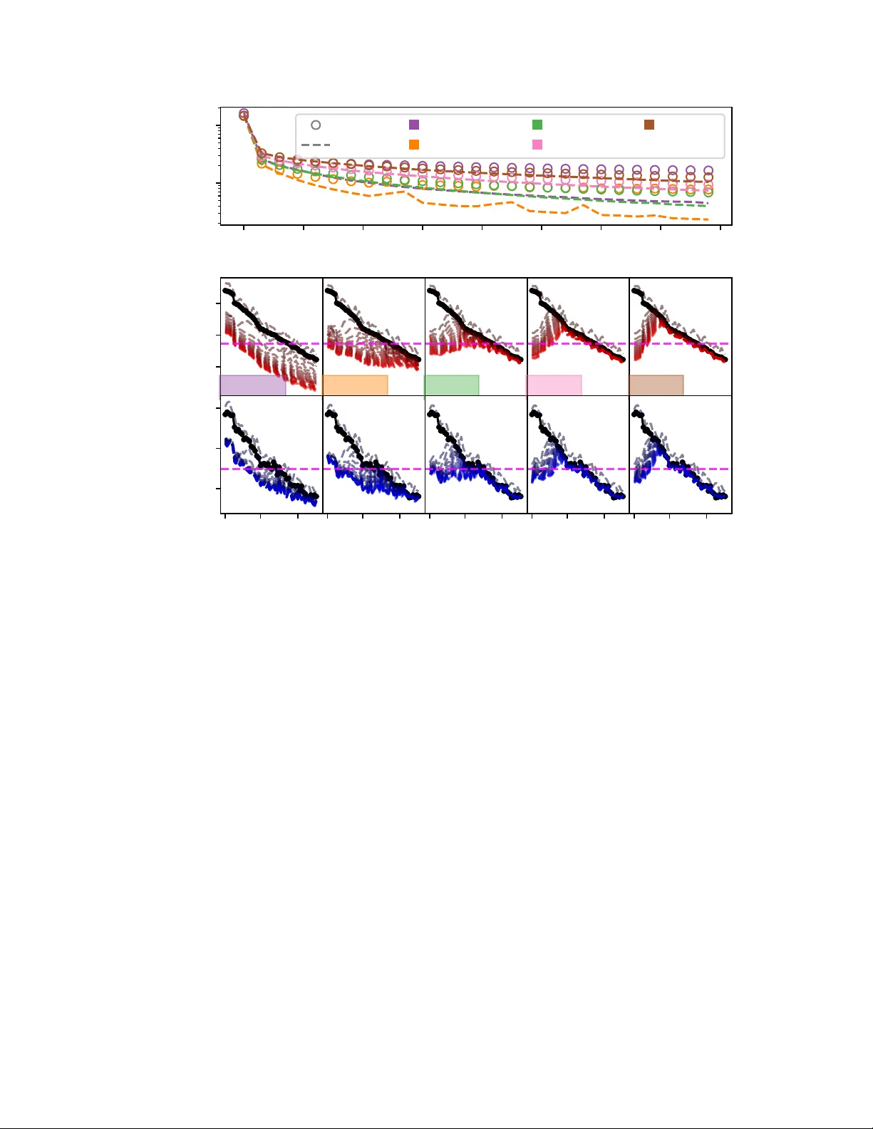
The Err or of Deep Operator Networks Is the Sum of Its P arts: Branch-T runk and Mode Err or Decompositions Alexander Heinlein Delft Institute of Applied Mathematics Delft Univ ersity of T echnology Delft, 2628CD, The Netherlands a.heinlein@tudelft.nl Johannes T araz Delft Institute of Applied Mathematics Delft Univ ersity of T echnology Delft, 2628CD, The Netherlands johannes.taraz@gmail.com Abstract Operator learning has the potential to strongly impact scientiﬁc computing by learning solution op- erators for differential equations, potentially accelerating multi-query tasks such as design optimiza- tion and uncertainty quantiﬁcation by orders of magnitude. Despite proven uni versal approximation properties, deep operator networks (DeepONets) often exhibit limited accuracy and generalization in practice, which hinders their adoption. Understanding these limitations is therefore crucial for further advancing the approach. This work analyzes performance limitations of the classical DeepONet architecture. It is shown that the approximation error is dominated by the branch network when the internal dimension is sufﬁciently lar ge, and that the learned trunk basis can often be replaced by classical basis functions without a signiﬁcant impact on performance. T o in vestigate this further, a modiﬁed DeepONet is constructed in which the trunk network is re- placed by the left singular vectors of the training solution matrix. This modiﬁcation yields sev eral key insights. First, a spectral bias in the branch network is observed, with coefﬁcients of dominant, low-frequenc y modes learned more effecti vely . Second, due to singular-v alue scaling of the branch coefﬁcients, the o verall branch error is dominated by modes with intermediate singular v alues rather than the smallest ones. Third, using a shared branch network for all mode coefﬁcients, as in the standard architecture, improv es generalization of small modes compared to a stacked architecture in which coef ﬁcients are computed separately . Finally , strong and detrimental coupling between modes in parameter space is identiﬁed. 1 Introduction Operator learning Many systems in science and engineering can be formulated using dif ferential equations, and a large body of research e xists on solving them ef ﬁciently and accurately . This work focuses on approximating the time e volution operator of time-dependent partial differential equations (PDEs), which maps the initial condition to the solution at a later time. Classical numerical methods (e.g., ﬁnite elements with time-stepping) ef ﬁciently compute solutions for individual initial conditions but offer no ef ﬁcient way to approximate the entire operator , as each initial condition requires repeated integration. Approximating solution operators is crucial for tasks such as PDE-constrained optimization [1, 2] and uncertainty quantiﬁcation [3]. Operator learning (OL) methods directly approximate mappings between function spaces using neural networks [4, 5, 6], complementing classical reduced order modeling (R OM) [7, 8]. OL is central to scientiﬁc machine learning, combining techniques from scientiﬁc computing and machine learning [9]. Deep operator networks (DeepONets) Building on theoretical results by Chen and Chen [10], Lu et al. [4] in- troduced DeepONets, which have become a standard architecture for operator learning. The DeepONet consists of two sub-networks: the trunk network outputs N basis functions ev aluated at coordinate x , and the branch network Preprint. Under re view . Branc h net (co eﬃcien ts) Input function p b 1 ( p ) b 2 ( p ) . . . b N ( p ) t 1 ( x ) t 2 ( x ) . . . t N ( x ) T runk net (basis functions) x Ev aluation co ordinate P N i =1 t i ( x ) b i ( p ) Input function p Branc h net b 1 ( p ) b 2 ( p ) . . . b N ( p ) T runk matrix T = Φ 1 Σ 1 P N i =1 σ i ϕ i b i ( p ) 10 50 90 inner dimension N 10 − 2 10 − 1 10 0 relativ e errors total error = branch err or + trunk error 1 20 40 mo de index i 10 1 10 2 10 3 10 4 w eighted mode loss σ 2 i L i base initial ﬁnal branch error = P N i =1 σ 2 i L i Figure 1: V isualizations of the standard DeepONet (top left) and this work’ s main contrib utions: the decomposition into trunk and branch error (top right) and the modiﬁed DeepONet’ s architecture (bottom left) which allo ws us to further inv estigate the dominant branch error via the mode loss decomposition (bottom right). The visualizations of the architectures are adapted and reproduced from [4]. outputs coef ﬁcients for these basis functions given a sampled initial condition. The output is a linear combination of trunk basis functions with branch coefﬁcients. The architecture is visualized in ﬁg. 1 (top left). Despite theoretical guarantees, DeepONets face practical limitations including high training data demands and limited generalizabil- ity . V arious modiﬁcations have been proposed; for a comprehensive overvie w see [11]. Some notable modiﬁcations are K olmogorov-Arnold-DeepONets [12], improved architectures [13], two-step training with trunk orthogonaliza- tion [14], and multi-ﬁdelity training [15, 16, 17]. Other operator learning approaches Other OL approaches include learning Green’ s functions for interpretable solutions of linear PDEs [18, 19, 20, 21], and addressing resolution dependence through Fourier neural operators [22, 5], con volutional neural operators [6, 23, 24], and Laplace neural operators [25]. Additionally , there are theoretical in vestig ations of errors [26, 27, 14, 28] in DeepONets and other neural operator architectures. Physics-informed neural networks (PINNs) [29, 30, 31] form another pillar of scientiﬁc ML, and can be combined with DeepONets [32, 33, 34, 35, 36, 37, 38]. Related work Our work is inspired by the theoretical w ork by Lanthaler et al. [27] analyzing DeepONet error . Moreov er , in section 6, we use a modiﬁed DeepONet: the trunk network is replaced by ﬁxed basis vectors deriv ed from the singular value decomposition (SVD) of the training data matrix, as this basis captures most of the variance in the data. This is (up to a scaling with the singular values and a whitening of the data) very similar to the POD- DeepONet [39] and the SVD-DeepONet [40]. In addition, the ﬁxed basis functions studied in section 5 are similar to the spectral neural operator [41], and ﬁxed bases (for input and output) are also used in the principal component analysis (PCA) neural operator [3, 42]. Beyond PCA, using the bases from nonlinear methods, such as kernel-PCA, for OL has been in vestigated in [43]. A direct comparison between DeepONets and ROM and their combination has been studied in [44], by training a DeepONet to learn the residual of a classical ROM. Related to our study of the 2 DeepONet’ s projection error is the inv estigation of the basis functions learned by a DeepONet and their use for a spectral method in [45]. In this work, we also inv estigate spectral bias [46], i.e., the tendency of neural networks to learn low-frequenc y components faster than high-frequency ones. While previous works, such as [47, 48, 49, 50, 51], examine spectral bias in the spatial dependency , our inv estigation focuses on spectral bias in the branch network, which captures the input function dependency . Additionally , by comparing the unstacked and stacked DeepONets [4] (i.e., the architectural coupling of the modes), we establish a connection to the ﬁeld of multi-task learning (MTL) [52]. Lastly , just as we exploit the speciﬁc DeepONet structure to decompose the error and gain insight into the network’ s inner workings, [53] le verage this same structure to de v elop a more efﬁcient optimization algorithm. Outline Section 3 describes the DeepONet architecture, training/testing setup, and data. In section 4, we decompose the error into trunk and branch components. Section 5 in vestigates the trunk network by replacing learned basis functions with ﬁxed bases, showing that branch error dominates for large N (cf. ﬁg. 1 (top right)). In section 6, we modify the DeepONet with a ﬁxed SVD basis, enabling mode loss decomposition. W e ﬁnd that intermediate modes contribute signiﬁcantly to branch error (cf. ﬁg. 1 (bottom right)) and observ e spectral bias in the branch netw ork for advection-dif fusion, KdV , and Burgers’ equations. This rev eals, on the one hand, the improv ed generalization through parameter sharing, and on the other hand, the detrimental coupling between modes in DeepONets trained with gradient descent. Furthermore, Adam mitigates gradient imbalance across singular v alue scales. Section 7 concludes with discussion and limitations. T able 1 contains notation. T o summarize, our three main contributions are: 1. W e systematically study trunk and branch errors with respect to the inner dimension N for practical examples. 2. W e decompose the branch error into modes, sho wing signiﬁcant contrib utions of the intermediate modes. 3. The decomposition enables analysis of spectral bias in the branch netw ork and mode coupling effects. The code and data from this study are av ailable at https://github.com/jotaraz/ ModeDecomposition- DeepONets . 2 Glossary symbol name note Z + Moore–Penrose in verse of matrix Z ran ( Z ) range / column space of matrix Z || Z || F Frobenius norm || Z || F : = q P ij Z 2 ij N number of output neurons of branch and trunk net (“inner dimen- sion”) N ∈ N eq. (3) X spatial domain of interest X ⊂ R d sec. 3.2 C ( X ) set of continuous functions on X u solution function of time-dependent PDE u ∈ C ( X × [0 , τ ]) sec. 3.2 p input function (e.g., initial condition of time-dependent PDE), later also used for discretized input function p ( · ) = u ( · , t = 0) ∈ C ( X ) sec. 3.2 τ ev olution time p ( · ) 7→ u ( · , τ ) sec. 3.2 m number of input functions in a data set m ∈ N sec. 3.4 M number of sampling points of p M ∈ N sec. 3.3 ¯ x j j -th sampling point of p with 1 ≤ j ≤ M ¯ x j ∈ X sec. 3.3 ˆ p discretized input function (sampled at ¯ x j ), later p is used to de- note this too ˆ p ∈ R M sec. 3.3 G true solution operator G : p ( · ) 7→ u ( · , t = τ ) sec. 3.2 ˜ G θ approximation of G (using a DeepONet) sec. 3.2 x coordinate at which G ( p )( · ) and ˜ G θ ( ˆ p )( · ) are ev aluated x ∈ X n number of coordinates to ev aluate G ( p )( · ) and ˜ G θ ( ˆ p )( · ) in test and training data n ∈ N sec. 3.4 A target data matrix A ∈ R n × m sec. 3.4 t k k -th trunk output neuron: either a function t k ( x ) or a vector t k = ( t k ( x 1 ) . . . t k ( x n )) T t k ∈ C ( X ) or t k ∈ R n sec. 3.3 T trunk output matrix T ik = t k ( x i ) , T ∈ R n × N sec. 3.4 3 b k k -th branch output neuron: either a function b k ( p ) or a vector b k = ( b k ( p 1 ) . . . b k ( p m )) T b k ∈ C  R M  or b k ∈ R m sec. 3.3 B branch output matrix B j k = b k ( p j ) , B ∈ R m × N sec. 3.4 ˜ A approximation of A by the DeepONet ˜ A = T B T ∈ R n × m sec. 3.4 ε squared total error of DeepONet approximation ε : = || A − ˜ A || 2 F sec. 4.2 δ relati ve error of DeepONet approximation δ := √ ε/ || A || F X tr training variant of a v ariable X (e.g., X = ε, A, ... ) X te test variant of a v ariable X σ k k -th singular value of A tr (ordered descendingly) Σ = diag ( σ 1 , . . . , σ r ) eq. (5) ϕ k k -th mode / k -th left singular vector of A tr ϕ k ∈ R n , Φ = [ ϕ 1 . . . ϕ r ] eq. (5) v k optimal coefﬁcients for the k -th mode and the training data’ s in- put functions / k -th right singular vector of A tr v k ∈ R m tr , V = [ v 1 . . . v r ] eq. (5) w k optimal coefﬁcients for the k -th mode and the test data’ s input functions w k ∈ R m te L loss / mean-squared error of DeepONet approximation ε/ ( nm ) L k,tr unweighted training loss of mode k || b k,tr − v k || 2 2 eq. (8) L k,te unweighted test loss of mode k (normalized for comparability to L k,tr ) m tr m te || b k,te − w k || 2 2 eq. (9) σ 2 k L k weighted loss of mode k sec. 6.2 – unweighted base loss / mode loss L k for b k = 0 1 (train), m tr m te || w k || 2 2 (test) sec. 6.2 – weighted base loss / mode loss σ 2 k L k for b k = 0 σ 2 k (train), σ 2 k m tr m te || w k || 2 2 (test) sec. 6.2 T able 1: Notation frequently used in this work. 3 Background and Setup This section provides background on neural networks, the problem setup (time e v olution under a PDE), the DeepONet architecture, and the training/testing framew ork. 3.1 F oundations of Neural Networks and Machine Learning This section provides a self-contained overvie w of foundational concepts in neural networks and optimization algo- rithms used to train them. Consider approximating a function f using a parametric model ˜ f θ with parameters θ . Giv en inputs { x 1 , ..., x m } and target outputs { y 1 , ..., y m } with y i = f ( x i ) , training ﬁnds optimal parameters θ opt ∈ arg min θ m X i =1 | y i − ˜ f θ ( x i ) | 2 , minimizing the mean-squared error (training loss) L tr ( θ ) = 1 m m X i =1 | y i − ˜ f θ ( x i ) | 2 . (1) 3.1.1 Neural Networks By the universal approximation theorem [54, 55], neural netw orks can approximate continuous functions. A one-layer network models ˜ f θ ( x ) = N X k =1 θ ( out ) k σ   ϑ ( W, 1) k  T x + ϑ ( B , 1) k  = θ ( out ) H θ (1) ( x ) , where H θ (1) ( x ) : = σ   ϑ ( W, 1)  T x + ϑ ( B , 1)  is the hidden layer with parameters θ (1) =  ϑ ( W, 1) , ϑ ( B , 1)  , and σ is a non-polynomial activ ation function. Each term σ   ϑ ( W, 1) k  T x + ϑ ( B , 1) k  in this sum is called a neur on . Multi- layer perceptrons (MLPs) apply D hidden layers successively: z 1 = H θ (1) ( x ) , z 2 = H θ (2) ( z 1 ) , etc., with output 4 ˜ f θ ( x ) = θ ( out ) z D . The parameters are θ =  θ (1) , θ (2) , . . . , θ ( D ) , θ ( out )  . (2) This composition is done because, in practice, it reduces the number of necessary parameters for a giv en accuracy [56], compared with a perceptron with a single hidden layer . The number of hidden layers D is called depth, hence the term deep learning for neural networks with multiple hidden layers. The number of neurons in one layer is often called the width of this layer . If all layers have the same width, this is referred to as the neural netw ork’ s hidden layer width w . W e use GELU acti vation [57]: σ ( x ) = GE LU ( x ) := x 2  1 + erf  x √ 2  . 3.1.2 Optimization Schemes Gradient descent (GD) updates parameters θ t iterativ ely: θ t +1 = θ t − α t ∇L tr ( θ t ) , where α t is the learning rate [58, 59]. Ho wev er , GD often con v erges slo wly or gets trapped in local minima. Adam [60] combines momentum [61] and adaptiv e learning rates [62, 63]. The update θ t +1 = θ t + δ θ t uses: m t = β 1 m t − 1 + (1 − β 1 ) ∇L tr ( θ t ) , v t = β 2 v t − 1 + (1 − β 2 )( ∇L tr ( θ t )) 2 , ˆ m t = m t 1 − β t 1 , ˆ v t = v t 1 − β t 2 , δ θ t = − α t ˆ m t √ ˆ v t + ¯ ϵ + ϵ . The learning rate α t may follow a schedule (e.g., constant or exponential decay). Unless stated otherwise, we use Adam. Hyperparameters are listed in section A. 3.2 General Problem Setup Consider the time-dependent PDE on spatial domain X ⊂ R d and time interval (0 , τ ] : ∂ u ∂ t = D ( u ) , in X × (0 , τ ] , B ( u ) = 0 , on ∂ X × (0 , τ ] , u ( · , 0) = p ( · ) , in X , where D is a (possibly nonlinear) differential operator, B denotes a suitable boundary condition on ∂ X , and p ∈ C ( X ) is the initial condition. Under appropriate regularity assumptions on X , D , B , and p , this PDE admits a unique solution u ∈ C ( X × [0 , τ ]) . W e then deﬁne the time ev olution (or solution) operator G : C ( X ) → C ( X ) , p ( · ) 7→ u ( · , τ ) , which maps the initial condition to the solution at time τ . Remark 1 . The function p plays multiple roles: it is the initial condition of the PDE, the input to the solution operator G , and the function that parametrizes the solution. Correspondingly , the operator learning literature uses the terms initial condition, input function, and parameter function interchangeably . W e adopt input function throughout this work. 3.3 DeepONet The DeepONet, as introduced in [4], is designed to approximate such solution operators. It can be seen as a deep neural network realization of the architecture in the generalized universal approximation theorem for operators in [10]. T o make the inﬁnite dimensional problem, that is, mapping p ( · ) ∈ C ( X ) to u ( · , τ ) ∈ C ( X ) , computationally accessible, the initial condition p is encoded in a ﬁnite dimensional v ector space as ˆ p = ( p ( ¯ x 1 ) . . . p ( ¯ x M )) T ∈ R M by sampling at M locations. This potentially in v olves a loss of information, which we will also address in section 3.4. As mentioned brieﬂy before, the DeepONet is a neural network consisting of two sub-networks: the trunk network outputs t k ( x ) giv en coordinate x , and the branch network outputs b k ( ˆ p ) given ˆ p . The ﬁnal output is ˜ G θ ( ˆ p )( x ) = N X k =1 b k ( ˆ p ) t k ( x ) , (3) 5 where θ are parameters and N is the number of output neurons of both trunk and branch network; see also ﬁg. 1 (top left). Equi valently , the DeepONet’ s output is a linear combination of the N trunk output neurons t k ( x ) with the branch network’ s output neurons b k ( ˆ p ) as coefﬁcients. Thus, all DeepONet output functions ˜ G θ ( ˆ p )( · ) lie in the trunk space T ( N ) : = span { t k } N k =1 ⊂ C ( X ) . The dimension of T ( N ) is at most N , with equality when the trunk functions { t k } N k =1 are linearly independent; in practice, this is typically the case. For simplicity , we call N the inner dimension of the DeepONet and we denote the trunk functions as basis functions. Both trunk and branch network are usually implemented as MLPs, but other choices are possible, as previously men- tioned. W e focus on this standard architecture with MLP-based designs; analyzing more advanced DeepONet v ariants is left to future work. The parameters of both sub-networks together form θ , the DeepONet’ s parameters. These are found by minimizing the mean-squared loss L ( θ ) = 1 K K X i =1 | G ( p i )( x i ) − ˜ G θ ( ˆ p i )( x i ) | 2 , ov er K samples of input functions p i and ev aluation coordinates x i . 3.4 Setup f or T raining and T esting Our setup uses: 1. Initial conditions from a low-dimensional subspace with sufﬁcient sampling ( M lar ge) such that p is recon- structible from ˆ p . For simplicity , we thus stop distinguishing between p and ˆ p (details in section B). 2. Discretization with m initial conditions ( p j ) j =1 ,...,m and n ev aluation coordinates ( x i ) i =1 ,...,n , yielding K = nm training points, i.e., the full tensor product of these discretizations. 3. Same ev aluation coordinates for training and testing ( n tr = n te = n ), focusing on generalization in parameter space. W e arrange the targets (or true solutions) in a matrix A ij = G ( p j )( x i ) , such that A ∈ R n × m . The DeepONet output is ˜ A ij = ˜ G θ ( p j )( x i ) = N X k =1 t k ( x i ) b k ( p j ) ⇐ ⇒ ˜ A = T B T , where T ik = t k ( x i ) ∈ R n × N and B j k = b k ( p j ) ∈ R m × N are trunk and branch outputs. The loss is L ( θ ) = 1 K || A − ˜ A || 2 F with Frobenius norm || Z || 2 F = P ij z 2 ij . This matrix notation simpliﬁes analysis and enables efﬁcient computation by ev aluating T once for all inputs. 3.5 Data and Experiments In this work, we train DeepONets to approximate the time evolution operators that map the initial condition to the solution at a giv en ﬁnal time τ . Our standard example problem is the KdV equation, similar to [45], 0 = ∂ u ∂ t + u 2 π ∂ u ∂ x + 0 . 01 8 π 3 ∂ 3 u ∂ x 3 ∀ x ∈ (0 , 1) , t > 0 , ∂ 2 u ∂ x 2 (0 , t ) = ∂ 2 u ∂ x 2 (1 , t ) ∀ t ≥ 0 , u (0 , t ) = u (1 , t ) ∀ t ≥ 0 , u ( x, t = 0) = p ( x ) ∀ x ∈ (0 , 1) , ∂ u ∂ x (0 , t ) = ∂ u ∂ x (1 , t ) ∀ t ≥ 0 , p ( x ) = 5 X k =1 a k sin(2 π k x ) ∀ x ∈ (0 , 1) , with τ = 0 . 2 . Most results shown in this work are computed for this standard example. W e also consider the advection-dif fusion equation and Burgers’ equation, training separate operators for each PDE and value of τ . Unless stated otherwise, the observations reported apply qualitati vely to all e xample problems described in section C; in general, we report results only for the KdV equation and include additional examples when they offer ne w insights or qualitativ e dif ferences. 6 4 Error Decomposition Into T runk and Branch Errors In this section, we deﬁne the projection error and formalize how the total approximation error is distributed between trunk and branch. As mentioned in section 3.4, we consider a ﬁxed ev aluation grid for the trunk network as this simpliﬁes the further discussion. Thus, we no w use the terms basis functions and basis vectors (obtained through the ev aluation of the basis functions on the grid) interchangeably . 4.1 Projection Err or Consider a set of vectors { a i } m i =1 ⊂ R n and a basis { t k } N k =1 ⊂ R n . The error of projecting { a i } m i =1 onto the space spanned by { t k } N k =1 ⊂ R n , or the pr ojection err or , quantiﬁes ho w well the a i can be reconstructed through optimal linear combinations of the t k . For accurate reconstruction, this error should be small. More formally , we deﬁne the projection error as ε P ( T , A ) := || ( I − T T + ) A || 2 F , where T = [ t 1 . . . t N ] ∈ R n × N , A = [ a 1 . . . a m ] ∈ R n × m , and T + denotes the Moore-Penrose in verse of T . Here, T T + represents the orthogonal projection onto the span of the { t k } N k =1 . Thus, ( I − T T + ) A captures the part of A that cannot be represented by the t k [64]. 4.2 T runk and Branch Errors W e adapt the error decomposition frame work of Lanthaler et al. [27] with two simpliﬁcations: we eliminate the encoding error by ensuring p can be reconstructed from ˆ p (cf. section 3.4), and we deﬁne the error o ver a ﬁnite sample set rather than a probability measure ov er the input space. This allows for a more direct analysis of how the total approximation error splits between trunk and branch networks. W e consider the dif ference between the DeepONet’ s output ˜ A and the target data matrix A : ˜ A − A = T B T − A = T B T − T T + A + T T + A − A = T ( B T − T + A ) + ( T T + − I ) A. Since T ( B T − T + A ) and ( T T + − I ) A are orthogonal to each other , this yields the error decomposition ε := || ˜ A − A || 2 F = || T ( B T − T + A ) || 2 F | {z } =: ε B + || ( T T + − I ) A || 2 F | {z } =: ε T = ε P ( T ,A ) . (4) In the following sections, we in vestigate the dif ferent error components ε B and ε T . 4.2.1 T runk Error Equation (4) thus deﬁnes the trunk error ε T as the projection error ε P ( T , A ) with the trunk matrix T , that is, the error of projecting the target data matrix onto the trunk space, cf. section 3.3. This formally proves that a small projection error is necessary for a small error ε , but in general, not sufﬁcient. No w , we consider the SVD of the training data matrix A = ΦΣ V T = [Φ 1 Φ 2 ]  Σ 1 0 0 Σ 2   V T 1 V T 2  = Φ 1 Σ 1 V T 1 + Φ 2 Σ 2 V T 2 , (5) with Φ 1 ∈ R n × N , Σ 1 ∈ R N × N and V 1 ∈ R m × N . Then, the Eckart-Y oung-Mirsky theorem [65] states that the projection error for all matrices T ∈ R n × N satisﬁes ε P ( T , A ) ≥ || Σ 2 || 2 F , with equality achie ved by T = Φ 1 C for any full-rank matrix C ∈ R N × N . Intuitiv ely , this is because the ﬁrst N left singular vectors of A capture the N principal directions of A , that is, the N directions with the highest variance. 4.2.2 Branch Error T o better understand the branch error ε B , we ﬁrst compute the branch matrix B ∗ , which is optimal in the following sense: gi ven a trunk matrix T , B ∗ is the branch matrix for which T B T best approximates A in the Frobenius norm. B ∗ = arg min B ∈ R m × N || A − T B T || 2 F = arg min B ∈ R m × N || ( I − T T + ) A + T T + A − T B T || 2 F = arg min B ∈ R m × N  || ( I − T T + ) A || 2 F + || T ( T + A − B T ) || 2 F  = arg min B ∈ R m × N || T ( T + A − B T ) || 2 F = ( T + A ) T . 7 10 50 90 10 − 2 10 − 1 10 0 relativ e error δ 10 50 90 δ δ T δ B Learned SVD Leg. Cheb. Cos inner dimension N Figure 2: Relativ e total, trunk and branch errors of DeepONets with various bases plotted over N . Colors: Purple lines: learned trunk (standard DeepONet), orange: SVD basis, green: Legendre polynomials, pink: Chebyshev polynomials, brown: cosine. Line-symbols: T otal error δ (circle), trunk error δ T (dashed), branch error δ B (solid). The relativ e error is deﬁned in the glossary , table 1. Thus, when in vestig ating the branch network, one might intuiti vely deﬁne the branch error as ε C := || B − B ∗ || 2 F = || B − ( T + A ) T || 2 F = || B T − T + A || 2 F , (6) that is, the difference between the actual branch matrix B and the optimal branch matrix B ∗ . The inequality ε ≤ || T || 2 2 || B T − T + A || 2 F | {z } ε C + || ( T T + − I ) A || 2 F (7) can be deriv ed as a bound on ε . While ε C puts the same weight on the error of each branch neuron, ε B = || T ( B T − T + A ) || 2 F accounts for the trunk matrix T , weighting the approximation error of each branch neuron (column of B ) by the norm of the corresponding trunk neuron. Hence, we use ε B as the branch error . Remark 2 . In practice, eq. (7) is a very loose bound, since the norms of the trunk neurons v ary strongly , cf. section D. 5 In v estigating the T runk Network The error decomposition enables systematic in vestigation of the trunk network. Many trunk modiﬁcations e xist: orthogonalization [14], Fourier features [39], SVD basis [3, 39], Chebyshev or trigonometric functions [41], and transfer learning [45]. W e in vestigate: (1) Ho w do prescribed bases compare to learned bases? (2) Does the learned trunk approach optimal trunk error? (3) Ho w is the error distributed between trunk and branch? W e compare dif ferent bases t k , either learned or prescribed, b ut the output remains P N k =1 t k ( x ) b k ( p ) . W e test (details in section E): Learned (standard DeepONet), SVD ( t k is k -th left singular vector of A ), Le gendre ( k -th Legendre polynomial), Chebyshev ( k -th Chebyshev polynomial), Cosine ( t k ( x ) = cos(( k − 1) π x ) ). Figure 2 shows errors for different bases. For small N , learned and SVD bases perform best. The learned basis plateaus around N = 20 , while SVD error decreases slowly . Legendre and Chebyshev errors decrease until N = 70 , then increase. For large N , cosine achiev es lo west total error . Across examples, all bases match or exceed learned basis performance for large N . The SVD basis achie ves the lowest trunk error on training data by the Eckart-Y oung-Mirsk y theorem [65]. Figure 2 shows empirically that this translates to the test data as well (see section G for further discussion). Howe ver , optimal projection error doesn’t guarantee optimal total error – low branch error is also necessary . For large N , trunk errors become negligible for all bases. This implies, in particular, that the standard DeepONet learns trunk functions spanning the solutions. 8 The non-negligible total error for lar ge N implies signiﬁcant branch error , which increases with N . For Legendre and Chebyshev , this causes total error to increase. Intuitiv ely , approximating 10 coefﬁcients is easier than 90. Motiv ated by this, we study branch errors in detail next. 6 In v estigating the Branch Network In section 5, we observed that, for our examples and large N , the branch error dominates (i.e., the coefﬁcient approx- imation is poor). In this section, we study whether all coefﬁcients are poorly approximated or only those for certain basis vectors, and why . T o this end, we introduce the DeepONet with the ﬁxed SVD basis in section 6.1. In section 6.2, we decompose the branch error into individual coefﬁcient errors, which we also refer to as mode losses. Next, in sec- tion 6.3, we analyze the distribution of the mode losses in practice. Lastly , in section 6.4, we study phenomena that affect the coef ﬁcient error distrib ution, such as spectral bias and inter -coefﬁcient coupling. 6.1 Modiﬁed DeepONet matrix formulation individual evaluation true solution (train)  Φ 1 Σ 1 V T 1 + Φ 2 Σ 2 V T 2  ij = P r k =1 σ k ( ϕ k ) i ( v k ) j true solution (test)  Φ 1 Σ 1 W T 1 + Φ 2 Σ 2 W T 2  ij = P r k =1 σ k ( ϕ k ) i ( w k ) j stand. DeepONet  T B T  ij = P N k =1 t k ( x i ) b k ( p j ) mod. DeepONet  Φ 1 Σ 1 B T  ij = P N k =1 σ k ( ϕ k ) i b k ( p j ) T able 2: Comparison of true solution (train/test), modiﬁed DeepONet and standard DeepONet in matrix formulation and for indi vidual e v aluation at coordinate x i and initial condition p j . The rank of the data matrix is denoted as r . For better comparison to the modiﬁed DeepONet, the SVD of the true solution is displayed. In this section, we modify the DeepONet by replacing the trunk netw ork by the SVD basis. This modiﬁed DeepONet is used for the remainder of the work to in v estigate the branch network’ s error . This facilitates the analysis signiﬁcantly , since it reduces the DeepONet parameters to the branch network parameters. As discussed in section 4.2.1, for any full rank matrix C , the trunk matrix T = Φ 1 C , with Φ 1 chosen as the left singular v ectors, minimizes the trunk error , which we call the SVD basis. W e in vestig ate this case here, using C = Σ 1 as a scaling, which corresponds to t k = σ k ϕ k for the k -th output neuron. W e moti vate this choice in section F. In table 2, we compare the true solution for test and training data, the modiﬁed DeepONet, and the standard DeepONet, we show their matrix formulations (center column), and the output for individual coordinates and individual input functions (right column). This shows that the optimal branch matrix for the modiﬁed DeepONet is V 1 , i.e., the matrix containing the right singular vectors. As this will be relev ant in section 6.4.1, it is important to note that this is equiv alent to stating that, for the initial condition p j , the k -th branch output neuron is trained to predict V j k . The neural network architecture of the modiﬁed DeepONet is visualized in ﬁg. 1 (bottom left). For the sake of simplicity in notation, we use the term DeepONet to refer to the modiﬁed DeepONet (with the SVD basis scaled with the singular values) for the remainder of this work. When we use the term standard DeepONet , we mean a DeepONet with a learned trunk basis. Additionally , we call the left-singular vectors ϕ i the modes from no w on. 6.2 Mode Decomposition of the Branch Error W e decompose the (modiﬁed) DeepONet’ s training error by applying eq. (4) and, using the SVD of the training data matrix A tr and the resulting orthogonality , split it into trunk and branch components. The branch error , which measures the total coefﬁcient approximation error , then further decomposes into individual mode losses, each capturing 9 how well a single mode’ s coef ﬁcient is approximated: A tr = Φ 1 Σ 1 V T 1 + Φ 2 Σ 2 V T 2 ε tr = || ˜ A tr − A tr || 2 F = || Φ 1 Σ 1 B T tr − Φ 1 Σ 1 V T 1 − Φ 2 Σ 2 V T 2 || 2 F = || Φ 1 Σ 1 B T tr − Φ 1 Σ 1 V T 1 || 2 F + || Φ 2 Σ 2 V T 2 || 2 F = || Σ 1 B T tr − Σ 1 V T 1 || 2 F + || Σ 2 || 2 F = N X i =1 σ 2 i || b i,tr − v i || 2 2 | {z } =: L i,tr + || Σ 2 || 2 F (8) By design, the trunk space is spanned by the ﬁrst N left-singular vectors of A tr , so ε T = || Σ 2 || 2 F . With this choice the DeepONet achieves the optimal trunk error for the training data. Since || Σ 2 || 2 F equals the trunk error, || Σ 1 B T tr − Σ 1 V T 1 || 2 F is the branch error . Equation (8) thus shows the modiﬁcation’ s main advantage for our analysis: the branch error decomposes into errors σ 2 i L i for different modes. The unweighted mode loss L i is the dif ference between v i and b i , that is, the true coef ﬁcients of mode i and the coefﬁcients b i predicted by the DeepONet, for all input functions. Since the unweighted mode losses L i are scaled by the squared singular values σ 2 i to yield the total error ε in eq. (8), we deﬁne the weighted mode loss as σ 2 i L i . A similar error decomposition can be deriv ed for the test data. W ith w i denoting the optimal coefﬁcients to approxi- mate the test data using the training SVD basis (see section G for details), the test branch error decomposes as ε B ,te = N X i =1 σ 2 i || b i,te − w i || 2 2 . T o facilitate comparison between training and test mode losses, we deﬁne the test mode loss L i,te := m tr m te || b i,te − w i || 2 2 (9) with a normalization factor such that both losses are scaled consistently; the precise deﬁnition is gi ven in section G. Remark 3 . T o better judge whether a mode loss is low or high, we introduce the base loss . W e seek to deﬁne the base loss, such that observing a mode loss L i that exceeds its base loss indicates that the branch netw ork is ne glecting mode i . T o this end, the base loss of mode i is deﬁned as the loss for b i = 0 , i.e., when the DeepONet predicts a zero coefﬁcient for mode i . On the training data, the unweighted base loss is || v i || 2 2 = 1 because V 1 is semi-orthogonal, thus the weighted base loss is σ 2 i . For the test data, the unweighted base loss is m tr m te || w i || 2 2 ≈ 1 . Thus, the weighted base loss is σ 2 i m tr m te || w i || 2 2 . Observing a mode loss L i that exceeds its base loss means that the model performs worse than the trivial prediction b i = 0 . 6.3 Distribution of Mode Losses In this section, we in v estigate how training and test branch errors distrib ute across modes. W e in v estigate three optimization algorithms — plain GD (section 6.3.1), loss re-weighting (section 6.3.2), and Adam (section 6.3.3) — to understand their effects on mode-speciﬁc approximation quality . Throughout this analysis, we use the following terminology: Since the i -th mode is associated with singular value σ i (ordered descendingly), we refer to modes with low indices as larg e modes , modes with high indices as small modes , and those in between as intermediate modes . Here, we take large modes to be i ≲ 10 and small modes to be i ≳ 30 ; this choice is some what arbitrary b ut the moti v ation for it will become clearer throughout the discussion of the results. 6.3.1 Gradient Descent T raining W e ﬁrst examine DeepONets trained using plain GD. Figure 3 shows both the unweighted mode losses L i and the weighted mode losses σ 2 i L i for both training and test data over the course of training. The respectiv e base losses (cf. section 6.2) are shown for reference. An interesting pattern emerges: only the largest ≈ 10 modes show signiﬁcant loss reduction below their base losses during training. This creates a characteristic error distribution in the weighted mode loss, where intermediate modes (indices 12-17 in our e xamples) contrib ute most to the total error; the y are neither well-approximated like large modes nor negligible like small modes due to tiny singular values. Furthermore, the mode losses corresponding to small singular values exceed the base losses, indicating neglect through the GD optimizer . These learning dynamics are 10 1 20 40 B) unw eigh ted test loss L j 1 20 40 10 1 10 2 10 3 10 4 C) weigh ted train loss σ 2 j L j mo de index j 1 20 40 10 − 2 10 − 1 10 0 mo de loss A) unw eigh ted train loss L j base initial ﬁnal 1 20 40 D) weigh ted test loss σ 2 j L j base initial ﬁnal Figure 3: W eighted mode losses f or DeepONet trained with GD. Unweighted (A,B) and weighted (C,D) training (A,C) and test (B,D) mode losses at different training stages, colored from gray (initial) to red/blue (ﬁnal) shown as dashed lines. The respecti ve base losses are sho wn as black dot-solid lines. driv en by gradient domination from large singular values. Since the gradient of the total loss with respect to the parameters is: ∇ θ L = 1 nm N X i =1 σ 2 i ∇ θ L i , the contributions from small modes become negligible due to the σ 2 i weighting, prev enting the GD optimizer from improving their approximation e ven when their unweighted losses L i are large. Remark 4 . A related phenomenon termed gradient starvation [66, 67] has been identiﬁed in classiﬁcation with cross- entropy loss, where correctly classiﬁed samples cease contributing to the gradient, causing dominant features to pre- vent the learning of other informati v e features. While our setting dif fers (we use MSE loss where all samples continue contributing) the common thread is that gradient-based optimization can systematically ne glect certain learnable com- ponents when others dominate the gradient signal. 6.3.2 Modiﬁed Loss Re-W eighting T o address the gradient imbalance, we introduce a modiﬁed loss function with adjustable mode weighting: L e, tr = 1 nm tr N X i =1 σ 2+2 e i L i, tr , where the e xponent e controls the re-weighting: e < 0 ampliﬁes small modes, e > 0 emphasizes large modes, and e = 0 reco vers the standard loss. T o prevent gradient explosion or vanishing, we scale the learning rate by σ − 2 e 1 , keeping the largest mode’ s contribution in v ariant. W e use L e, tr only to compute gradients (and thus parameter updates), not as a performance metric. Note that the re-weighted loss for e = − 1 is equiv alent to using ε C , deﬁned in eq. (6), instead of ε B in the loss function. Figure 4 shows the effect of this re-weighting. For e = − 1 , which weights all modes equally regardless of their singular values, we achieve signiﬁcant loss reduction across all training modes. Howe ver , this comes with a critical trade-off: small modes improve dramatically in training but se verely overﬁt, with test losses near base le vels despite low training losses. In our e xperiments, the optimal balance emer ges at e = − 0 . 5 , which achie v es the lo west test error for two reasons. First, it maintains reasonable approximation quality for large modes (better than e = − 1 ). Second, it meaningfully improves intermediate and small modes (better than e ≥ 0 ). For e > 0 , the optimizer neglects small modes, with their losses e xceeding base levels, i.e., higher loss than zero coefﬁcients. Only the ﬁrst 10, 8, and 5 modes improv e for e = 0 . 0 , 0 . 5 , and 1 . 0 respectively , sho wing ho w increased emphasis on lar ge modes comes at the e xpense of all others. This analysis re v eals a fundamental insight: The standard loss function ( e = 0 ) is poorly calibrated for the multi-scale nature of the mode decomposition. The steep singular v alue decay creates an optimization landscape where gradients are dominated by a small subset of modes, leaving most of the representation capacity unused. 11 0 500 1000 1500 2000 2500 3000 3500 4000 ep o c hs 3 × 10 − 1 10 0 relativ e error δ test train e = − 1 . 0 e = − 0 . 5 e = 0 . 0 e = 0 . 5 e = 1 . 0 10 − 2 10 0 10 2 w eighted training mo de losses e = − 1 . 0 1 20 40 10 − 1 10 1 w eighted test mo de losses e = − 0 . 5 1 20 40 e = 0 . 0 1 20 40 mo de index j e = 0 . 5 1 20 40 e = 1 . 0 1 20 40 Figure 4: Model performance across different exponents e and training epochs for DeepONets trained using GD. T op panel: Relati ve error δ = || A − ˜ A || F / || A || F for both training (dashed lines) and test (circles) data across different exponents ( e = − 1 . 0 , − 0 . 5 , 0 . 0 , 0 . 5 , 1 . 0 ) ov er 4000 epochs. Center and bottom row: W eighted training (center row) and test (bottom row) mode losses at different training stages, colored from gray (initial) to red/blue (ﬁnal). Each column corresponds to a dif ferent exponent e . The third column shows the DeepONet trained using the standard loss ( e = 0 ). The plots in the center and bottom row contain the respective base losses in black, and a pink dashed horizontal line marking the maximum mode loss in the last training epoch of e = 0 , facilitating comparison between different e xponents e . 6.3.3 Adam Optimizer The Adam optimizer provides an alternati v e to the gradient imbalance problem through its adaptive learning rate mechanism. Figure 5 sho ws that Adam achie ves signiﬁcantly lo wer total losses than GD with standard weighting, and its mode loss distribution is more similar to GD with e ≈ − 0 . 5 or − 1 . 0 . Unlike GD with e = 0 , Adam reduces all training mode losses below their base values, ev en for small modes, though at different rates. The optimizer achiev es signiﬁcant loss reduction on approximately 30 modes for both training and test data, whereas GD effecti v ely improves only the ﬁrst ten. This suggests that Adam’ s per-parameter learning rate adaptation compensates for the singular value imbalance, ef fecti v ely implementing an implicit re-weighting scheme. The mode loss distribution under Adam can be characterized as follows: Large modes ( i ≲ 10 ) are well-approximated with low weighted losses. Note that Adam approximates the large modes far better than GD (cf. ﬁg. 3). Small modes ( i ≳ 30 ) contribute negligibly due to tiny singular values. The intermediate modes’ losses are signiﬁcantly improv ed compared to base losses but still contribute signiﬁcantly to the total error due to non-negligible singular values. Furthermore, note that large modes have a signiﬁcantly higher contribution to the test loss compared to the training loss. When explicitly re-weighting Adam ( e  = 0 ), we observe that e = − 1 . 0 yields approximately homogeneous unweighted mode losses L i, tr ≈ constant for the training data; this can be inferred from the weighted mode losses in section H.1, since the weighting factor σ 2 i is known. Howe ver , similar to GD, aggressiv e emphasis on 12 1 20 40 B) unw eigh ted test loss L j 1 20 40 10 1 10 2 10 3 10 4 C) weigh ted train loss σ 2 j L j mo de index j 1 20 40 10 − 3 10 − 1 mo de loss A) unw eigh ted train loss L j base initial ﬁnal 1 20 40 D) weigh ted test loss σ 2 j L j base initial ﬁnal Figure 5: W eighted mode losses f or DeepONet trained with Adam. Unweighted (A,B) and weighted (C,D) training (A,C) and test (B,D) mode losses at different training stages, colored from gray (initial) to red/blue (ﬁnal) shown as dashed lines. The respecti ve base losses are sho wn as black dot-solid lines. small modes ( e < 0 ) leads to o verﬁtting. For Adam, we observe optimal test performance at e = 0 . This indicates that Adam’ s implicit re-weighting already strikes a good balance for generalization. Remark 5 . The superior performance of adaptiv e gradient methods extends beyond Adam; for instance, AdaGrad shows similar improv ements over standard GD (see section H.2). This consistent pattern suggests that addressing the gradient imbalance through adaptiv e learning rates is crucial for operator learning tasks where the loss function admits a multi-scale decomposition. 6.4 Mechanisms Inﬂuencing the Mode Loss Distribution Having established how different optimizers affect the mode loss distrib ution, we now inv estigate the underlying mechanisms driving these patterns. W e examine three complementary perspectiv es: spectral bias in neural networks, (some) architectural design choices, and parameter-space coupling between modes. 6.4.1 Spectral Bias Spectral bias [46, 68] is the tendency of neural networks to learn low-frequenc y components faster and more accurately than high-frequency ones. W e in vestigate whether this af fects the branch network’ s mode loss distribution. Since section 5 sho ws trunk error is negligible for large N , we focus on the branch network. The modiﬁcation in section 6.1 provides well-deﬁned target functions for analysis: the j -th branch neuron predicts V kj for input p k , deﬁning the right singular function ρ j : p k 7→ V kj . If spectral bias af fects the branch, mode losses L j should correlate with ρ j frequency: high-frequency ρ j should yield higher losses. W e deﬁne the function frequency of g : R d → R using the Fourier transform F ( g )( ξ ) = R R d g ( x ) exp( − 2 π iξ T x ) dx . The mean frequency [69] is f ( g ) = R R d |F ( g )( ξ ) | 2 || ξ || 2 dξ R R d |F ( g )( ξ ) | 2 dξ . W e ﬁrst inv estigate spectral bias in the branch network on a synthetic dataset with curated spectral properties. As described in more detail in section I.1, the synthetic data is created such that the mean frequency of ρ j is f ( ρ j ) ≈  F 0 exp( α ( j − 1)) if α > 0 , F 0 exp( α ( j − 1 − N )) else . Thus, F 0 denotes the minimum frequency and α denotes the rate of increase (or decrease) of the frequencies. W e set the singular values to σ j = exp( β j ) . Since β = 0 makes the ordering of right singular vectors non-unique, we require β  = 0 . Firstly , we consider | β | small to isolate spectral bias effects from singular value weighting. For instance, β = − 0 . 01 in ﬁg. 6 (top) yields σ 2 1 /σ 2 5 ≈ 1 . 08 , so all modes are approximately equally rele vant while remaining correctly ordered. W e then compare two cases: (i) α = 0 . 2 and (ii) α = − 0 . 2 . The mode losses in both cases are very similar , and in both cases, the low-frequenc y modes have smaller mode losses. In ﬁg. 6 (bottom), we consider the same frequencies α = ± 0 . 2 , b ut β = − 0 . 5 , i.e., a strong prioritization of the ﬁrst few modes ( σ 2 1 ≈ 55 σ 2 5 ). Here, we see that despite the initially slo wer learning of the higher -frequency features, they are e ventually learned due to their higher relev ance. This illustrates the competing effects of loss weighting and spectral bias. 13 10 − 1 10 0 β = − 0 . 01 test train 0 1000 2000 10 − 1 10 0 β = − 0 . 5 0 . 25 0 . 50 0 . 75 1 . 00 0 . 25 0 . 50 0 . 75 1 . 00 10 − 3 10 − 1 10 1 initial mo de losses ﬁnal mo de losses frequency 2 4 10 − 3 10 − 1 10 1 increasing freq., α = 0 . 2 decreasing freq., α = − 0 . 2 2 4 ep o c hs relativ e error δ mo de index j un weigh ted mo de loss L j / / / / / / frequency f ( ρ j ) / / 1 Figure 6: Spectral bias in modiﬁed DeepONet f or synthetic data. Left: Relati ve error o ver epochs (training error as dashed line and test error as circles; nearly identical). Center/right: Unweighted mode losses (left scale) at different training stages (colored from black (initial) to red (ﬁnal)) with frequencies of right singular functions (right scale). The center column shows the case of increasing frequencies ( α = 0 . 2 ), and the right column shows the case of decreasing frequencies ( α = − 0 . 2 ); the corresponding relative errors are shown in purple and orange respectiv ely in the left column. T op/bottom: The top row sho ws synthetic data with singular values σ j = exp( − 0 . 01 j ) , while the bottom row has σ j = exp( − 0 . 5 j ) . W e now return to the PDE datasets (advection-diffusion, KdV , and Burgers) and in vestig ate the impact of spectral bias on the mode loss distribution. The (in verse) scaled singular values 1 /σ 0 . 2 i , the unweighted mode losses, and the frequencies f ( ρ i ) of the right singular functions ρ i are sho wn in ﬁg. 7 for the follo wing considered e xample problems: advection-dif fusion with τ = 0 . 5 , KdV with τ = 0 . 2 , KdV with τ = 0 . 6 , and Burgers with τ = 0 . 1 . T o show the trend of the frequencies of ρ i , we choose two methods to estimate the frequencies: the total variation (TV) norm and the Laplacian energy (LE). The TV norm estimates frequency by measuring how rapidly the function values change between neighboring samples, while the LE uses concepts from spectral graph theory to quantify oscillations on a graph constructed from the data. Both methods are k -nearest neighbor methods; we use k = 3 and k = 50 for the TV norm and LE, respectively . A detailed description of both methods can be found in section I.2. Note that each plot in ﬁg. 7 contains two y -axis scales, left and right, both logarithmic. For the KdV and Burgers equations (second–fourth columns in ﬁg. 7), we observe a clear correlation between f ( ρ i ) and the mode losses L i for both test and training data. Since both test and training mode losses are low for low frequencies and high for high frequencies, the branch network learns a generalizing approximation for lo w frequencies while underﬁtting high frequencies. For the advection-dif fusion equation (ﬁrst column), the estimated frequencies f ( ρ i ) v ary only weakly with i . Unlike the KdV and Burgers equations, no general trend is observable. Howe v er , we observe an approximately constant test mode loss L i,te , indicating signiﬁcant overﬁtting. Due to the different input dimensions M across the example problems, a reliable method to compare the frequencies of the ρ i between problems is not av ailable. Consequently , an explanation based on spectral bias for why the DeepONet overﬁts the advection-diffusion equation compared to other equations cannot be given. An alternative hypothesis, unrelated to spectral bias, is that the advection-diffusion problem’ s low rank (exactly 20, matching the inner dimension N ) remov es the approximation pressure present in higher-rank problems like KdV , potentially allowing the network to memorize training data without learning general- 14 10 − 1 10 0 mo de index i 1 8 16 10 − 5 10 − 4 10 − 3 10 − 2 10 − 1 10 0 un weigh ted mo de loss L i / / AD τ = 0 . 5 1 20 40 KdV τ = 0 . 2 1 20 40 KdV τ = 0 . 6 1 20 40 Burgers τ = 0 . 1 L i,tr L i,te TV LE σ − 0 . 2 i frequency and singular v alues / / / 1 Figure 7: Spectral bias in modiﬁed DeepONet for different PDEs. Unweighted training (red) and test (blue) mode losses (left scale), the frequencies (right scale) of the right singular functions ρ i estimated via the TV norm with k = 3 (green) and LE k = 50 (pink) and the scaled singular v alues σ − 0 . 2 i (black, right scale) are shown. Example pr oblems (by column): advection-dif fusion (AD) equation with τ = 0 . 5 , KdV equation with τ = 0 . 2 , KdV equation with τ = 0 . 6 and Bur gers’ equation with τ = 0 . 1 . izable structure, thus resulting in uniform overﬁtting across all modes. Ho we ver , conﬁrming this hypothesis requires further in vestig ation in future work. 6.4.2 Architectural Coupling Both the standard and the modiﬁed DeepONet, Section 6.1, use a single branch network with shared hidden layers outputting all mode coefﬁcients simultaneously . Howe ver , together with the normal (or unstacked) DeepONet, Lu et al. also proposed the so-called stacked DeepONet [4]. Instead of one multi-layer perceptron with N output neurons, the branch network in the stacked DeepONet consists of N multi-layer perceptrons with one output neuron each, see ﬁg. 8a. W e thus say that the coef ﬁcients are ar chitectur ally coupled in the unstacked DeepONet. T o inv estigate the inﬂuence of architectural coupling, we compare the performance of stacked and unstacked Deep- ONets. Speciﬁcally , we use a stacked DeepONet whose branch networks each hav e depth D = 5 and hidden layer width w sta = 42 . W e compare this to an unstacked DeepONet with the same number of trainable parameters. T o achiev e this, we choose w unst = 495 and D = 5 . Figure 8b and 8c show the total loss over training and the mode losses of the stacked and unstacked DeepONets, respectiv ely . The stack ed DeepONet achieves a lo wer training error , while the unstack ed DeepONet achieves a slightly lower test error , indicating overﬁtting in the stacked DeepONet. The mode losses show that the stacked DeepONet does not ov erﬁt uniformly across modes. F or large modes, the stacked DeepONet achieves the smallest test and training errors. Howe ver , for small modes, the stacked DeepONet’ s low training losses do not transfer to the test data. Even for intermediate modes, the unstacked network generalizes signiﬁcantly better than the stack ed DeepONet. The ﬁrst key observ ation from section 6.3 was that small modes seem to generalize poorly when ﬁtted well on training data. The stacked DeepONet experiments corroborate this hypothesis. Furthermore, we observe that unstacking, or neuron-sharing, helps ov erall generalizability but not for all modes. In particular, it seems to negati vely impact the training loss and generalizability of large modes while impro ving the generalizability of smaller modes. Remark 6 . This counterintuiti ve result connects to insights from MTL [52]. Recall that the shared hidden layers in the unstacked architecture force the netw ork to learn representations that work across multiple modes. When dif ferent tasks (here, approximating different mode coef ﬁcients) share an underlying structure, this parameter sharing acts as an implicit re gularizer , promoting sets of parameters that generalize well rather than ov erﬁtting to individual modes. This implies that ev en when practitioners require only speciﬁc modes (e.g., the coefﬁcients for speciﬁc spatial frequencies), the unstacked architecture may still be preferable. The parameter sharing facilitates learning of generalizable features that improve approximation quality for target modes, ev en if other outputs are discarded. Note that this is a different connection to MTL than works such as [70, 16, 71] draw; they train a so-called foundation model on different PDEs, while we consider multiple tasks within one PDE. 15 Input function p Branc h n e t 1 Branc h n e t 2 . . . Branc h n e t N b 1 ( p ) b 2 ( p ) . . . b N ( p ) T runk matrix T = Φ 1 Σ 1 P N j =1 σ j b j ( p ) ( ϕ j ) i (a) 0 2500 5000 7500 10000 ep o c hs 10 − 2 10 − 1 10 0 relativ e error δ test train stac ked unstac ked (b) 10 − 4 10 − 1 10 2 w eighted training mo de losses stac ked 1 20 40 10 − 2 10 0 10 2 w eighted test mo de losses unstac ked 1 20 40 mo de index j (c) Figure 8: Stacked and unstacked DeepONets. (a) Architectur e of the stacked modiﬁed DeepONet. Figure 1 (bottom left) shows the unstacked DeepONets for reference. Adapted and reproduced from [4]. (b) Relative errors for stacked and unstack ed DeepONets trained with Adam. (c) W eighted mode losses f or stacked and unstacked DeepONets trained with Adam. W eighted training (top row) and test (bottom row) mode losses at different training steps, colored from gray (initial) to red/blue (ﬁnal). Columns correspond to different architectures and hidden layer widths (left: stacked with w sta = 42 , right: unstacked with w unst = 495 ), as indicated by the labels. The center and bottom row plots also contain the respectiv e base losses in black, and a pink dashed horizontal line marking the maximum mode loss of the fully-trained unstacked DeepONet. 6.4.3 Update-Based Coupling In comparing stacked and unstacked DeepONets, we in vestigated ho w rearranging the branch network so that modes hav e separated parameters (while keeping the number of parameters constant) affects generalization. In this section, we consider unstacked DeepONets and in vestigate further how much of the loss stems from mode coupling. W e are concerned with the modes’ coupling in parameter space. Changing the v alue of the i -th branch output neuron does not change the contribution of any other mode to the DeepONet output because of the modes’ orthogonality ( ϕ T i ϕ j = 0 for i  = j ). Ho we ver , when training with gradient descent to reduce the loss for mode i , this parameter update changes all network parameters, since they are shared between modes. Thus, the mode i -speciﬁc parameter update can signiﬁcantly alter the values of all branch output neurons, not just the i -th one, due to the neuron-sharing discussed in section 6.4.2. W e no w giv e a formal deﬁnition of mode coupling in parameter space for DeepONets trained with GD. Unless stated otherwise, any loss function in this section is ev aluated at the current parameters θ , and gradients are computed with respect to θ . For clarity , we write ∇ L i instead of ∇ θ L i ( θ ) , and ∇L instead of ∇ θ L ( θ ) . Consider a GD parameter update δ θ = − α ∇L tr = − α nm tr N X j =1 σ 2 j ∇ L j,tr , where we also drop the iteration index t . Choosing a sufﬁciently small learning rate α allows us to approximate the change in the training and test loss function using a ﬁrst-order T aylor e xpansion. As we will see, the T aylor e xpansion allows us to partition the loss change into coupling and non-coupling parts. The ﬁrst-order T aylor expansion of the total loss (train or test) change ∆ L is ∆ L ≈ ( ∇L ) T δ θ = 1 nm tr N X i =1 σ 2 i ( ∇ L i ) T δ θ = − α n 2 m 2 tr N X i =1 N X j =1 σ 2 i σ 2 j ( ∇ L i ) T ∇ L j,tr = : d + Ω , 16 where d = : − α n 2 m 2 tr N X i =1 σ 4 i ( ∇ L i ) T ∇ L i,tr and Ω = : − α n 2 m 2 tr N X i =1 X j  = i σ 2 i σ 2 j ( ∇ L i ) T ∇ L j,tr . W e call d the diagonal term and Ω is the off-diagonal term . Note that d tr ≤ 0 , by deﬁnition. Then, we deﬁne the relativ e coupling strength as γ : = Ω d + Ω . Assume successful training, i.e., d + Ω < 0 , then detrimental coupling between the modes, i.e., Ω > 0 , is symbolized by γ < 0 , while beneﬁcial coupling Ω < 0 is symbolized by γ > 0 . Furthermore, training and test performance of DeepONets trained with GD have so f ar been observed to be very similar; these DeepONets are underﬁtting. W e thus only explicitly focus on discussing the results for the training data. W e can no w compute γ over the course of the training for dif ferent DeepONets. Figure 9a plots the (ne gati ve) relati v e coupling strength over the loss reduction for DeepONets of different hidden layer widths. For all hidden layer widths we ﬁnd detrimental coupling, γ < 0 . Furthermore, we ﬁnd strong decoupling with increased width; i.e., the wider DeepONets exhibit signiﬁcantly smaller negativ e coupling strengths. Note that these wider, decoupled DeepONets also achiev e lo wer test and training losses. 10 − 4 10 − 3 loss reduction − ∆ L 10 − 3 10 − 2 10 − 1 10 0 10 1 negativ e relative coupling strength − γ w = 50 w = 100 w = 220 w = 335 w = 495 (a) Negative relati ve coupling strength − γ plotted over loss reduction − ∆ L for DeepONets of differ- ent hidden-layer widths w . The ﬁgure sho ws mod- els with hidden layer widths 50 (purple), 100 (or- ange), 220 (green), 335 (pink) and 495 (brown). 10 − 1 10 1 w eighted mo de losses σ 2 j L j w = 50 w = 335 base initial ﬁnal 1 20 40 1 20 40 coupling matrix S ij 1 20 40 mo de index j (b) Mode losses and coupling matrices. T op r ow: W eighted mode losses at different training stages, colored from gray (initial) to red (ﬁ- nal). Singular values sho wn in black. Bottom row: Entries of S tr matrix after 4000 epochs. Red entries indicates a positiv e entry and blue indi- cates a negati ve entry (same colorscale for both matrices). Left / right: Hidden layer width w = 50 / w = 335 . Figure 9: Update-based coupling f or DeepONets of different hidden-layer widths. Furthermore, we can inspect the coupling directly by deﬁning the coupling matrix S ∈ R N × N with entries S ij = − α n 2 m 2 tr σ 2 i σ 2 j ( ∇ L i ) T ∇ L j,tr . Thus, d + Ω = P N i,j =1 S ij . Figure 9b shows the mode losses and the coupling matrices for DeepONets with w = 50 and w = 335 . They both share a pattern: most entries in the ﬁrst 10 ro ws and columns are positiv e (red). This means that the coupling between any two modes i, j is likely to be detrimental if i ≤ 10 . The pattern is less distinct in the wider DeepONet but still clearly visible. W e furthermore note that only the ﬁrst 10 modes’ losses are signiﬁcantly lower than their base losses; we thus refer to them (a bit euphemistically) as well-appr oximated . Thus, the coupling between a well-approximated mode and any other mode is likely to be detrimental. Howe v er , the coupling between two poorly approximated modes ( i, j > 10 ) is likely to be beneﬁcial; S ij < 0 (blue). 17 7 Conclusion and Discussion T runk and Branch Error in DeepONets W e decompose DeepONet error into trunk and branch components, adapt- ing Lanthaler et al. [27]. Across PDE examples, the branch network (learning basis coefﬁcients) dominates approxi- mation error for lar ge inner dimensions, while the trunk learns a sufﬁcient basis. T o the best of the authors’ knowledge, this is the ﬁrst empirical, systematic in vestig ation of the error distribution between basis and coef ﬁcient. Modiﬁed DeepONet with Fixed SVD Basis T o further inv estigate the branch error , we construct a modiﬁed Deep- ONet with a ﬁx ed SVD basis and brieﬂy compare it to the standard DeepONet. For simplicity , we assume the standard SVD algorithm for a full data matrix, that is, the data must be sampled on the same spatial grid for ev ery parameter conﬁguration. This is computationally intensi ve and may not be feasible in higher-dimensional spatial domains, where the number of grid points grows exponentially with the spatial dimension (curse of dimensionality), b ut facilitates our analysis. The standard DeepONet is less restrictiv e regarding its training data. Furthermore, the modiﬁed DeepONet can only be ev aluated on speciﬁc grid positions – howe ver , if interpolation is used in the trunk, the modiﬁed Deep- ONet could be ev aluated on all possible positions, similar to the standard DeepONet, though this is beyond the scope of the present work. W e believ e that our ﬁndings regarding the modiﬁed DeepONet are transferable to the standard DeepONet, since the standard DeepONet’ s trunk network learns to approximate the SVD basis. Mode Decomposition of the Branch Error Mode-speciﬁc analysis (enabled by the DeepONet modiﬁcation) re- veals poor generalization for modes with small singular v alues. Furthermore, distinct but characteristic mode loss distributions for DeepONets trained with GD and Adam can be observed. This highlights GD’ s failure to capture more than the largest fe w modes. Three complementary effects shape this distribution: Spectral bias causes large errors for high-frequency modes, though its impact on generalization remains unclear . Architectural coupling (stacked vs. unstacked) produces different mode loss distributions and generalization, connecting operator learning to multi-task learning. Update-based coupling shows network width reduces mode interactions. These effects interact: right sin- gular function frequency affects coefﬁcient learnability , while parameter sharing in unstacked architectures further impacts approximation quality and training dynamics. Practical Implications Network width is crucial for reducing mode coupling. MTL methods [72, 73] for gradient conﬂicts may address mode coupling in DeepONets. Adaptiv e optimizers (e.g., Adam) help learn beyond dominant modes, and unstacked architectures impro ve generalization through parameter sharing. T raining data SVD can inform hyperparameter choices like inner dimension. The modiﬁed DeepONet and mode-decomposition analysis provide tools for understanding and improving operator learning. Limitations and Future W ork While our analysis focuses on time ev olution operators, the error decomposition framew ork is not inherently restricted to this setting and may extend to other operator types, such as steady-state solution operators, integral operators, and parameter-to-solution maps. Open questions remain, in part due to our focus on relatively smooth PDE solutions. It is not clear how our analysis would change when the trunk error becomes more pronounced, for instance, for hyperbolic equations with discontinuous initial conditions or shock formations. Moreov er , we have only considered low-dimensional spatial problems. Future work should address these scenarios and extend the analysis to different training and testing grids through an interpolator . Additionally , extending this analysis to more advanced DeepONet variants and architectures, such as those with Fourier features or K olmogorov- Arnold networks, is an important direction for future work. Lastly , to clarify the impact of spectral bias, future work should include more example problems with v aried spectral properties and improv ed frequency estimation methods. 8 CRediT authorship contribution statement Alexander Heinlein : Conceptualization, Methodology , In vestigation, Writing - re vie w and editing, Supervision Johannes T araz : Conceptualization, Methodology , Software, V alidation, In vestig ation, Writing - original draft, Writ- ing - revie w and editing, V isualization 9 Declaration of competing interest The authors declare that they have no known competing ﬁnancial interests or personal relationships that could hav e appeared to inﬂuence the work reported in this paper . 18 10 Code a vailability statement The implementation is av ailable at https://github.com/jotaraz/ModeDecomposition- DeepONets . 11 Acknowledgments W e thank Henk Schuttelaars for conceptual discussions during the early stages of this work and for feedback on related drafts. 12 Declaration of generative AI in the manuscript pr eparation pr ocess During the preparation of this work the authors used Claude [74] for proof-reading and language re vision. After using this tool, the authors revie wed and edited the content as needed and take full responsibility for the content of the published article. References [1] T . O. de Jong, K. Shukla, M. Lazar, Deep Operator Neural Network Model Predictive Control, preprint, arXiv:2505.18008 (2025). doi:10.48550/arXiv.2505.18008 . [2] D. R. Sarkar, J. Dr go ˇ na, S. Goswami, Learning to Control PDEs with Dif ferentiable Predictive Control and T ime-Integrated Neural Operators, preprint, arXi v:2511.08992 (2025). doi:10.48550/arXiv.2511.08992 . [3] K. Bhattacharya, B. Hosseini, N. B. Ko v achki, A. M. Stuart, Model Reduction And Neural Networks For Para- metric PDEs, SMAI J. Comput. Math. 7 (2021) 121–157. doi:10.5802/smai- jcm.74 . [4] L. Lu, P . Jin, G. Pang, Z. Zhang, G. E. Karniadakis, Learning Nonlinear Operators via DeepONet Based on the Univ ersal Approximation Theorem of Operators, Nat. Mach. Intell. 3 (3) (2021) 218–229. doi:10.1038/ s42256- 021- 00302- 5 . [5] N. Ko vachki, Z. Li, B. Liu, K. Azizzadenesheli, K. Bhattacharya, A. Stuart, A. Anandkumar , Neural Operator: Learning Maps Between Function Spaces with Applications to PDEs, J. Mach. Learn. Res. 24 (89) (2023) 1–97. URL https://www.jmlr.org/papers/v24/21- 1524.html [6] B. Raoni ´ c, R. Molinaro, T . De Ryck, T . Rohner , F . Bartolucci, R. Alaifari, S. Mishra, E. de B ´ ezenac, Con volu- tional Neural Operators for Robust and Accurate Learning of PDEs, in: Adv . Neural Inf. Process. Syst., V ol. 36, 2023, pp. 77187–77200. [7] P . Benner, M. Ohlberger , A. Patera, G. Rozza, K. Urban, Model Reduction of Parametrized Systems, Springer Cham, 2017. doi:10.1007/978- 3- 319- 58786- 8 . [8] S. Chaturantabut, D. C. Sorensen, Discrete Empirical Interpolation for Nonlinear Model Reduction, in: Proceed- ings of the 48h IEEE Conference on Decision and Control (CDC), 2009, pp. 4316–4321. doi:10.1109/CDC. 2009.5400045 . [9] N. Baker , F . Alexander , T . Bremer, A. Hagber g, Y . Ke vrekidis, H. Najm, M. Parashar , A. Patra, J. Sethian, S. Wild, K. Willcox, S. Lee, W orkshop Report on Basic Research Needs for Scientiﬁc Machine Learning: Core T echnologies for Artiﬁcial Intelligence (2019). URL https://www.osti.gov/servlets/purl/1478744 [10] T . Chen, H. Chen, Universal Approximation to Nonlinear Operators by Neural Networks with Arbitrary Acti- vation Functions and Its Application to Dynamical Systems, IEEE Trans. Neural Netw . 6 (4) (1995) 911–917. doi:10.1109/72.392253 . [11] S. Liu, Y . Y u, T . Zhang, H. Liu, X. Liu, D. Meng, Architectures, V ariants, and Performance of Neural Operators: A Comparativ e Re vie w, Neurocomputing 648 (2025) 130518. doi:10.1016/j.neucom.2025.130518 . [12] D. W . Abueidda, P . Pantidis, M. E. Mobasher, DeepOKAN: Deep Operator Network Based on Kolmogoro v Arnold Networks for Mechanics Problems, preprint, arXiv:2405.19143 (2024). doi:10.48550/arXiv.2405. 19143 . [13] S. W ang, H. W ang, P . Perdikaris, Improv ed Architectures and T raining Algorithms for Deep Operator Networks, J. Sci. Comput. 92 (2022) 35. doi:10.1007/s10915- 022- 01881- 0 . [14] S. Lee, Y . Shin, On the T raining and Generalization of Deep Operator Networks, SIAM J. Sci. Comput. 46 (4) (2024) C273–C296. doi:10.1137/23M1598751 . [15] A. A. How ard, M. Perego, G. E. Karniadakis, P . Stinis, Multiﬁdelity Deep Operator Networks for Data-Driven and Physics-Informed Problems, J. Comput. Phys. 493 (2023) 112462. doi:10.1016/j.jcp.2023.112462 . 19 [16] V . Kumar , S. Goswami, K. K ontolati, M. D. Shields, G. E. Karniadakis, Synergistic Learning with Multi-T ask DeepONet for Efﬁcient PDE Problem Solving, Neural Netw . 184 (2025) 107113. doi:10.1016/j.neunet. 2024.107113 . [17] L. Lu, R. Pestourie, S. G. Johnson, G. Romano, Multiﬁdelity Deep Neural Operators for Efﬁcient Learning of Partial Differential Equations with Application to Fast In v erse Design of Nanoscale Heat Transport, preprint, arXiv:2204.06684 (2022). doi:10.48550/arXiv.2204.06684 . [18] N. Boull ´ e, C. J. Earls, A. T ownsend, Data-Driv en Discovery of Green’ s Functions with Human-Understandable Deep Learning, Sci. Rep. 12 (1) (2022). doi:10.1038/s41598- 022- 08745- 5 . [19] C. R. Gin, D. E. Shea, S. L. Brunton, J. N. K utz, DeepGreen: Deep Learning of Green’ s Functions for Nonlinear Boundary V alue Problems, Sci. Rep. 11 (2021). doi:10.1038/s41598- 021- 00773- x . [20] Q. Sun, S. Li, B. Zheng, L. Ju, X. Xu, Learning Singularity-Encoded Green’ s Functions with Application to Iterativ e Methods, preprint, arXi v:2509.11580 (2025). doi:10.48550/arXiv.2509.11580 . [21] H. Melchers, J. Prins, M. Abdelmalik, Neural Green’ s Operators for Parametric Partial Dif ferential Equations, preprint, arXiv:2406.01857 (2025). doi:10.48550/arXiv.2406.01857 . [22] Z. Li, N. K ov achki, K. Azizzadenesheli, B. Liu, K. Bhattacharya, A. Stuart, A. Anandkumar , Fourier Neural Operator for Parametric Partial Dif ferential Equations, in: International Conference on Learning Representations (ICLR), 2021. URL https://openreview.net/forum?id=c8P9NQVtmnO [23] B. Bahmani, S. Goswami, I. G. K e vrekidis, M. D. Shields, A Resolution Independent Neural Operator, preprint, arXiv:2407.13010 (2024). doi:10.48550/arXiv.2407.13010 . [24] F . Bartolucci, E. de B ´ ezenac, B. Raoni ´ c, R. Molinaro, S. Mishra, R. Alaifari, Representation Equiv alent Neural Operators: A Framework for Alias-Free Operator Learning, in: Adv . Neural Inf. Process. Syst., V ol. 36, 2023, pp. 69661–69672. [25] Q. Cao, S. Goswami, G. E. Karniadakis, Laplace Neural Operator for Solving Dif ferential Equations, Nat. Mach. Intell. 6 (6) (2024) 631–640. doi:10.1038/s42256- 024- 00844- 4 . [26] N. Boull ´ e, A. T ownsend, Chapter 3 - A Mathematical Guide to Operator Learning, in: Handbook of Numerical Analysis, V ol. 25 of Numerical Analysis Meets Machine Learning, Elsevier , 2024, pp. 83–125. doi:10.1016/ bs.hna.2024.05.003 . [27] S. Lanthaler , S. Mishra, G. E. Karniadakis, Error Estimates for DeepONets: A Deep Learning Framework in Inﬁnite Dimensions, T rans. Math. Appl. 6 (1) (2022) tnac001. doi:10.1093/imatrm/tnac001 . [28] C. Schwab, A. Stein, J. Zech, Deep Operator Network Approximation Rates for Lipschitz Operators, preprint, arXiv:2307.09835 (2023). doi:10.48550/arXiv.2307.09835 . [29] M. W . M. G. Dissanayake, N. Phan-Thien, Neural-Netw ork-Based Approximations for Solving Pa rtial Dif feren- tial Equations, Commun. Numer . Methods Eng. 10 (3) (1994) 195–201. doi:10.1002/cnm.1640100303 . [30] I. Lagaris, A. Likas, D. Fotiadis, Artiﬁcial Neural Networks for Solving Ordinary and Partial Differential Equa- tions, IEEE T rans. Neural Netw . 9 (5) (1998) 987–1000. doi:10.1109/72.712178 . [31] M. Raissi, P . Perdikaris, G. E. Karniadakis, Physics-Informed Neural Networks: A Deep Learning Frame work for Solving Forward and Inv erse Problems Inv olving Nonlinear Partial Differential Equations, J. Comput. Phys. 378 (2019) 686–707. doi:10.1016/j.jcp.2018.10.045 . [32] S. Goswami, A. Bora, Y . Y u, G. E. Karniadakis, Physics-Informed Deep Neural Operator Networks, in: Machine Learning in Modeling and Simulation, Computational Methods in Engineering & the Sciences, Springer, Cham, 2023. doi:10.1007/978- 3- 031- 36644- 4_6 . [33] S. W ang, H. W ang, P . Perdikaris, Learning the Solution Operator of Parametric Partial Dif ferential Equations with Physics-Informed DeepONets, Sci. Adv . 7 (40) (2021) eabi8605. doi:10.1126/sciadv.abi8605 . [34] R. Bischof, M. Piov ar ˇ ci, M. A. Kraus, S. Mishra, B. Bickel, HyPINO: Multi-Physics Neural Operators via HyperPINNs and the Method of Manufactured Solutions, preprint, arXiv:2509.05117 (2025). doi:10.48550/ arXiv.2509.05117 . [35] V . Grimm, A. Heinlein, A. Klawonn, Learning the Solution Operator of T wo-Dimensional Incompressible Navier-Stok es Equations Using Physics-A ware Con volutional Neural Networks, J. Comput. Phys. 535 (2025) 114027. doi:10.1016/j.jcp.2025.114027 . [36] L. Mandl, S. Goswami, L. Lambers, T . Ricken, Separable Physics-Informed DeepONet: Breaking the Curse of Dimensionality in Physics-Informed Machine Learning, Comput. Methods Appl. Mech. Eng. 434 (2025) 117586. doi:10.1016/j.cma.2024.117586 . [37] D. Nayak, S. Goswami, TI-DeepONet: Learnable Time Integration for Stable Long-T erm Extrapolation, preprint, arXiv:2505.17341 (2025). doi:10.48550/arXiv.2505.17341 . 20 [38] S. W ang, P . Perdikaris, Long-T ime Integration of Parametric Evolution Equations with Physics-Informed Deep- ONets, preprint, arXiv:2106.05384 (2021). doi:10.48550/arXiv.2106.05384 . [39] L. Lu, X. Meng, S. Cai, Z. Mao, S. Goswami, Z. Zhang, G. E. Karniadakis, A Comprehensiv e and F air Compar - ison of T wo Neural Operators (with Practical Extensions) Based on F AIR Data, Comput. Methods Appl. Mech. Eng. 393 (2022) 114778. doi:10.1016/j.cma.2022.114778 . [40] S. V enturi, T . Casey , SVD Perspectives for Augmenting DeepONet Flexibility and Interpretability, Comput. Methods Appl. Mech. Eng. 403 (2023) 115718. doi:10.1016/j.cma.2022.115718 . [41] V . S. Fanasko v , I. V . Oseledets, Spectral Neural Operators, Dokl. Math. 108 (2023) S226–S232. doi:10.1134/ S1064562423701107 . [42] S. Lanthaler , Operator Learning with PCA-Net: Upper and Lo wer Complexity Bounds, preprint, arXiv:2303.16317 (2023). doi:10.48550/arXiv.2303.16317 . [43] H. Ei v azi, S. W ittek, A. Rausch, Nonlinear Model Reduction for Operator Learning, preprint, arXi v:2403.18735 (2024). doi:10.48550/arXiv.2403.18735 . [44] N. Demo, M. T ezzele, G. Rozza, A DeepONet Multi-Fidelity Approach for Residual Learning in Reduced Order Modeling, Adv . Model. Simul. Eng. Sci. 10 (2023). doi:10.1186/s40323- 023- 00249- 9 . [45] E. W illiams, A. Howard, B. Meuris, P . Stinis, What Do Physics-Informed DeepONets Learn? Understanding and Improving Training for Scientiﬁc Computing Applications, preprint, arXi v:2411.18459 (2024). doi:10. 48550/arXiv.2411.18459 . [46] N. Rahaman, A. Baratin, D. Arpit, F . Draxler, M. Lin, F . Hamprecht, Y . Bengio, A. Courville, On the Spectral Bias of Neural Networks, in: Proc. Mach. Learn. Res., V ol. 97, 2019, pp. 5301–5310. URL https://proceedings.mlr.press/v97/rahaman19a.html [47] S. Khodakarami, V . Oommen, A. Bora, G. E. Karniadakis, Mitigating Spectral Bias in Neural Operators via High-Frequency Scaling for Physical Systems, preprint, arXiv:2503.13695 (2025). doi:10.48550/arXiv. 2503.13695 . [48] Q. Kong, C. Zou, Y . Choi, E. M. Matzel, K. Azizzadenesheli, Z. E. Ross, A. J. Rodgers, R. W . Clayton, Reducing Frequency Bias of Fourier Neural Operators in 3D Seismic W av eﬁeld Simulations Through Multi-Stage Training, preprint, arXiv:2503.02023 (2025). doi:10.48550/arXiv.2503.02023 . [49] B. W ang, L. Liu, W . Cai, Multi-Scale DeepOnet (Mscale-DeepOnet) for Mitigating Spectral Bias in Learn- ing High Frequency Operators of Oscillatory Functions, preprint, arXi v:2504.10932 (2025). doi:10.48550/ arXiv.2504.10932 . [50] E. Zhang, A. Kahana, A. Kopani ˇ c ´ akov ´ a, E. T urkel, R. Ranade, J. Pathak, G. E. Karniadakis, Blending Neural Operators and Relaxation Methods in PDE Numerical Solvers, preprint, arXiv:2208.13273 (2024). doi:10. 48550/arXiv.2208.13273 . [51] A. Sojitra, M. Dhingra, O. San, FEDONet: Fourier-Embedded DeepONet for Spectrally Accurate Operator Learning, preprint, arXiv:2509.12344 (2025). doi:10.48550/arXiv.2509.12344 . [52] S. Ruder , An Overvie w of Multi-T ask Learning in Deep Neural Networks, preprint, arXi v:1706.05098 (2017). doi:10.48550/arXiv.1706.05098 . [53] J. Choi, C.-O. Lee, M. Moon, Hybrid Least Squares/Gradient Descent Methods for DeepONets, preprint, arXiv:2508.15394 (2025). doi:10.48550/arXiv.2508.15394 . [54] G. Cybenko, Approximation by Superpositions of a Sigmoidal Function, Math. Control Signals Syst. 2 (4) (1989) 303–314. doi:10.1007/BF02551274 . [55] A. Pinkus, Approximation Theory of the MLP Model in Neural Networks, Acta Numer . 8 (1999) 143–195. doi:10.1017/S0962492900002919 . [56] Y . LeCun, Y . Bengio, G. Hinton, Deep Learning, Nature 521 (2015) 436–444. doi:10.1038/nature14539 . [57] D. Hendrycks, K. Gimpel, Gaussian Error Linear Units (GELUs), preprint, arXi v:1606.08415 (2023). doi: 10.48550/arXiv.1606.08415 . [58] Y . LeCun, L. Bottou, G. B. Orr , K.-R. M ¨ uller , Neural Netw orks: Tricks of the Trade, Springer , Berlin Heidelberg, 1998. doi:10.1007/3- 540- 49430- 8_2 . [59] S. K. K umar , On W eight Initialization in Deep Neural Netw orks, preprint, arXi v:1704.08863 (2017). doi: 10.48550/arXiv.1704.08863 . [60] D. P . Kingma, J. Ba, Adam: A Method for Stochastic Optimization, in: International Conference on Learning Representations (ICLR), 2015. URL [61] D. Rumelhart, G. Hinton, R. W illiams, Learning internal representations by error propagation, in: A. Collins, E. E. Smith (Eds.), Readings in Cogniti ve Science, Morgan Kaufmann, 1988, pp. 399–421. doi:https://doi. 21 org/10.1016/B978- 1- 4832- 1446- 7.50035- 2 . URL https://www.sciencedirect.com/science/article/pii/B9781483214467500352 [62] J. Duchi, E. Hazan, Y . Singer, Adapti ve Subgradient Methods for Online Learning and Stochastic Optimization, J. Mach. Learn. Res. 12 (61) (2011) 2121–2159. URL http://jmlr.org/papers/v12/duchi11a.html [63] G. Hinton, Lecture 6e RMSprop: Di vide the Gradient by a Running A verage of Its Recent Magnitude, accessed 21.07.2025 (2012). URL https://www.cs.toronto.edu/ ~ tijmen/csc321/slides/lecture_slides_lec6.pdf [64] G. H. Golub, C. F . V . Loan, Matrix Computations, Johns Hopkins University Press, 2013. [65] C. Eckart, G. Y oung, The Approximation of One Matrix by Another of Lo wer Rank, Psychometrika 1 (3) (1936) 211–218. doi:10.1007/BF02288367 . [66] R. T achet, M. Pezeshki, S. Shabanian, A. Courville, Y . Bengio, On the Learning Dynamics of Deep Neural Networks, preprint, arXi v:1809.06848 (2020). doi:10.48550/arXiv.1809.06848 . [67] M. Pezeshki, S.-O. Kaba, Y . Bengio, A. Courville, D. Precup, G. Lajoie, Gradient Starvation: A Learning Proclivity in Neural Netw orks, preprint, arXi v:2011.09468 (2021). doi:10.48550/arXiv.2011.09468 . [68] Z.-Q. J. Xu, Y . Zhang, Y . Xiao, T raining Behavior of Deep Neural Network in Frequency Domain, preprint, arXiv:1807.01251 (2019). doi:10.48550/arXiv.1807.01251 . [69] S. Mallat, A W a velet T our of Signal Processing, Academic Press, 2008, section 2.3.2. [70] M. Herde, B. Raoni ´ c, T . Rohner , R. K ¨ appeli, R. Molinaro, E. de B ´ ezenac, S. Mishra, Poseidon: Efﬁcient Foun- dation Models for PDEs, preprint, arXiv:2405.19101 (2024). doi:10.48550/arXiv.2405.19101 . [71] Z. Zhang, C. Moya, L. Lu, G. Lin, H. Schaeffer , DeepONet as a Multi-Operator Extrapolation Model: Distributed Pretraining with Physics-Informed Fine-T uning, preprint, arXiv:2411.07239 (2024). doi:10.48550/arXiv. 2411.07239 . [72] T . Y u, S. Kumar , A. Gupta, S. Levine, K. Hausman, C. Finn, Gradient Sur gery for Multi-T ask Learning, in: Adv . Neural Inf. Process. Syst., V ol. 33, 2020, pp. 5824–5836. [73] Z. Zhang, J. Shen, C. Cao, G. Dai, S. Zhou, Q. Zhang, S. Zhang, E. Shutov a, Proactiv e Gradient Conﬂict Mitigation in Multi-T ask Learning: A Sparse T raining Perspective, preprint, arXiv:2411.18615 (2024). doi: 10.48550/arXiv.2411.18615 . [74] Anthropic, Claude, https://www.anthropic.com (2025). [75] K. Nakamura, B. Derbel, K.-J. W on, B.-W . Hong, Learning-Rate Annealing Methods for Deep Neural Networks, Electronics 10 (16) (2021) 2029. doi:10.3390/electronics10162029 . [76] DeepMind, I. Babuschkin, K. Baumli, A. Bell, S. Bhupatiraju, J. Bruce, P . Buchlovsky , D. Budden, T . Cai, A. Clark, I. Danihelka, A. Dedieu, C. Fantacci, J. Godwin, C. Jones, R. Hemsley , T . Hennigan, M. Hessel, S. Hou, S. Kapturowski, T . Keck, I. K emaev , M. King, M. Kunesch, L. Martens, H. Merzic, V . Mikulik, T . Norman, G. Papamakarios, J. Quan, R. Ring, F . Ruiz, A. Sanchez, L. Sartran, R. Schneider , E. Sezener, S. Spencer, S. Srini v asan, M. Stanojevi ´ c, W . Stoko wiec, L. W ang, G. Zhou, F . V iola, The DeepMind J AX Ecosystem (2020). URL http://github.com/google- deepmind [77] D. Zwicker , py-pde: A Python Package for Solving Partial Dif ferential Equations, J. Open Source Softw . 5 (48) (2020) 2158. doi:10.21105/joss.02158 . [78] M. Abramowitz, I. A. Stegun, Handbook of Mathematical Functions with Formulas, Graphs, and Mathematical T ables, Dov er , Ne w Y ork, 1972, section 22.5.49 and 22.5.47. [79] C. Bishop, Neural Netw orks for Pattern Recognition, Oxford Uni versity Press, 1995. [80] T . Hastie, R. T ibshirani, J. Friedman, The Elements of Statistical Learning, Springer , 2009. [81] Y . Hu, R. Xian, Q. W u, Q. Fan, L. Y in, H. Zhao, Revisiting Scalarization in Multi-T ask Learning: A Theoretical Perspectiv e, preprint, arXi v:2308.13985 (2023). doi:10.48550/arXiv.2308.13985 . [82] L. Huang, J. Qin, Y . Zhou, F . Zhu, L. Liu, L. Shao, Normalization T echniques in T raining DNNs: Methodology, Analysis and Application, IEEE Trans. Pattern Anal. Mach. Intell. 45 (8) (2023) 10173–10196. doi:10.1109/ TPAMI.2023.3250241 . [83] Z.-Q. J. Xu, Y . Zhang, T . Luo, Y . Xiao, Z. Ma, Frequency Principle: F ourier Analysis Sheds Light on Deep Neural Networks, Commun. Comput. Phys. 28 (5) (2020) 1746–1767. doi:10.4208/cicp.oa- 2020- 0085 . [84] L. I. Rudin, S. Osher, E. Fatemi, Nonlinear T otal V ariation Based Noise Remov al Algorithms, Physica D 60 (1) (1992) 259–268. doi:10.1016/0167- 2789(92)90242- F . [85] P . Getreuer , Rudin-Osher-Fatemi T otal V ariation Denoising Using Split Bregman, Image Process. Line 2 (2012) 74–95. doi:10.5201/ipol.2012.g- tvd . 22 [86] D. Spielman, Spectral and Algebraic Graph Theory, Y ale Lecture Notes, 2025. URL http://cs- www.cs.yale.edu/homes/spielman/sagt/ [87] T . Cover , P . Hart, Nearest Neighbor Pattern Classiﬁcation, IEEE T rans. Inf. Theory 13 (1) (1967) 21–27. doi: 10.1109/TIT.1967.1053964 . A A ppendix: Hyperparameters The hyperparameters used in this work are similar to those employed in related works [4, 39, 45], balancing accuracy and cost. W e use coarse hyperparameter search to maintain generality . Main ﬁndings (branch error dominance, mode loss distribution) remain qualitatively consistent across tested ranges: learning rates [10 − 4 , 8 × 10 − 3 ] , depths 3-10, widths 50-500, and different initializations. The initial learning rate α 1 = 10 − 4 , used throughout section 6.4.3, is chosen such that the ﬁrst-order T aylor expansion of the loss change approximates the true loss change ∆ L . For e very optimizer and e v ery initial learning rate α 1 , the learning rate after t epochs, α t , is giv en as α t = 0 . 95 ⌊ t/ 500 ⌋ · α 1 . This is a common schedule in machine learning [75]. The Adam parameters are chosen following [76]: β 1 = 0 . 9 , β 2 = 0 . 999 , ϵ = 10 − 8 , ¯ ϵ = 0 . T able 3 lists hyperparameters for all ﬁgures. var1 : α 1 = 10 − 4 σ − 2 e 1 (see section 6.3.2). var2 , var3 : varying values for ﬁg. 7 (AD: N = 20 , w = 332 ; KdV : N = 50 , w = 335 ; Burgers: N = 20 , w = 337 ). ﬁgure example pr ob . optimizer α 1 depth width N number of epochs 1 KdV τ = 0 . 2 Adam 2 × 10 − 3 5 100 5000 2 KdV τ = 0 . 2 Adam 2 × 10 − 3 5 100 5000 3 KdV τ = 0 . 2 GD 10 − 4 5 335 50 4000 4 KdV τ = 0 . 2 GD var1 5 335 50 4000 5 KdV τ = 0 . 2 Adam 10 − 4 5 335 50 4000 6 synth. data Adam 2 × 10 − 3 5 50 5 2000 7 Adam 10 − 4 5 var2 var3 4000 8 KdV τ = 0 . 2 Adam 10 − 4 5 50 4000 9 KdV τ = 0 . 2 GD 10 − 4 5 50 4000 10 KdV τ = 0 . 2 Adam 10 − 4 5 335 50 4000 11 KdV τ = 0 . 2 10 − 4 5 335 50 4000 T able 3: Hyperparameters of DeepONets and SVDONets used in each ﬁgure. A cell i s left empty , if there are mul- tiple DeepONets shown in the ﬁgure and it is apparent which hyperparameter values correspond to which DeepONet. The term var x denotes a varying value for the different DeepONets which is not apparent from the ﬁgure. Each var x is explained in the te xt of this section. B A ppendix: Input Function Encoding T o eliminate encoding error [27], we restrict input functions to an L -dimensional subspace: p ( x ) = P L i =1 a i sin( iπ x ) ∈ span { sin( iπ x ) } L i =1 ⊂ C ([0 , 1]) . Sampling on uniform mesh with M interior points ¯ x j = j M +1 yields ˆ p = Ψ a ∈ R M , where Ψ j i = sin( iπ ¯ x j ) and a ∈ R L . For M ≥ L , Ψ has full column rank, so coefﬁcients recov er exactly as a = Ψ + ˆ p , yielding zero encoding error . C A ppendix: Data For each example problem, the training and test data sets contain 900 and 100 input functions, respecti vely , both drawn from the same distribution. The input functions are of the form p ( x ) = L X i =1 a i sin( ω i x ) , a i ∼ U ([ − 1 , 1]) , 23 with problem-speciﬁc parameters summarized in table 4. problem L ω i τ solver n M rank ( A tr ) AD 20 2 π i 0.5, 1.0 FD + RK [77] 200 200 20 KdV 5 2 π i 0.2, 0.6, 1.0 FD + RK [77] 400 400 400 Burgers 5 π i 0.1, 1.0 spectral (100 basis) + Euler 200 50 100 T able 4: Data generation parameters for the three example problems. Here, L is the number of input function modes, ω i the corresponding frequencies, and FD + RK denotes the ﬁnite-difference method combined with a Runge–Kutta method. The PDEs and boundary conditions for the KdV equation are giv en in section 3.5; the advection-diffusion (AD) and Burgers equations follo w the same structure with the dif ferential operators and boundary conditions speciﬁed belo w . The AD equation is ∂ t u + 4 2 π ∂ x u − 0 . 01 4 π 2 ∂ 2 x u = 0 with periodic boundary conditions on (0 , 1) . Burgers’ equation is ∂ t u + u ∂ x u − 0 . 01 ∂ 2 x u = 0 with homogeneous Dirichlet boundary conditions on (0 , 1) . Range of test and training data matrices. For the AD equation, the solution operator is linear , so A tr and A te share the same 20 -dimensional range and have rank 20 . For the KdV equation; rank ( A tr ) = 400 equals the spatial dimension n , the standard basis vectors of R 400 span ran ( A tr ) , implying ran ( A te ) ⊂ ran ( A tr ) . For Burgers’ equation, the span of the discretized spectral basis functions equals the range of both data matrices. These containment properties are used in section G. Note that for the AD equation, the input functions must be sampled at M ≥ 2 L interior meshpoints. D A ppendix: Bound on the Branch Error As discussed in section 4.2.2 one can deriv e the follo wing bound on the branch error . ε B ≤ || T || 2 2 || B T − T + A || 2 F = || T || 2 2 ε C =: ε D T able 5 sho ws the dif ferent error components, and the ratio between ε B and ε D for dif ferent N . Recall that, if ε D were a tight bound on ε B , the ratio w ould be ≈ 1 , i.e., log 10 ( ε D,te /ε B ,te ) ≈ 0 . Note that the ratio increases as N increases, since the coefﬁcients of more and more basis functions are poorly approximated. N log 10 ε te log 10 ε T ,te log 10 ε B ,te log 10 ε D,te log 10 ( ε D,te /ε B ,te ) 2 4.31 4.31 0.43 0.61 0.18 10 3.26 3.24 2.05 3.34 1.30 18 2.86 2.61 2.5 4.29 1.79 50 2.59 1.62 2.54 8.29 5.75 90 2.63 -0.31 2.63 13.48 10.86 T able 5: T otal error , trunk error , branch error, upper bound on branch error ε D = || T || 2 2 ε C , and the ratio ε D /ε B . E A ppendix: Bases W e deﬁne the bases used in section 5. Except for the SVD basis vectors, all bases are f amilies of functions { t k } N k =1 ⊂ C ([0 , 1]) . For the SVD basis, the k -th trunk network output is the k -th left singular vector of the training data matrix A , i.e., t k = ϕ k ∈ R n . The learned basis functions are the trunk network outputs of a standard DeepONet. For the Legendre polynomials, we set t k ( x ) = P k − 1 (2 x − 1) . Here P k is the k -th Legendre polynomial, for instance, P 0 ( x ) = 1 , P 1 ( x ) = x, P 2 ( x ) = (3 x 2 − 1) / 2 . . . [78]. For the Chebyshe v polynomials, we set t k ( x ) = T k − 1 (2 x − 1) . Here T k is the k -th Chebyshev polynomial, for example, T 0 ( x ) = 1 , T 1 ( x ) = x, T 2 ( x ) = 2 x 2 − 1 . . . [78]. For the cosine harmonics, we set t k ( x ) = cos(( k − 1) π x ) . 24 F A ppendix: Motivation f or DeepONet Modiﬁcation W e choose T = Φ 1 Σ 1 for three reasons: (1) Φ 1 giv es optimal rank- N approximation ( ε T = || Σ 2 || 2 F ); (2) using Σ 1 makes branch targets semi-orthogonal ( || v i || 2 2 = 1 ), a common normalization in machine learning [79, 80, 81, 82]; (3) simpliﬁes analysis with straightforward unweighted mode loss L i . G A ppendix: Deriving the Mode-Based Err or Decomposition f or T est Data Since ran ( A te ) ⊂ ran ( A tr ) , we hav e A te = ΦΣ W T with W = (Σ + Φ T A te ) T . Partitioning W = [ W 1 W 2 ] yields A te = Φ 1 Σ 1 W T 1 + Φ 2 Σ 2 W T 2 , where W 1 = (Σ − 1 1 Φ T 1 A te ) T contains optimal coefﬁcients. The test error decomposes as ε te = || Σ 1 B T te − Σ 1 W T 1 || 2 F + || Σ 2 W T 2 || 2 F = N X i =1 σ 2 i || b i,te − w i || 2 2 + || Σ 2 W T 2 || 2 F . Note: A te = ΦΣ W T is not an SVD, so Φ 1 lacks optimality for test data. Unlike training ( V 1 , V 2 semi-orthogonal), W 1 , W 2 are not semi-orthogonal, so test trunk error could exceed training trunk error . Howe ver , this doesn’t occur for our examples (see table 6). problem log 10 δ T ,tr log 10 δ T ,te log 10 δ T ,tr log 10 δ T ,te log 10 δ T ,tr log 10 δ T ,te N = 10 N = 10 N = 15 N = 15 N = 20 N = 20 AD τ = 0 . 5 -0.41 -0.41 -0.78 -0.78 -12.6 -12.6 AD τ = 1 . 0 -0.69 -0.69 -1.32 -1.32 -13.1 -13.1 N = 30 N = 30 N = 50 N = 50 N = 70 N = 70 KdV τ = 0 . 2 -1.48 -1.46 -2.19 -2.10 -2.94 -2.84 KdV τ = 0 . 6 -1.04 -1.03 -1.90 -1.88 -2.71 -2.59 KdV τ = 1 . 0 -1.00 -0.99 -1.91 -1.93 -2.70 -2.70 Burgers τ = 0 . 1 -1.36 -1.29 -1.90 -1.75 -2.42 -2.20 Burgers τ = 1 . 0 -3.56 -3.35 -5.53 -5.10 -7.54 -6.75 T able 6: Relative training and test trunk errors δ T for all example problems (advection diffusion (AD), K ortewe g-de Vries (KdV) and Burgers) and v arious N . Furthermore, since the trunk error is determined by the choice of N , it can be omitted from the loss used in the neural network training. Thus, we use L tr : = 1 n tr m tr || Σ 1 B T tr − Σ 1 V T 1 || 2 F = 1 n tr m tr ε B ,tr , L te : = 1 n te m te || Σ 1 B T te − Σ 1 W T 1 || 2 F = 1 n te m te ε B ,te , as training and test loss for the modiﬁed DeepONet. This corresponds to only measuring the branch error, not the full approximation error of the matrix A . This implies L tr = 1 nm tr N X i =1 σ 2 i L i,tr , L te = 1 nm te N X i =1 σ 2 i l i . T o facilitate the comparison between the unweighted mode losses for test and training data we deﬁne the unweighted test loss of mode i as L i,te = m tr m te l i = m tr m te || b i,te − w i || 2 2 . This implies L te = 1 nm tr N X i =1 σ 2 i L i,te . Thus, the unweighted test base loss is m tr m te || w i || 2 2 . H A ppendix: Further Optimization Algorithms H.1 Re-W eighting with Adam Figure 10 shows the relati ve error and the weighted mode losses for DeepONets trained using Adam with dif ferent exponents e . 25 0 500 1000 1500 2000 2500 3000 3500 4000 ep o c hs 10 − 1 10 0 relativ e error δ test train e = − 1 . 0 e = − 0 . 5 e = 0 . 0 e = 0 . 5 e = 1 . 0 10 − 3 10 − 1 10 1 w eighted training mo de losses e = − 1 . 0 1 20 40 10 − 2 10 0 10 2 w eighted test mo de losses e = − 0 . 5 1 20 40 e = 0 . 0 1 20 40 e = 0 . 5 1 20 40 e = 1 . 0 1 20 40 mo de index j Figure 10: Model performance across different exponents e and training epochs for modiﬁed DeepONets trained using Adam. Layout and parameters identical to ﬁg. 4, with Adam replacing GD. T op panel: Rela- tiv e error δ = || A − ˜ A || F / || A || F for both training (dashed lines) and test (circles) data across different exponents ( e = − 1 . 0 , − 0 . 5 , 0 . 0 , 0 . 5 , 1 . 0 ) over 4000 epochs. Center and bottom row: W eighted training (center row) and test (bottom ro w) mode losses at different training steps, colored from gray (initial) to red/blue (ﬁnal). Each column corre- sponds to a different e xponent e . The third column shows the DeepONet trained using the standard loss ( e = 0 ). The center and bottom ro w plots also contain the respecti ve base losses in black, and a pink dashed horizontal line marking the maximum mode loss in the last training epoch of e = 0 , facilitating comparison between different e xponents e . H.2 AdaGrad Figure 11 shows the weighted mode losses for DeepONets trained with GD, Adam and AdaGrad in comparison. W e observe that both the ov erall and the mode speciﬁc test loss of the two DeepONets trained with Adam and AdaGrad are very similar . I A ppendix: Spectral Bias In this section, we provide more information on our spectral bias analysis. The generation of the synthetic data, used in section 6.4.1 to analyze spectral bias in the branch network for data with curated spectral properties, is described in section I.1. The methods to estimate the frequency of the right singular functions for the PDE-derived data is described in section I.2. In section I.2.4 these methods are e valuated on the synthetic data. I.1 Synthetic Data f or Spectral Bias A prototypical multiv ariate function g k : R M → R with mean frequency f = ∥ k ∥ 2 is g k ( p ) = sin(2 π k T p ) . W e w ould ideally set the right singular functions to ρ j = g f j z for a f amily of frequencies { f j } N j =1 and a unit vector z ∈ R M , b ut 26 0 500 1000 1500 2000 2500 3000 3500 4000 ep o c hs 10 − 1 10 0 relativ e error δ test train Adam AdaGrad GD 10 − 2 10 0 10 2 w eighted training mo de losses Adam 1 20 40 10 − 1 10 1 w eighted test mo de losses AdaGrad 1 20 40 GD 1 20 40 mo de index j Figure 11: Model perf ormance for DeepONets trained with different optimizers. T op panel: Relative error δ = || A − ˜ A || F / || A || F for both training (dashed lines) and test (circles) data for different optimizers (purple: Adam, orange: AdaGrad, green: GD) over 4000 epochs. Center and bottom row: W eighted training (center row) and test (bottom row) mode losses at dif ferent training steps, colored from gray (initial) to red/blue (ﬁnal). The center and bottom row plots also contain the respectiv e base losses in black, and a pink dashed horizontal line marking the maximum mode loss in the last training epoch of the DeepONet trained with GD, facilitating comparison between different algorithms. the resulting vectors are not necessarily orthogonal. W e address this by (1) choosing p ∈ R M and direction vectors such that the resulting vectors are approximately orthogonal, and (2) applying Gram–Schmidt orthogonalization. Algorithm 1 contains the pseudocode. The algorithm generates m sample points concentrated near the 1 M = (1 . . . 1) T direction, then constructs a sinusoidal candidate sin(2 π f j d T x ) for each frequency f j using randomly sampled directions d ∼ N ( 1 M , I M ) . Candidates are accepted only if their inner product with all previously selected functions is belo w a threshold of t = 0 . 05 , with up to K attempts per frequency . A ﬁnal Gram–Schmidt step enforces orthogonality of the basis V = [ v 1 , . . . , v N ] . Since there are no truly reliable methods to quantify the frequency of a multiv ariate function (see section I.2), we estimate the mean frequenc y of ρ j to be f j . I.2 Frequency Estimation f or Multi variate Functions W e seek to characterize the spectrum of ρ k : p j ∈ R M 7→ V j k ∈ R , which is only av ailable through samples ρ k ( p j ) = V j k . Since ρ k has multi-dimensional input sampled at irregular locations, computing its Fourier transform directly is infeasible [83]. W e employ three methods: the total variation (TV) norm [84, 85], the Laplacian energy (LE) [86], and Fourier transforms of projected data [83], described in sections I.2.1 to I.2.3. Both the TV norm and LE rely on a k -nearest neighbors algorithm ( k denotes the number of neighbors in this context). For ease of notation, we call the outputs of all methods frequencies, although the TV norm and LE technically compute related quantities. T o compare these methods, we use the relative frequency f i / (max j f j ) . Since we are primarily interested in qualitativ e trends – whether f ( ρ k ) increases or decreases with k – rather than exact values, this comparison is meaningful, as 27 Algorithm 1 Generation of right singular functions with prescribed frequencies Require: Number of trials K , desired frequencies F = { f 1 , . . . , f N } , number of samples m , input dimension M ▷ Generate sample points in R M 1: f or i = 1 to m do 2: Draw a ∼ U ([0 , 1]) and b ∼ U ([ − 1 , 1] M ) 3: x i ← a ( 1 M + 0 . 1 b ) 4: end f or 5: X ← { x i } m i =1 6: Set inner -product threshold t ← 0 . 05 ▷ Construct frequency-speciﬁc orthogonal functions 7: f or j = 1 to N do 8: for k = 1 to K do 9: Draw direction d ∼ N ( 1 M , I M ) 10: Deﬁne w i ← sin(2 π f j d ⊤ x i ) for all i = 1 , . . . , m 11: w ← [ w 1 , . . . , w m ] ⊤ 12: if max 1 ≤ a

Original Paper

Loading high-quality paper...

Comments & Academic Discussion

Loading comments...

Original Paper

Related Papers

Comments & Academic Discussion

Leave a Comment