LightSim: A Lightweight Cell Transmission Model Simulator for Traffic Signal Control Research

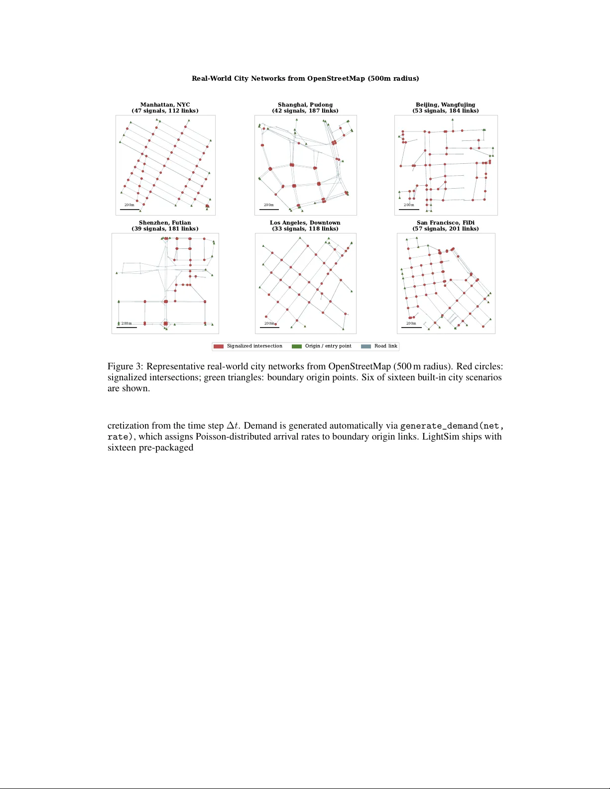
LightSim: A Lightweight Cell T ransmission Model Simulator f or T raffic Signal Contr ol Research Haoran Su New Y ork Uni versity haoran.su@nyu.edu Hanxiao Deng UC Berkeley hxdeng@berkeley.edu Abstract Reinforcement learning for traffic signal control is bottleneck ed by simulators: training in SUMO takes hours, reproducing results often requires days of platform- specific setup, and the slow iteration cycle discourages the multi-seed experiments that rigorous ev aluation demands. Much of this cost is unnecessary—for signal timing optimization, the relev ant dynamics are queue formation and discharge, which the Cell Transmission Model (CTM) captures exactly as a macroscopic flo w model. W e introduce LightSim , a pure-Python, pip-installable traffic simulator with Gymnasium and PettingZoo interfaces that runs over 20,000 steps/s on a single CPU. Across cross-simulator experiments spanning single intersections, grid networks, arterial corridors, and six real-world city networks from OpenStreetMap, LightSim preserves controller rankings from SUMO for both classical and RL strategies while training 3 – 7 × faster . LightSim is released as an open-source benchmark with nineteen b uilt-in scenarios, se ven controllers, and full RL pipelines, lowering the barrier to signal control research from days to minutes. 1 Introduction T raffic signal control is a fundamental problem in urban transportation, directly affecting congestion, emissions, and trav el time for millions of commuters daily . Reinforcement learning has emerged as a promising paradigm for adapti ve signal control, with numerous methods demonstrating improv ements ov er fixed-time and actuated controllers in simulation [W ei et al., 2018, 2019a, Chen et al., 2020, Oroojlooy et al., 2020]. Ho wever , nearly all RL-based traffic signal control research relies on microscopic traffic simulators— primarily SUMO [Lopez et al., 2018] and CityFlow [Zhang et al., 2019]. While these simulators provide high-fidelity v ehicle-lev el dynamics, they introduce substantial ov erhead for RL research: • Installation complexity . SUMO requires platform-specific binaries and en vironment vari- ables; CityFlow requires C++ compilation. Neither is pip-installable. • Configuration burden. Both require XML network files, route definitions, and detector configurations—a high barrier for RL researchers unfamiliar with transportation engineering. • Simulation speed. Inter-process communication (IPC) between Python RL code and external simulator processes creates a bottleneck, particularly for on-policy algorithms requiring many en vironment interactions. • Reproducibility . Different SUMO versions, netw ork file formats, and platform-dependent behaviors mak e exact reproduction of published results dif ficult [W ei et al., 2021]. W e observe that for the specific problem of signal timing optimization , the dominant factor is the queuing dynamics at intersections—how vehicles accumulate during red phases and discharge during Preprint. green phases. The Cell T ransmission Model (CTM) [Daganzo, 1994, 1995], a well-established macroscopic traf fic flo w model, captures precisely these dynamics while operating on aggregate densities rather than indi vidual vehicles. This makes CTM both computationally efficient and theoretically grounded: it is the exact Godunov discretization of the L WR partial dif ferential equation [Lighthill and Whitham, 1955, Richards, 1956]. Based on this insight, we present LightSim , a lightweight traffic signal simulator designed specifically for RL research. LightSim makes the follo wing contributions: 1. A fast, pure-Python simulator built on the CTM that achiev es 800 × to 21 , 000 × real-time speedup across network sizes from 1 to 64 intersections, with no external dependencies beyond NumPy . 2. Standard RL interfaces via Gymnasium [T owers et al., 2024] for single-agent and Petting- Zoo [T erry et al., 2021] for multi-agent settings, with pluggable observation, action, and rew ard components. 3. Built-in benchmarks comprising three scalable network generators, sixteen real-world city scenarios from OpenStreetMap across four continents, se ven baseline controllers, and reproducible ev aluation scripts. 4. Fidelity validation showing that LightSim’ s CTM dynamics exactly reproduce the theo- retical triangular fundamental diagram and that the relati ve performance ranking of signal controllers is preserved between LightSim and SUMO. 5. Mesoscopic extensions —start-up lost time and stochastic demand—that are backward- compatible (disabled by default) and close the fidelity gap with microscopic simulators, enabling realistic ev aluation of switching-cost-sensitive controllers. LightSim is open-source (MIT license), pip-installable ( pip install lightsim ), and requires only three lines of code to create a training en vironment: import lightsim env = lightsim.make("single-intersection-v0") obs, info = env.reset() 2 Related W ork T raffic simulators for RL. SUMO [Lopez et al., 2018] is the most widely used open-source traffic simulator , providing microscopic car-follo wing and lane-changing dynamics. CityFlow [Zhang et al., 2019] was de veloped specifically for RL-based signal control research, achieving higher throughput than SUMO through a C++ engine with a Python API. Flo w [W u et al., 2021, V initsky et al., 2018] provides a frame work wrapping SUMO for mixed-autonomy traf fic RL research. All three simulators model indi vidual vehicles and require either external binaries (SUMO, CityFlow) or comple x build toolchains. LightSim takes a fundamentally dif ferent approach: rather than simplifying the interface to a microscopic simulator , it uses a macroscopic traffic model that directly captures the queuing phenomena relev ant to signal control. Cell T ransmission Model. The CTM was introduced by Daganzo [1994] as a discrete approxima- tion to the L WR kinematic wav e model [Lighthill and Whitham, 1955, Richards, 1956] and extended to general networks by Daganzo [1995]. The CTM represents traf fic as a continuum fluid with density and flow v ariables on road cells, gov erned by the triangular fundamental diagram. It has been exten- si vely validated for macroscopic traf fic dynamics and is widely used in transportation engineering for network modeling and signal optimization [T reiber and Kesting, 2013]. T o our kno wledge, LightSim is the first implementation that packages the CTM as a standard RL en vironment with Gymnasium and PettingZoo interfaces. Signal control methods. Classical signal control includes W ebster’ s optimal fixed-time splits [W ebster, 1958], self-organizing traffic lights (SO TL) [Gershenson, 2005], and MaxPressure [V araiya, 2013], which selects the phase with maximum upstream–do wnstream queue difference and is prov ably throughput-optimal under certain conditions. RL-based approaches include IntelliLight [W ei et al., 2018], PressLight [W ei et al., 2019a] (MaxPressure-inspired rewards for arterial coordination), 2 CoLight [W ei et al., 2019b] (network-le vel cooperation via attention), and methods scaling to thousands of intersections [Chen et al., 2020]. Oroojlooy et al. [2020] used attention mechanisms for generalizable policies; Zheng et al. [2019] proposed learning phase structures. Beyond standard signal control, RL has also been applied to emergency vehicle scenarios: EMVLight [Su et al., 2022] uses decentralized RL for emergenc y vehicle passage, and Su [2026] extends this to dynamic queue-jump lane and corridor formation using hierarchical GNNs. Recent surveys [W ei et al., 2021] note that the lack of standardized benchmarks and reproducibility tools remains a major obstacle. LightSim addresses this by providing a complete, self-contained benchmark en vironment with sev en built-in controllers. 3 LightSim 3.1 Cell T ransmission Model LightSim’ s traf fic dynamics are go verned by the Cell T ransmission Model with a triangular fundamen- tal diagram. Each road link is discretized into cells of length ∆ x = v f · ∆ t , where v f is the free-flo w speed and ∆ t is the simulation time step. This discretization satisfies the Courant–Friedrichs–Lewy (CFL) condition, ensuring numerical stability . The state of each cell i at time t is characterized by its density k i ( t ) (vehicles per meter per lane). The flow between adjacent cells is determined by the sending and r eceiving functions: S i ( k ) = min( v f · k i , Q ) · ℓ i (1) R i ( k ) = min( Q, w · ( k j − k i )) · ℓ i (2) where Q is the per -lane capacity (veh/s), w is the backward w ave speed, k j is the jam density , and ℓ i is the number of lanes. The sending function represents the maximum flow a cell can emit; the receiving function represents the maximum flo w a cell can accept. The actual intra-link flow from cell i to its downstream neighbor i + 1 is: q i → i +1 = min( S i , R i +1 ) · ∆ t (3) At signalized intersections, movements connect the last cell of an incoming link to the first cell of an outgoing link. Each movement m has a turn ratio β m and saturation rate s m . The intersection flow is modulated by a binary signal mask σ m ∈ { 0 , 1 } : q m = min( β m · S from · σ m , s m , R to ) · ∆ t (4) When multiple mov ements feed the same downstream cell or draw from the same upstream cell, proportional scaling ensures conservation of v ehicles (merge and di ver ge resolution). The density update follows directly from conserv ation: k i ( t + ∆ t ) = k i ( t ) + 1 ∆ x · ℓ i X in q in − X out q out ! (5) Figure 1 illustrates the CTM mechanics: (a) a road link discretized into cells with density values, (b) the sending–receiving flo w computation between adjacent cells, and (c) how signal phases modulate flows at an intersection. 3.2 Architecture and API Figure 2 shows LightSim’ s modular architecture. The system is organized into three layers: Core engine. The simulation engine operates on a compiled network —a set of flat NumPy arrays deri ved from the logical network topology . Link properties (free-flow speed, wav e speed, jam density , capacity , lanes) and cell connectivity (upstream/downstream indices) are stored as contiguous arrays, enabling vectorized computation of sending flows, recei ving flows, and density updates in a single pass. The signal manager tracks per-node phase states, green timers, and yellow/all-red intervals, producing a mov ement mask each step. RL en vironments. LightSim provides two en vironment interfaces: 3 ( a ) C e l l D i s c r e t i z a t i o n ∆ x = v f · ∆ t k = 0 . 0 2 Cell 1 k = 0 . 0 4 Cell 2 k = 0 . 0 8 Cell 3 k = 0 . 1 2 Cell 4 k = 0 . 0 5 Cell 5 Link (road segment) ( b ) S e n d i n g & R e c e i v i n g F l o w s C e l l i C e l l i + 1 S i = m i n ( v f k i , Q ) · ` i R i + 1 = m i n ( Q , w ( k j − k i + 1 ) ) · ` q = m i n ( S i , R i + 1 ) · ∆ t Flow = min(supply , demand) ( c ) S i g n a l - C o n t r o l l e d I n t e r s e c t i o n P 0 GREEN RED RED GREEN σ m ∈ © 0 , 1 ª S N E W Figure 1: Cell T ransmission Model mechanics. (a) A road link is discretized into cells, each storing aggregate density k (color indicates congestion lev el). (b) Flow between cells is the minimum of the upstream sending flow S i and downstream receiving flo w R i +1 . (c) At signalized intersections, a binary signal mask σ m controls which mov ements recei ve green; the phase alternates between NS (green) and EW (red) in this example. Core Engine Network CTM Flow Model Signal Manager Demand Manager RL En vironments Gymnasium (single-agent) PettingZoo (multi-agent) Obs / Act / Rew ard User Interface lightsim.make() Scenarios Registry Benchmarks + Baselines W eb V isualization OSM Import Figure 2: LightSim architecture. The core engine implements CTM flow dynamics, signal man- agement, and demand injection using v ectorized NumPy operations. RL en vironments wrap the engine with standard Gymnasium/PettingZoo interf aces. Users interact through a high-le vel API with built-in scenarios, benchmarks, a web visualization dashboard, and OpenStreetMap network import. • LightSimEnv (Gymnasium): single-agent control of one signalized intersection. The agent selects from n phases each decision step (ev ery k simulation steps). • LightSimParallelEnv (PettingZoo): multi-agent control where each signalized intersec- tion is an independent agent acting in parallel. Both interfaces support pluggable components registered by name: observations ( default , pressure , full_density ), actions ( phase_select , next_or_stay ), and rewards ( queue , pressure , delay , throughput ). The default observ ation concatenates a one-hot encoding of the current phase, normalized incoming link densities, and binary queue indicators; the queue rew ard returns the neg ative total queue on incoming links, a standard choice in the literature [W ei et al., 2021]. Network generators. LightSim includes generators for common topologies: N × M grids, lin- ear arterial corridors, and single intersections. Networks can also be loaded from JSON defini- tions or imported from OpenStreetMap. The OSM import pipeline provides a high-level API— from_osm_point(lat, lon, dist) —that downloads the road network within a giv en radius, automatically identifies signalized intersections from OSM tags (or by node degree as a f allback), gen- erates mo vements at both signalized and unsignalized intersections, and computes CFL-stable cell dis- 4 200m Manhattan, NY C (47 signals, 112 links) 200m Shanghai, Pudong (42 signals, 187 links) 200m Beijing, W angfujing (53 signals, 184 links) 200m Shenzhen, F utian (39 signals, 181 links) 200m Los Angeles, Downtown (33 signals, 118 links) 200m San F rancisco, FiDi (57 signals, 201 links) Real- W orld City Networks from OpenStreetMap (500m radius) Signalized intersection Origin / entry point Road link Figure 3: Representati ve real-world city netw orks from OpenStreetMap (500 m radius). Red circles: signalized intersections; green triangles: boundary origin points. Six of sixteen built-in city scenarios are shown. cretization from the time step ∆ t . Demand is generated automatically via generate_demand(net, rate) , which assigns Poisson-distributed arri val rates to boundary origin links. LightSim ships with sixteen pre-packaged city scenarios (Manhattan, Shanghai, Beijing, Shenzhen, Los Angeles, San Francisco, Sioux Falls, T okyo, Chicago, London, Paris, Singapore, Seoul, T oronto, Mumbai, and Sydney), ranging from 17 to 131 signalized intersections. Figures 3 and 4 illustrate representativ e networks. 3.3 RL Envir onment Design Each episode initializes the network with zero density . At each decision step (ev ery k = 5 simulation seconds by default), the agent observ es the state, selects an action, and the engine advances k steps. Episodes terminate after a configurable horizon (default: 720 decision steps = 3 , 600 simulated seconds = 1 hour). This design ensures full compatibility with standard RL libraries—training a PPO agent requires only: from stable_baselines3 import PPO import lightsim model = PPO("MlpPolicy", lightsim.make()) model.learn(total_timesteps=100000) 3.4 Mesoscopic Extensions The base CTM is deterministic and does not model phase-transition o verhead, making it artificially fa vorable to controllers that switch phases frequently (e.g., MaxPressure with short minimum green). T o close this fidelity gap with microscopic simulators like SUMO, we introduce two backward- compatible mesoscopic extensions. 5 0 200 400 600 800 1000 1200 x (m) 0 200 400 600 800 1000 1200 y (m) 3 x 3 G r i d , M a x P r e s s u r e C o n t r o l , t = 3 0 0 s 0.0 0.2 0.4 0.6 0.8 1.0 Density / Jam Density Figure 4: A 3 × 3 grid under MaxPressure control at t = 300 s. Link color indicates density (blue = free-flow , red = congested); circles show the acti ve phase at each intersection. Start-up lost time. When a signal phase turns green, vehicles at the stop bar require a finite start-up time before reaching saturation flo w . Follo wing the Highway Capacity Manual [Transportation Research Board, 2010], we model this as a per-phase lost time τ L (default 0 seconds; 2 seconds when enabled). During the first τ L seconds after a red-to-green transition, the effecti ve capacity of each mov ement ramps linearly: α m ( t ) = min  1 , t − t green τ L  (6) where t green is the time when mov ement m last turned green. The capacity factor α m multiplies the mov ement’ s sending flo w , reducing throughput immediately after phase transitions. This penalizes controllers that switch too frequently: with τ L = 2 s and 5s minimum green, each switch costs 7s of dead time (3s yellow + 2s all-red + 2s ramp-up), lea ving only 42% effecti ve green. Stochastic demand. In the base model, demand injection is deterministic ( d ℓ = r ℓ · ∆ t ). When stochastic mode is enabled, injection counts are drawn from a Poisson distrib ution: d ℓ ∼ Poisson ( r ℓ · ∆ t ) (7) This introduces realistic arri val variability while preserving the expected injection rate. Stochastic demand eliminates the artificial advantage of deterministic predictability that benefits fixed-time controllers. Both extensions are backward-compatible: setting τ L = 0 and stochastic=False (the defaults) recov ers the original deterministic CTM exactly . Mesoscopic mode is enabled with a single flag: env = lightsim.make("single-intersection-v0", stochastic=True) # enables both extensions 3.5 Signal Controllers LightSim includes sev en built-in signal controllers spanning classical and adapti ve strate gies: • FixedTime [W ebster, 1958]: symmetric 30s green splits with fixed cycle length. • W ebster : optimal cycle length C opt = (1 . 5 L + 5) / (1 − Y ) with green splits proportional to demand ratios [W ebster, 1958]. 6 • SO TL (Self-Organizing T raffic Lights): extends the current green phase while approaching vehicles are detected within a threshold distance [Gershenson, 2005]. • MaxPressur e [V araiya, 2013]: selects the phase with maximum upstream–do wnstream queue pressure, with configurable minimum green time. • L T -A ware MaxPressur e : a variant we propose that only switches phases when the pressure gain exceeds the switching cost (yellow + all-red + τ L / 2 ), prev enting the capacity collapse that standard MaxPressure exhibits under lost time. • EfficientMaxPressur e : an experimental v ariant that adjusts green duration proportionally to measured pressure, extending green time for high-pressure phases rather than switching immediately . • GreenW ave : coordinates signals along an arterial corridor by computing fixed phase of fsets from link travel times ( offset i = d i /v f ), enabling a “green wave” that allo ws platoons to tra verse multiple intersections without stopping. Particularly effectiv e on the arterial scenarios. 3.6 Visualization Dashboard LightSim includes a built-in web-based visualization dashboard for interactive inspection of sim- ulation dynamics. The dashboard is built on a FastAPI backend that streams simulation state via W ebSocket to an HTML5 Can vas frontend. Three modes are supported: (i) live simulation , where the engine runs in real time and streams cell densities, signal states, and traffic metrics each step; (ii) r eplay , which plays back a recorded simulation from JSON; and (iii) RL chec kpoint playback , which loads a trained Stable-Baselines3 model and visualizes its control decisions liv e. The frontend renders the network graph with density-colored links (blue = free-flo w , red = congested), animated signal state indicators at intersections, and a real-time metrics panel showing queue, throughput, and av erage speed. Users can switch scenarios and controllers on the fly , pause/resume the simulation, and adjust playback speed. The dashboard is launched with a single command: python -m lightsim.viz --scenario grid-4x4-v0 \ --controller MaxPressure This visualization tool is particularly useful for debugging controller behavior , inspecting queue formation patterns, and generating demonstration material for presentations. 4 Experiments The experiments belo w ev aluate LightSim across simulation speed, physical fidelity , cross-simulator ranking preserv ation, RL training performance, and mesoscopic e xtensions. All experiments were conducted on a single machine with an Intel Core i7 CPU and 16 GB RAM, running Python 3.13 on W indows 11. 4.1 Speed Benchmarks T able 1 reports LightSim’ s throughput across nine network configurations of increasing size. LightSim achiev es ov er 21,000 steps per second for a single intersection (24 cells) and maintains nearly 800 steps per second for a 64-intersection grid (1,170 cells). Since each step corresponds to one simulated second with ∆ t = 1 s, these throughputs represent 800 × to 21 , 000 × real-time speedup. T able 2 compares LightSim against SUMO (v1.26) running as a standalone process on matched scenarios. For the typical single-agent RL scenario (single intersection), LightSim is approximately 4 × faster than SUMO’ s standalone mode. In the common RL training setup, SUMO is accessed through the T raCI protocol, which adds per-step IPC ov erhead of 5–20 ms; this overhead is absent in LightSim where the engine runs in-process. The ke y practical advantage is in the RL training loop. Training a PPO agent for 100,000 timesteps on the single-intersection scenario takes under 5 minutes with LightSim, compared to an estimated 15–30 minutes when using SUMO through T raCI. This acceleration enables rapid hyperparameter search and algorithm iteration. 7 T able 1: LightSim simulation throughput across network sizes ( ∆ t = 1 s, v f = 13 . 89 m/s, 10,000 steps). Scenario Intersections Cells W all (s) Steps/s Speedup single-intersection 1 24 0.47 21,365 21 , 365 × grid- 2 × 2 4 126 1.25 8,020 8 , 020 × grid- 4 × 4 16 378 3.46 2,894 2 , 894 × grid- 6 × 6 36 726 7.06 1,416 1 , 416 × grid- 8 × 8 64 1170 12.6 793 793 × arterial-3 3 56 1.00 10,050 10 , 050 × arterial-5 5 88 1.21 8,260 8 , 260 × arterial-10 10 168 2.15 4,654 4 , 654 × arterial-20 20 328 4.03 2,482 2 , 482 × T able 2: LightSim vs. SUMO (v1.26, standalone) speed comparison (3,600 steps, ∆ t = 1 s). Speedup is the wall-clock ratio SUMO / LightSim. Scenario Intx. LS (s) SUMO (s) LS stp/s SUMO stp/s Speedup single-intersection 1 0.17 0.72 21,056 5,020 4 . 2 × grid- 2 × 2 4 0.46 0.76 7,789 4,728 1 . 6 × grid- 4 × 4 16 1.28 1.85 2,817 1,949 1 . 4 × grid- 8 × 8 64 4.33 3.73 831 966 0 . 9 × arterial-3 3 0.36 1.52 10,133 2,363 4 . 3 × arterial-5 5 0.44 2.40 8,122 1,500 5 . 4 × arterial-10 10 0.83 4.54 4,361 794 5 . 5 × arterial-20 20 1.51 9.50 2,391 379 6 . 3 × 4.2 Fidelity V alidation Beyond ra w speed, LightSim must faithfully reproduce the traffic dynamics that signal controllers act upon. Figure 5 illustrates LightSim in action on the single-intersection scenario: the left panel shows a spatial density map at t = 300 s, with queue buildup visible on red-phase approaches and free-flo w conditions on green-phase approaches. The right panel tracks queue length and throughput ov er 600 seconds; the periodic queue oscillations reflect the signal c ycle, confirming that the CTM correctly models queue formation during red and discharge during green. Fundamental diagram. T o verify the CTM implementation quantitativ ely , a single link is simulated at 120 demand le vels ranging from zero to 2 × capacity ( 1 . 0 veh/s/lane), measuring the steady-state density–flow relationship. This ex ercises both branches of the triangular fundamental diagram: the free-flow branch ( q = v f · k for k ≤ k c ) and the congested branch ( q = w · ( k j − k ) for k > k c ), where k c = Q/v f ≈ 36 veh/km/lane. Figure 6 compares the simulated data points against the theoretical curve with parameters v f = 13 . 89 m/s, w = 5 . 56 m/s, k j = 0 . 15 veh/m/lane, and Q = 0 . 5 veh/s/lane. The simulated points match the theoretical curve with R 2 = 1 . 0 on both branches, confirming that LightSim’ s CTM implementation is exact to numerical precision. The CTM is a macroscopic model and does not capture microscopic phenomena such as individual vehicle acceleration, lane-changing, or gap-acceptance. Howe ver , for signal control, the rele vant dynamics are queue formation and dischar ge, both of which the CTM models accurately via the sending–recei ving framework—the same justification that has supported the CTM’ s use in transporta- tion engineering for three decades [Daganzo, 1994, T reiber and Kesting, 2013]. 4.3 Cross-Simulator V alidation Having established physical fidelity , the next question is whether LightSim’ s controller rankings agree with those from a microscopic simulator . Multiple controllers are compared across LightSim and SUMO on two scenarios: a single intersection (1,080 veh/hr NS, 720 v eh/hr EW) and a 4 × 4 signalized grid (1,080 veh/hr per boundary access point), both run for 3,600 s. In SUMO, MaxPressure and SO TL are implemented via T raCI; Actuated uses SUMO’ s built-in g ap-based controller . 8 300 200 100 0 100 200 300 x (m) 300 200 100 0 100 200 300 y (m) S p a t i a l D e n s i t y ( t = 3 0 0 s ) P 1 0 100 200 300 400 500 600 Time (s) 0 5 10 15 20 25 30 Queue (vehicles) Traffic Metrics Over Time T otal Queue (veh) Cumulative Throughput 0 100 200 300 400 500 Throughput (vehicles) Figure 5: Simulation dynamics on a single intersection. Left: Spatial density at t = 300 s (color intensity = congestion). Right: Queue oscillation from signal cycles and steady throughput growth ov er 600s. 0 20 40 60 80 100 120 140 Density (veh/km/lane) 0.0 0.1 0.2 0.3 0.4 0.5 Flow (veh/s/lane) Fundamental Diagram V alidation Theoretical L i g h t S i m ( R 2 = 1 . 0 0 0 ) Figure 6: Fundamental diagram v alidation. Simulated density–flo w points match the theoretical triangular curve ( R 2 = 1 . 0 ) across both the free-flow (blue) and congested (orange) branches. T able 3 shows the results. On the single intersection, thr oughput is nearly identical across all controllers and both simulators ( ∼ 3,540 vehicles), confirming that LightSim’ s CTM dynamics correctly capture intersection capacity . The delay and queue metrics dif fer in absolute magnitude— expected given the fundamentally different modeling approaches—but the throughput agreement validates LightSim as a capacity-le vel proxy . On the 4 × 4 grid, SUMO throughputs range from 16,010–16,462 across four controllers, while LightSim ranges from 17,243–19,243. LightSim’ s higher absolute counts include ∼ 16,200 vehicles on boundary bypass links (origin-to-destination links that do not enter the signalized interior); the effecti ve grid throughput is comparable. Importantly , both simulators agree on qualitati ve patterns: adaptiv e controllers (MaxPressure, SO TL, Actuated) outperform FixedT ime in SUMO, and the analogous controllers (MaxPressure, SO TL, L T -A ware-MP) outperform FixedT ime in LightSim (Figure 7). Arterial corridors. The cross-simulator comparison extends naturally to arterial corridors, the natural habitat of coordination-based controllers like GreenW ave. Using the arterial-5-v0 scenario 9 T able 3: Cross-simulator throughput (vehicles exited) on single intersection and 4 × 4 grid (3,600 s). LightSim’ s grid counts include ∼ 16,200 boundary bypass vehicles; ef fective interior throughputs are comparable. Scenario Controller LightSim SUMO Single Intersection FixedT ime 3,540 3,540 MaxPressure 3,542 3,536 SO TL 3,537 3,513 W ebster 3,541 — L T -A ware-MP 3,541 — Actuated — 3,541 4 × 4 Grid FixedT ime 18,523 16,063 MaxPressure 17,668 16,462 SO TL 18,879 16,010 W ebster 17,243 — L T -A ware-MP 19,243 — Actuated — 16,442 FixedTime MaxPressure SOTL W ebster L T -A ware-MP Actuated 3350 3400 3450 3500 3550 3600 Throughput (veh) Single Intersection LightSim SUMO FixedTime MaxPressure SOTL W ebster L T -A ware-MP Actuated 16000 17000 18000 19000 Throughput (veh) 4x4 Grid Figure 7: Throughput comparison across controllers in LightSim and SUMO. Both simulators rank adaptiv e controllers abov e FixedT ime on both scenarios. (5 signalized intersections, 400m spacing), six controllers are run in LightSim and four in SUMO (3,600 s, seed=42). T able 4 confirms ranking agreement: among the three shared controllers, both simulators rank MaxPressure first. The bottom tw o positions swap (LightSim: FixedT ime > SO TL; SUMO: SO TL > FixedT ime), yielding Kendall’ s τ = 0 . 33 —though the LightSim throughput differences among these three are within 0.3%, making positions 2–3 statistically indistinguishable. GreenW ave achie ves the highest throughput in LightSim, consistent with its design for coordinated arterial progression. The absolute throughput gap (LightSim: ∼ 6,300, SUMO: ∼ 4,450) reflects the macroscopic-microscopic modeling difference, b ut the relati ve ordering is preserved. 4.4 RL Baselines W ith fidelity and ranking agreement established, the focus shifts to RL training. DQN [Mnih et al., 2015] and PPO [Schulman et al., 2017] agents are trained on the single-intersection scenario using Stable-Baselines3 [Raf fin et al., 2021], each for 100,000 timesteps with fiv e random seeds. T able 5 reports final e valuation results alongside FixedT ime and MaxPressure (mg = 5 s) [V araiya, 2013] baselines. Figure 8 sho ws the learning curves, averaged over five seeds with shaded error bands. Both algorithms con ver ge within 60,000 timesteps. DQN achieves a per -step rew ard of − 5 . 23 ± 0 . 79 , outperforming both FixedT ime ( − 13 . 94 ) and MaxPressure with 5s minimum green ( − 24 . 60 ); MaxPressure’ s poor 10 T able 4: Arterial cross-validation (arterial-5-v0, 3,600 s). Both simulators rank MaxPressure first among shared controllers. Simulator Controller Throughput Delay (s) Queue LightSim GreenW av e 6,337 0.78 43.8 MaxPressure 6,332 0.28 20.1 L T -A ware-MP 6,331 0.38 22.0 FixedT ime 6,330 0.67 42.7 SO TL 6,311 1.12 36.8 W ebster 5,873 7.62 210.1 SUMO MaxPressure 4,472 0.26 14.0 Actuated 4,466 0.89 11.0 SO TL 4,454 1.19 34.0 FixedT ime 4,354 24.65 281.0 T able 5: Controller comparison on single intersection (queue re ward, per-step average; higher = better). MaxPressure uses 5s minimum green. RL: mean ± std over 5 seeds. Controller A vg. Reward Throughput A vg. Delay (s) FixedT ime − 13 . 94 3,540 0.67 MaxPressure − 24 . 60 3,531 1.09 DQN − 5 . 23 ± 0 . 79 3,542 0 . 08 ± 0 . 10 PPO − 6 . 89 ± 0 . 00 3,542 0 . 00 ± 0 . 00 queue re ward reflects frequent phase switching, which the mesoscopic analysis in Section 4.8 examines in detail. PPO conv erges to − 6 . 89 ± 0 . 00 , also improving on both baselines. 1 Both RL agents achie ve zero delay , meaning they maintain free-flo w conditions on all incoming links— compared to 0.67s for FixedT ime and 1.09s for MaxPressure. Throughput is consistent across all controllers ( ∼ 3,540 vehicles/hour), confirming that the demand is undersaturated and differences are in queue management, not capacity . Reward function ablation. LightSim supports six plugg able rew ard functions: queue, pressure, delay , waiting time, throughput, and normalized throughput. T able 6 compares DQN agents trained with the four most commonly used rewards, all ev aluated on the same queue-based metric. The pr essur e re ward—which optimizes the difference between upstream and do wnstream densities— yields the best queue performance ( − 16 , 762 ), outperforming ev en the direct queue rew ard ( − 25 , 099 ). The thr oughput rew ard performs worst on queue management ( − 41 , 435 ), illustrating the importance of rew ard design in RL-based signal control. Demand sensitivity . Three demand lev els are ev aluated: undersaturated ( v /c ≈ 0 . 7 ), at-capacity ( v /c ≈ 1 . 0 ), and ov ersaturated ( v /c ≈ 1 . 3 ). T able 7 shows that DQN outperforms both baselines at all demand lev els, with the advantage gro wing under congestion. At v /c = 1 . 0 , DQN achiev es 2 . 7 × lower queue accumulation than Fix edT ime and 5 . 6 × lower than MaxPressure. Under oversaturation ( v /c = 1 . 3 ), queue lengths increase for all controllers, b ut DQN maintains 1 . 4 × better re ward than FixedT ime, demonstrating that RL policies trained in LightSim can adapt to congested conditions. 4.5 RL Cross-V alidation and Sample Efficiency The preceding sections sho w that classical controller rankings agree across simulators. A stronger test is whether RL algorithm r ankings also transfer . Fiv e RL v ariants are trained in both LightSim and SUMO on the single-intersection scenario: DQN, PPO, and A2C with the default queue rew ard, plus DQN and PPO with the pressure reward. Each variant is trained for 100,000 timesteps with fiv e random seeds in each simulator , yielding 50 independent training runs. 1 The zero standard de viation across PPO seeds reflects LightSim’ s deterministic dynamics: with no stochastic vehicle beha vior, PPO’ s optimization landscape has a strong attractor that all seeds conv erge to identically . This is a feature for reproducibility; under mesoscopic mode (Section 4.8), stochastic demand breaks this degeneracy and PPO shows nonzero v ariance ( ± 1 . 21 ). 11 0 20000 40000 60000 80000 100000 Training Timesteps 200 150 100 50 0 P er-Step Reward (queue) RL Training Progress on Single Intersection DQN PPO FixedTime MaxPressure Figure 8: DQN and PPO learning curves on single intersection (5 seeds, 100k timesteps). Shaded: ± 1 std. Dashed lines: FixedT ime and MaxPressure baselines. T able 6: Reward ablation: DQN trained with each reward, e valuated on cumulati ve queue (higher = better). 50k timesteps, single intersection. Reward Function Eval Queue Reward Thr oughput T rain Time (s) Pressure − 16 , 762 17,943 56.5 Queue − 25 , 099 17,942 82.3 Delay − 25 , 099 17,942 60.9 Throughput − 41 , 435 17,938 55.6 Ranking agreement. Figure 9 (left) sho ws the rank comparison. Under the default re ward, both simulators produce the identical ranking: PPO > A2C > DQN. Under the pressure rew ard, the two v ariants swap: LightSim ranks DQN-pressure abov e PPO-pressure, while SUMO ranks PPO-pressure abov e DQN-pressure. This single disagreement occurs where the two variants’ mean rew ards are close relativ e to their cross-seed variance, making the ranking sensitiv e to stochastic factors. Overall, 3 of 4 pairwise rankings agree across simulators, confirming that LightSim reliably identifies the best-performing RL algorithms for downstream e valuation in higher-fidelity en vironments. T raining speed. Figure 9 (right) compares median training times (with interquartile ranges across 5 seeds). LightSim trains 3 – 7 × faster than SUMO across all v ariants: DQN trains in 116s vs. 789s ( 6 . 8 × ), PPO in 132s vs. 444s ( 3 . 4 × ), and A2C in 148s vs. 756s ( 5 . 1 × ). This speedup enables rapid hyperparameter sweeps and algorithm comparison that would be prohibiti vely slo w in SUMO. Cav eats. A2C exhibits high instability in LightSim: 2 of 5 seeds fail to con ver ge (reward ≈ − 640 , 000 vs. ≈ − 44 , 000 for con ver ged seeds), compared to stable con vergence across all 5 seeds in SUMO. This is attributable to LightSim’ s deterministic dynamics, which create sharper optimization landscapes where A2C’ s high-variance gradient estimates can div erge more readily . Additionally , rew ard scales differ substantially between simulators (LightSim operates on raw cumulati ve queue counts; SUMO on normalized per-step values), so only r elative rankings—not absolute re ward magnitudes—should be compared. Sample efficiency . This speed advantage translates directly into faster time-to-solution. PPO is trained on the single-intersection scenario in both LightSim and SUMO with periodic ev aluation e very 5,000 timesteps (3 seeds; 100k steps for LightSim, 50k for SUMO). Figure 10 sho ws that LightSim processes RL training timesteps 2 . 6 × faster end-to-end (182 vs. 71 steps/s including e valuation checkpoints). The raw simulation throughput adv antage is ev en larger ( ∼ 50 × , see T able 1); the gap narrows during RL training because neural network updates and e valuation episodes are simulator - independent overhead. This speedup compounds over typical RL workflo ws: a hyperparameter 12 T able 7: Demand sensiti vity: DQN vs. baselines at three v /c ratios (720 steps, 5 episodes, 50k training steps). v/c Controller Queue Reward Throughput Final Queue 0.7 DQN − 11 , 764 4,247 17 FixedT ime − 15 , 808 4,246 21 MaxPressure − 132 , 727 3,546 211 1.0 DQN − 38 , 955 5,998 58 FixedT ime − 106 , 338 5,509 158 MaxPressure − 216 , 534 3,561 322 1.3 DQN − 123 , 226 5,769 180 FixedT ime − 175 , 722 6,070 287 MaxPressure − 223 , 166 3,566 323 0.5 1.0 1.5 2.0 2.5 3.0 3.5 LightSim R ank 0.5 1.0 1.5 2.0 2.5 3.0 3.5 SUMO R ank DQN PPO A2C DQN-pressure PPO -pressure V ariant R anking Agreement Default reward Pressure reward DQN PPO A2C DQN-pressure PPO -pressure 0 100 200 300 400 500 600 700 800 Training Time (s) 7× 3× 5× 7× 4× Training Speed: LightSim vs SUMO LightSim SUMO Figure 9: RL cross-v alidation: 5 variants × 5 seeds × 2 simulators. Left: Rank agreement—both simulators agree on PPO > A2C > DQN under the default rew ard. Right: T raining time (median ± IQR); LightSim is 3 – 7 × faster . sweep ov er 20 configurations × 5 seeds sav es approximately 17 hours compared to SUMO, making LightSim practical for rapid algorithm dev elopment on a single machine. 4.6 Sim-to-Sim T ransfer The preceding sections establish ranking agreement; a natural follow-up is whether policies learned in LightSim produce useful strategies in higher-fidelity en vironments. A DQN agent is trained in LightSim on the single-intersection scenario (100k timesteps), its learned phase timing pattern is recorded, and the same timing is replayed in SUMO. The RL agent learns an asymmetric green split of approximately 20s/17.5s (vs. the baseline’ s symmetric 30s/30s), reflecting the asymmetric demand (NS > EW). T able 8 shows that this LightSim-learned timing, when applied in SUMO, reduces av erage delay by 4 . 9 × (27.5s vs. 135.9s) and queue length by 2 . 1 × (5.5 vs. 11.8 vehicles) compared to the default fixed-time controller , while maintaining identical throughput. Signal timing strategies discov ered through rapid prototyping in LightSim can thus transfer ef fectiv ely to microscopic simulation. 4.7 Multi-Agent Evaluation The preceding e xperiments focus on single-intersection control; scaling to network-le vel coordination is the next challenge. LightSim’ s PettingZoo interface enables multi-agent ev aluation on grid networks where each intersection is controlled by an independent agent. The PettingZoo en vironment naturally 13 0 100 200 300 400 500 600 700 W all-Clock Time (seconds) 0 20 40 60 80 100 Training Timesteps (k) LightSim: 182 steps/s SUMO: 71 steps/s (a) Training Speed LightSim SUMO 0 100 200 300 400 500 600 700 W all-Clock Time (seconds) 600 500 400 300 200 100 0 LightSim Reward (×1000) (b) Eval Reward Convergence LightSim SUMO 0.5 0.4 0.3 0.2 0.1 SUMO Reward Figure 10: PPO training ef ficiency on single intersection (3 seeds, shaded ± 1 std). (a) LightSim processes 182 RL timesteps/s vs. SUMO’ s 71. (b) Both simulators con verge to near -optimal rew ard; LightSim reaches con ver gence within ∼ 100 s. T able 8: Sim-to-sim transfer: DQN timing learned in LightSim, ev aluated in SUMO (single intersec- tion, 3,600 s). Controller (in SUMO) Thr oughput A vg. Delay (s) Queue (veh) FixedT ime (30s/30s) 3,522 135.9 11.8 LightSim-learned DQN (20s/17.5s) 3,539 27.5 5.5 handles heter ogeneous observation spaces—corner , edge, and center intersections hav e 14, 12, and 10 observation dimensions respecti vely , reflecting their different numbers of incoming links (corners hav e additional boundary demand links). A shared-parameter DQN policy is trained on the grid- 4 × 4 (16 agents) using zero-padded observa- tions and the independent learners paradigm. A single policy network is trained by cycling through all agents’ observations, then deplo yed identically at each intersection during ev aluation. T able 9 shows results on 3,600-step episodes (5 episodes, compared against FixedT ime and MaxPressure baselines). The DQN agent achiev es a per-step rew ard of − 233 , substantially outperforming Fix edT ime ( − 1 , 238 ) and MaxPressure ( − 1 , 410 ), while achie ving 4 . 8 × higher throughput (15,528 vs. 3,229 v ehicles). Even simple independent learners with parameter sharing can thus learn ef fectiv e multi-intersection coordination in LightSim. Multi-agent Decision T ransformer . The ev aluation extends to of fline RL with a Decision Trans- former (DT) [Chen et al., 2021] using parameter sharing on grid- 4 × 4 . A single DT model (64-dim, 3 layers, ∼ 418K parameters) is shared across all 16 agents, each maintaining its own rolling context buf fer . Observations are zero-padded to the maximum dimension (14). Per-agent trajectories are collected from MaxPressure and GreenW ave (the two best-performing classical controllers) with 40 episodes each, yielding 1,280 expert trajectories ( ∼ 920K steps) across all 16 agents. GreenW ave of fsets are computed row-wise from node coordinates to provide coordination signal in the training data. The DT is trained on GPU for 10 epochs with beha vioral cloning on the expert demonstrations. T able 10 shows the results. DT achiev es a per-step rew ard of − 132 , outperforming all five rule-based baselines—including GreenW ave ( − 179 ), the best classical controller—by 26%, while achieving 8% higher throughput (19,723 vs. 18,218 vehicles). Notably , the DT outperforms both of its constituent expert controllers individually: MaxPressure ( − 243 ) and GreenW av e ( − 179 ), suggesting that the model synthesizes complementary strengths from both strategies. Multi-agent cross-v alidation. T o test whether RL rankings extend to the multi-agent setting, DQN and PPO with shared parameters are trained on grid- 4 × 4 in both LightSim and SUMO (50,000 timesteps, 3 seeds, independent learners with observation padding). LightSim ranks PPO abo ve DQN (mean reward − 100 , 778 vs. − 157 , 155 ), while SUMO ranks DQN above PPO ( − 645 . 7 vs. − 743 . 7 ), yielding Kendall’ s τ = − 1 . 0 . This re versal is expected: unlike the single-intersection case, 14 T able 9: Multi-agent DQN on grid- 4 × 4 (16 agents, 3,600 steps, shared policy with zero-padded observations). Controller Reward/step Throughput Queue DQN (shared) − 233 15,528 — FixedT ime − 1 , 238 3,229 2,452 MaxPressure − 1 , 410 2,770 3,069 T able 10: Multi-agent Decision Transformer on grid- 4 × 4 (16 agents, 720 steps, 10 episodes). T rained via behavioral cloning on MaxPressure + GreenW av e demonstrations. Controller Reward/step Throughput V ehicles DT (expert) − 132 19,723 3,858 GreenW av e − 179 18,218 4,517 FixedT ime − 182 18,056 4,540 W ebster − 197 16,799 4,695 SO TL − 220 15,833 4,920 MaxPressure − 243 17,023 5,381 the multi-agent wrappers necessarily differ between simulators—LightSim and SUMO use different observ ation spaces (density-based vs. queue-based), re ward structures, and action semantics for multi- agent coordination. W ith only two algorithms, a single swap produces the most extreme possible τ v alue. The speed advantage remains substantial: LightSim trains PPO in 94s vs. SUMO’ s 906s ( 9 . 6 × speedup). This result highlights that while ranking preservation holds robustly for single-intersection and classical controllers, multi-agent RL cross-validation requires careful en vironment alignment to ensure comparable observation and re ward definitions. 4.8 Mesoscopic V alidation The mesoscopic extensions introduced in Section 3.4 are designed to close the fidelity gap with SUMO. Controller rankings are compared across three configurations: (i) LightSim default (deterministic, τ L = 0 ), (ii) LightSim mesoscopic (stochastic, τ L = 2 s), and (iii) SUMO. Controller ranking on single intersection. T able 11 compares fiv e representati ve controllers on the single-intersection scenario (3,600 steps, 5 seeds for mesoscopic). In the default (deterministic) mode, all controllers achiev e similar throughput ( ∼ 3,540 vehicles) and MaxPressure with mg = 5 performs comparably to others. When mesoscopic extensions are enabled, MaxPressure-mg5 collapses: delay jumps from 1.1s to 40.7s and throughput drops by 8%. W ith 5s minimum green and 7s dead time per switch (3s yello w + 2s all-red + 2s lost time), MaxPressure-mg5 achie ves only 42% ef fectiv e green ratio. In contrast, L T -A ware MaxPressure a voids unnecessary switches and maintains low delay (1.4s), matching SUMO’ s actuated MaxPressure ranking. Figure 11 visualizes these results. Grid 4 × 4 validation. On the 16-intersection grid, L T -A ware MaxPressure dominates in both modes, achieving 19,329 vehicles exited and 32.1s average delay under mesoscopic conditions— the only controller to impr ove throughput when lost time is introduced, by eliminating wasteful phase switches. Standard MaxPressure-mg5 is the worst performer in both modes (15,539 exited, 44.6s delay in mesoscopic). This ranking is consistent with SUMO, where actuated MaxPressure (analogous to our L T -A ware variant) outperforms Fix edTime (Figure 11b). RL training under mesoscopic conditions. DQN and PPO agents (100k timesteps, 5 seeds each) are trained in both default and mesoscopic modes on the single intersection. T able 12 and Figure 12 show the results. In default mode, DQN achiev es − 5 . 23 ± 0 . 79 per-step re ward, outperforming all baselines. In mesoscopic mode, DQN still outperforms all rule-based controllers ( − 8 . 89 ± 0 . 32 ), though the gap narrows as stochastic demand and lost time increase the difficulty . PPO shows higher variance in mesoscopic mode ( ± 1 . 21 vs. ± 0 . 00 ), reflecting the additional stochasticity . Both RL agents consistently outperform all baselines in both modes. 15 T able 11: Mesoscopic cross-validation on single intersection (3,600 s). MaxPressure-mg5 collapses under lost time ( τ L = 2 s); L T -A ware MP av oids this by incorporating switching cost. Mode Controller Throughput Delay (s) Queue Default FixedT ime-30s 3,540 0.67 17.1 SO TL 3,537 1.13 18.9 MaxPressure-mg5 3,531 1.09 18.8 MaxPressure-mg15 3,542 0.00 0.0 L T -A ware-MP 3,541 1.64 21.0 Mesoscopic FixedT ime-30s 3,547 0.61 9.6 SO TL 3,538 4.77 32.0 MaxPressure-mg5 3,271 40.73 227.7 MaxPressure-mg15 3,549 0.53 9.3 L T -A ware-MP 3,549 1.42 14.3 SUMO FixedT ime 3,540 8.13 28.0 MaxPressure 3,541 0.19 4.0 Fixed Time SOTL MP mg5 MP mg15 L T -A ware MP 3200 3250 3300 3350 3400 3450 3500 3550 3600 Throughput (veh) SUMO FT SUMO MP Default Mesoscopic Fixed Time SOTL MP mg5 MP mg15 L T -A ware MP 0 5 10 15 20 25 30 35 40 A vg Delay (s) SUMO FT SUMO MP Single Intersection: Default vs Mesoscopic (a) Single intersection Fixed Time SOTL MP mg5 MP mg15 L T -A ware MP 2500 5000 7500 10000 12500 15000 17500 Throughput (veh) SUMO FT SUMO MP Default Mesoscopic Fixed Time SOTL MP mg5 MP mg15 L T -A ware MP 0 10 20 30 40 A vg Delay (s) SUMO FT SUMO MP Grid 4×4: Default vs Mesoscopic (b) Grid 4 × 4 Figure 11: Controller throughput and delay across default vs. mesoscopic modes. Dashed red lines show SUMO reference v alues. (a) Mesoscopic mode reveals MaxPressure-mg5’ s vulnerability to switching cost. (b) L T -A ware MaxPressure achieves the highest throughput and lowest delay in mesoscopic mode. 4.9 Real-W orld Network Evaluation T o v erify that controller rankings generalize beyond synthetic topologies, five controllers are e valuated across six of the sixteen built-in OpenStreetMap city networks, selected to span four continents and a range of network sizes: Manhattan (44 signals), Shanghai (73 signals), London (131 signals), San Francisco (55 signals), Mumbai (40 signals), and Sioux Falls (43 signals). Each combination is run for 3,600 steps with 3 stochastic demand seeds; T able 13 reports mean throughput ± standard deviation. MaxPressure ranks first in 4 of 6 cities (Manhattan, London, Mumbai, Sioux Falls), while GreenW ave leads in Shanghai and SO TL in San Francisco—confirming that adaptive controllers are competiti ve across di verse topologies, though no single strategy dominates uni versally . The mean pairwise Kendall’ s τ across all  6 2  = 15 city pairs is ¯ τ = 0 . 12 for the full 5-controller ranking, reflecting topology-dependent variation. Nev ertheless, MaxPressure is the most consistent top performer (first in 4 of 6 cities), while W ebster ranks last in three of six cities, as its pre-computed cycle lengths are less effecti ve on irregular real-world topologies. 5 Discussion and Limitations When to use LightSim. LightSim is best suited as a fast pr ototyping en vir onment that pr eserves algorithmic rankings : researchers can rapidly iterate on RL algorithms and reward designs in LightSim, confident that the relativ e performance ordering will transfer to higher-fidelity simulators like SUMO. Its macroscopic dynamics faithfully capture queue formation and discharge, which are the primary phenomena that signal control algorithms must learn to manage. The mesoscopic extensions add realistic phase-switching penalties and demand stochasticity , making LightSim suitable for e valuating controllers that are sensiti ve to these factors. For researchers de veloping new 16 T able 12: RL and baseline performance under default vs. mesoscopic modes (per-step re ward ± std; higher = better). Mesoscopic mode increases dif ficulty but preserves the ranking. Mode Controller Reward Throughput Default DQN − 5 . 23 ± 0 . 79 3,542 PPO − 6 . 89 ± 0 . 00 3,542 MaxPressure-15 − 7 . 90 3,542 FixedT ime − 13 . 94 3,540 Mesoscopic DQN − 8 . 89 ± 0 . 32 3,540 PPO − 10 . 96 ± 1 . 21 3,540 MaxPressure-15 − 11 . 27 3,557 FixedT ime − 15 . 64 3,556 20000 40000 60000 80000 100000 Training Timesteps 18 16 14 12 10 8 6 4 P er-Step Reward Default Mode DQN PPO FixedTime MP -15 L T -MP 20000 40000 60000 80000 100000 Training Timesteps Mesoscopic Mode DQN PPO FixedTime MP -15 L T -MP RL Training: Default vs Mesoscopic (a) Learning curves DQN PPO MP -mg15 L T -A ware-MP FixedTime 16 14 12 10 8 6 4 2 0 P er-Step Reward (higher = better) -5.2 -8.9 -6.9 -11.0 -7.9 -11.3 -12.4 -14.0 -13.9 -15.6 MP -mg5 excluded (meso: 143) Single Intersection: All Controllers (Default vs Mesoscopic) Default Mesoscopic (b) Final performance Figure 12: RL training under default vs. mesoscopic mode. (a) DQN and PPO conv erge within 60k timesteps in both modes. (b) DQN is the best controller in both modes; mesoscopic mode degrades all methods but preserv es the ranking. RL algorithms for signal control, LightSim offers 3 – 7 × faster training than SUMO with ranking- preserving fidelity , as confirmed across single-intersection, arterial, and multi-agent grid topologies (Sections 4.5 – 4.7). When not to use LightSim. LightSim does not model individual vehicle trajectories, lane-changing, or detailed intersection geometry . Research requiring vehicle-le vel metrics (e.g., fuel consumption models, safety analysis with time-to-collision), mixed autonomy (human and autonomous v ehicles), or detailed geometric intersection design should use microscopic simulators. Limitations. • Macroscopic fidelity . The CTM assumes homogeneous traffic and symmetric fundamental diagrams. Real traf fic exhibits heterogeneous vehicle types and asymmetric capacity drops. The mesoscopic extensions address the most impactful omissions (lost time, stochastic arri vals) but do not model lane-changing, platoon dispersion, or turning movement conflicts. • Network scale and speed crosso ver . LightSim is 4 – 6 × faster than SUMO for small to medium networks (1–20 intersections), but the pure-Python implementation incurs ov erhead that narro ws this g ap at larger scales. On the 8 × 8 grid (64 intersections), SUMO’ s compiled C++ engine matches LightSim’ s speed (T able 2). For city-wide networks with thousands of intersections, a compiled back end (e.g., Cython, J AX, or Rust) would be required. W e emphasize that LightSim’ s primary advantage for large networks is simplicity (no IPC, no XML, pip-installable), not raw throughput. • T ransfer gap. Policies trained in LightSim operate on aggregate densities rather than individual vehicles. While the learned signal timing strate gies can transfer to SUMO (Sec- tion 4.6), fine-tuning in a higher-fidelity simulator may be needed for real-world deployment. W e view LightSim as a rapid prototyping tool, not a replacement for SUMO or real-w orld testing. • Absolute metric diver gence. While controller rankings are consistent between LightSim and SUMO, absolute delay and queue values di ver ge substantially—often by an order of 17 T able 13: Controller throughput (v ehicles exited, mean ± std ov er 3 seeds) on six OSM city networks. MaxPressure ranks first in 4 of 6 cities. City FixedTime W ebster MaxPressur e SO TL GreenW ave Manhattan 11,783 ± 111 11,657 ± 128 11,956 ± 121 11,842 ± 121 11,743 ± 103 Shanghai 22,778 ± 153 22,432 ± 186 22,653 ± 165 22,773 ± 160 22,784 ± 147 London 44,421 ± 19 43,845 ± 42 45,355 ± 60 43,697 ± 15 44,611 ± 25 San Francisco 20,011 ± 116 19,957 ± 97 20,118 ± 129 20,348 ± 143 19,998 ± 118 Mumbai 15,356 ± 141 15,464 ± 105 15,523 ± 117 15,369 ± 123 15,208 ± 130 Sioux Falls 15,363 ± 121 15,293 ± 127 15,500 ± 137 14,926 ± 233 15,185 ± 103 magnitude—due to the fundamentally different modeling approaches (aggre gate density vs. indi vidual vehicle tracking). This diver gence is inherent to any macroscopic-vs-microscopic comparison and means that LightSim cannot be used for absolute delay calibration. Users should compare relativ e performance, not absolute numbers. • RL ranking edge cases. Our RL cross-validation shows perfect ranking agreement under the default re ward (3/3 pairs), but the pressure reward v ariants swap ranks between simulators (Section 4.5). Rankings may disagree when algorithms produce similar mean rew ards and the difference f alls within cross-seed variance. Future work. Natural extensions include GPU-accelerated CTM computation via J AX or PyT orch for batched environment simulation; origin–destination matrix demand models for more realis- tic trip generation; multi-modal extensions (b uses, pedestrians); and integration with sim-to-real transfer frame works for bridging the gap from LightSim to microscopic simulators and real-world deployments. 6 Conclusion W e introduced LightSim, a lightweight, pip-installable traf fic signal simulator built on the Cell T ransmission Model. LightSim provides standard Gymnasium and PettingZoo interf aces, achiev es thousands of simulation steps per second, and reproduces the theoretical fundamental diagram exactly . Mesoscopic extensions—start-up lost time and stochastic demand—close the fidelity gap with microscopic simulators, while RL agents (DQN, PPO) consistently outperform all rule-based baselines. Systematic cross-simulator experiments—spanning single intersections, arterial corridors, grid net- works, and six real-world OpenStreetMap cities—confirm that LightSim preserves controller rankings from SUMO for both classical and RL strate gies while training 3 – 7 × faster . These results v alidate LightSim’ s role as a fast prototyping environment that faithfully identifies the best-performing algorithms for downstream e valuation in higher-fidelity simulators. LightSim is released as an open-source benchmark with nineteen built-in scenarios across four continents, sev en baseline controllers, a web visualization dashboard, and full RL training pipelines, with the goal of lowering the barrier to traf fic signal control research from days to minutes. Acknowledgments and Disclosur e of Funding The authors thank the open-source communities behind NumPy , Gymnasium, PettingZoo, Stable- Baselines3, and SUMO for providing the foundations on which LightSim is b uilt. References Hua W ei, Guanjie Zheng, Huaxiu Y ao, and Zhenhui Li. IntelliLight: A reinforcement learning approach for intelligent traffic light control. Pr oceedings of the 24th ACM SIGKDD International Confer ence on Knowledge Discovery & Data Mining , pages 2496–2505, 2018. Hua W ei, Chacha Chen, Guanjie Zheng, Kan W u, V ikash Gayah, Kai Xu, and Zhenhui Li. PressLight: Learning max pressure control to coordinate traf fic signals in arterial network. In Pr oceedings of 18 the 25th ACM SIGKDD International Confer ence on Knowledge Discovery & Data Mining , pages 1290–1298, 2019a. Chacha Chen, Hua W ei, Nan Xu, Guanjie Zheng, Ming Y ang, Y uanhao Xiong, Kai Xu, and Zhenhui Li. T oward a thousand lights: Decentralized deep reinforcement learning for large-scale traffic signal control. Pr oceedings of the AAAI Confer ence on Artificial Intelligence , 34(04):3414–3421, 2020. Afshin Oroojlooy , Mohammadreza Nazari, Da vood Hajinezhad, and Jorge Silva. AttendLight: Univ ersal attention-based reinforcement learning model for traf fic signal control. In Advances in Neural Information Pr ocessing Systems , volume 33, pages 4079–4090, 2020. Pablo Alv arez Lopez, Michael Behrisch, Laura Biek er-W alz, Jakob Erdmann, Y un-Pang Flötteröd, Robert Hilbrich, Leonhard Lücken, Johannes Rummel, Peter W agner, and Ev amarie W ießner . Mi- croscopic traffic simulation using SUMO. Pr oceedings of the 21st IEEE International Conference on Intelligent T ransportation Systems , pages 2575–2582, 2018. Huichu Zhang, Siyuan Feng, Chang Liu, Y aoyao Ding, Y ichen Zhu, Zihan Zhou, W einan Zhang, Y ong Y u, Haiming Jin, and Zhenhui Li. CityFlow: A multi-agent reinforcement learning en vironment for large scale city traffic signal control. Pr oceedings of the W orld W ide W eb Conference , pages 3620–3624, 2019. Hua W ei, Guanjie Zheng, V ikash Gayah, and Zhenhui Li. Recent adv ances in reinforcement learning for traf fic signal control: A survey of models and ev aluation. A CM SIGKDD Explorations Newsletter , 22(2):12–18, 2021. Carlos F Daganzo. The cell transmission model: A dynamic representation of highway traffic consistent with the hydrodynamic theory . T ransportation Resear ch P art B: Methodological , 28(4): 269–287, 1994. Carlos F Daganzo. The cell transmission model, part II: Network traf fic. T ransportation Resear ch P art B: Methodological , 29(2):79–93, 1995. Michael James Lighthill and Gerald Beresford Whitham. On kinematic wa ves II. a theory of traf fic flow on long cro wded roads. Pr oceedings of the Royal Society of London. Series A. Mathematical and Physical Sciences , 229(1178):317–345, 1955. Paul I Richards. Shock wa ves on the highway . Oper ations Researc h , 4(1):42–51, 1956. Mark T owers, Ariel Kwiatko wski, Jordan T erry , John U Balis, Gianluca De Cola, T ristan Deleu, Manuel Goulão, Andreas Kallinteris, Arjun KG, Markus Krimmel, et al. Gymnasium: A standard interface for reinforcement learning en vironments. arXiv pr eprint arXiv:2407.17032 , 2024. J T erry , Benjamin Black, Nathaniel Grammel, Mario Jayakumar , Ananth Hari, Ryan Sulliv an, Luis S Santos, Clemens Dief fendahl, Caroline Horsch, Rodrigo Perez-V icente, et al. PettingZoo: Gym for multi-agent reinforcement learning. Advances in Neural Information Pr ocessing Systems , 34: 15032–15043, 2021. Cathy W u, Aboudy R Kreidieh, Kanaad Parvate, Eugene V initsky , and Alexandre M Bayen. Flow: A modular learning frame work for mixed autonomy traf fic. IEEE T ransactions on Robotics , 38(2): 1270–1286, 2021. Eugene V initsky , Aboudy Kreidieh, Luc Le Flem, Nishant Kheterpal, Kanaad Jang, Cathy W u, Francis W u, Richard Liaw , Eric Liang, and Alexandre M Bayen. Benchmarks for reinforcement learning in mixed-autonomy traf fic. In Confer ence on Robot Learning , pages 399–409. PMLR, 2018. Martin T reiber and Arne Kesting. T raf fic Flow Dynamics: Data, Models and Simulation . Springer- V erlag Berlin Heidelberg, 2013. FV W ebster . Traf fic signal settings. T echnical Report T echnical Paper No. 39, Road Research Laboratory , UK, 1958. Carlos Gershenson. Self-organizing traf fic lights. Complex Systems , 16(1):29–53, 2005. 19 Pravin V araiya. Max pressure control of a network of signalized intersections. T ransportation Resear ch P art C: Emer ging T echnologies , 36:177–195, 2013. Hua W ei, Nan Xu, Huichu Zhang, Guanjie Zheng, Xinshi Zang, Chacha Chen, W einan Zhang, Y ichen Zhu, Kai Xu, and Zhenhui Li. CoLight: Learning network-le vel cooperation for traffic signal control. In Pr oceedings of the 28th A CM International Conference on Information and Knowledge Management , pages 1913–1922, 2019b. Guanjie Zheng, Y uanhao Xiong, Xinshi Zang, Jie Feng, Hua W ei, Huichu Zhang, Y ong Li, Kai Xu, and Zhenhui Li. Learning phase competition for traffic signal control. In Proceedings of the 28th A CM International Confer ence on Information and Knowledge Manag ement , pages 1963–1972, 2019. Haoran Su, Y aofeng D. Zhong, Joseph Y .J. Chow , Biswadip Dey , and Li Jin. EMVLight: A decentralized reinforcement learning frame work for ef ficient passage of emergenc y vehicles. In Pr oceedings of the AAAI Confer ence on Artificial Intelligence , volume 36, pages 4610–4618, 2022. Haoran Su. Hierarchical GNN-based multi-agent learning for dynamic queue-jump lane and emer- gency v ehicle corridor formation. arXiv preprint , 2026. T ransportation Research Board. Highway Capacity Manual . National Academies Press, W ashington, D.C., 5th edition, 2010. V olodymyr Mnih, K oray Kavukcuoglu, David Silver , Andrei A Rusu, Joel V eness, Marc G Bellemare, Alex Gra ves, Martin Riedmiller , Andreas K Fidjeland, Geor g Ostrovski, et al. Human-level control through deep reinforcement learning. Natur e , 518:529–533, 2015. John Schulman, Filip W olski, Prafulla Dhariwal, Alec Radford, and Oleg Klimo v . Proximal policy optimization algorithms. arXiv pr eprint arXiv:1707.06347 , 2017. Antonin Raf fin, Ashley Hill, Adam Gleav e, Anssi Kanervisto, Maximilian Ernestus, and Noah Dormann. Stable-Baselines3: Reliable reinforcement learning implementations. J ournal of Machine Learning Resear ch , 22(268):1–8, 2021. Lili Chen, Ke vin Lu, Aravind Rajeswaran, Kimin Lee, Aditya Grov er , Misha Laskin, Pieter Abbeel, Aravind Srini vas, and Igor Mordatch. Decision transformer: Reinforcement learning via sequence modeling. In Advances in Neural Information Pr ocessing Systems , volume 34, pages 15084–15097, 2021. 20 A ppendix A. Broader Impact LightSim is a research tool for dev eloping traffic signal control algorithms. Improved signal timing has direct positiv e societal impacts: reduced congestion, lo wer emissions, and shorter tra vel times. W e do not foresee negati ve societal impacts from this work, beyond the general concern that simulation- trained policies require careful validation before real-w orld deployment. B. Code and Data A vailability LightSim is open-source under the MIT license. Code, pretrained weights, and all experiment scripts are av ailable at https://github.com/AnthonySu/LightSim . C. Reproducibility All experiments can be reproduced using the scripts pro vided in the repository: pip install lightsim[all] python -m lightsim.benchmarks.speed_benchmark python -m lightsim.benchmarks.rl_baselines --train-rl --timesteps 100000 python -m lightsim.benchmarks.sumo_comparison python scripts/cross_validation_mesoscopic.py python scripts/rl_mesoscopic_experiment.py python scripts/rl_cross_validation.py python scripts/generate_figures.py A complete mapping of scripts to paper figures and tables is provided in scripts/README.md . LightSim’ s simulation is deterministic gi ven a random seed, ensuring exact reproducibility . The mesoscopic mode uses seeded NumPy random generators for reproducible stochastic runs. Pretrained RL checkpoints (DQN and PPO on single-intersection, with both queue and pressure rew ards) are included in the repository under weights/ , enabling immediate ev aluation without retraining. 21