Scalable Kernel-Based Distances for Statistical Inference and Integration

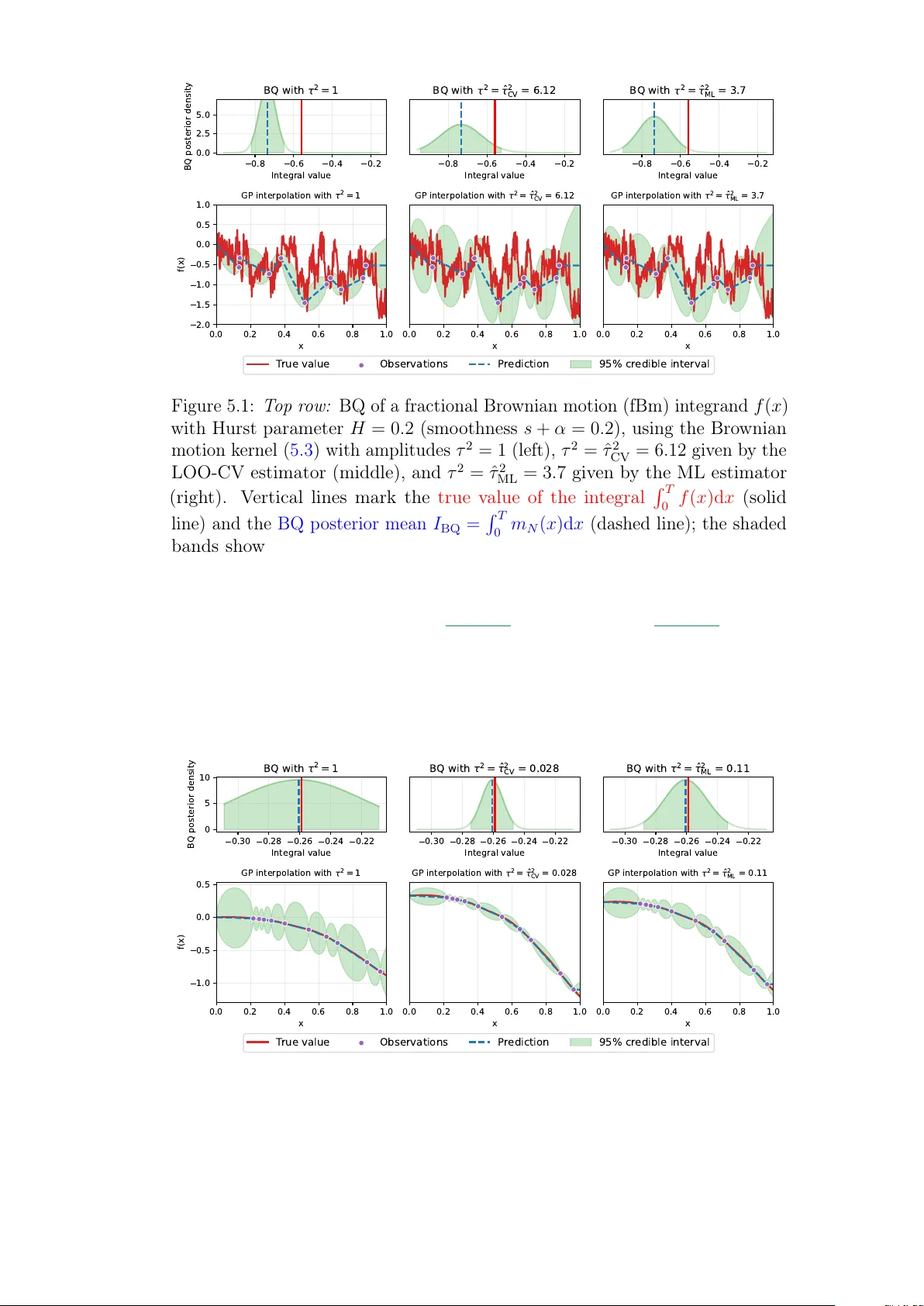
Scalable Kernel-Based Distances for Statistical Inference and In tegration Masha Naslidnyk A dissertation submitted in partial fulﬁllmen t of the requiremen ts for the degree of Do ctor of Philosoph y of Univ ersit y College London . Departmen t of Computer Science Univ ersit y College London F ebruary 26, 2026 1 Abstract Represen ting, comparing, and measuring the distance b et w een probabilit y distributions is a k ey task in computational statistics and mac hine learning. The c hoice of represen tation and the asso ciated distance determine prop erties of the metho ds in which they are used: for example, certain distances can allo w one to enco de robustness or smo othness of the problem. Kernel metho ds oﬀer ﬂexible and ric h Hilb ert space representations of distributions that allo w the mo deller to enforce properties through the choice of kernel, and estimate asso ciated distances at eﬃcien t nonparametric rates. In particular, the maximum mean discrepancy (MMD), a k ernel-based distance constructed by comparing Hilb ert space mean functions, has received signiﬁcan t attention due to its computational tractabilit y and is fa v oured b y practitioners. In this thesis, we conduct a thorough study of k ernel-based distances with a fo cus on eﬃcien t computation, with core con tributions in Chapters 3 to 6 . P art I of the thesis is fo cused on the MMD, sp eciﬁcally on improv ed MMD estimation. In Chapter 3 we prop ose a theoretically sound, impro v ed estimator for MMD in sim ulation-based inference. Then, in Chapter 4 , we prop ose an MMD-based estimator for conditional exp ectations, a ubiquitous task in statistical computation. Closing P art I , in Chapter 5 we study the problem of calibration when MMD is applied to the task of in tegration. In Part I I , motiv ated by the recent dev elopmen ts in kernel embeddings b ey ond the mean, w e introduce a family of nov el kernel-based discrepancies: k ernel quan tile discrepancies. These address some of the pitfalls of MMD, and are sho wn through b oth theoretical results and an empirical study to oﬀer a comp etitiv e alternative to MMD and its fast approximations. W e conclude with a discussion on broader lessons and future work emerging from the thesis. 2 A c kno wledgemen ts Pursuing a PhD w as something I had long dreamed of. After sev en y ears w orking in the industry , it still felt like the right next step; when I got m y acceptance, it barely felt real. Ev erything shifted after that momen t. Ov er the next four y ears, I was luc ky to explore new ideas and join the academic comm unit y . There were ups and downs, but nothing matc hes the freedom and creativit y I found in this w ork. I feel very fortunate. First, I’m grateful to my sup ervisors: Carlo Cilib erto, for unw a v ering sup- p ort and timely insight; Jeremias Knoblauc h, for inspiring passion and radical honest y; and F rançois-Xavier Briol, m y ﬁrst sup ervisor, for y our consisten t generosit y with time, your deep in v estmen t in my dev elopmen t, and for showing, b y example, that passion in research can b e sustainable. I learned so m uc h from y ou, and hop e to ha v e the privilege of passing it on. Researc h is a collab orative adven ture. I’m grateful to A yush Bharti, Siu Lun (Alan) Chau, Zonghao (Hudson) Chen, Arthur Gretton, T oni Karv onen, Oscar Key , Maren Mahsereci, Motonobu Kanaga w a, and Krik amol Muandet for their time and exp ertise; the w ork in this thesis w ould not ha v e b een p ossible without you. Thank you to Ti John, Antonin Sc hrab, Harita Dellap orta, Di mitri Meunier, Hugh Dance, Nathaël Da Costa, T akuo Matsubara, and Xing Liu for enligh tening conv ersations. Being part of a team makes all the diﬀerence; to ev ery one in The F undamen tals of Statistical Machine Learning Group, thank y ou for four years of lively discussions, coun tless cross-reviews, and the little things that k ept the da ys ligh t. Bianca, thank y ou for the many reality chec ks and for encouraging me to go for things, whether a PhD application or a swim under a waterfall. Maren, thank you for b elieving in me when there weren’t many reasons to, and for 3 in tro ducing me to the world of GPs. Prof. Danila Proskurin, y our early guidance and encouragemen t to explore researc h c hanged m y life. T o friends and family: thank you for making life joyful. I’v e b een terriﬁed of leaving someone out for all four years, so I’ll say this instead: if we shared a laugh, an adv en ture, or a slice of cak e, thank y ou. I’m grateful for y ou. T o Sunil: thank you for sharing your life with me and making ev erything b etter. T o Puﬀ, my hairiest collab orator: woof woof, bark. Go o d b oy . T o m y parents, whose strength and lo v e are unmatched, who taught me to alw a ys make space for lightness and laughter, esp ecially when things gro w hea vy: I am lucky to b e y our daugh ter. This is all thanks to you. 4 Con ten ts 1 In tro duction 11 1.1 F rom tests to measures of discrepancy . . . . . . . . . . . . . . 12 1.2 The MMD and its applications . . . . . . . . . . . . . . . . . . . 14 1.3 MMD for in tegration: kernel and Bay esian quadrature . . . . . 15 1.4 Challenges and con tributions . . . . . . . . . . . . . . . . . . . . 16 2 Bac kground 18 2.1 Kernels and repro ducing k ernel Hilb ert spaces . . . . . . . . . . 19 2.2 MMD-minimising n umerical in tegration . . . . . . . . . . . . . . 28 2.3 Quan tifying smo othness of functions . . . . . . . . . . . . . . . 33 I No v el Metho ds Based on the MMD 42 3 Eﬃcien t MMD Estimators for Sim ulation Based Inference 43 3.1 Sim ulation-Based Inference with the MMD . . . . . . . . . . . . 45 3.2 Optimally-W eigh ted Estimators . . . . . . . . . . . . . . . . . . 49 3.3 Theoretical Guaran tees . . . . . . . . . . . . . . . . . . . . . . . 50 3.4 Exp erimen ts . . . . . . . . . . . . . . . . . . . . . . . . . . . . . 53 3.5 Conclusion . . . . . . . . . . . . . . . . . . . . . . . . . . . . . . 59 4 MMD-based Estimators for Conditional Exp ectations 61 4.1 Computing Conditional Exp ectations . . . . . . . . . . . . . . . 63 5 4.2 Conditional Ba y esian Quadrature . . . . . . . . . . . . . . . . . 65 4.3 Theoretical Guaran tees . . . . . . . . . . . . . . . . . . . . . . . 67 4.4 Exp erimen ts . . . . . . . . . . . . . . . . . . . . . . . . . . . . . 70 4.5 Conclusions . . . . . . . . . . . . . . . . . . . . . . . . . . . . . 76 5 Calibration for MMD-minimising In tegration 77 5.1 Uncertain t y Quan tiﬁcation via Kernel Scaling . . . . . . . . . . 78 5.2 Kernel parameter estimation . . . . . . . . . . . . . . . . . . . . 85 5.3 Setting . . . . . . . . . . . . . . . . . . . . . . . . . . . . . . . . 88 5.4 Theoretical Analysis . . . . . . . . . . . . . . . . . . . . . . . . 92 5.5 Consequences for credible in terv als . . . . . . . . . . . . . . . . 99 5.6 Exp erimen ts . . . . . . . . . . . . . . . . . . . . . . . . . . . . . 103 5.7 Conclusion . . . . . . . . . . . . . . . . . . . . . . . . . . . . . . 106 I I Kernel-Based Distances Bey ond the MMD 109 6 Kernel Quan tile Em beddings 110 6.1 Preliminaries: Quantiles and W asserstein distances . . . . . . . 112 6.2 Kernel Quan tile Em b eddings and Discrepancies . . . . . . . . . 115 6.3 Gaussian Kernel Quan tile Discrepancy . . . . . . . . . . . . . . 122 6.4 Exp erimen ts . . . . . . . . . . . . . . . . . . . . . . . . . . . . . 123 6.5 Conclusion . . . . . . . . . . . . . . . . . . . . . . . . . . . . . . 129 I I I Discussion and F uture W ork 131 Bibliograph y 135 A Eﬃcien t MMD Estimators for Sim ulation Based Inference: Supplemen tary Materials 169 A.1 Pro ofs of Theoretical Results . . . . . . . . . . . . . . . . . . . . 169 6 A.2 Exp erimen tal details . . . . . . . . . . . . . . . . . . . . . . . . 183 B MMD-based Estimators for Conditional Exp ectations: Supple- men tary Materials 186 B.1 Pro ofs of Theoretical Results . . . . . . . . . . . . . . . . . . . . 186 B.2 Hyp erparameter Selection . . . . . . . . . . . . . . . . . . . . . 206 B.3 Exp erimen tal details . . . . . . . . . . . . . . . . . . . . . . . . 209 B.5 Reducing the cost of Ba y esian Quadrature . . . . . . . . . . . . 219 C Calibration for MMD-minimising In tegration: Supplemen tary Materials 220 C.1 Proofs of Theoretical Results . . . . . . . . . . . . . . . . . . . . 220 C.2 F urther discussion on Theorem 17 . . . . . . . . . . . . . . . . 240 C.3 Explicit expression for the leav e- p -out estimator . . . . . . . . . 240 C.4 Comparison of CV and ML estimators for Matérn kernels . . . . 241 D Kernel Quan tile Em b eddings: Supplementary Materials 244 D.1 Probability Metrics and Their Estimators . . . . . . . . . . . . 244 D.2 Connection b etw een Centered and Uncentered Quantiles . . . . 251 D.3 Pro ofs of Theoretical Results . . . . . . . . . . . . . . . . . . . . 254 D.4 Additional Numerical Results . . . . . . . . . . . . . . . . . . . 271 7 List of Figures 3.1 Illustration of an optimally-w eigh ted MMD estimator for SBI. . 44 3.2 Error in estimating MMD 2 for the m ultiv ariate g-and-k distribution. 56 3.3 ABC p osteriors for the wind farm mo del. . . . . . . . . . . . . . 59 4.1 Illustration of c onditional Bayesian quadr atur e (CBQ). . . . . . 63 4.2 Ba y esian sensitivit y analysis for linear mo dels. . . . . . . . . . . 70 4.3 Ba y esian linear mo del sensitivity analysis in d = 2 . . . . . . . . 71 4.4 Ba y esian sensitivit y analysis for SIR Mo del & Option pricing in mathematical ﬁnance. . . . . . . . . . . . . . . . . . . . . . . . 73 4.5 Uncertain t y decision making in health economics. . . . . . . . . 75 5.1 BQ of a fractional Bro wnian motion in tegrand. . . . . . . . . . . 80 5.2 BQ of an in tegrated fractional Bro wnian motion in tegrand. . . . 80 5.3 Illustrating rates in Theorems 14, 15 and 20. . . . . . . . . . . . 94 5.4 Illustrating rates in Theorems 18, 19 and 21. . . . . . . . . . . . 97 5.5 Asymptotics of CV estimators for functions of v arying smo othness. 107 5.6 Asymptotics of CV estimator compared to asymptotics of ML estimators. . . . . . . . . . . . . . . . . . . . . . . . . . . . . . . 108 6.1 Illustration of biv ariate quantiles. . . . . . . . . . . . . . . . . . 113 6.2 Illustration of the impact of the slicing direction on K QEs. . . . 118 6.3 Exp erimen tal results comparing K QDs with baseline approac hes. 124 6.4 Run time comparison of K QDs against baseline metho ds. . . . . 129 8 C.1 Rates of deca y for the ML and CV estimators for the Matérn k ernel . . . . . . . . . . . . . . . . . . . . . . . . . . . . . . . . 242 C.2 Asymptotics of CV estimator compared to asymptotics of the ML estimator, for the Matérn k ernel . . . . . . . . . . . . . . . 243 D.1 Type I control on CIF AR-10 vs. CIF AR-10.1. . . . . . . . . . . 271 D.2 Exp erimen tal results comparing KQDs with baseline approaches, for p = 1 . . . . . . . . . . . . . . . . . . . . . . . . . . . . . . . 272 D.3 Gaussian KQD test p ow er under diﬀerent weigh ting measures. . 274 D.4 KQD vs. MMD based on other KME approximations . . . . . . 275 9 List of T ables 2.1 Summary of notation used in the thesis. . . . . . . . . . . . . . 20 2.2 Example k ernels. . . . . . . . . . . . . . . . . . . . . . . . . . . 23 3.1 Benc hmarking O W-MMD on p opular sim ulators. . . . . . . . . 54 3.2 Comp osite go odness-of-ﬁt test with V-statistic vs. OW-MMD. . 58 A.1 Computational and sample complexity of the V-statistic vs. O W-MMD. . . . . . . . . . . . . . . . . . . . . . . . . . . . . . 183 A.2 Hyp erparameters in the comp osite go odness-of-ﬁt test. . . . . . 184 B.1 V ariables in the health economics exp erimen t. . . . . . . . . . . 217 10 Chapter 1 In tro duction The distinction b et w een a ‘test’ and a ‘measure’ of group diverge nce is fundamental: a test merely tells us whether the tw o groups (from whic h the tw o given samples are drawn) are diﬀerent or not, while a measure giv es us a quan titativ e estimate of the magnitude of the diﬀerence (if any) b etw een the t w o groups. Mahalanobis [ 1930 ] Comparing t w o probabilit y distributions P , Q is a k eystone of man y metho ds in computational statistics and mac hine learning. A t their core, a wide range of fundamental tasks can b e framed as questions ab out whic h distributions are closer or farther apart under some notion of discrepancy D ( P , Q ) : • Hyp othesis testing [ Salicrú et al. , 1994 , Sejdinovic et al. , 2012 ]: do es the observ ed discrepancy b etw een P and Q exceed what is exp ected under the n ull h yp othesis of zero discrepancy? This includes tw o-sample (empiri cal vs. empirical), go o dness-of-ﬁt (empirical vs. mo del), and indep endence (join t vs. pro duct of marginals) testing. • P arameter estimation and inference [ Basu et al. , 2011 , Briol et al. , 2019a ]: whic h p oin t estimate or p osterior distribution o v er a parameter θ places w eigh t on mo dels P θ that are close to the observ ed data distribution Q under D ? • Numerical in tegration [ Da vis and Rabinowitz , 2007 , Karvonen and Särkkä , 2017 ]: which choice of p oints and weigh ts { x n , w n } N n =1 in R X f ( x ) P ( d x ) ≈ 11 P N n =1 w n f ( x n ) minimises the discrepancy b et w een the w eigh ted empirical distribution P N n =1 w n δ x n and the in tegration measure P ? • Domain adaptation and generativ e modelling [ Gretton et al. , 2009b , A cuna et al. , 2021 ]: what transformation T on th e input space of the source distribution P minimises the discrepancy b et w een the transformed T # P and the target Q ? • Dataset summarisation and thinning [ Dwiv edi and Mack ey , 2024 , Mak and Joseph , 2018 ]: whic h subset of samples { y m } M m =1 ⊆ { x n } N n =1 minimises the discrepancy b etw een the empirical distributions 1 / M P M m =1 δ y m and 1 / N P N n =1 δ x n ? In eac h of these examples, the c hoice of discrepancy determines the prop- erties of the metho d addressing the task. This raises a central question: what mak es a ‘go o d’ discrepancy? At the v ery least, the discrepancy should b e able to tell diﬀerent distributions apart: P  = Q should imply D ( P , Q ) > 0 . It should also b e computationally conv enient, with eﬃcien t estimators that do not suﬀer from the ‘curse of dimensionality’. Ideally , to enable optimisation, the gradien ts of the discrepancy should b e eﬃcien tly computable as w ell. The maximum me an discr ep ancy (MMD, Borgw ardt et al. [ 2006 ], Gretton et al. [ 2012a ]), a k ernel-based notion of discrepancy that compares means of certain distributional em b eddings, satisﬁes these desiderata, leading to its widespread adoption. Ho w ev er, its practical application reveals k ey c hallenges: standard estimators can b e ineﬃcien t, and the reliance on mean embeddings can b e restrictiv e. This thesis addresses these limitations by developing kernel-based discrepancies and estimators that are more eﬃcien t, expressiv e, and robust. T o situate these contributions, w e b egin with the historical context from whic h these metho ds emerged, b efore turning to the MMD and then outlining the c hallenges that motiv ate the thesis. 1.1 F rom tests to measures of discrepancy The idea of discrepancy b etw een probability distributions as a cen tral ob ject of study in statistical metho dology is not new. In the early 20th cen tury , classiﬁcation problems in biology and anthropology motiv ated statisticians 12 to dra w a sharp line b etw een tests of gr oup diver genc e (in to day’s terms, h yp othesis tests giving a reject/do not reject answer) and me asur es of gr oup diver genc e (discrepancies b et w een empirical distributions), and explicitly argue for general-purp ose, non-ad ho c discrepancies as a metho dological foundation. Mahalanobis [ 1936 ] established this line of work with the introduction of what is no w called the Mahalanobis distance, which measures how far a p oin t lies from a distribution while accoun ting for correlations b et w een v ariables; Bhattac haryy a [ 1943 ] generalised this idea to deﬁne a discrepancy b et w een t w o distributions. Since then, man y further notions of discrepancies and discrepancy-based metho ds in statistical and machine learning hav e b een prop osed: some nov el, others extending existing statistics in to discrepancy measures. F or ex am- ple, Csiszár [ 1963 ] reinterpreted the statistic in Pearson’s χ 2 test as a dis- crepancy: sp eciﬁcally , a χ 2 -div ergence, a kind of f -div ergence. f -div ergences quan tify the discrepancy b etw een distributions through their ratios: for a con v ex function f , the f -div ergence b et w een P and Q is deﬁned as D f ( P , Q ) = E X ∼ Q [ f ◦ d P / d Q ]( X ) , the exp ected v alue under Q of f comp osed with the Radon-Nikodym deriv ative of P with resp ect to Q . Important discrepancies, such as the total v aria- tion distance [ v an der V aart , 1998 , Section 2.9], the Kullbac k–Leibler diver- gence [ Kullbac k and Leibler , 1951 ], and the aforemen tioned χ 2 -div ergence are all f -div ergences for diﬀeren t c hoices of f . The main b eneﬁt of the f -div ergences is the interpretabilit y of the ratio d P / d Q ; ho w ev er, it is only well-deﬁned when P is absolutely contin uous with resp ect to Q , whic h in turn requires the supp ort of P to lie within the supp ort of Q . Additionally , estimating f -div ergences is a notoriously c hallenging task: the f -div ergence b et w een empirical distributions, D f ( P N , Q N ) , do es not conv erge to the f -div ergence b et w een true distributions D f ( P , Q ) , as N → ∞ [ P eyré and Cuturi , 2019 , Section 8.4.2]. The prop osed alternativ e nonparametric and neural netw ork-based estimators suﬀer from the curse of dimensionality , conv erging at rates as slo w as N − 1 /d unless f and d P / d Q exhibit suﬃcien t smo othness [ Rub enstein et al. , 2019 , McAllester and Stratos , 2020 , Nguy en et al. , 2010 ]. 13 Another ma jor family of discrepancies is motiv ated by a classic result on uniqueness of the represen tation of probability measures via integrals of b ounded con tin uous functions [ Dudley , 2002 , Lemma 9.3.2]: any tw o distributions P , Q on a metric space ( X , d ) coincide if and only if E X ∼ P f ( X ) = E Y ∼ Q f ( Y ) for all con tin uous and b ounded functions f : X → R . This class of functions, while expressiv e, is prohibitiv ely large for practical applications. Inte gr al pr ob abilit y pseudometrics (IPMs, Müller [ 1997 ]) are a generalisation of this idea to an arbitrary class of real-v alued functions F , deﬁned as IPM F ( P , Q ) = sup f ∈F | E X ∼ P f ( X ) − E Y ∼ Q f ( Y ) | . (1.1) T rivially , when F con tains all con tin uous functions b ounded by some constan t, the corresp onding IPM is a metric; when F is the class of all p olynomials of order up to p , the IPM reduces to p -momen t matc hing. Other choices of F reco v er well-kno wn discrepancies, including total v ariation distance (that metrises strong con v ergence) 1 , the 1-W asserstein distance [ Kantoro vic h , 1942 , Villani , 2009 ], and the canonical kernel-based distance, the MMD. Whenev er the IPM metrises weak conv ergence, as is the case for the 1-W asserstein distance and the MMD for a large class of k ernels [ Simon-Gabriel et al. , 2023 ], the IPM b et w een empirical distributions is a consistent estimator of the true IPM. Its sample complexity dep ends on the class F ; for example, the 1-W asserstein distance estimator con v erges at the slow rate of N − 1 /d , unless the distributions are supp orted on a lo w er-dimensional manifold [ F ournier and Guillin , 2015 ]. 1.2 The MMD and its applications When F = B H k , the unit ball of some r epr o ducing kernel Hilb ert sp ac e (RKHS, Berlinet and Thomas-Agnan [ 2004 ]) H k with inner pro duct ⟨· , ·⟩ H k induced b y a r epr o ducing kernel k : X × X → R , the corresp onding IPM, the MMD, is particularly computationally attractive. Unlike other common IPMs, the MMD [ Borgw ardt et al. , 2006 , Gretton et al. , 2012a ] is av ailable in closed functional form: owing to the rich structure of the RKHS, the MMD b etw een P and Q is exactly the RKHS inner pro duct norm of µ k, P − µ k, Q , the diﬀerence 1 Curiously , total v ariation distance is, up to a constant scaling factor, the only discrepancy that is b oth an f -div ergence and an IPM [ Srip erum budur et al. , 2012 ]. 14 b et w een kernel me an emb e ddings [ Smola et al. , 2007 ] of P and Q , MMD k ( P , Q ) = ∥ µ k, P − µ k, Q ∥ H k . µ k, P represen ts a distribution P as a mean function in the RKHS; when the mapping P 7→ µ k, P is injectiv e, meaning the represen tation of a distribution as a k ernel mean em b edding is unique and captures all information ab out the distribution, the kernel is said to b e ‘c haracteristic’ [ Srip erum budur et al. , 2010 ]. MMD has received signiﬁcan t atten tion due to its computational tractabil- it y: its most common estimator has cost O ( N 2 ) and conv erges at the rate O ( N − 1 / 2 ) as the n um b er of datap oin ts N increases, with c heap er alternativ es prop osed [ Gretton et al. , 2012a , Chwialk o wski et al. , 2015 , Bodenham and Ka w ahara , 2023 , Schrab et al. , 2022 ]. F or this reason, the MMD has b een used to address a broad range of tasks from hypothesis testing [ Gretton et al. , 2012a ] to parameter estimation [ Briol et al. , 2019a , Chérief-Ab dellatif and Alquier , 2020 ], causal inference [ Muandet et al. , 2021 , Sejdinovic , 2024 ], feature attribution [ Chau et al. , 2022 , 2023 ], and learning on distributions [ Muandet et al. , 2012 , Szab ó et al. , 2016 ]. A particularly elegan t application, and one cen tral to this thesis, is n umerical in tegration, whic h w e cov er next. 1.3 MMD for in tegration: k ernel and Ba y esian quadrature MMD-minimising in tegration metho ds are known as kernel quadr atur e [ Som- mariv a and Vianello , 2006 , Dic k et al. , 2013 , Bach , 2017 , Kanagaw a et al. , 2020 ] or, in their probabilistic form, Bayesian quadr atur e [ Diaconis , 1988 , O’Hagan , 1991 , Hennig et al. , 2022 ]. These approac hes hav e b een used primarily in statistical computation (see Briol et al. [ 2019a ] and references therein), as w ell as in div erse scientiﬁc and engineering domains such as astronomy [ Lin et al. , 2025 ], battery design [ Kuhn et al. , 2023 ], w eather mo delling [ Osb orne et al. , 2012 ], reliabilit y engineering [ Cousin et al. , 2024 ], computer graphics [ Marques et al. , 2013 , Xi et al. , 2018 ], cardiac mo delling [ Oates et al. , 2017 ] and tsunami mo delling [ Li et al. , 2022 ]. Kernel quadrature replaces classical numerical inte- gration rules (suc h as Mon te Carlo and trap ezoidal) with weigh ted schemes in 15 whic h the weigh ts are selected to minimise the MMD, whic h can also b e shown to b e the ro ot mean squared in tegration error o v er functions sampled from a Gaussian pro cess [ Ritter , 2000 , Corollary 7 in p.40]. This view naturally leads to Ba y esian quadrature, a probabilistic in terpretation in whic h the integrand is mo delled as a Gaussian pro cess. This approach pro duces not only an estimate of the integral, but also a principled p osterior uncertain t y quantiﬁcation, and a w a y to estimate hyperparameters via empirical Bay es. These adv an tages make Ba y esian quadrature particularly app ealing when (1) function ev aluations are exp ensiv e or scarce, since accurate estimates can b e achiev ed with relatively few samples; (2) there is prior information a v ailable ab out the in tegrand that can b e incorp orated into the Gaussian pro cess; and (3) uncertaint y quantiﬁcation is imp ortan t for reliabilit y of the estimate. 1.4 Challenges and con tributions While the MMD is a widely used to ol for comparing probabilit y distributions, applying it eﬀectively in practice can b e surprisingly subtle. Its p erformance dep ends on b oth the structure of the problem and the choice of kernel, and naïv e application ma y lead to ineﬃciencies or failures in capturing imp ortant distributional features. W e now highlight tw o key practical challenges. Challenge 1: Sp ecialising MMD-based metho ds. In structured settings, suc h as simulation-based inference and conditional or m ulti-task in tegration, generic, task-agnostic uses of MMD are often outp erformed by estimators that mak e use of problem structure. F or example, for smo oth simulators, kernel mean em b edding in tegrals can b e estimated more eﬃciently than with the V-statistic; similarly , metho ds mo delling dep endencies across integrands outp erform MMD- minimising quadrature on eac h integral in isolation [ Niu et al. , 2023 , Gessner et al. , 2020 ]. These observ ations motiv ate tailored, structure-aw are MMD estimators that are more data-eﬃcien t in suc h settings. Challenge 2: Alternative kernel-based distances. When the k ernel k is not characteristic, so that MMD k ( P , Q ) = 0 do es not imply P = Q , the k ernel mean embedding fails to uniquely determine the distribution, limiting the reliabilit y of MMD for distribution comparison. F urther, even when k is c haracteristic, alternativ e kernel-based discrepancies that prob e information 16 b ey ond the k ernel mean may capture distributional diﬀerences more eﬃciently in the ﬁnite-sample regime. These c hallenges motiv ate the core contributions of the thesis. Chapter 2 pro vides the necessary technical background and to ols, in troducing kernel metho ds, MMD-based numerical integration, and function smo othness. The remaining c hapters address the t w o c hallenges in turn. • In P art I , we fo cus on the ﬁrst challenge: improving MMD estimators in structured settings. In Chapter 3 , we prop ose an optimal ly-weighte d estimator of the MMD in sim ulation-based inference, by making use of Bay esian quadrature, an MMD-minimising integration metho d, to impro v e estimation of k ernel means. Then, in Chapter 4 , we prop ose conditional Bay esian quadrature, an MMD-based estimator extending Ba y esian quadrature to computing conditional exp ectations, a task that arises frequently in statistical computation. Lastly , in Chapter 5 , we turn to the issue of calibration in Bay esian quadrature, sp eciﬁcally amplitude h yp erparameter selection and its impact on uncertain t y quantiﬁcation. • In P art I I , w e mov e b eyond the MMD and consider alternative general- purp ose k ernel-based discrepancies. Motiv ated by recen t adv ances in k ernel em b eddings b ey ond the mean, we in tro duce a new family of k ernel-based statistical distances, the k ernel quan tile discrepancies. These discrepancies mitigate some of the shortcomings of MMD, and w e sho w through b oth theoretical analysis and empirical study that they oﬀer a comp etitiv e alternativ e to MMD and its fast appro ximations. 17 Chapter 2 Bac kground In the previous chapter, we brieﬂy survey ed discrepancies b etw een probability distributions and outlined challenges addressed in this thesis. This chapter in tro duces k ey concepts and to ols needed for our results, and sets the nota- tion used in later c hapters. First, ho w ev er, a clarifying note on fundamen tal terminology . Discrepancy vs. div ergence vs. distance. Let P b e some space of prob- abilit y distributions, and let P , Q , P ′ b e some distributions in P . In mo dern statistics and mac hine learning, a discr ep ancy is any non-negativ e function D : P × P → [0 , ∞ ] in tended to quan tify distributional dissimilarit y; it is t ypically required that D ( P , P ) = 0 . A diver genc e is a discrepancy that also satisﬁes the identity of indisc ernibles , i.e., D ( P , Q ) = 0 if and only if P = Q . A distanc e is the strongest notion of dissimilarity: it is a divergence that is ﬁnite, symmetric, D ( P , Q ) = D ( Q , P ) , and satisﬁes the triangle inequality , D ( P , Q ) ≤ D ( P , P ′ ) + D ( P ′ , Q ) , so that D is a metric on P . T erminology in the literature is not alwa ys consistent, owing to historical usage or notational sim- pliﬁcations. F or example, the Bhattacharyy a distance is, strictly sp eaking, only a diverge nce, and integral probabilit y pseudometrics (IPMs) are con v en tionally called ‘metrics’ despite b eing merely pseudometrics unless the function class is ric h enough to guarantee the iden tit y of indiscernibles. Moreov er, whether a giv en discrepancy is a distance or a div ergence ma y dep end on the c hoice of domain P : for instance, the p -W asserstein distance W p for p ≥ 1 is a distance only on the space of probabilit y distributions with ﬁnite p -th momen t. In what follo ws, w e will tak e care to k eep these distinctions explicit. 18 In the rest of the c hapter, we introduce core concepts in kernel and repro ducing k ernel Hilb ert space theory , as w ell as more sp eciﬁc details necessary to in troduce the setting of our results. Throughout the work, X denotes the input space or set; in the most general setting, X is a set, and in the most sp eciﬁc setting, X is a subset of R d . W e clarify the restrictions on X throughout. W e aim to deﬁne all notation b efore using it, and give frequent explanations of its meaning in text. Ho w ev er, to aid readability , we giv e a short summary of notation used in this w ork in T able 2.1 . 2.1 Kernels and repro ducing k ernel Hilb ert spaces Recall that a symmetric N × N matrix k ( x 1: N , x 1: N ) is said to b e p ositive deﬁnite if for an y v ector α 1: N ∈ R N , it holds that α ⊤ 1: N k ( x 1: N , x 1: N ) α 1: N ≥ 0 . Deﬁnition 1 (Positiv e deﬁnite kernel) . A symmetric function k : X × X → R on a set X is a p ositive deﬁnite kernel if the Gram matrix [ Berlinet and Thomas-Agnan , 2004 , Section 2] k ( x 1: N , x 1: N ) : =      k ( x 1 , x 1 ) . . . k ( x 1 , x N ) . . . . . . . . . k ( x N , x 1 ) . . . k ( x N , x N )      is p ositiv e deﬁnite, for an y N ∈ N ≥ 1 and an y x 1: N ∈ X N . W e will simply refer to p ositiv e deﬁnite k ernels as ‘kernels’. When α ⊤ 1: N k ( x 1: N , x 1: N ) α 1: N = 0 for m utually distinct x 1: N ∈ X N implies α 1 = · · · = α N = 0 , the k ernel is said to b e strictly p ositive deﬁnite . Commonly used kernels, suc h as the Gaussian kernel and the Matérn family of k ernels in tro duced b elo w, are strictly p ositive deﬁnite. Remark 1. The terminology in the literature can b e inconsistent, with kernels as deﬁned in Deﬁnition 1 referred to as p ositiv e semi deﬁnite, and reserving the term p ositiv e deﬁnite for k ernels that w e call strictly p ositive deﬁnite. The concepts and results in tro duced in this chapter, and the rest of the 19 N The set of natural num bers, { 0 , 1 , . . . } . N ≥ a The subset { a, a + 1 , . . . } ⊆ N , for a ∈ N . Id d The d × d identit y matrix. x 1: N ∈ X N T uple ( x 1 , x 2 , . . . , x N ) , for x 1 , . . . , x N ∈ X . x 1: N ∈ R N × d V ector (for d = 1 ) or matrix h x 1 x 2 . . . x N i ⊤ , for x 1 , . . . , x N ∈ X ⊆ R d . ∥ · ∥ F , ⟨· , ·⟩ F The norm and inner pro duct of a space F . f ( x 1: N ) ∈ R N Column v ector h f ( x 1 ) f ( x 2 ) . . . f ( x N ) i ⊤ , for x 1 , . . . , x N ∈ X and f : X → R . k ( x 1: N , x 1: N ) ∈ R N × N Gram matrix     k ( x 1 , x 1 ) . . . k ( x 1 , x N ) . . . . . . . . . k ( x N , x 1 ) . . . k ( x N , x N )     , for x 1 , . . . , x N ∈ X and k : X × X → R . ∥ · ∥ 2 Euclidean norm. F or a ∈ R d , ∥ a ∥ 2 = q P d i =1 a 2 i . H k RKHS induced b y a k ernel k (see Deﬁnition 4 ). µ k, P ∈ H k Kernel mean em b edding of P in H k (see Deﬁni- tion 5 ). C s ( X ) Space of s -times con tin uously diﬀeren tiable func- tions on X (see Deﬁnition 8 ). C s,α ( X ) Hölder space (see Deﬁnition 10 ). L p ( X , P ) L p space, for a measure P on X (see Deﬁni- tion 11 ). L p ( X ) L p space, for the Leb esgue measure µ on X (see Deﬁnition 11 ). W s,p ( X ) Sob olev space (see Deﬁnition 13 ). X , X ′ ∼ N ( µ, Σ) X , X ′ are indep enden t random v ariables; the law of eac h is the Gaussian distribution with mean µ and co v ariance Σ . X ∼ ν X is a random v ariable the law of whic h is the measure ν . P N = 1 N P N n =1 δ x n An equally-w eigh ted empirical measure, x 1 , . . . , x N ∼ P . P w N = P N n =1 w n δ x n A w eigh ted empirical measure, x 1 , . . . , x N ∼ P . T able 2.1: Summary of notation used in the thesis. thesis, hold for k ernels as deﬁned in Deﬁnition 1 ; whenev er a distinction with strictly p ositiv e deﬁnite k ernels is helpful, w e will mak e it clear. 20 2.1.1 Examples and basic prop erties of k ernels The k ernel c hoice is central in kernel-based discrepancies. First, the kernel determines general task-agnostic prop erties: whether the discrepancy is a distance [ Srip erum budur et al. , 2011 ], the topology it induces on probabilit y distributions [ Simon-Gabriel et al. , 2023 , Barp et al. , 2024 ], and what dif- ferences b et w een the distributions it emphasises [ Rahimi and Rec h t , 2007 , Srip erum budur and Szab ó , 2015 ]. Second, the kernel may driv e task-sp eciﬁc p erformance: as discussed in Section 2.2 , MMD-minimising in tegration can b e view ed as Gaussian pro cess regression with k ernel k on the in tegrand f ; adapting k to matc h prop erties of f accelerates con v ergence and improv es uncertain t y calibration [ Kanaga w a et al. , 2020 , W ynne et al. , 2021 ]. T able 2.2 lists commonly used k ernels that are inv oked in this thesis. The amplitude p ar ameter τ 2 > 0 scales the outpu t of the kernel, and is instrumental in uncertaint y quan tiﬁcation; this is discussed further in Chapter 5 . The lengthscale parameter l > 0 in the Matérn and Gaussian kernels scales the input, as the distance ∥ x − x ′ ∥ 2 gets scaled b y l . Matérn k ernels are of particular interest: the or der parameter ν determines the smo othness of k ν ; this will b e formalised further in Section 2.3.3 . F urther, for half-in teger orders ν ∈ { 1 / 2 , 3 / 2 , . . . } , the k ernel k ν tak es a con v enien t form: it is a pro duct of an exp onen tial and a p olynomial of degree ⌊ ν ⌋ [ Rasm ussen and Williams , 2006 ]. F or example, for the ﬁrst three half-integers, and ρ = ∥ x − x ′ ∥ 2 , ν = 1 / 2 : k ν ( x, x ′ ) = τ 2 exp  − ρ l  ν = 3 / 2 : k ν ( x, x ′ ) = τ 2 1 + √ 3 ρ l ! exp − √ 3 ρ l ! ν = 5 / 2 : k ν ( x, x ′ ) = τ 2 1 + √ 5 ρ l + 5 ρ 2 3 l 2 ! exp − √ 5 ρ l ! A t the limit ν → ∞ , k ν go es to the inﬁnitely smo oth Gaussian k ernel k Gauss . P olynomial kernels illustrate t w o phenomena. First, a p olynomial k ernel is not strictly p ositiv e deﬁnite: ev en more strongly , a Gram matrix for any pairwise distinct x 1: N for a large enough N is not strictly p ositiv e deﬁnite [ Rasmussen 21 and Williams , 2006 , Section 4.2.2]. Second, the MMD with the p olynomial k ernel is not a distance on the space of Borel probability measures; this example is instrumen tal in pro ofs in Chapter 6 . The Bro wnian motion k ernel is w ell-studied [ Mörters and Peres , 2010 ] and is in tegral to man y ﬁelds of study , from calculus on general sto c hastic pro cesses to mo delling ph ysics and biological phenomena. The fractional Bro wnian motion k ernel k 0 ,H [ Mandelbrot , 1982 , Chapter IX], with its smo othness parameterised b y the Hurst parameter H , generalises the Bro wnian motion k ernel: for H > 1 / 2 , the fractional Bro wnian motion k ernel is smo other than the regular Bro wnian motion k ernel; for H < 1 / 2 it is less smo oth. It is easy to see that k 0 , 1 / 2 is the Bro wnian motion kernel k BM . W e mak e ‘smoothness’ precise and discuss the prop erties of the (fractional) Bro wnian motion k ernel in Section 5.3.3 . All kernels in T able 2.2 , except for the p olynomial ones, are strictly p ositiv e deﬁnite; this prop ert y is cen tral to MMD-minimising in tegration in Chapter 4 . The Matérn and Gaussian kernels additionally satisfy t w o imp ortan t prop erties, b oundedness and stationarit y , whic h w e now deﬁne and discuss. Deﬁnition 2. A kernel k is said to b e b ounded if there exists a constant B > 0 suc h that k ( x, x ) ≤ B for an y x ∈ X . In fact, this is equiv alen t to | k ( x, x ′ ) | ≤ B for all pairs x, x ′ ∈ X : b y k b eing p ositiv e deﬁnite, it holds that k ( x, x ) − 2 k ( x, x ′ ) + k ( x ′ , x ′ ) ≥ 0 and k ( x, x ) + 2 k ( x, x ′ ) + k ( x ′ , x ′ ) ≥ 0 , with equality when x = x ′ ; therefore | k ( x, x ′ ) | ≤ ( k ( x, x ) + k ( x ′ , x ′ )) / 2 ≤ B . Deﬁnition 3. A k ernel k is said to b e stationary , translation-inv ariant, or shift-in v arian t, if it only dep ends on the diﬀerence x − x ′ , i.e., there is a function k 0 suc h that k ( x, x ′ ) = k 0 ( x − x ′ ) . A stationary k ernel k is automatically b ounded b y B = k 0 (0) ; for Matérn and Gaussian kernels, k 0 (0) = τ 2 . Both are imp ortan t prop erties in the context of MMD. Boundedness (and measurability) of k is suﬃcien t for MMD k ( P , Q ) to b e well deﬁned and ﬁnite for all Borel probability measures P , Q . F urther, if k is contin uous and stationary on X = R d , then MMD k is a distanc e on 22 P olynomial of degree q k Poly ( x, x ′ ) = τ 2 ( x ⊤ x ′ + c ) q , for c ≥ 0 and q ∈ N . Matérn of order ν , and smo othness s = ν + d/ 2 k ν ( x, x ′ ) = τ 2 Γ( ν )2 ν − 1 ( √ 2 ν l ∥ x − x ′ ∥ 2 ) ν K ν ( √ 2 ν l ∥ x − x ′ ∥ 2 ) , where K ν for ν > 0 is the mo diﬁed Bessel function of the second kind. Gaussian k Gauss ( x, x ′ ) = τ 2 exp( −∥ x − x ′ ∥ 2 2 / (2 l 2 )) Bro wnian motion k BM ( x, x ′ ) = τ 2 min( x, x ′ ) F ractional Bro wnian motion k 0 ,H ( x, x ′ ) = τ 2  x 2 H + x ′ 2 H − | x − x ′ | 2 H  / 2 T able 2.2: Example kernels on X = R d . F or Bro wnian motion and fractional Bro wnian motion, X = [0 , ∞ ) . the set of Borel probabilit y measures if and only if the supp ort of the F ourier transform of k 0 is the entire R d ; this condition holds for b oth Matérn and Gaussian k ernels [ Srip erum budur et al. , 2010 ]. W e return to these p oints, and their role in our results, in Section 2.1.3 . 2.1.2 Repro ducing kernel Hilb ert spaces Ev ery positive deﬁnite kernel k : X × X → R deﬁnes a unique repro ducing k ernel Hilb ert space H k of functions X → R . This one-to-one mapping is p o w erful: it lets us work with rich, often inﬁnite-dimensional, function spaces by manipulating only the k ernel; for example, prop erties of k , suc h as smo othness, b oundedness, and p erio dicit y , are inherited by functions in the RKHS. Before giving the formal deﬁnition of an RKHS, w e brieﬂy review the construction of H k from k ; this construction illuminates the deﬁnition and underlies the pro of that the map k 7→ H k is one-to-one. F or an in-depth treatmen t of RKHS theory , w e refer the reader to Berlinet and Thomas-Agnan [ 2004 ]. Remark 2 (Equiv alen t deﬁnitions of an RKHS) . There are m ultiple equiv alent deﬁnitions of an RKHS: (1) as a Hilb ert space with contin uous ev aluation functionals; (2) as a closure of the span of k ( x, · ) ; (3) as a Hilb ert space with a repro ducing k ernel. W e use (3) as the primary deﬁnition, review (2), and presen t the equiv alence b et w een (2) and (3) as a theorem [ Berlinet and Thomas- Agnan , 2004 , Mo ore–Aronsza jn theorem]. Lastly , though w e do not review it, the equiv alence b et w een (1) and (3) is a corollary of the Riesz representation theorem [ Berlinet and Thomas-Agnan , 2004 , Theorem 1]. Consider a space H 0 k = span { k ( x, · ) | x ∈ X } consisting of all func- tions f : X → R of the form f ( x ) = P N n =1 a n k ( x n , x ) for an y N ∈ N ≥ 1 23 and a 1: N ∈ R N , x 1: N ∈ X N . Deﬁne a function ⟨· , ·⟩ H 0 k : H 0 k × H 0 k → R as ⟨ f , g ⟩ H 0 k = P N n =1 P M m =1 a n b m k ( x n , y m ) for an y f = P N n =1 a n k ( x n , · ) and g = P M m =1 b m k ( y m , · ) . It is easy to sho w ⟨· , ·⟩ H 0 k is an inner pro duct on H 0 k , and for an y f ∈ H 0 k and x ∈ X it holds that ⟨ f , k ( x, · ) ⟩ H 0 k = f ( x ) . (2.1) Under the metric induced by ⟨· , ·⟩ H 0 k , the space H 0 k need not b e complete, meaning there ma y b e a Cauch y sequence { f n } n ∈ N that do es not ha v e a limit in H 0 k . W e deﬁne H k , the r epr o ducing kernel Hilb ert sp ac e induced by k , as the completion of H 0 k . F or every f ∈ H k , there will b e a Cauch y sequence { f n } n ∈ N ∈ H 0 k that p oin t wise conv erges to f ; this allo ws us to deﬁne ⟨ f , g ⟩ H k = lim n →∞ ⟨ f n , g n ⟩ H 0 k , (2.2) whic h can b e sho wn to b e an inner pro duct on H k . The space H k with this inner pro duct is complete, making it a Hilb ert space. Finally , by contin uity the prop ert y in ( 2.1 ) extends to the en tire H k , ⟨ f , k ( x, · ) ⟩ H k = f ( x ) . (2.3) The prop ert y in ( 2.3 ) , called the r epr o ducing pr op erty , is the k ey reason RKHSs are con v enien t to w ork with. W e are now ready to give a non-constructive deﬁnition of an RKHS. Deﬁnition 4 (Repro ducing kernel Hilb ert spaces) . Let H k b e a Hilb ert space of functions f : X → R , with inner pro duct ⟨· , ·⟩ H k . H k is said to b e a repro ducing k ernel Hilb ert space if there is a function k : X × X → R such that 1. k ( x, · ) ∈ H k for all x ∈ X , 2. ⟨ f , k ( x, · ) ⟩ H k = f ( x ) for any f ∈ H k . (the r epr o ducing pr op erty) Suc h k is said to induce H k , and is called a repro ducing k ernel for H k . Ev ery repro ducing k ernel is p ositive deﬁnite [ Berlinet and Thomas-Agnan , 2004 , Lemma 2]. Moreo v er, the corresp ondence b et w een k ernels and RKHSs is 24 one-to-one: every kernel k induces a unique H k , and the repro ducing kernel of H k is necessarily k b y the Mo ore–Aronsza jn theorem [ Berlinet and Thomas- Agnan , 2004 , Theorem 3]. The pro of uses the construction of H k from k demonstrated ab o v e. Remark 3. Identifying what types of functions lie in an RKHS induced by a particular k ernel is non-trivial, due to a somewhat opaque construction of H k from k co v ered ab o v e. Completion of the space H 0 k , in particular, should b e exp ected to greatly increase the size of the space, similar to how completing the set of all rationals pro duces the m uc h larger set of real num bers. F ortunately , some k ernels, notably the Matérn family of kernels, hav e b een shown to induce RKHSs that coincide with Sob olev spaces, the b etter-understo o d function spaces, with a norm equiv alen t to the RKHS norm. W e cov er Sob olev spaces and their connection to the RKHS induced b y Matérn kernels in Section 2.3 . F urther, though w e do not co v er it in this thesis, Mercer’s theorem pro vides a series represen tation for functions in the RKHS for contin uous kernels on compact domains [ Steinw art and Christmann , 2008 , Theorem 4.51] and in certain more general cases [ Stein w art and Sco v el , 2012 ]. The follo wing section co v ers a key matter that makes RKHSs useful in the con text of this w ork: k ernel mean em b eddings of distributions. 2.1.3 Kernel mean em b eddings and MMD Let P ( X ) denote the set of Borel probabilit y measures on a Borel space X , and ( H k , ⟨· , ·⟩ H k ) b e a repro ducing k ernel Hilb ert space (RKHS) induced b y a real-v alued k ernel k : X × X → R . Throughout, we will assume k is measurable. Deﬁnition 5 (Kernel mean em b edding) . Let P k ( X ) ⊆ P ( X ) denote the set P k ( X ) =  P ∈ P ( X ) : Z X p k ( x, x ) P ( d x ) < ∞  . Then, for an y P ∈ P k ( X ) , the Bo c hner in tegral [ Sc h w abik and Y e , 2005 ] µ k, P ( · ) = Z X k ( · , x ′ ) P ( d x ′ ) is called a kernel me an emb e dding (KME) µ k, P ∈ H k of P . 25 This deﬁnition cannot b e extended b ey ond P ∈ P k ( X ) : by [ Sch w abik and Y e , 2005 , Theorem 1.4.3], the Bo c hner in tegral deﬁning the KME exists and is ﬁnite if and only if P ∈ P k ( X ) . Therefore, KMEs are deﬁned for all Borel probabilit y measures, P ∈ P ( X ) , if and only if P k ( X ) = P ( X ) , whic h in turn holds if and only if k is b ounded [ Srip erumbudur et al. , 2010 , Prop osition 2]. Informally sp eaking, when k is un b ounded, P k ( X ) only con tains P that assign suﬃcien tly small mass to regions of X in which p k ( x, x ) is large. As w e will see in the later chapters, applications of MMD rely on KMEs b eing able to iden tify distributions: distinct P  = Q should map to distinct em b eddings µ k, P  = µ k, Q . This prop erty is formalised by char acteristic k ernels. Deﬁnition 6 ((Mean-)c haracteristic k ernel) . The kernel k is said to b e char- acteristic on X if the mapping P 7→ µ k, P is injectiv e for all P ∈ P k ( X ) . As discussed in Section 2.1.1 , b oth the Matérn family and the Gaussian k ernels ha v e b een shown to b e characteristic on R d [ Srip erum budur et al. , 2010 , Ziegel et al. , 2024 ]. In general, b ey ond translation-inv ariant kernels on Euclidean spaces, this prop ert y is c hallenging to establish; in Chapter 6 we will in tro duce alternative kernel embeddings with their o wn notion of c haracteristic that is easier to v erify , and use the ‘mean-’ preﬁx ab ov e to distinguish the tw o. Deﬁnition 7 (Maximum Mean Discrepancy) . The maximum me an discr ep ancy (MMD) is a discrepancy b etw een P and Q deﬁned as the distance b etw een their k ernel mean em b eddings in H k , MMD k ( P , Q ) = ∥ µ k, P − µ k, Q ∥ H k . (2.4) Naturally , MMD is a distance on P k ( X ) whenev er k is c haracteristic on X , i.e., MMD k ( P , Q ) = 0 if and only if P = Q . The MMD can b e computed exactly in rare cases [ Briol et al. , 2025 ], but typically needs to b e estimated. Using the fact that inner pro duct commutes with Bo chner integration [ Cohn , 26 2013 , Prop osition E.11] and the repro ducing prop ert y , sp eciﬁcally ⟨ µ k, P , µ k, Q ⟩ H k =  Z X k ( · , x ) P ( d x ) , Z X k ( · , y ) Q ( d y )  H k = Z X Z X ⟨ k ( · , x ) , k ( · , y ) ⟩ H k P ( d x ) Q ( d y ) = Z X Z X k ( x, y ) P ( d x ) Q ( d y ) , w e can write MMD 2 k ( P , Q ) = ∥ µ k, P − µ k, Q ∥ 2 H k = ⟨ µ k, P − µ k, Q , µ k, P − µ k, Q ⟩ H k = ⟨ µ k, P , µ k, P ⟩ H k − 2 ⟨ µ k, P , µ k, Q ⟩ H k + ⟨ µ k, Q , µ k, Q ⟩ H k = Z X Z X k ( x, y ) P ( d x ) P ( d y ) − 2 Z X Z X k ( x, y ) P ( d x ) Q ( d y ) + Z X Z X k ( x, y ) Q ( d x ) Q ( d y ) . This expression is conv enient to w ork with as it can be estimated through appro ximations of the in tegrals. Let x 1 , . . . , x N ∼ P , y 1 , . . . , y M ∼ Q and let P N = 1 / N P N n =1 δ x n and Q M = 1 / M P M m =1 δ y m , where δ x is a Dirac measure at x . The squared MMD can b e appro ximated through a V-statistic as MMD 2 k ( P N , Q M ) = 1 N 2 N X n,n ′ =1 k ( x n , x n ′ ) − 2 N M N X n =1 M X m =1 k ( x n , y m ) + 1 M 2 M X m,m ′ =1 k ( y m , y m ′ ) . This is equiv alen t to appro ximating the in tegral µ k, P ( x ) with 1 / N P N n =1 k ( x, x n ) . Alternativ ely , we can use an un biased U-statistic approximation [ Gretton et al. , 2012a ]. Both of these estimates can b e calculated straigh tforw ardly via ev aluations of the kernel k at a computational cost O ( max ( N , M ) 2 ) , and con v erge to MMD 2 k ( P , Q ) at the standard rate O (min( N , M ) − 1 / 2 ) . Sp ecifying the k ernel. Whenever there is only one kernel k used within a c hapter, w e will simplify the notation to omit the subscript k , and write H : = H k , µ P : = µ k, P , MMD : = MMD k . 27 2.2 MMD-minimising n umerical in tegration Of the tasks MMD is applied to, n umerical in tegration deserves a sp ecial men tion. It is the unique setting where the discrepancy ob jective is the n umerical error: in an RKHS, the worst-case quadrature error equals the MMD b et w een the weigh ted empirical measure and P . It is cen tral to this thesis, re-app earing in three out of the four core chapters: Chapter 3 extends it to conditional exp ectations; Chapter 4 uses it to improv e k ernel mean estimation and th us MMD itself in sim ulation-based inference; Chapter 5 studies its h yp erparameter calibration and its impact on uncertain t y quantiﬁcation. Let P b e a probabilit y measure on a Borel space ( X , F X ) , f b e a measurable real-v alued function on X , and x 1 , . . . , x N b e points in X . In numerical in te- gration, the v alue of an in tractable in tegral I = R X f ( x ) P ( d x ) is approximated with a w eigh ted sum, or a quadr atur e rule [ Davis and Rabinowitz , 2007 ], ˆ I = N X n =1 w n f ( x n ) . Numerical integration is ubiquitous whenever exp ectations or deﬁnite integrals lac k closed forms: in computational statistics and machine learning (for example, marginal lik eliho ods for mo del selection), ﬁnance and economics, and across the sciences and engineering (such as exp ected outcomes of exp erimen ts or sim ulations). The problem b ecomes harder in high dimensions, for rough/low- smo othness integrands f , and when f is exp ensive to ev aluate [ No v ak and W oźniak o wski , 2008 ]. F or general-purp ose use, the most common approach is Monte Carlo metho ds [ Rob ert et al. , 1999 , Owen , 2013 ]; standard Monte Carlo tak es the form I MC = 1 N N X n =1 f ( x n ) , for x 1 , . . . , x N ∼ P , whic h conv erges at rate O ( N − 1 / 2 ) under mild conditions. When exact sampling from P is not av ailable, approximate samplers are used [ Neal , 2011 , Doucet and Johansen , 2011 ]. This approac h ignores the geometry of the sample lo cations and any structure of f , and can therefore require many ev aluations. Alternative sc hemes re-w eigh the p oints, to pro duce quadrature rules which are equiv alen t 28 to in tegrating against a w eigh ted empirical measure, ˆ I = Z X f ( x ) P w N ( d x ) , P w N = N X n =1 w n δ x n . Th us, whenev er P w N closely appro ximates P , ˆ I pro vides a go o d estimate of I . In k ernel quadrature [ Sommariv a and Vianello , 2006 , Dick et al. , 2013 , Bac h , 2017 , Kanaga w a et al. , 2020 ], the w eigh ts are set so that P w N = P N n =1 w n δ x n is closest to P in MMD, I KQ = N X n =1 w KQ n f ( x n ) , w KQ 1: N = argmin w 1: N MMD k N X n =1 w n δ x n , P ! . When the Gram matrix k ( x 1: N , x 1: N ) is inv ertible, which is guaran teed when- ev er the kernel is strictly p ositive deﬁnite and the p oin ts x 1: N are pair- wise distinct, it holds that the weigh ts w KQ 1: N are unique, and I KQ and min w 1: N MMD k  P N n =1 w n δ x n , P  are the p osterior mean and standard devia- tion of a zero-mean Gaussian pr o c ess conditioned on ( x 1: N , f ( x 1: N )) [ Kanaga w a et al. , 2025 , Section 7.2.2]. This leads naturally to a probabilistic interpretation: Ba y esian quadrature (BQ). T o deﬁne it formally , w e ﬁrst in tro duce Gaussian pro cess regression. 2.2.1 Gaussian pro cess regression. Let X b e a set. A sto c hastic pro cess { f GP ( x ) } x ∈X is a Gaussian pro cess with mean m : X → R and kernel k : X × X → R , written f GP ∼ GP ( m, k ) , if for an y N ∈ N ≥ 1 and an y x 1: N ∈ X N , f GP ( x 1: N ) ∼ N ( m ( x 1: N ) , k ( x 1: N , x 1: N )) , i.e., the N -dimensional random v ariable f GP ( x 1: N ) follo ws a multiv ariate Gaus- sian distribution with mean m ( x 1: N ) and co v ariance equal to the kernel Gram matrix k ( x 1: N , x 1: N ) . Consider the task of appro ximating an unkno wn function f : X → R giv en N (p ossibly noisy) observ ations y 1 , . . . , y N at input p oin ts x 1 , . . . , x N in X , with data-generating pro cess assumed to b e y n = f ( x n ) + ε n , for all n ∈ { 1 , . . . , N } , 29 where ε 1 , . . . , ε N is the observ ation noise. In Gaussian pro cess (GP) regression (or kriging, O’Hagan [ 1978 ], Stein [ 1999 ], Rasmussen and Williams [ 2006 ]), the function f is assigned a Gaussian pro cess prior GP ( m, k ) . When the observ ations are assumed to b e noise-free, i.e., ε 1 = · · · = ε N = 0 almost surely , the setting is kno wn as Gaussian pro cess interp olation . Remark 4. The GP prior is often taken to b e zero-mean, m ( x ) = 0 for all x ∈ X . This is not restrictiv e as the data y 1: N can b e cen tered, and an y additional prior information about the function can b e enco ded in the kernel rather than the prior mean. In this case, the k ernel k determines the prop erties, suc h as the smo othness and correlation length, of the GP prior. F or ε 1 , . . . , ε N assumed to b e indep endently sampled from Gaussians, ε n ∼ N (0 , σ 2 ε n ) with σ ε n > 0 for n ∈ { 1 , . . . , N } , the p osterior pro cess conditioned on ( x 1: N , y 1: N ) is again a GP with the p osterior mean m N and co v ariance k N , m N ( x ) = m ( x ) + k ( x, x 1: N ) ⊤  k ( x 1: N , x 1: N ) + diag ( σ 2 ε 1: N )  − 1 ( y 1: N − m ( x 1: N )) , k N ( x, x ′ ) = k ( x, x ′ ) − k ( x, x 1: N ) ⊤  k ( x 1: N , x 1: N ) + diag ( σ 2 ε 1: N )  − 1 k ( x 1: N , x ′ ) , (2.5) where diag ( σ 2 ε 1: N ) is the N × N diagonal matrix with σ 2 ε 1 , . . . , σ 2 ε N on the diago- nal. GP regression is said to b e homosc e dastic when the noise is the same for all observ ations, σ ε 1 = · · · = σ ε N , and heter osc e dastic otherwise. Homoscedas- tic regression is the default in the literature: unless otherwise sp eciﬁed, ‘GP regression’ refers to homoscedastic GP regression. Although the p osterior is closed form, standard GP inference scales as O ( N 3 ) b ecause it relies on a Cholesky factorisation of k ( x 1: N , x 1: N ) + diag ( σ 2 ε 1: N ) [ Rasm ussen and Williams , 2006 , Algorithm 2.1]. The implications of this for BQ will be explored in Sec- tion 2.2.2 , and Chapters 3 and 4 . Pro vided k ( x 1: N , x 1: N ) is inv ertible, setting σ ε 1 = · · · = σ ε N = 0 in ( 2.5 ) giv es the p osterior momen ts for GP in terp olation. A strictly p ositiv e deﬁnite k ernel together with pairwise distinct x 1 , . . . , x N is suﬃcien t for inv ertibilit y; when k is simply p ositive deﬁnite, the matrix ma y still be inv ertible, but it m ust b e carefully c hec k ed. While a strictly p ositiv e deﬁnite k , sp eciﬁcally a Gaussian or a Matérn k , is the most common scenario in in terp olation, implying in v ertible k ( x 1: N , x 1: N ) , w e nev ertheless co v er what happ ens when k ( x 1: N , x 1: N ) is singular for some m utually distinct x 1: N . 30 Singular Gram matrices. When k ( x 1: N , x 1: N ) is not in v ertible, k ( x 1: N , x 1: N ) has rank r < N , t w o scenarios are p ossible: either there are redundan t data- p oin ts, or the data is incompatible with the noiseless interpolation with k ernel k . In terp olation with a linear kernel in R is a simple example: when there is a c ∈ R suc h that y n = cx n for all n ∈ { 1 , . . . , N } , i.e., ( x 1 , y 1 ) , . . . , ( x N , y N ) lie along the same line, all datap oin ts but one are redundan t and can b e discarded; otherwise, when no suc h c exists, linear in terp olation is not p ossible and regression m ust b e p erformed instead. T o see this for a general k , supp ose k ( x 1: r , x 1: r ) is full rank, and tak e A ∈ R N × r suc h that k ( x 1: N , x 1: N ) = AA ⊤ . Then by deﬁnition of Gaussian pro cesses, the ﬁnite-dimensional marginal f ( x 1: N ) ∼ N (0 , AA ⊤ ) can b e written in distribution as f ( x 1: N ) d = Az for z ∼ N (0 , Id r ) , where Id r is the r × r iden tit y matrix. Since r < N , for any draw z exactly N − r comp onen ts of f ( x 1: N ) are fully determined by the remaining r . In particular, partitioning A =  A 1 A 2  ⊤ with A 1 ∈ R r × r and A 2 ∈ R ( N − r ) × r , the full-rank assumption on k ( x 1: r , x 1: r ) = A 1 A ⊤ 1 implies A 1 is in v ertible, and f ( x r +1: N ) = A 2 A − 1 1 f ( x 1: r ) . Therefore, observ ations y 1: N are compatible with GP (0 , k ) in terp olation if and only if y r +1: N = A 2 A − 1 1 y 1: r , in whic h case it suﬃces to in terp olate using the r indep enden t p oin ts ( x 1: r , y 1: r ) with th e in v ertible k ernel matrix k ( x 1: r , x 1: r ) , and discard the rest. Lastly , it is w orth noting that, provided y r +1: N = A 2 A − 1 1 y 1: r , discarding datap oin ts is equiv alen t to using the Mo ore-P enrose pseudoin v erse A + ⊤ A + of k ( x 1: N , x 1: N ) , and to GP regression as the Gaussian noise v ariance tends to zero; sp eciﬁcally , for an y x ∈ X , k ( x 1: r , x ) ⊤ k ( x 1: r , x 1: r ) − 1 y 1: r = k ( x 1: N , x ) ⊤ A + ⊤ A + y 1: N = lim σ ε → 0 k ( x 1: N , x ) ⊤ ( k ( x 1: N , x 1: N ) + σ 2 ε Id N ) − 1 y 1: N . W e omit the pro of: it is straightforw ard and of lo w relev ance to the thesis since w e will only in terp olate with strictly p ositiv e deﬁnite kernels. 2.2.2 Ba y esian quadrature. In BQ [ Diaconis , 1988 , O’Hagan , 1991 , Rasm ussen and Ghahramani , 2002 , Briol et al. , 2019b ], the in tegral I = Z X f ( x ) P ( d x ) 31 is mo delled b y GP in terp olation on the integrand f , based on ev aluations ( x 1: N , f ( x 1: N )) . F or the rest of this thesis, w e only consider zero-mean GP priors, GP (0 , k ) , a common and unrestrictive assumption discussed in Theorem 4 . Pro vided the k ernel k is square-ro ot P -in tegrable, Z X p k ( x, x ) P ( d x ) < ∞ (2.6) samples from the p osterior GP ( m N , k N ) are in tegrable almost surely , and the in tegral of the p osterior GP is a random v ariable with univ ariate Gaussian distribution [ Kukush , 2020 , Example 5.3]. F urther, the mean and v ariance of said Gaussian, which w e denote N ( I BQ , σ 2 BQ ) , are exactly the integrated p osterior mean m N and v ariance k N of the GP , I BQ = Z X m N ( x ) P ( d x ) , σ 2 BQ = Z X Z X k N ( x, x ′ ) P ( d x ) P ( d x ′ ) . After substituting in the exact p osterior moments in ( 2.5 ) for the in terp olation setting, σ ε 1 = · · · = σ ε N = 0 , with a zero prior mean m ≡ 0 , we get I BQ = µ k, P ( x 1: N ) ⊤ k ( x 1: N , x 1: N ) − 1 f ( x 1: N ) , σ 2 BQ = Z X Z X k ( x, x ′ ) P ( d x ) P ( d x ′ ) − µ k, P ( x 1: N ) ⊤ k ( x 1: N , x 1: N ) − 1 µ k, P ( x 1: N ) . (2.7) As mentioned earlier and prov ed in Kanagaw a et al. [ 2025 , Section 7.2.2], I BQ = I KQ , and σ 2 BQ = MMD 2 k ( P , P w N ) for w ⊤ 1: N = µ k, P ( x 1: N ) ⊤ k ( x 1: N , x 1: N ) − 1 . F rom ( 2.7 ) , it is clear that I BQ and σ 2 BQ are a v ailable in closed form whenever µ k, P ( x ′ ) = Z X k ( x, x ′ ) P ( d x ) for an y x ′ ∈ X , Z X Z X k ( x, x ′ ) P ( d x ) P ( d x ′ ) are av ailable in closed form. While this is a rather strong requiremen t that do es not hold for all pairs k , P , a list of w ell-kno wn pairs can b e found in [ Briol et al. , 2025 , Nishiyama and F ukumizu , 2016 , Nishiyama et al. , 2020 ]; notably , for b oth Matérn and Gaussian kernels k , closed forms are known when P is uniform or Gaussian. Ev en when none of these pairs are appropriate for the problem at hand, there are still m ultiple solutions: imp ortance sampling and Stein 32 repro ducing k ernels. Imp ortance sampling replaces the task with a Q -in tegral I = Z X f ( x ) P ( d x ) = Z X f ( x ) p ( x ) q ( x ) Q ( d x ) , for some Q suc h that there is a k ernel k for whic h closed forms are a v ailable, and densities p, q of P , Q . Stein repro ducing k ernels apply a Stein op erator to build a k ernel whose mean embedding under P is some constan t, whic h can then b e tuned as a h yp erparameter [ Anastasiou et al. , 2023 ]. As discussed in the con text of GP interpolation ab o v e, BQ requires k ( x 1: N , x 1: N ) to b e inv ertible. Mutually distinct p oints and a strictly p osi- tiv e deﬁnite k ernel, suc h as the Gaussian or the Matérn family , are suﬃcien t. The square-ro ot integrabilit y condition in ( 2.6 ) is precisely P ∈ P k ( X ) , the condition under whic h the KME µ k, P is deﬁned in Deﬁnition 5 : this is one of man y links b et w een Gaussian pro cesses and k ernel metho ds; see Kanaga w a et al. [ 2025 ] for a thorough treatmen t. While c hec king ( 2.6 ) directly ma y b e feasible for standard BQ, it can b e simpler to reason in terms of the entire P k ( X ) when appro ximating a family of in tegrals against { P θ } θ ∈ Θ , as in Chapter 4 . As discussed in Section 2.1.3 , P k ( X ) = P ( X ) if and only if k is b ounded. Eﬃciency . The conv ergence rate of I BQ is w ell-studied [ Briol et al. , 2019b , Kanaga w a and Hennig , 2019 , W ynne et al. , 2021 ] and is particularly fast for lo w- to mid-dimensional smo oth integrands. This has to b e contrasted with the computational cost, which is inherited from GP interpolation and is O ( N 3 ) . F or this reason, BQ has primarily b een applied to problems where ev aluating the integrand is exp ensiv e and only a small num b er of ev aluations N is av ailable. Mo diﬁcations exist for c heap er problems; we review these in Section B.5 . 2.3 Quan tifying smo othness of functions Smo othness of a function can b e a p o w erful to ol in analysing further p roperties of said function, as w ell as how it in teracts with functions of diﬀerent smo othness. In statistical learning theory , the gap b et w een the smo othness of the function that is describing the true data-generating pro cess and the smo othness of a function class used to appro ximate said pro cess sometimes allo ws us to prov e asymptotic and ﬁnite-sample b ounds on the appro ximation error. 33 Throughout this work, we employ t w o w a ys of describing ho w smo oth a giv en function f is: Hölder con tin uit y of its deriv ativ es (or f b eing in a Hölder space, Ev ans [ 2010 , Section 5.1]), and existence of weak square-integrable deriv ativ es (or f b eing in a Sob olev space, Adams and F ournier [ 2003 , Section 5.1]). The relationship b etw een Hölder and Sob olev spaces is captured by the Sob olev em b edding theorem [ Adams and F ournier , 2003 , Theorem 4.12], whic h w e address later in this section; b oth classes of spaces are v alid approaches to describing smo othness, with some problems proving easier to tac kle using one or the other. In this thesis, we make use of Hölder spaces in Chapter 5 , and Sob olev spaces in Chapters 3 and 4 . Throughout this section, let X ⊆ R d b e op en. W e will use the following standard notation for spaces of s times con tin uously diﬀeren tiable f : X → R . Deﬁnition 8 (Spaces of contin uously diﬀeren tiable functions) . Let s ∈ N . The space C s ( X ) con tains all functions f : X → R on an op en X ⊆ R d whose partial deriv atives ∂ α f = ∂ | α | f ∂ α 1 x 1 . . . ∂ α d x d , | α | : = d X i =1 α i , exist and are con tin uous on X for every multi-index α ∈ N d with | α | ≤ s . In particular, C 0 ( X ) is the space of con tin uous functions, and C ∞ ( X ) is the space of inﬁnitely con tin uously diﬀeren tiable functions. 2.3.1 Hölder spaces W e start with classic function spaces used to quan tify function smo othness through fractional con tin uit y of its partial deriv ativ es: Hölder spaces. First, let us deﬁne this notion of fractional con tin uit y . Deﬁnition 9 (Hölder con tin uit y) . A function f : X → R on an op en X ⊆ R d is α - Hölder c ontinuous for 0 < α ≤ 1 if there i s a constant L ≥ 0 such that, for all x, x ′ ∈ X , | f ( x ) − f ( x ′ ) | ≤ L ∥ x − x ′ ∥ α 2 . An y suc h constant L is called a Hölder c onstant of f . When α = 1 , f is said to b e a Lipschitz function. F or a compact conv ex X , ev ery contin uously 34 diﬀeren tiable function, f ∈ C 1 ( X ) , is α -Hölder contin uous for all 0 < α ≤ 1 [ F ol- land , 2001 ]. Hence, to quantify the smo othness of a contin uously diﬀerentiable function, it is natural to consider the Hölder con tin uit y of its partial deriv atives. F or s times contin uously diﬀerentiable functions, f ∈ C s ( X ) , this is formalised b y the notion of Hölder spaces. Deﬁnition 10 (Hölder spaces) . Let s ∈ N and 0 < α ≤ 1 . The Hölder sp ac e C s,α ( X ) contains all functions f ∈ C s ( X ) on an op en X ⊆ R d whose s -th partial deriv atives, ∂ β f for | β | = s , are α -Hölder contin uous. In this notation, C 0 ,α ( X ) is the space of contin uous functions that are α -Hölder con tin uous. F or a b ounded X , an α 1 -Hölder con tin uous function is α 2 -Hölder con tin uous when α 1 > α 2 ; further, as already discussed, when X is compact and conv ex, contin uously diﬀerentiable functions are α -Hölder con tin uous for an y 0 < α ≤ 1 . This together with the fact that not all Lipschitz functions C 0 , 1 ( X ) are diﬀeren tiable gives the following strict inclusions on compact con v ex X : • C s 1 ,α 1 ( X ) ⊊ C s 2 ,α 2 ( X ) if (a) s 1 > s 2 or (b) s 1 = s 2 and α 1 > α 2 , • C s +1 ( X ) ⊊ C s, 1 ( X ) . 2.3.2 Sob olev spaces. Originally studied in the context of partial diﬀerential equations, Sob olev spaces W s,p ( X ) turn to p o w er- p in tegrabilit y and a w eak ened notion of diﬀeren tiabilit y to quantify smo othness. W e start by formalising p o w er- p in tegrabilit y , with the help of the notion of a seminorm, a function that has all the prop erties of a norm but ma y tak e the v alue zero on non-zero elemen ts. Deﬁnition 11 ( L p spaces) . Let X ⊆ R d b e op en, and P b e a measure on X . F or p ∈ [1 , ∞ ) , the space L p ( X , P ) with a seminorm ∥ f ∥ L p ( X , P ) con tains all functions f : X → R that are p o w er- p Leb esgue integrable under P , Z X | f ( x ) | p P ( d x ) < ∞ , ∥ f ∥ L p ( X , P ) =  Z X | f ( x ) | p P ( d x )  1 /p . F urther, the space L ∞ ( X , P ) with a seminorm ∥ f ∥ L ∞ ( X , P ) con tains all functions 35 f : X → R that are b ounded P -almost everywhere, ∥ f ∥ L ∞ ( X , P ) = inf { M ≥ 0 : P ( { x : | f ( x ) | > M } ) = 0 } . When P = µ , the Leb esgue measure, w e will simplify the notation to L p ( X ) : = L p ( X , µ ) . F or an y p ∈ [1 , ∞ ] , the seminorm ∥ · ∥ L p ( X , P ) is not a norm in general: for any f  = f ′ (equiv alently , f − f ′  = 0 ) that coincide P -almost ev erywhere, it will hold that ∥ f − f ′ ∥ L p ( X , P ) = 0 . This do es b ecome a norm on the space L p ( X , P ) of e quivalenc e classes of functions, that group together functions that agree P -almost ev erywhere. Nev- ertheless, it is common [ Adams and F ournier , 2003 , Chapter 2] to ignore the distinction b et w een an equiv alence class and a function, whenever the applica- tion or result in question is not aﬀected b y function v alues on a set of measure zero. This will b e the case throughout this thesis, so for clarity , we k eep to the function spaces L p . F urther, whenever some function space F ⊆ L p ( X , P ) only con tains con tin uous functions, and P has full supp ort on X , eac h equiv a- lence class collapses to a single contin uous function: contin uous f , f ′ can agree P -almost everywhere if and only if f ≡ f ′ . In other w ords, the distinction b et w een an equiv alence class and a function fully disapp ears for suc h F . One imp ortan t example of such F is Sob olev spaces W s, 2 ( R d ) for s > d/ 2 ; further, these are RKHS, and a particularly imp ortant to ol in statistical learning theory and k ernel metho ds. T o formally introduce Sob olev spaces, we ﬁrst deﬁne the notion of w eak deriv ativ es, an in tegration b y parts-based generalisation of the concept of a deriv ative to functions that are not diﬀerentiable. Deﬁnition 12 (W eak deriv ativ es) . Let X ⊆ R d b e open, α ∈ N d , and f , g b e lo cally in tegrable, i.e., f , g ∈ L 1 ( S ) for ev ery compact S ⊂ X . W e sa y g is an α - we ak derivative of f if Z X f ( x ) ∂ α ϕ ( x ) d x = ( − 1) | α | Z X g ( x ) ϕ ( x ) d x holds for an y ϕ ∈ C ∞ c ( X ) , a smo oth function with compact supp ort. 36 In other w ords, a lo cally integrable function is a weak deriv ative if it closely resembles the b eha viour of the ordinary deriv ative: for an y inﬁnitely con tin uously diﬀerentiable function with a compact supp ort, integration by parts holds as it would for an ordinary deriv ative. It is clear that the w eak deriv ative do es not ha v e to b e unique, but tw o α -w eak deriv ativ es g , g ′ of f will agree Leb esgue-almost ev erywhere; in particular, if an ordinary deriv ativ e ∂ α f exists, it is Leb esgue-almost ev erywhere equal to an y w eak deriv ativ e. As s uc h, b y D α f w e will refer to an y function g that satisﬁes the deﬁnition of a weak deriv ative of f ; although, analogously to the L p spaces, it can b e formally deﬁned as the equiv alence class of functions that agree almost everywhere. Again, the diﬀerences on sets of measure zero will ha v e no eﬀect within this thesis, and it will b e suﬃcien t to w ork with an arbitrary represen tativ e of said equiv alence class. Finally , the settings in Chapters 3 and 4 require notation for w eak deriv atives with resp ect to particular v ariables, whic h we introduce in the corresp onding c hapters. Deﬁnition 13 (Sob olev spaces) . Let X ⊆ R d b e op en, and s ∈ N . F or p ∈ [1 , ∞ ) , the Sob olev space W s,p ( X ) with norm ∥ · ∥ W s,p ( X ) con tains all Leb esgue-measurable functions f : X → R whose w eak deriv ativ es D α f for an y m ulti-index α ∈ N d with | α | = P d i =1 α i ≤ s lie in L p ( X ) . The s, p -Sob olev norm is deﬁned as ∥ f ∥ W s,p ( X ) =     X α ∈ N d | α |≤ s ∥ D α f ∥ p L p ( X )     1 / p . The deﬁnition implies higher-order Sob olev spaces lie in low er-order ones, W s, 2 ( X ) ⊆ W s ′ , 2 ( X ) for an y in teger 0 < s ′ ≤ s < ∞ . The Sob olev embedding theorem [ A dams and F ournier , 2003 , Theorem 4.12] establishes functional prop erties of the inclusion map, as well as the relationships b et w een Hölder and Sob olev spaces. F or the purp oses of this thesis, the most useful result of this t yp e is W s, 2 ( R d ) ⊆ C ⌈ s − d/ 2 ⌉− 1 ( R d ) when s > d/ 2 , i.e., the functions in W s, 2 ( R d ) are contin uous and ⌈ s − d/ 2 ⌉ − 1 times contin uously 37 diﬀeren tiable. The Sob olev spaces W s, 2 for s > d/ 2 are particularly imp ortan t in practice and in the context of this thesis: they are repro ducing k ernel Hilb ert spaces, with k ernels that consequen tly enco de smo othness of s . W e elab orate on this in the next section, and refer to Adams and F ournier [ 2003 ] for an in-depth treatmen t of general Sob olev spaces W s,p . 2.3.3 Sob olev kernels. W e now use Sob olev spaces to introduce a notion of kernel smo othness, and restate a combination of classic results demonstrating smo othness of Matérn k ernels deﬁned in T able 2.2 ; this mak es the metho ds in Chapters 3 and 4 applicable in practice with Matérn k ernels. First, w e in tro duce a notion of equiv alence of normed spaces. Deﬁnition 14 (Norm-equiv alence) . T wo normed spaces ( F 1 , ∥·∥ 1 ) and ( F 2 , ∥·∥ 2 ) are said to b e norm-equiv alen t if F 1 = F 2 in the set sense, and the norms ∥ · ∥ 1 , ∥ · ∥ 2 are equiv alent, meaning there are constants c, C > 0 such that for any f ∈ F 1 = F 2 , c ∥ f ∥ 1 ≤ ∥ f ∥ 2 ≤ C ∥ f ∥ 1 . It is worth noting that while the term ‘norm-equiv alence’ is standard in mac hine learning, elsewhere it is more common to say instead that F 1 = F 2 , with equiv alent norms. Deﬁnition 15 (Sob olev kernel) . A kernel on an op en X ⊆ R d is said to b e a Sob olev kernel of smo othness s > d/ 2 when it induces an RKHS that is norm-equiv alen t to a Sob olev space W s, 2 ( X ) . In fact, the large size of Sob olev spaces implies a stronger prop ert y: Sob olev k ernels are strictly p ositiv e deﬁnite. F or completeness, we provide the pro of. Lemma 1. Any Sob olev kernel k is strictly p ositive deﬁnite. Pr o of. Supp ose that, for some α 1: N ∈ R N and m utually distinct x 1: N ∈ X N , α ⊤ 1: N k ( x 1: N , x 1: N ) α 1: N = N X n =1 N X n ′ =1 α n α n ′ k ( x n , x n ′ ) = 0 . 38 W e will sho w this implies α 1 = · · · = α N = 0 . By the repro ducing prop erty , N X n =1 N X n ′ =1 α n α n ′ k ( x n , x n ′ ) = * N X n =1 α n k ( x n , · ) , N X n =1 α n k ( x n , · ) + H k =      N X n =1 α n k ( x n , · )      2 H k . Therefore, P N n =1 α n k ( x n , · ) is the zero element in H k , and for an y g ∈ H k , N X n =1 α n g ( x n ) = * g , N X n =1 α n k ( x n , · ) + H k = 0 (2.8) holds by the repro ducing prop erty . Since x 1 , . . . , x N are distinct p oin ts in the op en set X , there exist pairwise disjoin t op en sets U 1 , . . . , U N ⊂ X with x n ∈ U n for eac h n . Then, for an y ﬁxed n ∈ { 1 , . . . , N } , b y standard molliﬁer construction [ Ev ans , 2010 , C.4] there exists an inﬁnitely smo oth φ n : X → R suc h that φ n ( x n ) = 1 and φ n ( x ) = 0 whenever x / ∈ C n , for some compact C n ⊂ U n . By deﬁnition, all inﬁnitely smo oth functions with compact supp ort are Sob olev; then, substituting g = φ n in to ( 2.8 ) giv es α n = 0 . Rep eating this for ev ery n ∈ { 1 , . . . , N } concludes the pro of. This result is imp ortant for MMD-minimising integration, which, as dis- cussed in Section 2.2 , requires the Gram matrix k ( x 1: N , x 1: N ) to b e inv ertible. Pro vided x 1: N are m utually distinct, a strictly p ositiv e deﬁnite k is suﬃcien t; therefore, MMD-minimising quadrature with Sob olev k ernels is alw a ys v alid. Matérn k ernels are Sob olev. Due to their p opularity in machine learning literature and in practice, Matérn k ernels are the running example of Sob olev k ernels throughout this thesis. Other Sob olev kernels include the compactly supp orted W endland k ernels [ W endland , 2005 , Chapter 9] fa v oured in scattered data approximation literature, and the Sob olev generalised h yp ergeometric k ernels [ Emery et al. , 2025 ] that contain Matérn and W endland kernels as sp ecial cases. The precise relationship b et w een Matérn kernels and Sob olev spaces is as follo ws. Theorem 5. L et X = R d , or X ⊂ R d b e op en, b ounde d, and c onvex. The RKHS of the Matérn kernel k ν : X × X → R for ν = a/ 2 for a ∈ N ≥ 1 is 39 norm-e quivalent to the Sob olev sp ac e W s, 2 ( X ) for s = ν + d/ 2 . Pr o of. F or X = R d , this is sho wn in W endland [ 2005 , Theorem 6.13 and Corollary 10.13]. F or X ⊂ R d that are op en, b ounded, and hav e a Lipschitz b oundary , it is an immediate corollary of W endland [ 2005 , Theorem 6.13 and Corollary 10.48]. Since conv ex sets hav e a Lipschitz b oundary [ Stein , 1970 ], the result holds. The conditions on X are imp ortan t: they ensure the existence of an extension op er ator W s, 2 ( X ) → W s, 2 ( R d ) [ A dams and F ournier , 2003 , Section 5.17], that essentially ensures any function in W s, 2 ( X ) can b e extended into W s, 2 ( R d ) without its norm increasing (up to a m ultiplicativ e constant). This allo ws for results in R d to b e restricted to X . Extension op erators exist for suﬃcien tly smo oth X ; one of the more general cases can b e found in De V ore and Sharpley [ 1993 , Theorems 6.1 and 6.7]. The result in Theorem 5 restricts the Matérn order ν to half-integers, a/ 2 for a ∈ N ≥ 1 , b ecause of the integer s in the deﬁnition of Sob olev spaces. Ho w ev er, it holds in the more general case, for Sob olev-Slob o de ckij sp ac es W s, 2 that generalise Sob olev spaces for real s > 0 [ Adams and F ournier , 2003 , Chapter 7]. W e omit the theory of Sob olev-Slob o dec kij spaces as it is not required for results in this thesis; how ever, for completeness, w e now cov er the extension of Theorem 5 to an y real ν > 0 . Theorem 6. L et X = R d , or X ⊂ R d b e op en, b ounde d, and c onvex. The RKHS of the Matérn kernel k ν : X × X → R for ν > 0 is norm-e quivalent to the Sob olev sp ac e W s, 2 ( X ) for s = ν + d/ 2 . Pr o of. F or X = R d , this is sho wn in W endland [ 2005 , Theorem 6.13 and Corollary 10.13]. An extension op erator introduced in Ryc hk o v [ 1999 ] for Besov spaces (of whic h fractional Sob olev spaces are a sp ecial case) allows us to extend the result to op en and b ounded X ⊂ R d with a Lipschitz b oundary . As men tioned in the proof of Theorem 5 , conv ex sets hav e a Lipschitz b oundary , completing the pro of. Lastly , we formally state that the inclusion prop erty of Sob olev spaces stated after Deﬁnition 13 extends to fractional orders. 40 Prop osition 1 (Prop osition 2.1 and Corollary 2.3 in Di Nezza et al. [ 2012 ]) . L et X = R d or X ⊂ R d b e op en, b ounde d, and c onvex. Then, W s, 2 ( X ) ⊆ W s ′ , 2 ( X ) for any 0 < s ′ ≤ s < ∞ . The aforementioned Sob olev em bedding theorem establishes a stronger v ersion of this result: contin uous embeddings, rather than mere set inclusion, b et w een Sob olev-Slobo deckij and Hölder spaces. W e refer th e interested reader to [ A dams and F ournier , 2003 , Theorem 4.12]. 41 P art I No v el Metho ds Based on the MMD 42 Chapter 3 Eﬃcien t MMD Estimators for Sim ulation Based Inference The results in this c hapter w ere published in the follo wing pap er: • Bharti, A., Naslidn yk, M., Key , O., Kaski, S., & Briol, F.-X. (2023). Optimally-W eigh ted Estimators of the Maximum Mean Discrepancy for Lik eliho o d-F ree Inference. In ternational Conference on Mac hine Learning. All theoretical results in this chapter are due to the author. Exp eriments w ere carried out by Dr A yush Bharti and are included to supp ort the theory n umerically . Using simulator-b ase d mo dels to study the b ehaviour of complex systems or phenomena is common across science and engineering, in ﬁelds suc h as p opulation genetics [ Beaumont , 2010 ], astronomy [ Akeret et al. , 2015 ], radio propagation [ Bharti et al. , 2022a ], and agent-based mo delling [ Jennings , 1999 ]. A sample from such a mo del is generated through a simple pro cedure: (1) sample from a tractable distribution (suc h as a Gaussian or a uniform); (2) apply the simulator to each sample. This simplicity , how ever, comes at the cost of an intractable likelihoo d, and the need for metho ds alternative to likelihoo d- based inference. A broad family of likeliho o d-fr e e infer enc e metho ds has b een dev elop ed in resp onse; see Lintusaari et al. [ 2017 ], Cranmer et al. [ 2020 ] for surv eys. A common approach for likelihoo d-free inference in v olv es measuring some 43 Figure 3.1: Estimating the MMD requires approximating the embedding µ k, P θ of the mo del P θ in the RKHS H k . The classical approac h appro ximates it using N equally-w eigh ted i.i.d. samples from P θ , denoted µ k, P θ,N . W e show that this estimator can b e improv ed by using optimally-w eigh ted samples, denoted µ k, P w θ,N . notion of discrepancy b etw een data sampled from the mo del and data sampled from the real pro cess. Due to its lo w sample c omplexity , that is, ho w many samples from the distributions are needed to pro duce an estimate within some margin of error, the MMD is a common choice. The faster the estimation error go es to zero with the num b er of samples, the less we need to simulate from the mo del, and hence, the smaller the computational cost. This is k ey esp ecially for exp ensiv e simulators, which in the most extreme cases can take up to h undreds or thousands of CPU hours p er simulation; see Niederer et al. [ 2019 ] for an example in cardiac mo delling. Other examples include tsunami mo dels based on shallo w water equations that require several GPU hours p er run [ Behrens and Dias , 2015 ], runa w a y electron analysis mo dels for nuclear fusion devices that require 24 CPU hours p er run [ Hopp e et al. , 2021 ], and mo dels of large-scale wind farms that require 100 CPU hours p er run [ Kirby et al. , 2022 ]. The MMD has b een used in a range of frameworks for likelihoo d-free inference, including for appro ximate Bay esian computation (ABC) [ Park et al. , 2016 , Mitrovic et al. , 2016 , Ka jihara et al. , 2018 , Bharti et al. , 2022a , Legramanti et al. , 2025 ], for minim um distance estimation (MDE) [ Briol et al. , 2019a , Chérief-Ab dellatif and Alquier , 2022 , Alquier and Gerb er , 2023 , Niu et al. , 2023 , Key et al. , 2025 ], for generalised Bay esian inference [ Chérief-Ab dellatif and Alquier , 2020 , P acc hiardi et al. , 2024 ], for Bay esian nonparametric learning [ Dellap orta et al. , 2022 ], and for training generativ e adversarial netw orks [ Dziugaite et al. , 2015 , Li et al. , 2015 , 2017a , Bińk o wski et al. , 2018 ]. 44 Here, w e do not revisit the question of whether the MMD is the b est c hoice of discrepancy for a particular problem. Instead, we assume that the MMD has b een c hosen, and fo cus on constructing estimators with strong sample complexit y for this distance. The most common estimators for the MMD are U- or V-statistic estimators, and these hav e sample complexity of O ( N − 1 / 2 ) , under mild conditions [ Briol et al. , 2019a ], where N is the n um b er of samples. In recen t w ork, Niu et al. [ 2023 ] sho w ed that this can b e impro v ed to O ( N − 1+ ε ) for an y ε > 0 through the use of a V-statistic estimator and randomised quasi- Mon te C arlo (RQMC) sampling. This signiﬁcan t impro v emen t do es come at the cost of restrictive assumptions: the sim ulator m ust b e written in a form where the inputs are uniform random v ariables, and must satisfy stringen t smo othness conditions whic h are diﬃcult to v erify in practice. W e prop ose a nov el set of optimal ly-weighte d estimators with sample complexit y of O ( N − s c /r ) where r is the dimension of the base space and s c is a parameter dep ending on the smo othness of the k ernel and the simulator. This results in strictly b etter rates than U- and V-statistic estimators with i.i.d. samples for any s c , and than RQMC when s c > r . Additionally , the optimality of the weigh ts guaran tees that even if this condition is not satisﬁed, the rate is nev er w orse than existing i.i.d. estimators. 3.1 Sim ulation-Based Inference with the MMD W e consider the classic parameter estimation problem, where we observe M i.i.d. samples y 1 , . . . , y M ∈ X from some data-generating distribution Q ∈ P ( X ) . Giv en y 1: M and a parametric family of mo del distributions { P θ : θ ∈ Θ } ⊆ P ( X ) with parameter space Θ , w e are interested in recov ering the parameter v alue θ ∗ ∈ Θ suc h that P θ ∗ is either equal, or in some sense closest, to Q . The c hallenge in simulation-based inference, or lik eliho o d-free inference, is that the lik eliho o d asso ciated with P θ is in tractable: in other words, it cannot b e ev aluated p oint wise. This prev en ts the use of classical metho ds such as maxim um lik elihoo d estimation or (exact) Ba y esian inference. Instead, we assume that we are able to sim ulate i.i.d. samples from P θ , and such mo dels are hence called generative mo dels or sim ulator-based mo dels. Suc h mo dels are c haracterised through their generative pro cess, a pair ( G θ , U ) consisting of a 45 simple distribution U (suc h as a m ultiv ariate Gaussian or uniform distribution) on a space U and a map G θ : U → X called the generator or simulator. W e will call U a base measure and U the base space, and consider U ⊂ R r and X ⊆ R d . T o sample x ∼ P θ , one can ﬁrst sample u ∼ U , then apply the generator x = G θ ( u ) . T o p erform parameter estimation for these mo dels, it is common to rep eatedly sample sim ulated data from the mo del for diﬀerent parameter v alues and compare them to y 1: M using a discrepancy . W e no w recall the discrepancy whic h will b e the fo cus of this c hapter. The MMD has b een used within a range of frameworks. In a frequen tist setting, the MMD was prop osed for minimum distance estimation b y Briol et al. [ 2019a ], ˆ θ M = argmin θ ∈ Θ MMD 2 k ( P θ , Q M ) . (3.1) In practice, the minimiser is computed through an optimisation algorithm, which requires ev aluations of the squared MMD or of its gradien t. Suc h ev aluations are in tractable, but any estimator can b e used within a sto c hastic optimisation algorithm. Similar optimisation problems and sto c hastic approximations also arise when using the MMD for generative adversarial net w orks [ Dziugaite et al. , 2015 , Li et al. , 2015 ] and for nonparametric learning [ Dellap orta et al. , 2022 ]. In a Bay esian setting, the MMD has b een used to create sev eral pseudo- p osteriors by up dating a prior distribution p on Θ using data. F or example, the K2-ABC p osterior of P ark et al. [ 2016 ] is a pseudo-p osterior of the form p ABC ( θ | y 1 , . . . , y M ) ∝ E x 1 ,...,x N ∼ P θ h 1 { MMD 2 k ( P θ,N , Q M ) <ε } i p ( θ ) , (3.2) where the indicator function 1 { A } is equal to 1 if even t A holds. Here, the MMD is used to determine whether a particular instance of the parametric mo del is within an ε distance from the data. The K2-ABC algorithm appro ximates this pseudo-p osterior through sampling of the mo del P θ , whic h leads to the use of an estimator of the squared MMD. Finally , the MMD has also b een used for generalised Bay esian inference, where it is used to construct the MMD-Bay es p osterior [ Chérief-Ab dellatif and 46 Alquier , 2020 ] p GBI ( θ | y 1 , . . . , y M ) ∝ exp( − MMD 2 k ( P θ , Q M )) p ( θ ) . Once again, this pseudo-p osterior is in tractable, but it can b e appro ximated through pseudo-marginal MCMC, in which case an un biased estimator is used in place of the squared MMD [ P acc hiardi et al. , 2024 ]. Sample complexit y of MMD estimators. As highligh ted ab o v e, the p erfor- mance of these likelihoo d-free inference metho ds relies hea vily on ho w accurately w e can estimate the MMD using samples; that is, how fast our estimator ap- proac hes MMD k ( P θ , Q ) as a function of N and M , the num ber of sim ulated and observ ed datap oin ts, resp ectiv ely . Let \ MMD k ( P θ,N , Q M ) b e an y estimator of the MMD based on N sim ulated datap oin ts. Using the triangle inequality , this error can b e decomp osed as follo ws: | MMD k ( P θ , Q ) − \ MMD k ( P θ,N , Q M ) | ≤ | MMD k ( P θ , Q ) − MMD k ( P θ , Q M ) | + | MMD k ( P θ , Q M ) − \ MMD k ( P θ,N , Q M ) | (3.3) where the ﬁrst term describ es the ap pro ximation error due to ha ving a ﬁnite n um b er of datap oin ts M , and the second term describ es the error due to a ﬁnite n um b er N of sim ulator ev aluations. T o understand the b eha viour of the ﬁrst term, w e can use the follo wing sample complexit y result for the V-statistic. The pro of is a direct application of the triangle inequality together with Lemma 1 in [ Briol et al. , 2019a ]. Theorem 7. Supp ose that sup x,x ′ k ( x, x ′ ) < ∞ and let Q M c onsist of M i.i.d. samples fr om Q ∈ P k ( X ) . Then, for any P ∈ P k ( X ) , we have with high pr ob ability | MMD k ( P , Q ) − MMD k ( P , Q M ) | = O ( M − 1 / 2 ) . When \ MMD k ( P θ,N , Q M ) is also a V-statistic appro ximation, b oth terms in ( 3.3 ) can b e tac kled with this result and the ov erall error is of size O ( M − 1 / 2 + N − 1 / 2 ) . This sho ws that we should take N = O ( M ) to ensure a go o d enough 47 appro ximation of the MMD. Though this rate has the adv antage of b eing indep enden t of the dimension of X , it is relativ ely slow in N . W e therefore require a large num b er of sim ulated datap oin ts, whic h can b e computationally exp ensiv e. Niu et al. [ 2023 ] recen tly prop osed an alternate approac h based on ran- domised quasi-Mon te Carlo (RQMC) [ Dick et al. , 2013 ] samples within a V-statistic. Using stronger assumptions on U , k and G θ , they are able to obtain an estimator with improv ed sample complexity . W e now state their assumptions and result b elo w. Belo w, we use standard smo othness and diﬀeren tiation notation in tro duced in Section 2.3 . A dditionally , for a tw o-v ariable function f : X × X → R , the ∂ α,α f is the α -partial deriv ative in eac h v ariable. The notation a v : b − v represen ts a p oin t u ∈ [ a, b ] r with u j = a j for j ∈ v , and u j = b j for j / ∈ v . Assumption A1’. The b ase sp ac e U = [0 , 1] r , the b ase me asur e U is uniform on U , and u 1 , . . . , u N ∈ U form an RQMC p oint set. Assumption A2’. The gener ator G θ : [0 , 1] r → X is such that 1. ∂ (1 ,..., 1) G θ,j ∈ C ([0 , 1] r ) for al l j ∈ { 1 , . . . , d } . 2. for al l j ∈ { 1 , . . . , d } and v ∈ { 0 , 1 } r \ (0 , . . . , 0) , ther e is a p j ∈ [1 , ∞ ] , P d j =1 p − 1 j ≤ 1 , such that for g ( · ) = ∂ v G θ,j ( · : 1 − v ) it holds that ∥ g ∥ L p j ([0 , 1] | v | ) < ∞ . Assumption A3’. F or any x ∈ X , k ( x, · ) ∈ C r ( X ) and ∀ α ∈ N d , | α | ≤ r , sup x ∈X ∂ α,α k ( x, x ) < C k for a c onstant C k > 0 dep ending only on k . Theorem 8. Under A1’ to A3’ and Q ∈ P k ( X ) , | MMD k ( P θ , Q ) − MMD k ( P θ,N , Q ) | = O ( N − 1+ ε ) . In this case, the second term in ( 3.3 ) decreases at a faster rate than the ﬁrst term and the ov erall error decreases as O ( M − 1 / 2 + N − 1+ ε ) for an y ε > 0 . As a result, (ignoring log-terms) w e can take N = O ( M 1 / 2 ) , meaning a muc h smaller n um b er of sim ulations are required. How ever, the tec hnical conditions required are either very restrictive ( U m ust b e uniform), or will b e diﬃcult to 48 v erify in practice (the conditions on G θ are not very interpretable and diﬃcult to v erify). Hence, the range of cases where RQMC can b e applied is limited. A dditionally , when b oth k and G θ are smo oth, faster rates can b e obtained using our optimally-w eigh ted estimator presen ted in the next section. 3.2 Optimally-W eigh ted Estimators W e now present our estimator, whic h weigh ts simulated data. T o that end, w e denote the empirical measure of the simulated data as P w θ,N = P N n =1 w n δ x n where x 1: N = G θ ( u 1: N ) , and w 1: N ∈ R are the w eigh ts asso ciated with x 1: N ∈ X . Assuming for a momen t that these w eigh ts are kno wn, then w e ha v e MMD 2 k ( P w θ,N , Q M ) = N X n,n ′ =1 w n w n ′ k ( x n , x n ′ ) − 2 M N X n =1 M X m =1 w n k ( x n , y m ) + 1 M 2 M X m,m ′ =1 k ( y m , y m ′ ) . (3.4) Clearly , w n = 1 / N recov ers the V-statistic approximation of MMD 2 k , but here w e ha v e additional ﬂexibilit y in how to select these w eigh ts. W e will make use of a tigh t upp er b ound on the appro ximation error, pro v ed in Section A.1.1 . Theorem 9. L et c : U × U → R b e such that k ( x, · ) ◦ G θ ∈ H c for al l x ∈ X , and Q ∈ P k ( X ) . Then, ∃ K > 0 indep endent of u 1: N , w 1: N but dep endent on c, k , G θ , such that | MMD k ( P θ , Q ) − MMD k ( P w θ,N , Q ) | ≤ K × MMD c U , N X n =1 w n δ u n ! . Pr ovide d c ( u 1: N , u 1: N ) is invertible, weights minimising this upp er b ound c an b e c ompute d in close d form as w ∗ 1: N = ar gmin w 1: N ∈ R N MMD c U , N X n =1 w n δ u n ! = c ( u 1: N , u 1: N ) − 1 µ c, U ( u 1: N ) , (3.5) wher e µ c, U ( u 1: N ) is the KME of U in the RKHS H c evaluate d at u 1: N . Our optimal ly-weighte d (OW) estimator is the weigh ted estimator in ( 3.4 ) with the optimal w eigh ts in ( 3.5 ) . Inv ertibility of c ( u 1: N , u 1: N ) holds provided c is strictly p ositiv e deﬁnite and u 1: N are m utually distinct; the former holds for 49 Sob olev ( Section 2.3.3 ) and Gaussian k ernels, and the latter holds almost surely when u 1: N are samples from a contin uous distribution. T o calculate the weigh ts w ∗ 1: N , we need to ev aluate µ c, U p oin t wise in closed-form. The k ey insight is that although µ k, P θ will usually not b e a v ailable in closed-form, the same is not true for µ c, U . This is b ecause, unlike P θ , U is usually a simple distribution such as a uniform, Gaussian, Gamma or P oisson. A dditionally , w e ha v e full ﬂexibility in our c hoice of c so long as k ( x, · ) ◦ G θ ∈ H c . Note that b oth terms in the upp er b ound in Theorem 9 dep end on the kernel c , meaning that c cannot simply b e c hosen for computational con v enience and m ust also b e c hosen suc h that these quantities are as small as p ossible. This c hoice will b e explored in further detail through theory in Section 3.3 , and exp erimen ts in Section 3.4 . Remark 10. The optimal weigh ts in Theorem 9 are equiv alen t to Bay esian quadrature (BQ) weigh ts. W e can therefore think of our estimator as p erforming BQ to approximate all integrals against P in ( 2.5 ) . This interpretation is helpful for selecting c : the kernel should b e chosen so that the corresp onding Gaussian pro cess is a go o d prior for the integrands in ( 2.5 ) . This corresp ondence will also help us deriv e sample complexit y results in the next section. Our estimator minimises MMD c  U , P N n =1 w n δ u n  o v er the c hoice of w eigh ts, but we also ha v e ﬂexibilit y o v er the choice of u 1: N . Unfortunately , this optimisation cannot b e solved in closed-form, and is in fact usually not con v ex. There is a wide range of metho ds whic h hav e b een prop osed to do p oin t selection so as to minimise an MMD with equally-w eigh ted p oin ts. Kernel thinning [ Dwiv edi and Mac k ey , 2024 ], supp ort p oin ts [ Mak and Joseph , 2018 ] and Stein thinning [ Riabiz et al. , 2022 ] are metho ds based on the MMD to subsample p oin ts given a large dataset. Kernel herding [ Chen et al. , 2010 , Bac h et al. , 2012 ] and Stein p oints [ Chen et al. , 2018 , 2019 ] are sequential p oin t selection metho ds whic h use an MMD as ob jective. In addition, similar p oin t selection metho ds hav e also b een prop osed for BQ [ Gun ter et al. , 2014 , Briol et al. , 2015 , Belhadji et al. , 2019 ]: these are closest to our OW setting. 3.3 Theoretical Guaran tees Sample complexit y . The following theorem establishes a sample complexit y of O ( N − s c /r ) for our optimally-weigh ted estimator, where s c is a parameter 50 dep ending on the smo othness of k and G θ . W e ac hiev e a b etter rate than R QMC under milder conditions, as discussed b elo w. Assumption A1. The b ase sp ac e U ⊂ R r is b ounde d, op en, and c onvex, the data sp ac e X is the entir e R d or is b ounde d, op en, and c onvex. The b ase me asur e U has a density f U : U → [ C U , C ′ U ] for some C U , C ′ U > 0 , and P θ has a density b ounde d ab ove. The p oints u 1 , . . . , u N ∈ U ar e mutual ly distinct, and have a ﬁl l distanc e of asymptotics h N = O ( N − 1 / r ) , wher e h N = sup u ∈U min n ∈{ 1 ,...,N } ∥ u − u n ∥ 2 . Our assumptions on U and U are milder than those of A1’ , whic h requires U to b e uniform. The assumptions on X and P θ are likely to hold for simulators in practice. F or the p oin t set u 1: N , w e replace the R QMC requirement with a strictly weak er set of conditions: m utual distinctness and ﬁll distance decay . The latter is a standard space-ﬁlling condition ensuring co v erage of U . It holds for regular grids, in exp ectation for indep endent samples, and for the v arious quasi-random designs catalogued in W ynne et al. [ 2021 ]; all of these p oint sets also consist of m utually distinct p oin ts. Assumption A2. The gener ator is a map G θ : U → X such that for some inte ger s > r / 2 , any j ∈ { 1 , . . . , d } and any multi-index α ∈ N r of size | α | ≤ s , the p artial derivative ∂ α G θ,j exists and is b ounde d (in absolute value). Assumption A2 is more interpretable and easier to chec k than A2’ (sp ecif- ically part 2) as it just requires kno wing ho w man y deriv ativ es G θ has. As stated in Niu et al. [ 2023 ], a simpler condition that implies A2’ needs G θ to b e smo oth up to the order s ≥ r , which rules out the standard c hoices of a Matérn k with ν ∈ { 1 / 2 , 3 / 2 , 5 / 2 } for large enough r . In contrast, we only ask that s > r / 2 . Next, we outline kernel smo othness assumptions, using the general notion of Sob olev kernels in tro duced in Deﬁnition 15 , and allo wing for the inﬁnitely smo oth Gaussian kernel. Recall that, b y Theorem 5 , the commonly used Matérn k ernels are Sob olev. Assumption A3. k is a Sob olev kernel on X of smo othness s k > d/ 2 , or a Gaussian kernel, and c is a Sob olev kernel on U of smo othness s c ∈ ( r / 2 , min( s k , s )] for s intr o duc e d in A2 . 51 A3 places fewer restrictions on the c hoice of k than A3’ . Although b oth allo w for k to b e the Gaussian kernel, as a corollary of the Sob olev embedding theorem [ Adams and F ournier , 2003 , Theorem 4.12], A3’ only holds for a Sob olev k if ⌈ s k − d/ 2 ⌉ ≥ r + 1 (i.e., smo oth k ), while our low er b ound on s k is m uc h less restrictiv e. The conditions on c are needed to ensure k ( x, · ) ◦ G θ ∈ H c . Note that these could b e weak ened using the work of [ Kanaga w a et al. , 2020 , T ec k en trup , 2020 , W ynne et al. , 2021 ], but at the exp ense of more restrictive conditions on u 1: N in A1 . Lastly , assuming c is a Sob olev k ernel ensures strict p ositiv e deﬁni teness by Lemma 1 . The Gram matrix c ( u 1: N , u 1: N ) is therefore in v ertible whenev er u 1: N are m utually distinct, which is the case in practice as there is no need to apply the deterministic G θ to the same datap oint u n t wice. Theorem 11. Under A1 to A3 , it holds that k ( x, · ) ◦ G θ ∈ H c for al l x ∈ X , and for any Q ∈ P k ( X ) ,   MMD k ( P θ , Q ) − MMD k ( P w θ,N , Q )   = O ( N − s c /r ) . Since s c > r / 2 , this result shows that our metho d improv es the sample complexit y o v er the V-statistic for an y r , and o v er R QMC when s c > r . Although the rate in Theorem 11 is in terms of s c , the smo othness s k of k and s of G θ en ter through the admissible range of s c : A3 requires that the k ernel c is not smo other than either G θ or k . This suggests a practical recip e for selecting kernels. T o get the fastest rate in Theorem 11 , w e should pick a k ernel c with smo othness s c close to min { s, s k } : in other w ords, c that is as smo oth as p ossible, but not smo other than G θ or k . If the smo othness of G θ is unkno wn, a conserv ativ e choice is to tak e c with smaller smo othness to ensure A3 holds. Finally , when we are free to choose k , this suggests picking it at least as smo oth as G θ ; or, conserv ativ ely , taking a Gaussian k so s c is only constrained b y s . Computational cost. The total computational cost of our metho d is the sum of (i) the cost of sim ulating from the mo del, which is O ( N C gen ) , where C gen is the cost of sampling one datap oint, and (ii) the cost of estimating MMD, whic h is O ( N 2 + N M + M 2 ) for the V-statistic and O ( N 3 + N M + M 2 ) for the OW estimator. Our metho d is hence sligh tly more exp ensive when 52 N is large. How ev er, the cost of the simulator is often the computational b ottlenec k, sometimes taking up to tens or h undreds of CPU hours p er run; see Behrens and Dias [ 2015 ], Kirby et al. [ 2022 ]. As a result, proposing data- eﬃcien t lik eliho o d-free inference metho ds [ Beaumont et al. , 2009 , Gutmann and Corander , 2016 , Green berg et al. , 2019 ] is still an active research area. In cases where O ( N C gen ) ≫ O ( N 3 ) , the O W estimator is more eﬃcient than the V- statistic as it requires few er sim ulations to estimate the MMD. If the simulator is not costlier than estimating the MMD and assuming a ﬁxed computational budget, then the OW estimator ac hiev es lo w er error than the V-statistic if s c /r > 3 / 4 and assumptions A1 to A3 hold. This result is straightforw ardly deriv ed from Theorem 11 , as w e detail in Section A.1.4 . 3.4 Exp erimen ts W e no w illustrate the p erformance of our O W estimator on v arious b enc hmark sim ulators and on c hallenging lik eliho o d-free inference tasks. Guided b y the assumptions, w e take k and c to b e either Gaussian k ernels, or Matérn kernels. W e will denote Matérn orders b y ν k and ν c resp ectiv ely; as shown in Theorem 5 , these are Sob olev kernels of smo othness s k = ν k + d/ 2 and s c = ν c + r / 2 . The lengthscale of kernels k and c is set using the median heuristic [ Garreau et al. , 2017 ], unless otherwise stated. Our co de is av ailable at https://github.com/ bharti- ayush/optimally- weighted_MMD . 3.4.1 Benc hmarking on p opular sim ulators W e b egin by comparing the V-statistic with our O W estimator on several p opular b enc hmark sim ulators with diﬀeren t dimensions for U ⊆ R r and X ⊆ R d . The exp erimen ts are conducted for u 1: N b eing i.i.d. as w ell as RQMC p oints. W e ﬁx θ for each mo del (see Section A.2.1 for exact v alues) and estimate the MMD 2 b et w een P θ,N and P θ,M , with k and c b oth b eing the Gaussian kernel. W e set M = 10 , 000 to be large in order to mak e P θ,M an accurate appro ximation of P θ , and N = 2 8 to facilitate comparison with R QMC, whic h requires N to b e a p o w er of t w o. The results are in T able 3.1 . F or R QMC p oints, the errors are generally either similar for the t w o estimators (g-and-k, t w o mo ons, and Lotk a-V olterra 53 T able 3.1: A v erage and standard deviation (in parentheses) of estimated MMD 2 ( × 10 − 3 ) b et w een P θ,N and P θ,M o v er 100 runs for the V-statistic and our optimally-w eigh ted (O W) estimator. Settings: M = 10000 , N = 256 . Model r d References i.i.d. V-stat i.i.d. O W (ours) RQMC V-stat RQMC OW (ours) g-and-k 1 1 [ Bharti et al. , 2022b , Niu et al. , 2023 ] 2.25 (1.52) 0.086 (0.049) 0.060 (0.037) 0.059 (0.037) T wo moons 2 2 [ Lueckmann et al. , 2021 , Wiqvist et al. , 2021 ] 2.36 (1.94) 0.057 (0.054) 0.056 (0.044) 0.055 (0.044) Biv ariate Beta 5 2 [ Nguyen et al. , 2020 , Niu et al. , 2023 ] 2.13 (1.17) 0.555 (0.227) 0.222 (0.111) 0.193 (0.088) MA(2) 12 10 [ Marin et al. , 2011 , Nguyen et al. , 2020 ] 2.42 (0.796) 0.705 (0.107) 0.381 (0.054) 0.322 (0.052) M/G/1 queue 10 5 [ Pacchiardi et al. , 2024 , Jiang , 2018 ] 2.52 (1.19) 1.71 (0.568) 0.595 (0.134) 0.646 (0.202) Lotk a-V olterra 600 2 [ Briol et al. , 2019a , Wiqvist et al. , 2021 ] 2.13 (1.10) 2.04 (0.956) 1.44 (0.955) 1.42 (0.942) mo dels) or smaller for the OW estimator (biv ariate Beta and MA (2) ), with the O W estimator ac hieving lo w er errors in all cases barring the M/G/1 queueing mo del. This is exp ected since the M/G/1 mo del has a discontin uous generator, and our theory , therefore, do es not hold. It is also imp ortant to note that although RQMC p erforms very well here even without the optimal weigh ts, the sim ulators were chosen in order to make this comparison feasible. In many cases, U will not b e uniform, and therefore the RQMC approac h will not b e p ossible to implemen t, and only the i.i.d. approac h is feasible. F or the i.i.d. p oints, the improv emen t in p erformance is muc h more signiﬁcan t. The O W estimator achiev es the lo w est error for all the mo dels when u 1: N are tak en to b e i.i.d. uniforms. Its error is reduced by a factor of around 20 and 40 for the g-and-k and the tw o mo ons mo dels, resp ectiv ely , compared to the V-statistic. As exp ected from our sample complexit y results, the magnitude of this improv ement reduces as r (the dimension of U ) increases. Ho w ev er, the O W estimator still p erforms slightly b etter than the V-statistic for the Lotk a-V olterra mo del where r = 600 . 3.4.2 Multiv ariate g-and-k distribution W e no w assess the impact of v arious practical choices on the p erformance of our metho d. T o do so, w e consider the multiv ariate extension of the g-and-k distribution introduced in [ Dro v andi and Pettitt , 2011 ] and used as a b enchmark in [ Li et al. , 2017b , Jiang , 2018 , Nguy en et al. , 2020 ]. This ﬂexible parametric family of distributions do es not hav e a closed-form likelihoo d, but is easy to sim ulate from. W e deﬁne a distribution in this family through ( G θ , U ) , where G θ ( u ) = θ 1 + θ 2  1+0 . 8 1 − exp( − θ 3 z ( u )) 1 + exp( − θ 3 z ( u ))   1+ z ( u ) 2  θ 4 z ( u ) , 54 with θ = ( θ 1 , θ 2 , θ 3 , θ 4 , θ 5 ) , z ( u ) = Σ 1 2 u and U = N (0 , I r ) , where Σ ∈ R d × d is a symmetric tridiagonal T o eplitz matrix such that Σ ii = 1 and Σ ij = θ 5 . The parameters θ 1 , θ 2 , θ 3 , and θ 4 go v ern the lo cation, scale, skewness, and kurtosis resp ectiv ely , and r = d . An alternativ e formulation is through ( ˜ U , ˜ G θ ) where ˜ U = Unif (0 , 1) r , and ˜ G θ = G θ ◦ Φ − 1 where Φ is the cumulativ e distribution function of a N (0 , 1) . V arying c hoice of k and c . W e ﬁrst inv estigate the p erformance of our O W estimator for diﬀerent com binations of k and c , the choices b eing either the Gaussian or the Matérn k ernel. W e estimate the squared MMD for eac h com bination as a function of N , with d = 10 and M = 10 , 000 . The Leb esgue measure form ulation is used when computing the embeddings for b oth k ernels. The Matérn kernels are set to orders ν k = ν c = 2 . 5 , and the parameter v alue to θ 0 = (3 , 1 , 0 . 1 , 0 . 1 , 0 . 1) . The resulting curves are shown in Figure 3.2a . Our metho d p erforms b est when k is the Gaussian k ernel, i.e., inﬁnitely smo oth. The p erformance degrades slightly when k is Matérn, while the combination of c as the Gaussian and k as the Matérn kernel is the worst. This is exp ected from our theory b ecause the comp osition of G θ and k is not smo oth, but w e appro ximate it with an inﬁnitely smo oth function. Hence, c ho osing a v ery smo oth k is alwa ys b eneﬁcial from a computational viewp oint. V arying dimensions r and d . W e now analyse the impact of the c hoice of measure, either Gaussian or uniform. Figure 3.2b sho ws the OW and V-statistic estimators as the dimension r = d v aries. The parameter v alues are the same as b efore, N = 500 , and the Gaussian kernel is used for b oth k and c . W e observ e that the OW estimator p erforms b etter than the V-statistic even in dimensions as high as 100. In low er dimensions, the Gaussian embedding ac hiev es lo w er error than the uniform for this mo del, with their p erformance con v erging around d = 60 . This is likely due to the fact that ˜ G θ is an easier function to approximate than G θ , but this is harder to assess a priori for the user and highligh ts some op en questions not y et co v ered by our theory . V arying mo del parameters. Building on the previous result, w e sho w that the p erformance of the O W estimation is also impacted by θ . In Figure 3.2c , w e analyse the p erformance of the estimators as a function of parameter θ 4 . The Gaussian kernel is used for b oth k and c . While the V-statistic is not impacted 55 (a) (b) (c) (d) Figure 3.2: Error in estimating MMD 2 for the multiv ariate g-and-k distribution. (a) Error of our OW estimator for diﬀerent c hoices of k and c . Increasing the smo othness of k impro v es the p erformance. (b) Comparison of V-statistic and O W estimator as a function of dimension. OW p erforms b etter for b oth parameterisations of U , with the Gaussian giving low est error. (c) V alue of θ 4 also impacts the p erformance of the OW estimator. (d) Error vs. total computation cost for diﬀeren t M . OW p erforms better than V-statistic for similar cost: N = M for V-statistic, whereas N = (68 , 126 , 200 , 317) for O W. 56 b y the choice of θ 4 , the p erformance of our estimators degrades as θ 4 increases. W e exp ect that this diﬀerence in p erformance is due to the regularit y of the generator v arying with θ . P erformance vs. computational cost. Finally , since the OW estimator tends to b e more computationally exp ensive and this simulator is relatively c heap ( ≈ 1 ms to generate one sample), we also compare estimators for a ﬁxed computational budget. T o that end, w e v ary M and tak e N = M for the V-statistic and N = 2 M 2 / 3 for the O W estimator. Figure 3.2d sho ws their p erformance with resp ect to their total computational cost, including the cost of sim ulating from the mo del ( d = r = 5 ). W e see that the OW estimator ac hiev es low er error on a v erage than the V-statistic. Hence, it is preferable to use the O W estimator even for a computationally c heap sim ulator lik e the m ultiv ariate g-and-k. Comp osite go o dness-of-ﬁt test. W e demonstrate the p erformance of our metho d when applied to comp osite goo dness-of-ﬁt testing, using the metho d prop osed b y Key et al. [ 2025 ] with a test statistic based on the squared MMD. Giv en i.i.d. draws from some distribution Q , the test considers whether Q is an elemen t of some parametric family { P θ : θ ∈ Θ } (n ull hypothesis) or not (alternativ e hypothesis). The approac h uses a parametric b o otstrap [ Stute et al. , 1993 ] to estimate the distribution of the squared MMD under the n ull h ypothesis, whic h can then b e used to decide whether or not to reject. This requires rep eatedly p erforming tw o steps: (i) estimating a parameter v alue through an MMD estimator of the form in ( 3.1 ) , and (ii) estimating the squared MMD betw een Q and the model at the estimated parameter v alue. See Section A.2.2 for the full algorithm. This needs to b e done up to B times, where B can b e hundreds or thousands, whic h can b e a signiﬁcan t c hallenge computationally . This limits the num b er of simulated samples N that can b e used at eac h step, and is therefore a prime use case for our O W estimator. W e p erformed this test with a lev el of 0 . 05 using the V-statistic and OW estimator, with B = 200 . W e considered the multiv ariate g-and-k mo del with unkno wn θ 1 , θ 2 , θ 3 , and θ 5 but ﬁxed θ 4 = 0 . 1 . W e used N = 100 and M = 500 and considered t w o cases: Q is a m ultiv ariate g-and-k with θ 4 = 0 . 1 (null holds) or θ 4 = 0 . 5 (alternativ e holds). When the n ull hypothesis holds, we should 57 T able 3.2: F raction of rep eats for which the n ull was rejected. An ideal test w ould ha v e 0 . 05 when the n ull holds, and 1 otherwise. Cases i.i.d. V-stat i.i.d. OW (ours) θ 4 = 0 . 1 (n ull holds) 0.040 0.047 θ 4 = 0 . 5 (alternativ e holds) 0.040 0.413 exp ect the tests to reject the null at a rate close to 0 . 05 , whereas when the alternativ e holds, w e should reject at a rate close to 1 . T able 3.2 shows that our test based on the O W estimator performs signiﬁcantly b etter in that resp ect than the V-statistic. This is due to the fact that the O W estimator is able to improv e b oth the estimate of the parameter and the estimate of the test statistic, th us impro ving the o v erall performance. 3.4.3 Large-scale oﬀshore wind farm mo del Finally , we consider a low-order w ak e mo del [ Niayifar and P orté-Agel , 2016 , Kirb y et al. , 2023 ] for large-scale oﬀshore wind farms. The mo del sim ulates an estimate of the farm-av eraged lo cal turbine thrust co eﬃcient [ Nishino , 2016 ], whic h is an indicator of the energy pro duced. The parameter θ is the angle (in degrees) at which the wind is blowing. The turbulence intensit y is assumed to ha v e zero-mean additive Gaussian noise (meaning U = N (0 , 10 − 3 ) ), whic h then go es through the non-linear mapping of the generator. Although this mo del is an approximation of the state-of-the-art mo dels that can tak e around 100 CPU hours per run [e.g., Kirby et al. , 2022 ], one sample from this mo del tak es ≈ 2 min utes, which is still computationally prohibitive for lik eliho o d-free inference. This example is indicativ e of the exp ensiv e sim ulators widely used in science and is th us suitable for our metho d. W e apply the ABC metho d of ( 3.2 ) to estimate θ with b oth the O W estimator and the V-statistic. The tolerance threshold ε is tak en in terms of p ercen tile, i.e., the prop ortion of the data that yields the least MMD distances. W e use 1000 parameter v alues from the Unif (0 , 30) prior on Θ . As the cost of the mo del far exceeds that of estimating the MMD, w e take N = 10 for b oth estimators. With a small N , setting the lengthscale of c using the median heuristic is diﬃcult, so w e ﬁx it to b e 1. The simulated datasets to ok ≈ 245 hours to generate, while estimating the MMD to ok around 0 . 13 s and 58 0 10 20 30 0.00 0.05 0.10 0.15 Density = 5 % V -stat. OW 0 0 10 20 30 0.00 0.05 0.10 = 1 0 % Figure 3.3: ABC p osteriors for the wind farm mo del. Our O W estimator yields p osterior samples that are more concen trated around the true θ 0 than the V-statistic. Settings: M = 100 , θ 0 = 20 . 0 . 36 s for the V-statistic and the O W estimator, resp ectiv ely . The resulting p osteriors, whic h are approximations of the ABC p osterior obtained if the MMD were computable in closed-form, are shown in Figure 3.3 . W e observe that the OW estimator’s p osterior is muc h more concen trated around the true v alue than that of the V-statistic for b oth v alues of ε . This is b ecause the O W estimator appro ximates the MMD more accurately than the V-statistic for the same N . Hence, our metho d can achiev e similar p erformance to the V-statistic with m uc h smaller N , saving hours of computation time. 3.5 Conclusion W e prop osed an optimally-w eigh ted MMD estimator which has improv ed sample complexit y o v er the V-statistic when the generator and kernel are smo oth, and the dimensionality is small or mo derate. Th us, our estimator requires fewer datap oin ts than alternativ es in this setting, making it esp ecially adv an tageous for computationally exp ensive simulators, which are widely used in the natural sciences and engineering. Ho w ev er, a n um ber of op en questions remain, and w e highligh t the most relev an t b elo w. The parameterisation of a simulator through a generator G θ and a measure U is usually not unique, and it is often unclear whic h parameterisation is most amenable to our metho d. One approach w ould b e to choose a parameterisation where the dimension of U is small so as to impro v e the conv ergence rate. Ho w ev er, our result in Theorem 11 also con tains rate constants whic h are diﬃcult to get a handle on, and it is therefore diﬃcult to identify which 59 parameterisation is b est among those with ﬁxed smo othness and dimensionalit y . Finally , our sample complexity result could b e extended. One limitation is that we fo cus on the MMD and not its gradient, meaning that our results are not directly applicable to gradien t-based likelihoo d-free inference, such as the metho d used for our g-and-k example [ Briol et al. , 2019a ]. A future line of w ork could also inv estigate if our ideas translate to other distances used for lik eliho o d-free inference, suc h as the W asserstein distance [ Bernton et al. , 2019 ] and Sinkhorn div ergence [ Genev a y et al. , 2018 , 2019 ]. 60 Chapter 4 MMD-based Estimators for Conditional Exp ectations The results in this c hapter w ere published in the follo wing pap er: • Chen, Z*., Naslidn yk*, M., Gretton, A., & Briol, F.-X. (2024). Conditional Ba y esian Quadrature. Uncertaint y in Artiﬁcial Intelli- gence. with * indicating equal contribution. All theoretical results in this chapter are due to the author. Exp erimen ts w ere carried out by Zonghao Chen and are included to supp ort the theory n umerically . In this chapter we study the problem of estimating p ar ametric exp ectations that app ear across machine learning, statistics, and science and engineering. Let f b e a real-v alued function on X × Θ for sets X and Θ , and { P θ } θ ∈ Θ b e a family of probabilit y distributions on X . F or eac h θ , w e aim to appro ximate I ( θ ) = E X ∼ P θ [ f ( X , θ )] = Z X f ( x, θ ) P θ ( d x ) . (4.1) An imp ortan t sub class of parametric exp ectations are conditional exp ectations, when P θ ( · ) = P ( ·| θ ) for some conditional distribution P . W e assume I is suﬃcien tly smo oth in θ so that I ( θ ) and I ( θ ′ ) are close when θ and θ ′ are close. Exp ectations of this t yp e app ear in rare-ev en t simulation for tail prob- abilities [ T ang , 2013 ], in moment-generating, c haracteristic, and cum ulativ e distribution computations [ Giles et al. , 2015 , Krumsc heid and Nobile , 2018 ], in 61 computing conditional v alue-at-risk and option pricing [ Longstaﬀ and Sch wartz , 2001 , Alfonsi et al. , 2023 ], and b oth Ba y esian [ Lop es and T obias , 2011 , Kallioinen et al. , 2023 ] and general global sensitivity analysis [ Sob ol , 2001 ]. They also en ter as inner quan tities in nested exp ectations of the form E θ ∼ Q [ ϕ ( I ( θ ))] [ Hong and Juneja , 2009 , Rainforth et al. , 2018 ], which o ccur in exp ected information gain for Ba y esian exp erimental design [ Chaloner and V erdinelli , 1995 ] and in exp ected v alue of partial p erfect information [ Heath et al. , 2017 ]. A common workﬂo w is to select T parameter v alues θ 1 , . . . , θ T and, for eac h t , draw N samples from P θ t to ev aluate f , for a total budget of N T ev aluations. Standard n umerical in tegration metho ds, suc h as Monte Carlo or MMD minimisation reviewed in Section 2.2 , only approximate I ( θ 1 ) , . . . , I ( θ T ) . Ho w ev er, applications frequently require that I ( θ ) for a θ / ∈ { θ 1 , . . . , θ T } is estimated, or even that I ( θ ) is estimated uniformly o v er all θ ∈ Θ ; this creates a need for a second step that uses I ( θ 1 ) , . . . , I ( θ T ) to estimate I ( θ ) . As will b e reviewed in detail in Section 4.1 , metho ds that estimate I ( θ ) suﬀer from the follo wing dra wbac ks. 1. High sample complexit y . Accurate estimates typically demand large N and T , whic h is prohibitive when sampling or ev aluating f is exp ensive. 2. Lac k of uncertain t y quan tiﬁcation. Obtaining a ﬁnite-sample, p er- θ quan tiﬁcation of uncertain t y for I ( θ ) is often not feasible. T o tac kle these limitations, we prop ose c onditional Bayesian quadr atur e (CBQ), a tw o-stage probabilistic numerical metho d that extends Ba y esian quadrature [ Diaconis , 1988 , O’Hagan , 1991 , Rasm ussen and Ghahramani , 2002 , Briol et al. , 2019b ] to parametric exp ectations. CBQ places a hierarchical Gaussian pro cess (GP) prior: stage one pro duces GP p osteriors for f ( · , θ t ) and integrates them to obtain BQ estimates I BQ ( θ t ) ; stage tw o places a GP o v er θ 7→ I ( θ ) and combines the ﬁrst-stage integrals to pro duce a univ ariate Gaussian p osterior for I ( θ ) at an y θ , with a mean and v ariance parametrised b y θ . W e illustrate the approac h in Figure 4.1 . CBQ addresses the t w o limitations ab o v e in the follo wing w a y . First, under mild smo othness assumptions on f and I , and when the dimensions of X and Θ are mo derate, w e sho w b oth theoretically and empirically that CBQ con v erges 62 𝜽 𝟐 𝜽 𝟏 𝜽 𝟑 Θ 𝒳 𝑓 (𝑥, 𝜃 ) Θ Stage I Stage II Figure 4.1: Illustration of c onditional Bayesian quadr atur e (CBQ). Stage one ﬁts a GP to f ( x, θ t ) for eac h θ t ∈ { θ 1 , . . . , θ T } and in tegrates to obtain BQ estimates I BQ ( θ 1 ) , . . . , I BQ ( θ T ) . Stage t w o places a GP o v er θ 7→ I ( θ ) and fuses these to yield I CBQ ( θ ) with p osterior uncertain t y shown by shaded regions. rapidly and is therefore more sample eﬃcien t than the baselines, enabling target accuracies with smaller N and T . Second, the GP p osterior for I ( θ ) deliv ers ﬁnite-sample Ba y esian uncertain t y quantiﬁcation. 4.1 Computing Conditional Exp ectations Let X ⊆ R d , Θ ⊆ R p , and f ( · , θ ) ∈ L 2 ( P θ ) for all θ ∈ Θ , a minimal integrabilit y assumption whic h ensures that Mon te Carlo estimators satisfy the central limit theorem. W e aim to compute the parametric exp ectation ( 4.1 ) using ev aluations x t 1: N , f ( x t 1: N ) , where x t 1 , . . . , x t N ∼ P θ t for all t ∈ { 1 , . . . , T } . Allo wing N t to v ary by t is a straightforw ard extension, but w e keep N ﬁxed for any t for notational simplicit y . Existing metho ds of computing parametric exp ectations fall in to t w o categories: sampling-based metho ds and regression-based metho ds. Sampling-based Metho ds. The Monte Carlo (MC) estimator [ Rob ert et al. , 1999 ] of I tak es the form I MC ( θ t ) : = 1 N P N i =1 f ( x t i , θ t ) . As men tioned at the b eginning of the chapter, MC cannot estimate I ( θ ) for θ / ∈ { θ 1 , . . . , θ T } ; further- more, for ev ery t , it uses only the N samples at θ t to construct the estimator, ignoring the ev aluations at nearb y p oin ts θ t ′ . In the sp ecial case when f do es not dep end on θ , i.e., f ( x, θ ) = f ( x ) for all θ ∈ Θ , imp ortanc e sampling (IS, Glynn and Igelhart [ 1989 ], Madras and Piccioni [ 1999 ], T ang [ 2013 ], Demange-Chryst et al. [ 2023 ]) oﬀers a more suitable alternativ e. Pro vided each P θ admits a Leb esgue densit y p θ with full supp ort on X , IS estimates I ( θ ) for an y θ ∈ Θ 63 using all N T samples as I IS ( θ ) : = 1 T N T X t =1 N X n =1 p θ ( x t n ) p θ t ( x t n ) f ( x t n ) , a sum that weighs eac h f ( x t n ) by p θ ( x t n ) /p θ t ( x t n ) to accoun t for the fact that x t n w as not obtained from P θ , but from an imp ortance distribution P θ t . Un- fortunately , this approac h do es not apply when f dep ends on θ , and it is usually diﬃcult to identify which imp ortance distributions lead to an accurate estimator for small N and T . Regression-based Metho ds. The main regression-based metho d is least- squares Mon te Carlo (LSMC) [ Longstaﬀ and Sc h w artz , 2001 ], whic h pro ceeds in t w o stages: (1) compute MC estimators I MC ( θ 1 ) , . . . , I MC ( θ T ) (2) estimate I ( θ ) with p olynomial regression using θ 1: T , I MC ( θ 1: T ) . Han et al. [ 2009 ], Hu and Zastawniak [ 2020 ] suggested a more ﬂexible alternativ e, replacing the second stage with kernel ridge regression; we will refer to this metho d as ker- nelised LSMC (KLSMC). Notably , KLSMC coincides with standard estimators for conditional kernel mean em b eddings based on vector-v alued kernel ridge regression [ Park and Muandet , 2020 ], and is a generalisation of the kernel mean shrink age estimators of Muandet et al. [ 2016 ], Chau et al. [ 2021a ]. In LSMC and KLSMC, the regression metho d in the second stage aﬀects b oth the p erformance and computational cost. LSMC with p olynomial order q has cost O ( T N + q 3 ) , whereas KLSMC costs O ( T N + T 3 ) ; how ever, KLSMC is t ypically more accurate when I ( θ ) is not well approximated by a low-order p olynomial. Other Related W ork. Multi-task and meta-learning approaches [ Xi et al. , 2018 , Gessner et al. , 2020 , Sun et al. , 2023a , b ] estimate I ( θ ) b y treating it as a m ulti-task ob jective, and enco de task relationships via vector-v alued RKHSs or task priors. These metho ds generally do not mo del the sp eciﬁc mapping θ 7→ I ( θ ) and are sub optimal in our setting. Multilevel Monte Carlo [ Giles et al. , 2015 ] is also p opular in estimating exp ensive exp ectations, as it reduces cost b y com bining sim ulations at multiple resolutions. Ho w ev er, it is not able to pro vide estimates at θ / ∈ { θ 1 , . . . , θ T } or I ( θ ) uniformly ov er θ ∈ Θ . 64 4.2 Conditional Ba y esian Quadrature Conditional Bayesian quadr atur e (CBQ) p ro vides a Bay esian hierarc hical mo del for I ( θ ) for any θ ∈ Θ ; the p osterior mean of this mo del is the CBQ estimator . CBQ is a regression-based metho d that pro ceeds in t w o stages: Stage 1 p erforms Ba y esian quadrature (BQ, see Section 2.2.2 ) on I ( θ 1 ) , . . . , I ( θ T ) , and Stage 2 uses the estimates and uncertaint y quantiﬁcation in Stage 1 to p erform GP regression (see Section 2.2.1 ) on I ( θ ) . W e describ e the metho d no w. Stage 1: F or every t ∈ { 1 , . . . , T } , compute the BQ p osterior mean I BQ ( θ t ) and v ariance σ 2 BQ ( θ t ) o v er I ( θ t ) conditioned on ( x t 1: N , f ( x t 1: N , θ t )) as in ( 2.7 ), I BQ ( θ t ) = µ k X , P θ t ( x t 1: N ) ⊤ k X ( x t 1: N , x t 1: N ) − 1 f ( x t 1: N , θ t ) , σ 2 BQ ( θ t ) = E X,X ′ ∼ P θ t [ k X ( X , X ′ )] − µ k X , P θ t ( x t 1: N ) ⊤ k X ( x t 1: N , x t 1: N ) − 1 µ k X , P θ t ( x t 1: N ) . Stage 2: Perform GP regression ov er I ( θ ) with a zero prior mean, data ( θ 1: T , I BQ ( θ 1: T )) , and an additive noise mo del ε t ∼ N (0 , λ Θ + σ 2 BQ ( θ t )) , for t ∈ { 1 , . . . , T } . As in ( 2.5 ), the p osterior mean and cov ariance are given by I CBQ ( θ ) : = k Θ ( θ , θ 1: T )  k Θ ( θ 1: T , θ 1: T ) + diag ( λ Θ + σ 2 BQ ( θ 1: T ))  − 1 I BQ ( θ 1: T ) , k CBQ ( θ , θ ′ ) : = k Θ ( θ , θ ′ ) − k Θ ( θ , θ 1: T )  k Θ ( θ 1: T , θ 1: T ) + diag ( λ Θ + σ 2 BQ ( θ 1: T ))  − 1 k Θ ( θ 1: T , θ ′ ) . Figure 4.1 summarises CBQ. The p osterior mean I CBQ ( θ ) is the CBQ estimator for I ( θ ) , and the v ariance k CBQ ( θ , θ ) quantiﬁes its uncertaint y . Stage 1 uses the k ernel k X for Ba y esian quadrature o v er x , enco ding prior structure in the map x 7→ f ( x, θ ) for every θ ∈ Θ . Stage 2 places a zero-mean GP ov er θ with k ernel k Θ , enco ding prior structure in the map θ 7→ I ( θ ) . The closer the prop erties of the prior match its corresp onding function, the faster the estimator I CBQ con v erges to the true I ; this is formalised in Section 4.3 . The data { ( x t 1: N , f ( x t 1: N , θ t )) } T t =1 en ters the p osterior through the Stage 1 ev aluations I BQ ( θ 1: T ) , whic h are indep endent since each I BQ ( θ t ) is a deterministic function of indep enden t samples θ t , x t 1 , . . . , x t N across t = 1 , . . . , T . The CBQ estimator 65 can then b e written as a quadrature rule, I CBQ ( θ ) = T X t =1 N X n =1 w t v t n f ( x t n , θ t ) , w ⊤ 1: T = k ⊤ Θ ( θ , θ 1: T )  k Θ ( θ 1: T , θ 1: T ) + diag ( λ Θ + σ 2 BQ ( θ 1: T ))  − 1 , v t 1: N ⊤ = µ k X , P θ t ( x t 1: N ) ⊤ k X ( x t 1: N , x t 1: N ) − 1 . The Stage 2 GP regression is heteroscedastic [ Le et al. , 2005 ]: we use the uncertain t y estimate in Stage 1 to inform the noise mo del in Stage 2; in particular, when the n um b er of samples N gro ws, the BQ v ariance σ 2 BQ ( θ t ) will decrease, th us reducing the noise in Stage 2 as we are more certain ab out I ( θ t ) . The term λ Θ is a ‘jitter’ or ‘n ugget’ term in tro duced for numerical stabilit y; w e explain its role in Section 4.3 . Heteroscedasticit y has previously b een sho wn to b e common in practice for LSMC [ F ab ozzi et al. , 2017 ]. CBQ is closely related to LSMC and KLSMC as it simply corresp onds to diﬀeren t c hoices for the t w o stages. The main diﬀerence is in Stage 1, where w e use BQ rather than MC. This is where w e exp ect the greatest gains for our approac h due to the fast con v ergence rate of BQ estimators (this will b e conﬁrmed in Section 4.3 ). F or Stage 2, w e use heteroscedastic GP regression rather than p olynomial or k ernel ridge regression. As such, the second stage of KLSMC and CBQ is identical up to a minor diﬀerence in the w a y in whic h the Gram matrix k Θ ( θ 1: T , θ 1: T ) is regularised b efore in v ersion. Finally , one signiﬁcan t adv an tage of CBQ o v er LSMC and KLSMC is that it is a fully Ba y esian mo del: w e obtain a p osterior distribution on I ( θ ) for any θ ∈ Θ . The total computational cost of our approac h is O ( T N 3 + T 3 ) : T BQ estimators of size N (Stage 1) and a GP of size T (Stage 2). W e a void sparse/v ariational GP appro ximations [ Titsias , 2009 ] b ecause an additional appro ximation la y er can slow the asymptotic con v ergence of CBQ. Although CBQ is more exp ensive than LSMC ( O ( T N + q 3 ) ) or KLSMC ( O ( T N + T 3 ) ), Theorem 12 and Section 4.4 sho w that its faster con v ergence in N and T often oﬀsets the higher p er-iteration cost, esp ecially when in tegrand ev aluations dominate compute, where a data-eﬃcien t metho d lik e CBQ is preferable. In terestingly , CBQ also provides us with a joint Gaussian p osterior on the exp ectation at θ ∗ 1 , . . . , θ ∗ T T est ∈ Θ whic h has mean vector I CBQ ( θ ∗ 1: T T est ) and 66 co v ariance matrix k CBQ ( θ ∗ 1: T T est , θ ∗ 1: T T est ) . This can b e computed at an O ( T 2 T test ) cost; as observ ed, CBQ takes into account cov ariances b etw een test p oints in that the integral v alue will b e similar for similar parameter v alues, whereas standard BQ treats eac h in tegral v alue indep enden tly . A natural alternativ e w ould b e to place a GP prior directly on ( x, θ ) 7→ f ( x, θ ) and condition on all N × T observ ations. The implied distribution on I ( θ 1 ) , . . . , I ( θ T ) w ould also b e a m ultiv ariate Gaussian distribution. This approac h coincides with the m ulti-output Ba y esian quadrature (MOBQ) ap- proac h of Xi et al. [ 2018 ] where m ultiple integrals are considered sim ultaneously . Ho w ev er, the computational cost of MOBQ is O ( N 3 T 3 ) , due to ﬁtting a GP on N T observ ations, and quickly b ecomes intractable as N or T gro w. A further comparison of BQ and MOBQ can b e found in Section B.4 . The same holds if f do es not dep end on θ , in which case the task reduces to the conditional mean pro cess studied in Prop osition 3.2 of Chau et al. [ 2021a ], and when T = 1 , we reco v er standard Ba y esian quadrature. Hyp erparameters. CBQ has tw o sets of hyperparameters: Ba y esian quadra- ture h yp erparameters in stage 1, and GP regression h yp erparameters in stage 2. W e use the following pro cedure. First, to justify the c hoice of zero mean priors and stabilise b oth steps, we standardise the function v alues b y subtracting the empirical mean and dividing b y the empirical standard deviation. Then, the kernels k X and k Θ are chosen to reﬂect prop erties of x 7→ f ( x, θ ) and θ 7→ f ( x, θ ) (such as smo othness), and to ensure closed-form k ernel means are av ailable, as discussed in Section 2.2.2 . W e will suggest and motiv ate a sp eciﬁc kernel choice in Section 4.3 . Finally , the remaining hyperparameters, the regulariser λ Θ and the parameters of the k ernels, are selected b y maxim um lik eliho o d, as describ ed in detail in Section B.2 . 4.3 Theoretical Guaran tees Our main theoretical result in Theorem 12 b elo w guarantees that CBQ is able to reco v er the true v alue of I ( θ ) when N and T gro w. The result of this theorem dep ends on the smo othness of the problem, and the smo othness of the k ernels; we will use Sob olev k ernels introduced in Deﬁnition 15 to quantify the latter. F or a m ulti-index α = ( α 1 , . . . , α p ) ∈ N p , b y D α θ f w e denote the 67 | α | = P p i =1 α i -th order w eak deriv ativ e of a function f on Θ . Theorem 12. L et x 7→ f ( x, θ ) b e a function of smo othness s f > d/ 2 , and θ 7→ f ( x, θ ) b e a function of smo othness s I > p/ 2 such that sup θ ∈ Θ max | α |≤ s I ∥ D α θ f ( · , θ ) ∥ W s f , 2 ( X ) < ∞ . Supp ose the fol lowing assumptions hold. A1 The domains X ⊂ R d and Θ ⊂ R p ar e op en, c onvex, and b ounde d. A2 The p ar ameters and samples satisfy: θ 1 , . . . , θ T ∼ Q , and x t 1: N ∼ P θ t for al l t ∈ { 1 , . . . , T } . A3 Q has density q such that inf θ ∈ Θ q ( θ ) > 0 and sup θ ∈ Θ q ( θ ) < ∞ , and P θ has density p θ such that θ 7→ p θ ( x ) is of smo othness s I > p/ 2 , and for any θ ∈ Θ , it holds that inf θ ∈ Θ ,x ∈X p θ ( x ) > 0 and sup θ ∈ Θ max | α |≤ s I ∥ D α θ p θ ( · ) ∥ L ∞ ( X ) < ∞ . A4 k X and k Θ ar e Sob olev kernels of smo othness s X ∈ ( d/ 2 , s f ] and s Θ ∈ ( p/ 2 , s I ] r esp e ctively. A5 The r e gulariser satisﬁes λ Θ = O ( T 1 / 2 ) . Then, we have that for any δ ∈ (0 , 1) ther e is an N 0 > 0 such that for any N ≥ N 0 with pr ob ability at le ast 1 − δ it holds that ∥ I CBQ − I ∥ L 2 (Θ) ≤ C 0 ( δ ) N − s X / d + ε + C 1 ( δ ) T − 1 / 4 , for any arbitr arily smal l ε > 0 , and the c onstants C 0 ( δ ) = O (1 /δ ) and C 1 ( δ ) = O (log(1 /δ )) ar e indep endent of N , T , ε . T o pro v e the result, we represent the CBQ estimator as a noisy imp ortanc e- weighte d kernel ridge r e gr ession (NIW-KRR) estimator. Then, w e extend con v ergence results for the noise-fr e e IW-KRR estimator established in Gogo- lash vili et al. [ 2023 , Theorem 4] to b ound Stage 2 error in terms of the error in Stage 1, which in turn we b ound via results on the conv ergence of GP in terp olation from W ynne et al. [ 2021 ]. See Section B.1 for the pro of. W e no w brieﬂy discuss the assumptions. A1 ensures the p oint sets ev en tu- ally co v er the domain. A2 requires that θ 1: T and x t 1: N ﬁll Θ and X suﬃcien tly fast in probabilit y as N and T gro w. A3 ensures that the pushforw ard p oin ts ﬁll X . A4 ensures the ﬁrst and second stage GPs ha v e appropriate regularit y 68 for the problem. F urther, it guarantees that k X is strictly p ositiv e deﬁnite (b y Lemma 1 ), which, together with the fact that x t 1 , . . . , x t N are almost surely m utually distinct (since by A2 they are drawn from a contin uous distribution), ensures the Gram matrix k X ( x t 1: N , x t 1: N ) is almost surely inv ertible. A5 requires the n ugget λ Θ to gro w with T , whic h is natural in a b ounded domain where the conditioning of the Gram matrix deteriorates as T → ∞ . W e also implicitly assume that k ernel h yp erparameters are kno wn. Sev eral of these assumptions admit straigh tforw ard generalisations. A1 extends to any b ounded domain with Lipschitz b oundary satisfying an in te- rior cone condition [ Kanagaw a et al. , 2020 , W ynne et al. , 2021 ]. The p oint set assumptions in A2 could be replaced by active learning designs or grids follo wing existing BQ con v ergence theory [ Kanaga w a and Hennig , 2019 , Kana- ga w a et al. , 2020 , W ynne et al. , 2021 ]. The smo othness range in A4 can b e signiﬁcan tly widened using the approach of Kanagaw a et al. [ 2020 ], and the kno wn-h yp erparameters assumption can b e relaxed to estimation in b ounded sets [ T ec k en trup , 2020 ]. W e are no w ready to discuss the implications of the theorem. Firstly , the result is expressed in probabilit y to accoun t for randomness in θ 1: T and x t 1: N , and pro vides a rate of O ( T − 1 / 4 + N − s X /d + ε ) . W e can see that growing N will only help up to some extent (as the ﬁrst term approac hes zero fast), but that growing T is essen tial to ensure con v ergence. This is intuitiv e since w e cannot exp ect to approximate I ( θ ) uniformly simply b y increasing N at some ﬁxed p oin ts in Θ . Despite this, w e will see in Section 4.4 that increasing N will b e essential to improving p erformance in practice. The rate in N will t ypically b e very fast for smo oth targets, but is signiﬁcantly slow ed down for large d , demonstrating that our metho d is mostly suitable for low- to mid- dimensional problems, a common feature shared b y Ba y esian quadrature-based algorithms [ Briol et al. , 2019b , F razier , 2018 ]. There hav e b een some attempts to scale BQ/CBQ to high dimensions: for example, Briol et al. [ 2019b , Section 5.4] decomp ose the in tegrand into a sum of lo w-dimensional functions; ho w ev er, this is only p ossible in limited settings when the integrand has certain forms of sparsit y . Although the b ound is dominated b y a term O ( T − 1 / 4 ) in T , the pro of can 69 CBQ LSMC KLSMC IS 20 40 60 80 100 T 10 − 2 10 − 1 10 0 RMSE N=50 20 40 60 80 100 N 10 − 2 10 − 1 10 0 RMSE T=50 2 4 6 8 10 Dimension 10 − 2 10 − 1 10 0 RMSE Figure 4.2: Bayesian sensitivity analysis for line ar mo dels. Left: RMSE of all metho ds when d = 2 and N = 50 . Middle: RMSE of all metho ds when d = 2 and T = 50 . Righ t: RMSE of all metho ds when N = T = 100 . b e extended to pro vide a more general result with rate up to O ( T − 1 / 3 ) under an additional ‘source condition’ which requires stronger regularit y from f ; this is further discussed in Section B.1 . Compared to baselines, we note that we cannot exp ect a similar result for IS since IS do es not apply when f dep ends on θ . F or LSMC, we also cannot guaran tee consistency of the algorithm when I ( θ ) is not a p olynomial (unless q → ∞ ; see Stentoft [ 2004 ]). Although we are not a w are of an y suc h result, we exp ect KLSMC to hav e the same rate in T as CBQ, and for CBQ to b e signiﬁcantly faster than KLSMC in N . This is due to the second stage of KLSMC b eing essentially the same as that for CBQ, and KLSMC using MC rather than BQ in the ﬁrst stage: by No v ak [ 1988 ], the con v ergence rate of BQ, N − s X /d , is faster than that of MC, N − 1 / 2 , in the case where the function x → f ( x, θ ) is of smo othness at least s X > d/ 2 . Lastly , while the rate in N matc hes the minimax rate for nonparametric regression [ Stone , 1982 ], the rate in T do es not. This highligh ts that optimal con v ergence rates for heteroscedastic GP regression remain unresolved; we leav e this substan tial question to future w ork. 4.4 Exp erimen ts W e will now ev aluate the empirical p erformance of CBQ against baselines including IS, LSMC and KLSMC. F or the ﬁrst three exp erimen ts, we fo cus on the case where f do es not dep end on θ (i.e,. f ( x, θ ) = f ( x ) ), and for the fourth exp erimen t, w e fo cus on the case where f dep ends on b oth x and θ . All metho ds use θ 1 , . . . , θ T ∼ Q ( Q is sp eciﬁed individually for each exp erimen t) and x t 1: N ∼ P θ t to ensure a fair comparison, and we therefore use P θ 1 , . . . , P θ T as our imp ortance distributions in IS. F or exp eriments on nested exp ectations, 70 w e use standard Mon te Carlo for the outer exp ectation and use CBQ along with all baseline metho ds to compute the conditional exp ectation for the inner exp ectation. Detailed descriptions of h yp erparameter selection for CBQ and all baseline metho ds can b e found in Section B.2 . Detailed exp erimental settings can b e found in Section B.3.1 to Section B.3.4 along with detailed chec klists on whether the assumptions of Theorem 12 can b e satisﬁed in eac h exp erimen t. Syn thetic Exp eriment: Ba y esian Sensitivity Analysis for Linear Mo d- els. The prior and likelihoo d in a Bay esian analysis often dep end on hyperpa- rameters, and determining the sensitivity of the p osterior to these is critical for assessing robustness [ Oakley and O’Hagan , 2004 , Kallioinen et al. , 2023 ]. One w a y to do this is to study ho w p osterior exp ectations of in terest dep end on these h yperparameters, a task usually requiring the computation of conditional exp ectations. W e consider this problem in the context of Bay esian linear re- gression with a zero-mean Gaussian prior with cov ariance θ Id d and θ ∈ (1 , 3) d . Using a Gaussian likelihoo d, w e can obtain a conjugate Gaussian p osterior P θ on the regression weigh ts. W e can then analyse sensitivit y b y computing the conditional exp ectation I ( θ ) of some quan tit y of interest f . F or example, if f ( x ) = x ⊤ x , then I ( θ ) is the second moment of the p osterior, whereas if f ( x ) = x ⊤ y ∗ for some new observ ation y ∗ , then I ( θ ) is the predictive mean. In these simple settings, I ( θ ) can b e computed analytically , making this a go o d syn thetic example for b enc hmarking. 0 . 0 0 . 2 0 . 4 0 . 6 0 . 8 1 . 0 Credible Interv al 0 . 0 0 . 2 0 . 4 0 . 6 0 . 8 1 . 0 Co v erage N=T=10 N=T=50 N=T=100 Figure 4.3: Bayesian line ar mo del sensitivity analysis in d = 2 . Our results in Figure 4.2 are for the second momen t, whilst the results for 71 the predictiv e mean are in Section B.3.1 . W e measure performance in terms of ro ot mean squared error (RMSE) and use Q = Unif (1 , 3) d . F or CBQ, k X is c hosen to b e a Gaussian k ernel so that the k ernel mean embedding µ has a closed form, and k Θ is a Matérn-3/2 kernel. Figure 4.2 shows the p erformance of CBQ against baselines with v arying N , T and d . LSMC p erforms well for this problem, and this can b e explained b y the fact that I ( θ ) is a p olynomial in θ . Despite this, the left and middle plots show that CBQ consistently outp erforms all comp etitors. Sp eciﬁcally , its rate of conv ergence is initially muc h faster in N than in T , whic h conﬁrms the intuition from Theorem 12 . The dotted lines also giv e the p erformance of baselines under a very large n um b er of samples N = T = 1000 , and w e see that CBQ is either comparable or b etter than these ev en when it has access only to muc h smaller N and T . In the rightmost panel, w e see that the baselines gradually catc h up with CBQ as d gro ws, which is again exp ected since the rate in Theorem 12 is O ( N − s X /d + ε ) in N . Our last plot is in Figure 4.3 and studies the calibration of the CBQ p osterior. The cov erage is the % of times a credible in terv al con tains I ( θ ) under rep etitions of the exp erimen t. The black diagonal line represents p erfect calibration, whilst an y curve lying ab ov e or b elo w the blac k line indicates underconﬁdence or ov erconﬁdence, resp ectively . W e observe that when N and T are as small as 10 , CBQ is ov erconﬁden t. When N and T increase, CBQ b ecomes underconﬁdent, i.e., the p osterior v ariance is more inﬂated than needed from a frequen tist viewp oin t. Calibration plots for the rest of the exp eriments can b e found in Section B.3 and demonstrate similar results. It is generally preferable to b e underconﬁden t than o v erconﬁden t, and CBQ do es a go o d job most of the time. W e exp ect that o v erconﬁdence in small N and T can b e explained b y the p o or p erformance of empirical Ba y es, and therefore caution users not to rely to o hea vily on the rep orted uncertain t y in this regime. Ba y esian Sensitivit y Analysis for the Susceptible-Infectious- Reco v ered (SIR) Mo del. The SIR mo del is commonly used to simulate the dynamics of infectious diseases through a p opulation [ Kermac k and McKendrick , 1927 ]. In this mo del, the dynamics are go v erned by a system of diﬀeren tial equations parametrised b y a p ositiv e inf ection rate and a recov ery rate (see Section B.3.2 ). The accuracy of the n umerical solution to this system typically 72 CBQ CBQ (Stein) LSMC KLSMC IS 5 10 15 20 25 30 35 40 N 10 2 10 3 RMSE T=15 10 − 3 10 − 2 10 − 1 10 0 Step Size 10 0 10 1 10 2 Time (s) SIR CBQ 20 40 60 80 100 N 10 − 2 10 − 1 10 0 RMSE T=20 Figure 4.4: Bayesian sensitivity analysis for SIR Mo del & Option pricing in mathematic al ﬁnanc e. Left: RMSE of all metho ds for the SIR example with T = 15 . Middle: The computational cost (in wall clo ck time) for CBQ ( T = 15 , N = 40 ) and for obtaining one single n umerical solution from SIR under diﬀeren t discretisation step sizes. In practice, the pro cess of obtaining samples from SIR equations is rep eated N T times. Righ t: RMSE of all metho ds for the ﬁnance example with T = 20 . hinges on the step size. While smaller step sizes yield more accurate solutions, they are also asso ciated with a muc h higher computational cost. F or example, using a step size of 0 . 1 da ys for simulating a 150 -da y p erio d w ould require a computation time of 3 seconds for generating a single sample, whic h is more costly than running CBQ on N = 40 , T = 15 samples. The cost would b ecome ev en larger as the step size gets smaller, as depicted in the middle panel of Figure 4.4 . Consequently , when p erforming Ba y esian sensitivit y for SIR, there is a clear necessit y for more data-eﬃcien t algorithms suc h as CBQ. W e p erform a sensitivit y analysis for the parameter θ of our Gamma ( θ , 10) prior on the infection rate x . The parameter θ represen ts the initial b elief of the infection rate deduced from the study of the virus in the lab oratory at the b eginning of the outbreak. W e are in terested in the expected p eak num b er of infected individuals: f ( x ) = max r N r I ( x ) , where N r I ( x ) is the solution to the SIR equations and represen ts the n um b er of infections at da y r . It is imp ortan t to study the sensitivity of I ( θ ) to the shap e parameter θ . The total p opulation is set to b e 10 6 and Q = Unif (2 , 9) and P θ t = Gamma ( θ t , 10) . W e use a Monte Carlo estimator with 5000 samples as the pseudo ground truth and ev aluate the RMSE across all metho ds. F or CBQ, w e emplo y a Stein k ernel for k X , with the Matérn-3/2 as the base k ernel, and k Θ is selected to b e a Matérn-3/2 k ernel. W e can see in the left panel of Figure 4.4 that CBQ clearly outp erforms baselines including IS, LSMC and KLSMC in terms of RMSE. Although the 73 CBQ estimator exhibits a higher computational cost compared to baselines, we ha v e demonstrated in the middle panel of Figure 4.4 that, due to the increased computational exp ense of obtaining samples with a smaller step size, using CBQ is ultimately more eﬃcien t o v erall within the same p eriod of time. Option Pricing in Mathematical Finance. Financial institutions are often in terested in computing the exp ected loss of their p ortfolios if a sho ck were to o ccur in the economy , which itself requires the computation of conditional exp ectations; it is, in fact, in this con text that LSMC and KLSMC w ere ﬁrst prop osed. This is typically a c hallenging computational problem since sim ulating from the sto c k of interest often requires the n umerical solution of sto c hastic diﬀerential equations ov er a long time horizon (see A c hdou and Pironneau [ 2005 ]), making data-eﬃcien t metho ds such as CBQ particularly desirable. Our next exp eriment is represen tativ e of this class of problems, but has b een c hosen to ha v e a closed-form exp ected loss and to b e amenable to c heap sim ulation of the sto ck to enable extensiv e b enc hmarking. W e consider a butterﬂy call option whose price S ( τ ) at time τ ∈ [0 , ∞ ) follo ws the Black- Sc holes form ula; see Section B.3.3 for full details. The pa y oﬀ at time τ can b e expressed as ψ ( S ( τ )) = max ( S ( τ ) − K 1 , 0) + max ( S ( τ ) − K 2 , 0) − 2 max ( S ( τ ) − ( K 1 + K 2 ) / 2 , 0) for tw o ﬁxed constan ts K 1 , K 2 ≥ 0 . W e follow the set-up in Alfonsi et al. [ 2021 , 2023 ] assuming that a sho ck o ccurs at time η when the price is S ( η ) = θ ∈ (0 , ∞ ) , and this sho ck multiplies the price b y 1 + s for some s ≥ 0 . As a result, the exp ected loss of the option is L = E θ ∼ Q [ max ( I ( θ ) , 0)] , where I ( θ ) = R ∞ 0 f ( x ) P θ ( d x ) , x = S ( ζ ) is the price at the time ζ at whic h the option matures, f ( x ) = ψ ( x ) − ψ ((1 + s ) x ) , and P θ and Q are t w o log-normal distributions induced from the Blac k-Sc holes mo del. Results are presen ted in the rightmost panel of Figure 4.4 . W e tak e K 1 = 50 , K 2 = 150 , η = 1 , s = 0 . 2 and ζ = 2 . F or CBQ, k Θ is selected to b e a Matérn-3/2 kernel and k X is either a Stein kernel with Matérn-3/2 as base k ernel or a logarithmic Gaussian kernel (see Section B.3.3 ), in whic h case k X is to o smo oth to satisfy the assumption of our theorem. As exp ected, CBQ exhibits muc h faster conv ergence in N than IS, LSMC or KLSMC, and outp erforms these baselines even when they are given a substantial 74 sample size of N = T = 1000 (see dotted lines). W e can also see that CBQ with the log-Gaussian k ernel or with Stein kernel hav e similar p erformance, despite the log-Gaussian kernel not satisfying the smo othness assumptions of our theory . 25 50 75 100 125 150 175 N 30 100 300 RMSE T=10 CBQ LSMC KLSMC Figure 4.5: Unc ertainty de cision making in he alth e c onomics. W e study RMSE for diﬀeren t estimators of EVPPI. Uncertain t y Decision Making in Health Economics. In the medical w orld, it is imp ortant to trade oﬀ the costs and b eneﬁts of conducting addi- tional exp erimen ts on patien ts. One imp ortan t measure in this con text is the exp ected v alue of partial p erfect information (EVPPI), whic h quantiﬁes the exp ected gain from conducting exp erimen ts to obtain precise kno wledge of some unkno wn v ariables [ Brennan et al. , 2007 ]. The EVPPI can b e expressed as E θ ∼ Q [ max c I c ( θ )] − max c E θ ∼ Q [ I c ( θ )] where f c represen ts a measure of patient outcome (such as qualit y-adjusted life-y ears) under treatment c among a set of p oten tial treatments C , θ denotes the additional v ariables we could measure, and I c ( θ ) = R X f c ( x, θ ) P θ ( d x ) denotes the exp ected patien t outcome giv en our measuremen t of θ . W e highlight that for these applications, N and T are often small due to the v ery high monetary cost and complexity of collecting patient data in the real w orld. W e study the p otential use of CBQ for this problem using the synthetic problem of Giles and Go da [ 2019 ], where P θ and Q are Gaussians (see Sec- tion B.3.4 ). W e compute EVPPI with f 1 ( x, θ ) = 10 4 ( θ 1 x 5 x 6 + x 7 x 8 x 9 ) − ( x 1 + x 2 x 3 x 4 ) and f 2 ( x, θ ) = 10 4 ( θ 2 x 13 x 14 + x 15 x 16 x 17 ) − ( x 10 + x 11 x 12 x 4 ) . The exact practical meanings of x and θ can b e found in Section B.3.4 . W e draw 10 6 75 samples from the joint distribution to generate a pseudo ground truth, and ev al- uate the RMSE across diﬀerent metho ds. Note that IS is no longer applicable here b ecause f dep ends on b oth x and θ , so we only compare against KLSMC and LSMC. F or CBQ, k X is a Matérn-3/2 k ernel and k Θ is also a Matérn-3/2 k ernel. In Figure 4.5 , w e can see that CBQ consisten tly outp erforms baselines with m uc h smaller RMSE. The results are also consistent with diﬀerent v alues of T ; see Section B.3.4 . 4.5 Conclusions W e prop ose CBQ, a nov el algorithm which is tailored for the computation of conditional exp ectations in the setting where obtaining samples or ev aluating functions is costly . W e sho w b oth theoretically and empirically that CBQ exhibits a fast con v ergence rate and provides the additional b eneﬁt of Bay esian uncertain t y quantiﬁcation. Lo oking forward, w e b elieve further gains in accuracy could b e obtained by developing activ e learning sc hemes to select N , T , and the lo cation of θ 1: T and x t 1: N for all t in an adaptiv e manner. Additionally , CBQ could b e extended for nested exp ectation problems by using a second lev el of BQ based on the output of the heteroscedastic GP in stage 2, p otentially leading to a further increase in accuracy . 76 Chapter 5 Calibration for MMD-minimising In tegration This c hapter is an extended v ersion of the follo wing pap er: • Naslidn yk, M., Kanagaw a, M., Karvonen, T., & Mahsereci, M. (2025). Comparing scale parameter estimators for Gaussian pro cess in terp olation with the Brownian motion prior: Leav e-one-out cross v alidation and maximum lik eliho o d. SIAM/ASA J. Uncertain. Quan tif., 13(2), 679–717. Sp eciﬁcally , while said pap er considers uncertaint y quan tiﬁcation for Gaussian pro cess in terp olation, this chapter extends this to Bay esian quadrature. Results in Section 5.4 and Theorem 23 apply to b oth settings and app ear in the pap er. The theoretical results w ere obtained b y me, with the exception of Theorem 23 , which was primarily b y Dr T oni Karv onen. Exp erimen ts w ere completed in collab oration with Dr Maren Mahsereci. In Section 2.2 and the previous tw o chapters, we discussed that Ba y esian quadrature (BQ), the probabilistic interpretation of MMD-minimising quadra- ture, p erforms n umerical integration via Gaussian pro cess (GP) interpolation on the in tegrand. The GP p osterior mean deﬁnes the quadrature rule; the induced p osterior v ariance estimates its uncertain t y . The uncertaint y estimate is then used as a proxy for true quadrature error: in stopping rules, adaptiv e learning sc hemes, and rep orting error bars. These pro cedures are only v alid when 77 the uncertaint y is wel l-c alibr ate d , meaning it is commensurate with the true squared predictiv e error. Overconﬁden t p osteriors cause premature stopping and under-co v erage; o v er-cautious ones waste samples and mask improv ements. Therefore, uncertain t y calibration is k ey . Somewhat coun ter-in tuitiv ely , p oint wise GP calibration alone is not enough to ensure uncertaint y calibration in BQ. Ev en when the p osterior standard deviation p k N ( x, x ) accurately estimates the prediction error | f ( x ) − m N ( x ) | for ev ery input x , t w o eﬀects may contribute to a mismatc h b et w een the BQ p osterior standard deviation σ BQ and BQ prediction error | I − I BQ | . First, the cross-co v ariances k N ( x, x ′ ) for x  = x ′ , ignored in p oin t wise calibration but presen t in σ BQ , can accum ulate to a substan tial p ositive or negative con tribution. Second, | I − I BQ | in tegrating the signed residuals f ( x ) − m N ( x ) ma y lead to error cancellation absent from | f ( x ) − m N ( x ) | . T ogether, these eﬀects mean it is imp ortan t to consider BQ calibration sp eciﬁcally . As w e will show, for BQ uncertaint y estimates to b e w ell-calibrated, the k ernel of the GP prior m ust b e carefully selected. W e will theoretically compare t w o metho ds for choosing the kernel: cross-v alidation and maxim um likelihoo d estimation. F ocusing on the amplitude parameter estimation of a Brownian motion kernel in the noiseless setting, we prov e that, for b oth BQ and the underlying GP , cross-v alidation can yield asymptotically well-calibrated credible in terv als for a broader class of ground-truth functions than maximum lik eliho o d estimation, suggesting an adv an tage of the former ov er the latter. Finally , motiv ated by the ﬁndings, we prop ose interior cr oss validation , a pro cedure that adapts to an ev en broader class of ground-truth functions. 5.1 Uncertain t y Quan tiﬁcation via Kernel Scal- ing Uncertain t y quan tiﬁcation is a k ey prop ert y of BQ, crucial for applications in- v olving decision-making, safet y-critical systems, and scientiﬁc discov ery . Recall from Section 2.2.2 that in BQ, the unkno wn in tegral I = Z X f ( x ) P ( d x ) 78 is estimated using GP in terpolation on the integrand f . Sp eciﬁcally , a prior distribution for f is deﬁned as a GP , by sp ecifying its kernel and mean function. Giv en N observ ations of f , the p osterior distribution of f is another GP with mean function m N and k ernel (or co v ariance function) k N . The p osterior GP induces a Gaussian p osterior distribution N ( I BQ , σ 2 BQ ) o v er the integral, where I BQ = Z X m N ( x ) P ( d x ) , σ 2 BQ = Z X Z X k N ( x, x ′ ) P ( d x ) P ( d x ′ ) . (5.1) The v alue of the in tegral I can then b e predicted as the p osterior mean I BQ , and its uncertaint y is quan tiﬁed using the p osterior standard deviation σ BQ . Sp eciﬁcally , a cr e dible interval of I can b e constructed as the interv al [ I BQ − ασ BQ , I BQ + ασ BQ ] for a constant α > 0 (for example, α ≈ 1 . 96 leads to the 95% credible in terv al). F or BQ uncertaint y estimates to b e reliable, th e p osterior standard devia- tion σ BQ should, ideally , decay at the same rate as the prediction error | I BQ − I | decreases, with the increase of sample size N . Otherwise, the uncertaint y estimates are either asymptotically over c onﬁdent or under c onﬁdent . F or exam- ple, if σ BQ go es to 0 faster than the error | I BQ − I | , then the credible in terv al [ I BQ − α σ BQ , I BQ + ασ BQ ] will not con tain the true v alue I as N increases for any ﬁxed constant α > 0 (asymptotically ov erconﬁdent). If σ BQ go es to 0 slow er than the error | I BQ − I | , then the credible interv al [ I BQ − α σ BQ , I BQ + ασ BQ ] will get larger than the error | I BQ − I | as N increases (asymptotically under- conﬁden t). Neither case is desirable in practice, as BQ credible in terv als will not b e accurate estimates of prediction errors. Unfortunately , in general, the p osterior standard deviation σ BQ do es not deca y at the same rate as the prediction error | I − I BQ | , b ecause σ BQ do es not dep end on the true integrand f ; see ( 2.7 ) . Exceptionally , if the function f is a sample path of the GP prior (the well-speciﬁed case), uncertain t y estimates can b e w ell-calibrated. Ho w ev er, in general, f is not exactly a sample path of the GP prior (the missp eciﬁed case), and the p osterior standard deviation σ BQ do es not scale with the prediction error | I − I BQ | . Figures 5.1 and 5.2 (the left panels) show examples where the true function f is not a sample of the GP prior and where the GP uncertain t y estimates are not w ell-calibrated. 79 0.8 0.6 0.4 0.2 Integral value 0.0 2.5 5.0 BQ posterior density B Q w i t h 2 = 1 0.8 0.6 0.4 0.2 Integral value B Q w i t h 2 = 2 C V = 6 . 1 2 0.8 0.6 0.4 0.2 Integral value B Q w i t h 2 = 2 M L = 3 . 7 0.0 0.2 0.4 0.6 0.8 1.0 x 2.0 1.5 1.0 0.5 0.0 0.5 1.0 f(x) G P i n t e r p o l a t i o n w i t h 2 = 1 0.0 0.2 0.4 0.6 0.8 1.0 x G P i n t e r p o l a t i o n w i t h 2 = 2 C V = 6 . 1 2 0.0 0.2 0.4 0.6 0.8 1.0 x G P i n t e r p o l a t i o n w i t h 2 = 2 M L = 3 . 7 T rue value Observations P r ediction 95% cr edible interval Figure 5.1: T op r ow: BQ of a fractional Brownian motion (fBm) integrand f ( x ) with Hurst parameter H = 0 . 2 (smo othness s + α = 0 . 2 ), using the Bro wnian motion k ernel ( 5.3 ) with amplitudes τ 2 = 1 (left), τ 2 = ˆ τ 2 CV = 6 . 12 giv en b y the LOO-CV estimator (middle), and τ 2 = ˆ τ 2 ML = 3 . 7 giv en by the ML estimator (righ t). V ertical lines mark the true v alue of the integral R T 0 f ( x ) d x (solid line) and the BQ p osterior mean I BQ = R T 0 m N ( x ) d x (dashed line); the shaded bands show the 95% BQ credible in terv al [ I BQ − 1 . 96 τ σ BQ , I BQ + 1 . 96 τ σ BQ ] . Bottom r ow: The GP interpolation underlying the top row: an fBm path that is the true integrand f ( x ) (solid line), the training data x 1: N , f ( x 1: N ) , and the GP p osterior mean m N ( x ) (dashed line); the shaded bands show the 95% GP credible in terv al [ m N ( x ) − 1 . 96 τ p k N ( x, x ) , m N ( x ) + 1 . 96 τ p k N ( x, x )] . 0.30 0.28 0.26 0.24 0.22 Integral value 0 5 10 BQ posterior density B Q w i t h 2 = 1 0.30 0.28 0.26 0.24 0.22 Integral value B Q w i t h 2 = 2 C V = 0 . 0 2 8 0.30 0.28 0.26 0.24 0.22 Integral value B Q w i t h 2 = 2 M L = 0 . 1 1 0.0 0.2 0.4 0.6 0.8 1.0 x 1.0 0.5 0.0 0.5 f(x) G P i n t e r p o l a t i o n w i t h 2 = 1 0.0 0.2 0.4 0.6 0.8 1.0 x G P i n t e r p o l a t i o n w i t h 2 = 2 C V = 0 . 0 2 8 0.0 0.2 0.4 0.6 0.8 1.0 x G P i n t e r p o l a t i o n w i t h 2 = 2 M L = 0 . 1 1 T rue value Observations P r ediction 95% cr edible interval Figure 5.2: BQ of an in tegrated fractional Bro wnian motion (fBm) in tegrand f ( x ) with Hurst parameter H = 0 . 5 (smo othness s + α = 1 . 5 ), using the Bro wnian motion k ernel ( 5.3 ) with amplitudes τ 2 = 1 (left), τ 2 = ˆ τ 2 CV = 0 . 028 giv en b y the LOO-CV estimator (middle), and τ 2 = ˆ τ 2 ML = 0 . 11 giv en by the ML estimator (right). F or the explanation of the ﬁgures, see the caption of Figure 5.1 . 80 5.1.1 Amplitude P arameter Estimation T o obtain sensible uncertain t y estimates, it is therefore necessary to adapt the p osterior stand ard deviation σ BQ to the function f . One simple w a y to ac hiev e this is to introduce the amplitude p ar ameter τ 2 > 0 and parameterise the k ernel as k τ ( x, x ′ ) : = τ 2 k ( x, x ′ ) , (5.2) where k is the original k ernel. GP in terp olation with this k ernel k τ yields the p osterior mean function m N , whic h is not inﬂuenced b y τ 2 , and the p osterior co v ariance function τ 2 k N , whic h is scaled by τ 2 . Consequently , BQ mean I BQ is not inﬂuenced by τ 2 , and the BQ p osterior is scaled as τ 2 σ 2 BQ . If τ 2 is estimated from observed data of f , the estimate ˆ τ 2 dep ends on f , and so do es the resulting p osterior standard deviation ˆ τ σ BQ . One approac h to amplitude parameter estimation, in b oth GP interpolation and BQ, is the metho d of maximum likeliho o d (ML) , which optimises τ 2 to maximise the marginal lik eliho o d of the GP [ Rasm ussen and Williams , 2006 , Section 5.4]. The ML approac h is p opular for general h yp erparameter optimisation in GP regression. Another less common wa y in the GP literature is cr oss-validation (CV) , which optimises τ 2 to maximise the av erage predictiv e lik eliho o d with held-out data [ Sundarara jan and Keerthi , 2001 ]. F or either approac h, the optimised amplitude parameter can b e obtained analytically in computational complexity O ( N 3 ) . Figures 5.1 and 5.2 (middle and right panels) demonstrate that b oth approaches yield uncertaint y estimates b etter calibrated than the original estimates without the amplitude parameter. Do these amplitude parameter estimators lead to asymptotically well- calibrated BQ uncertaint y estimates? T o answ er this question, it is necessary to understand their con v ergence prop erties as the sample size N increases. Most existing theoretical w orks fo cus on the w ell-speciﬁed case where there is a ‘true’ amplitude parameter τ 2 0 suc h that the unknown f is a GP with the k ernel τ 2 0 k . In this case, b oth the ML and CV estimators hav e b een sho wn to b e consisten t in estimating the true τ 2 0 [e.g., Ying , 1991 , Zhang , 2004 , Bac hoc et al. , 2017 , 2020 ]. How ever, in general, no ‘true’ amplitude parameter τ 2 0 exists suc h that the integrand f is a GP with the co v ariance τ 2 0 k . In such missp eciﬁed cases, not 81 m uc h is kno wn ab out the con v ergence prop erties of either estimator. Karv onen et al. [ 2020 ] analyse the ML estimator for the amplitude parameter, assuming that f is a deterministic function. They deriv e upp er b ounds (and low er b ounds in some cases) for the ML estimator; see W ang [ 2021 ] for closely related work. T o our kno wledge, no theoretical work exists for the CV estimator for the amplitude parameter in the missp eciﬁed case. Bac ho c [ 2013 ] and Petit et al. [ 2023 ] empirically compare the ML and CV estimators under diﬀeren t mo del missp eciﬁcation settings. W e will review other related works in Section 5.1.3 . 5.1.2 Con tributions This work studies the con v ergence prop erties of the ML and CV estimators ˆ τ 2 ML and ˆ τ 2 CV of the amplitude parameter τ 2 to understand whether they lead to asymptotically w ell-calibrated uncertaint y estimates. In particular, w e provide the ﬁrst theoretical analysis of the CV estimator ˆ τ 2 CV when the GP prior is missp eciﬁed, and also establish no v el results for the ML estimator ˆ τ 2 ML . T o facilitate the analysis, w e fo cus on the follo wing simpliﬁed setting. F or a constan t T > 0 , let [0 , T ] ⊂ R b e the input domain. Let k in ( 5.2 ) b e the Bro wnian motion k ernel k ( x, x ′ ) = min( x, x ′ ) for x, x ′ ∈ [0 , T ] . (5.3) With this c hoice, a sample path of the GP prior, roughly sp eaking, has smo oth- ness of 1/2; w e will formalise this in later sections. W e assume that the integrand f has the smo othness s + α , where s ∈ N and 0 < α ≤ 1 . The GP prior has w ell-sp eciﬁed smo othness if s = 0 and α = 1 / 2 . Other settings of s and α represen t missp eciﬁed cases. If s = 0 and α < 1 / 2 , the true integrand f is rougher than the GP prior ( Figure 5.1 ); if s = 0 and α > 1 / 2 or s ≥ 1 , the integrand f is smo other than the GP prior. W e fo cus on the noise-free setting where the function v alues f ( x 1 ) , . . . , f ( x N ) are observ ed at input p oin ts x 1 , . . . , x N ∈ [0 , T ] . Our main results are new upp er and lo w er b ounds for the asymptotic rates of the CV estimator ˆ τ 2 CV and the ML estimator ˆ τ 2 ML as N → ∞ ( Section 5.4 ). The results suggest that the CV estimator can yield asymptotically w ell- 82 calibrated BQ uncertaint y estimates for a broader class of integrands f than the ML estimator; thus, the former has an adv an tage o v er the latter ( Section 5.5 ). More sp eciﬁcally , asymptotically w ell-calibrated uncertaint y estimates may b e obtained with the CV estimator for the range 0 < s + α ≤ 3 / 2 of smo othness of the true function, while this range b ecomes 0 < s + α ≤ 1 with the ML estimator and is narrow er. This ﬁnding is consisten t with the example in Figure 5.2 , where the true function has smo othness s + α = 3 / 2 and is th us smo other than the GP prior. The uncertain t y estimates of the CV estimator app ear to b e w ell-calibrated, while those of the ML estimator are unnecessarily wide, failing to adapt to the smo othness. Motiv ated by these insigh ts, we prop ose a metho d called interior cr oss-validation , and show it accommo dates an even wider range of smo othness of the true function than the CV estimator. The rest of the c hapter is structured as follo ws. After reviewing related w orks in Section 5.1.3 , we introduce the necessary background on the ML and CV approaches to amplitude parameter estimation in Section 5.2 . W e describ e the setting of the theoretical analysis in Section 5.3 , present our main results in Section 5.4 , and discuss their consequences for uncertaint y quantiﬁcation in Section 5.5 . W e rep ort simulation exp erimen ts in Section 5.6 , conclude in Section 5.7 , and presen t pro ofs in Section C.1 . 5.1.3 Related w ork W e review related theoretical works on hyperparameter selection in GP in terp olation. There is a lack of work sp eciﬁcally in the BQ setting, with the exception of [ Karvonen et al. , 2020 ] who show ed that BQ with the scale parameter estimated by maxim um likelihoo d can b ecome ‘slowly’ o v erconﬁden t at worst in the Sob olev setting. Nevertheless, the GP results are relev ant to our setting. W e categorise them in to t w o groups based on how the true unkno wn function f is mo delled: random and deterministic. Random setting. One group of works mo dels the ground truth f as a random function, sp eciﬁcally as a GP . Most of these works mo del f as a GP with a Matérn-t yp e k ernel and analyse the ML estimator. Under the assumption that the GP prior is correctly sp eciﬁed, asymptotic prop erties of the ML estimator for 83 the amplitude parameter 1 and other parameters ha v e b een studied [ Stein , 1999 , Ying , 1991 , 1993 , Loh and Kam , 2000 , Zhang , 2004 , Loh , 2005 , Du et al. , 2009 , Anderes , 2010 , W ang and Loh , 2011 , Kaufman and Shab y , 2013 , Bevilacqua et al. , 2019 ]. Recen tly Loh et al. [ 2021 ] and Loh and Sun [ 2023 ] ha v e constructed consisten t estimators of v arious parameters for man y commonly used k ernels, including Matérns. Chen et al. [ 2021 ] and Petit [ 2025 ] consider a p erio dic v ersion of Matérn GPs, and show the consistency of the ML estimator for its smo othness parameter. T o our knowledge, the only existing theoretical result for ML estimation of the amplitude parameter in the missp eciﬁed random s etting considers o v ersmo othing [ Karv onen , 2021 , Theorem 4.2]. Oversmoothing refers to the situation where the c hosen kernel is smo other than the true function. In Section 5.4.2 ( Theorem 19 ), we provide a result for the undersmo othing case, whic h o ccurs when the c hosen k ernel is less smo oth than the true function. In contrast, few theoretical works exist for the CV estimator. Bac ho c et al. [ 2017 ] study the leav e-one-out (LOO) CV estimator for the Matérn-1/2 mo del (or the Laplace kernel) with one-dimensional inputs, in which case the GP prior is an Ornstein–Uhlenbeck (OU) pro cess. Assuming the well-speciﬁed case where the true function is also an OU pro cess, they prov e the consistency and asymptotic normalit y of the CV estimator for the micro ergo dic parameter in the ﬁxed-domain asymptotic setting. Bachoc [ 2018 ] and Bac ho c et al. [ 2020 ] discuss another CV estimator that us es the mean square prediction error as the scoring criterion of CV (th us diﬀeren t from the one discussed here) in the increasing-domain asymptotics. Bachoc [ 2013 ] and Petit et al. [ 2023 ] p erform empirical comparisons of the ML and CV estimators under diﬀerent mo del missp eciﬁcation settings. Th us, to our knowledge, no theoretical result exists for the CV estimator of th e amplitude parameter in the random missp eciﬁed setting, whic h w e pro vide in Section 5.4.2 ( Theorem 18 ). Deterministic setting. Another line of researc h assumes that the ground truth f is a ﬁxed function b elonging to a sp eciﬁc function space [ Stein , 1993 ]. Xu and Stein [ 2017 ] assumed that the ground truth f is a monomial on [0 , 1] and pro v ed some asymptotic results for the ML estimator when the k ernel k is Gaussian. As men tioned earlier, Karvonen et al. [ 2020 ] prov ed asymptotic upp er (and, in 1 In these w orks, τ 2 is often referred to as the ‘scale’ parameter; w e adopt the term ‘amplitude’ to av oid confusion with the lengthscale parameter. 84 certain cases, also low er) b ounds on the ML estimator ˆ τ 2 ML of the amplitude parameter τ 2 ; see W ang [ 2021 ] for a closely related work. Karvonen [ 2023 ] has studied the ML and LOO-CV estimators for the smo othness parameter in the Matérn mo del; see also P etit [ 2025 ]. Ben Salem et al. [ 2019 ] and Karv onen and Oates [ 2023 ] pro v ed non-asymptotic results on the lengthscale parameter in the Matérn and related mo dels. Th us, there has b een no w ork for the CV estimator of the amplitude parameter τ 2 in the deterministic setting, which we pro vide in Section 5.4.1 ( Theorem 14 ); w e also pro v e a corresp onding result for the ML estimator ( Theorem 15 ). 5.2 Kernel parameter estimation The selection of the k ernel k is t ypically p erformed b y deﬁning a parametric family of kernels { k θ } θ ∈ Θ and selecting the parameter θ based on an appropriate criterion. Here Θ is a parameter set, and k θ : X × X → R for eac h θ ∈ Θ is a k ernel. Maxim um lik eliho o d (ML) estimation. The ML estimator maximises the log-lik eliho o d of the GP f with k ernel k θ under the data ( x 1: N , f ( x 1: N )) , log p ( f ( x 1: N ) | x 1: N , θ ) = − 1 2  f ( x 1: N ) ⊤ k θ ( x 1: N , x 1: N ) − 1 f ( x 1: N ) + log det k θ ( x 1: N , x 1: N ) + N log (2 π )  , where det k θ ( x 1: N , x 1: N ) is the determinant of the Gram matrix k θ ( x 1: N , x 1: N ) [e.g., Rasm ussen and Williams , 2006 , Section 5.4.1]. With the additiv e terms that do not dep end on θ remo v ed from log p ( f ( x 1: N ) | x 1: N , θ ) , this is equiv alen t to minimising the loss function L ML ( θ ) : = f ( x 1: N ) ⊤ k θ ( x 1: N , x 1: N ) − 1 f ( x 1: N ) + log det k θ ( x 1: N , x 1: N ) . (5.4) In general, L ML ( θ ) ma y not ha v e a unique minimiser, so that any ML estimator satisﬁes ˆ θ ML ∈ argmin θ ∈ Θ L ML ( θ ) . 85 Lea v e-one-out cross-v alidation (LOO-CV). The LOO-CV estimator [ Ras- m ussen and Williams , 2006 , Section 5.4.2], whic h w e ma y simply call the CV estimator, is an alternativ e to the ML estimator. It maximises the a v erage log-predictiv e lik eliho od N X n =1 log p ( f ( x n ) | x n , x \ n , f ( x \ n ) , θ ) (5.5) with held-out data ( x n , f ( x n )) , where n = 1 , . . . , N , based on the data ( x \ n , f ( x \ n )) , where x \ n denotes the input p oin ts with x n remo v ed, x \ n = h x 1 . . . x n − 1 x n +1 . . . x N i ⊤ ∈ X N − 1 . Let m θ, \ n and k θ, \ n denote the p osterior mean and cov ariance functions of GP regression with the kernel k θ and the data ( x \ n , f ( x \ n )) . Because eac h p ( f ( x n ) | x n , x \ n , f ( x \ n ) , θ ) is the Gaussian density of f ( x n ) with mean m θ, \ n ( x n ) and v ariance k θ, \ n ( x n , x n ) , remo ving additiv e terms that do not dep end on θ and rev ersing the sign in ( 5.5 ) giv es the CV ob jectiv e function, L CV ( θ ) = N X n =1  f ( x n ) − m θ, \ n ( x n )  2 k θ, \ n ( x n , x n ) + log k θ, \ n ( x n , x n ) . (5.6) The CV estimator is then deﬁned as its minimiser ˆ θ CV ∈ argmin θ ∈ Θ L CV ( θ ) . As for the ML estimator, the CV ob jective function and its ﬁrst-order gradients can b e computed in closed form in O ( N 3 ) [ Sundarara jan and Keerthi , 2001 ]. Amplitude parameter estimation. As explain ed in Section 5.1 , we consider the family of kernels k τ ( x, x ′ ) : = τ 2 k ( x, x ′ ) parameterised with the amplitude parameter τ 2 > 0 , and study the estimation of τ 2 using the CV and ML estimators, denoted as ˆ τ 2 CV and ˆ τ 2 ML , resp ectiv ely . In this case, b oth ˆ τ 2 CV and ˆ τ 2 ML can b e deriv ed in closed form b y diﬀeren tiating ( 5.6 ) and ( 5.4 ). Let m n − 1 and k n − 1 b e the p osterior mean and cov ariance functions of GP regression using the k ernel k and the ﬁrst n − 1 training observ ations ( x 1 , f ( x 1 )) , . . . , ( x n − 1 , f ( x n − 1 )) . Let m 0 ( · ) : = 0 and k 0 ( x, x ) : = k ( x, x ) . Then 86 the ML estimator is giv en b y ˆ τ 2 ML = f ( x 1: N ) ⊤ k ( x 1: N , x 1: N ) − 1 f ( x 1: N ) N = 1 N N X n =1 [ f ( x n ) − m n − 1 ( x n )] 2 k n − 1 ( x n , x n ) . (5.7) This expression of the ML estimator is relativ ely w ell-kno wn; see, for exam- ple, Xu and Stein [ 2017 , Section 4.2.2] or Karvonen and Oates [ 2023 , Prop osi- tion 7.5]. On the other hand, the CV estimator ˆ τ 2 CV is giv en b y ˆ τ 2 CV = 1 N N X n =1  f ( x n ) − m \ n ( x n )  2 k \ n ( x n , x n ) , (5.8) where m \ n and k \ n are the p osterior mean and co v ariance functions of GP in terp olation using the k ernel k and data ( x \ n , f ( x \ n )) with ( x n , f ( x n )) remo ved, m \ n ( x ) = k ( x \ n , x ) ⊤ k ( x \ n , x \ n ) − 1 f ( x \ n ) , k \ n ( x, x ′ ) = k ( x, x ′ ) − k ( x \ n , x ) ⊤ k ( x \ n , x \ n ) − 1 k ( x \ n , x ′ ) . Notice the similarity b etw een the t w o expressions ( 5.7 ) and ( 5.8 ) . The diﬀerence is that the ML estimator uses k n − 1 and m n − 1 , which are based on the ﬁrst n − 1 training observ ations, while the CV estimator uses k \ n and m \ n obtained with N − 1 observ ations, for each n = 1 , . . . , N . Therefore, the CV estimator uses all the datap oin ts more ev enly than the ML estimator. This diﬀerence ma y b e the source of the diﬀerence in their asymptotic prop erties established later. Remark 13. As suggested by the similarity b etw een ( 5.7 ) and ( 5.8 ) , there is a deep er connection b et w een ML and CV estimators in general. F or instance, F ong and Holmes [ 2020 , Prop osition 2] hav e sho wn that the Ba y esian marginal lik eliho o d equals the a v erage of leav e- p -out CV scores. Another notable example is the work in Ginsb ourger and Schärer [ 2024 ], where the authors show ed that, when corrected for the cov ariance of residuals, the CV estimator of the amplitude parameter rev erts to MLE. 87 5.3 Setting This section describ es the settings and to ols for our theoretical analysis: the Bro wnian motion k ernel in Section 5.3.1 ; sequences of partitions in Section 5.3.2 ; fractional Bro wnian motion in Section 5.3.3 ; and functions of ﬁnite quadratic v ariation in Section 5.3.4 . 5.3.1 Bro wnian motion k ernel As explained at the b eginning of the chapter, for the kernel k w e fo cus on the Bro wnian motion k ernel on the domain Ω = [0 , T ] for some T > 0 , k ( x, x ′ ) = min( x, x ′ ) . The resulting kernel k τ ( x, x ′ ) = τ 2 k ( x, x ′ ) induces a Brownian motion prior for GP in terp olation. W e assume the input p oin ts x 1 , . . . , x N are ordered, 0 < x 1 < x 2 < · · · < x N ≤ T . The p ositivit y ensures that the Gram matrix k ( x 1: N , x 1: N ) is non-singular; the pro of is giv en in Section C.1.1 . As is well-kno wn [see, for instance, Diaconis , 1988 , Example 1] and can b e seen in Figures 5.1 and 5.2 , the p osterior mean function m N in ( 2.5 ) using the Brownian motion kernel b ecomes the pie c ewise line ar interp olant of the observ ations ( x 1: N , f ( x 1: N )) . See ( C.2 ) and ( C.3 ) in Section C.1.1 for the pro of and explicit expressions of the p osterior mean and co v ariance functions. 5.3.2 Sequences of partitions F or our asymptotic analysis, w e assume that the input p oin ts x 1 , . . . , x N ∈ [0 , T ] co v er the domain [0 , T ] more densely as the sample size N increases. T o mak e the dep endence on the size N explicit, w e write Prt N : = x N , 1: N ⊂ [0 , T ] as a p oin t set of size N , and assume that they are ordered as 0 = : x N , 0 < x N , 1 < x N , 2 < · · · < x N ,N = T Then Prt N deﬁnes a partition of [0 , T ] into N subin terv als [ x N ,n , x N ,n +1 ] . When 88 there is no risk of confusion, w e ma y write x n instead of x N ,n for simplicity . Note that w e do not require the nesting Prt N ⊂ Prt N +1 of partitions. W e deﬁne the mesh size of partition Prt N as the longest subin terv al, ∥ Prt N ∥ : = max n ∈{ 0 , 1 ,...,N − 1 } ( x N ,n +1 − x N ,n ) The deca y rate of the mesh size ∥ Prt N ∥ quan tiﬁes ho w quic kly the p oin ts in Prt N co v er the in terv al [0 , T ] . In particular, the decay rate ∥ Prt N ∥ = O ( N − 1 ) implies that the length of every subinterv al is asymptotically upp er b ounded b y 1 / N . At the same time, if each subinterv al is asymptotically low er b ounded b y 1 / N , w e call the sequence of partitions ( Prt N ) N ∈ N ≥ 1 quasi-uniform , more formally deﬁned in W endland [ 2005 , Deﬁnition 4.6] as follo ws. Deﬁnition 16. F or eac h N ∈ N ≥ 1 , let Prt N : = ( x N ,n ) N n =1 ⊂ [0 , T ] . Deﬁne ∆ x N ,n : = x N ,n +1 − x N ,n . Then the sequence of partitions ( Prt N ) N ∈ N ≥ 1 is called quasi-uniform if there exists a constan t 1 ≤ C qu < ∞ suc h that sup N ∈ N ≥ 1 max n ∆ x N ,n min n ∆ x N ,n = C qu . Quasi-uniformit y , as deﬁned here, requires that the ratio of the longest subin terv al, max n ∆ x N ,n , to the shortest one, min n ∆ x N ,n , is upp er-b ounded b y C q u for all N ∈ N ≥ 1 . Since min n ∆ x N ,n ≤ T N − 1 and max n ∆ x N ,n ≥ T N − 1 for any partition of [0 , T ] , quasi-uniformit y implies that all subinterv als are asymptotically upp er and lo w er b ounded b y 1 / N , as w e ha v e, for all N ∈ N ≥ 1 and n 0 ∈ { 0 , . . . , N − 1 } , T N − 1 C qu ≤ min n ∆ x N ,n ≤ ∆ x N ,n 0 ≤ max n ∆ x N ,n ≤ T C qu N − 1 . (5.9) Therefore, quasi-uniform sequences of partitions are sp ac e-ﬁl ling designs that co v er the space ‘almost’ uniformly . T rivially , equally-spaced p oin ts (or uniform grids) satisfy the quasi-uniformity with C q u = 1 . W enzel et al. [ 2021 ] show ed that p oin ts chosen sequentially to minimise GP p osterior v ariance for a Sob olev k ernel are quasi-uniform. W e refer to W ynne et al. [ 2021 , p. 6] for further examples and a discussion on quasi-uniformit y . 89 5.3.3 F ractional Bro wnian motion Section 5.4.2 considers the random setting where f is a fr actional (or inte gr ate d fr actional) Br ownian motion (see Mandelbrot [e.g., 1982 , Chapter IX]). Examples of these pro cesses can b e seen in Figures Figures 5.1 , 5.2 , 5.5 and 5.6 . A fractional Bro wnian motion on [0 , T ] with Hurst parameter 0 < H < 1 is a Gaussian pro cess whose k ernel is giv en b y k 0 ,H ( x, x ′ ) =  | x | 2 H + | x ′ | 2 H − | x − x ′ | 2 H  / 2 . (5.10) Note that if H = 1 / 2 , this is the Bro wnian motion k ernel: k 0 , 1 / 2 ( x, x ′ ) = min ( x, x ′ ) . The Hurst parameter H quan tiﬁes the smo othness of the frac- tional Brownian motion. If f F B M ∼ GP (0 , k 0 ,H ) for H ∈ (0 , 1) , then f F B M ∈ C 0 ,H − ε ([0 , T ]) almost surely for arbitrarily small ε > 0 [e.g., Nourdin , 2012 , Prop osition 1.6]. 2 An in tegrated fractional Brownian motion with Hurst parameter H is deﬁned via the integration of a fractional Brownian motion with the same Hurst parameter: if f F B M ∼ GP(0 , k 0 ,H ) , then f iFBM ( x ) = Z x 0 f FBM ( z ) d z , x ∈ [0 , T ] is an in tegrated Bro wnian motion with Hurst parameter H . It is a zero-mean GP with the k ernel k 1 ,H ( x, x ′ ) = Z x 0 Z x ′ 0  | z | 2 H + | z ′ | 2 H − | z − z ′ | 2 H  / 2 d z d z ′ = 1 2(2 H + 1)  x ′ x 2 H +1 + x ( x ′ ) 2 H +1 − 1 2( H + 1)  x 2 H +2 + ( x ′ ) 2 H +2 − | x − x ′ | 2 H +2   . (5.11) Because diﬀerentiating an integrated fractional Brownian motion f i F B M ∼ GP (0 , k 1 ,H ) yields a fractional Bro wnian motion f F B M ∼ GP (0 , k 0 ,H ) , a sample path of the former satisﬁes f i F B M ∈ C 1 ,H − ε ([0 , T ]) almost surely for arbitrarily 2 That f F B M / ∈ C 0 ,H ([0 , T ]) almost surely for f F B M ∼ GP (0 , k 0 ,H ) with H ∈ (0 , 1) is a straigh tforw ard corollary of, for example, Theorem 3.2 in W ang [ 2007 ]. 90 small ε > 0 ; therefore the smo othness of f i F B M is 1 + H . 5.3.4 F unctions of ﬁnite quadratic v ariation Some of our asymptotic results use the notion of functions of ﬁnite quadr atic variation , deﬁned b elo w. Deﬁnition 17. F or each N ∈ N ≥ 1 , let Prt N : = x N , 1: N ⊂ [0 , T ] , and supp ose that ∥ Prt N ∥ → 0 as N → ∞ . Then a function f : [0 , T ] → R is deﬁned to hav e ﬁnite quadr atic variation with resp ect to Prt : = (Prt N ) N ∈ N ≥ 1 , if the limit V 2 ( f ) : = lim N →∞ N − 1 X n =0  f ( x N ,n +1 ) − f ( x N ,n )  2 (5.12) exists and is ﬁnite. W e write V 2 ( f , Prt ) when it is necessary to indicate the sequence of partitions. Quadratic v ariation is deﬁned for a speciﬁc sequence of partitions ( Prt N ) N ∈ N ≥ 1 and ma y tak e diﬀerent v alues for diﬀerent sequences of parti- tions [ Mörters and Peres , 2010 , Remark 1.36]. F or conditions that guarantee the inv ariance of quadratic v ariation on the sequence of partitions, see, for instance, Cont and Bas [ 2023 ]. Note also that the notion of quadratic v ariation diﬀers from that of p -v ariation for p = 2 , which is deﬁned as the suprem um o v er all p ossible sequences of partitions whose mesh sizes tend to zero. If f ∈ C 0 ,α ([0 , T ]) with α > 1 / 2 and ∥ Prt N ∥ = O ( N − 1 ) as N → ∞ , then w e ha v e V 2 ( f ) = 0 , b ecause in this case N − 1 X n =0  f ( x N ,n +1 ) − f ( x N ,n )  2 ≤ N L 2 max n (∆ x N ,n ) 2 α = O ( N 1 − 2 α ) → 0 as N → ∞ . Therefore, giv en the inclusion prop erties of Hölder spaces given in Section 2.3 , w e arriv e at the follo wing standard prop osition. Prop osition 2. Supp ose that the p artitions ( Prt N ) N ∈ N ≥ 1 ar e such that ∥ Prt N ∥ = O ( N − 1 ) . If f ∈ C s,α ([0 , T ]) for s + α > 1 / 2 , then V 2 ( f ) = 0 . If the mesh size tends to zero faster than 1 / log N , in that ∥ Prt N ∥ = o (1 / log N ) , then the quadratic v ariation of almost every sample path of the Bro wnian motion on the in terv al [0 , T ] equals T [ Dudley , 1973 ]. This is of 91 course true for partitions whic h ha v e the faster deca y ∥ Prt N ∥ = O ( N − 1 ) . 5.4 Theoretical Analysis This section presen ts our main results on the asymptotic prop erties of the CV and ML estimators, ˆ τ 2 CV and ˆ τ 2 ML , for the amplitude parameter. Section 5.4.1 considers the deterministic setting where the integrand f is ﬁxed and assumed to b elong to a Hölder space. Section 5.4.2 studies the random setting where f is an (in tegrated) fractional Brownian motion. In Section 5.4.3 , w e use the insigh ts obtained in the pro ofs for the deterministic and random settings to prop ose a interior cr oss-validation (ICV) estimator, and show its asymptotic prop erties are an impro v emen t on those of CV and ML estimators. 5.4.1 Deterministic setting W e presen t our main results for the deterministic case where the integrand f is ﬁxed and assumed to b e in a Hölder space C s,α ([0 , T ]) . Theorem 14 b elow pro vides asymptotic upp er b ounds on the CV estimator ˆ τ 2 CV for diﬀerent v alues of the smo othness parameters s and α of the Hölder space. Theorem 14 (Rate of CV decay in Hölder spaces) . Supp ose that f is an element of C s,α ([0 , T ]) , with s ≥ 0 and 0 < α ≤ 1 , such that f (0) = 0 , and the interval p artitions ( Prt N ) N ∈ N ≥ 1 have b ounde d mesh sizes ∥ Prt N ∥ = O ( N − 1 ) as N → ∞ . Then ˆ τ 2 CV = O  N 1 − min { 2( s + α ) , 3 }  =                    O ( N 1 − 2 α ) if s = 0 , O ( N − 1 − 2 α ) if s = 1 and α < 1 / 2 , O ( N − 2 ) if s = 1 and α ≥ 1 / 2 , O ( N − 2 ) if s ≥ 2 . (5.13) Pr o of. See Section C.1.2 . Theorem 15 b elo w is a corresp onding result for the ML estimator ˆ τ 2 ML . Note that a similar result has b een obtained by Karvonen et al. [ 2020 , Prop osition 4.5], where the function f is assumed to b elong to a Sob olev space and the k ernel is a Matérn k ernel. Theorem 15 is a v ersion of this result where f is in a 92 Hölder space and the kernel is the Bro wnian motion k ernel; we provide it for completeness and ease of comparison. Theorem 15 (Rate of ML deca y in Hölder spaces) . Supp ose that f is a non- zer o element of C s,α ([0 , T ]) , with s ≥ 0 and 0 < α ≤ 1 , such that f (0) = 0 , and the interval p artitions ( Prt N ) N ∈ N ≥ 1 have b ounde d mesh sizes ∥ Prt N ∥ = O ( N − 1 ) as N → ∞ . Then ˆ τ 2 ML = O  N 1 − min { 2( s + α ) , 2 }  =      O ( N 1 − 2 α ) if s = 0 , Θ ( N − 1 ) if s ≥ 1 . (5.14) Pr o of. See Section C.1.2 . The pro of is similar to that of Theorem 14 . Figure 5.3 summarises the rates of Theorems 14 and 15 . When s + α ≤ 1 (or s = 0 and α ≤ 1 ), the rates of ˆ τ 2 CV and ˆ τ 2 ML are O ( N 1 − 2 α ) , so b oth of them ma y deca y (or gro w, for s + α < 1 / 2 ) adaptiv ely to the smo othness s + α of the in tegrand f . How ever, when s + α > 1 , the situation is diﬀerent: the deca y rate of ˆ τ 2 ML is alw a ys Θ( N − 1 ) and th us insensitiv e to α , while that of ˆ τ 2 CV is O ( N − 1 − 2 α ) for s = 1 and α ∈ (0 , 1 / 2] . Therefore, the CV estimator may b e adaptiv e to a broader range of the smo othness 0 < s + α ≤ 3 / 2 of the in tegrand f than the ML estimator (whose range of adaptation is 0 < s + α ≤ 1 ). Note that Theorems 14 and 15 provide asymptotic upp er b ounds (except for the case s ≥ 1 of Theorem 15 ) and ma y not b e tight if the in tegrand f is smo other than ‘t ypical’ functions in C s,α ([0 , T ]) . 3 In Section 5.4.2 , w e show that the b ounds are indeed tight in exp ectation if f is a fractional (or in tegrated fractional) Bro wnian motion with smo othness s + α . In the deterministic setting, a p oten tial approach for obtaining a matc hing lo w er b ound could use the rate of deca y of the F ourier co eﬃcien ts as a notion of smo othness, instead of the Hölder smo othness condition on the function f . Certain self-similarit y conditions based on the decay rate and b eha viour of F ourier co eﬃcien ts are routinely used to study cov erage of Ba y esian credible sets [e.g., Szab ó et al. , 2015 , Hadji and Szab ó , 2021 ] as they deﬁne classes of functions that cannot ‘deceiv e’ parameter estimators. Motiv ated by this, 3 F or example, if f ( x ) = | x − 1 / 2 | with T = 1 , we hav e f ∈ C 0 , 1 ([0 , T ]) , as f is Lipschitz con tin uous in this case. How ev er, f is almost ev erywhere inﬁnitely diﬀerentiable except at one p oin t x = 1 / 2 , so it is, in this sense, muc h smo other than ‘typical’ functions in C 0 , 1 ([0 , T ]) . 93 ˆ τ 2 ML O ( N 1 − 2 α ) Θ( N − 1 ) ˆ τ 2 CV O ( N 1 − 2 α ) O ( N − 1 − 2 α ) O ( N − 2 ) ˆ τ 2 ICV O ( N 1 − 2 α ) O ( N − 1 − 2 α ) α = 0 α = 1 / 2 s = 0 s = 1 Figure 5.3: Rates of deca y for the ML, CV and ICV estimators from Theo- rems 14 , 15 and 20 . Observ e that the CV estimator’s range of adaptation to the smo othness s + α is wider than the ML estimator’s, and the ICV estimator’s range of adaptation is wider than that for b oth the CV and ML estimators. w e attempted to adapt the argumen t in Sniekers and v an der V aart [ 2015 , Section 4.2] and Sniek ers and v an der V aart [ 2020 , Section 10] to deriv e a matching low er b ound under a self-similarity assumption on the F ourier co eﬃcien ts. How ever, the b ounds obtained through this approach pro v ed sub-optimal in our setting. A diﬀerent technique may therefore b e required. Remark 16. The pro of of Theorem 15 shows that for s = 1 we hav e ˆ τ 2 ML = Θ( N − 1 ) whenev er ∥ Prt N ∥ → 0 as N → ∞ . More precisely , it establishes that N ˆ τ 2 ML → ∥ f ′ ∥ L 2 ([0 ,T ]) : = Z T 0 f ′ ( x ) 2 d x as N → ∞ . Note that the L 2 ([0 , T ]) norm of f ′ in the right hand side equals the norm of f in the repro ducing kernel Hilb ert space of the Bro wnian motion ke rnel [e.g., v an der V aart and v an Zanten , 2008 , Section 10] Therefore, this fact is consistent with a more general statemen t in Karv onen et al. [ 2020 , Prop osition 3.1]. In addition to the ab o v e results, Theorem 17 b elow shows the limit of the CV estimator ˆ τ 2 CV if the in tegrand f is of ﬁnite quadratic v ariation. Theorem 17. F or e ach N ∈ N ≥ 1 , let Prt N ⊂ [0 , T ] b e the e qual ly-sp ac e d p artition of size N . Supp ose that f : [0 , T ] → R has ﬁnite quadr atic variation V 2 ( f ) with r esp e ct to ( Prt N ) N ∈ N ≥ 1 , f (0) = 0 , and f is c ontinuous on the b oundary, i.e., lim x → 0 + f ( x ) = f (0) and lim x → T − f ( x ) = f ( T ) . Mor e over, supp ose that the quadr atic variation V 2 ( f ) r emains the same for al l se quenc es of quasi-uniform p artitions with c onstant C qu = 2 . 4 Then lim N →∞ ˆ τ 2 CV = V 2 ( f ) T . (5.15) 4 In Section C.2 , we discuss the relaxation of this requirement. 94 Pr o of. See Section C.1.2 . F or the ML estimator ˆ τ 2 ML , it is straigh tforw ard to obtain a similar result b y using ( 5.9 ) and ( C.5 ) in Section C.1.1 : Under the same conditions as Theorem 17 , w e ha v e lim N →∞ ˆ τ 2 ML = V 2 ( f ) T . (5.16) Theorem 17 and ( 5.16 ) are consistent with Theorems 14 and 15 , whic h assume f ∈ C s,α ([0 , T ]) with s + α > 1 / 2 and imply ˆ τ 2 CV → 0 and ˆ τ 2 ML → 0 as N → ∞ . As summarised in Prop osition 2 , we ha v e V 2 ( f ) = 0 for f ∈ C s,α ([0 , T ]) with s + α > 1 / 2 , so Theorem 17 and ( 5.16 ) imply that ˆ τ 2 CV → 0 and ˆ τ 2 ML → 0 as N → ∞ . When f is a Bro wnian motion, in which case the Brownian motion prior is w ell-sp eciﬁed, the smo othness of f is s + α = 1 / 2 , and the quadratic v ariation V 2 ( f ) b ecomes a p ositiv e constan t [ Dudley , 1973 ]. Prop osition 3 in the next subsection shows that this fact, Theorem 17 , and ( 5.16 ) lead to the consistency of the ML and CV estimators in the w ell-sp eciﬁed setting. 5.4.2 Random setting In Section 5.4.1 , we obtained asymptotic upp er b ounds on the CV and ML amplitude estimators when the true function f is a ﬁxed function in a Hölder space. This section shows that these asymptotic b ounds are tight in exp ectation when f is a fractional (or integrated fractional) Brownian motion. That is, w e consider the asymptotics of the exp ectations E [ ˆ τ 2 CV ] and E [ ˆ τ 2 ML ] under the assumption that f ∼ GP (0 , k s,H ) , where k s,H is the kernel of a fractional Bro wnian motion ( 5.10 ) for s = 0 or that of an integrated fractional Bro wnian motion ( 5.11 ) for s = 1 , with 0 < H < 1 b eing the Hurst parameter. Recall that f ∼ GP (0 , k s,H ) b elongs to the Hölder space C s,H − ε ([0 , T ]) almost surely for arbitrarily small ε > 0 , so its smo othness is s + H . Figure 5.4 summarises the obtained upp er and low er rates, corrob orating the upp er rates in Figure 5.3 . Theorems 18 and 19 b elow establish the asymptotic upp er and low er b ounds for the CV and ML estimators, resp ectiv ely . 95 Theorem 18 (Expected CV rate for fractional Bro wnian motion) . Supp ose that ( Prt N ) N ∈ N ≥ 1 ar e quasi-uniform and f ∼ GP (0 , k s,H ) with s ∈ { 0 , 1 } and 0 < H < 1 . Then E [ ˆ τ 2 CV ] = Θ( N 1 − min { 2( s + H ) , 3 } ) =              Θ  N 1 − 2 H  if s = 0 and H ∈ (0 , 1) , Θ  N − 1 − 2 H  if s = 1 and H < 1 / 2 , Θ ( N − 2 ) if s = 1 and H ≥ 1 / 2 . Pr o of. See Section C.1.3 . Theorem 19 (Exp ected ML rate for fractional Brownian motion) . Supp ose that ( Prt N ) N ∈ N ≥ 1 ar e quasi-uniform and f ∼ GP (0 , k s,H ) with s ∈ { 0 , 1 } and 0 < H < 1 . Then E [ ˆ τ 2 ML ] = Θ( N 1 − min { 2( s + H ) , 2 } ) =      Θ  N 1 − 2 H  if s = 0 and H ∈ (0 , 1) , Θ ( N − 1 ) if s = 1 and H ∈ (0 , 1) . Pr o of. See Section C.1.3 . The pro of is similar to that of Theorem 18 . Theorems 18 and 19 show that the CV estimator is adaptiv e to the unknown smo othness s + H of the in tegrand f for a broader range 0 < s + H ≤ 3 / 2 than the ML esti mator, whose range of adaptation is 0 < s + H ≤ 1 . These results imply that the CV estimator can b e asymptotically well-calibrated for a broader range of unkno wn smo othness than the ML estimator, as discussed in Section 5.5 . When the smo othness of f is less than 1 / 2 , i.e., when s + H < 1 / 2 , the Bro wnian motion prior, whose smo othness is 1 / 2 , is smo other than f . In this case, the exp ected rates of ˆ τ 2 CV and ˆ τ 2 ML are Θ  N 1 − 2 H  and increase as N increases. The increase of ˆ τ 2 CV and ˆ τ 2 ML can b e in terpreted as comp ensating the o v erconﬁdence of the p osterior standard deviation σ BQ , whic h deca ys to o fast to b e asymptotically well-calibrated. This interpretation agrees with the illustration in Figure 5.1 . On the other hand, when s + H > 1 / 2 , the in tegrand f is smo other than the Bro wnian motion prior. In this case, ˆ τ 2 CV and ˆ τ 2 ML decrease as N increases, comp ensating for the under-conﬁdence of the p osterior standard deviation σ BQ . 96 E ˆ τ 2 ML Θ( N 1 − 2 H ) Θ( N − 1 ) E ˆ τ 2 CV Θ( N 1 − 2 H ) Θ( N − 1 − 2 H ) Θ( N − 2 ) E ˆ τ 2 ICV Θ( N 1 − 2 H ) Θ( N − 1 − 2 H ) H = 0 H = 1 / 2 s = 0 s = 1 Figure 5.4: Exp ected deca y rates for the ML, CV and ICV estimators from Theorems 18 , 19 and 21 . Observe that the CV estimator’s range of adaptation to the smo othness s + H is wider than the ML estimator’s, and the ICV estimator’s range of adaptation is wider than that for b oth the CV and ML estimators. See Figure 5.2 for an illustration. When s + H = 1 / 2 , this is the w ell-sp eciﬁed case in that the smo othness of f matc hes the Bro wnian motion prior. In this case, Theorems 18 and 19 yield E [ ˆ τ 2 CV ] = Θ(1) and E [ ˆ τ 2 ML ] = Θ(1) , i.e., when the CV and ML estimators con v erge, they con v erge to a p ositiv e constant. The following prop osition, whic h follo ws from Theorem 17 and ( 5.16 ) , sho ws that this limiting constant is the true v alue of the amplitude parameter τ 2 0 in the well-speciﬁed setting f ∼ GP (0 , τ 2 0 k ) , reco v ering similar results in the literature [e.g., Bachoc et al. , 2017 , Theorem 2]. Prop osition 3. Supp ose that f ∼ GP (0 , τ 2 0 k ) for τ 0 > 0 and that p artitions (Prt N ) N ∈ N ≥ 1 ar e e qual ly-sp ac e d. Then lim N →∞ ˆ τ 2 CV = lim N →∞ ˆ τ 2 ML = τ 2 0 almost sur ely . Pr o of. Since the quadratic v ariation of almost all sample paths of the unscaled (i.e., τ 0 = 1 ) Bro wnian motion on [0 , T ] equals T [ Dudley , 1973 ], the claim follo ws from ( 5.15 ) and ( 5.16 ). In Section 5.5 , we discuss the implications of the obtained asymptotic rates of ˆ τ 2 CV and ˆ τ 2 ML on the reliabilit y of the resulting BQ uncertain t y estimates. Before turning to that discussion, we prop ose a mo diﬁcation to the cross- v alidation pro cedure, motiv ated b y the results in Theorem 14 and Theorem 18 , that ma y ha v e b etter asymptotic prop erties than the CV estimator. 97 5.4.3 In terior cross-v alidation estimators The pro ofs of Theorems 14 and 18 show that when s = 1 and α ∈ (1 / 2 , 1] , the b ound on ˆ τ 2 CV is dominated b y the b ound on what w e call the b oundary terms. These are the terms corresp onding to n = 1 and n = N in ( 5.8 ) ; see also ( C.7 ) . That the b oundary terms dominate is unsurprising since prediction at b oundary p oints is a more c hallenging task than prediction at the interior. Motiv ated b y this observ ation, we prop ose an alternativ e estimation metho d called interior cr oss validation (ICV) that maximises N − 1 X n =2 log p ( f ( x n ) | x n , x \ n , f ( x \ n ) , θ ) . The corresp onding amplitude parameter estimator is ˆ τ 2 ICV = 1 N N − 1 X n =2  f ( x n ) − m \ n ( x n )  2 k \ n ( x n , x n ) . (5.17) With the b oundary p oin ts remov ed, the estimator’s range of adaptation to the smo othness of the true function is greater than that for the CV estimator, as illustrated in Figure 5.3 for the deterministic setting and Figure 5.4 for the random setting. W e present formal results for the deterministic and the random settings in the follo wing theorems. Theorem 20 (Rate of ICV deca y in Hölder spaces) . Supp ose that f is an element of C s,α ([0 , T ]) , with s ≥ 0 and 0 < α ≤ 1 , such that f (0) = 0 , and the interval p artitions ( Prt N ) N ∈ N ≥ 1 have b ounde d mesh sizes ∥ Prt N ∥ = O ( N − 1 ) as N → ∞ . Then ˆ τ 2 ICV = O  N 1 − min { 2( s + α ) , 4 }  =              O ( N 1 − 2 α ) if s = 0 , O ( N − 1 − 2 α ) if s = 1 , O ( N − 3 ) if s ≥ 2 . Pr o of. See Section C.1.4 . Theorem 21 (Exp ected ICV rate for fractional Brownian motion) . Supp ose that ( Prt N ) N ∈ N ≥ 1 ar e quasi-uniform and f ∼ GP (0 , k s,H ) with s ∈ { 0 , 1 } and 98 0 < H < 1 . Then E ˆ τ 2 ICV = Θ( N 1 − min { 2( s + H ) , 4 } ) =      Θ  N 1 − 2 H  if s = 0 , Θ  N − 1 − 2 H  if s = 1 . Pr o of. See Section C.1.4 . This idea can b e taken further. F or the Brownian motion kernel, an estimator that do es not attempt to predict on p oints ‘close enough’ to the b oundary , ˆ τ 2 ICV [ N 0 ] = 1 N N − N 0 X n = N 0  f ( x n ) − m \ n ( x n )  2 k \ n ( x n , x n ) for some ﬁxed N 0 , has the same range of adaptation as ˆ τ 2 ICV = ˆ τ 2 ICV [1] , the estimator that only ignores the p oin ts on the b oundary . How ever, for smo other k ernels lik e integrated fractional Brownian motion (iFBM) and the Matérn family , ˆ τ 2 ICV [ N 0 ] ma y exhibit adaptation b ey ond the level s = 2 . The n um b er of b oundary p oin ts N 0 to remov e w ould likely dep end on the smo othness of the k ernel. W e conjecture that this could b e understo o d through an analogy with ﬁnite diﬀerences: the lea v e-one-out residuals at in terior p oin ts b ehav e lik e cen tered diﬀerence stencils, whose width, and th us sensitivity to b oundary eﬀects, increases with the smo othness of the kernel. Inv estigating mo del- dep enden t cross-v alidation estimators that discard a prop ortion of b oundary p oin ts w ould be an interesting direction for future w ork. 5.5 Consequences for credible in terv als This section discusses whether the estimated amplitude parameter, giv en by the CV or ML estimator, leads to asymptotically w ell-calibrated credible interv als. With the k ernel ˆ τ 2 k ( x, x ′ ) , where ˆ τ 2 = ˆ τ 2 CV or ˆ τ 2 = ˆ τ 2 ML , an α -credible in terv al is giv en b y [ I BQ − α ˆ τ σ BQ , I BQ + α ˆ τ σ BQ ] (5.18) where α > 0 is a constant (e.g., α ≈ 1 . 96 leads to the 95% credible interv al). As discussed in Section 5.1 , this credible in terv al ( 5.18 ) is asymptotically w ell-calibrated, if it shrinks to 0 at the same sp eed as the decay of the error 99 | I BQ − I | as N increases, i.e., the ratio | I − I BQ | ˆ τ σ BQ (5.19) should neither div erge to inﬁnity nor conv erge to 0 . If this ratio diverges to inﬁnit y , the credible interv al ( 5.18 ) is asymptotically o v erconﬁden t, in that ( 5.18 ) shrinks to 0 faster than the actual error | I − I BQ | . If the ratio conv erges to 0 , the credible interv al is asymptotically underconﬁden t, as it increasingly o v erestimates the actual error. Therefore, the ratio ( 5.19 ) should ideally con v erge to a p ositiv e constant for the credible in terv al ( 5.18 ) to b e reliable. F or ease of analysis, we fo cus on the random setting in Section 5.4.2 where f is a fractional (or integrated fractional) Bro wnian motion and where we obtained asymptotic upp er and low er b ounds for E [ ˆ τ 2 CV ] and E [ ˆ τ 2 ML ] . W e study ho w the exp ectation of the p osterior v ariance E [ ˆ τ 2 ] σ 2 BQ scales with the exp ected squared error E [( I − I BQ ) 2 ] . Sp eciﬁcally , we analyse their ratio for ˆ τ 2 = ˆ τ 2 CV and ˆ τ 2 = ˆ τ 2 ML , R BQ CV ( N ) : = E [ I − I BQ ] 2 E [ ˆ τ 2 CV ] σ 2 BQ and R BQ ML ( N ) : = E [ I − I BQ ] 2 E [ ˆ τ 2 ML ] σ 2 BQ . (5.20) The ratio diverging to inﬁnit y (resp. conv erging to 0 ) as N → ∞ suggests that the credible interv al ( 5.18 ) is asymptotically ov erconﬁdent (resp. underconﬁden t) for a non-zero probability of the samples of f . Th us ideally , the ratio should con v erge to a p ositiv e constant. Theorem 22 establishes the asymptotic rates of the ratios in ( 5.20 ) . T o facilitate the analysis, we strengthen the requirement on ( Prt N ) N ∈ N ≥ 1 , from quasi-uniformit y to uniformity (i.e., quasi-uniformity with C qu = 1 ), and ensure the in tegrating measure P is suc h that an integral against P can b e low er- and upp er b ounded with an in tegral against the Leb esgue measure. Theorem 22. Supp ose that ( Prt N ) N ∈ N ≥ 1 ar e uniform and f ∼ GP (0 , k s,H ) for s ∈ { 0 , 1 } and 0 < H < 1 , and the inte gr ating me asur e P has a density 100 f P : [0 , T ] → [ c 0 , C 0 ] for some c 0 , C 0 > 0 . Then, R BQ CV ( N ) =      Θ(1) if s = 0 and H ∈ (0 , 1) , Θ(1) if s = 1 and H ∈ (0 , 1) , and R BQ ML ( N ) =              Θ(1) if s = 0 and H ∈ (0 , 1) , Θ  N − 2 H  if s = 1 and H < 1 / 2 Θ ( N − 1 ) if s = 1 and H ≥ 1 / 2 . Pr o of. See Section C.1.5 . W e ha v e the follo wing observ ations from Theorem 22 , which suggest an adv antage of the CV estimator ov er the ML estimator for BQ uncertain t y quan tiﬁcation. • The ratio for the CV estimator neither diverges to inﬁnity nor deca ys to 0 across the en tire range 0 < s + H < 2 , whic h is broader than that of the ML estimator, 0 < s + H < 1 . This observ ation suggests that the CV estimator can yield asymptotically w ell-calibrated credible interv als for a broader range of the unknown smo othness s + H of the function f than the ML estimator. • In the range 1 < s + H < 2 , the ML estimator may yield asymptotically underconﬁden t credible in terv als, at a N − 1 gap at w orst. F urther, w e ma y analogously assess the impact of E [ ˆ τ 2 CV ] and E [ ˆ τ 2 ML ] in Section 5.4.2 on uncertain t y quantiﬁcation in the underlying GP in terp olation. Deﬁne error-v ariance ratios analogous to ( 5.20 ) for p oin t wise GP uncertaint y quan tiﬁcation, R GP CV ( x, N ) : = E [ f ( x ) − m N ( x )] 2 E [ ˆ τ 2 CV ] k N ( x, x ) and R GP ML ( x, N ) : = E [ f ( x ) − m N ( x )] 2 E [ ˆ τ 2 ML ] k N ( x, x ) . (5.21) Then, the follo wing holds. Theorem 23. Supp ose that ( Prt N ) N ∈ N ≥ 1 ar e quasi-uniform and f ∼ 101 GP(0 , k s,H ) for s ∈ { 0 , 1 } and 0 < H < 1 . Then, sup x ∈ [0 ,T ] R GP CV ( x, N ) =              Θ(1) if s = 0 and H ∈ (0 , 1) , Θ(1) if s = 1 and H ∈ (0 , 1 / 2) , Θ  N 1 − 2 H  if s = 1 and H ∈ (1 / 2 , 1) , and sup x ∈ [0 ,T ] R GP ML ( x, N ) =      Θ(1) if s = 0 and H ∈ (0 , 1) , Θ  N − 2 H  if s = 1 and H ∈ (0 , 1) . Pr o of. See Section C.1.5 . The diﬀerence in rates b et w een Theorem 23 and Theorem 22 illustrates the p oin t made at the b eginning of this c hapter: in general, p oin t wise GP calibration need not matc h BQ calibration. In our case, BQ app ears asymptotically more conﬁden t than GP for 3 / 2 < s + H < 2 for b oth CV and ML estimators; notably , the CV estimator credible in terv als ﬂip from underconﬁdence (for GP in terp olation) to b eing well-calibrated (for BQ). Moreo v er, for the interior CV estimator introduced in ( 5.17 ) , it immediately follows from the pro of in Section C.1.5 that sup x ∈ [0 ,T ] R GP ICV ( x, N ) =      Θ(1) if s = 0 and H ∈ (0 , 1) , Θ(1) if s = 1 and H ∈ (0 , 1) , but R BQ ICV ( N ) =              Θ(1) if s = 0 and H ∈ (0 , 1) , Θ(1) if s = 1 and H ∈ (0 , 1 / 2) , Θ( N 1 − 2 H ) if s = 1 and H ∈ (1 / 2 , 1) , whic h implies that, in terms of utilit y of the ML, CV, and ICV estimators for asymptotic calibration, (1) the ICV estimator is most optimal for p oin t wise GP calibration, (2) the CV estimator is most optimal for BQ calibration. 102 5.6 Exp erimen ts This section describ es n umerical exp erimen ts to substan tiate the theoretical results in Section 5.4 . W e deﬁne test functions in Section 5.6.1 , show empirical asymptotic results for the CV estimator in Section 5.6.2 , and rep ort comparisons b et w een the CV and ML estimators in Section 5.6.3 . F or a con tin uous function f , deﬁne s [ f ] ∈ N and α [ f ] ∈ (0 , 1] as s [ f ] : = sup { s ∈ N : f ∈ C s ([0 , T ]) } , α [ f ] : = sup { α ∈ (0 , 1] : f ∈ C s [ f ] ,α ([0 , T ]) } . (5.22) Then, for arbitrarily small ε 1 , ε 2 > 0 , w e ha v e f ∈ C max( s [ f ] − ε 1 , 0) ,α [ f ] − ε 2 ([0 , T ]) and f / ∈ C s [ f ]+ ε 1 ,α [ f ]+ ε 2 ([0 , T ]) . In this sense, s [ f ] and α [ f ] characterise the smo othness of f . 5.6.1 T est functions W e generate test functions f : [0 , 1] → R as sample paths of sto c hastic pro cesses with v arying degrees of smo othness, as deﬁned b elo w. The left columns of Figures 5.5 and 5.6 sho w samples of these functions. • T o generate nowhere diﬀerentiable test functions, w e use the Brownian motion (BM), the Ornstein–Uhlen b ec k pro cess (OU), and the fractional Bro wnian motion (FBM 5 ), whic h are zero-mean GPs with k ernels k BM ( x, x ′ ) = min( x, x ′ ) , k OU ( x, x ′ ) =  e − λ | x − x ′ | − e − λ ( x + x ′ )  / 4 , k FBM ( x, x ′ ) =  | x | 2 H + | x ′ | 2 H − | x − x ′ | 2 H  / 2 , where λ > 0 and 0 < H < 1 is the Hurst parameter (recall that the FBM = BM if H = 1 / 2 ). W e set λ = 0 . 2 in the exp eriments b elo w. Almost all samples f from these pro cesses satisfy s [ f ] = 0 . F or BM and OU we hav e α [ f ] = 1 / 2 and for FBM α [ f ] = H (see Section 5.3.3 ). It is well-kno wn that the OU pro cess with the kernel k OU ab o v e satisﬁes the sto c hastic 5 W e use https://github.com/crflynn/fbm to sample from FBM. 103 diﬀeren tial equation d f ( t ) = − λf ( t )d t + r λ 2 d B ( t ) , (5.23) where B is the standard Bro wnian motion whose k ernel is k B M . • T o generate diﬀeren tiable test functions, w e use once (iFBM) and t wice (iiFBM) in tegrated fractional Bro wnian motions f iFBM ( x ) = Z x 0 f FBM ( z ) d z and f iiFBM ( x ) = Z x 0 f iFBM ( z ) d z , where f FBM ∼ GP (0 , k F B M ) . See ( 5.11 ) for the iFBM k ernel. With H the Hurst parameter of the original FBM, almost all samples f from the ab o v e pro cesses satisfy s [ f ] = 1 and α [ f ] = H (iFBM) or s [ f ] = 2 and α [ f ] = H (iiFBM). • W e also consider a piecewise inﬁnitely diﬀeren tiable function f ( x ) = sin 10 x + [ x > x 0 ] , where x 0 is randomly sampled from the uniform distribution on [0 , 1] and [ x > x 0 ] is 1 if x > x 0 and 0 otherwise. This function is of ﬁnite quadratic v ariation with V 2 ( f ) = 1 . Denote ˆ τ 2 = lim N →∞ ˆ τ 2 CV . F or the ab o v e test functions, with equally- spaced partitions, we expect the follo wing asymptotic b eha viour for the CV estimator from Theorems 14 , 17 and 18 , Prop osition 3 , the deﬁnition of quadratic v ariation, and ( 5.23 ), BM ( s [ f ] = 0 , α [ f ] = 1 / 2 ): ˆ τ 2 CV = O (1) and ˆ τ 2 = 1 , OU ( s [ f ] = 0 , α [ f ] = 1 / 2 ): ˆ τ 2 CV = O (1) and ˆ τ 2 = λ/ 2 , FBM ( s [ f ] = 0 , α [ f ] = H ): ˆ τ 2 CV = O ( N 1 − 2 H ) and ˆ τ 2 = 0 , iFBM ( s [ f ] = 1 , α [ f ] = H ): ˆ τ 2 CV = O ( N − 1 − 2 H ) and ˆ τ 2 = 0 , iiFBM ( s [ f ] = 2 , α [ f ] = H ): ˆ τ 2 CV = O ( N − 2 ) and ˆ τ 2 = 0 , sin 10 x + [ x > x 0 ] : ˆ τ 2 CV = O (1) and ˆ τ 2 = 1 . Note that the ab ov e rate for the iFBM holds for 0 < H ≤ 1 / 2 . The chosen functions allow us to cov er a range of α [ f ] and s [ f ] relev an t to the v arying rate 104 of con v ergence in Theorems 14 and 18 , as well as a range of V 2 ( f ) relev ant to the limit in Theorem 17 , lim N →∞ ˆ τ 2 CV = V 2 ( f ) /T . 5.6.2 Asymptotics of the CV estimator Figure 5.5 sho ws the asymptotics of ˆ τ 2 CV , where eac h row corresp onds to one sto c hastic pro cess generating test functions f ; the rows are displa y ed in increasing order of smo othness as quantiﬁed by s [ f ] + α [ f ] . The estimates are obtained for equally-spaced partitions of sizes N = 10 , 10 2 , . . . , 10 5 . In each ro w, the left panel plots a single sample of generated test functions f . The middle panel shows the mean and credible in terv als (of tw o standard deviations) of ˆ τ 2 CV for 100 samples of f for eac h sample size N . The right panel describ es the conv ergence rate of ˆ τ 2 CV to its limit p oin t ˆ τ 2 = lim N →∞ ˆ τ 2 CV on the log scale. W e ha v e the follo wing observ ations. • The ﬁrst tw o rows (the BM and OU) and the last (the piecewise inﬁnitely diﬀeren tiable function) conﬁrm Theorem 17 , whic h states the conv ergence ˆ τ 2 CV → V 2 ( f ) /T as N → ∞ . While Theorem 17 does not provide con v ergence rates, the rates in the ﬁrst t w o ro ws app ear to b e N − 1 / 2 . In the last ro w the rate is N − 2 . • The remaining ro ws sho w that the observed rates of ˆ τ 2 CV to 0 are in complete agreemen t with the rates predicted by Theorems 14 and 18 . In particular, the rates are adaptive to the smo othness s [ f ] + α [ f ] of the function if s [ f ] + α [ f ] ≤ 3 / 2 , as predicted. 5.6.3 Comparison of CV and ML estimators Figure 5.6 shows the decay rates of ˆ τ 2 CV and ˆ τ 2 ML to 0 for test functions f with s [ f ] = 1 , under the same setting as for Figure 5.5 . In this case, Theorems 15 and 19 predict that ˆ τ 2 ML deca ys at the rate Θ( N − 1 ) regardless of the smo othness; this is conﬁrmed in the right column. In contrast, the middle column sho ws again that ˆ τ 2 CV deca ys with a rate that adapts to s [ f ] and α [ f ] as long as s [ f ] + α [ f ] ≤ 3 / 2 , as predicted b y Theorems 14 and 18 . These results empirically supp ort our theoretical ﬁnding that the CV estimator is adaptiv e to the unkno wn smo othness s [ f ] + α [ f ] of a function f for a broader range of smo othness than the ML estimator. 105 A dditionally , in Section C.4 , w e compare the asymptotics of the CV and ML estimators when the underlying kernel is a Matérn kernel, and the Sob olev smo othness of the true functions diﬀers from that of the k ernel. Similarly to the results presented in this section, we observ e that the CV estimator exhibits a larger range of adaptation than the ML estimator. 5.7 Conclusion W e ha v e analysed the asymptotics of the CV and ML estimators for the k ernel amplitude parameter in Ba y esian quadrature with the Brownian motion kernel. As a no v el contribution, our analysis cov ers the missp eciﬁed case where the smo othness of the integrand f is diﬀeren t from that of the samples from the GP prior. Our main results in Theorems 14 , 15 , 18 and 19 indicate that b oth CV and ML estimators can adapt to the unkno wn smo othness of f , but the range of smo othness for which this adaptation happ ens is broader for the CV estimator. Accordingly , the CV estimator can make BQ uncertain t y estimates asymptotically w ell-calibrated for a wider range of smoothness than the ML estimator, as indicated in Theorem 22 . In this sense, the CV estimator has an adv antage o v er the ML estimator. The exp eriments pro vide supp orting evidence for the theoretical results. The natural next steps are to (1) supplemen t the asymptotic upp er b ounds in Theorems 14 and 15 of the deterministic setting with matc hing low er b ounds; and (2) extend the analyses of b oth the deterministic and random settings to more generic ﬁnitely smo oth k ernels, higher dimensions, and a noisy setting. The matc hing lo w er b ounds, if obtained, would enable the analysis of the ratio b etw een the prediction error | I − I BQ | and the p osterior standard deviation ˆ τ σ BQ in the deterministic setting, corresp onding to the one in Section 5.5 for the random setting. Such an analysis w ould need additional assumptions on the integrand f , suc h as the homogeneity of the smo othness of f across the input space. It also requires a sharp characterisation of the error | I − I BQ | , whic h could use sup er con v ergence results in W endland [ 2005 , Section 11.5] and Sc habac k [ 2018 ]. Most natural kernel classes for extension are Matérns and other k ernels whose RKHS are norm-equiv alent to Sob olev spaces; w e conduct initial empirical analysis in Section C.4 and observe results consisten t with the 106 Figure 5.5: Asymptotics of CV estimators for functions of v arying smo othness as quan tiﬁed b y s [ f ] and α [ f ] in ( 5.22 ) . Runs on individual 100 samples from f are in grey , means and conﬁdence in terv als (of tw o standard deviations) are in blac k. 107 Figure 5.6: Asymptotics of CV estimator compared to asymptotics of ML estimators, for once diﬀeren tiable functions. main results in this chapter. T o this end, it w ould b e p ossible to adapt the tec hniques used in Karv onen et al. [ 2020 ] for analysing the ML estimator to the CV estimator. In any case, muc h more adv anced techniques than those used here would b e needed. A p oten tially more straightforw ard extension could b e one to m ultiple times integrated Brownian motion kernels for which Gaussian pro cess in terp olation corresp onds to spline interpolation [ W ah ba , 1990 , Chapter 1]. In particular, ﬁnding an analytic expression for the mean and v ariance of a cubic spline kernel giv en in, for example, Equation (6.28) of Rasm ussen and Williams [ 2006 ] can b e reduced to the problem of in v erting a tridiagonal matrix targeted in Mallik [ 2001 ] and Kılıç [ 2008 ]. 108 P art I I Kernel-Based Distances Bey ond the MMD 109 Chapter 6 Kernel Quan tile Em b eddings The results in this c hapter w ere published in the follo wing pap er: • Naslidn yk, M., Chau, S. L., Briol, F.-X., & Muandet, K. (2025). Kernel Quan tile Em b eddings and Asso ciated Probability Metrics. In ternational Conference on Mac hine Learning. All theoretical results were obtained b y me. The co de for exp eriments and the exp erimen tal framework w ere implemen ted by me, with contributions from Dr Siu Lun Chau, who executed half of the b enc hmarking runs. In this c hapter, we address the second challenge in Section 1.4 : in v es- tigating alternativ e kernel-based discrepancies. As co v ered in Section 2.1.3 , maxim um mean discrepancy relies on k ernel mean em b eddings to represent distributions as mean functions in an RKHS. Ho w ev er, the question of whether alternativ e kernel-based em b eddings, particularly nonlinear counterparts, could exhibit desirable prop erties has long remained underexplored, in part due to the associated computational challenges. Recen tly , this gap has b egun to b e addressed, with w orks in v estigating kernelised medians [ Nienkötter and Jiang , 2022 ], cumulan ts [ Bonnier et al. , 2023 ], and v ariances [ Makigusa , 2024 ]. Inspired b y generalised quan tiles, we introduce alternativ e embeddings based on the concept of quantiles in an RKHS, whic h we term kernel quantile emb e ddings (K QEs) . Similar to the construction of KMEs, KQEs are obtained by consid- ering the directional quantiles of a feature map obtained from a repro ducing k ernel. KQEs also lead naturally to a family of distances which w e call kernel quantile discr ep ancies (KQDs) . This approach is motiv ated b y the statistics and 110 econometrics literature [ Kosorok , 1999 , Dominicy and V eredas , 2013 , Ranger et al. , 2020 , Stolﬁ et al. , 2022 ], where matching quantiles has b een shown to b e eﬀectiv e in constructing statistical estimators and h yp othesis tests. W e iden tify sev eral desirable properties of KQEs. Firstly , from a theoret- ical p oin t of view, w e show in Theorem 24 and Theorem 25 that KQEs can represen t distributions on any space for whic h we can deﬁn e a k ernel, and that the conditions to mak e a kernel quantile-char acteristic , that is, for KQEs to b e a one-to-one representation of a probability distribution, are w eak er than for the classical notion of c haracteristic, which w e now call me an-char acteristic . W e then sho w in Theorem 26 that K QEs can b e estimated at a rate of O ( N − 1 / 2 ) in the n um b er of samples N ; the same rate as that of the empirical estimator of KMEs [ T olstikhin et al. , 2017 ]. As a result, K QDs are probabilit y met- rics under muc h weak er conditions than the MMD (see Theorem 27 ), while main taining comparable computational guarantees, including a ﬁnite-sample consistency with rate O ( N − 1 / 2 ) (up to log terms) for their empirical estimators (see Theorem 28 ). Secondly , we establish sev eral connections b etw een KQDs, W asserstein distances [ Kan toro vic h , 1942 , Villani , 2009 ], and generalisations or approxima- tions thereof. In particular, special cases of our KQDs reco v er existing sliced W asserstein (SW) distances [ Bonneel et al. , 2015 , W ang et al. , 2022 , 2025 ] and can interpolate b et w een the W asserstein distance and MMD, similar to Sinkhorn div ergences [ Cuturi , 2013 , Genev ay et al. , 2019 ]. These results are presen ted in Connections 1 , 2 , and 3 . Finally , w e consider a sp eciﬁc instance of KQDs based on Gaussian av er- aging ov er k ernelised quantile directions, whic h we name the Gaussian exp e cte d kernel quantile discr ep ancy (e-K QD) . Beyond the desirable theoretical prop- erties describ ed ab o v e, we show that the Gaussian e-KQD also has attractive computational prop erties. In particular, w e show that it has a natural estimator whic h only requires sampling from a Gaussian measure on the RKHS, and whic h can b e computed with complexit y O ( N log 2 ( N )) . It is studied empirically in Section 6.4 with exp eriments on t w o-sample h yp othesis testing, where we show that it is comp etitive with the MMD: it often outp erforms estimators of the MMD of the same asymptotic complexit y , and in some cases ev en outp erforms 111 MMD at higher computational costs. W e b egin by reviewing existing deﬁnitions of quan tiles, and W asserstein and sliced W asserstein distances. 6.1 Preliminaries: Quan tiles and W asserstein distances Univ ariate quan tiles. Let X ⊆ R . F or α ∈ [0 , 1] , the α -quantile of P ∈ P ( X ) is deﬁned as ρ α P = inf { y ∈ X : Pr Y ∼ P [ Y ≤ y ] ≥ α } . When P has a contin uous and strictly monotonic cumulativ e distribution function F P , quan tiles can also b e deﬁned through the inv erse of that function ρ α P : = F − 1 P ( α ) . Notable sp ecial cases include α = 0 . 5 , corresp onding to the median, and α = 0 . 25 , 0 . 75 , corresp onding to lo w er and upp er quartiles resp ective ly . Imp ortantly , P is fully c haracterised b y its quan tiles { ρ α P } α ∈ [0 , 1] . F rom a computational viewp oint, univ ariate quantiles can b e straightfor- w ardly estimated using order statistics. Suppose y 1 , . . . , y N ∼ P , and denote b y [ y 1: N ] n the n -th order statistic of y 1: N (i.e., the n -th smallest v alue in the v ector [ y 1 . . . y N ] ⊤ ). The α -quan tile of P , denoted ρ α P , can b e estimated using [ y 1: N ] ⌈ αN ⌉ where ⌈·⌉ denotes the ceiling function. This estimator is known to con v erge at a rate of O ( N − 1 / 2 ) [ Serﬂing , 2009 , Section 2.3.2]. Multiv ariate quan tiles. Supp ose now that X ⊆ R d for d > 1 . The previous deﬁnition of quan tiles dep ends on the existence of an ordering in X , and its natural generalisation to d > 1 is therefore not unique [ Serﬂing , 2002 ]. In this chapter, we will fo cus on the notion of α -dir e ctional quantile of P along some dir e ction u in the unit spher e S d − 1 [ K ong and Mizera , 2012 ], ρ α,u P : = ρ α ϕ u # P u, ϕ u ( y ) = ⟨ u, y ⟩ . Here, ϕ u : X → R is the pro jection map on to u , and ρ α ϕ u # P is the standard one- dimensional α -quan tile of ϕ u # P , the law of ϕ u ( X ) for X ∼ P . W e note that this quan tile is no w a d -dimensional v ector rather than a scalar. The α -directional quan tiles for d = 2 are illustrated in Figure 6.1 , in which the probability measure P is pro jected on to some line; see the left and middle plots. Once again, w e can 112 x 1 x 2 u P t d e n s i t y o f u # P 0° 45° 90° 135° 180° 225° 270° 315° = 0 . 0 5 = 0 . 2 = 0 . 5 = 0 . 7 Figure 6.1: Il lustr ation of bivariate quantiles. L eft: Biv ariate distribution P . Center: Densit y of the pro jection of P on to direction u on the unit circle, with ϕ u ( x ) = ⟨ u, x ⟩ . Right: Diﬀeren t quantiles for all p ossible directions u . use quan tiles to characterise P , although we must now consider all α -quan tiles o v er a suﬃciently rich family of pro jections { ρ α,u P : α ∈ [0 , 1] , u ∈ S d − 1 } ; see Theorem 5 of K ong and Mizera [ 2012 ] for suﬃcien t regularit y conditions. Although these multiv ariate quan tiles satisfy scale equiv ariance and ro- tation equiv ariance, they do not satisfy lo cation equiv ariance. T o remedy this issue, F raiman and P ateiro-Lóp ez [ 2012 ] in troduced a related notion, the c enter e d α -directional quan tile, ˜ ρ α,u P : =  ρ α ϕ u # P − ϕ u ( E X ∼ P [ X ])  u + E X ∼ P [ X ] , (6.1) F urther details are pro vided in Section D.2 . W asserstein distances. Let c : X × X → R b e a metric on X , and Γ( P , Q ) ⊆ P ( X × X ) denote the space of joint distributions on X × X with ﬁrst and second marginals P and Q , resp ectiv ely . The p -W asserstein distanc e [ Kan torovic h , 1942 , Villani , 2009 ] quan tiﬁes the cost of optimally transp orting one distribution to another under ‘cost’ c : X × X → R . It is a probability metric under mild conditions [ Villani , 2009 , Section 6], and is deﬁned as W p ( P , Q ) =  inf π ∈ Γ( P , Q ) E ( X,Y ) ∼ π [ c ( X , Y ) p ]  1 / p . When X ⊆ R d , the metric c is typically taken to b e the Euclidean distance c ( x, y ) = ∥ x − y ∥ 2 . The W asserstein distance can then b e estimated by solving an optimal transp ort problem using empirical measures constructed through samples of P and Q , an approach that suﬀers from a high computational 113 cost of O ( N 3 ) and, when P , Q ha v e at least 2 p momen ts, slo w conv ergence of O ( N − 1 / max( d, 2 p ) ) when X ⊆ R d for d > 1 [ F ournier and Guillin , 2015 ]. Ho w ev er, when d = 1 , W p can b e computed at a low er cost of O ( N log N ) with conv ergence of O ( N − 1 / 2 p ) when P , Q ha v e at least 2 p momen ts. This motiv ated the in tro duction of the slic e d W asserstein (SW) distance [ Bonneel et al. , 2015 ]. Recall that ϕ u ( x ) = u ⊤ x . The SW distance pro jects high- dimensional distributions P , Q on to elements on the unit sphere u ∈ S d − 1 sampled uniformly , computes the W asserstein distance b et w een the pro jected distributions, no w in R , and a v erages o v er the pro jections: SW p ( P , Q ) =  E u ∼ U ( S d − 1 )  W p p ( ϕ u # P , ϕ u # Q )  1 / p . A further reﬁnemen t, the max-slic e d W asserstein (max-SW) distance [ Desh- pande et al. , 2018 ], aims to iden tify the optimal pro jection that maximises the 1D W asserstein distance, max-SW p ( P , Q ) =  sup u ∈ S d − 1 W p p ( ϕ u # P , ϕ u # Q )  1 / p . Both slicing distances reduce the computational complexity to O ( LN log N ) and the con v ergence rate to O ( L − 1 / 2 + N − 1 / 2 p ) , where L is either the num ber of pro jections, or the num b er of iterations of the optimiser. A further extension is the gener alise d slic e d W asserstein (GSW, K olouri et al. [ 2019 ]), which replaces the linear p ro jection ϕ u with a n on-linear mapping. While the conditions for GSW to b e a probabilit y metric are highly non-trivial to v erify , the authors sho w ed that they hold for p olynomials of o dd degree. Another appro ximation of the W asserstein distance inv olv es the in tro duc- tion of an en tropic regularisation term [ Cuturi , 2013 ], which reduces the cost to O ( N 2 ) and can b e estimated with sample complexit y O ( N − 1 / 2 ) [ Genev a y et al. , 2019 ]. The solution to this regularised problem, with self-cost terms sub- tracted, is referred to as the Sinkhorn diver genc e . In terestingly , Ramdas et al. [ 2017 ], F eydy et al. [ 2019 ] demonstrated that by v arying th e strength of the regularisation, the Sinkhorn div ergence in terpolates b etw een the W asserstein distance and the MMD with a k ernel corresp onding to the energy distance. 114 6.2 Kernel Quan tile Em b eddings and Discrepan- cies W e in troduce directional quantiles in the RKHS and the corresp onding dis- crepancies. Unlike in Section 6.1 , the measures and their quantiles now live in diﬀeren t spaces: the measures are on X , and the quan tiles are in the RKHS H induced b y a kernel on X . This leads to greater ﬂexibilit y: the approach w orks for an y space on which a k ernel can b e deﬁned. Throughout, w e assume the k ernel k is measurable. 6.2.1 Kernel Quan tile Embeddings Let S H = { u ∈ H : ∥ u ∥ H = 1 } b e the unit sphere of an RKHS H induced b y the kernel k . F or P ∈ P ( X ) , we deﬁne its α -quantile along RKHS dir e ction u ∈ S H as a function ρ α,u P : X → R in H with ρ α,u P ( x ) : = ρ α u # P u ( x ) . (6.2) By the repro ducing prop erty , it holds that ρ α u # P u ( x ) = ρ α ϕ u #[ ψ # P ] u ( x ) , where ψ ( x ) = k ( x, · ) is the canonical feature map X → H , and ϕ u ( h ) = ⟨ u, h ⟩ H is the H → R equiv alen t of the pro jection op erator onto u deﬁned in Section 6.1 . Thus, when dim ( H ) < ∞ , the RKHS quantiles of P on X are exactly the m ultiv ariate quan tiles of the measure of k ( X , · ) , X ∼ P , on H . In other w ords, KQEs can b e though t of as tw o-step embeddings: we ﬁrst em b ed X ∼ P ∈ P ( X ) as an RKHS elemen t and then compute its directional quantiles to obtain the KQEs. Cen tered vs uncentered quan tiles. Just as done for multiv ariate quan tiles in ( 6.1 ), a cen tered v ersion of RKHS quan tiles can b e deﬁned as ˜ ρ α,u P ( x ) : =  ρ α u # P − ⟨ u, µ P ⟩ H  u ( x ) + µ P ( x ) , where µ P is the KME of P . This coincides with ( 6.1 ) for the measure b eing the law of k ( X , · ) with X ∼ P . The impact of cen tering is examined in detail in Section D.2 , but tw o key observ ations are relev an t here: (1) omitting cen tering eliminates the computational ov erhead of calculating means; (2) the only equiv ariance violated for the uncen tered directional quantile is lo cation 115 equiv ariance: shifting k ( X , · ) b y h shifts the quan tile by ⟨ h, u ⟩ H u , rather than b y h itself. Ho w ev er, when KQEs are used to compare t w o distributions, the additional term ⟨ h, u ⟩ H u cancels out as it do es not dep end on the measure. F or these reasons, w e primarily w ork with the uncen tered RKHS quan tiles. W e no w consider the prop erties of the set { ρ α,u P : α ∈ [0 , 1] , u ∈ S H } , for a distribution P . It ma y b e of indep endent interest to study k ernel quantiles not as a set, but as a map [0 , 1] × S H → H ; this is left for future work. Quan tile-c haracteristic k ernels. The k ernel k is said to b e quantile- char acteristic if the mapping P 7→ { ρ α,u P : α ∈ [0 , 1] , u ∈ S H } is injective for P ∈ P ( X ) . In R d , the Cramér-W old theorem [ Cramér and W old , 1936 ] states that the set of all one-dimensional pro jections (or, equiv alently , all quantiles of all one-dimensional pro jections) determines the measure. One may therefore recognise our next theorem as an RKHS-sp eciﬁc extension of the Cramér- W old theorem. Earlier Hilb ert space extensions required higher-dimensional pro jections and imp osed restrictive momen t assumptions [ Cuesta-Alb ertos et al. , 2007 ]. Being concerned with the RKHS case speciﬁcally allo ws us to pro v e the result under mild assumptions, as stated b elo w. Assumption A4. X is Hausdorﬀ, sep ar able, and σ -c omp act. Being Hausdorﬀ ensures p oin ts in X can b e separated, and separability sa ys X has a coun table dense subset. σ -compactness means X is a union of coun tably man y compact sets. These are mild conditions, notably satisﬁed b y P olish spaces, including discrete top ological spaces with at most coun tably man y elemen ts and top ological manifolds. It is p ossible to drop the σ -compactness and separabilit y . When X is Hausdorﬀ and completely regular, quan tile-c haracteristic prop erties still hold on Radon probabilit y measures, the "non-pathological" Borel probability measures. W e discuss this in Section D.3.1 and refer to Willard [ 1970 ] for a review of general top ological prop erties. Assumption A5. The kernel k is c ontinuous, and sep ar ating on X : for any x  = y ∈ X , it holds that k ( x, · )  = k ( y , · ) . This is a mild condition: most commonly used kernels, such as the Matérn, Gaussian, and Laplacian k ernels, are separating. Th e constan t kernel k ( x, x ′ ) = 116 c is an example of a non-separating kernel. T rivially , a non-separating k ernel for whic h k ( x, · ) = k ( y , · ) will not distinguish b etw een Dirac measures δ x and δ y . The pro of of the follo wing result uses char acteristic functionals , an ex- tension of characteristic functions to measures on spaces b eyond R d . Unlik e momen ts, these are deﬁned for an y probabilit y measure, which is the k ey to the generalit y of K QEs. F urther discussion and pro of are in Section D.3.1 . Theorem 24 ( Cramér-W old Theorem in RKHS ) . Under A4 and A5 , the kernel k is quantile-char acteristic, i.e., the mapping P 7→ { ρ α,u P : α ∈ [0 , 1] , u ∈ S H } is inje ctive. The mildness of the assumptions in Theorem 24 naturally raises the question: is b eing quantile-char acteristic a less r estrictive c ondition than b eing me an-char acteristic? This indeed hold s, as shown in the result b elow. Theorem 25. Every me an-char acteristic kernel k is also quantile-char acteristic. The c onverse do es not hold. This result, pro v en in Section D.3.2 , has a p o w erful implication. F or an y discrepancy D ( P , Q ) that aggregates the K QEs injectiv ely (i.e., D ( P , Q ) = 0 ⇐ ⇒ ρ α,u P = ρ α,u Q for all α, u ), it holds that MMD ( P , Q ) > 0 ⇒ D ( P , Q ) > 0 , but D ( P , Q ) > 0 ⇒ MMD ( P , Q ) > 0 . This means D can tell apart ev ery pair of measures MMD can, and sometimes more (see the pro of for examples). This is in tuitiv e: MMD is an injective aggregation of means ( MMD ( P , Q ) = 0 ⇐ ⇒ E P [ u ] = E Q [ u ] for all u ), and the set of all quantiles captures all the information in the mean, but not vice v ersa. Before introducing a sp eciﬁc family of quantile discrepancies, w e discuss sample v ersions of K QEs. Estimating KQEs. F or ﬁxed α ∈ [0 , 1] and u ∈ S H , estimating the directional quan tile ρ α,u P with samples x 1 , . . . , x N ∼ P b oils do wn to estimating the R -quan tile ρ α u # P using samples u ( x 1: N ) . W e employ the classic, mo del-free approac h to estimate a quan tile b y using the order statistic estimator, ρ α,u P N ( x ) : = ρ α u # P N u ( x ) = [ u ( x 1: N )] ⌈ αN ⌉ u ( x ) , (6.3) where P N = 1 / N P N n =1 δ x n . In other words, ( 6.3 ) uses the α -quan tile of the set 117 u 1 P Q u 1 # P u 1 # Q u 2 P Q u 2 # P u 2 # Q 0.0 0.2 0.4 0.6 0.8 1.0 u 1 u 2 | | , u P , u Q | | Figure 6.2: Il lustr ation of the imp act of the slicing dir e ction on KQEs. Supp ose X ∼ P , the K QEs ρ α,u P ( x ) : = ρ α u # P u ( x ) are obtained by considering the α -th quan tile of u ( X ) . Clearly , these quan tiles migh t v ary signiﬁcantly dep ending on the slicing direction used. u ( x 1: N ) , i.e., the ⌈ αN ⌉ -th smallest elemen t of u ( x 1: N ) . W e now state an RKHS v ersion of a classic result on conv ergence of quantile estimators; the pro of is pro vided in Section D.3.3 . Theorem 26 ( Finite-Sample Consistency for Empirical K QEs ) . Sup- p ose the PDF of u # P is b ounde d away fr om zer o, f u # P ( x ) ≥ c u > 0 , and x 1 , . . . , x N ∼ P . Then, with pr ob ability at le ast 1 − δ , and C ( δ, u ) = O ( p log(2 /δ )) , ∥ ρ α,u P N − ρ α,u P ∥ H ≤ C ( δ, u ) N − 1 / 2 . W e do not need to assume A4 and A5 to prov e consistency; this w as only needed to establish that k is quan tile-c haracteristic, and we may still ha v e a consistent estimator when the kernel is not quantile-c haracteristic. The condition f u # P ( x ) ≥ c u > 0 lets us av oid making any assumptions on X , other than the existence of a k ernel k on X . 6.2.2 Kernel Quan tile Discrepancies W e quan tify the diﬀerence b et w een P , Q ∈ P ( X ) in unit-norm direction u as a ν -w eigh ted exp ectation of p o w er- p distance (in the RKHS) b etw een KQEs, τ p ( P , Q ; ν, u ) =  Z 1 0   ρ α,u P − ρ α,u Q   p H ν ( d α )  1 / p . Figure 6.2 illustrates how u # P and u # Q v ary dep ending on direction u , and the impact it has on τ p . The w eigh ting measure ν on [0 , 1] assigns imp ortance to eac h α -quan tile. F or example, the Leb esgue measure ν ≡ µ treats all quantiles as equally imp ortan t, whereas a partially-supp orted measure w ould allo w us to 118 ignore certain quan tiles. Based on τ p ( P , Q ; ν, u ) , we in tro duce a no v el family of Kernel Quantile Discr ep ancies (KQDs) that aggregate the directional diﬀerences τ p ( P , Q ; ν, u ) o v er u ∈ S H : the L p -t yp e distance exp e cte d KQD ( e-K QD ) that uses the a v erage as the aggregate function, and the L ∞ -t yp e distance supr emum KQD (sup-K QD) that aggregates with the supremum: e-K QD p ( P , Q ; ν, γ ) =  E u ∼ γ  τ p p ( P , Q ; ν, u )  1 / p , sup-K QD p ( P , Q ; ν ) =  sup u ∈ S H τ p p ( P , Q ; ν, u )  1 / p , (6.4) where γ is a measure on the unit sphere S H of the RKHS. Next, w e demonstrate that under mild conditions e-K QD and sup-K QD are indeed distances, and establish connections with existing metho ds. Theorem 27 ( K QDs as Probabilit y Metrics ) . Under A4 , A5 , and if ν has ful l supp ort on [0 , 1] , sup-K QD p is a distanc e. F urther, if γ has ful l supp ort on S H , e-K QD p is a distanc e. The pro of is in Section D.3.4 . As discussed in Section 6.2 , A4 and A5 are minor. The assumptions on the supp ort of ν and γ ensure that no quantile level in [0 , 1] and no parts of S H are missed entirely . This is satisﬁed, for example, for the uniform ν (that considers all quan tiles to b e equally imp ortan t), and when H is separable, for an y centered Gaussian γ = N (0 , S ) with a non-degenerate S b y [ Kukush , 2020 , Corollary 5.3]. F or example, an H 7→ H co v ariance op erator S [ f ]( x ) = R X k ( x, y ) f ( y ) β ( d y ) is non-degenerate and well-deﬁned provided (1) β on X has fu ll supp ort, and (2) R X p k ( x, x ) β ( d x ) < ∞ . This c hoice of γ also happ ens to b e computationally con v enien t, as discussed in Section 6.3 . In con trast, while conditions under whic h MMD is a distance are w ell- understo o d for con tin uous b ounded translation-in v arian t kernels on Euclidean spaces [ Srip erum budur et al. , 2011 ], they are c hallenging to establish b eyond this setting. F or instance, it is known that commonly used graph k ernels are not c haracteristic [ Kriege et al. , 2020 ]. When ν is chosen as the Leb esgue measure µ , an imp ortan t connection emerges b et w een e-K QD , sup-K QD , and sliced W asserstein distances. This con- 119 nection is formalised in the next result, with a pro of provided in Section D.3.6 . Connection 1 ( SW ) . Supp ose P , Q have p -ﬁnite moments. Then, e-K QD p ( P , Q ; ν, γ ) for ν ≡ µ c orr esp onds to a kernel exp e cte d slic e d p - W asserstein distanc e, which has not b e en intr o duc e d in the liter atur e. F or X ⊆ R d , line ar k ( x, y ) = x ⊤ y , and uniform γ , this r e c overs the exp e cte d slic e d p -W asserstein distanc e [ Bonne el et al. , 2015 ]. Connection 2 ( Max-SW ) . Supp ose P , Q have p -ﬁnite moments. Then, sup-K QD p ( P , Q ; ν ) for ν ≡ µ is the kernel max-slic e d p -W asserstein dis- tanc e [ W ang et al. , 2022 ]. F or X ⊆ R d , line ar k ( x, y ) = x ⊤ y , and uniform γ , it r e c overs the max-slic e d p -W asserstein [ Deshp ande et al. , 2018 ]. F or d = 1 , we reco v er the standard W asserstein. When k is non-linear but induces a ﬁnite-dimensional RKHS, e-K QD is connected to the generalised sliced W asserstein distances of Kolouri et al. [ 2022 ]; we explore this in Section D.3.6 . Lastly , w e establish a connection to Sinkhorn div ergence. Connection 3 ( Sinkhorn ) . Sinkhorn diver genc e [ Cuturi , 2013 ], like e-KQD and sup-K QD , c ombines the str engths of kernel emb e ddings and W asserstein distanc es. F urthermor e, for p = 2 and ν ≡ µ , the c enter e d version of e-K QD and sup-K QD develop e d in Se ction D.2 c an b e r epr esente d as a sum of MMD and kernelise d exp e cte d or max-slic e d W asserstein distanc es, thus p ositioning these me asur es as mid-p oint interp olants b etwe en MMD and SW distanc es. It is imp ortant to note that the MMD term within the Sinkhorn divergence is restricted to a sp eciﬁc kernel tied to the energy distance; in con trast, e-K QD and sup-K QD oﬀer m uc h greater ﬂexibility in the c hoice of k ernel. Moreov er, as will b e shown empirically in Section 6.4 , the computational complexity of e-K QD for a particular choice of γ can b e made signiﬁcantly low er than that of Sinkhorn div ergences, whic h ha v e a cost of O ( N 2 ) . Estimating e-K QD . W e prop ose a Monte Carlo estimator for e-K QD , and refer to W ang et al. [ 2022 ] for an optimisation-based, O ( N 3 log ( N )) estimator for sup-K QD . Let x 1 , . . . , x N ∼ P , y 1 , . . . , y N ∼ Q and let u 1 , . . . , u L ∈ S H to b e L unit-norm functions sampled from γ , and f ν to b e the density of ν . Denote P N = 1 / N P N n =1 δ x n , Q N = 1 / N P N n =1 δ y n . Then, similar to the order statistic 120 estimator of the quantiles in ( 6.3 ) , e-K QD p p ( P N , Q N ; ν, γ L ) is the estimator of e-K QD p p ( P , Q ; ν, γ ) , where e-K QD p p ( P N , Q N ; ν , γ L ) = 1 LN L X l =1 N X n =1    u l ( x 1: N )  n −  u l ( y 1: N )  n   p f ν  n N  (6.5) Here, [ u l ( x 1: N )] n is the n -th order statistic, i.e., the n -th smallest element of u l ( x 1: N ) = [ u l ( x 1 ) , . . . , u l ( x N )] ⊤ . F or p = 1 , we get the following result, prov en in Section D.3.5 . Theorem 28 ( Finite-Sample Consistency for Empirical KQDs ) . L et ν have a density, P , Q b e me asur es on X such that E X ∼ P p k ( X , X ) < ∞ and E X ∼ Q p k ( X , X ) < ∞ , and x 1 , . . . , x N ∼ P , y 1 , . . . , y N ∼ Q . Then, with pr ob ability at le ast 1 − δ , and C ( δ ) = O ( p log(1 /δ ) ) that dep ends only on δ, k , ν , | e-K QD 1 ( P N , Q N ; ν , γ L ) − e-KQD 1 ( P , Q ; ν, γ ) | ≤ C ( δ )( L − 1 / 2 + N − 1 / 2 ) . The rate do es not dep end on dim ( X ) . This is a ma jor adv antage of pro jection/slicing-based discrepancies [ Nadjahi et al. , 2020 ], whic h comes at the cost of dep endence on the num b er of pro jections L . Setting L = N / log N reco v- ers the MMD rate (up to log-terms), at matching complexity (see Section 6.3 ). Here, w e do not need e-K QD to b e a distance: indeed, w e did not assume A4 and A5 . The condition of square ro ot integrabilit y of k ( X , X ) u nder P , Q is immediately satisﬁed when k is b ounded, and can in fact b e further weak ened to E X ∼ P E Y ∼ Q p k ( X , X ) − 2 k ( X, Y ) + k ( Y , Y ) < ∞ . Requiring that ν has a densit y is mild and necessary to reduce the problem to CDF conv ergence, whic h, b y the classic Dvoretzky-Kiefer-W olfowitz inequalit y of Dv oretzky et al. [ 1956 ], has rate N − 1 / 2 under no assumptions on the underlying distributions. The strength of this inequality allo ws us to assume nothing more of X than the fact that it is p ossible to deﬁne a k ernel on it. F urther, for any integer p > 1 , the N − 1 / 2 rate still holds, if and only if it holds that for J p ( R ) : = ( F u # R ( t )(1 − F u # R ( t ))) p/ 2 /f p − 1 u # R ( t ) , b oth J p ( P ) and J p ( Q ) are in tegrable o v er u ∼ γ and Leb esgue measure on u ( X ) . In turn, this ma y b e reduced to a problem of con trolling d − 1 volumes of lev el sets of u . W e 121 Algorithm 1 Gaussian e-K QD Input: Data x 1 , . . . , x N ∼ P , y 1 , . . . , y N ∼ Q , samples from the reference measure z 1 , . . . , z M ∼ ξ , kernel k , density f ν , num b er of pro jections L , p ow er p . Initialise e-K QD p ← 0 and τ p p,l ← 0 for l ∈ { 1 , . . . , L } . for l = 1 to L do Sample λ 1 , . . . , λ M ∼ N (0 , Id M ) Compute f l ( x 1: N ) ← λ ⊤ 1: M k ( z 1: M , x 1: N ) / √ M , f l ( y 1: N ) ← λ ⊤ 1: M k ( z 1: M , y 1: N ) / √ M Compute ∥ f l ∥ H ← p λ ⊤ 1: M k ( z 1: M , z 1: M ) λ 1: M / M Compute u l ( x 1: N ) ← f l ( x 1: N ) / ∥ f l ∥ H , u l ( y 1: N ) ← f l ( y 1: N ) / ∥ f l ∥ H Sort u l ( x 1: N ) and u l ( y 1: N ) for n = 1 to N do τ p p,l ← τ p p,l +   [ u l ( x 1: N )] n − [ u l ( y 1: N )] n   p f ν ( n/ N ) end for e-K QD p ← e-K QD p + τ p p,l /L end for Return e-K QD p discuss this extension further in Conjecture 1 in Section D.3.5 . 6.3 Gaussian Kernel Quan tile Discrepancy W e no w conduct a further empirical study of the squared kernel distance e-K QD 2 p . Unlik e its suprem um-based coun terpart sup-K QD , e-K QD can b e appro ximated simply by drawing samples from γ on S H , av oiding the c hallenges asso ciated with optimising for the suprem um. Although a uniform γ is a natural c hoice, no such measure exists when dim ( H ) is inﬁnite [ Kukush , 2020 , Section 1.3]. Instead, we follo w a w ell-established strategy from the inv erse problems literature [ Stuart , 2010 ] and take γ to b e the pro jection on to S H of a Gaussian measure on H . Using established techniques for sampling Gaussian measures, w e build an eﬃcient estimator for e-K QD p ( P , Q ; ν, γ ) . Gaussian measures on Hilb ert spaces are a natural extension of the familiar Gaussian measures on R d : a measure N (0 , C ) on H is said to b e a c enter e d Gaussian me asur e with co v ariance op erator C : H → H if, for ev ery f ∈ H , the pushforw ard of N (0 , C ) under the H → R pro jection map ϕ f ( · ) = ⟨ f , ·⟩ H is the Gaussian measure N (0 , ⟨ C [ f ] , f ⟩ H ) on R . F or further details on Gaussian measures in Hilb ert spaces, w e refer to Kukush [ 2020 ]. Let γ ′ b e a centered Gaussian measure on H whose co v ariance function 122 C : H → H is an integral op erator with some reference measure ξ on X , γ ′ = N (0 , C ) , C [ f ]( x ) = Z X k ( x, y ) f ( y ) ξ ( d y ) , and let γ b e the pushforward of γ ′ b y the pro jection H → S H that maps an y f ∈ H to f / ∥ f ∥ H ∈ S H . By the change of v ariables formula for pushforward measures [ Bogac hev , 2007 , Theorem 3.6.1], it holds that e-K QD p p ( P , Q ; ν, γ ) = E u ∼ γ  τ p p ( P , Q ; ν, u )  = E f ∼ γ ′  τ p p ( P , Q ; ν, f / ∥ f ∥ H )  . This equalit y reduces sampling from γ to sampling from a cen tered Gaussian measure with an in tegral op erator cov ariance function. The next prop osition reduces sampling from (a ﬁnite-sample appro ximation of ) γ to sampling from the standard Gaussian on the real line; pro of is in Section D.3.7 . Prop osition 4 ( Sampling from a Gaussian measure ) . L et z 1 , . . . , z M ∼ ξ , and γ ′ M to b e the estimate of γ ′ b ase d on the Monte Carlo estimate C M of the c ovarianc e op er ator C , γ ′ M = N (0 , C M ) , C M [ g ]( x ) = 1 M M X m =1 k ( x, z m ) g ( z m ) . L et f ( x ) = M − 1 / 2 P M m =1 λ m k ( x, z m ) with λ 1 , . . . , λ M ∼ N (0 , 1) . Then, f ∼ γ ′ M . Algorithm 1 brings together the e-K QD estimator in ( 6.5 ) , and the pro ce- dure for sampli ng from the Gaussian measure in Prop osition 4 . The ν c hoice is left up to the user; the uniform ν remains a default choice. W e pro ceed to analyse the cost. This estimator has complexit y O ( L max ( N M , M 2 , N log N )) : O ( L ) for iterating ov er directions l ∈ { 1 , . . . , L } ; O ( N M ) for computing f l ( x 1: N ) and f l ( y 1: N ) ; O ( M 2 ) for computing ∥ f l ∥ H ; and O ( N log N ) for sorting u l ( x 1: N ) and u l ( y 1: N ) . F or L : = log N and M : = log N , the complexit y therefore reduces to O ( N log 2 N ) ; i.e., near-linear (up to log-terms). 6.4 Exp erimen ts W e empirically demonstrate the eﬀectiv eness of K QDs for nonparametric t w o- sample h yp othesis testing, which aims to determine whether tw o arbitrary 123 100 500 2000 5000 10000 Number of samples 0.0 0.2 0.4 0.6 0.8 R ejection rate (b) Laplace v .s. Gaussian 32 64 128 256 512 Dimension 0.0 0.2 0.4 0.6 0.8 1.0 (a) P ower Decay 100 500 1000 1500 2000 2500 Number of samples 0.0 0.2 0.4 0.6 0.8 R ejection rate (c) Galaxy MNIST 100 500 1000 1500 2000 Number of samples 0.0 0.2 0.4 0.6 0.8 (d) CIF AR -10 v .s. CIF AR -10.1 M M D - L i n ( ( N ) ) M M D - M u l t i ( ( N l o g 2 N ) ) s u p - K Q D 2 ( ( N l o g 2 N ) ) e - K Q D 2 ( ( N l o g 2 N ) ) M M D ( ( N 2 ) ) e - K Q D 2 - C e n t e r e d ( ( N 2 ) ) Figure 6.3: Exp erimen tal results comparing our prop osed metho ds with baseline approac hes. Metho ds represented b y dotted lines exhibit quadratic complexit y for a single computation of the test statistic, while the remaining methods ac hiev e near-linear or linear computational eﬃciency . A higher rejection rate indicates b etter p erformance in distinguishing b et w een distributions. Overall, quadratic-time quan tile-based estimators p erform comparably to quadratic-time MMD estimators, while near-linear time quan tile- based estimators often outp erform their MMD-based coun terparts. probabilit y distributions, P and Q , diﬀer statistically based on their resp ectiv e i.i.d. samples. T w o-sample testing is widely adopted in scien tiﬁc disco v ery ﬁelds, suc h as mo del v eriﬁcation [ Gao et al. , 2025 ], out-of-domain detection [ Magesh et al. , 2023 ], and comparing epistemic uncertainties [ Chau et al. , 2025 ]. Sp eciﬁ- cally , we test the null h ypothesis H 0 : P = Q against the alternative H 1 : P  = Q . In such tests, (estimators of ) probability metrics are commonly used as test statistics, including the K olmogoro v-Smirno v distances [ Kolmogoro v , 1960 ], W asserstein distance [ W ang et al. , 2022 ], energy distances [ Szék ely and Rizzo , 2005 , Sejdinovic et al. , 2013 ], and most relev ant to our w ork, the MMD [ Gretton 124 et al. , 2006 , 2009a , 2012a ]. F or an excellent o v erview of kernel-based t w o-sample testing, w e refer readers to Sc hrab [ 2025 ]. Exp erimen ts are rep eated to calculate the rejection rate, which is the prop ortion of tests where the null hypothesis is rejected. A high rejection rate indicates b etter p erformance at distinguishing b etw een distributions. It is equally imp ortan t to ensure prop er control of Type I error, deﬁned as the rejection rate when the n ull h yp othesis H 0 is true. Sp eciﬁcally , the Type I error rate should not exceed the sp eciﬁed lev el. Without con trolling for T yp e I error, an inﬂated rejection rate migh t not reﬂect the estimator’s ability to detect gen uine diﬀerences but instead indicate the test rejects more often than it should. W e consider a signiﬁcance lev el α of 0.05 throughout and rep ort on T yp e I con trol in Section D.4 . T o determine the rejection threshold for eac h test statistic, we employ a p erm utation-based approach: for each trial, w e p ool the tw o sets of samples, randomly reassign lab els 300 times to sim ulate draws under H 0 , compute the test statistic on eac h permuted split, and take the 95th p ercentile of this empirical n ull distribution as our threshold. This fully nonparametric thresholding ensures Type I error con trol without additional distributional assumptions [ Lehmann et al. , 1986 ]. Our exp eriments aim to demonstrate that, within a comparable com- putational budget, statistics computed using quan tile-c haracteristic kernels can deliv er results comp etitive with those of MMD tests based on mean- c haracteristic kernels. A dditionally , we seek to explore the inherent trade- oﬀs of the prop osed metho ds. W e focus on the nonparametric tw o-sample testing problem, as it represents one of the most successful applications of the mean-embedding-based MMD and its v ariants. The co de is av ailable at https://github.com/MashaNaslidnyk/kqe . 6.4.1 Benc hmarking W e consider the following distances as test statistics in our exp erimen ts. Detailed descriptions of these estimators are pro vided in Section D.1 . F or K QDs, w e tak e the reference measure ξ (cf. Prop osition 4 ) to b e 1 / 2 P N + 1 / 2 Q N , where P N corresp onds to the empirical distribution 1 / N P N n =1 δ x n , analogously for Q N . 125 Suc h ξ is a general choice that is appropriate in the absence of additional information ab out the space X . W e take p o w er p = 2 for all K QD-based discrepancies in our exp eriments; iden tical exp erimen ts for p = 1 lead to the same conclusions and are presented for completeness in Section D.4.2 . Other than in the second exp eriment, w e use the Gaussian k ernel k ( x, x ′ ) = exp ( −∥ x − x ′ ∥ 2 / 2 l 2 ) with l the lengthscale c hosen using the median heuristic metho d, i.e., l = Median ( {∥ x n − x n ′ ∥ 2 : 1 ≤ n < n ′ ≤ N ) [ Gretton et al. , 2012a ]. F or the reader’s conv enience, w e presen t all metho ds on the same plot, regardless of their computational complexity . Ho w ev er, it is imp ortan t to note that directly comparing test p ow er across metho ds with v arying sampling complexities ma y b e unfair and misleading. • e-K QD (ours). F or e-K QD , w e set the n um ber of pro jections to L = log N and the num ber of samples dra wn from the Gaussian reference to M = log N . Consequen tly , the o v erall computational complexit y is O ( N log 2 ( N )) . • e-K QD -cen tered (ours). The cen tered v ersion of e-K QD , as discussed in Section D.2 , can b e expressed as the sum of an e-K QD term and the classical MMD. While the e-K QD comp onen t follo ws the same sampling conﬁguration as ab o v e, the MMD computation is the dominant factor in complexit y , leading to an o v erall cost of O ( N 2 ) . • sup-K QD (ours). sup-K QD adopts the same sampling conﬁguration as e-K QD (th us cost O ( N log 2 ( N )) ). Instead of av eraging o v er pro jections, it selects the maxim um across all pro jections. This approach serves as a fast appro ximation of the k ernel max-sliced W asserstein distance of W ang et al. [ 2022 ], where a Riemannian block co ordinate descent metho d is used to optimise an en tropic regularised ob jectiv e at a computational cost of O ( N 3 log ( N )) . In con trast, our approach identiﬁes the largest directional quan tile diﬀerence across the sampled pro jections. While we do not claim that this pro vides an accurate estimate of the true distance, this approach allows for con trolled complexity and facilitates comparisons b et w een a v eraging or taking the suprem um. • MMD. The MMD is included as a b enchmark to b e compared with e-K QD - cen tered and has complexity O ( N 2 ) . The MMD i s estimated using the U-statistic form ulation. 126 • MMD-Multi. A fast MMD approximation based on incomplete U-statistic in tro duced in Schrab et al. [ 2022 ] is included to b enc hmark against our e-K QD distance. Conﬁgurations of MMD-Multi are chosen to match the complexit y of e-K QD for a fair comparison. • MMD-Lin. MMD-Linear from Gretton et al. [ 2012a , Lemma 14.] estimates the MMD with complexit y O ( N ) . 6.4.2 Exp erimen tal results W e conduct four exp erimen ts: tw o using synthetic data, allo wing full con- trol o v er the sim ulation en vironmen t, and tw o based on high-dimensional image data to show case the practicalit y and comp etitiv eness of our prop osed metho ds. A dditional exp erimen ts are rep orted in Section D.4 , sp eciﬁcally: studying the impact of changing the measures ν and ξ , comparing with sliced W asserstein distances, and comparing with MMD based on other KME appro ximations. 1. P o wer-deca y exp erimen t. This exp eriment in v estigates the eﬀect of the curse of dimensionalit y on our tests, follo wing the setup of Exp eriment A in W ang et al. [ 2022 ]. Prior work by Ramdas et al. [ 2015 ] has sho wn that MMD- based metho ds are particularly vulnerable to the curse of dimensionalit y . Here, w e assess whether our quan tile-based test statistic exhibits similar limitations. W e ﬁx N = 200 and take P to b e an isotropic Gaussian distribution of dimension d . Similarly , w e take Q to be a d -dimensional Gaussian distribu- tion with a diagonal co v ariance matrix Σ = diag ( { 4 , 4 , 4 , 1 , . . . , 1 } ) . As we increase the dimension d ∈ { 32 , 64 , 128 , 256 , 512 } , the testing problem b ecomes increasingly c hallenging. Figure 6.3 a presents the results. W e observe that e-K QD exhibits the slo w est decline in test p ow er among all metho ds, irresp ec- tiv e of their computational complexit y . Notably , it maintains its p erformance signiﬁcan tly b etter than its O ( N log 2 ( N )) b enchmark, MMD-Multi. These results suggest that quantile-based discrepancies exhibit greater robustness to high-dimensional data. 2. Laplace vs. Gaussian. This exp eriment aims to illustrate Theo- rem 25 b y demonstrating that while a k ernel may not b e mean-characteristic, meaning it cannot distinguish b etw een t w o distributions using standard KMEs and MMDs, it can still b e quan tile-c haracteristic. In suc h cases, the distri- 127 butions can still b e eﬀectively distinguished using our KQEs and KQDs. T o demonstrate this, we tak e P to b e a standard Gaussian in d = 1 , and Q to b e a Laplace distribution with matching ﬁrst and second momen ts. W e v ary N ∈ { 100 , 500 , 2000 , 5000 , 10000 } and select a p olynomial k ernel of degree 3 , i.e., k ( x, x ′ ) = ( ⟨ x, x ′ ⟩ + 1) 3 , for all our metho ds. This ensures that k cannot distinguish b et w een the tw o distributions due to their matching ﬁrst and second momen ts, whic h leads to their KMEs b eing iden tical. Figure 6.3 b sho ws that our K QDs, irresp ectiv e of their computational complexit y , exhibit increasing test p o w er as the sample size grows. In contrast, MMD-based metho ds fail entirely to detect any diﬀerences b et w een P and Q . Notably , although e-K QD -cen tered can b e expressed as the sum of an MMD term and an e-K QD term, the underperformance of the MMD comp onen t in this scenario is eﬀectiv ely comp ensated by the e-K QD term, enabling successful testing. 3. Galaxy MNIST. W e examine p erformance on real-w orld data through galaxy images [ W almsley et al. , 2022 ] in dimension d = 3 × 64 × 64 = 12288 , follo wing the setting from Biggs et al. [ 2023 ]. These images consist of four classes. P corresp onds to images sampled uniformly from the ﬁrst three classes, while Q consists of samples from the same classes with probability 0 . 85 and from the fourth class with probability 0 . 15 . A Gaussian kernel with lengthscale c hosen using the median heuristic metho d is chosen for all estimators. Sample sizes are c hosen from N ∈ { 100 , 500 , 1000 , 1500 , 2000 , 2500 } . Figure 6.3 c presen ts the results. e-K QD -cen tered and MMD exhibit nearly iden tical p erformance, suggesting that the MMD term is dominating in the e-K QD -cen tered estimator. Among the near-linear time test statistics, e-K QD and sup-K QD sho w a sligh t adv an tage ov er MMD-Multi in distinguishing b et w een the d istributions of Galaxy images. 4. CIF AR-10 vs. CIF AR-10.1. W e conclude with an exp erimen t on telling apart the CIF AR-10 [ Krizhevsky et al. , 2012 ] and CIF AR-10.1 [ Rec h t et al. , 2019 ] test sets, follo wing again Liu et al. [ 2020 ] and Biggs et al. [ 2023 ]. The dimension is d = 3 × 32 × 32 = 3072 . This is a c hallenging task, as CIF AR-10.1 w as designed to pro vide new samples from the CIF AR-10 distribution, making it an alternativ e test set for mo dels trained on CIF AR-10. W e conduct the test 128 100 500 1000 1500 2000 Number of Samples 10 1 10 2 10 3 10 4 Seconds (L og-Scale) vs CIF AR - 10.1 e-KQD -Centered MMD-Lin MMD sup-KQD 2 2 2 e-KQD MMD-Multi R untime comparisons on the CIF AR - 10 Figure 6.4: Comparing the time (in seconds) required to complete the CIF AR-10 vs. CIF AR-10.1 exp erimen t, plotted on a logarithmic scale. A shorter time indicates a faster algorithm. These results align with our complexit y analysis. b y drawing N samples from CIF AR-10, and N samples from CIF AR-10.1, with N ∈ { 100 , 500 , 1000 , 1500 , 2000 } . Figure 6.3 d presents the results. Consisten t with previous observ ations, test statistics with quadratic computational complexit y exhibit nearly iden tical p erformance. How ev er, our quan tile discrepancy estimators with near-linear complexit y signiﬁcantly outp erform the fast MMD estimators (MMD-Multi) of the same complexity , highlighting the practical adv antages of our metho ds in real-world testing scenarios where computational eﬃciency is a critical consideration. An empirical runtime comparison of all metho ds is presented in Figure 6.4 , whic h sho ws the time (in seconds) required to complete this exp erimen t. The empirical results align with our complexity analysis: the near-linear estimators exhibit comparable p erformance, while the quadratic estimators are signiﬁcantly slo w er. The prop osed near-linear KQD estimator is suitable for larger-scale datasets. 6.5 Conclusion This work explores representations of distributions in an RKHS b ey ond the mean, using functional quantiles to capture ric her distributional c haracteristics. W e in tro duce kernel quantile embeddings (KQEs) and their asso ciated k ernel 129 quan tile discrepancies (K QDs), and establish that the conditions required for K QD to deﬁne a distance are strictly more general than those needed for MMD to b e a distance. Additionally , we prop ose an eﬃcien t estimator for the exp ected K QD based on Gaussian measures, and demonstrate its eﬀectiveness compared to MMD and its fast approximations through extensiv e exp erimen ts in t w o-sample testing. Our ﬁndings demonstrate the p otential of K QEs as a p o w erful alternative to traditional mean-based represen tations. Sev eral promising av enues remain. Firstly , future work could explore more sophisticated metho ds for improving the empirical estimates of KQEs. The study of optimal kernel selection to maximise test p ow er when using K QD for h yp othesis testing, analogous to existin g work on MMDs [ Jitkrittum et al. , 2020 , Liu et al. , 2020 , Schrab et al. , 2023 ] could also b e explored. Secondly , considering the demonstrated p otential of functional quan tiles for representing marginal distributions, it is natural to ask whether they could provide a p ow erful alternativ e to conditional mean em b eddings (CMEs) [ Song et al. , 2009 , Park and Muandet , 2020 ], the Hilb ert space representations of conditional distributions. These directions could extend the applicabilit y of KQEs to tasks where KMEs are currently used, suc h as (conditional) indep endence testing, causal inference, reinforcemen t learning, learning on distributions, generative mo delling, robust parameter estimation, and Bay esian represen tations of distributions via kernel mean em b eddings, as explored in Flaxman et al. [ 2016 ], Chau et al. [ 2021a , b ], among others. 130 P art I I I Discussion and F uture W ork 131 This thesis adv anced kernel-based discrepancy metho ds for statistical computation along tw o axes. First, we built on the success of the Maxim um Mean Discrepancy (MMD), an eﬃcient and expressiv e kernel-based discrepancy , and show ed ho w to extend and adapt it to sp eciﬁc statistical inference and computation tasks in order to broaden its applicabilit y . Second, w e considered alternativ e RKHS embeddings for richer distributional comparisons, and pro- p osed new kernel-based discrepancies that retain computational tractabilit y while relaxing assumptions needed to b e a metric. The results of this thesis suggest tw o broader lessons. First, exploit prob- lem structure and prior knowledge: task-sp eciﬁc estimators and uncertaint y quan tiﬁcation can signiﬁcan tly impro v e the p erformance of kernel-based meth- o ds. Second, closed functional forms do not guaran tee practicalit y: although MMD is a diﬀerence of kernel mean functions, estimating said functions can b e exp ensiv e; b y con trast, our kernel quantile discrepancies lac k a closed form but comp ensate for it with eﬃcient estimators. Sp eciﬁcally , these are supp orted in eac h c hapter as follo ws. Optimally-W eighted MMD Estimator for Sim ulation-Based Infer- ence. In Ch apter 5, w e in tro duced an optimally-w eigh ted MMD estimator for sim ulation-based (also kno wn as likelihoo d-free) inference that exploits the sim ulator’s smo othness. By replacing the usual V- or U-statistic with Ba y esian quadrature to estimate the MMD, w e ac hiev ed faster conv ergence, thus reducing the n um b er of sim ulations required. MMD-minimising Quadrature for Conditional Exp ectations. In Chap- ter 4, w e extended Ba y esian quadrature, an MMD-minimising numerical inte- gration metho d, to eﬃcien tly compute conditional, or parametric, exp ectations. The prop osed t w o-stage metho d enables information sharing across parameters and pro vides accurate estimates with a quantiﬁcation of uncertaint y for each conditional integral while reducing the sample requiremen ts in c hallenging in tegration tasks. Calibration for MMD-minimising Quadrature. In Chapter 6, w e exam- ined the trustw orthiness of uncertaint y calibration in Ba y esian quadrature, for the case of the Brownian motion k ernel. W e show ed that selecting the 132 k ernel amplitude b y cross-v alidation rather than maxim um lik eliho o d pro duces p osterior v ariances that b etter matc h true i n tegration error. F urther, w e con- trasted this with uncertaint y calibration for Gaussian pro cesses, and show ed that, despite Ba y esian quadrature making explicit use of Gaussian pro cesses, in tegration and prediction b eneﬁt from diﬀer ent calibration strategies. Kernel Quan tile Discrepancies. In Chapter 7, we wen t b eyond kernel mean em b eddings and MMD by introducing kernel-based discrepancies that compare quan tiles rather than means. W e prov ed these discrepancies are v alid metrics under substan tially weak er conditions than MMD and, at ﬁxed sample budgets, they matc h or outp erform MMD. Sp eciﬁc v ariants recov er optimal-transp ort metrics: they can b e viewed as kernelised sliced W asserstein distances. Eac h chapter has already outlined future w ork sp eciﬁc to each line of w ork. Here, we fo cus on broader directions of future w ork in k ernel-based discrepancies, based on the t w o broader lessons stated ab o v e. T ask-sp eciﬁc k ernel selection. Kernel choice is central to practical appli- cations. The kernel that b est calibrates credible interv als for a tar get line ar functional L on the RKHS H k can v ary with L . Chapter 5 show ed this: the k ernel that b est calibrates Ba y esian quadrature (with L the in tegration op era- tor) can diﬀer from the kernel that b est calibrates p oint wise predictions (with L the p oin t ev aluation). The approach can b e extended to other L , suc h as a gradien t map, and solutions to diﬀeren tial equations. Bey ond linear functionals, kernel selection remains an op en problem for most tasks in Chapter 1 . In h yp othesis testing, k ernels are often c hosen to maximise a proxy for test p ow er [ Gretton et al. , 2012b ]; ho w ev er, this is sometimes deemed data-intensiv e, with alternativ e approaches aggregating k ernels for greater total p ow er [ Sc hrab et al. , 2023 ]. In sim ulation-based inference, the kernel choice problem parallels c ho osing summary statistics in classical appro ximate Ba y esian computation [ Nunes and Balding , 2010 ], with some adv ances made in that area [ González-V anegas et al. , 2019 , Hsu and Ramos , 2019 ]. In parameter estimation, kernel c hoice has b een studied through a robustness lens [ Chérief-Ab dellatif and Alquier , 2020 , 2022 ]. Op en problems include c haracterising eﬃciency–robustness trade-oﬀs and adapting k ernels to 133 laten t lo w-dimensional structure [ Oates , 2022 ]. Optimal represen tations in the ﬁnite-sample regime. Ev en when the KME fully characterises the distribution, its practical v alue in the ﬁnite- sample regime is limited b y estimation error. By contrast, our prop osed k ernel quan tile discrepancy is deﬁned through an inﬁnite class of RKHS test functions; nev ertheless, exp erimen ts suggest log N functions are often suﬃcien t in practice. This observ ation prompts a question more general to k ernel selection: should m ultiple RKHS functions b e used to represen t the distribution, to increase discriminativ e p o w er of a kernel-based discrepancy? There is evidence to w ards a p ositiv e answer. In h yp othesis testing, ag- gregating m ultiple k ernels has b een shown to increase test p o w er by cov ering complemen tary alternativ es [ Sc hrab et al. , 2023 , Biggs et al. , 2023 ]. Relatedly , in b oth testing and generative mo delling [ Li et al. , 2017a ], non-characteristic k ernels can outp erform characteristic ones at ﬁnite N in high-dimensional regimes: in tuitiv ely sp eaking, a characteristic kernel may ‘fo cus’ on man y w eakly informativ e features, giving lo w er test p ow er than a non-characteristic k ernel ignoring unimp ortan t features. This p ersp ective suggests that optimal ﬁnite-sample represen tation ma y b e lo w-dimensional, pro vided the dimensions are carefully selected. A p ossible direction is to pro ceed via sp ectral decomp osition, by selecting eigenfunctions of the kernel in tegral op erator b y criteria that reﬂect ﬁnite- sample utility , and then restricting the discrepancy to the top subset. This idea app ears in earlier w ork on test construction from sp ectral comp onen ts and, more recen tly , in sp ectral feature selection for kernel discrepancies [ Harc haoui et al. , 2007 , Hagrass et al. , 2024 ]; further, [ Ozier-Lafontaine et al. , 2024 ] used it to lend interpretabilit y to their metho d. Overall, there is an argumen t for viewing k ernel discrepancies through a ﬁnite-sample lens: instead of insisting on full (asymptotic) characterisation via a single, ric h kernel and a corresp onding represen ter, learn a set of RKHS functions and a discrepancy that concentrates discriminativ e p o w er where the data can actually supp ort it. Discrepancies for dep enden t and structured data. Lastly , man y theo- retical results in this thesis, P art I in particular, rely on a set of standard 134 assumptions: Euclidean (often b ounded) domains, i.i.d. samples, densities b ounded a w a y from zero, and smo othness of the true function a v ailable a priori. Relaxing these assumptions would broaden applicability; how ev er, it is non- trivial and would likely require substan tial c hanges to the metho ds themselves, in line with the idea of adapting estimators to the task. These extensions are practically relev ant. There is rich literature on k ernels applied in non-Euclidean domains, such as graphs [ Kriege et al. , 2020 ], arbitrary- length sequences [ Hue et al. , 2010 ], and manifolds [ Ja y asumana et al. , 2016 ]; in these settings, applying our metho ds and using Sob olev smo othness assumptions to derive conv ergence rates may still b e feasible under a general notion of a Sob olev space [ Ha jłasz , 1996 ]. Indep endence of the data fails in routine settings of time series, spatial, and spatio-temp oral data. In this scenario, one option is to assume the dep endence is weak and aim to provide guarantees for our metho ds under this assumption, as is done in [ Chérief-Ab dellatif and Alquier , 2022 ]; or adapt the metho d, as is done in [ Ch wialk o wski et al. , 2014 ]. Lastly , when the smo othness of the target function f is unkno wn or is c hallenging to estimate (for example, when f is a complex sim ulator), k ernel smo othness m ust b e c hosen based on the data, to av oid slo w con v ergence. This is a well-studied problem [ Karv onen , 2023 , Szab ó et al. , 2015 ]; suggesting the feasibilit y of incorp orating k ernel smo othness learning into our methods. T ak en together, these directions aim for a general-purp ose to olkit of kernel- based discrepancies that are expressiv e and task-a w are. 135 Bibliograph y R. Abab ou, A. C. Bagtzoglou, and E. F. W o o d. On the condition n um ber of co v ariance matrices in kriging, estimation, and simulation of random ﬁelds. Mathematic al Ge olo gy , 26:99–133, 1994. doi: 10.1007/BF02065878 . Y. Ac hdou and O. Pironneau. Computational metho ds for option pricing . SIAM, 2005. doi: 10.1137/1.9780898717495 . D. A cuna, G. Zhang, M. T. La w, and S. Fidler. f-Domain adv ersarial learning: theory and algorithms. In Pr o c e e dings of the 38th International Confer enc e on Machine L e arning , PMLR 139, pages 66–75, 2021. M. A dac hi, S. Hay ak aw a, H. Ob erhauser, M. Jorgensen, and M. Osb orne. F ast Ba y esian inference with batc h Bay esian quadrature via kernel recombination. In A dvanc es in Neur al Information Pr o c essing Systems , pages 16533–16547, 2022. R. A. A dams and J. J. F ournier. Sob olev sp ac es . Elsevier, 2003. ISBN 9780080541297 . J. Ak eret, A. Refregier, A. Amara, S. Seehars, and C. Hasner. Appro x- imate Bay esian computation for forw ard mo deling in cosmology . Jour- nal of Cosmolo gy and Astr op article Physics , 2015(08):043–043, 2015. doi: 10.1088/1475- 7516/2015/08/043 . A. Alfonsi, A. Cherc hali, and J. A. I. Acev edo. Multilev el Mon te Carlo for computing the SCR with the standard formula and other stress tests. Insur anc e: Mathematics and Ec onomics , 100:234–260, 2021. doi: 10.1016/j.insmatheco.2021.05.005 . A. Alfonsi, B. Lap eyre, and J. Lelong. Ho w many inner sim ulations to com- pute conditional exp ectations with least-square Monte Carlo? Metho d- 136 olo gy and Computing in Applie d Pr ob ability , 25(3), 2023. doi: 10.1007/ s11009- 023- 10038- x . P . Alquier and M. Gerb er. Univ ersal robust regression via maximum mean dis- crepancy . Biometrika , 111(1):71–92, 2023. doi: 10.1093/biomet/asad031 . A. Anastasiou, A. Barp, F.-X. Briol, B. Ebner, R. E. Gaunt, F. Ghaderinezhad, J. Gorham, A. Gretton, C. Ley , Q. Liu, , L. Mac k ey , C. J. Oates, G. Reinert, and Y. Swan. Stein’s metho d meets computational statistics: a review of some recen t developmen ts. Statistic al Scienc e , 38(1):120–139, 2023. doi: 10.1214/22- sts863 . E. Anderes. On the consistent separation of scale and v ariance for Gaussian random ﬁelds. Annals of Statistics , 38(2):870–893, 2010. doi: 10.1214/ 09- aos725 . I. Andrianakis and P . G. Challenor. The eﬀect of the nugget on Gaussian pro cess em ulators of computer mo dels. Computational Statistics & Data A nalysis , 56(12):4215–4228, 2012. doi: 10.1016/j.csda.2012.04.020 . N. Aronsza jn. Theory of repro ducing k ernels. T r ansactions of the A meric an Mathematic al So ciety , 68(3):337–404, 1950. doi: 10.21236/ada296533 . F. Bach. On the equiv alence b etw een k ernel quadrature rules and random feature expansions. Journal of Machine L e arning R ese ar ch , 18(21):1–38, 2017. F. Bac h. Information theory with k ernel metho ds. IEEE T r ansactions on Information The ory , 69(2):752–775, 2022. doi: 10.1109/TIT.2022.3211077 . F. Bac h, S. Lacoste-Julien, and G. Ob ozinski. On the equiv alence b et w een herding and conditional gradient algorithms. In Pr o c e e dings of the 29th International Confer enc e on Machine L e arning , pages 1355–1362, 2012. F. Bac ho c. Cross v alidation and maximum likelihoo d estimations of h yp erparam- eters of Gaussian pro cesses with mo del missp eciﬁcation. Computational Statis- tics & Data Analysis , 66:55–69, 2013. doi: 10.1016/j.csda.2013.03.016 . 137 F. Bachoc. Asymptotic analysis of cov ariance parameter estimation for Gaussian pro cesses in the missp eciﬁed case. Bernoul li , 24(2):1531–1575, 2018. doi: 10.3150/16- BEJ906 . F. Bac ho c, A. Lagnoux, and T. M. N. Nguyen. Cross-v alidation estimation of co- v ariance parameters under ﬁxed-domain asymptotics. Journal of Multivariate A nalysis , 160:42–67, 2017. doi: 10.1016/j.jmva.2017.06.003 . F. Bachoc, J. Betancourt, R. F urrer, and T. Klein. Asymptotic prop erties of the maxim um lik eliho od and cross v alidation estimators for transformed Gaussian pro cesses. Ele ctr onic Journal of Statistics , 14(1):1962–2008, 2020. doi: 10.1214/20- EJS1712 . A. Barp, C.-J. Simon-Gabriel, M. Girolami, and L. Mack ey . T argeted separation and con v ergence with kernel discrepancies. Journal of Machine L e arning R ese ar ch , 25(378):1–50, 2024. A. Basu, H. Shioy a, and C. Park. Statistic al infer enc e: the minimum distanc e appr o ach . CR C press, 2011. doi: 10.1201/b10956 . M. A. Beaumon t. Appro ximate Bay esian computation in ev olution and ecology . A nnual R eview of Ec olo gy, Evolution, and Systematics , 41(1):379–406, 2010. doi: 10.1146/annurev- ecolsys- 102209- 144621 . M. A. Beaumont, J.-M. Cornuet, J.-M. Marin, and C. P . Rob ert. Adaptiv e appro ximate Ba y esian computation. Biometrika , 96(4):983–990, 2009. doi: 10.1093/biomet/asp052 . J. Behrens and F. Dias. New computational metho ds in tsunami science. Philosophic al T r ansactions of the R oyal So ciety A: Mathematic al, Physic al and Engine ering Scienc es , 373(2053), 2015. doi: 10.1098/rsta.2014.0382 . A. Belhadji, R. Bardenet, and P . Chainais. Kernel quadrature with DPPs. In A dvanc es in Neur al Information Pr o c essing Systems , pages 12927–12937, 2019. M. Ben Salem, F. Bachoc, O. Roustan t, F. Gamboa, and L. T omaso. Gaus- sian pro cess-based dimension reduction for goal-orien ted sequen tial design. 138 SIAM/ASA Journal on Unc ertainty Quantiﬁc ation , 7(4):1369–1397, 2019. doi: 10.1137/18M1167930 . A. Berlinet and C. Thomas-Agnan. R epr o ducing Kernel Hilb ert Sp ac es in Pr ob ability and Statistics . Springer Science+Business Media, 2004. doi: 10.1007/978- 1- 4419- 9096- 9 . E. Bern ton, P . E. Jacob, M. Gerb er, and C. P . Rob ert. Appro ximate Ba y esian computation with the Wasserstein distance. Journal of the R oyal Statistic al So ciety: Series B , 81(2):235–269, 2019. doi: 10.1111/rssb.12312 . M. Bevilacqua, T. F aouzi, R. F urrer, and E. Porcu. Estimation and pre- diction using generalized W endland cov ariance functions under ﬁxed do- main asymptotics. The A nnals of Statistics , 47(2):828–856, 2019. doi: 10.1214/17- AOS1652 . A. Bharti, F.-X. Briol, and T. Pedersen. A general metho d for calibrating sto c hastic radio channel mo dels with kernels. IEEE T r ansactions on A ntennas and Pr op agation , 70(6):3986–4001, 2022a. doi: 10.1109/tap.2021.3083761 . A. Bharti, L. Filstroﬀ, and S. Kaski. Appro ximate Bay esian computation with domain exp ert in the lo op. In International Confer enc e on Machine L e arning , pages 1893–1905, 2022b. A. Bharti, M. Naslidnyk, O. Key , S. Kaski, and F.-X. Briol. Optimally-weigh ted estimators of the maximum mean discrepancy for likelihoo d-free inference. In Pr o c e e dings of the 40th International Confer enc e on Machine L e arning , PMLR 202, pages 2289–2312, 2023. A. K. Bhattac haryy a. On a measure of div ergence betw een tw o statistical p opulations deﬁned b y their probabilit y distributions. Bul letin of the Calcutta Mathematic al So ciety , 35:99–109, 1943. F. Biggs, A. Schrab, and A. Gretton. MMD-FUSE: learning and combining k ernels for tw o-sample testing without data splitting. In A dvanc es in Neur al Information Pr o c essing Systems , v olume 36, pages 75151–75188, 2023. M. Bińk o wski, D. J. Sutherland, M. Arb el, and A. Gretton. Demystifying MMD GANs. In International Confer enc e on L e arning R epr esentations , 2018. 139 C. M. Bishop. Pattern R e c o gnition and Machine L e arning . Springer, 2006. doi: 10.1007/978- 0- 387- 45528- 0 . S. Bobko v and M. Ledoux. One-dimensional empiric al me asur es, or der statistics, and Kantor ovich tr ansp ort distanc es , volume 261. American Mathematical So ciet y , 2019. doi: 10.1090/memo/1259 . D. A. Bo denham and Y. Ka w ahara. euMMD: eﬃciently computing the MMD t w o-sample test statistic for univ ariate data. Statistics and Computing , 33 (5):1–14, 2023. doi: 10.1007/s11222- 023- 10271- x . V. I. Bogachev. Me asur e the ory , volume 1. Springer, 2007. doi: 10.1007/ 978- 3- 540- 34514- 5 . N. Bonneel, J. Rabin, G. Peyré, and H. Pﬁster. Sliced and Radon Wasserstein barycen ters of measures. Journal of Mathematic al Imaging and Vision , 51: 22–45, 2015. doi: 10.1007/s10851- 014- 0506- 3 . P . Bonnier, H. Ob erhauser, and Z. Szabó. Kernelized cum ulan ts: b ey ond kernel mean em b eddings. In A dvanc es in Neur al Information Pr o c essing Systems , v olume 36, pages 11049–11074, 2023. K. M. Borgw ardt, A. Gretton, M. J. Rasc h, H.-P . Kriegel, B. Sc hölk opf, and A. J. Smola. Integrating structured biological data by kernel maxi- m um mean discrepancy . Bioinformatics , 22(14):49–57, 2006. doi: 10.1093/ bioinformatics/btl242 . J. Bradbury , R. F rostig, P . Ha wkins, M. J. Johnson, C. Leary , D. Maclaurin, G. Necula, A. Paszk e, J. V anderPlas, S. W anderman-Milne, and Q. Zhang. JAX: comp osable transformations of Python+NumPy programs, 2018. A. Brennan, S. Kharroubi, A. O’Hagan, and J. Chilcott. Calculating par- tial exp ected v alue of p erfect information via Mon te Carlo sampling al- gorithms. Me dic al De cision Making , 27(4):448–470, 2007. doi: 10.1177/ 0272989x07302555 . F.-X. Briol, C. J. Oates, M. Girolami, and M. A. Osb orne. F rank-Wolfe Ba y esian quadrature: probabilistic integration with theoretical guarantees. 140 In A dvanc es in Neur al Information Pr o c essing Systems , pages 1162–1170, 2015. F.-X. Briol, A. Barp, A. B. Duncan, and M. Girolami. Statistical inference for generativ e models with maximum mean discrepancy . , 2019a. F.-X. Briol, C. J. Oates, M. Girolami, M. A. Osb orne, and D. Sejdinovic. Probabilistic in tegration: a role in statistical computation? (with discussion). Statistic al Scienc e , 34(1):1–22, 2019b. doi: 10.1214/18- STS660 . F.-X. Briol, T. Karvonen, A. Gessner, and M. Mahsereci. A dictionary of closed- form k ernel mean em b eddings. In International Confer enc e on Pr ob abilistic Numerics , PMLR 271, pages 84–94, 2025. A. Cap onnetto and E. De Vito. Optimal rates for the regularized least-squares algorithm. F oundations of Computational Mathematics , 7:331–368, 2007. doi: 10.1007/s10208- 006- 0196- 8 . K. Chaloner and I. V erdinelli. Ba y esian exp erimental design: a review. Statistic al Scienc e , pages 273–304, 1995. doi: 10.1214/ss/1177009939 . A. Chatalic, N. Schreuder, L. Rosasco, and A. Rudi. Nyström k ernel mean em b eddings. In Pr o c e e dings of the 39th International Confer enc e on Machine L e arning , PMLR 162, pages 3006–3024, 2022. S. L. Chau, S. Bouabid, and D. Sejdinovic. Deconditional downscaling with Gaussian pro cesses. In A dvanc es in Neur al Information Pr o c essing Systems , v olume 34, pages 17813–17825, 2021a. S. L. Chau, J.-F. T on, J. González, Y. T eh, and D. Sejdinovic. Ba y esImp: uncertain t y quantiﬁcation for causal data fusion. In A dvanc es in Neur al Information Pr o c essing Systems , v olume 34, pages 3466–3477, 2021b. S. L. Chau, R. Hu, J. Gonzalez, and D. Sejdinovic. RKHS-SHAP: Shapley v alues for kernel metho ds. In A dvanc es in Neur al Information Pr o c essing Systems , v olume 35, pages 13050–13063, 2022. 141 S. L. Chau, K. Muandet, and D. Sejdino vic. Explaining the uncertain: sto chas- tic Shapley v alues for Gaussian pro cess mo dels. In A dvanc es in Neur al Information Pr o c essing Systems , v olume 36, pages 50769–50795, 2023. S. L. Chau, A. Schrab, A. Gretton, D. Sejdinovic, and K. Muandet. Credal t w o- sample tests of epistemic uncertaint y . In Pr o c e e dings of The 28th International Confer enc e on Artiﬁcial Intel ligenc e and Statistics , PMLR 258, pages 127–135, 2025. W. Y. Chen, L. Mack ey , J. Gorham, F.-X. Briol, and C. Oates. Stein p oints. In Pr o c e e dings of the 35th International Confer enc e on Machine L e arning , PMLR 80, pages 844–853, 2018. W. Y. Chen, A. Barp, F.-X. Briol, J. Gorham, M. Girolami, L. Mack ey , and C. Oates. Stein p oin t Mark o v c hain Monte Carlo. In Pr o c e e dings of the 36th International Confer enc e on Machine L e arning , PMLR 97, pages 1011–1021, 2019. Y. Chen, M. W elling, and A. Smola. Sup er-samples from kernel herding. In Pr o c e e dings of the 26th Confer enc e on Unc ertainty in A rtiﬁcial Intel ligenc e , pages 109–116. A UAI Press, 2010. Y. Chen, H. Owhadi, and A. M. Stuart. Consistency of empirical Bay es and k ernel ﬂow for hierarchical parameter estimation. Mathematics of Computation , 90(332):2527–2578, 2021. doi: 10.1090/mcom/3649 . B.-E. Chérief-Ab dellatif and P . Alquier. MMD-Bay es: robust Bay esian es- timation via maximum mean discrepancy . In Symp osium on A dvanc es in Appr oximate Bayesian Infer enc e , pages 1–21, 2020. B.-E. Chérief-Ab dellatif and P . Alquier. Finite sample prop erties of parametric MMD estimation: robustness to missp eciﬁcation and dep endence. Bernoul li , 28(1), 2022. doi: 10.3150/21- bej1338 . K. Ch wialk o wski, D. Sejdino vic, and A. Gretton. A wild b o otstrap for degen- erate k ernel tests. In A dvanc es in Neur al Information Pr o c essing Systems , v olume 27, pages 3608–3616, 2014. 142 K. P . Ch wialk o wski, A. Ramdas, D. Sejdinovic, and A. Gretton. F ast tw o-sample testing with analytic representations of probabilit y measures. In A dvanc es in Neur al Information Pr o c essing Systems , volume 28, pages 1981–1989, 2015. D. L. Cohn. Me asur e the ory , volume 1. Springer, 2013. doi: 10.1007/ 978- 1- 4899- 0399- 0 . G. M. Constan tine and T. H. Savits. A multiv ariate Faá di Bruno formula with applications. T r ansactions of the Americ an Mathematic al So ciety , 348 (2):503–520, 1996. doi: 10.1090/s0002- 9947- 96- 01501- 2 . R. Con t and P . Bas. Quadratic v ariation and quadratic roughness. Bernoul li , 29(1):496–522, 2023. doi: 10.3150/22- BEJ1466 . A. Cousin, N. Delépine, M. Guiton, M. Munoz Zuniga, and T. Perdrizet. Optimal design of exp erimen ts for computing the fatigue life of an oﬀshore wind turbine based on step wise uncertaint y reduction. Structur al Safety , 110, 2024. doi: 10.1016/j.strusafe.2024.102483 . H. Cramér and H. W old. Some theorems on distribution functions. Journal of the L ondon Mathematic al So ciety , 1(4):290–294, 1936. doi: 10.1112/jlms/ s1- 11.4.290 . K. Cranmer, J. Brehmer, and G. Loupp e. The frontier of simulation-based inference. Pr o c e e dings of the National A c ademy of Scienc es , 117(48):30055– 30062, 2020. doi: 10.1073/pnas.1912789117 . I. Csiszár. Eine informationstheoretische Ungleich ung und ihre An w endung auf den Bew eis der Ergo dizität von Markoﬀsc hen Ketten. A Magyar T udományos A kadémia Matematikai Kutató Intézetének Közleményei , 8(1-2):85–108, 1963. J. A. Cuesta-Alb ertos, R. F raiman, and T. Ransford. A sharp form of the Cramér–Wold theorem. Journal of The or etic al Pr ob ability , 20(2):201–209, 2007. doi: 10.1007/s10959- 007- 0060- 7 . M. Cuturi. Sinkhorn distances: ligh tsp eed computation of optimal transp ort. In A dvanc es in Neur al Information Pr o c essing Systems , v olume 26, pages 2292–2300, 2013. 143 P . J. Davis and P . Rabinowitz. Metho ds of numeric al inte gr ation . Courier Corp oration, 2007. doi: 10.1016/c2013- 0- 10566- 1 . C. Dellap orta, J. Knoblauc h, T. Damoulas, and F.-X. Briol. Robust Ba y esian inference for sim ulator-based mo dels via the MMD p osterior b o otstrap. In Pr o c e e dings of The 25th International Confer enc e on Artiﬁcial Intel ligenc e and Statistics , PMLR 151, pages 943–970, 2022. J. Demange-Chryst, F. Bac ho c, and J. Morio. Eﬃcient estimation of multiple exp ectations with the same sample by adaptiv e imp ortance sampling and con trol v ariates. Statistics and Computing , 33(5), 2023. doi: 10.1007/ s11222- 023- 10270- y . I. Deshpande, Z. Zhang, and A. Sch wing. Generativ e mo deling using the sliced Wasserstein distance. In IEEE Confer enc e on Computer Vision and Pattern R e c o gnition , pages 3483–3491, 2018. doi: 10.1109/cvpr.2018.00367 . R. A. De V ore and R. C. Sharpley . Besov spaces on domains in R d . T r ansactions of the Americ an Mathematic al So ciety , 335(2):843–864, 1993. doi: 10.2307/ 2154408 . E. Di Nezza, G. Palatucci, and E. V aldino ci. Hitc hhik er’s guide to the fractional Sob olev spaces. Bul letin des Scienc es Mathématiques , 136(5):521–573, 2012. doi: 10.1016/j.bulsci.2011.12.004 . P . Diaconis. Bay esian numerical analysis. In Statistic al De cision The ory and R elate d T opics IV , v olume 1, pages 163–175. Springer-V erlag New Y ork, 1988. doi: 10.1007/978- 1- 4613- 8768- 8_20 . J. Dic k, F. Y. Kuo, and I. H. Sloan. High-dimensional in tegration: the quasi-Mon te Carlo w a y . A cta Numeric a , 22(April 2013):133–288, 2013. doi: 10.1017/s0962492913000044 . Y. Dominicy and D. V eredas. The metho d of sim ulated quantiles. Journal of Ec onometrics , 172(2):235–247, 2013. doi: 10.2139/ssrn.1561185 . A. Doucet and A. M. Johansen. A tutorial on particle ﬁltering and smo othing: ﬁfteen y ears later. In The Oxfor d Handb o ok of Nonline ar Filtering . Oxford Univ ersit y Press, 2011. 144 C. C. Dro v andi and A. N. Pettitt. Lik eliho od-free Bay esian estimation of m ultiv ariate quan tile distributions. Computational Statistics & Data Analysis , 55(9):2541–2556, 2011. doi: 10.1016/j.csda.2011.03.019 . J. Du, H. Zhang, and V. S. Mandrek ar. Fixed-domain asymptotic prop erties of tap ered maximum likelihoo d estimators. The Annals of Statistics , 37(6A): 3330–3361, 2009. doi: 10.1214/08- aos676 . R. M. Dudley . Sample functions of the Gaussian pro cess. The A nnals of Pr ob ability , 1(1):66–103, 1973. doi: 10.1214/aop/1176997026 . R. M. Dudley . R e al Analysis and Pr ob ability . Cam bridge Univ ersit y Press, 2002. doi: 10.1017/cbo9780511755347 . A. Dv oretzky , J. Kiefer, and J. W olfowitz. Asymptotic minimax c haracter of the sample distribution function and of the classical multinomial estimator. The A nnals of Mathematic al Statistics , pages 642–669, 1956. doi: 10.1007/ 978- 1- 4613- 8505- 9_17 . R. Dwivedi and L. Mack ey . Kernel thinning. Journal of Machine L e arning R ese ar ch , 25(152):1–77, 2024. G. K. Dziugaite, D. M. Roy , and Z. Ghahramani. T raining generativ e neural net w orks via maximum mean discrepancy optimization. In Pr o c e e dings of the 31st Confer enc e on Unc ertainty in A rtiﬁcial Intel ligenc e , pages 258–267, 2015. X. Emery , E. Porcu, and M. Bevilacqua. T ow ards uniﬁed nativ e spaces in k ernel metho ds. Journal of Machine L e arning R ese ar ch , 26(267):1–35, 2025. L. Ev ans. Partial Diﬀer ential Equations . Graduate studies in mathematics. American Mathematical So ciet y , 2010. doi: 10.1090/gsm/019/02 . L. C. Ev ans and R. F. Garzep y . Me asur e the ory and ﬁne pr op erties of functions . Routledge, 2018. doi: 10.1201/9781003583004 . F. J. F ab ozzi, T. Paletta, and R. T unaru. An improv ed least squares Monte Carlo v aluation metho d based on heteroscedasticity . Eur op e an Journal of Op er ational R ese ar ch , 263(2):698–706, 2017. doi: 10.1016/j.ejor.2017.05. 048 . 145 J. F eydy , T. Séjourné, F.-X. Vialard, S.-i. Amari, A. T rouve, and G. P eyré. In terp olating b etw een optimal transp ort and MMD using Sinkhorn diver- gences. In Pr o c e e dings of the Twenty-Se c ond International Confer enc e on A rtiﬁcial Intel ligenc e and Statistics , PMLR 89, pages 2681–2690, 2019. S. Flaxman, D. Sejdinovic, J. P . Cunningham, and S. Filippi. Bay esian learning of k ernel embeddings. In Pr o c e e dings of the 32nd Confer enc e on Unc ertainty in A rtiﬁcial Intel ligenc e , pages 182–191, 2016. G. B. F olland. A dvanc e d Calculus . Pearson, 2001. ISBN 9780130652652 . E. F ong and C. C. Holmes. On the marginal likelihoo d and cross-v alidation. Biometrika , 107(2):489–496, 2020. doi: 10.1093/biomet/asz077 . N. F ournier and A. Guillin. On the rate of con v ergence in Wasserstein distance of the empirical measure. Pr ob ability The ory and R elate d Fields , 162(3-4): 707–738, 2015. doi: 10.1007/s00440- 014- 0583- 7 . R. F raiman and B. P ateiro-Lóp ez. Quantiles for ﬁnite and inﬁnite dimensional data. Journal of Multivariate A nalysis , 108:1–14, 2012. doi: 10.1016/j. jmva.2012.01.016 . P . I. F razier. Bay esian optimization. In R e c ent advanc es in optimization and mo deling of c ontemp or ary pr oblems , pages 255–278. Informs, 2018. doi: 10.1287/educ.2018.0188 . D. H. F remlin. Me asur e the ory , volume 4. T orres F remlin, 2000. ISBN 9780953812943 . I. Gao, P . Liang, and C. Guestrin. Model equality testing: which mo del is this API serving? In International Confer enc e on L e arning R epr esentations , 2025. D. Garreau, W. Jitkrittum, and M. Kanagaw a. Large sample analysis of the median heuristic. , 2017. A. Genev ay , G. Peyre, and M. Cuturi. Learning generativ e mo dels with Sinkhorn div ergences. In Pr o c e e dings of the Twenty-First International Confer enc e on A rtiﬁcial Intel ligenc e and Statistics , PMLR 84, pages 1608–1617, 2018. 146 A. Genev ay , L. Chizat, F. Bac h, M. Cuturi, and G. Peyré. Sample complexity of Sinkhorn divergences. In Pr o c e e dings of the Twenty-Se c ond International Confer enc e on Artiﬁcial Intel ligenc e and Statistics , PMLR 89, pages 1574– 1583, 2019. A. Gessner, J. Gonzalez, and M. Mahsereci. A ctiv e m ulti-information source Ba y esian quadrature. In Pr o c e e dings of The 35th Unc ertainty in Artiﬁcial Intel ligenc e Confer enc e , PMLR 115, pages 712–721, 2020. M. B. Giles and T. Go da. Decision-making under uncertaint y: using MLMC for eﬃcient estimation of EVPPI. Statistics and Computing , 29:739–751, 2019. doi: 10.1007/s11222- 018- 9835- 1 . M. B. Giles, T. Nagap et y an, and K. Ritter. Multilev el Mon te Carlo appro x- imation of distribution functions and densities. SIAM/ASA journal on Unc ertainty Quantiﬁc ation , 3(1):267–295, 2015. doi: 10.1137/140960086 . D. Ginsb ourger and C. Schärer. F ast calculation of Gaussian pro cess m ultiple- fold cross-v alidation residuals and their cov ariances. Journal of Computational and Gr aphic al Statistics , 34(1):1–14, 2024. doi: 10.1080/10618600.2024. 2353633 . P . Glynn and D. Igelhart. Imp ortance sampling for sto chastic simulations. Management Scienc e , 35(1367-1392), 1989. doi: 10.1287/mnsc.35.11.1367 . D. Gogolash vili, M. Zecchin, M. Kanaga w a, M. K oun touris, and M. Filip- p one. When is imp ortance weigh ting correction needed for cov ariate shift adaptation? , 2023. W. González-V anegas, A. Álv arez-Meza, J. Hernández-Muriel, and Á. Orozco- Gutiérrez. AKL-ABC: an automatic approximate Bay esian computation approac h based on kernel learning. Entr opy , 21(10), 2019. doi: 10.3390/ e21100932 . D. Green b erg, M. Nonnenmacher, and J. Mac k e. Automatic p osterior transfor- mation for likelihoo d-free inference. In Pr o c e e dings of the 36th International Confer enc e on Machine L e arning , PMLR 97, pages 2404–2414, 2019. 147 A. Gretton, K. Borgwardt, M. Rasch, B. Schölk opf, and A. Smola. A k ernel metho d for the tw o-sample-problem. In A dvanc es in Neur al Information Pr o c essing Systems , volume 19, p ages 513–520, 2006. A. Gretton, K. F ukumizu, Z. Harchaoui, and B. K. Srip erumbudur. A fast, con- sisten t k ernel t w o-sample test. In A dvanc es in Neur al Information Pr o c essing Systems , v olume 22, pages 673–681, 2009a. A. Gretton, A. Smola, J. Huang, M. Schmittfull, K. Borgwardt, and B. Schölk opf. Co v ariate shift by kernel mean matc hing. Dataset shift in machine le arning , 3(4), 2009b. doi: 10.7551/mitpress/9780262170055.003.0008 . A. Gretton, K. M. Borgwardt, M. J. Rasc h, B. Schölk opf, and A. Smola. A k ernel tw o-sample test. Journal of Machine L e arning R ese ar ch , 13(25): 723–773, 2012a. A. Gretton, D. Sejdinovic, H. Strathmann, S. Balakrishnan, M. Pon til, K. F uku- mizu, and B. K. Srip erum budur. Optimal k ernel c hoice for large-scale t w o-sample tests. In A dvanc es in Neur al Information Pr o c essing Systems , v olume 25, pages 1205–1213, 2012b. T. Gun ter, R. Garnett, M. Osb orne, P . Hennig, and S. Rob erts. Sampling for inference in probabilistic mo dels with fast Ba y esian quadrature. In A dvanc es in Neur al Information Pr o c essing Systems , pages 2789–2797, 2014. M. U. Gutmann and J. Corander. Bay esian optimization for lik eliho od-f ree inference of sim ulator-based statistical mo dels. Journal of Machine L e arning R ese ar ch , 17(125):1–47, 2016. A. Hadji and B. Szab ó. Can w e trust Ba y esian uncertain t y quantiﬁcation from Gaussian pro cess priors with squared exp onen tial cov ariance kernel? SIAM/ASA Journal on Unc ertainty Quantiﬁc ation , 9(1):185–230, 2021. doi: 10.1137/19m1253010 . O. Hagrass, B. K. Srip erum budur, and B. Li. Sp ectral regularized kernel go o dness-of-ﬁt tests. Journal of Machine L e arning R ese ar ch , 25(309):1–52, 2024. 148 P . Ha jłasz. Sob olev spaces on an arbitrary metric space. Potential Ana lysis , 5 (4):403–415, 1996. doi: 10.1007/978- 0- 387- 85648- 3_7 . G. S. Han, B. H. Kim, and J. Lee. Kernel-based Monte Carlo simulation for American option pricing. Exp ert Systems with Applic ations , 36(3):4431–4436, 2009. doi: 10.1016/j.eswa.2008.05.004 . Z. Harc haoui, F. Bac h, and E. Moulines. T esting for homogeneit y with k ernel Fisher discriminan t analysis. In A dvanc es in Neur al Information Pr o c essing Systems , v olume 20, pages 609–616, 2007. S. Ha y ak a w a, H. Ob erhauser, and T. Ly ons. Sampling-based Nyström approx- imation and kernel quadrature. In Pr o c e e dings of the 40th International Confer enc e on Machine L e arning , PMLR 202, pages 12678–12699, 2023. A. Heath, I. Manolop oulou, and G. Baio. A review of metho ds for analysis of the exp ected v alue of information. Me dic al De cision Making , 37(7):747–758, 2017. doi: 10.1177/0272989x17697692 . P . Hennig, M. A. Osb orne, and H. Kersting. Pr ob abilistic Numerics: c om- putation as Machine L e arning . Cambridge Univ ersit y Press, 2022. doi: doi.org/10.1017/9781316681411.006 . M. W. Hirsch. Diﬀer ential T op olo gy , v olume 33 of Gr aduate T exts in Mathe- matics . Springer-V erlag, 1976. doi: 10.1007/978- 1- 4684- 9449- 5 . L. J. Hong and S. Juneja. Estimating the mean of a non-linear function of conditional exp ectation. In Winter Simulation Confer enc e , pages 1223–1236, 2009. doi: 10.1109/wsc.2009.5429428 . M. Hopp e, O. Embreus, and T. Fülöp. DREAM: a ﬂuid-kinetic framework for tok amak disruption runaw ay electron simulations. Computer Physics Communic ations , 268, 2021. doi: 10.1016/j.cpc.2021.108098 . K. Hsu and F. Ramos. Bay esian learning of conditional kernel mean embed- dings for automatic likelihoo d-free inference. In Pr o c e e dings of the 22nd International Confer enc e on A rtiﬁcial Intel ligenc e and Statistics , PMLR 89, pages 2631–2640, 2019. 149 W. Hu and T. Zasta wniak. Pricing high-dimensional American options by k ernel ridge regression. Quantitative Financ e , 20(5):851–865, 2020. doi: 10.1080/14697688.2020.1713393 . P . J. Hub er. Robust estimation of a lo cation parameter. A nn. Math. Statist. , 35(4):73–101, 1964. doi: 10.1007/978- 1- 4612- 4380- 9_35 . M. Hue, M. Riﬄe, J.-P . V ert, and W. S. Noble. Large-scale prediction of protein-protein in teractions from structures. BMC bioinformatics , 11(1), 2010. doi: 10.1186/1471- 2105- 11- 144 . R. Jagadeeswaran and F. J. Hic k ernell. F ast automatic Ba y esian cubature using lattice sampling. Statistics and Computing , 29(6):1215–1229, 2019. doi: 10.1007/s11222- 019- 09895- 9 . S. Ja y asumana, R. Hartley , and M. Salzmann. Kernels on Riemannian Manifolds , pages 45–67. Springer In ternational Publishing, 2016. doi: 10.1007/978- 3- 319- 22957- 7_3 . N. R. Jennings. Agen t-based computing: promise and perils. In Pr o c e e dings of the 16th International Joint Confer enc e on Artiﬁcial Intel ligenc e , pages 1429–1436, 1999. B. Jiang. Approximate Ba y esian computation with Kullbac k-Leibler divergence as data discrepancy . In Pr o c e e dings of the 21st International Confer enc e on A rtiﬁcial Intel ligenc e and Statistics , PMLR 84, pages 1711–1721, 2018. W. Jitkrittum, H. Kanaga w a, and B. Schölk opf. T esting go odn ess of ﬁt of conditional density mo dels with kernels. In Pr o c e e dings of the 36th Confer enc e on Unc ertainty in Artiﬁcial Intel ligenc e (UAI) , PMLR 124, pages 221–230, 2020. T. Ka jihara, M. Kanaga w a, K. Y amazaki, and K. F ukumizu. Kernel recursiv e ABC: P oin t estimation with in tractable lik eliho o d. In Pr o c e e dings of the 35th International Confer enc e on Machine L e arning , PMLR 80, pages 2400–2409, 2018. N. Kallioinen, T. Paananen, P .-C. Bürkner, and A. V ehtari. Detecting and 150 diagnosing prior and lik eliho o d sensitivit y with p ow er-scaling. Statistics and Computing , 34(1), 2023. doi: 10.1007/s11222- 023- 10366- 5 . M. Kanaga w a and P . Hennig. Conv ergence guarantees for adaptive Bay esian quadrature metho ds. In A dvanc es in Neur al Information Pr o c essing Systems , v olume 32, pages 6237–6248, 2019. M. Kanagaw a, B. K. Srip erum budur, and K. F ukumizu. Con v ergence anal- ysis of deterministic k ernel-based quadrature rules in missp eciﬁed set- tings. F oundations of Computational Mathematics , 20:155–194, 2020. doi: 10.1007/s10208- 018- 09407- 7 . M. Kanagaw a, P . Hennig, D. Sejdino vic, and B. K. Srip erumbudur. Gaus- sian pro cesses and repro ducing kernels: connections and equiv alences. arXiv:2506.17366 , 2025. L. V. Kantoro vic h. On the translo cation of masses. Dokl. Akad. Nauk SSSR , 37(7-8):227–229, 1942. doi: 10.1287/mnsc.5.1.1 . T. Karv onen. Estimation of the scale parameter for a missp eciﬁed Gaussian pro cess mo del. , 2021. T. Karvonen. Asymptotic b ounds for smo othness parameter estimates in Gaus- sian pro cess in terp olation. SIAM/ASA Journal on Unc ertainty Quantiﬁc ation , 11(4):1225–1257, 2023. doi: 10.1137/22M149288X . T. Karvonen and C. J. Oates. Maximum lik eliho o d estimation in Gaussian pro cess regression is ill-p osed. Journal of Machine L e arning R ese ar ch , 24 (120):1–47, 2023. T. Karv onen and S. Särkkä. Classical quadrature rules via Gaussian pro cesses. In 2017 IEEE 27th International W orkshop on Machine L e arning for Signal Pr o c essing (MLSP) , pages 1–6, 2017. doi: 10.1109/mlsp.2017.8168195 . T. Karv onen and S. Särkkä. F ully symmetric k ernel quadrature. SIAM Journal on Scientiﬁc Computing , 40(2):697–720, 2018. doi: 10.1137/17m1121779 . T. Karvonen, S. Särkk ä, and C. J. Oates. Symmetry exploits for Ba y esian cubature metho ds. Statistics and Computing , 29(6):1231–1248, 2019. doi: 10.1007/s11222- 019- 09896- 8 . 151 T. Karvonen, G. W ynne, F. T ronarp, C. Oates, and S. Sarkk a. Maximum lik eliho o d estimation and uncertaint y quan tiﬁcation for Gaussian pro cess appro ximation of deterministic functions. SIAM/ASA Journal on Unc ertainty Quantiﬁc ation , 8(3):926–958, 2020. doi: 10.1137/20m1315968 . C. G. Kaufman and B. A. Shab y . The role of the range parameter for estimation and prediction in geostatistics. Biometrika , 100(2):473–484, 2013. doi: 10.1093/biomet/ass079 . W. O. Kermac k and A. G. McKendrick. A con tribution to the mathematical theory of epidemics. Journal of the R oyal Statistic al So ciety: Series A , 115 (772):700–721, 1927. doi: 10.1098/rspa.1927.0118 . O. Key , A. Gretton, F.-X. Briol, and T. F ernandez. Comp osite go o dness-of-ﬁt tests with k ernels. Journal of Machine L e arning R ese ar ch , 26(51):1–60, 2025. E. Kılıç. Explicit form ula for the in v erse of a tridiagonal matrix by backw ard con tin ued fractions. Applie d Mathematics and Computation , 197(1):345–357, 2008. doi: 10.1016/j.amc.2007.07.046 . A. Kirb y , T. Nishino, and T. D. Dunstan. T wo-scale interaction of wak e and blo c k age eﬀects in large wind farms. Journal of Fluid Me chanics , 953, 2022. doi: 10.1017/jfm.2022.979 . A. Kirb y , F. Briol, T. D. Dunstan, and T. Nishino. Data-driv en mo delling of turbine w ak e interactions and ﬂow resistance in large wind farms. Wind Ener gy , 26(9):968–984, 2023. doi: 10.1002/we.2851 . A. N. Kolmogoro v. F oundations of the The ory of Pr ob ability . Chelsea Pub Co, 2 edition, 1960. doi: 10.2307/2332488 . S. K olouri, K. Nadjahi, U. Simsekli, R. Badeau, and G. K. Rohde. Generalized sliced Wasserstein distances. In A dvanc es in Neur al Information Pr o c essing Systems , pages 261–272, 2019. S. K olouri, K. Nadjahi, S. Shahramp our, and U. Şimşekli. Generalized sliced probabilit y metrics. In IEEE International Confer enc e on A c oustics, Sp e e ch and Signal Pr o c essing , pages 4513–4517, 2022. doi: 10.1109/ICASSP43922. 2022.9746016 . 152 L. K ong and I. Mizera. Quan tile tomography: using quantiles with m ultiv ariate data. Statistic a Sinic a , 22(4):1589–1610, 2012. doi: 10.5705/ss.2010.224 . M. R. Kosorok. T wo-sample quan tile tests under general conditions. Biometrika , 86(4):909–921, 1999. doi: 10.1093/biomet/86.4.909 . N. M. Kriege, F. D. Johansson, and C. Morris. A survey on graph k ernels. Ap- plie d Network Scienc e , pages 1–42, 2020. doi: 10.1007/s41109- 019- 0195- 3 . A. Krizhevsky , I. Sutskev er, and G. E. Hinton. ImageNet classiﬁcation with deep conv olutional neural netw orks. In A dvanc es in Neur al Information Pr o c essing Systems , volume 25, p ages 1097–1105, 2012. S. Krumsc heid and F. Nobile. Multilev el Mon te Carlo approximation of func- tions. SIAM/ASA Journal on Unc ertainty Quantiﬁc ation , 6(3):1256–1293, 2018. doi: Krumscheid2018 . Y. Kuhn, B. Horstmann, and A. Latz. Automating the selection of battery mo dels with Bay esian quadrature and Bay esian optimization. In OBMS 2023 , 2023. A. Kukush. Gaussian me asur es in Hilb ert sp ac e: c onstruction and pr op erties . John Wiley & Sons, 2020. doi: 10.1002/9781119476825 . S. Kullbac k and R. A. Leibler. On information and suﬃciency . The Annals of Mathematic al Statistics , 22(1):79–86, 1951. doi: 10.1214/aoms/1177729694 . Q. V. Le, A. J. Smola, and S. Can u. Heteroscedastic Gaussian pro cess regression. In Pr o c e e dings of the 22nd International Confer enc e on Machine L e arning , pages 489–496, 2005. doi: 10.1145/1102351.1102413 . S. Legramanti, D. Duran te, and P . Alquier. Concentration of discrepancy-based appro ximate Ba y esian computation via Rademacher complexity . The A nnals of Statistics , 53(1), 2025. doi: 10.1214/24- aos2453 . E. L. Lehmann, J. P . Romano, and G. Casella. T esting statistic al hyp otheses , v olume 3. Springer, 1986. doi: 10.2307/2533531 . M. Lerasle, Z. Szab o, T. Mathieu, and G. Lecue. MONK – outlier-robust mean embedding estimation b y median-of-means. In Pr o c e e dings of the 36th 153 International Confer enc e on Machine L e arning , PMLR 97, pages 3782–3793, 2019. C.-L. Li, W.-C. Chang, Y. Cheng, Y. Y ang, and B. Póczos. MMD GAN: to w ards deep er understanding of moment matc hing net w ork. In A dvanc es in Neur al Information Pr o c essing Systems , pages 2203–2213, 2017a. J. Li, D. Nott, Y. F an, and S. Sisson. Extending appro ximate Ba yesian computation metho ds to high dimensions via a Gaussian copula mo del. Computational Statistics & Data A nalysis , 106:77–89, 2017b. doi: 10.1016/ j.csda.2016.07.005 . K. Li, D. Giles, T. Karv onen, S. Guillas, and F.-X. Briol. Multilevel Ba y esian quadrature. In International Confer enc e on Artiﬁcial Intel ligenc e and Statis- tics , pages 1845–1868, 2022. Y. Li, Y. Liu, and J. Zhu. Quan tile regression in repro ducing k ernel Hilb ert spaces. Journal of the Americ an Statistic al Asso ciation , 102(477):255–268, 2007. doi: 10.1198/016214506000000979 . Y. Li, K. Swersky , and R. Zemel. Generativ e momen t matc hing netw orks. In Pr o c e e dings of the 32nd International Confer enc e on Machine L e arning , PMLR 37, pages 1718–1727, 2015. Y. Lin, M. Adac hi, S. Sp ezzano, G. Edenhofer, V. Eb erle, M. A. Osb orne, and P . Caselli. BASIL: fast broadband line-ric h spectral-cub e ﬁtting and image visualization via Bay esian quadrature. Astr onomy and Astr ophysics , 700, 2025. doi: 10.1051/0004- 6361/202452828 . J. Lintusaari, M. U. Gutmann, R. Dutta, S. Kaski, and J. Corander. F un- damen tals and recent developmen ts in approximate Ba y esian computation. Systematic Biolo gy , 66:66–82, 2017. doi: 10.1093/sysbio/syw077 . F. Liu, W. Xu, J. Lu, G. Zhang, A. Gretton, and D. J. Sutherland. Learning deep k ernels for non-parametric t w o-sample tests. In Pr o c e e dings of the 37th International Confer enc e on Machine L e arning , PMLR 119, pages 6316–6326, 2020. 154 W.-L. Loh. Fixed-domain asymptotics for a sub class of Matérn-t yp e Gaussian random ﬁelds. The A nnals of Statistics , 33(5):2344–2394, 2005. doi: 10. 1214/009053605000000516 . W.-L. Loh and T.-K. Kam. Estimating structured correlation matrices in smo oth Gaussian random ﬁeld mo dels. A nnals of Statistics , 28(3):880–904, 2000. doi: 10.1214/aos/1015952003 . W.-L. Loh and S. Sun. Estimating the parameters of some common Gaussian random ﬁelds with n ugget under ﬁxed-domain asymptotics. Bernoul li , 29(3): 2519–2534, 2023. doi: 10.3150/22- bej1551 . W.-L. Loh, S. Sun, and J. W en. On ﬁxed-domain asymptotics, parameter estimation and isotropic Gaussian random ﬁelds with Matérn cov ariance functions. The Annals of Statistics , 49(6):3127–3152, 2021. doi: 10.1214/ 21- aos2077 . F. A. Longstaﬀ and E. S. Sc h w artz. V aluing American options by simulation: a simple least-squares approach. The R eview of Financial Studies , 14(1): 113–147, 2001. doi: 10.1093/rfs/14.1.113 . H. F. Lopes and J. L. T obias. Confron ting prior con victions: on is- sues of prior sensitivity and lik elihoo d robustness in Bay esian analy- sis. Annual R eview of Ec onomics , 3:107–131, 2011. doi: 10.1146/ annurev- economics- 111809- 125134 . J.-M. Luec kmann, J. Bo elts, D. Green berg, P . Goncalv es, and J. Mack e. Benc h- marking simulation-based inference. In Pr o c e e dings of The 24th International Confer enc e on Artiﬁcial Intel ligenc e and Statistics , PMLR 130, pages 343–351, 2021. N. Madras and M. Piccioni. Imp ortance sampling for families of distributions. The Annals of Applie d Pr ob ability , 9(4):1202–1225, 1999. doi: 10.1214/ aoap/1029962870 . A. Magesh, V. V. V eera v alli, A. Roy , and S. Jha. Principled out-of-distribution detection via m ultiple testing. Journal of Machine L e arning R ese ar ch , 24 (378):1–35, 2023. 155 P . C. Mahalanobis. On tests and measures of group divergence. J. Asiat. So c. Bengal , 26:541–588, 1930. P . C. Mahalanobis. On the generalized distance in statistics. Pr o c e e dings of the National Institute of Scienc es of India , 2:49–55, 1936. S. Mak and V. R. Joseph. Supp ort p oin ts. Annals of Statistics , 46(6A): 2562–2592, 2018. doi: 10.1214/17- aos1629 . N. Makigusa. T w o-sample test based on maximum v ariance discrepancy . Com- munic ations in Statistics-The ory and Metho ds , 53(15):5421–5438, 2024. doi: 10.1080/03610926.2023.2220851 . R. K. Mallik. The inv erse of a tridiagonal matrix. Line ar Algebr a and its Ap- plic ations , 325(1–3):109–139, 2001. doi: 10.1016/s0024- 3795(00)00262- 7 . B. B. Mandelbrot. The F r actal Ge ometry of Natur e . WH F reeman New Y ork, 1982. doi: 10.21236/ada273271 . J.-M. Marin, P . Pudlo, C. P . Rob ert, and R. J. Ryder. Approximate Bay esian computational metho ds. Statistics and Computing , 22(6):1167–1180, 2011. doi: 10.1007/s11222- 011- 9288- 2 . R. Marques, C. Bouville, M. Ribardière, L. P . Santos, and K. Bouatouc h. A spherical Gaussian framew ork for Ba y esian Mon te Carlo rendering of glossy surfaces. IEEE T r ansactions on Visualization and Computer Gr aphics , 19 (10):1619–1632, 2013. doi: 10.1109/tvcg.2013.79 . D. McAllester and K. Stratos. F ormal limitations on the measurement of m utual information. In Pr o c e e dings of the 23r d International Confer enc e on A rtiﬁcial Intel ligenc e and Statistics , PMLR 108, pages 875–884, 2020. D. Ming and S. Guillas. Linked Gaussian pro cess emulation for systems of computer mo dels using Matérn k ernels and adaptive design. SIAM/ASA Journal on Unc ertainty Quantiﬁc ation , 9(4):1615–1642, 2021. doi: 10.1137/ 20m1323771 . S. Minsker. Geometric median and robust estimation in Banac h spaces. Bernoul li , 21(4), 2015. doi: 10.3150/14- BEJ645 . 156 J. Mitro vic, D. Sejdinovic, and Y.-W. T eh. DR-ABC: appro ximate Bay esian computation with kernel-based distribution regression. In Pr o c e e dings of The 33r d International Confer enc e on Machine L e arning , PMLR 48, pages 1482–1491, 2016. P . Mörters and Y. Peres. Br ownian motion , volume 30. Cambridge Universit y Press, 2010. doi: 10.1017/CBO9780511750489 . K. Muandet, K. F ukumizu, F. Din uzzo, and B. Schölk opf. Learning from distri- butions via supp ort measure machines. In A dvanc es in Neur al Information Pr o c essing Systems , pages 10–18, 2012. K. Muandet, B. Srip erum budur, K. F ukumizu, A. Gretton, and B. Sc hölk opf. Kernel mean shrink age estimators. Journal of Machine L e arning R ese ar ch , 17, 2016. K. Muandet, M. Kanagaw a, S. Saengky ongam, and S. Maruk atat. Coun terfac- tual mean embeddings. Journal of Machine L e arning R ese ar ch , 22(162):1–71, 2021. A. Müller. Integral probability metrics and their generating classes of functions. A dvanc es in applie d pr ob ability , 29(2):429–443, 1997. doi: 10.2307/1428011 . K. Nadjahi, A. Durmus, L. Chizat, S. Kolouri, S. Shahramp our, and U. Şimşekli. Statistical and top ological prop erties of sliced probabilit y div ergences. In A dvanc es in Neur al Information Pr o c essing Systems , pages 20802–20812, 2020. R. M. Neal. MCMC using Hamiltonian dynamics. Handb o ok of Markov chain Monte Carlo , 2(11), 2011. doi: 10.1201/b10905- 6 . H. D. Nguyen, J. Arb el, H. Lu, and F. F orb es. Approximate Ba y esian com- putation via the energy statistic. IEEE A c c ess , 8:131683–131698, 2020. doi: 10.1109/access.2020.3009878 . X. Nguyen, M. J. W ainwrigh t, and M. I. Jordan. Estimating divergence functionals and the likelihoo d ratio by conv ex risk minimization. IEEE T r ansactions on Information The ory , 56(11):5847–5861, 2010. doi: 10.1109/ tit.2010.2068870 . 157 A. Nia yifar and F. Porté-Agel. Analytical mo delling of wind farms: a new approac h for p ow er prediction. Ener gies , 9(9):1–13, 2016. doi: 10.3390/ en9090741 . S. A. Niederer, J. Lumens, and N. A. T ray ano v a. Computational mo dels in cardiology . Natur e R eviews Car diolo gy , 16(2):100–111, 2019. doi: 10.1038/ s41569- 018- 0104- y . A. Nienkötter and X. Jiang. Kernel-based generalized median computation for consensus learning. IEEE T r ansactions on Pattern Analysis and Machine Intel ligenc e , 45(5):5872–5888, 2022. doi: 10.1109/TPAMI.2022.3202565 . T. Nishino. T w o-scale momen tum theory for very large wind farms. Journal of Physics: Confer enc e Series , 753(3), 2016. doi: 10.1088/1742- 6596/753/3/ 032054 . Y. Nishiy ama and K. F ukumizu. Characteristic kernels and inﬁnitely divisible distributions. Journal of Machine L e arning R ese ar ch , 17(180):1–28, 2016. Y. Nishiyama, M. Kanaga w a, A. Gretton, and K. F ukumizu. Mo del-based k ernel sum rule: kernel Bay esian inference with probabilistic mo dels. Machine L e arning , 109(5):939–972, 2020. doi: 10.1007/s10994- 019- 05852- 9 . Z. Niu, J. Meier, and F.-X. Briol. Discrepancy-based inference for in tractable generativ e mo dels using quasi-Mon te Carlo. Ele ctr onic Journal of Statistics , 17(1):1411–1456, 2023. doi: 10.1214/23- ejs2131 . I. Nourdin. Sele cte d asp e cts of fr actional Br ownian motion . Number 4 in Bo cconi & Springer Series. Springer, 2012. doi: 10.1007/978- 88- 470- 2823- 4 . E. No v ak. Deterministic and sto chastic err or b ounds in numeric al analysis , v olume 1349. Springer, 1988. doi: 10.1007/bfb0079792 . E. No v ak and H. W oźniak o wski. T r actability of Multivariate Pr oblems: line ar information . EMS tracts in mathematics. Europ ean Mathematical Society , 2008. doi: 10.4171/026 . M. A. Nunes and D. J. Balding. On optimal selection of summary statistics for appro ximate Ba y esian computation. Statistic al Applic ations in Genetics & Mole cular Biolo gy , 9(1), 2010. doi: 10.2202/1544- 6115.1576 . 158 J. E. Oakley and A. O’Hagan. Probabilistic sensitivit y analysis of complex mo dels: a Bay esian approach. Journal of the R oyal Statistic al So ciety: Series B , 66(3):751–769, 2004. doi: 10.1111/j.1467- 9868.2004.05304.x . C. J. Oates. Minimum kernel discrepancy estimators. In Monte Carlo and Quasi-Monte Carlo Metho ds in Scientiﬁc Computing , pages 133–161. Springer, 2022. doi: 10.1007/978- 3- 031- 59762- 6_6 . C. J. Oates, S. Niederer, A. Lee, F.-X. Briol, and M. Girolami. Probabilistic mo dels for in tegration error in the assessment of functional cardiac mo dels. In A dvanc es in Neur al Information Pr o c essing Systems , v olume 30, pages 110–118, 2017. C. J. Oates, J. Co ck ayne, F.-X. Briol, and M. Girolami. Conv ergence rates for a class of estimators based on Stein’s metho d. Bernoul li , 25(2):1141–1159, 2019. doi: 10.3150/17- bej1016 . A. O’Hagan. Curv e ﬁtting and optimal design for prediction. Journal of the R oyal Statistic al So ciety: Series B , 40(1):1–42, 1978. doi: 10.1111/j. 2517- 6161.1978.tb01643.x . A. O’Hagan. Bay es-Hermite quadrature. Journal of Statistic al Planning and Infer enc e , 29:245–260, 1991. doi: 10.1016/0378- 3758(91)90002- v . M. A. Osb orne, S. J. Rob erts, A. Rogers, and N. R. Jennings. Real-time information pro cessing of environmen tal sensor net w ork data using Bay esian Gaussian pro cesses. ACM T r ansactions on Sensor Networks , 9(1):1–32, 2012. doi: 10.1145/2379799.2379800 . K. Ott, M. Tiemann, P . Hennig, and F.-X. Briol. Ba y esian numerical integration with neural netw orks. In Pr o c e e dings of the 39th Confer enc e on Unc ertainty in A rtiﬁcial Intel ligenc e , PMLR 216, pages 1606–1617, 2023. A. B. Ow en. Monte Carlo the ory, metho ds and examples . 2013. A. Ozier-Lafon taine, P . Arsentev a, F. Picard, and B. Michel. Extendin g k ernel testing to general designs. , 2024. 159 L. P acc hiardi, S. Kho o, and R. Dutta. Generalized Bay esian likelihoo d-free inference. Ele ctr onic Journal of Statistics , 18(2), 2024. doi: 10.1214/ 24- ejs2283 . J. P ark and K. Muandet. A measure-theoretic approac h to k ernel conditional mean em b eddings. In A dvanc es in Neur al Information Pr o c essing Systems , pages 21247–21259, 2020. M. P ark, W. Jitkrittum, and D. Sejdino vic. K2-ABC: approximate Bay esian computation with kernel em b eddings. In Pr o c e e dings of the 19th International Confer enc e on Artiﬁcial Intel ligenc e and Statistics , PMLR 51, pages 398–407, 2016. S. J. P etit. An asymptotic study of the join t maxim um likelihoo d estimation of the regularit y and the amplitude parameters of a p erio dized Matérn mo del. Ele ctr onic Journal of Statistics , 19(1), 2025. doi: 10.1214/25- ejs2380 . S. J. P etit, J. Bect, P . F eliot, and E. V azquez. Parameter selection in Gaussian pro cess interpolation: an empirical study of selection criteria. SIAM/ASA Journal on Unc ertainty Quantiﬁc ation , 11(4):1308–1328, 2023. doi: 10.1137/ 21m1444710 . G. P eyré and M. Cuturi. Computational optimal transp ort: with applications to data science. F oundations and T r ends ® in Machine L e arning , 11(5-6): 355–607, 2019. doi: 10.1561/2200000073 . J. Rabin, G. P eyré, J. Delon, and M. Bernot. Wasserstein barycenter and its application to texture mixing. In Sc ale Sp ac e and V ariational Metho ds in Computer Vision , pages 435–446. Springer Berlin Heidelb erg, 2012. doi: 10.1007/978- 3- 642- 24785- 9_37 . A. Rahimi and B. Rech t. Random features for large-scale kernel mac hines. In A dvanc es in Neur al Information Pr o c essing Systems , v olume 20, pages 1177–1184, 2007. T. Rainforth, R. Cornish, H. Y ang, A. W arrington, and F. W o o d. On nesting Mon te Carlo estimators. In Pr o c e e dings of the 35th International Confer enc e on Machine L e arning , PMLR 80, pages 4267–4276, 2018. 160 A. Ramdas, S. J. Reddi, B. Póczos, A. Singh, and L. W asserman. On the decreasing p ow er of k ernel and distance based nonparametric h yp othesis tests in high dimensions. In AAAI Confer enc e on A rtiﬁcial Intel ligenc e , v olume 29, pages 3571–3577, 2015. doi: 10.1609/aaai.v29i1.9692 . A. Ramdas, N. García T rillos, and M. Cuturi. On Wasserstein t w o-sample testing and related families of nonparametric tests. Entr opy , 19(2), 2017. doi: 10.3390/e19020047 . J. Ranger, J.-T. Kuhn, and C. Szardenings. Minim um distance estimation of m ultidimensional diﬀusion-based item resp onse theory mo dels. Multivariate Behavior al R ese ar ch , 55(6):941–957, 2020. doi: 10.1080/00273171.2019. 1704676 . C. Rasmussen and Z. Ghahramani. Bay esian Mon te Carlo. In A dvanc es in Neur al Information Pr o c essing Systems , pages 489–496, 2002. C. E. Rasmussen and C. K. Williams. Gaussian pr o c esses for machine le arning , v olume 2. MIT press Cam bridge, MA, 2006. doi: 10.7551/mitpress/3206. 001.0001 . B. Rech t, R. Ro elofs, L. Schmidt, and V. Shank ar. Do ImageNet classiﬁers generalize to ImageNet? In Pr o c e e dings of the 36th International Confer enc e on Machine L e arning , PMLR 97, pages 5389–5400, 2019. M. Riabiz, W. Y. Chen, J. Co ck ayne, P . Swietach, S. A. Niederer, L. Mac k ey , and C. J. Oates. Optimal thinning of MCMC output. Journal of the R oyal Statistic al So ciety: Series B , 84(4):1059–1081, 2022. doi: 10.1111/rssb. 12503 . K. Ritter. Aver age-Case Analysis of Numeric al Pr oblems . Springer Berlin Heidelb erg, 2000. doi: 10.1007/bfb0103934 . C. P . Rob ert, G. Casella, and G. Casella. Monte Carlo statistic al metho ds , v olume 2. Springer, 1999. doi: 10.1007/978- 1- 4757- 4145- 2 . P . Rub enstein, O. Bousquet, J. Djolonga, C. Riquelme, and I. O. T olstikhin. Practical and consisten t estimation of f-div ergences. In A dvanc es in Neur al Information Pr o c essing Systems , v olume 32, pages 4070–4080, 2019. 161 V. S. Ryc hk o v. On restrictions and extensions of the Beso v and Trieb el–Lizorkin spaces with resp ect to Lipschitz domains. Journal of the L ondon Mathematic al So ciety , 60(1):237–257, 1999. doi: 10.1112/s0024610799007723 . M. Salicrú, D. Morales, M. Menéndez, and L. Pardo. On the applications of divergence type measures in testing statistical hyp otheses. Journal of Multivariate A nalysis , 51(2):372–391, 1994. doi: 10.1006/jmva.1994.1068 . R. Schabac k. Sup ercon v ergence of kernel-based interpolation. Journal of Appr oximation The ory , 235:1–19, 2018. doi: 10.1016/j.jat.2018.05.002 . A. Sc hrab. A uniﬁed view of optimal k ernel h yp othesis testing. arXiv:2503.07084 , 2025. A. Sc hrab, I. Kim, B. Guedj, and A. Gretton. Eﬃcien t aggregated kernel tests using incomplete U-statistics. In A dvanc es in Neur al Information Pr o c essing Systems , pages 18793–18807, 2022. A. Sc hrab, I. Kim, M. Alb ert, B. Laurent, B. Guedj, and A. Gretton. MMD aggregated t w o-sample test. Journal of Machine L e arning R ese ar ch , 24(194): 1–81, 2023. S. Sc h w abik and G. Y e. T opics in Banach sp ac e inte gr ation , v olume 10. W orld Scien tiﬁc, 2005. doi: 10.1142/9789812703286 . D. Sejdino vic. An o v erview of causal inference using kernel em beddings. arXiv:2410.22754 , 2024. D. Sejdino vic, A. Gretton, B. Srip erum budur, and K. F ukumizu. Hyp othesis testing using pairwise distances and asso ciated k ernels. In Pr o c e e dings of the 29th International Confer enc e on Machine L e arning , pages 787–794, 2012. D. Sejdinovic, B. Srip erumbudur, A. Gretton, and K. F ukumizu. Equiv alence of distance-based and RKHS-based statistics in hypothesis testing. The Annals of Statistics , pages 2263–2291, 2013. doi: 10.1214/13- aos1140 . R. Serﬂing. Quan tile functions for multiv ariate analysis: approaches and applications. Statistic a Ne erlandic a , 56(2):214–232, 2002. doi: 10.1111/ 1467- 9574.00195 . 162 R. J. Serﬂing. Appr oximation the or ems of mathematic al statistics . John Wiley & Sons, 2009. doi: 10.1002/9780470316481 . S. J. Sheather and J. S. Marron. Kernel quantile estimators. Journal of the A meric an Statistic al Asso ciation , 85(410):410–416, 1990. doi: 10.1080/ 01621459.1990.10476214 . C.-J. Simon-Gabriel, A. Barp, B. Sc hölk opf, and L. Mack ey . Metrizing weak con v ergence with maximum mean discrepancies. Journal of Machine L e arning R ese ar ch , 24(184):1–20, 2023. A. J. Smola, A. Gretton, L. Song, and B. Sc hölk opf. A Hilb ert space em b edding for distributions. In Algorithmic L e arning The ory , pages 13–31. Springer Berlin Heidelb erg, 2007. doi: 10.1007/978- 3- 540- 75488- 6_5 . S. S niek ers and A. v an der V aart. Adaptiv e Ba y esian credible sets in regression with a Gaussian pro cess prior. Ele ctr onic Journal of Statistics , 9(2):2475– 2527, 2015. doi: 10.1214/15- EJS1078 . S. Sniekers and A. v an der V aart. Adaptiv e Ba y esian credible bands in regression with a Gaussian pro cess prior. Sankhya A , 82(2):386–425, 2020. doi: 10. 1007/s13171- 019- 00185- 0 . I. M. Sob ol. Global sensitivity indices for nonlinear mathematical mo dels and their Mon te Carlo estimates. Mathematics and Computers in Simulation , 55 (1-3):271–280, 2001. doi: 10.1016/s0378- 4754(00)00270- 6 . A. Sommariv a and M. Vianello. Numerical cubature on scattered data b y radial basis functions. Computing , 76:295–310, 2006. doi: 10.1007/ s00607- 005- 0142- 2 . L. Song, J. Huang, A. Smola, and K. F ukumizu. Hilb ert space em b eddings of conditional distributions with applications to dynamical systems. In Pr o c e e dings of the 26th International Confer enc e on Machine L e arning , pages 961–968, 2009. doi: 10.1145/1553374.1553497 . B. Srip erum budur and Z. Szabó. Optimal rates for random Fourier features. In A dvanc es in Neur al Information Pr o c essing Systems , volume 28, 2015. 163 B. K. Srip erumbudur, A. Gretton, K. F ukumizu, B. Schölk opf, and G. R. Lanc kriet. Hilb ert space embeddings and metrics on p robabilit y measures. Journal of Machine L e arning R ese ar ch , 11(50):1517–1561, 2010. B. K. Srip erum budur, K. F ukumizu, and G. R. Lanckriet. Universalit y , char- acteristic kernels and RKHS embedding of measures. Journal of Machine L e arning R ese ar ch , 12(70):2389–2410, 2011. B. K. Srip erumbudur, K. F ukumizu, A. Gretton, B. Sc hölk opf, and G. R. G. Lanc kriet. On the empirical estimation of integral probabilit y metrics. Ele c- tr onic Journal of Statistics , 6, 2012. doi: 10.1214/12- ejs722 . E. M. Stein. Singular inte gr als and diﬀer entiability pr op erties of functions , v olume 2. Princeton Universit y Press, 1970. doi: 10.1515/9781400883882 . M. L. Stein. Spline smo othing with an estimated order parameter. The Annals of Statistics , 21(3):1522–1544, 1993. doi: 10.1214/aos/1176349270 . M. L. Stein. Interp olation of Sp atial Data: Some The ory for Kriging . Springer Series in Statistics. Springer, 1999. I. Stein w art and A. Christmann. Supp ort V e ctor Machines . Information science and statistics. Springer, 2008. doi: 10.1007/978- 0- 387- 77242- 4 . I. Stein w art and C. Scov el. Mercer’s theorem on general domains: on the inter- action b et w een measures, kernels, and RKHSs. Constructive Appr oximation , 35(3):363–417, 2012. doi: 10.1007/s00365- 012- 9153- 3 . L. Stentoft. Conv ergence of the least squares Monte Carlo approac h to American option v aluation. Management Scienc e , 50(9):1193–1203, 2004. doi: 10.1287/ mnsc.1030.0155 . P . Stolﬁ, M. Bernardi, and L. Petrella. Sparse simulation-based estimator built on quan tiles. Ec onometrics and Statistics , 2022. doi: 10.1016/j.ecosta. 2022.01.006 . C. J. Stone. Optimal global rates of con v ergence for nonparametric regres- sion. The A nnals of Statistics , 10(4):1040–1053, 1982. doi: 10.1214/aos/ 1176345969 . 164 A. M. Stuart. Inv erse problems: a Bay esian p ersp ective. A cta numeric a , 19: 451–559, 2010. doi: 10.1017/s0962492910000061 . W. Stute, W. G. Manteiga, and M. P . Quindimil. Bo otstrap based go o dness- of-ﬁt tests. Metrika , 40(1):243–256, 1993. doi: 10.1007/BF02613687 . Z. Sun, A. Barp, and F.-X. Briol. V ector-v alued control v ariates. In International Confer enc e on Machine L e arning , pages 32819–32846, 2023a. Z. Sun, C. J. Oates, and F.-X. Briol. Meta-learning control v ariates: v ariance reduction with limited data. In Confer enc e on Unc ertainty in Artiﬁcial Intel ligenc e , pages 2047–2057, 2023b. S. Sundarara jan and S. S. Keerthi. Predictive approaches for choosing hyper- parameters in Gaussian pro cesses. Neur al Computation , 13(5):1103–1118, 2001. doi: 10.1162/08997660151134343 . B. Szab ó, A. W. v an der V aart, and J. H. v an Zanten. F requen tist co v erage of adaptiv e nonparametric Ba y esian credible sets. The Annals of Statistics , 43 (4):1391–1428, 2015. doi: 10.1214/14- aos1270 . Z. Szabó, B. K. Srip erumbudur, B. Póczos, and A. Gretton. Learning theory for distribution regression. Journal of Machine L e arning R ese ar ch , 17(152): 1–40, 2016. G. J. Székely and M. L. Rizzo. A new test for multiv ariate normality . Journal of Multivariate Analysis , 93(1):58–80, 2005. doi: 10.1016/j.jmva.2003.12. 002 . X. T ang. Imp ortanc e sampling for eﬃcient p ar ametric simulation . PhD thesis, Boston Univ ersit y , 2013. A. L. T ec k en trup. Conv ergence of Gaussian pro cess regression with estimated h yp erparameters and applications in Ba y esian inv erse problems. SIAM- ASA Journal on Unc ertainty Quantiﬁc ation , 8(4):1310–1337, 2020. doi: 10.1137/19m1284816 . M. Titsias. V ariational learning of inducing v ariables in sparse Gaussian pro cesses. In Pr o c e e dings of the 12th International Confer enc e on Artiﬁcial Intel ligenc e and Statistics , PMLR 5, pages 567–574, 2009. 165 I. T olstikhin, B. K. Sriperumbudur, and K. Muandet. Minimax estimation of k ernel mean em b eddings. Journal of Machine L e arning R ese ar ch , 18(86): 1–47, 2017. N. V akhania, V. T arieladze, and S. Chobany an. Pr ob ability distributions on Banach sp ac es , v olume 14. Springer Science & Business Media, 1987. doi: 10.1007/978- 94- 009- 3873- 1 . A. W. v an der V aart. Asymptotic Statistics . Cambridge Series in Statistical and Probabilistic Mathematics. Cambridge Universit y Press, 1998. doi: 10.1017/cbo9780511802256 . A. W. v an der V aart and J. H. v an Zanten. R epr o ducing Kernel Hilb ert sp ac es of Gaussian Priors , v olume 3, pages 200–222. Institute of Mathematical Statistics, 2008. doi: 10.1214/074921708000000156 . C. Villani. Optimal tr ansp ort: old and new , volume 338. Springer, 2009. doi: 10.1007/978- 3- 540- 71050- 9 . P . Virtanen, R. Gommers, T. E. Oliphant, M. Hab erland, T. Reddy , D. Cour- nap eau, E. Burovski, P . P eterson, W. W eck esser, J. Brigh t, S. J. v an der W alt, M. Brett, J. Wilson, K. J. Millman, N. Ma y oro v, A. R. J. Nelson, E. Jones, R. Kern, E. Larson, C. J. Carey , İ. P olat, Y. F eng, E. W. Mo ore, J. V anderPlas, D. Laxalde, J. Perktold, R. Cimrman, I. Henriksen, E. A. Quin tero, C. R. Harris, A. M. Arc hibald, A. H. Rib eiro, F. Pedregosa, P . v an Mulbregt, and SciPy 1.0 Con tributors. SciPy 1.0: fundamen tal algorithms for scien tiﬁc computing in Python. Natur e Metho ds , 17:261–272, 2020. doi: 10.1038/s41592- 019- 0686- 2 . G. W ah ba. Spline Mo dels for Observational Data . Number 59 in CBMS-NSF Regional Conference Series in Applied Mathematics. So ciet y for Industrial and Applied Mathematics, 1990. doi: 10.1137/1.9781611970128 . M. W almsley , C. Lin tott, T. Géron, S. Kruk, C. Kra w czyk, K. W. Willett, S. Bamford, L. S. Kelvin, L. F ortson, Y. Gal, W. Keel, K. L. Masters, V. Mehta, B. D. Simmons, R. Smethurst, L. Smith, E. M. Baeten, and C. Macmillan. Galaxy Zo o DECaLS: detailed visual morphology measure- men ts from volun teers and deep learning for 314 000 galaxies. Monthly 166 Notic es of the R oyal Astr onomic al So ciety , 509(3):3966–3988, 2022. doi: 10.1093/mnras/staf025 . D. W ang and W.-L. Loh. On ﬁxed-domain asymptotics and cov ariance tap ering in Gaussian random ﬁeld mo dels. Ele ctr onic Journal of Statistics , 5:238–269, 2011. doi: 10.1214/11- ejs607 . J. W ang, R. Gao, and Y. Xie. T w o-sample test with kernel pro jected Wasserstein distance. In Pr o c e e dings of the 25th International Confer enc e on Artiﬁcial Intel ligenc e and Statistics , pages 8022–8055, 2022. J. W ang, M. Bo edihardjo, and Y. Xie. Statistical and computational guarantees of kernel max-sliced Wasserstein distances. In Pr o c e e dings of the 42nd International Confer enc e on Machine L e arning , PMLR 267, pages 62373– 62400, 2025. W. W ang. Almost-sure path prop erties of fractional Brownian sheet. A nnales de l’Institut Henri Poinc ar e (B) Pr ob ability and Statistics , 43(5):619–631, 2007. doi: 10.1016/j.anihpb.2006.09.005 . W. W ang. On the inference of applying Gaussian pro cess mo deling to a deterministic function. Ele ctr onic Journal of Statistics , 15(2):5014–5066, 2021. doi: 10.1214/21- ejs1912 . H. W endland. Sc atter e d Data Appr oximation . Number 17 in Cambridge Mono- graphs on Applied and Computational Mathematics. Cam bridge Univ ersit y Press, 2005. doi: 10.1017/cbo9780511617539 . T. W enzel, G. San tin, and B. Haasdonk. A nov el class of stabilized greedy k ernel appro ximation algorithms: con v ergence, stabilit y and uniform p oint distribution. Journal of Appr oximation The ory , 262, 2021. doi: 10.1016/j. jat.2020.105508 . S. Willard. Gener al T op olo gy . Addison-W esley Series in Mathematics. Addison W esley Longman Publishing, 1970. ISBN 9780486434797 . S. Wiqvist, J. F rellsen, and U. Picc hini. Sequen tial neural posterior and lik eliho o d approximation. , 2021. 167 G. W ynne, F.-X. Briol, and M. Girolami. Con v ergence guarantees for Gaussian pro cess means with missp eciﬁed lik eliho ods and smo othness. Journal of Machine L e arning R ese ar ch , 22(123):1–40, 2021. X. Xi, F.-X. Briol, and M. Girolami. Ba y esian quadrature for multiple related in tegrals. In Pr o c e e dings of the 35th International Confer enc e on Machine L e arning , PMLR 80, pages 5373–5382, 2018. W. Xu and M. L. Stein. Maxim um lik eliho od estimation for a smo oth Gaussian random ﬁeld mo del. SIAM/ASA Journal on Unc ertainty Quantiﬁc ation , 5 (1):138–175, 2017. doi: 10.1137/15m105358x . Z. Ying. Asymptotic prop erties of a maxim um lik eliho o d estimator with data from a Gaussian pro cess. Journal of Multivariate Analysis , 36(2):280–296, 1991. doi: 10.1016/0047- 259X(91)90062- 7 . Z. Ying. Maximum likelihoo d estimation of parameters under a spatial sampling sc heme. The A nnals of Statistics , 21(3):1567–1590, 1993. doi: 10.1214/aos/ 1176349272 . H. Zhang. Inconsistent estimation and asymptotically equal in terp olations in mo del-based geostatistics. Journal of the Americ an Statistic al Asso ciation , 99(465):250–261, 2004. doi: 10.1198/016214504000000241 . H. Zhu, X. Liu, R. Kang, Z. Shen, S. Flaxman, and F.-X. Briol. Ba y esian probabilistic n umerical in tegration with tree-based mo dels. In A dvanc es in Neur al Information Pr o c essing Systems , pages 5837–5849, 2020. J. Ziegel, D. Ginsb ourger, and L. Dümbgen. Characteristic kernels on Hilb ert spaces, Banac h spaces, and on sets of measures. Bernoul li , 30(2):1441–1457, 2024. doi: 10.3150/23- bej1639 . 168 App endix A Eﬃcien t MMD Estimators for Sim ulation Based Inference: Supplemen tary Materials In Section A.1 , w e present the pro ofs and deriv ations of all the theoretical results in the c hapter, while Section A.2 contains additional details regarding our exp erimen ts. A.1 Pro ofs of Theoretical Results In this section, we pro v e Theorems 9 and 11 and in termediate results required, and expand on the tec hnical bac kground. A.1.1 Pro of of Theorem 9 Pr o of. Let P w θ,N = P N n =1 w n δ x n = P N n =1 w n δ G θ ( u n ) . Using the fact that the MMD is a metric, w e can use the rev erse triangle inequalit y to get   MMD k ( P θ , Q ) − MMD k ( P w θ,N , Q )   ≤ MMD k ( P θ , P w θ,N ) . 169 Deﬁne a k ernel c θ on U as c θ ( u, u ′ ) = k ( G θ ( u ) , G θ ( u ′ )) . As P θ is a pushforw ard of U under G θ , it holds that, MMD 2 k ( P θ , P w θ,N ) = Z X Z X k ( x, x ′ ) P θ ( d x ) P θ ( d x ′ ) − 2 N X n =1 w n Z X k ( x n , x ) P θ ( d x ) + N X n,n ′ =1 w n w n ′ k ( x n , x n ′ ) = Z U Z U k ( G θ ( u ) , G θ ( u ′ )) U ( d u ) U ( d u ′ ) − 2 N X n =1 w n Z U k ( G θ ( u n ) , G θ ( u )) U ( d u ) + N X n,n ′ =1 w n w n ′ k ( G θ ( u n ) , G θ ( u n ′ )) = MMD 2 c θ ( U , N X n =1 w n δ u n ) . Since c θ ( u, · ) ∈ H c for all u ∈ U (b y the assumption that k ( x, · ) ◦ G θ ∈ H c for all x ∈ X ), it holds that H c θ ⊆ H c . If H c θ = H c , w e ha v e MMD k ( P θ , P w θ,N ) = MMD c ( U , P N n =1 w n δ u n ) , and the result holds for K = 1 . Supp ose H c θ ⊂ H c . Then, by Aronsza jn [ 1950 , Theorem I.13.IV], for an y f ∈ H c θ there is a constant K indep enden t of f suc h that ∥ f ∥ H c ≤ K ∥ f ∥ H c θ . T ogether with the fact that MMD c θ is an in tegral-probabilit y metric with underlying function class b eing the unit-ball in H c θ , this giv es MMD c θ ( U , N X n =1 w n δ u n ) = sup ∥ f ∥ H c θ ≤ 1      Z U f ( u ) U ( d u ) − N X n =1 w n f ( u n )      = K × sup ∥ f ∥ H c θ ≤ 1 /K      Z U f ( u ) U ( d u ) − N X n =1 w n f ( u n )      ≤ K × sup f ∈H c θ ∥ f ∥ H c ≤ 1      Z U f ( u ) U ( d u ) − N X n =1 w n f ( u n )      ≤ K × sup ∥ f ∥ H c ≤ 1      Z U f ( u ) U ( d u ) − N X n =1 w n f ( u n )      = K × MMD c U , N X n =1 w n δ u n ! , where the second equalit y is simply a reparameterisation from f to K f , and the 170 inequalities use the fact that supremum of a set is not greater than suprem um of its sup erset, and { f ∈ H c θ | K ∥ f ∥ H c θ ≤ 1 } ⊆ { f ∈ H c θ | ∥ f ∥ H c ≤ 1 } ⊆ { f ∈ H c | ∥ f ∥ H c ≤ 1 } . T o pro v e the result ab out the exact form of w , we note th at argmin w ∈ R N MMD c U , N X n =1 w n δ u n ! = argmin w ∈ R N MMD 2 c U , N X n =1 w n δ u n ! , and MMD 2 c U , N X n =1 w n δ u n ! = Z U Z U c ( u, u ′ ) U ( d u ) U ( d u ′ ) − 2 N X n =1 w n Z U c ( u n , u ) U ( d u ) + N X n,n ′ =1 w n w n ′ c ( u n , u n ′ ) . The latter is a quadratic form in w , meaning it can b e minimised in closed-form o v er w and the optimal w eigh ts are given by w ∗ . This completes the pro of of the second part of the theorem. A.1.2 Chain rule in Sob olev spaces The pro of of Theorem 11 , sp eciﬁcally the result k ( x, · ) ◦ G θ ∈ H c for Sob olev k and c , will use a sp eciﬁc form of a c hain rule for Sob olev spaces in tro duced in Section 2.3.2 . F or general c and k , k ( x, · ) ◦ G θ ∈ H c is non-trivial to chec k. Here, we in tro duce suﬃcient conditions on c , k , and G θ that are easily interpretable and corresp ond to common practical settings. Sp eciﬁcally , w e consider Sob olev c and k , and G θ of a certain degree of smo othness, whic h reduces the problem to a form of a chain rule for Sob olev spaces. 1 The rest of the section pro ceeds as follo ws: ﬁrst, w e in tro duce the background deﬁnitions and results, then show that the 1 Though v arious forms of the c hain rule for Sob olev spaces exist in the literature (for example, Ev ans and Garzepy [ 2018 , Section 4.2.2]), they tend to either consider F ◦ f , where f is in the Sob olev space (rather than F ), or place ov erly strong assumptions on f . 171 required form of the chain rule holds for ﬁrst order deriv ativ es ( Lemma 2 ), and ﬁnally extend the result to higher order deriv atives ( Theorem 30 ). F or con v enience, w e denote b y D x i f the ﬁrst-order w eak deriv ative of f in i -th dimension x i , and b y D α i x i f the α i -th order w eak deriv ative of f in i -th dimension x i . F or a multi-index α = ( α 1 , . . . , α d ) ∈ N d , D α f = D α 1 x 1 . . . D α d x d f , | α | : = d X i =1 α i . W e start by recallin g an imp ortan t result characterising Sob olev functions as limit p oints of sequences of C ∞ ( X ) functions. Since it is a necessary and suﬃcien t condition, w e will use this result b oth to op erate on a function in a Sob olev space using the "friendlier" smo oth functions, and to pro v e that a function of in terest lies in a Sob olev space by ﬁnding a sequence of smo oth functions that appro ximates it accordingly . Theorem 29 (Theorem 3.17, A dams and F ournier [ 2003 ]) . F or an op en set X ⊆ R d , a function f : X → R lies in the Sob olev sp ac e W 1 , 2 ( X ) and has we ak derivatives D x j [ f ] , j ∈ { 1 , . . . , d } if and only if ther e exists a se quenc e of functions f n ∈ C ∞ ( X ) ∩ W 1 , 2 ( X ) such that for j ∈ { 1 , . . . , d } ∥ f − f n ∥ L 2 ( X ) → 0 , n → ∞ , (A.1)     D x j [ f ] − ∂ f n ∂ x j     L 2 ( X ) → 0 , n → ∞ , (A.2) wher e ∂ f n ∂ x j is the or dinary derivative of f n with r esp e ct to x j . Note that the functions f n con v erge to f in the Sob olev W 1 , 2 ( X ) norm, ∥ f − f n ∥ W 1 , 2 ( X ) = ( ∥ f − f n ∥ L 2 ( X ) + P d j =1 ∥ D x j f − ∂ f n /∂ x j ∥ L 2 ( X ) ) 1 / 2 → 0 as n → ∞ , if and only if ( A.1 ) and ( A.2 ) hold. Chain rule for W 1 , 2 . W e now pro v e that c hain rule holds for φ ◦ G θ for φ in a Sob olev space W 1 , 2 ( X ) . F or clarity , we will explicitly state the assumptions on G θ in the main text. Recall that a measure P θ on X ⊆ R d is said to b e a pushforward of a measure U on U ⊆ R r under G θ : U → X if for any X -measurable f : X → R it holds that R X f ( x ) P θ ( d x ) = R U [ f ◦ G θ ] ( u ) U ( d u ) . Lemma 2 (Chain rule for W 1 , 2 ) . Supp ose 172 • φ ∈ W 1 , 2 ( X ) . • U ⊂ R r is b ounde d, X ⊂ R d is op en, and X = G θ ( U ) for some G θ = ( G θ, 1 , . . . , G θ,d ) ⊤ . The p artial derivative ∂ G θ,j /∂ u i exists and | ∂ G θ,j /∂ u i | ≤ C G for some C G for al l i ∈ { 1 , . . . , r } and j ∈ { 1 , . . . , d } . • U is a pr ob ability distribution on U that has a density f U : U → [ C U , ∞ ) for C U > 0 . • P θ is a pushforwar d of U under G θ , and has a density f P θ such that f P θ ( x ) ≤ C P θ for al l x ∈ X for some C P θ . Then φ ◦ G θ ∈ W 1 , 2 ( U ) , and for i ∈ { 1 , . . . , r } , its we ak derivative D u i [ φ ◦ G θ ] is e qual to P d j =1 [ D x j φ ◦ G θ ] ∂ G θ,j ∂ u i . Pr o of. Since X is op en, by Theorem 29 there is a sequence φ n ∈ C ∞ ( X ) ∩ W 1 , 2 ( X ) suc h that ∥ φ − φ n ∥ L 2 ( X ) → 0 , n → ∞ ,     D x j φ − ∂ φ n ∂ x j     L 2 ( X ) → 0 , n → ∞ , The pro of pro ceeds as follo ws: we sho w that the sequence φ n ◦ G θ appro ximates φ ◦ G θ , and ∂ [ φ n ◦ G θ ] ∂ u i appro ximates the sum in the statemen t of the lemma, P d j =1 [ D x j φ ◦ G θ ] ∂ G θ,j ∂ u i , in L 2 ( U ) –norm. Then, by the suﬃcient condition in Theorem 29 , φ ◦ G θ lies in W 1 , 2 ( U ) , and its weak deriv ativ e in u i is P d j =1 [ D x j φ ◦ G θ ]( u ) ∂ G θ,j ∂ u i ( u ) , for an y i ∈ { 1 , . . . , r } . Since P θ has a densit y , for an y X -measurable f it holds that Z X f ( x ) f P θ ( x ) d x = Z U [ f ◦ G θ ] ( u ) f U ( u ) d u. 173 T ogether with densit y b ounds, this giv es ∥ φ ◦ G θ − φ n ◦ G θ ∥ L 2 ( U ) → 0 as Z U ( φ ◦ G θ ( u ) − φ n ◦ G θ ( u )) 2 d u ≤ C − 1 U Z U ( φ ◦ G θ ( u ) − φ n ◦ G θ ( u )) 2 f U ( u ) d u = C − 1 U Z X ( φ ( x ) − φ n ( x )) 2 f P θ ( x ) d x ≤ C − 1 U C P θ Z X ( φ ( x ) − φ n ( x )) 2 d x. In the same fashion, ∥ D x j φ ◦ G θ − ∂ φ n ∂ x j ◦ G θ ∥ L 2 ( U ) → 0 since Z U  D x j φ ◦ G θ ( u ) − ∂ φ n ∂ x j ◦ G θ ( u )  2 d u ≤ C − 1 U Z U  D x j φ ◦ G θ ( u ) − ∂ φ n ∂ x j ◦ G θ ( u )  2 f U ( u ) d u = C − 1 U Z X  D x j φ ( x ) − ∂ φ n ∂ x j ( x )  2 f P θ ( x ) d x ≤ C − 1 U C P θ Z X  D x j φ ( x ) − ∂ φ n ∂ x j ( x )  2 d x. Since φ and G θ are both diﬀerentiable, the ordinary c hain rules applies to φ n ◦ G θ , ∂ [ φ n ◦ G θ ] ∂ u i = d X j =1  ∂ φ n ∂ x j ◦ G θ  ∂ G θ,j ∂ u i , and for an y i ∈ { 1 , . . . , r } the con v ergence of deriv atives ∥ [ D x j φ ◦ G θ ] ∂ G θ,j ∂ u i − ∂ [ φ n ◦ G θ ] ∂ u i ∥ L 2 ( U ) → 0 follo ws since Z U  d X j =1  D x j φ ◦ G θ  ∂ G θ,j ∂ u i − ∂ [ φ n ◦ G θ ] ∂ u i  2 d u (A.3) = Z U  d X j =1  D x j φ ◦ G θ − ∂ φ n ∂ x j ◦ G θ  ∂ G θ,j ∂ u i  2 d u ≤ d d X j =1 Z U   D x j φ ◦ G θ − ∂ φ n ∂ x j ◦ G θ  ∂ G θ,j ∂ u i  2 d u ≤ dC 2 G d X j =1 Z U  D x j φ ◦ G θ − ∂ φ n ∂ x j ◦ G θ  2 d u where the ﬁrst inequalit y is using the inequality ( P d i =1 a i ) 2 ≤ d P d i =1 a 2 i . This 174 completes the pro of. Chain rule for W s, 2 . T o extend Lemma 2 to Sob olev spaces of order higher than 1, w e need the follo wing v ersion of the w eak deriv ative pro duct rule, for a pro duct of a function f in W 1 , 2 and a b ounded diﬀerentiable function g with b ounded deriv ativ es. Other v ersions of the pro duct rule, for diﬀeren t regularit y assumptions on g , exist in the literature (for example, A dams and F ournier [ 2003 ]); w e will require this sp eciﬁc form. Lemma 3 (Pro duct rule) . Supp ose X ⊆ R d is op en, f ∈ W 1 , 2 ( X ) , g ( x ) is diﬀer entiable on X , and | g ( x ) | ≤ L , | [ ∂ g /∂ x i ]( x ) | ≤ L for al l x ∈ X for some c onstant L . Then f g ∈ W 1 , 2 ( X ) and for any i ∈ { 1 , . . . , d } , D x i [ f g ] = [ D x i f ] g + f  ∂ g /∂ x i  Pr o of. By the criterion in Theorem 29 , there is a sequence of smo oth functions f n appro ximating f , meaning Z X ( f ( x ) − f n ( x )) 2 d x → 0 as n → ∞ , Z X  D x i f ( x ) − [ ∂ f n /∂ x i ]( x )  2 d x → 0 as n → ∞ . W e will sho w that f n g appro ximates f g with w eak deriv atives taking the form [ D x i f ] g + f [ ∂ g /∂ x i ] ; b y the aforementioned criterion, it will follo w that f g ∈ W 1 , 2 ( X ) . First, w e establish con v ergence of functions. As n → ∞ , ∥ f g − f n g ∥ 2 L 2 ( X ) = Z X ( f ( x ) g ( x ) − f n ( x ) g ( x )) 2 d x ≤ L 2 Z X ( f ( x ) − f n ( x )) 2 d x → 0 . By the ordinary c hain rule, ∂ [ f n g ] /∂ x i = [ ∂ f n /∂ x i ] g + f [ ∂ g /∂ x i ] . Then, apply- ing triangle inequality for norms and the fact that ( a + b ) 2 ≤ 2 a 2 + 2 b 2 for any 175 a , b , w e get that for n → ∞ ,     ∂ f n ∂ x i g + f n ∂ g ∂ x i − [ D x i f ] g − f ∂ g ∂ x i     2 L 2 ( X ) ≤ 2     ∂ f n ∂ x i g − [ D x i f ] g     2 L 2 ( X ) + 2     f n ∂ g ∂ x i − f ∂ g ∂ x i     2 L 2 ( X ) ≤ 2 L 2     ∂ f n ∂ x i − [ D x i f ]     2 L 2 ( X ) + 2 L 2 ∥ f n − f ∥ L 2 ( X ) → 0 . This completes the pro of. W e are now ready to extend the chain rule from order 1, prov en in Lemma 2 , to arbitrary order s . Theorem 30 (Chain rule for W s, 2 ) . Supp ose • φ ∈ W s φ , 2 ( X ) . • U ⊂ R r is b ounde d, X ⊂ R d is op en, and X = G θ ( U ) for some G θ = ( G θ, 1 , . . . , G θ,d ) ⊤ . F or some s G and any | α | ≤ s G , j ∈ { 1 , . . . , r } , the derivative ∂ α G θ,j exists and is in L ∞ ( U ) . • U is a pr ob ability distribution on U that has a density f U : U → [ C U , ∞ ) for C U > 0 . • P θ is a pushforwar d of U under G θ with a density b ounde d ab ove. Then φ ◦ G θ ∈ W s 0 , 2 ( U ) for s 0 = min { s φ , s G } , and for any s ≤ s 0 and | α 0 | = s , the derivative takes an α 0 -sp e ciﬁc ( κ, β , α , η ) –form D α 0 [ φ ◦ G θ ] = I X i =1 d κ i X j =1  D β ij φ ◦ G θ  κ i Y l =1 ∂ α ij l G θ,η ij l , (A.4) wher e I ∈ N ≥ 1 , and for any i ∈ { 1 , . . . , I } , s ≥ κ i ∈ N ; β ij ∈ N d is a multi-index of size κ i for j ∈ { 1 , . . . , d κ i } ; α ij l ∈ N r is of size | α ij l | ≤ s , and η ij l ∈ { 1 , . . . , d } for l ∈ { 1 , . . . , κ i } . By sa ying the ( κ, β , α , η ) form is α 0 -sp eciﬁc, we mean that the v alues of I , ( κ, β , α , η ) dep end on α 0 , and may b e diﬀerent for α ′ 0  = α 0 ; w e do not index I , ( κ, β , α, η ) b y α 0 for the sak e of readabilit y . 176 Before pro ving this result, let us p oint out that the ( κ, β , α , η ) –form in tro duced in the theorem can b e seen as a form of F aà di Bruno’s formula, whic h generalises the c hain rule to higher deriv atives [ Constantine and Savits , 1996 , Theorem 1]. Ho w ev er, since our ultimate goal is to sho w φ ◦ G θ ∈ W s 0 , 2 ( U ) , and the expression for the deriv ative is simply a means for proving that, an unsp eciﬁed ( κ, β , α , η ) –form suﬃces. It is simpler to prov e the general ( κ, β , α , η ) case without using explicit F aà di Bruno forms. Pr o of of The or em 30 . Note that φ ◦ G θ ∈ W s 0 , 2 ( U ) if and only if φ ◦ G θ ∈ W s, 2 ( U ) for s ≤ s 0 . W e use this to construct a pro of by induction: we show the statemen t holds for s = 1 , and that φ ◦ G θ ∈ W s, 2 ( U ) implies φ ◦ G θ ∈ W s +1 , 2 ( U ) if s + 1 ≤ s 0 (and the weak deriv ativ es tak e a ( κ, β , α , η ) -form stated in ( A.4 ) ). Case s = 1 : φ ◦ G θ is in W 1 , 2 ( U ) . Supp ose α 0 = e [ m ] for some unit v ector e [ m ] = (0 , . . . , 0 , 1 , 0 , . . . , 0) where the 1 is the m -th element. Then, as pro v en in Lemma 2 , D e [ m ] [ φ ◦ G θ ] = D u m [ φ ◦ G θ ] is equal to P d j =1 [ D x j φ ◦ G θ ][ ∂ G θ,j /∂ u m ] = P d j =1 [ D e [ j ] φ ◦ G θ ] ∂ e [ m ] G θ,j , so the statemen t holds for I = 1 , κ 1 = 1 , β 1 j = e [ j ] , α 1 j 1 = e [ m ] , η 1 j 1 = j . Case s implies s + 1 : If s + 1 ≤ s 0 and φ ◦ G θ is in W s, 2 ( U ) , and for every | α 0 | = s ( A.4 ) holds for some α 0 -sp eciﬁc ( κ, β , α , η ) , then φ ◦ G θ is in W s +1 , 2 ( U ) , and for an y | ˜ α 0 | = s + 1 there is a ( ˜ κ, ˜ β , ˜ α, ˜ η ) –form, | ˜ κ | = ˜ I , D ˜ α 0 [ φ ◦ G θ ] = ˜ I X i =1 d ˜ κ i X j =1 h D ˜ β ij φ ◦ G θ i ˜ κ i Y l =1 ∂ ˜ α ij l G θ, ˜ η ij l . (A.5) By induction assumption, φ ◦ G θ is in W s, 2 ( U ) , so it is in W s +1 , 2 ( U ) if and only if D α 0 [ φ ◦ G θ ] is in W 1 , 2 ( U ) for an y α 0 of size s . The latter can b e sho wn by studying the ( κ, β , α , η ) –form that D α 0 [ φ ◦ G θ ] takes by ( A.4 ) , for some α 0 –sp eciﬁc ( κ, β , α , η ) . Since s φ ≥ s 0 ≥ s + 1 (the last inequality holds by the induction assumption), it holds that W s φ , 2 ( X ) ⊆ W s 0 , 2 ( X ) ⊆ W s +1 , 2 ( X ) . Then φ ∈ W s +1 , 2 ( X ) , and since | β ij | = κ i ≤ s b y deﬁnition of β ij , we hav e D β ij φ ∈ W 1 , 2 ( X ) for all i, j . Then by Lemma 2 , its comp osition with G θ is in W 1 , 2 ( U ) , i.e., D β ij φ ◦ G θ ∈ W 1 , 2 ( U ) . Consequen tly , D α 0 [ φ ◦ G θ ] as p er ( A.4 ) is a sum o v er the pro duct of functions in W 1 , 2 ( U ) , and b ounded functions with b ounded deriv ativ es; b y Lemma 3 , such pro duct is in W 1 , 2 ( U ) , and it follows 177 that D α 0 [ φ ◦ G θ ] ∈ W 1 , 2 ( U ) as well. Finally , w e show that for any ﬁxed ˜ α 0 suc h that | ˜ α 0 | = s + 1 there are ˜ I , ˜ κ, ˜ β , ˜ α, ˜ η for which ( A.5 ) holds; this will conclude the induction step. Supp ose α 0 of size s , | α 0 | = s , is such that ˜ α 0 = α 0 + e [ m ] for some α 0 (that is unrelated to α 0 in the previous part of the pro of ) and a unit vector e [ m ] (suc h pair of m and α 0 m ust exist as | ˜ α 0 | = s + 1 ). F or this α 0 , in a slight abuse of notation, w e shall say that κ, β , α , η are suc h that D α 0 [ φ ◦ G θ ] tak es a ( κ, β , α , η ) form. Then, b y the sum rule for w eak deriv ativ es and the pro duct rule of Lemma 3 , D ˜ α 0 [ φ ◦ G θ ] = D u m [ D α 0 [ φ ◦ G θ ]] tak es the form D ˜ α 0 [ φ ◦ G θ ] = D u m [ D α 0 [ φ ◦ G θ ]] (A.6) = I X i =1 d κ i X j =1 D u m  D β ij φ ◦ G θ  κ i Y l =1 ∂ α ij l G θ,η ij l + I X i =1 d κ i X j =1  D β ij φ ◦ G θ  ∂ e [ m ] h κ i Y l =1 ∂ α ij l G θ,η ij l i . (A.7) By the pro duct rule for regular deriv ativ es, ∂ e [ m ] h κ i Y l =1 ∂ α ij l G θ,η ij l i = κ i X l 0 =1 ∂ α ij l 0 + e [ m ] G θ,η ij l 0 Y l ∈{ 1 ,...,κ i } l  = l 0 ∂ α ij l G θ,η ij l . Since D β ij φ ∈ W 1 , 2 ( X ) , the statemen t in Lemma 2 applies to its comp osition with G θ , i.e., D u m  D β ij φ ◦ G θ  = d X j 0 =1  D x j 0  D β ij φ  ◦ G θ  ∂ G θ,j 0 ∂ u m = d X j 0 =1  D β ij + e [ j 0 ] φ ◦ G θ  ∂ G θ,j 0 ∂ u m , where, recall, e [ j 0 ] is a d -dimensional unit vector with 1 as the j 0 -th elemen t. 178 Substituting these in to ( A.7 ), w e get D ˜ α 0 [ φ ◦ G θ ] = I X i =1 d κ i X j =1 d X j 0 =1  D β ij + e [ j 0 ] φ ◦ G θ  ∂ G θ,j 0 ∂ u m κ i Y l =1 ∂ α ij l G θ,η ij l + I X i =1 κ i X l 0 =1 d κ i X j =1  D β ij φ ◦ G θ  ∂ α ij l 0 + e [ m ] G θ,η ij l 0 Y l ∈{ 1 ,...,κ i } l  = l 0 ∂ α ij l G θ,η ij l (A.8) No w all that is left to do is ﬁnd ˜ I , ˜ κ, ˜ β , ˜ α, ˜ η for which this will tak e the ( ˜ κ, ˜ β , ˜ α, ˜ η ) – form similar to ( A.4 ) . One can already see this should b e p ossible, due to the ﬂexibilit y in the deﬁnition of ( ˜ κ, ˜ β , ˜ α, ˜ η ) –forms; for completeness, we give the exact v alues now. Deﬁne κ 0 = 0 . T ake ˜ I = I + P I i =1 κ i , and ˜ κ i =      κ i + 1 , i ∈ { 1 , . . . , I } , κ p , i ∈ ( I + P p − 1 h =0 κ h , I + P p h =0 κ h ] for p ∈ { 1 , . . . , I } , ˜ β ij =              β i ⌊ j /d ⌋ + e [ j mo d d ] , i ∈ { 1 , . . . , I } , j ∈ { 1 , . . . , d κ i +1 } , β pj , i ∈ ( I + P p − 1 h =0 κ h , I + P p h =0 κ h ] , j ∈ { 1 , . . . , d κ p } for p ∈ { 1 , . . . , I } , ˜ α ij l =                                    α i ⌊ j /d ⌋ l , i ∈ { 1 , . . . , I } , j ∈ { 1 , . . . , d κ i +1 } , l ∈ { 1 , . . . , κ i } , e [ m ] , i ∈ { 1 , . . . , I } , j ∈ { 1 , . . . , d κ i +1 } , l = κ i + 1 , α pj l , i ∈ ( I + P p − 1 h =0 κ h , I + P p h =0 κ h ] , j ∈ { 1 , . . . , d κ p } , l ∈ { 1 , . . . , κ p } \ { i − I − P p − 1 h =0 κ h } , α pj l + e [ m ] , i ∈ ( I + P p − 1 h =0 κ h , I + P p h =0 κ h ] , j ∈ { 1 , . . . , d κ p } , l = i − I − P p − 1 h =0 κ h for p ∈ { 1 , . . . , I } , 179 ˜ η ij l =                    η i ⌊ j /d ⌋ l , i ∈ { 1 , . . . , I } , j ∈ { 1 , . . . , d κ i +1 } , l ∈ { 1 , . . . , κ i } , j mo d d, i ∈ { 1 , . . . , I } , j ∈ { 1 , . . . , d κ i +1 } , l = κ i + 1 , η pj l , i ∈ ( I + P p − 1 h =0 κ h , I + P p h =0 κ h ] , j ∈ { 1 , . . . , d κ p } , l ∈ { 1 , . . . , κ p } for p ∈ { 1 , . . . , I } , where j mo d d is the remainder of dividing j by d . Then, ( A.8 ) b ecomes D ˜ α 0 [ φ ◦ G θ ] = ˜ I X i =1 d ˜ κ i X j =1 h D ˜ β ij φ ◦ G θ i ˜ κ i Y l =1 ∂ ˜ α ij l G θ, ˜ η ij l . This completes the pro of of the induction step, and the theorem. A.1.3 Pro of of Theorem 11 Before pro ving the main theorem, w e introduce an auxiliary lemma, which is a straigh tforw ard corollary of W ynne et al. [ 2021 , Theorem 9]. Lemma 4 (Corollary of Theorem 9 in W ynne et al. [ 2021 ]) . Supp ose for any N ≥ N 0 ∈ N ≥ 1 , • U is a me asur e on a c onvex, op en, and b ounde d U ⊂ R r that has a density f U : U → [0 , C ′ U ] for some C ′ U > 0 . • u 1: N ar e such that the ﬁl l distanc e h N = O ( N − 1 /r ) . • w 1: N ar e the optimal weights obtaine d b ase d on the kernel c β N and me asur e U , p ar ameterise d by β N ∈ B for some p ar ameter sp ac e B , • for any β ∈ B , c β is a Sob olev kernel of smo othness s c ; s c is indep endent of β . Then, for some C 0 indep endent of N and f , and any f ∈ H c with ∥ f ∥ H c = 1 ,      Z U f ( u ) U ( d u ) − N X n =1 w n f ( u n )      ≤ C 0 N − s c /r . Pr o of. The expression on the left hand side of W ynne et al. [ 2021 , Theorem 9] is | R U f ( u ) U ( d u ) − P N n =1 w n f ( u n ) | ; the notation from their pap er to this result 180 maps as θ → β , p → f U , X → U , x → u , Θ → B , and the prior mean µ ( β ) = 0 for an y β ∈ B . First, we show the assumptions in the Theorem hold. Assumption 1 (Assumptions on the Domain): An op en, b ounded, and con v ex U satisﬁes the assumption, as discussed in W ynne et al. [ 2021 ]. Assumption 2 (Assumptions on the Kernel Parameters): The smo othness of c β w as assumed to b e s c regardless of the v alue of β ∈ B , meaning τ ( β ) = τ − c = τ + c = s c > r / 2 . Lastly , the norm equiv alence constan ts of W ynne et al. [ 2021 , Equation 3] are the same for all β , since the resp ective RKHS and Sob olev spaces are the same, so the set of extreme v alues B ∗ m is ﬁnite and do es not dep end on m ; w e denote B ∗ c = B ∗ m , to highligh t that B ∗ c only dep ends on the c hoice of k ernel family c and not m . Assumption 3 (Assumptions on the Kernel Smo othness Range): As dis- cussed in Assumption 2, τ ( β ) = s c for an y β ∈ B , so the set in the statemen t of Assumption 3 has only one elemen t. Assumption 4 (Assumptions on the T arget F unction and Mean F unction): The target function f is in H c , i.e., τ f = τ − c = τ + c = s c . The mean function µ ( β ) w as tak en to b e zero, so has zero norm. Lastly , take h 0 suc h that h 1 ≤ h 0 ; as we assumed h N = O ( N − 1 /r ) , it holds that h 0 ≤ h N for all N ≥ 1 . Therefore, all the assumptions are satisﬁed and W ynne et al. [ 2021 , Theorem 9] applies; moreov er, the b ounding expression is C 0 N − s c /r for some C 0 indep enden t of N and f since • h N = O ( N − 1 /r ) , and as τ f = τ − c = τ + c = s c as discussed in the v eriﬁcation of assumptions, h max( τ f ,τ − c ) N = O ( N − s c /r ) , • the rest of the m ultipliers do not dep end on N and f : C dep ends only on U , r , τ f = s c , and B ∗ ; ∥ f U ∥ L 2 ( U ) is a constan t and ﬁnite since f U is b ounded ab o v e; τ f − τ + c = 0 so rising to its p ow er pro duces 1 ; the norm ∥ f ∥ H c = 1 ; for an y N ≥ N 0 , µ ( β N ) = 0 . This completes the pro of. No w w e are ready to pro v e the main theorem. Pr o of of The or em 11 . By Theorem 30 , k ( x, · ) ◦ G θ ∈ W min( s k ,s ) , 2 ( U ) , for a G θ 181 that satisﬁes A2 , and a Sob olev k of smo othness s k . By A3 , s c ≤ min ( s k , s ) , and therefore k ( x, · ) ◦ G θ ∈ H c b y Prop osition 1 . Then, we can use Theorem 9 and state | MMD k ( P θ , Q M ) − MMD k ( P θ,N , Q M ) | ≤ K × MMD c U , N X n =1 w n δ u n ! . By the repro ducing prop ert y , it holds that MMD c U , N X n =1 w n δ u n ! = sup f ∈H c ∥ f ∥ H c =1 Z U f ( u ) U ( d u ) − N X n =1 w n f ( u n ) ! . The expression under the supremum is b ounded by Lemma 4 with C 0 N − s c /r , for C 0 indep enden t of N and f . Therefore, MMD c ( U , P N n =1 w n δ u n ) ≤ C 0 N − s c /r , and the result holds. Note that while the result w as formulated for the sp ecial case of conv ex spaces, it applies more generally to an y op en, connected, b ounded X ⊂ R d , U ⊂ R r with Lipschitz b oundaries, with no c hanges to the pro of. The applicability to X = R d remains unchanged; U , how ev er, must remain b ounded for Theorem 30 to hold. A.1.4 Computational and sample complexity W e deriv e the condition under whic h the OW estimator ac hiev es b etter sample complexit y than the V-statistic for the same order of computational cost, see T able A.1 for the rates. Supp ose the cost for b oth V-statistic and OW is O ( ˜ N ) . Then, the sample complexit y for the V-statistic can b e written in terms of ˜ N as O ( ˜ N − 1 / 4 ) . Similarly , for the O W estimator, the sample complexit y in terms of ˜ N is O ( ˜ N − s c / 3 r ) . The more accurate estimator is therefore the one whose error rate go es to zero quick er. Therefore, the O W estimator is more accurate than the V-statistic if s c / r > 3 / 4 . F or the common c hoice of Matérn-5/2, s c = 5 / 2 + r / 2 , which implies r < 10 . 182 T able A.1: Computational and sample complexity rates of the V-statistic and the O W estimator with resp ect to N . Cost Error V-statistic O ( N 2 ) O ( N − 1 / 2 ) O W O ( N 3 ) O ( N − s c / r ) A.2 Exp erimen tal details T rue parameter v alues of the b enchmark simulators in Section 3.4.1 is given in Section A.2.1 . Section A.2.2 provides details regarding the exp erimen ts in Section 3.4.2 . Finally , the link to the source co de of the wind farm sim ulator is in Section A.2.3 . A.2.1 Benc hmark Sim ulators W e now provide further details on the b enchmark simulators. F or drawing i.i.d. or RQMC p oints, we use the implementation from SciPy Virtanen et al. [ 2020 ]. Below, w e rep ort the parameter v alue θ used to generate the results in T able 3.1 for each mo del. W e refer the reader to the resp ective reference in T able 3.1 for a description of the mo del and their parameters. g-and-k distribution : ( A, B , g , k ) = (3 , 1 , 0 . 1 , 0 . 1) T wo mo ons : ( θ 1 , θ 2 ) = (0 , 0) Biv ariate Beta : ( θ 1 , θ 2 , θ 3 , θ 4 , θ 5 ) = (1 , 1 , 1 , 1 , 1) Mo ving a v erage (MA) 2 : ( θ 1 , θ 2 ) = (0 . 6 , 0 . 2) M/G/1 queue : ( θ 1 , θ 2 , θ 3 ) = (1 , 5 , 0 . 2) Lotk a-V olterra : ( θ 11 , θ 12 , θ 13 ) = (5 , 0 . 025 , 6) A.2.2 Comp osite go o dness-of-ﬁt test Algorithm 1 shows the details of the comp osite go o dness-of-ﬁt test using the parametric b ootstrap. The algorithm is written for the V-statistic estimator, but eac h instance of the squared MMD can b e replaced with our O W estimator. In practice, to compute argmin θ MMD 2 k ( P θ , Q M ) w e use gradien t-based optimi- sation, as describ ed in Algorithm 2 . The deﬁnitions of the h yp erparameters of these t w o algorithms, and the v alues that w e use, are giv en in T able A.2 . 183 Algorithm 1: Comp osite go odness-of-ﬁt test Input: P θ , Q M , α , B ˆ θ M = argmin θ MMD 2 k ( P θ , Q M ) ; for b ∈ { 1 , . . . , B } do Q M , ( b ) = 1 M P M m =1 δ y ( b ) m , y ( b ) 1 , . . . , y ( b ) M ∼ P ˆ θ M ; ˆ θ M ( b ) = argmin θ ∈ Θ MMD 2 k ( P θ , Q M , ( b ) ) ; ∆ ( b ) = MMD 2 k ( P ˆ θ M ( b ) , Q M , ( b ) ) ; c α = quan tile( { ∆ (1) , . . . , ∆ ( B ) } , 1 − α ) ; P ˆ θ M ,N = 1 N P N n =1 δ x n , where x 1 , . . . , x N ∼ P ˆ θ M ; if MMD 2 k ( P ˆ θ M ,N , Q M ) > c α then return reject; else return do not reject; Algorithm 2: Random-restart optimiser Input: P θ , Q M , N , I , R , S , η , Θ init F unction loss( θ ) is P θ,N = 1 N P N n =1 δ x n , where x 1 , . . . , x N ∼ P θ ; return MMD 2 k ( P θ,N , Q M ) ; θ trial (1) , . . . , θ trial ( I ) ∼ Θ init ; Select θ init (1) , . . . , θ init ( R ) ∈ { θ trial ( i ) } I i =1 that yield the smallest loss( θ init ( i ) ) ; ˆ θ opt (1) , . . . , ˆ θ opt ( R ) = for i ∈ { 1 , . . . , R } do ˆ θ opt ( i ) = adam_optimizer(loss, S , η , θ init ( i ) ) return θ ∗ ∈ { ˆ θ opt (i) } R i =1 suc h that ∀ i, loss( θ ∗ ) ≤ loss( ˆ θ opt ( i ) ) ; T able A.2: Deﬁnitions of the hyperparameters. h yp erparameter v alue α 0.05 lev el of the test B 200 n umber of b o otstrap samples N 100 n um ber of samples from the simulator M 500 n umber of observ ations in the data I 50 n um b er of initial parameters sampled R 10 n um b er of initial parameters to optimise S 200 n umber of gradient steps η 0.04 step size Θ init is the distribution from which the initial parameters are sampled, and is a uniform distribution with the following ranges: θ 1 : (0 . 001 , 5) , θ 2 : (0 . 001 , 5) , θ 3 : (0 . 001 , 1) , θ 5 : (0 . 001 , 1) . T o compute the fraction of times that the n ull h yp othesis is rejected ( T able 3.2 ) w e rep eat the exp eriment 150 times. 184 A.2.3 Large scale wind farm mo del The low-order w ak e mo del is describ ed in Kirby et al. [ 2023 ] and the co de is av ailable at https://github.com/AndrewKirby2/ctstar_statistical_ model/blob/main/low_order_wake_model.py . 185 App endix B MMD-based Estimators for Conditional Exp ectations: Supplemen tary Materials B.1 Pro ofs of Theoretical Results T o v alidate our metho dology , w e established a rate at which the CBQ estimator con v erges to the true v alue of the conditional exp ectation I in the L 2 (Θ) norm, ∥ I CBQ − I ∥ L 2 (Θ) = R Θ ( I CBQ ( θ ) − I ( θ )) 2 d θ in Theorem 31 . The more sp eciﬁc v ersion of this result was presen ted in the main text in Theorem 12 . In this section, w e pro v e a more general v ersion of Theorem 12 (as well as sev eral in termediate results), and expand on the tec hnical bac kground required. F or the duration of the app endix, w e will denote b y M the total n um b er of p oin ts in Θ instead of T , to a v oid notation clashes with the in tegral op erator T . A dditionally , we will b e explicit on the dep endency of the BQ mean I BQ and v ariance σ 2 BQ at the p oin t θ on the samples x θ 1: N ∼ P θ , meaning I BQ ( θ ; x θ 1: N ) = µ ⊤ θ ( x θ 1: N )  k X ( x θ 1: N , x θ 1: N ) + λ X Id N  − 1 f ( x θ 1: N , θ ) σ 2 BQ ( θ ; x θ 1: N ) = E X,X ′ ∼ P θ [ k X ( X , X ′ )] − µ ⊤ θ ( x θ 1: N )  k X ( x θ 1: N , x θ 1: N ) + λ X Id N  − 1 µ θ ( x θ 1: N ) . Here, w e added a ‘nugget’ or ‘jitter’ term, λ X Id N for a small λ X , to the Gram matrix k X ( x 1: N , x 1: N ) to ensure it can b e n umerically in v erted [ Abab ou et al. , 186 1994 , Andrianakis and Challenor , 2012 ]. This is done to increase the generality of our results; the main text takes λ X = 0 to simplify presentation. Finally , w e will shorten x θ t 1: N to x t 1: N to a v oid bulky notation. The rest of the section is structured as follo ws. In Section B.1.1 we present technical assumptions, and state in Theorem 31 the main con v ergence result the pro of of whic h is deferred un til the necessary Stage 1 and 2 results are prov en. In Section B.1.2 , w e pro vide the necessary Stage 1 b ounds that will b e used in the pro of of the main result. In Section B.1.3 , we provide the necessary auxiliary results and the b ound for Stage 2 in terms of Stage 1 errors. Finally , in Section B.1.4 w e com bine the b ounds from b oth stages to prov e Theorem 31 , the more general v ersion of Theorem 12 . B.1.1 Main Result Before presen ting our ﬁndings, we list and justify the assumptions made. Throughout, we use Sob olev spaces deﬁned in Section 2.3.2 to quan tify a function’s smo othness. W e write θ = h θ (1) . . . θ ( p ) i for an y θ ∈ Θ ⊆ R p . F or a m ulti-index α = ( α 1 , . . . , α d ) ∈ N d , b y D α θ g w e denote the | α | = P d i =1 α i -th order weak deriv ative D α θ g = D α 1 θ (1) . . . D α p θ ( p ) g for a function g on Θ ⊆ R p . F urther, we assume the kernels k Θ , k X are Sob olev kernels; Matérn k ernels are important examples of Sob olev k ernels. The follo wing is a more general form of the assumptions in Theorem 12 : sp eciﬁcally , w e allo w for the case when θ 1: T came from a distribution that do es not necessarily ha v e a densit y , and do not assume λ X = 0 . B0 (a) f ( x, θ ) lies in the Sob olev space W s f , 2 ( X ) for an y θ ∈ Θ . (b) f ( x, θ ) lies in the Sob olev space W s I , 2 (Θ) for an y x ∈ X . (c) M f = sup θ ∈ Θ max | α |≤ s I ∥ D α θ f ( · , θ ) ∥ W s I , 2 ( X ) < ∞ . B1 (a) X ⊂ R d is op en, con v ex, and bounded . (b) Θ ⊂ R p is op en, con v ex, and bounded. B2 (a) θ t w ere sampled i.i.d. from some Q , and Q is equiv alent to the uniform distribution on Θ , meaning Q ( A ) = 0 for a set A ⊂ Θ if and only if Unif ( A ) = 0 . 187 (b) x t 1: N ∼ P θ t for all t ∈ { 1 , · · · , T } . B3 P θ has a densit y p θ for an y θ ∈ Θ , and the densities are such that (a) inf θ ∈ Θ ,x ∈X p θ ( x ) = η > 0 and sup θ ∈ Θ ∥ p θ ∥ L 2 ( X ) = η 0 < ∞ . (b) p θ ( x ) lies in the Sob olev space W s I , 2 (Θ) for an y x ∈ X . (c) M p = sup θ ∈ Θ x ∈X max | α |≤ s I | D α θ p θ ( x ) | < ∞ . B4 (a) k X is a Sob olev k ernel of smo othness s X ∈ ( d/ 2 , s f ] . (b) k Θ is a Sob olev k ernel of smo othness s Θ ∈ ( p/ 2 , s I ] . (c) κ = sup θ ∈ Θ k Θ ( θ , θ ) < ∞ . B5 (a) λ Θ = cM 1 / 2 , for c > (4 /C 6 ) κ log (4 /δ ) for some C 6 ≤ 1 . (b) λ X ≥ 0 . Assumption B0 corresp onds to conditions sp eciﬁed in the text of The- orem 12 prefacing the list of assumptions. Assumption B0.(b) implies I ( θ ) ∈ W s I , 2 (Θ) : f ( x, θ ) p θ ( x ) ∈ W s I , 2 (Θ) b y the pro duct rule for weak deriv a- tiv es (see, for instance, Ev ans and Garzepy [ 2018 , Section 4.2.2]), and the inte- gral lies in W s I , 2 (Θ) b y W s I , 2 (Θ) b eing a complete space. Assumption B0.(c) ensures the X -Sob olev norm of any weak deriv ativ e of θ → f ( · , θ ) is uniformly b ounded across all θ ; this will b e satisﬁed unless f is so irregular that said Sob olev norms can get arbitrarily close to inﬁnit y . Assumption B3.(c) , similarly , ensures that an y w eak deriv ativ e of θ → p θ ( x ) is b ounded across all θ and x . It is worth p ointing out that assumption B4.(c) , b oundedness of the k ernel, follo ws from assumption B4.(b) ; ho w ev er, we keep it separate as some results will only require that the kernel is b ounded, not necessarily that it is Sob olev. Crucially , in the pro ofs in the next section we wi ll see that the assumptions imply that the setting of the mo del in Stage 1 satisﬁes the assumptions of [ W ynne et al. , 2021 , Theorem 4], and the setting of the mo del in Stage 2 satisﬁes the assumptions necessary to establish conv ergence of a noisy imp ortance-w eigh ted k ernel ridge regression estimator, the t w o key results we will use to prov e the con v ergence rate of the estimator. W e no w state the main con v ergence result, which is a v ersion of Theorem 12 for λ X ≥ 0 . The pro of of b oth this result and the more sp eciﬁc Theorem 12 are p ostp oned un til Section B.1.4 , as they rely on in termediary results. 188 Theorem 31 (Generalised Theorem 12 ) . Supp ose al l te chnic al assumptions in Se ction B.1.1 hold. Then for any δ ∈ (0 , 1) ther e is an N 0 > 0 such that for any N ≥ N 0 , with pr ob ability at le ast 1 − δ it holds that ∥ I CBQ − I ∥ L 2 (Θ , Q ) ≤  1 + c − 1 M − 1 2  λ X + C 2 N − 1+2 ε  N − s X d + 1 2 + ε + C 3 λ X  2  ×  C 7 ( δ ) N − 1 2 + ε  N − s X d + 1 2 + ε + C 5 λ X  + C 8 ( δ ) M − 1 4 ∥ I ∥ H Θ  for any arbitr arily smal l ε > 0 , c onstants C 2 , C 3 , C 5 , C 7 ( δ ) = O (1 /δ ) and C 8 ( δ ) = O (log (1 /δ )) indep endent of N , M , ε . B.1.2 Stage 1 b ounds Recall that w e use the shorthand x t 1: N for x θ t 1: N . In this section, w e b ound the BQ v ariance σ 2 BQ ( θ ; x θ 1: N ) in exp ectation in Theorem 32 , and the d iﬀerence b et w een I BQ ( θ ; x θ 1: N ) and I in the norm of the RKHS H Θ induced b y the k ernel k Θ in Theorem 33 . Later in Section B.1.3 , the error of the estimator I CBQ will b e b ounded in terms of these quan tities. Theorem 32. Supp ose Assumptions B0.(a) , B1.(a) , B3.(a) , B3.(b) , B4.(a) , and B5.(b) hold. Then ther e is a N 0 > 0 such that for al l N ≥ N 0 it holds that E y θ 1 ,...,y θ N ∼ P θ σ 2 BQ ( θ ; y θ 1: N ) ≤ λ X + C 2 N − 1+2 ε  N − s X d + 1 2 + ε + C 3 λ X  2 for any θ ∈ Θ , any arbitr arily smal l ε > 0 , and C 2 , C 3 indep endent of θ , N , ε, λ X . The term N 0 quan tiﬁes how likely the p oints y θ 1: N are to ‘ﬁll out’ the space X , for any θ . Intuitiv ely sp eaking, N 0 is smallest when for all θ , the P θ is uniform. Pr o of. Recall I BQ ( θ ; y θ 1: N ) = µ θ ( y θ 1: N ) ⊤  k X ( y θ 1: N , y θ 1: N ) + λ X Id N  − 1 f ( y θ 1: N , θ ) , σ 2 BQ ( θ ; y θ 1: N ) = E X,X ′ ∼ P θ [ k X ( X , X ′ )] − µ θ ( y θ 1: N ) ⊤  k X ( y θ 1: N , y θ 1: N ) + λ X Id N  − 1 µ θ ( y θ 1: N ) . W e seek to b ound σ 2 BQ ( θ ; y θ 1: N ) . Kanaga w a et al. [ 2025 , Prop osition 3.8] p oin ted out that the Gaussian noise posterior is the w orst-case error in the H λ X X , 189 the RKHS induced by the kernel k λ X X ( x, x ′ ) = k X ( x, x ′ ) + λ X δ ( x, x ′ ) (where δ ( x, x ′ ) = 1 if x = x ′ , and 0 otherwise). Through straightforw ard algebraic manipulations and using the repro ducing prop erty , one can show that for the v ector w θ =  R X k X ( x, y θ 1: N ) P θ ( d x )  ⊤  k X ( y θ 1: N , y θ 1: N ) + λ X Id N  − 1 ∈ R N , σ 2 BQ ( θ ; y θ 1: N ) − λ X = sup ∥ f ∥ H λ X X ≤ 1     w θ f ( y θ 1: N ) − Z X f ( x ) P θ ( d x )     2 . (B.1) Since H λ X X is induced b y the sum of kernels, k λ X X ( x, x ′ ) = k X ( x, x ′ ) + λ X δ ( x, x ′ ) , it holds that H X ⊆ H λ X X , and ∥ f ∥ H λ X X ≤ ∥ f ∥ H X [ Aronsza jn , 1950 , Theorem I.13.IV]. Therefore, the class of functions f for whic h ∥ f ∥ H X ≤ 1 is larger than that for whic h ∥ f ∥ H λ X X ≤ 1 , and sup ∥ f ∥ H λ X X ≤ 1     w θ f ( y θ 1: N ) − Z X f ( x ) P θ ( d x )     ≤ sup ∥ f ∥ H X ≤ 1     w θ f ( y θ 1: N ) − Z X f ( x ) P θ ( d x )     . (B.2) Next, note that for ˆ f θ ( x ) = k X ( x, y θ 1: N ) ⊤  k X ( y θ 1: N , y θ 1: N ) + λ X Id N  − 1 f ( y θ 1: N ) ,     w θ f ( y θ 1: N ) − Z X f ( x ) P θ ( d x )     =     Z X  ˆ f θ ( x ) − f ( x )  P θ ( d x )     ≤ Z X    ˆ f θ ( x ) − f ( x )    P θ ( d x ) ≤ ∥ ˆ f θ − f ∥ L 2 ( X ) ∥ p θ ∥ L 2 ( X ) , (B.3) where the last inequalit y is an application of Hölder’s inequality . By Assump- tion B3.(a) , ∥ p θ ∥ L 2 ( X ) is b ounded ab o v e b y η 0 . In order to apply [ W ynne et al. , 2021 , Theorem 4] to b ound ∥ ˆ f θ − f ∥ L 2 ( X ) , we show the assumptions of that Theorem hold. Assumption 1 (Assumptions on the Domain): An op en, b ounded, and con v ex X satisﬁes the assumption, as discussed in W ynne et al. [ 2021 ]. Assumption 2 (Assumptions on the Kernel P arameters) and Assumption 3 (Assumptions on the Kernel Smo othness Range): Our setting is more sp eciﬁc than the one [ W ynne et al. , 2021 , Theorem 4]: the k ernel k X is Matérn, and therefore all smo othness constan ts men tioned in Assumptions 2 and 3 ha v e the same v alue, s X . 190 Assumption 4 (Assumptions on the T arget F unction and Mean F unction): The target function f w as assumed to ha v e higher smo othness than k X in B0.(a) , and B4.(a) ; the mean function w as tak en to b e zero. Assumption 5 (Additional Assumptions on Kernel Parameters): By B4.(a) and B0.(a) the smo othness of the true function s f ≥ s X > d/ 2 , whic h v eriﬁes b oth statemen ts in the Assumption since all smo othness constants of the kernel are equal to s X . Therefore [ W ynne et al. , 2021 , Theorem 4] holds, and for W 0 , 2 ( X ) = L 2 ( X ) ∥ ˆ f θ − f ∥ L 2 ( X ) ≤ K 3 ∥ f ∥ H X h d 2 y θ 1: N  h s X − d 2 y θ 1: N + λ X  , for an y N for whic h the ﬁll distance h y θ 1: N ≤ h 0 for some h 0 , and K 3 and h 0 that dep end on X , s f , s X . 1 F or y θ 1: N ∼ P θ , w e can guarantee that h y θ 1: N ≤ h 0 in exp ectation using [ Oates et al. , 2019 , Lemma 2], which says that pro vided the density inf x p θ ( x ) > 0 , there is a C θ suc h that E h y θ 1: N ≤ C θ N − 1 /d + ε for an arbitrarily small ε > 0 , for C θ that dep ends on θ through inf x p θ ( x ) . The smaller inf x p θ ( x ) , the larger C θ . Since we assumed inf x,θ p θ ( x ) = η > 0 there is a K 4 suc h that C θ ≤ K 4 for any θ . Therefore, we may take N 0 to b e the smallest N for whic h E h y θ 1: N ≤ K 4 N − 1 /d + ε holds, and ha v e for all N ≥ N 0 E y θ 1 ,...,y θ N ∼ P θ ∥ ˆ f θ − f ∥ L 2 ( X ) ≤ K 3 K d 2 4 ∥ f ∥ H X N − 1 2 + ε  K s X − d 2 4 N − s X d + 1 2 + ε + λ X  . (B.4) 1 Note that the result in [ W ynne et al. , 2021 , Theorem 4] features ∥ f ∥ W s X , 2 ( X ) , not ∥ f ∥ H X . The b ound in terms ∥ f ∥ H X holds since H X w as assumed to b e a Sobolev RKHS. 191 Putting together eqs. (B.1) to (B.4) and Assumption B3.(a) , w e get the result, E y θ 1 ,...,y θ N ∼ P θ σ 2 BQ ( θ ; y θ 1: N ) − λ X = sup ∥ f ∥ H λ X X ≤ 1 E y θ 1 ,...,y θ N ∼ P θ     w θ f ( y θ 1: N ) − Z X f ( x ) P θ ( d x )     2 ≤ sup ∥ f ∥ H X ≤ 1 E y θ 1 ,...,y θ N ∼ P θ     w θ f ( y θ 1: N ) − Z X f ( x ) P θ ( d x )     2 ≤ sup ∥ f ∥ H X ≤ 1 E y θ 1 ,...,y θ N ∼ P θ ∥ ˆ f θ − f ∥ 2 L 2 ( X ) ∥ p θ ∥ 2 L 2 ( X ) ≤ η 2 0 K 2 3 K d 4 N − 1+2 ε  K s X − d 2 4 N − s X d + 1 2 + ε + λ X  2 = : C 2 N − 1+2 ε  N − s X d + 1 2 + ε + C 3 λ X  2 . Before b ounding the error ∥ I BQ − I ∥ H Θ , we giv e the following general auxiliary result for an arbitrary Sob olev space of function ov er some op en Ω ⊆ R d . Prop osition 5. Supp ose f , g lie in a Sob olev sp ac e W s, 2 (Ω) for some of smo othness s , and for al l | α | ≤ s the we ak derivative D α g is b ounde d. T ake M = max | α |≤ s ∥ D α g ∥ L ∞ (Ω) . Then, ther e is a c onstant K such that ∥ f g ∥ W s, 2 (Ω) ≤ K M ∥ f ∥ W s, 2 (Ω) . Pr o of. Recall that the norm in a Sob olev space is deﬁned as ∥ f g ∥ 2 W s, 2 (Ω) = X | α |≤ s ∥ D α [ f g ] ∥ 2 L 2 (Ω) . (B.5) Fix some α suc h that | α | ≤ s . By the pro duct rule to weak deriv atives (see, for instance, Ev ans and Garzepy [ 2018 , Section 4.2.2]), it holds that D α [ f g ] = X | α ′ |≤| α | X | α ′′ |≤| α | C α ′ ,α ′′ ,α D α ′ [ f ] D α ′′ [ g ] , for all α ′ , α ′′ b eing m ulti-indices of the same dimension as α , and some real 192 constan ts C α ′ ,α ′′ ,α > 0 that only dep end on α and not f or g . Then ∥ D α [ f g ] ∥ 2 L 2 (Ω) =       X | α ′ |≤| α | X | α ′′ |≤| α | C α ′ ,α ′′ ,α D α ′ [ f ] D α ′′ [ g ]       2 L 2 (Ω) ( A ) ≤   X | α ′ |≤| α | X | α ′′ |≤| α | C α ′ ,α ′′ ,α ∥ D α ′ [ f ] D α ′′ [ g ] ∥ L 2 (Ω)   2 ( B ) ≤ 2   d | α |   X | α ′ |≤| α | X | α ′′ |≤| α | C α ′ ,α ′′ ,α ∥ D α ′ [ f ] D α ′′ [ g ] ∥ 2 L 2 (Ω) ( C ) ≤ 2 M 2   d | α |   X | α ′ |≤| α | X | α ′′ |≤| α | C α ′ ,α ′′ ,α ∥ D α ′ [ f ] ∥ 2 L 2 (Ω) ≤ 2 M 2   d | α |   X | α ′ |≤| α | X | α ′′ |≤| α | C α ′ ,α ′′ ,α ∥ f ∥ 2 W s, 2 (Ω) , where ( A ) holds by triangle inequality , ( B ) holds as, b y Cauc h y-Sc h w arz, ( P n i =1 a i ) 2 ≤ n P n i =1 a 2 i for any real a i , and as the n um b er of multi-indices in N d of size at most α is ‘ d c ho ose | α | ’, and ( C ) by the deﬁnition M = max | α |≤ s ∥ D α g ∥ L ∞ (Ω) . Substituting this in to ( B.5 ) , we get that for K = 2 P | α |≤ s   d | α |   P | α ′ |≤| α | P | α ′′ |≤| α | C α ′ ,α ′′ ,α , ∥ f g ∥ 2 W s, 2 (Ω) ≤ K 2 M 2 ∥ f ∥ 2 W s, 2 (Ω) . With the Sob olev norm b ound in place, we are ready to give the b ound on ∥ I BQ − I ∥ H Θ . Theorem 33. Supp ose Assumptions B0.(a) , B0.(c) , B1.(a) , B2.(b) , B3.(a) , B3.(b) , B3.(c) , B4.(a) , B4.(b) and B5.(b) hold. Then ther e is a N 0 > 0 such that for al l N ≥ N 0 with pr ob ability at le ast 1 − δ / 2 it holds that ∥ I BQ − I ∥ H Θ ≤ 2 δ C 4 N − 1 2 + ε  N − s X d + 1 2 + ε + C 5 λ X  . for any arbitr arily smal l ε > 0 , and C 4 , C 5 indep endent of N , ε, λ X . Pr o of. Recall that, as H Θ is a Sob olev RKHS (meaning k Θ is a Sob olev k er- 193 nel) of smo othness s Θ , it holds that C ′ 1 ∥ g ∥ W s Θ , 2 (Θ) ≤ ∥ g ∥ H Θ ≤ C ′ 2 ∥ g ∥ W s Θ , 2 (Θ) for some constants C ′ 1 , C ′ 2 > 0 and any g ∈ H Θ . T ak e ˆ f ( x, θ ) = k X ( x, x θ 1: N ) ⊤  k X ( x θ 1: N , x θ 1: N ) + λ X Id N  − 1 f ( x θ 1: N , θ ) . Then, ∥ I BQ − I ∥ 2 H Θ = ⟨ I BQ − I , I BQ − I ⟩ H Θ =  Z X  ˆ f ( x, θ ) − f ( x, θ )  p θ ( x )d x, Z X  ˆ f ( x ′ , θ ) − f ( x ′ , θ )  p θ ( x ′ )d x ′  H Θ ≤ Z X Z X D ˆ f ( x, θ ) − f ( x, θ )  p θ ( x ) ,  ˆ f ( x ′ , θ ) − f ( x ′ , θ )  p θ ( x ′ ) E H Θ d x d x ′ ( A ) ≤  Z X     ˆ f ( x, θ ) − f ( x, θ )  p θ ( x )    H Θ d x  2 ( B ) ≤ C ′ 2 2 K 2 M 2 p  Z X    ˆ f ( x, θ ) − f ( x, θ )    W s Θ , 2 (Θ) d x  2 , where ( A ) holds by the Cauc h y-Sc h w arz, ( B ) b y Prop osition 5 and H Θ b eing a Sob olev RKHS. As for the remaining term, Z X    ˆ f ( x, θ ) − f ( x, θ )    2 W s Θ , 2 (Θ) d x = X | α |≤ s Θ Z X Z Θ  D α θ ˆ f ( x, θ ) − D α θ f ( x, θ )  2 d θ d x = X | α |≤ s Θ Z Θ Z X  D α θ ˆ f ( x, θ ) − D α θ f ( x, θ )  2 d x d θ = X | α |≤ s Θ Z Θ    D α θ ˆ f ( x, θ ) − D α θ f ( x, θ )    2 L 2 ( X ) d θ Since D α θ ˆ f ( x, θ ) = k X ( x, x θ 1: N ) ⊤  k X ( x θ 1: N , x θ 1: N ) + λ X Id N  − 1 D α θ f ( x θ 1: N , θ ) , and the X -smo othness of D α θ f is the same as that of f , w e may use W ynne et al. [ 2021 , Theorem 4] to b ound ∥ D α θ ˆ f ( x, θ ) − D α θ f ( x, θ ) ∥ L 2 ( X ) iden tically to the pro of of Theorem 32 . Then, we hav e that E x θ 1 ,...,x θ N ∼ P θ ∥ D α θ ˆ f ( x, θ ) − D α θ f ( x, θ ) ∥ L 2 ( X ) ≤ K 3 K d 2 4 ∥ D α θ f ∥ H X N − 1 2 + ε  K s X − d 2 4 N − s X d + 1 2 + ε + λ X  ( A ) ≤ K 3 K d 2 4 C ′ 2 M f N − 1 2 + ε  K s X − d 2 4 N − s X d + 1 2 + ε + λ X  , where ( A ) holds by Assumption B0.(c) , and k X b eing a Sob olev k ernel and C ′ 2 b eing a norm equiv alence constan t. By Mark o v’s inequalit y , for an y δ / 2 ∈ (0 , 1) 194 it holds with probabilit y at least 1 − δ / 2 that ∥ D α θ ˆ f ( x, θ ) − D α θ f ( x, θ ) ∥ L 2 ( X ) ≤ 2 δ K 3 K d 2 4 C ′ 2 M f N − 1 2 + ε  K s X − d 2 4 N − s X d + 1 2 + ε + λ X  Lastly , the num b er of α suc h that | α | ≤ s Θ is the combination ‘ p c ho ose s Θ ’. Then, ∥ I BQ − I ∥ 2 H Θ ≤ C ′ 2 2 K 2 M 2 p   p s Θ    2 δ K 3 K d 2 4 C ′ 2 M f N − 1 2 + ε  K s X − d 2 4 N − s X d + 1 2 + ε + λ X   2 = : 4 δ 2 C 2 4 N − 1+2 ε  N − s X d + 1 2 + ε + C 5 λ X  2 . B.1.3 Stage 2 b ounds In this section, we establish con v ergence of the estimator I CBQ to the true function I in the norm L 2 (Θ , Q ) , ﬁrst in terms of the error ∥ I BQ ( · ; x θ 1: N ) − I ( · ) ∥ H Θ in Theorem 34 , and additionally in the v ariance σ 2 BQ ( θ ; x θ 1: N ) in Corollary 1 . T o do so, w e represen t the CBQ estimator as I CBQ ( θ ) = k Θ ( θ , θ 1: M ) ⊤  k Θ ( θ 1: M , θ 1: M ) + diag  M λ w ( θ 1: M ) + ε ( θ 1: M ; x 1: M 1: N )  − 1 × I BQ ( θ 1: M ; x 1: M 1: N ) . (B.6) for v ector notation ε ( θ 1: M ; x 1: M 1: N ) = [ ε ( θ 1 ; x 1 1: N ) , . . . , ε ( θ M ; x M 1: N )] ⊤ ∈ R M , and λ , the w eigh t w : Θ → R and the noise term ε : Θ → R giv en b y λ = λ Θ M − 1 w ( θ ) = E y θ 1 ,...,y θ N ∼ P θ λ Θ λ Θ + σ 2 BQ ( θ ; y θ 1: N ) , ε ( θ ; x θ 1: N ) = λ Θ λ Θ + σ 2 BQ ( θ ; x θ 1: N ) − E y θ 1 ,...,y θ N ∼ P θ λ Θ λ Θ + σ 2 BQ ( θ ; y θ 1: N ) . (B.7) 195 The equalit y to the CBQ estimator given in the main text can b e easily seen, as the term under the diag is M λ w ( θ 1: M ) + ε ( θ 1: M ; x 1: M 1: N ) = M λ Θ M − 1 λ Θ λ Θ + σ 2 BQ ( θ ; x θ 1: N ) = λ Θ + σ 2 BQ ( θ ; x θ 1: N ) . If the noise term in ( B.6 ) w ere absen t (meaning, equal to zero), the estimator w ould b ecome the imp ortanc e-weighte d kernel ridge r e gr ession (IW-KRR) esti- mator. The con v ergence of the IW-KRR estimator w as studied in Gogolash vili et al. [ 2023 , Theorem 4]. In this section, we extend their results to the case of noisy w eigh ts ( ε ≡ 0 ), which are additionally correlated with the noise in I BQ ( θ i ; x i 1: N ) (through the shared datap oin ts x i 1: N ). Note that, while w e only provide results sp eciﬁc for I CBQ , the pro of can b e extended with minor mo diﬁcations to the more general case of arbitrary noisy IW-KRR with weigh ts that satisfy conditions in Gogolashvili et al. [ 2023 ], and zero-mean w eigh t noise. The con v ergence results for the noisy imp ortanc e-weighte d kernel ridge r e gr ession estimator in Section B.1.3.3 will rely on a representation of I CBQ in terms of a sample-level version of a certain w eigh ted in tegral op erator. Then, w e b ound the gap betw een I CBQ and I in terms of (1) the gap b et w een the sample-lev el v ersion of said op erator, and the p opulation-lev el v ersion, and (2) the gap b et w een I BQ and I . Next, we deﬁne said op erator, and additional notation used in the pro ofs. B.1.3.1 Notation W e will b e w orking on p ositiv e, b ounded, self-adjoint H Θ → H Θ op erators T [ g ]( θ ) = Z Θ k Θ ( θ , θ ′ ) g ( θ ′ ) w ( θ ′ ) Q ( d θ ′ ) ˆ T [ g ]( θ ) = 1 M k Θ ( θ , θ 1: M ) diag  w ( θ 1: M ) + ε ( θ 1: M ; x 1: M 1: N )  g ( θ 1: M ) . (B.8) for the weigh t function w and noise term ε as deﬁned in ( B.7 ) . W e will denote HS to b e the Hilb ert space of Hilb ert-Schmidt op erators H Θ → H Θ , ∥ · ∥ HS to b e the Hilb ert-Sc hmidt norm, and ∥ · ∥ op to b e the op erator norm. As is customary , we will write T + λ to mean the op erator T + λ Id H Θ , where Id H Θ is 196 the iden tit y op erator H Θ → H Θ . B.1.3.2 Auxiliary results The results given in this section are key to pro ving the main Stage 2 result, The- orem 34 . The follo wing result b ounds the Hilb ert-Sc hmidt norm on the ‘gap’ b et w een the p opulation-level T and the sample-lev el ˆ T , when their diﬀerence is ‘sandwic hed’ b et w een ( T + λ ) − 1 / 2 . With some manipulation, this term will app ear in the pro of of Theorem 34 . Lemma 5 (Mo diﬁed Lemma 18 in Gogolash vili et al. [ 2023 ]) . Supp ose Assump- tions B2.(b) , B4.(c) hold, and the op er ators T , ˆ T b e as deﬁne d in Se ction B.1.3.1 . Then, with pr ob ability gr e ater than 1 − δ / 2 , S 1 : = ∥ ( T + λ ) − 1 / 2 ( T − ˆ T )( T + λ ) − 1 / 2 ∥ HS ≤ 4 κ λ √ M log(4 /δ ) . A dditional ly, if λ √ M > (4 /C 6 ) κ log (4 /δ ) for some C 6 ≤ 1 , it holds that S 1 < C 6 ≤ 1 . The fact that S 1 is strictly less than 1 will b e imp ortant in the pro of of the main Stage 2 result, Theorem 34 , as it will allow us to apply Neumann series expansion to ∥ (Id − ( T + λ ) − 1 / 2 ( T − ˆ T )( T + λ ) − 1 / 2 ) − 1 ∥ op . Pr o of. Denote a feature function φ θ ( · ) : = k Θ ( θ , · ) . Let ξ , ξ 1 , . . . , ξ M b e random v ariables in HS deﬁned as ξ = ( T + λ ) − 1 / 2 ( w ( θ ) + ε ( θ ; x θ 1: N )) φ θ ⟨ φ θ , ·⟩ H Θ ( T + λ ) − 1 / 2 ξ i = ( T + λ ) − 1 / 2 ( w ( θ i ) + ε ( θ i ; x i 1: N )) φ θ i ⟨ φ θ i , ·⟩ H Θ ( T + λ ) − 1 / 2 First, note that as ( θ , x 1: N ) , ( θ 1 , x 1 1: N ) , . . . , ( θ M , x M 1: N ) are i.i.d., it fol- lo ws that ξ , ξ 1 , . . . , ξ M are i.i.d. random v ariables in HS . F urther, as E x θ 1 ,...,x θ N ∼ P θ ε ( θ ; x θ 1: N ) = 0 , it holds that E θ ∼ Q E x θ 1 ,...,x θ N ∼ P θ ξ = E θ ∼ Q  ( T + λ ) − 1 / 2 w ( θ ) φ θ ⟨ φ θ , ·⟩ H Θ ( T + λ ) − 1 / 2  = ( T + λ ) − 1 / 2 T ( T + λ ) − 1 / 2 , where the iden tit y E θ ∼ Q [ w ( θ ) φ θ ⟨ φ θ , ·⟩ H Θ ] g ( θ ′ ) = E θ ∼ Q w ( θ ) k Θ ( θ , θ ′ ) g ( θ ) , whic h 197 holds for an y g ∈ H Θ , is used to get the last equalit y . Therefore S 1 =      1 M M X i =1 ξ i − E θ ∼ Q E x θ 1 ,...,x θ N ∼ P θ ξ      HS . Then, by the Bernstein inequalit y for Hilb ert space-v alued random v ari- ables [ Cap onnetto and De Vito , 2007 , Prop osition 2], the claimed bound on S 1 holds if there exist L > 0 , σ > 0 suc h that E θ ∼ Q E x θ 1 ,...,x θ N ∼ P θ h ∥ ξ − E θ ∼ Q E x θ 1 ,...,x θ N ∼ P θ ξ ∥ m HS i ≤ 1 2 m ! σ 2 L m − 2 holds for all in teger m ≥ 2 . W e will show the condition holds. F or con v enience, denote E ξ f ( ξ ) : = E θ ∼ Q E x θ 1 ,...,x θ N ∼ P θ f ( ξ ) . First, supp ose ξ ′ is an indep enden t copy of ξ . Identically to the pro of of Gogolash vili et al. [ 2023 , Lemma 18], it holds that E ξ [ ∥ ξ − E ξ ξ ∥ m HS ] ( A ) ≤ E ξ E ξ ′ [ ∥ ξ − ξ ′ ∥ m HS ] ( B ) ≤ 2 m − 1 E ξ E ξ ′ [ ∥ ξ ∥ m HS + ∥ ξ ′ ∥ m HS ] = 2 m E ξ ∥ ξ ∥ m HS , where ( A ) holds by Jensen inequalit y , and ( B ) uses | a + b | m ≤ 2 m − 1 ( | a | m + | b | m ) . Next, observ e that E ξ ∥ ξ ∥ m HS = E θ ∼ Q E x θ 1 ,...,x θ N ∼ P θ ∥ ( T + λ ) − 1 / 2 ( w ( θ ) + ε ( θ ; x θ 1: N )) φ θ ⟨ φ θ , ·⟩ H Θ ( T + λ ) − 1 / 2 ∥ m HS ( A ) = E θ ∼ Q h E x θ 1 ,...,x θ N ∼ P θ  ( w ( θ ) + ε ( θ ; x θ 1: N )) m  × ∥ ( T + λ ) − 1 / 2 φ θ ⟨ φ θ , ·⟩ H Θ ( T + λ ) − 1 / 2 ∥ m HS i ( B ) ≤ E θ ∼ Q  ∥ ( T + λ ) − 1 / 2 φ θ ⟨ φ θ , ·⟩ H Θ ( T + λ ) − 1 / 2 ∥ m HS  ( C ) ≤ κ m λ − m = 1 2 m ! σ 2 L m − 2 , where L = σ = κλ − 1 , ( A ) holds b y linearit y of norms as w ( θ ) + ε ( θ ; x θ 1: N ) ∈ R , ( B ) holds since σ 2 BQ ( θ ; x θ 1: N ) ≥ 0 , so  w ( θ ) + ε ( θ ; x θ 1: N )  m = λ Θ λ Θ + σ 2 BQ ( θ ; x θ 1: N ) ! m ≤ 1 . 198 T o sho w ( C ) holds, take { e j } ∞ j =1 to b e some orthonormal basis of H Θ . Then, ∥ ( T + λ ) − 1 / 2 φ θ ⟨ φ θ , ·⟩ H Θ ( T + λ ) − 1 / 2 ∥ 2 HS = ∞ X j =1 ∥ ( T + λ ) − 1 / 2 φ θ ⟨ φ θ , ·⟩ H Θ ( T + λ ) − 1 / 2 e j ∥ 2 H Θ = ∞ X j =1 ∥ ( T + λ ) − 1 / 2 φ θ ⟨ φ θ , ( T + λ ) − 1 / 2 e j ⟩ H Θ ∥ 2 H Θ ≤ ∥ ( T + λ ) − 1 / 2 φ θ ∥ 2 H Θ ∞ X j =1 ⟨ φ θ , ( T + λ ) − 1 / 2 e j ⟩ 2 H Θ = ∥ ( T + λ ) − 1 / 2 φ θ ∥ 2 H Θ ∞ X j =1 ⟨ ( T + λ ) − 1 / 2 φ θ , e j ⟩ 2 H Θ ( A ) ≤ ∥ ( T + λ ) − 1 / 2 φ θ ∥ 2 H Θ ∥ ( T + λ ) − 1 / 2 φ θ ∥ 2 H Θ = ⟨ ( T + λ ) − 1 φ θ , φ θ ⟩ 2 H Θ ≤ κ 2 λ − 2 , where ( A ) holds by Bessel’s inequality . Then b y the Bernstein inequalit y in Cap onnetto and De Vito [ 2007 , Prop osition 2], it holds that S 1 ≤ 2 κ λ √ M  1 √ M + 1  log(4 /δ ) ≤ 4 κ λ √ M log(4 /δ ) , with probabilit y at least 1 − δ / 2 . As λ √ M > (16 / 3) κ log(4 /δ ) , S 1 < 3 / 4 . Next, we b ound another relev ant term that also quantiﬁes the ‘gap’ b etw een T and ˆ T . Unlike S 1 , w e will not require it to b e upp er b ounded b y 1 , as it will only app ear in Theorem 34 as a b ounding term to the error. Lemma 6. Supp ose Assumptions B2.(b) , B4.(c) hold, and the op er ators T , ˆ T b e as deﬁne d in Se ction B.1.3.1 . Then, with pr ob ability gr e ater than 1 − δ / 2 , S 2 : = ∥ ( T + λ ) − 1 / 2 ( T − ˆ T ) ∥ HS ≤ 4 κ √ λM log(4 /δ ) . A dditional ly, if λ √ M > (4 /C 6 ) κ log (4 /δ ) , it holds that S 2 < C 6 √ λ . Pr o of. The pro of is identical to that of Lemma 5 . The last auxiliary result we need is a simple b ound on the following op erator norm. 199 Lemma 7. L et T : H Θ → H Θ b e a p ositive op er ator. Then, ∥ T ( T + λ ) − 1 ∥ op ≤ 1 . Pr o of. Since T is p ositiv e, for an y f ∈ H Θ it holds that ∥ T f ∥ H Θ ≤ ∥ ( T + λ ) f ∥ H Θ . Therefore, b y taking f = ( T + λ ) − 1 g , w e get that ∥ T ( T + λ ) − 1 ∥ op = sup g ∈H Θ ∥ g ∥ H Θ =1 ∥ T ( T + λ ) − 1 g ∥ H Θ ≤ sup g ∈H ∥ g ∥ H Θ =1 ∥ ( T + λ )( T + λ ) − 1 g ∥ H Θ = 1 . B.1.3.3 Con vergence of the noisy IW-KRR estimator With the auxiliary results in place, we no w extend Gogolash vili et al. [ 2023 , Theorem 4] to the case of noisy weigh ts. W e start b y establishing conv ergence in L 2 (Θ , Q w ) , where Q w is the measure deﬁned as Q w ( A ) = R A w ( θ ) Q (d θ ) that m ust b e ﬁnite and p ositive. By F remlin [ 2000 , Prop osition 232D], for Q w ( A ) to b e a ﬁnite p ositive measure, it is suﬃcient for w ( θ ) to b e con tin uous and b ounded. By their deﬁnition in ( B.7 ), w ( θ ) = E y θ 1 ,...,y θ N ∼ P θ λ Θ λ Θ + σ 2 BQ ( θ ; y θ 1: N ) the w eigh ts are b ounded b y 1 , and are con tin uous in θ if p θ is con tin uous in θ (as the dep endence of σ 2 BQ ( θ ; y θ 1: N ) on θ for a ﬁxed y θ 1: N is, again, only through p θ app earing under integrals and in p olynomials). The contin uity of p θ holds as, b y B0.(b) , B4.(b) , p θ lies in a Sob olev space of smo othness o v er p/ 2 , and therefore b y Sob olev em bedding theorem [ A dams and F ournier , 2003 , Theorem 4.12] p θ is con tin uous in θ . Theorem 34. Supp ose Assumptions B0.(b) , B1.(b) , B2.(a) , B2.(b) , and B4.(c) 200 hold, and λ √ M > (4 /C 6 ) κ log (4 /δ ) for some C 6 ≤ 1 . Then, ∥ I CBQ − I ∥ L 2 (Θ , Q w ) ≤ (1 − C 6 ) − 1  C 6 √ λ + 1  ∥ I BQ − I ∥ H Θ +  8(1 − C 6 ) − 1 κ √ λM log(4 /δ ) + √ λ  ∥ I ∥ H Θ . Pr o of. First, note that I CBQ ( θ ) = ( ˆ T + λ ) − 1 ˆ T [ I BQ ] , whic h can b e chec ked easily b y seeing that ( ˆ T + λ ) I CBQ ( θ ) = ˆ T [ I BQ ] for the weighte d op erator ˆ T as deﬁned in Section B.1.3.1 and I CBQ as deﬁned in ( B.6 ) . Then, for I λ = ( T + λ ) − 1 T [ I ] , b y triangle inequalit y the error is b ounded as ∥ I CBQ − I ∥ L 2 (Θ , Q w ) ≤ ∥ I CBQ − I λ ∥ L 2 (Θ , Q w ) + ∥ I λ − I ∥ L 2 (Θ , Q w ) (B.9) The second term, ∥ I λ − I ∥ 2 L 2 (Θ , Q w ) , can b e b ounded in terms of λ as ∥ I λ − I ∥ L 2 (Θ , Q w ) = ∥ λ ( T + λ ) − 1 [ I ] ∥ L 2 (Θ , Q w ) = ∥ λT 1 / 2 ( T + λ ) − 1 [ I ] ∥ H Θ ( A ) ≤ λ ∥ T ( T + λ ) − 1 ∥ 1 / 2 op ∥ ( T + λ ) − 1 / 2 ∥ op ∥ I ∥ H Θ ≤ √ λ ∥ I ∥ H Θ , (B.10) where ( A ) holds b y Lemma 7 and T b eing a p ositive op erator. Next, the 201 L 2 (Θ , Q w ) norm b et w een I CBQ − I λ can b e b ounded as ∥ I CBQ − I λ ∥ L 2 (Θ , Q w ) = ∥ T 1 / 2 ( I CBQ − I λ ) ∥ H Θ = ∥ T 1 / 2 (( ˆ T + λ ) − 1 ˆ T [ I BQ ] − ( T + λ ) − 1 T [ I ]) ∥ H Θ ( A ) ≤ ∥ T ( T + λ ) − 1 ∥ 1 / 2 op ∥ (Id − ( T + λ ) − 1 / 2 ( T − ˆ T )( T + λ ) − 1 / 2 ) − 1 ∥ op ×  ∥ ( T + λ ) − 1 / 2 ( ˆ T [ I BQ ] − T [ I ]) ∥ H Θ + ∥ ( T + λ ) − 1 / 2 ( T − ˆ T )( T + λ ) − 1 T [ I ] ∥ H Θ  ( B ) ≤ ∥ T ( T + λ ) − 1 ∥ 1 / 2 op ∥ (Id − ( T + λ ) − 1 / 2 ( T − ˆ T )( T + λ ) − 1 / 2 ) − 1 ∥ op ×  ∥ ( T + λ ) − 1 / 2 ˆ T [ I BQ − I ] ∥ H Θ + ∥ ( T + λ ) − 1 / 2 ( T − ˆ T )[ I ] ∥ H Θ + ∥ ( T + λ ) − 1 / 2 ( T − ˆ T )( T + λ ) − 1 T [ I ] ∥ H Θ  = : U 0 × U 1 × ( U 2 + U 3 + U 4 ) , where ∥ · ∥ op denotes the op erator norm, ( A ) holds b y Gogolash vili et al. [ 2023 , Lemma 17], and ( B ) is an application of triangle inequalit y , ∥ ( T + λ ) − 1 / 2 ( ˆ T [ I BQ ] − T [ I ]) ∥ H Θ ≤ ∥ ( T + λ ) − 1 / 2 ˆ T [ I BQ − I ] ∥ H Θ + ∥ ( T + λ ) − 1 / 2 ( T − ˆ T )[ I ] ∥ H Θ . W e will b ound the terms U 0 , U 1 , U 2 , U 3 , U 4 , and the result will follo w. First, w e ha v e that U 0 = ∥ T ( T + λ ) − 1 ∥ 1 / 2 op ≤ 1 b y Lemma 7 . T o upp er b ound U 1 = ∥ ( Id − ( T + λ ) − 1 / 2 ( T − ˆ T )( T + λ ) − 1 / 2 ) − 1 ∥ op w e ma y expand it as Neumann series, if ∥ ( T + λ ) − 1 / 2 ( T − ˆ T )( T + λ ) − 1 / 2 ∥ op = : ∥ B λ ∥ op < 1 . This holds as ∥ B λ ∥ op ( A ) ≤ ∥ B λ ∥ HS ( B ) < C 6 ≤ 1 , where ( A ) holds as the op erator norm is b ounded by the Hilb ert-Sc hmidt norm, 202 and ( B ) by Lemma 5 . Therefore,    (Id − ( T + λ ) − 1 / 2 ( T − ˆ T )( T + λ ) − 1 / 2 ) − 1    op ( A ) =      ∞ X i =0  ( T + λ ) − 1 / 2 ( T − ˆ T )( T + λ ) − 1 / 2  i      op ( B ) ≤ ∞ X i =0    ( T + λ ) − 1 / 2 ( T − ˆ T )( T + λ ) − 1 / 2    i op ( C ) ≤ ∞ X i =0    ( T + λ ) − 1 / 2 ( T − ˆ T )( T + λ ) − 1 / 2    i HS ( D ) =  1 −    ( T + λ ) − 1 / 2 ( T − ˆ T )( T + λ ) − 1 / 2    HS  − 1 ( E ) ≤ (1 − C 6 ) − 1 , where ( A ) holds b y the Neumann series expansion, ( B ) by the triangle inequality , and the fact that op erator norm is sub-multiplicativ e for b ounded op erators, ( C ) since the op erator norm is b ounded b y the Hilb ert-Sc hmidt norm, ( D ) b y the geometric series, and ( E ) b y Lemma 5 . T o b ound U 2 = ∥ ( T + λ ) − 1 / 2 ˆ T [ I BQ − I ] ∥ H Θ , observ e that U 2 = ∥ ( T + λ ) − 1 / 2 ˆ T [ I BQ − I ] ∥ H Θ ≤ ∥ ( T + λ ) − 1 / 2 ˆ T ∥ op ∥ I BQ − I ∥ H Θ ≤  ∥ ( T + λ ) − 1 / 2 ( T − ˆ T ) ∥ op + ∥ ( T + λ ) − 1 / 2 T ∥ op  ∥ I BQ − I ∥ H Θ ( A ) ≤ ( S 2 + 1) ∥ I BQ − I ∥ H Θ , where ( A ) holds b y Lemmas 6 and 7 . Both U 3 and U 4 are upp er b ounded b y the S 2 term in Lemma 6 , as U 3 = ∥ ( T + λ ) − 1 / 2 ( T − ˆ T )[ I ] ∥ H Θ ≤ ∥ ( T + λ ) − 1 / 2 ( T − ˆ T ) ∥ op ∥ I ∥ H Θ = S 2 ∥ I ∥ H Θ , U 4 = ∥ ( T + λ ) − 1 / 2 ( T − ˆ T )( T + λ ) − 1 T [ I ] ∥ H Θ ≤ ∥ ( T + λ ) − 1 / 2 ( T − ˆ T ) ∥ op ∥ ( T + λ ) − 1 T ∥ op ∥ I ∥ H Θ ( A ) ≤ S 2 ∥ I ∥ H Θ , 203 where ( A ) holds b y Lemma 7 . Putting the upp er b ounds on U 0 , U 1 , U 2 , U 3 , U 4 together, w e get ∥ I CBQ − I λ ∥ L 2 (Θ , Q w ) ≤ U 0 × U 1 × ( U 2 + U 3 + U 4 ) ≤ 4 (( S 2 + 1) ∥ I BQ − I ∥ H Θ + 2 S 2 ∥ I ∥ H Θ ) . By applying the union b ound, w e get that that with probabilit y at least 1 − δ , ∥ I CBQ − I λ ∥ L 2 (Θ , Q w ) ≤ U 0 × U 1 × ( U 2 + U 3 + U 4 ) ≤ (1 − C 6 ) − 1 (( S 2 + 1) ∥ I BQ − I ∥ H Θ + 2 S 2 ∥ I ∥ H Θ ) ( A ) ≤ (1 − C 6 ) − 1   C 6 √ λ + 1  ∥ I BQ − I ∥ H Θ + 8 κ √ λM log(4 /δ ) ∥ I ∥ H Θ  , where ( A ) holds b y Lemma 6 . Inserting this and the b ound in ( B.10 ) in to ( B.9 ) giv es ∥ I CBQ − I ∥ L 2 (Θ , Q w ) ≤ (1 − C 6 ) − 1  C 6 √ λ + 1  ∥ I BQ − I ∥ H Θ +  8(1 − C 6 ) − 1 κ √ λM log(4 /δ ) + √ λ  ∥ I ∥ H Θ . Finally , w e use the L 2 (Θ , Q w ) b ound in Theorem 34 to establish a b ound in L 2 (Θ , Q ) in terms of the BQ v ariance. Corollary 1. Supp ose Assumptions B0.(b) , B1.(b) , B2.(a) , B2.(b) , and B4.(c) , and λ √ M > (4 /C 6 ) κ log (4 /δ ) for some C 6 ≤ 1 . Then ∥ I CBQ − I ∥ L 2 (Θ , Q ) ≤  1 + 1 c √ M sup θ ∈ Θ E y θ 1 ,...,y θ N ∼ P θ σ 2 BQ ( θ ; y θ 1: N )  × (1 − C 6 ) − 1  C 6 √ λ + 1  ∥ I BQ − I ∥ H Θ +  8(1 − C 6 ) − 1 κ √ λM log(4 /δ ) + √ λ  ∥ I ∥ H Θ ! 204 Pr o of. Observe that for any g ∈ L 2 (Θ , Q ) , it holds that ∥ g ∥ 2 L 2 (Θ , Q w ) ≥  inf θ ∈ Θ w ( θ )  × ∥ g ∥ 2 L 2 (Θ , Q ) . Then, since w ( θ ) = E y θ 1 ,...,y θ N ∼ P θ λ Θ λ Θ + σ 2 BQ ( θ ; y θ 1: N ) ≥ λ Θ λ Θ + E y θ 1 ,...,y θ N ∼ P θ σ 2 BQ ( θ ; y θ 1: N ) = 1 1 + λ − 1 Θ E y θ 1 ,...,y θ N ∼ P θ σ 2 BQ ( θ ; y θ 1: N ) , the b ound in Theorem 34 , the deﬁnition of λ in ( B.7 ) , and Assumption B5.(a) giv e the desired statemen t. B.1.4 Pro of of Theorem 12 W e are now ready to prov e our main conv ergence result, which is a version of Theorem 12 for λ X ≥ 0 . W e start by restating it for the conv enience of the reader. R estatement of The or em 31 . Supp ose all technical assumptions in Section B.1.1 hold. Then for any δ ∈ (0 , 1) there is an N 0 > 0 suc h that for any N ≥ N 0 , with probabilit y at least 1 − δ it holds that ∥ I CBQ − I ∥ L 2 (Θ , Q ) ≤  1 + c − 1 M − 1 2  λ X + C 2 N − 1+2 ε  N − s X d + 1 2 + ε + C 3 λ X  2  ×  C 7 ( δ ) N − 1 2 + ε  N − s X d + 1 2 + ε + C 5 λ X  + C 8 ( δ ) M − 1 4 ∥ I ∥ H Θ  for an y arbitrarily small ε > 0 , constan ts C 2 , C 3 , C 5 , C 7 ( δ ) = O (1 /δ ) and C 8 ( δ ) = O (log (1 /δ )) indep enden t of N , M , ε . Pr o of of The or em 31 . By inserting Theorems 32 and 33 into Corollary 1 and applying the union b ound, w e get that the result holds with probability at least 1 − δ and C 7 ( δ ) = (1 − C 6 ) − 1  C 6 c 1 2 + 1  C 4 (2 /δ ) , C 8 ( δ ) =  8 c − 1 2 (1 − C 6 ) − 1 κ log (4 /δ ) + c 1 2  . 205 As discussed in the main text, conv ergence is fastest when the regulariser λ X is set to 0 ; λ X > 0 ensures greater stabilit y at the cost of a low er sp eed of con v ergence. F or clarity we sho w how Theorem 12 in the main text follo ws from the more general Theorem 31 b y setting λ X = 0 . Pr o of of The or em 12 . In Theorem 31 , tak e λ X = 0 . Then ∥ I CBQ − I ∥ L 2 (Θ , Q ) ≤  1 + c − 1 M − 1 2 C 2 N − 2 s X d + ε  ×  C 7 ( δ ) N − s X d + ε + C 8 ( δ ) M − 1 4 ∥ I ∥ H Θ  . As Q w as assumed equiv alent to the uniform distribution in Assumption B2.(a) , the error in uniform measure is b ounded by the error in Q . Therefore, the result holds for C 0 ( δ ) =  1 + c − 1 C 2  C 7 ( δ ) = O (1 /δ ) , C 1 ( δ ) =  1 + c − 1 C 2  ∥ I ∥ H Θ C 8 ( δ ) = O (log (1 /δ )) . B.2 Hyp erparameter Selection In this section, we discuss selection of hyperparameters for CBQ, as w ell as the baselines metho ds in Section 4.4 . Conditional Ba y esian quadrature. The hyperparameter selection for CBQ b oils do wn to the choice of GP in terp olation h yp erparameters at stage 1 and the c hoice of GP regression hyperparameters at stage 2. T o simplify this choice, w e renormalise all our function v alues b efore p erforming GP regression and in terp olation. This is done b y ﬁrst subtracting the empirical mean and then dividing b y the empirical standard deviation. All of our exp eriments then use prior mean functions m Θ and m X whic h are zero functions, a reasonable choice giv en the function w as renormalised using the empirical mean. This c hoice is made for simplicit y , and w e migh t exp ect further impro v emen ts in accuracy if more information is a v ailable. 206 The c hoice of cov ariance functions k X and k Θ is made on a case-b y-case basis in order to b oth enco de prop erties we exp ect the target functions to ha v e, but also to ensure that the corresp onding kernel mean is a v ailable in closed-form (as p er the previous section). Once this is done, w e t ypically still need to mak e a c hoice of h yp erparameters for b oth kernel: lengthscales l X , l Θ and amplitudes A X , A Θ . W e also need to select the regularizer λ X , λ Θ . λ X is ﬁxed to b e 0 as suggested by Theorem 12 . The rest of the hyperparameters are selected through empirical Ba y es, whic h consists of maximising the log-marginal likelihoo d. F or stage 1, th e log-marginal lik eliho o d can b e written as [ Rasm ussen and Williams , 2006 ] L ( l X , A X ) = − 1 2 log det( k X ( x 1: N , x 1: N ; l X , A X )) − N 2 log(2 π ) − 1 2 ( f ( x 1: N ) − m X ( x 1: N )) ⊤ ( k X ( x 1: N , x 1: N ; l X , A X ) + λ X Id N ) − 1 × ( f ( x 1: N ) − m X ( x 1: N )) , where det denotes the determinant of the matrix, and l X , A X are explic- itly included in k to emphasise the h yp erparameters used to compute the Gram matrix. The optimisation is implemented through a grid search o v er [1 . 0 , 10 . 0 , 100 . 0 , 1000 . 0] for the amplitude A X and a grid searc h ov er [0 . 1 , 0 . 3 , 1 . 0 , 3 . 0 , 10 . 0] for the lengthscale l X . If k X is a Stein repro ducing kernel, we ha v e an extra hyperparameter c X . In this case, w e use sto c hastic gradien t descent on the log-marginal lik eliho o d to ﬁnd the optimal v alue for c X , l X , A X , whic h is implemen ted with JAX auto diﬀ library [ Bradbury et al. , 2018 ]. The reason we are using gradien t- based optimisation instead of grid search for the Stein kernel is that the Stein k ernel requires an accurate estimate of c X to w ork w ell. In order to return accurate results, grid searc h would require a ﬁner grid, whic h is v ery exp ensive, while gradient-based metho ds would require go o d initialisation to a v oid getting stuc k in lo cal minima. F ortunately , since c X indicates the mean of functions in the RKHS, w e kno w that c X = 0 is a go o d initialisation p oin t since w e ha v e subtracted the empirical mean when normalising. A dditionally , it is imp ortan t to note that w e could technically use T diﬀeren t k ernels k 1 X , · · · , k T X for eac h in tegral in stage 1. How ever, the h yp erparameters 207 of eac h kernel k t X w ould need to b e selected using empirical Bay es under the observ ations x t 1: N , which means w e w ould need to rep eat the ab o v e optimisation T times. In practice, when p erforming initial exp eriments, we observ ed that the estimated hyperparameters w ere very similar. Our strategy is therefore to select the h yp erparameters of k 1 X and subsequen tly reuse them across all T in tegrals in stage 1. This is done for computational reasons, and we exp ect CBQ to show b etter p erformances if hyperparameters are optimised separately . F or the k ernel k Θ , w e also select the h yp erparameters by maximising the log-marginal lik eliho o d, L ( l Θ , A Θ ) = − 1 2 log | k Θ ( θ 1: T , θ 1: T ; l Θ , A Θ ) | − T 2 log(2 π ) − 1 2 ( I BQ ( θ 1: T ) − m Θ ( θ 1: T )) ⊤ ×  k Θ ( θ 1: T , θ 1: T ; l Θ , A Θ ) +  λ Θ + σ 2 BQ ( θ 1: T )  Id T  − 1 × ( I BQ ( θ 1: T ) − m Θ ( θ 1: T )) . Similar to ab ov e, w e also do a grid search o v er [1 . 0 , 10 . 0 , 100 . 0 , 1000 . 0] for amplitude A Θ , a grid searc h o v er [0 . 1 , 0 . 3 , 1 . 0 , 3 . 0 , 10 . 0] for lengthscale l Θ and a grid search o v er [0 . 01 , 0 . 1 , 1 . 0] for λ Θ , so w e select the v alue that gives the largest log-marginal lik eliho o d. Least-squares Monte Carlo. LSMC implemen ts Monte Carlo in the ﬁrst stage and p olynomial regression in the second stage. In the second stage, the h yp erparameters include the regularisation co eﬃcien t λ Θ and the order of the p olynomial p ∈ { 1 , 2 , 3 , 4 } . These hyperparameters are also selected with grid searc h to giv e the lo w est RMSE on a separate held-out v alidation set. Kernel least-squares Monte Carlo. KLSMC implements Mon te Carlo in the ﬁrst stage and kernel ridge regression in the second stage. In the second stage, the hyperparameters are analogous to the h yperparameters in the second stage of CBQ, namely A Θ , l Θ , λ Θ . These h yp erparameters are selected with grid searc h to giv e the lo w est RMSE on a separate held-out v alidation set. Imp ortance sampling. F or IS, there are no hyperparameters to select. 208 B.3 Exp erimen tal details W e no w pro vide a detailed description of all exp erimen ts in the main text. B.3.1 Syn thetic Exp erimen t: Ba y esian Sensitivit y Analy- sis for Linear Mo dels In this syn thetic exp erimen t, we do sensitivity analysis on the hyperparameters in Ba y esian linear regression. The observ ational data for the linear regression are Y ∈ R m × d , Z ∈ R m with m b eing the num ber of observ ations and d b eing the dimension. W e use x to denote the regression weigh t; this is un usual but is done so as to k eep the notation consisten t with the main text. By placing a N ( x ; 0 , θ Id d ) prior on the regression w eigh ts x ∈ R d with θ ∈ (1 , 3) d , and assuming indep enden t N (0 , η ) observ ation noise for some known η > 0 , w e can obtain (via conjugacy) a multiv ariate Gaussian p osterior P θ whose mean and v ariance hav e a closed form expression [ Bishop , 2006 ]. P θ = N ( ˜ m, ˜ Σ) , ˜ Σ − 1 = 1 θ Id d + η Y ⊤ Y , ˜ m = η ˜ Σ Y ⊤ Z. W e can then analyse sensitivity by computing the conditional exp ectation I ( θ ) = R X f ( x ) P θ ( d x ) of some quantit y of in terest f . F or example, if f ( x ) = x ⊤ x , then I ( θ ) is the second momen t of the p osterior and the resu lts are already rep orted in the main text. If f ( x ) = x ⊤ y ∗ for some new observ ation y ∗ , then I ( θ ) is the predictive mean. In these simple settings, I ( θ ) can b e computed analytically , making this a go o d syn thetic example for b enchmarking. W e sample parameter v alues θ 1: T from a uniform distribution Q = Unif (Θ) where Θ = (1 , 3) d , and for each suc h parameter θ t , w e obtain N observ ations x t 1: N from P θ t . In total, we hav e N × T samples. F or conditional Ba y esian quadrature (CBQ), we need to carefully choose t w o k ernels k Θ and k X . Firstly , we choose the kernel k X to b e an isotropic Gaussian k ernel: k ( x, x ′ ) = A X exp ( − 1 2 l 2 X ( x − x ′ ) ⊤ ( x − x ′ )) for the purp ose that the Gaussian k ernel mean embedding has a closed form under the Gaussian 209 p osterior P θ , µ θ ( x ) = A X    Id d + l − 2 X ˜ Σ    − 1 / 2 exp  − 1 2 ( x − ˜ m ) ⊤ ( ˜ Σ + l 2 X Id d ) − 1 ( x − ˜ m )  (B.11) In addition, the in tegral of the k ernel mean em b edding µ θ (kno wn as the initial error) also has a closed form R X µ θ ( x ) P θ ( d x ) = A X l X / q | l 2 X Id d + 2 ˜ Σ | . This leav es us with a choice for k Θ . In this syn thetic setting, we know that I ( θ ) is inﬁnitely times diﬀeren tiable, but we opt for Matérn-3/2 ker- nel k Θ ( θ , θ ′ ) = A Θ (1 + √ 3 | θ − θ ′ | /l Θ ) exp ( − √ 3 | θ − θ ′ | /l Θ ) to enco de a more conserv ativ e prior information on the smo othness of I ( θ ) . V erifying assumptions. W e w ould like to c hec k whether the assumptions made in Theorem 12 hold in this exp erimen t. • A1: Although X = R is not a compact domain, P θ is a Gaussian dis- tribution, so the probabilit y mass outside a large compact subset of X deca ys exp onentially . Θ = (1 , 3) d is a compact domain. A1 is therefore appro ximately satisﬁed. • A2: A2 is satisﬁed due to the sampling mechanism of θ 1: T and { x t 1: N } T t =1 . • A3: Q is a uniform distribution so its density q is constant and hence upp er b ounded and strictly p ositive. P θ is a Gaussian distribution, so its densit y p θ is strictly p ositiv e on a compact and large domain with ﬁnite second momen t. A3 is approximately satisﬁed. • A4: Both f ( x ) and I ( θ ) are inﬁnitely times diﬀeren tiable, so s I = s f = ∞ . Although k X is Gaussian k ernel whic h do es not satisfy the assumption of Theorem 12 , we observ ed similar p erformance when k X is Matérn-3/2 k ernel so s X = 3 2 + d 2 , and k Θ is Matérn-3/2 k ernel so s Θ = 3 2 + d 2 , where d is the dimension. A4 is satisﬁed. • A5: λ X is pic k ed to b e 0 and λ Θ is found via grid searc h among { 0 . 01 , 0 . 1 , 1 . 0 } . A5 is satisﬁed. 210 B.3.2 Ba y esian Sensitivit y Analysis for Susceptible- Infectious-Reco v ered (SIR) Mo del The SIR model is commonly used to sim ulate the dynamics of infectious diseases through a p opulation [ Kermack and McKendrick , 1927 ]. It divides the p opulation into three sections. Susceptible (S) represents p eople who are not infected but can b e infected after getting in con tact with an infectious individual. Infectious (I) represents p eople who are currently infected and can infect susceptible individuals. Reco v ered (R) represents individuals who ha v e b een infected and then remov ed from the disease, either by recov ering or dying. The dynamics are go v erned by a system of ordinary diﬀerential equations (ODE) as b elo w. d S d r = − xS I , d I d r = xS I − γ I , d R d r = γ I with x b eing the infection rate, γ b eing the recov ery rate and r is the time. The solution to the SIR mo del w ould b e a vector of ( N r I , N r S , N r R ) represen ting the n um b er of infectious, susceptible and reco v ered at day r . In this exp erimen t, w e assume that the reco v ery rate γ is ﬁxed and we place a Gamma prior distribution on x ; i.e., P θ = Gamma ( θ , ξ ) where θ represen ts the initial b elief of the infection rate deduced from the study of the virus in the lab oratory at the b eginning of the outbreak, and ξ represen ts the amoun t of uncertain t y on the initial b elief. W e ﬁx the parameter ξ = 10 , the total p opulation is set to b e 10 6 and the reco v ery rate γ = 0 . 05 . The target of in terest is the exp ected p eak num ber of infected individuals under the prior distribution on x : I ( θ ) = E x h max r N r I ( x ) | θ i = Z X max r N r I ( x ) P θ ( d x ) with the in tegrand f ( x ) = max r N r I ( x ) . W e are interested in the sensitivit y analysis of the shap e parameter θ to the ﬁnal estimate of the exp ected p eak n um b er of infected individuals. The initial b elief of the infection rate θ 1: T are sampled from the uniform distribution Q = Unif (2 , 9) and then N n um b er of x t 1: N are sampled from P θ t = Gamma ( θ t , ξ ) . In this setting, sampling x is v ery 211 exp ensiv e as it necessarily in v olv es solving the system of SIR ODEs, which can b e v ery slo w as the discretisation step gets ﬁner. In the middle panel of Figure 4.4 , we hav e shown that obtaining one sample from SIR ODEs under discretisation time step τ = 0 . 1 tak es around 3 . 0 s, whereas running the whole CBQ algorithm takes 1 . 0 s, not to mention that sampling from SIR ODEs needs to b e rep eated N × T times. Therefore, using CBQ is ultimately more eﬃcien t o v erall within the same p eriod of time. F or CBQ, w e need to carefully choose tw o kernels k Θ and k X . First we c ho ose k X , we use Matérn-3/2 as the base k ernel and then apply a Langevin Stein op erator to b oth argumen ts of the base k ernel to obtain k X . The reason we use a Langevin Stein k ernel is that Stein k ernel gives an RKHS whic h is a subset on the Sob olev space with one order less smo othness than the base kernel, and since the smo othness of the in tegrand f ( x ) = max r N r I ( x ) is unknown, using a Stein k ernel enforces weak er prior information than Matérn-3/2. F urthermore, the k ernel mean em b edding of a Stein k ernel µ ( x ) is a constan t c b y construction. The initial error is also a constan t c b y construction. Then we c ho ose k Θ . Since I ( θ ) represen ts the p eak num b er of infections so I ( θ ) is exp ected to b e smo oth and contin uous, and hence we choose k Θ as Matérn-3/2 k ernel. All h yp erparameters in k X and k Θ are selected according to Section B.2 . W e use a MC estimator with 5000 samples as the pseudo ground truth and ev aluate the RMSE across all metho ds. V erifying assumptions. W e w ould like to c hec k whether the assumptions made in Theorem 12 hold in this exp erimen t. • A1: Although X = R + is not a compact domain, P θ is a Gamma distribu- tion so the probability mass outside a large compact subset of X around the origin deca ys exp onen tially . Θ = (2 , 9) d is a compact domain. A1 is appro ximately satisﬁed. • A2: A2 is satisﬁed due to the sampling mechanism of θ 1: T and { x t 1: N } T t =1 . • A3: Q is a uniform distribution so its density q is constant and hence upp er b ounded and strictly p ositive. P θ is a Gamma distribution so its densit y p θ is strictly p ositiv e within a large compact subset of X and has ﬁnite second momen t. A3 is approximately satisﬁed. 212 • A4: f ( x ) = max r N r I ( x ) is the maxim um n um b er of infections so f ( x ) is not necessarily smo oth. I ( θ ) represen ts the p eak n um b er of infections with v arying initial estimate of the infection rate, so I ( θ ) is smo oth and con tin uous with s I ≤ 1 . k X is Stein k ernel with Matérn-3/2 k ernel as the base, so the corresp onding RKHS will ha v e functions which are rough (i.e., of smo othness 1 / 2 ) but is only a subset of a Sob olev space. In addition, k Θ is Matérn-3/2 k ernel so s Θ = 3 2 + 1 2 = 2 . It is therefore unclear if A4 is satisﬁed. • A5: λ X is pic k ed to b e 0 and λ Θ is found via grid searc h among { 0 . 01 , 0 . 1 , 1 . 0 } . A5 is satisﬁed. B.3.3 Option Pricing in Mathematical Finance In this exp eriment, we consider sp eciﬁcally an asset whose price S ( τ ) at time τ follo ws the Black-Sc holes form ula S ( τ ) = S 0 exp ( σ W ( τ ) − σ 2 τ / 2) for τ ≥ 0 , where σ is the underlying volatilit y , S 0 is the initial price and W is the standard Bro wnian motion. The ﬁnancial deriv ative we are in terested in is a butterﬂy call option whose pa y oﬀ at time τ can b e expressed as ψ ( S ( τ )) = max( S ( τ ) − K 1 , 0) + max( S ( τ ) − K 2 , 0) − 2 max( S ( τ ) − ( K 1 + K 2 ) / 2 , 0) . In addition to the exp ected pay oﬀ, insurance companies are interested in computing the exp ected loss of their p ortfolios if a sho ck would o ccur in the economy . W e follow the setting in Alfonsi et al. [ 2021 , 2023 ] assuming that a sho c k o ccur at time η , at whic h time the option price is S ( η ) = θ , and this sho c k multiplies the option price b y 1 + s . The option price at maturity time ζ is denoted as S ( ζ ) = x . The exp ected loss caused b y the sho ck can b e expressed as L = E [max( I ( θ ) , 0)] , I ( θ ) = Z ∞ 0 ψ ( x ) − ψ ((1 + s ) x ) P θ ( d x ) So the in tegrand is f ( x ) = ψ ( x ) − ψ ((1 + s ) x ) . F ollo wing the setting in Alfonsi et al. [ 2021 , 2023 ], w e consider the initial price S 0 = 100 , the v olatilit y σ = 0 . 3 , the strik es K 1 = 50 , K 2 = 150 , the option maturit y ζ = 2 and the sho ck happ ens at η = 1 with strength s = 0 . 2 . The option price at which the sho c k o ccurs are θ 1: T sampled from the log 213 normal distribution deduced from the Black-Sc holes formula θ 1 , . . . , θ T ∼ Q = Lognormal ( log S 0 − σ 2 2 η , σ 2 η ) . Then x t 1: N are sampled from another log normal distribution also deduced from the Blac k-Sc holes formula x t 1 , . . . , x t N ∼ P θ t = Lognormal(log θ t − σ 2 2 ( ζ − η ) , σ 2 ( ζ − η )) . F or CBQ, we need to carefully choose tw o kernels k X and k Θ . First w e c ho ose the kernel k X to b e a log-Gaussian kernel for the purp ose that the log-Gaussian k ernel mean em bedding has a closed form under log-normal distribution P θ = Lognormal ( ¯ m, ¯ σ 2 ) with ¯ m = log θ − σ 2 2 ( ζ − η ) and ¯ σ 2 = σ 2 ( ζ − η ) . The log Gaussian k ernel is deﬁned as k X ( x, x ′ ) = A X exp ( − 1 2 l 2 X ( log x − log x ′ ) 2 ) and the k ernel mean em b edding has the form µ θ ( x ) = A X q 1 + ¯ σ 2 l 2 X exp  − ¯ m 2 + (log x ) 2 2( ¯ σ 2 + l 2 X )  x ¯ m ¯ σ 2 + l 2 X The initial error, which is the integral of kernel mean µ θ ( x ) do es not ha v e a closed form expression, so we use the empirical av erage as an appro ximation. Then, w e c ho ose the k ernel k Θ to b e a Matérn-3/2 k ernel. F or this exp eriment, w e also implement CBQ with Langevin Stein re- pro ducing kernel. W e use Matérn-3/2 as the base kernel and then apply the Langevin Stein op erator to b oth argumen ts of the base kernel to obtain k X . The reason we use a Stein k ernel is that Stein kernels hav e an RKHS whose functions ha v e one order less smo othness than the base kernel, and since the in tegrand has very low smo othness (due to the maximum function), w e do not w an t to use an o v erly smo oth kernel. The kernel mean em b edding of a Stein k ernel is a constant c b y construction. The k ernel k Θ is selected as Matérn-3/2 k ernel. All h yp erparameters in k X and k Θ for CBQ and hyperparameters for baseline metho ds are selected according to Section B.2 . V erifying assumptions. W e w ould like to c hec k whether the assumptions made in Theorem 12 hold in this exp erimen t. • A1: Although X = R + is not a compact domain, P θ is a lognormal distribution so the probability mass outside a large compact subset of X deca ys sup er exp onen tially . A similar argument can b e made for Θ as w ell. A1 is therefore approximately satisﬁed. 214 • A2: A2 is satisﬁed due to the sampling mechanism of θ 1: T and { x t 1: N } T t =1 . • A3: Q is a lognormal distribution, so its density q is upp er b ounded and strictly p ositive within a large compact subset of Θ . P θ is also a lognormal distribution so its density p θ is strictly p ositive within a large compact subset of X and has ﬁnite second momen t. A3 is approximately satisﬁed. • A4: f ( x ) is a com bination of piecewise linear functions so s f = 1 and I ( θ ) is inﬁnitely times diﬀeren tiable so s f = ∞ . When k X is a Stein k ernel with Matérn-3/2 k ernel as the base, the functions in the corresp onding RKHS ha v e smo othness 1 / 2 , whereas when k X is the log Gaussian k ernel, the functions are inﬁnitely diﬀeren tiable. Neither of these c hoices satisﬁes the assumption, although Stein kernel con tains many (but not necessarily all) functions of smo othness 1 / 2 . k Θ is Matérn-3/2 kernel so s Θ = 3 2 + 1 2 = 2 . It is therefore unclear if A4 is satisﬁed. • A5: λ X is pic k ed to b e 0 and λ Θ is found via grid searc h among { 0 . 01 , 0 . 1 , 1 . 0 } . A5 is satisﬁed. B.3.4 Uncertain t y Decision Making in Health Economics In the medical world, it is imp ortant to compare the cost and the relative adv antages of conducting extra medical exp erimen ts. The exp ected v alue of partial perfect information (EVPPI) quan tiﬁes the exp ected gain from conducting extra exp eriments to obtain precise kno wledge of some unknown v ariables [ Brennan et al. , 2007 ], EVPPI = E h max c I c ( θ ) i − max c E h I c ( θ ) i , I c ( θ ) = Z X f c ( x, θ ) P θ ( d x ) where c ∈ C is a set of p oten tial treatments and f c measures the p oten tial outcome of treatment c . Our metho d is applicable for estimating the conditional exp ectation I c ( θ ) of the ﬁrst term. W e adopt the same exp erimental setup as delineated in Giles and Go da [ 2019 ], wherein x and θ ha v e a join t 19-dimensional Gaussian distribution, meaning that P θ is a Gaussian distribution. The sp eciﬁc meanings of all x and θ are outlined in T able B.1 . All these v ariables are indep endent except 215 that θ 1 , θ 2 , x 6 , x 14 are pairwise correlated with a correlation co eﬃcien t 0 . 6 . The observ ations θ 1: T are sampled from the marginal Gaussian distribution Q and then N observ ations of x t 1: N are sampled from P θ t . W e are in terested in a binary decision-making problem ( C = { 1 , 2 } ) with f 1 ( x, θ ) = 10 4 ( θ 1 x 5 x 6 + x 7 x 8 x 9 ) − ( x 1 + x 2 x 3 x 4 ) and f 2 ( x, θ ) = 10 4 ( θ 2 x 13 x 14 + x 15 x 16 x 17 ) − ( x 10 + x 11 x 12 x 4 ) . In computing EVPPI, w e estimate I c ( θ ) with CBQ and baselines, and then use standard MC for the rest of the exp ectations. W e dra w 10 6 samples from the join t distribution to generate a pseudo ground truth, and ev aluate the RMSE across diﬀerent metho ds. Note that IS is no longer applicable here b ecause f c no w dep ends on b oth x and θ , so we only comparing CBQ against KLSMC and LSMC. F or CBQ, we need to carefully c ho ose t w o k ernels. First, we take k X to b e a Matérn-3/2 to ensure that the kernel mean em b edding under a Gaussian distribution P θ = N ( ˜ µ, ˜ Σ ) has a closed form. Sp eciﬁcally , w e initially sample u from N (0 , Id d ) , then calculate x = ˜ m + L ⊤ u where L is the low er triangular matrix deriv ed from the Cholesky decomp osition of the cov ariance matrix ˜ Σ . The in tegral no w b ecomes I c ( θ ) = Z R d f ( x ) N ( x ; ˜ m, ˜ Σ) d x = Z R d f ( ˜ m + L ⊤ u ) N ( u ; 0 , Id d ) du (B.12) The closed-form expression of kernel mean em b edding for a Matérn-3/2 kernel and an isotropic Gaussian measure can b e found in Ming and Guillas [ 2021 , App endix S.3]. Then w e pic k k Θ . W e kno w there is a high chance that I c ( θ ) is inﬁnitely times diﬀerentiable, but we opt for Matérn-3/2 kernel to enco de a more conserv ative prior information on the smo othness of I c ( θ ) b ecause w e do not hav e a closed form of it. All h yp erparameters in k X and k Θ are selected according to Section B.2 . V erifying assumptions. W e w ould like to c hec k whether the assumptions made in Theorem 12 hold in this exp erimen t. • A1: Although X = R is not a compact domain, P θ is a Gaussian dis- tribution, so the probabilit y mass outside a large compact subset of X deca ys exp onentially . Similarly , Θ = R is not a compact domain, but Q is a Gaussian distribution so the probabilit y mass outside a large compact 216 V ariables Mean Std Meaning X 1 1000 1.0 Cost of treatmen t X 2 0.1 0.02 Probabilit y of admissions X 3 5.2 1.0 Da ys of hospital X 4 400 200 Cost p er da y X 5 0.3 0.1 Utilit y change if resp onse X 6 3.0 0.5 Duration of resp onse X 7 0.25 0.1 Probabilit y of side eﬀects X 8 -0.1 0.02 Change in utilit y if side eﬀect X 9 0.5 0.2 Duration of sid e eﬀects X 10 1500 1.0 Cost of treatmen t X 11 0.08 0.02 Probabilit y of admissions X 12 6.1 1.0 Da ys of hospital X 13 0.3 0.05 Utilit y c hange if resp onse X 14 3.0 1.0 Duration of resp onse X 15 0.2 0.05 Probabi lit y of side eﬀects X 16 -0.1 0.02 Change in utilit y if side eﬀect X 17 0.5 0.2 Duration of sid e eﬀects θ 1 0.7 0.1 Probability of resp onding θ 2 0.8 0.1 Probability of resp onding T able B.1: V ariables in the health economics exp eriment. subset of Θ deca ys exp onen tially . A1 is approximately satisﬁed. • A2: A2 is satisﬁed due to the sampling mechanism of θ 1: T and { x t 1: N } T t =1 . • A3: Q is also a Gaussian distribution so its densit y q is upp er b ounded and strictly p ositiv e on a compact and large domain. P θ is a Gaussian distribution so its densit y p θ is strictly p ositiv e on a compact and large domain with ﬁnite second momen t. A3 is approximately satisﬁed. • A4: Both the in tegrand f and the conditional exp ectation I c ( θ ) are inﬁnitely times diﬀerentiable, so s f = s I = ∞ . On the other hand, due to the c hoice of Matérn-3/2 kernels, s Θ = 3 / 2 + 1 / 2 = 2 and s X = 3 / 2 + 9 / 2 = 6 . A4 is therefore satisﬁed. • A5: λ X is pic k ed to b e 0 and λ Θ is found via grid searc h among { 0 . 01 , 0 . 1 , 1 . 0 } . A5 is satisﬁed. 217 B.4 Comparison of Conditional Ba y esian Quadra- ture and Multi-Output Ba y esian Quadrature In Section 4.2 in the main text, w e mentioned a comparison of CBQ and m ulti-output Bay esian quadrature (MOBQ, Xi et al. [ 2018 ]) in terms of their computational complexit y . F or T parameter v alues θ 1 , · · · , θ T and N samples from each probabilit y distribution P θ 1 , . . . , P θ T , the computational cost is O ( T N 3 + T 3 ) for CBQ and O ( N 3 T 3 ) for MOBQ. W e no w giv e a more thorough comparison of CBQ and MOBQ in this section. When the in tegrand f only dep ends on x (Ba y esian sensitivity analysis for linear mo dels, option pricing in mathematical ﬁnance), MOBQ only requires one k ernel k X . I MOBQ ( θ ∗ ) =  Z X k X ( x, x 1: N T ) P θ ∗ ( d x )  × ( k X ( x 1: N T , x 1: N T ) + λ X Id N T ) − 1 f ( x 1: N T ) , where x 1: N T ∈ R N T is a concatenation of x 1 1: N , · · · , x T 1: N . When the integrand f dep ends on b oth x and θ (uncertain t y decision making in health economics), MOBQ requires t w o k ernels k X and k Θ . I MOBQ ( θ ∗ ) =  Z X k X ( x, x 1: N T ) ⊙ k Θ ( θ ∗ , θ 1: N T ) P θ ∗ ( d x )   k X ( x 1: N T , x 1: N T ) ⊙ k Θ ( θ 1: N T , θ 1: N T ) + λ X Id N T  − 1 f ( x 1: N T ) where ⊙ is the element-wise pro duct, and θ 1: N T = [ θ 1 , · · · , θ 1 , · · · , θ T , · · · , θ T ] ∈ R N T . F rom the ab ov e tw o equations, we can see that the computation cost of O ( N 3 T 3 ) mainly comes from the inv ersion of an N T × N T k ernel matrix. It is crucial to note that the MOBQ computational cost is signiﬁcantly higher for the Stein repro ducing k ernel during hyperparameter selection (an approach analogous to the ‘vector-v alued con trol v ariates’ of Sun et al. [ 2023a ]), as ev aluating the log marginal likelihoo d at every iteration would require the in v ersion of an N T × N T matrix. 218 B.5 Reducing the cost of Ba y esian Quadrature Due to the computational cost of O ( N 3 ) of inv erting the Gram matrix, Bay esian Quadrature is b est suited when the cost of ev aluating the integrand f is the computational b ottleneck. F or cheaper problems, Jagadeeswaran and Hick ernell [ 2019 ], Karv onen and Särkkä [ 2018 ], Karvonen et al. [ 2019 ] prop ose BQ metho ds where the computational cost is m uc h lo w er, but these are applicable only with sp eciﬁc p oint sets x 1: N and distributions P . Ha y ak a w a et al. [ 2023 ] also studies Nyström-type of appro ximations, whilst A dac hi et al. [ 2022 ] studies parallelisation tec hniques. Finally , several alternativ es with linear cost in N ha v e also b een prop osed using tree-based [ Zh u et al. , 2020 ] or neural-netw ork [ Ott et al. , 2023 ] mo dels, but these tend to require approximate inference metho ds suc h as Laplace appro ximations or Mark o v chain Monte Carlo. 219 App endix C Calibration for MMD-minimising In tegration: Supplemen tary Materials C.1 Pro ofs of Theoretical Results This section pro vides the pro ofs of the main results and other length y compu- tations. F or x 0 = 0 and x 1 , . . . , x N ∈ [0 , T ] , w e will use the following notation whenev er it can impro v e the readabilit y or highligh t a p oint: ∆ x n : = x n +1 − x n , n = 0 , 1 , . . . , N − 1 , f n : = f ( x n ) , n = 0 , 1 , . . . , N . (C.1) C.1.1 Explicit expressions for the CV and ML estimators Let us deﬁne x 0 = 0 and use the con v en tion f ( x 0 ) = 0 . By a direct computation it is straightforw ard to verify that the inv erse of the Gram matrix of the Bro wnian motion kernel k ( x, x ′ ) = min ( x, x ′ ) o v er the p oints x 1 < x 2 < · · · < 220 x N is the band matrix k ( x 1: N , x 1: N ) − 1 =               x 1 x 1 x 1 . . . x 1 x 1 x 1 x 2 x 2 . . . x 2 x 2 x 1 x 2 x 3 . . . x 3 x 3 . . . . . . . . . . . . . . . . . . x 1 x 2 x 3 . . . x N − 1 x N − 1 x 1 x 2 x 3 . . . x N − 1 x N               − 1 =               b 1 c 1 0 . . . 0 0 c 1 b 2 c 2 . . . 0 0 0 c 2 b 3 . . . 0 0 . . . . . . . . . . . . . . . . . . 0 0 0 . . . b N − 1 c N − 1 0 0 0 . . . c N − 1 b N               , where b i = x i +1 − x i − 1 ( x i − 1 − x i )( x i − x i +1 ) for i ∈ { 1 , . . . , N − 1 } , b N = − 1 x N − 1 − x N , c i = 1 ( x i − x i +1 ) for i ∈ { 1 , . . . , N − 1 } . It follo ws that the p osterior mean and co v ariance functions in ( 2.5 ) can b e expressed as m N ( x ) =              ( x n − x ) f ( x n − 1 ) + ( x − x n − 1 ) f ( x n ) x n − x n − 1 if x ∈ [ x n − 1 , x n ] for some 1 ≤ n ≤ N , f ( x N ) if x ∈ [ x N , T ] (C.2) 221 and k N ( x, x ′ ) =                    ( x n − x ′ )( x − x n − 1 ) x n − x n − 1 if x n − 1 ≤ x ≤ x ′ ≤ x n for some 1 ≤ n ≤ N , x − x N if x N ≤ x ≤ x ′ ≤ T , 0 otherwise . (C.3) W e omit the case x ′ ≤ x for k N ( x, x ′ ) as this case is obtained by the symmetry k N ( x, x ′ ) = k N ( x ′ , x ) . Using these expressions, w e ha v e, for eac h 1 ≤ n < N : m \ n ( x n ) = ( x n − x n +1 ) f ( x n − 1 ) + ( x n − 1 − x n ) f ( x n +1 ) x n − 1 − x n +1 and k \ n ( x n ) = k \ n ( x n , x n ) = ( x n − x n +1 )( x n − x n − 1 ) x n − 1 − x n +1 F or n = N , we hav e m \ N ( x N ) = f ( x N − 1 ) and k \ N ( x N ) = x N − x N − 1 . Inserting these expressions in ( 5.8 ) and using the notation ( C.1 ) , the CV estimator can b e written as ˆ τ 2 CV = 1 N " ( x 2 f 1 − x 1 f 2 ) 2 x 1 x 2 ∆ x 1 + N − 1 X n =2 (∆ x n − 1 [ f n +1 − f n ] − ∆ x n [ f n − f n − 1 ]) 2 (∆ x n + ∆ x n − 1 )∆ x n ∆ x n − 1 + ( f N − f N − 1 ) 2 ∆ x N − 1 # . (C.4) F or the ML estimator ( 5.7 ), w e obtain the explicit expression ˆ τ 2 ML = 1 N N X n =1 [ f ( x n ) − f ( x n − 1 )] 2 ∆ x n − 1 (C.5) b y observing that m n − 1 ( x n ) = f ( x n ) and k n − 1 ( x n ) = x n − x n − 1 . Remark 35. The leav e- p -out estimator ˆ τ 2 CV( p ) can b e expressed in a form similar (alb eit more complicated) to ( C.4 ) . W e deriv e this expression in Section C.3 . This suggests that the analysis in Section 5.4 could p otentially b e generalised to apply to the lea v e- p -out estimators, a p ossibilit y that w e lea v e op en for future researc h to explore. 222 C.1.2 Pro ofs for Section 5.4.1 Pr o of of The or em 14 . The estimator ˆ τ 2 CV in ( C.4 ) ma y b e written as ˆ τ 2 CV = B 1 ,N + I N + B 2 ,N (C.6) in terms of the b oundary terms B 1 ,N = 1 N · ( x 2 f 1 − x 1 f 2 ) 2 x 1 x 2 ∆ x 1 and B 2 ,N = 1 N · ( f N − f N − 1 ) 2 ∆ x N − 1 (C.7) and the in terior term I N = 1 N N − 1 X n =2 (∆ x n − 1 [ f n +1 − f n ] − ∆ x n [ f n − f n − 1 ]) 2 (∆ x n + ∆ x n − 1 )∆ x n ∆ x n − 1 . (C.8) The claimed rate in ( 5.13 ) is O ( N − 2 ) if s ≥ 2 or s = 1 and α ≥ 1 / 2 . By the inclusion prop erties of Hölder spaces given in Section 2.3 , it is therefore suﬃcien t to consider the cases (a) s = 0 and (b) s = 1 and α ∈ (0 , 1 / 2] . Supp ose ﬁrst that s = 0 . Let L b e a Hölder constan t of a function f ∈ C 0 ,α ([0 , T ]) . Using the Hölder condition, the b ounding assumption on ∆ x n , and f 0 = f (0) = 0 , the b oundary terms can b e b ounded as B 1 ,N = 1 N · ( x 1 ( f 1 − f 2 ) + ∆ x 1 ( f 1 − f 0 )) 2 x 1 x 2 ∆ x 1 (C.9) ≤ 1 N · 2( x 2 1 ( f 1 − f 2 ) 2 + ∆ x 2 1 ( f 1 − f 0 ) 2 ) x 1 x 2 ∆ x 1 ≤ 1 N · 2 L 2 ( x 2 1 ∆ x 2 α 1 + x 2 α 1 ∆ x 2 1 ) x 1 x 2 ∆ x 1 = O ( N − 1 ∆ x 2 α − 1 1 ) = O ( N − 2 α ) (C.10) and B 2 ,N = 1 N · ( f N − f N − 1 ) 2 ∆ x N − 1 ≤ 1 N L 2 ∆ x 2 α − 1 N − 1 = O ( N − 2 α ) . (C.11) 223 Similarly , the in terior term is b ounded as I N ≤ 2 N N − 1 X n =2 ∆ x 2 n − 1 ( f n +1 − f n ) 2 + ∆ x 2 n ( f n − f n − 1 ) 2 (∆ x n + ∆ x n − 1 )∆ x n ∆ x n − 1 ≤ 2 L 2 N N − 1 X n =2 ∆ x 2 n − 1 ∆ x 2 α n + ∆ x 2 n ∆ x 2 α n − 1 (∆ x n + ∆ x n − 1 )∆ x n ∆ x n − 1 = 2 L 2 N N − 1 X n =2 ∆ x n − 1 ∆ x 2 α − 1 n + ∆ x n ∆ x 2 α − 1 n − 1 ∆ x n + ∆ x n − 1 = 2 L 2 N N − 1 X n =2  ∆ x n − 1 ∆ x n + ∆ x n − 1 ∆ x 2 α − 1 n + ∆ x n ∆ x n + ∆ x n − 1 ∆ x 2 α − 1 n − 1  ≤ 2 L 2 N N − 1 X n =2  ∆ x 2 α − 1 n + ∆ x 2 α − 1 n − 1  = O ( N 1 − 2 α ) . Inserting the ab o v e b ounds in ( C.6 ) yields ˆ τ 2 CV = O ( N − 2 α + N 1 − 2 α ) = O ( N 1 − 2 α ) , whic h is the claimed rate when s = 0 . Supp ose then that s = 1 and α ∈ (0 , 1 / 2] , so that the ﬁrst deriv ative f ′ of f ∈ C 1 ,α ([0 , T ]) is α -Hölder and hence contin uous. Because a contin uously diﬀeren tiable function is Lipschitz, we ma y set α = 1 in the estimates ( C.10 ) and ( C.11 ) for the b oundary terms B 1 ,N and B 2 ,N in the preceding case. This sho ws these terms are O ( N − 2 ) . Because f is diﬀerentiable, we may use the mean v alue theorem to write the interior term as I N = 1 N N − 1 X n =2 ∆ x n − 1 ∆ x n ∆ x n − 1 + ∆ x n  f n +1 − f n ∆ x n − f n − f n − 1 ∆ x n − 1  2 = 1 N N − 1 X n =2 ∆ x n − 1 ∆ x n ∆ x n − 1 + ∆ x n  f ′ ( ˜ x n ) − f ′ ( ˜ x n − 1 )  2 , where ˜ x n ∈ ( x n , x n +1 ) . Let L b e a Hölder constan t of f ′ . Then the Hölder 224 con tin uit y of f ′ and the assumption that ∥ Prt N ∥ = O ( N − 1 ) yield I N ≤ L 2 N N − 1 X n =2 ∆ x n − 1 ∆ x n ∆ x n − 1 + ∆ x n | ˜ x n − ˜ x n − 1 | 2 α ≤ L 2 N N − 1 X n =2 ∆ x n − 1 ∆ x n ∆ x n − 1 + ∆ x n (∆ x n − 1 + ∆ x n ) 2 α ≤ L 2 N N − 1 X n =2 ∆ x n (∆ x n − 1 + ∆ x n ) 2 α = O ( N − 2 α − 1 ) . Using the ab ov e b ounds in ( C.6 ) yields ˆ τ 2 CV = O ( N − 2 + N − 2 α − 1 ) = O ( N − 2 α − 1 ) , whic h is the claimed rate when s = 1 . Pr o of of The or em 15 . F rom ( C.5 ) w e ha v e ˆ τ 2 ML = 1 N N X n =1 ( f n − f n − 1 ) 2 ∆ x n − 1 . Supp ose ﬁrst that s = 0 . As in the pro of of Theorem 14 , we get ˆ τ 2 ML = 1 N N X n =1 ( f n − f n − 1 ) 2 ∆ x n − 1 ≤ L 2 N N X n =1 ∆ x 2 α − 1 n − 1 = O  N 1 − 2 α  (C.12) when ∥ Prt N ∥ = O ( N − 1 ) . Supp ose then that s = 1 . By the mean v alue theorem there are ξ n ∈ ( x n − 1 , x n ) suc h that ˆ τ 2 ML = 1 N N X n =1 ( f n − f n − 1 ) 2 ∆ x n − 1 = 1 N N X n =1 ∆ x n − 1  f n − f n − 1 ∆ x n − 1  2 = 1 N N X n =1 ∆ x n − 1 f ′ ( ξ n ) 2 . Since f ′ is con tin uous on [0 , T ] and hence Riemann integrable, we obtain the asymptotic equiv alence N ˆ τ 2 ML → Z T 0 f ′ ( x ) 2 d x as N → ∞ when ∥ Prt N ∥ → 0 as N → ∞ . The integral is p ositiv e b ecause f has b een assumed non-constan t. 225 Pr o of of The or em 17 . F or equally-spaced partitions, ∆ x n = x 1 = T / N for all n ∈ { 0 , . . . , N − 1 } , the estimator ˆ τ 2 CV in ( C.4 ) tak es the form ˆ τ 2 CV = 1 T " ( x 2 f 1 − x 1 f 2 ) 2 x 1 x 2 + 1 2 N − 1 X n =2 (( f n +1 − f n ) − ( f n − f n − 1 )) 2 + ( f N − f N − 1 ) 2 # . Recall from the pro of of Theorem 14 the decomp osition ˆ τ 2 CV = B 1 ,N + I N + B 2 ,N in terms of the b oundary terms B 1 ,N and B 2 ,N in ( C.7 ) and the in terior term I N in ( C.8 ) . Because f is assumed con tin uous on the b oundary and equispaced partitions are quasi-uniform, b oth B 1 ,N and B 2 ,N tend to zero as N → ∞ . W e ma y therefore fo cus on the in terior term, whic h decomp oses as I N = 1 2 N − 1 X n =2 (( f n +1 − f n ) − ( f n − f n − 1 )) 2 = N − 1 X n =2 ( f n +1 − f n ) 2 + ( f n − f n − 1 ) 2 − 1 2 ( f n +1 − f n − 1 ) 2 The sums P N − 1 n =2 ( f n +1 − f n ) 2 and P N − 1 n =2 ( f n − f n − 1 ) 2 tend to V 2 ( f ) by deﬁnition. T o establish the claimed b ound w e are therefore left to pro v e that N − 1 X n =2 ( f n +1 − f n − 1 ) 2 → 2 V 2 ( f ) as N → ∞ . (C.13) W e ma y write the sum as N − 1 X n =2 ( f n +1 − f n − 1 ) 2 = ⌊ N − 1 2 ⌋ X n =1 ( f 2 n +1 − f 2 n − 1 ) 2 + ⌊ N − 2 2 ⌋ X n =1 ( f 2 n +2 − f 2 n ) 2 . Consider a sub-partition of Prt N that consists of o dd-index p oints x 1 , x 3 , . . . x 2 ⌊ N − 1 2 ⌋ +1 of Prt N . The sequence of these sub-partitions is quasi- uniform with constant 2 . The assumption that the quadratic v ariation is V 2 ( f ) for all partitions with quasi-uniformit y constan t 2 implies that lim N →∞ ⌊ N − 1 2 ⌋ X n =1 ( f 2 n +1 − f 2 n − 1 ) 2 = V 2 ( f ) . 226 The same will hold for sub-partitions formed of ev en-index p oints of Prt N , giving lim N →∞ ⌊ N − 2 2 ⌋ X n =1 ( f 2 n +2 − f 2 n ) 2 = V 2 ( f ) . Th us, ( C.13 ) holds. This completes the pro of. C.1.3 Pro ofs for Section 5.4.2 Pr o of of The or em 18 . Recall the explicit expression of ˆ τ 2 CV in ( C.4 ): ˆ τ 2 CV = 1 N " ( x 2 f 1 − x 1 f 2 ) 2 x 1 x 2 ∆ x 1 + N − 1 X n =2 (∆ x n − 1 [ f n +1 − f n ] − ∆ x n [ f n − f n − 1 ]) 2 (∆ x n + ∆ x n − 1 )∆ x n ∆ x n − 1 + ( f N − f N − 1 ) 2 ∆ x N − 1 # . (C.14) W e consider the cases s = 0 and s = 1 separately . Recall that f ∼ GP (0 , k s,H ) implies that E [ f ( x ) f ( x ′ )] = k s,H ( x, x ′ ) . Supp ose ﬁrst that s = 0 , in whic h case f ∼ GP (0 , k 0 ,H ) for the fractional Bro wnian motion k ernel k 0 ,H in ( 5.10 ) . In this case the expected v alues of squared terms in the expression for ˆ τ 2 CV are E [ x 2 f 1 − x 1 f 2 ] 2 = x 1 x 2 ∆ x 1 ( x 2 H − 1 1 + ∆ x 2 H − 1 1 − ( x 1 + ∆ x 1 ) 2 H − 1 ) , E  ∆ x n − 1 ( f n +1 − f n ) − ∆ x n ( f n − f n − 1 )  2 =  ∆ x 2 H − 1 n + ∆ x 2 H − 1 n − 1 − (∆ x n − 1 + ∆ x n ) 2 H − 1  ∆ x n − 1 ∆ x n (∆ x n + ∆ x n − 1 ) , and E [ f N − f N − 1 ] 2 = ∆ x 2 H N − 1 . Substituting these in the exp ectation of ˆ τ 2 CV and 227 using the fact that ∆ x n = Θ( N − 1 ) for all n b y quasi-uniformit y w e get E ˆ τ 2 CV = 1 N " ( x 2 H − 1 1 + ∆ x 2 H − 1 1 − ( x 1 + ∆ x 1 ) 2 H − 1 ) + N − 1 X n =2  ∆ x 2 H − 1 n − 1 + ∆ x 2 H − 1 n − (∆ x n − 1 + ∆ x n ) 2 H − 1  + ∆ x 2 H − 1 N − 1 # = 1 N " ∆ x 2 H − 1 1  x 1 ∆ x 1  2 H − 1 + 1 −  x 1 ∆ x 2 H − 1 1 + 1  2 H − 1 ! + ∆ x 2 H − 1 n N − 1 X n =2  ∆ x n − 1 ∆ x n  2 H − 1 + 1 −  ∆ x n − 1 ∆ x n + 1  2 H − 1 ! + ∆ x 2 H − 1 N − 1 # = : 1 N " ∆ x 2 H − 1 1 c 1 + ∆ x 2 H − 1 n N − 1 X n =2 c n + ∆ x 2 H − 1 N − 1 # . Notice that the function x 7→ x 2 H − 1 + 1 − ( x + 1) 2 H − 1 is p ositiv e for x > 0 and H ∈ (0 , 1) , and increasing for H ∈ (1 / 2 , 1) and non-increasing for H ∈ (0 , 1 / 2] . By quasi-uniformit y w e ha v e C − 1 qu ≤ ∆ x n − 1 / ∆ x n ≤ C qu , and can b ound c n for an y n and N as 0 < C 2 H − 1 qu + 1 − ( C qu + 1) 2 H − 1 ≤ c n ≤ C 1 − 2 H qu + 1 − ( C − 1 qu + 1) 2 H − 1 if H ∈ (0 , 1 / 2] , and 0 < C 1 − 2 H qu + 1 − ( C − 1 qu + 1) 2 H − 1 ≤ c n ≤ C 2 H − 1 qu + 1 − ( C qu + 1) 2 H − 1 if H ∈ (1 / 2 , 1) . Finally , by quasi-uniformity ∆ x n = Θ( N − 1 ) , and E ˆ τ 2 CV = Θ( N − 2 H ) + Θ( N 1 − 2 H ) + Θ( N − 2 H ) = Θ( N 1 − 2 H ) . Supp ose then that s = 1 , in whic h case f ∼ GP (0 , k 1 ,H ) for the integrated fractional Bro wnian motion k ernel k 1 ,H in ( 5.11 ) . It is straigh tforw ard (though, in the case of the second exp ectation, somewhat tedious) to compute that the exp ected v alues of squared terms in the expression ( C.14 ) for ˆ τ 2 CV are E [ x 2 f 1 − x 1 f 2 ] 2 = x 1 x 2 ∆ x 1 2( H + 1)(2 H + 1)  x 2 H +1 2 − x 2 H +1 1 − ∆ x 2 H +1 1  228 and E  ∆ x n − 1 ( f n +1 − f n ) − ∆ x n ( f n − f n − 1 )  2 = ∆ x n ∆ x n − 1 (∆ x n + ∆ x n − 1 ) 2( H + 1)(2 H + 1)  (∆ x n + ∆ x n − 1 ) 2 H +1 − ∆ x 2 H +1 n − ∆ x 2 H +1 n − 1  (C.15) and E [ f N − f N − 1 ] 2 = ∆ x N − 1 2 H + 1  x 2 H +1 N − x 2 H +1 N − 1 − 1 2( H + 1) ∆ x 2 H +1 N − 1  . Therefore, b y ( C.14 ), E ˆ τ 2 CV is equal to  x 2 H +1 2 − x 2 H +1 1 − ∆ x 2 H +1 1  2( H + 1)(2 H + 1) N + 1 2( H + 1)(2 H + 1) N N − 1 X n =2  (∆ x n + ∆ x n − 1 ) 2 H +1 − ∆ x 2 H +1 n − ∆ x 2 H +1 n − 1  + 1 (2 H + 1) N  x 2 H +1 N − x 2 H +1 N − 1 − 1 2( H + 1) ∆ x 2 H +1 N − 1  = : 1 2( H + 1)(2 H + 1) B 1 ,N + 1 2( H + 1)(2 H + 1) I N + 1 (2 H + 1) B 2 ,N . By quasi-uniformity , B 1 ,N ≤ N − 1 x 2 H +1 2 = O ( N − 2 − 2 H ) . Consider then the in terior term I N = 1 N N − 1 X n =2 ∆ x 2 H +1 n "  1 + ∆ x n − 1 ∆ x n  2 H +1 −  1 +  ∆ x n − 1 ∆ x n  2 H +1  # = : 1 N N − 1 X n =2 ∆ x 2 H +1 n c ′ n . (C.16) Because the function x 7→ (1 + x ) 2 H +1 − (1 + x 2 H +1 ) is p ositive and increasing for x > 0 if H ∈ (0 , 1) and C − 1 qu ≤ ∆ x n − 1 / ∆ x n ≤ C qu b y quasi-uniformity , we ha v e 0 < (1 + C − 1 qu ) 2 H +1 − (1 + C − (2 H +1) qu ) ≤ c ′ n ≤  1 + ∆ x n − 1 ∆ x n  2 H +1 ≤ (1 + C qu ) 2 H +1 for ev ery n . Because N − 1 P N − 1 n =2 ∆ x 2 H +1 n = Θ( N − 1 − 2 H ) b y quasi-uniformit y , w e conclude from ( C.16 ) that I N = Θ( N − 1 − 2 H ) . F or the last term B 2 ,N , recall 229 that w e ha v e set x N = T . Th us B 2 ,N = 1 N  T 2 H +1 − ( T − ∆ x N − 1 ) 2 H +1 − 1 2( H + 1) ∆ x 2 H +1 N − 1  . By the generalised binomial theorem, T 2 H +1 − ( T − ∆ x N − 1 ) 2 H +1 = (2 H + 1) T 2 H ∆ x N − 1 + O (∆ x 2 N − 1 ) as ∆ x N − 1 → 0 . It follo ws that under quasi-uniformit y w e hav e B 2 ,N = Θ( N − 2 ) for ev ery H ∈ (0 , 1) . Putting these b ounds for B 1 ,N , I N and B 2 ,N together w e conclude that E ˆ τ 2 CV = 1 2( H + 1)(2 H + 1) B 1 ,N + 1 2( H + 1)(2 H + 1) I N + 1 (2 H + 1) B 2 ,N = O ( N − 2 − 2 H ) + Θ( N − 1 − 2 H ) + Θ( N − 2 ) , whic h gives E ˆ τ 2 CV = Θ( N − 1 − 2 H ) if H ∈ (0 , 1 / 2] and E ˆ τ 2 CV = Θ( N − 2 ) if H ∈ [1 / 2 , 1) . Observ e that in the pro of of Theorem 18 it is the b oundary term B 2 ,N that determines the rate when there is suﬃcient smo othness, in that s = 1 and H ∈ [1 / 2 , 1) . Similar phenomenon o ccurs in the pro of of Theorem 14 . The smo other a pro cess is, the more correlation there is b et w een its v alues at far-aw a y p oints. Because the Bro wnian motion (as w ell as fractional and in tegrated Bro wnian motions) has a zero b oundary condition at x = 0 but no boundary condition at x = T and no information is a v ailable at p oints b ey ond T , the imp ortance of B 2 ,N is caused by the fact that around T , the least information ab out the pro cess is a v ailable. Pr o of of The or em 19 . F rom ( C.5 ) w e get E ˆ τ 2 ML = 1 N N X n =1 E [ f n − f n − 1 ] 2 ∆ x n − 1 . W e ma y then pro ceed as in the pro of of Theorem 18 and use quasi-uniformit y 230 to sho w that E ˆ τ 2 ML = 1 N N X n =1 E [ f n − f n − 1 ] 2 ∆ x n − 1 = 1 N N X n =1 ∆ x 2 H n − 1 ∆ x n − 1 = 1 N N X n =1 ∆ x 2 H − 1 n − 1 = Θ( N 1 − 2 H ) when s = 0 and E ˆ τ 2 ML = 1 N N X n =1 E [ f n − f n − 1 ] 2 ∆ x n − 1 = 1 (2 H + 1) N N X n =1  x 2 H +1 n − x 2 H +1 n − 1 − 1 2( H + 1) ∆ x 2 H +1 n − 1  = 1 (2 H + 1) N N X n =1  (2 H + 1) x 2 H n ∆ x n − 1 + O (∆ x 2 n − 1 ) − 1 2( H + 1) ∆ x 2 H +1 n − 1  = Θ( N − 1 ) when s = 1 . C.1.4 Pro ofs for Section 5.4.3 F or the Brownian motion k ernel, the ICV estimator deﬁned in ( 5.17 ) tak es the explicit form ˆ τ 2 ICV = 1 N N − 1 X n =2 (∆ x n − 1 [ f n +1 − f n ] − ∆ x n [ f n − f n − 1 ]) 2 (∆ x n + ∆ x n − 1 )∆ x n ∆ x n − 1 . W e analyse this estimator b elo w. Pr o of of The or em 20 . The pro of of Theorem 14 sho ws that when s = 1 and α ∈ (1 / 2 , 1] , the b ound is dominated by the b ound on the b oundary terms, B 1 ,N = O ( N − 2 ) and B 2 ,N = O ( N − 2 ) , since ˆ τ 2 CV = B 1 ,N + I N + B 2 ,N = O ( N − 2 ) + O ( N − 1 − 2 α ) + O ( N − 2 ) = O ( N − 2 ) . As ˆ τ 2 ICV = I N , it follo ws that ˆ τ 2 ICV = O ( N − 1 − 2 α ) when s = 1 . Pr o of of The or em 21 . The pro of of Theorem 18 sho ws that when s = 1 and H ∈ [1 / 2 , 1) , the b ound is dominated b y the b ound on the right b oundary 231 terms, B 2 ,N = Θ( N − 2 ) , since E ˆ τ 2 CV = 1 2( H + 1)(2 H + 1) B 1 ,N + 1 2( H + 1)(2 H + 1) I N + 1 (2 H + 1) B 2 ,N = O ( N − 2 − 2 H ) + Θ( N − 1 − 2 H ) + Θ( N − 2 ) As E ˆ τ 2 ICV = I N / (2( H + 1)(2 H + 1)) , it follows that ˆ τ 2 ICV = Θ( N − 1 − 2 H ) when s = 1 . C.1.5 Pro ofs for Section 5.5 Pr o of of The or em 22 . Since w e assumed P has a density that maps [0 , T ] to [ c 0 , C 0 ] , for an y measurable g ( x ) it holds that c 0 Z T 0 g ( x ) d x ≤ Z T 0 g ( x ) P ( d x ) ≤ C 0 Z T 0 g ( x ) d x, and c 2 0 C 2 0 R 0 ≤ E " R T 0 ( f ( x ) − m N ( x )) P ( d x ) # 2 R T 0 R T 0 k N ( x, x ′ ) P ( d x ) P ( d x ′ ) ≤ C 2 0 c 2 0 R 0 (C.17) for R 0 = E " R T 0 ( f ( x ) − m N ( x )) d x # 2 R T 0 R T 0 k N ( x, x ′ ) d x d x ′ . Therefore, b ounding R 0 , the fraction with the Leb esgue measure in tegrals, is suﬃcien t to b ound the fraction with measure P . W e only provide the pro of for the case s = 1 ; the case s = 0 is simpler and analogous. F or k N in ( C.3 ) and the uniform grid x n = nT / N for n ∈ { 0 , . . . , N } , Z T 0 Z T 0 k N ( x, x ′ ) d x d x ′ = T 3 12 N 2 (C.18) therefore, once w e sho w I : = E " Z T 0 ( f ( x ) − m N ( x )) d x # 2 = Θ( N − max(2 H +3 , 4) ) the statement will follo w immediately from the asymptotics for E ˆ τ 2 CV and E ˆ τ 2 ML in Theorem 18 and Theorem 19 . 232 Let h : = T / N b e the distance b etw een p oints on the uniform grid. F rom the expression for m N in Section C.1.1 for the uniform case of x n = nh for n ∈ { 0 , . . . , N } , w e get I = E " N X n =1 Z nh ( n − 1) h  f ( x ) − nh − x h f (( n − 1) h ) − x − ( n − 1) h h f ( nh )  d x # 2 = 1 h 2 E " N X n =1 Z nh ( n − 1) h  ( x − ( n − 1) h )( f ( nh ) − f ( x )) − ( nh − x )( f ( x ) − f (( n − 1) h ))  d x # 2 (C.19) Since f is integrated fractional Bro wnian motion, for G ( t ) b eing fractional Bro wnian motion it holds that f ( x ) = Z x 0 G ( t ) d t = Z T 0 G ( t ) 1 t ≤ x d t, and for ( n − 1) h ≤ x ≤ nh , f ( x ) − f (( n − 1) h ) = Z nh ( n − 1) h G ( t ) 1 t ≤ x d t, f ( nh ) − f ( x ) = Z nh ( n − 1) h G ( t ) 1 t ≥ x d t Substituting these into ( C.19 ) and exchanging the order of integration by F ubini’s theorem, w e get the con v enien t form I = E " N X n =1 Z nh ( n − 1) h ψ n ( t ) G ( t ) d t # 2 , ψ n ( t ) : = ( nh − h/ 2 − t ) 233 Then, since E [ G ( t ) G ( s )] = k FBM ( t, s ) = ( t 2 H + s 2 H − | t − s | 2 H ) / 2 , 2 I = N X n =1 N X m =1 Z nh ( n − 1) h Z mh ( m − 1) h ψ n ( t ) ψ m ( s )( t 2 H + s 2 H − | t − s | 2 H ) d s d t ( A ) = N X n =1 N X m =1 Z h/ 2 − h/ 2 Z h/ 2 − h/ 2 ts ( t 2 H + s 2 H − | t − s + nh − mh | 2 H ) d s d t ( B ) = − N X n =1 N X m =1 Z h/ 2 − h/ 2 Z h/ 2 − h/ 2 ts | t − s + nh − mh | 2 H d s d t ( C ) = − N X n =1 Z h/ 2 − h/ 2 Z h/ 2 − h/ 2 ts | t − s | 2 H d s d t − 2 N − 1 X n =1 N X m = n +1 Z h/ 2 − h/ 2 Z h/ 2 − h/ 2 ts ( t − s + nh − mh ) 2 H d s d t = : S 1 + S 2 . Here, equalit y ( A ) is obtained through change of v ariables, t → t + nh − h/ 2 and s → s + mh − h/ 2 ; equality ( B ) holds due to the an tisymmetric function f ( x ) = x in tegrating to zero on a symmetric domain [ − h/ 2 , h/ 2] ; equalit y ( C ) holds due to the full expression b eing symmetric with resp ect to m and n . Next, w e simplify S 1 and S 2 . Substituting h = T / N , S 1 ma y b e computed exactly , as S 1 = − N X n =1 Z h/ 2 − h/ 2 Z h/ 2 − h/ 2 ts | t − s | 2 H d s d t = H T 2 H +4 (2 H + 1)(2 H + 2)(2 H + 4) N − 2 H − 3 . (C.20) S 2 requires more care. First, notice that S 2 = − 2 N − 1 X n =1 N X m = n +1 Z h/ 2 − h/ 2 Z h/ 2 − h/ 2 ts ( t − s + nh − mh ) 2 H d s d t = − 2 N − 1 X n =1 N − n X d =1 Z h/ 2 − h/ 2 Z h/ 2 − h/ 2 ts ( t − s + dh ) 2 H d s d t = − 2 N − 1 X d =1 ( N − n ) Z h/ 2 − h/ 2 Z h/ 2 − h/ 2 ts ( t − s + dh ) 2 H d s d t = : N − 1 X d =1 ( N − d ) I 1 ( d ) P erforming in tegration by parts on the inner and outer in tegrals in I 1 ( d ) , w e 234 get I 1 ( d ) = h 2 ( dh − h ) 2 H +2 + 2 h 2 ( dh ) 2 H +2 + h 2 ( dh + h ) 2 H +2 2(2 H + 1)(2 H + 2) + 2 h ( dh − h ) 2 H +3 − 2 h ( dh + h ) 2 H +3 (2 H + 1)(2 H + 2)(2 H + 3) + 2( dh − h ) 2 H +4 − 4( dh ) 2 H +4 + 2( dh + h ) 2 H +4 (2 H + 1)(2 H + 2)(2 H + 3)(2 H + 4) . Then, using telescoping sums of the form P N − 1 d =1 ( a d +1 − a d ) = a N − a 1 , N − 1 X d =1 N I 1 ( d ) = h 2 H +4 − ( N − 1) 2 H +3 − ( N − 1) 2 H +2 − N + N 2 H +3 2(2 H + 1)(2 H + 2) + 2 h 2 H +4 − ( N − 1) 2 H +4 − ( N − 1) 2 H +3 + N − N 2 H +4 (2 H + 1)(2 H + 2)(2 H + 3) + 2 h 2 H +4 − ( N − 1) 2 H +5 − ( N − 1) 2 H +4 − N + N 2 H +5 (2 H + 1)(2 H + 2)(2 H + 3)(2 H + 4) + 2 h 2 H +4 N N − 1 X d =1 d 2 H +2 (2 H + 1)(2 H + 2) and N − 1 X d =1 dI 1 ( d ) = h 2 H +4 − ( N − 1) 2 H +2 + 1 − N 2 H +2 2(2 H + 1)(2 H + 2) + h 2 H +4 − ( N − 1) 2 H +3 − 1 + N 2 H +3 2(2 H + 1)(2 H + 2) + 2 h 2 H +4 − ( N − 1) 2 H +4 + 1 − N 2 H +4 (2 H + 1)(2 H + 2)(2 H + 3) + 2 h 2 H +4 − ( N − 1) 2 H +3 − 1 + N 2 H +3 (2 H + 1)(2 H + 2)(2 H + 3) + 2 h 2 H +4 − ( N − 1) 2 H +5 − 1 + N 2 H +5 (2 H + 1)(2 H + 2)(2 H + 3)(2 H + 4) + 2 h 2 H +4 − ( N − 1) 2 H +4 + 1 − N 2 H +4 (2 H + 1)(2 H + 2)(2 H + 3)(2 H + 4) + 2 h 2 H +4 N − 1 X d =1 (2 H + 5) d 2 H +3 (2 H + 1)(2 H + 2)(2 H + 3) . Subtracting P N − 1 d =1 dI 1 ( d ) from P N − 1 d =1 N I 1 ( d ) , grouping matc hing p o w ers, and 235 substituting h = T / N , we get S 2 = N − 1 X d =1 ( N − d ) I 1 ( d ) = N − 2 H − 4 C ( T , H ) h 2 N 2 H +4 − 4( H + 2) N 2 H +3 + ( H + 2)(2 H + 3) N 2 H +2 − H (2 H + 3) N + 4( H + 2)  (2 H + 3) N N − 1 X d =1 d 2 H +2 − (2 H + 5) N − 1 X d =1 d 2 H +3 i for C ( T , H ) : = T 2 H +4 (2 H + 1)(2 H + 2)(2 H + 3)(2 H + 4) . Summing up with the expression for S 1 in ( C.20 ), w e get 2 I = S 1 + S 2 = N − 2 H − 4 C ( T , H ) S 3 (C.21) for S 3 = 2 N 2 H +4 − 4( H + 2) N 2 H +3 + ( H + 2)(2 H + 3) N 2 H +2 + 4( H + 2)  (2 H + 3) N N − 1 X d =1 d 2 H +2 − (2 H + 5) N − 1 X d =1 d 2 H +3  W e expand the remaining d -sums via the Euler-Maclaurin formula for f ( x ) = x p . Denote b y B n the Bernoulli n um b ers, and b y p n = p ( p − 1) · · · ( p − n + 1) the falling factorial. Then, for m ≥ 1 , the Euler–Maclaurin formula for n p states that N X n =1 n p = N p +1 − 1 p + 1 + N p + 1 2 + m X k =1 B 2 k (2 k )! p 2 k − 1 ( N p +1 − 2 k − 1) + R 2 m where the remainder tak es the exact form R 2 m,p = − p 2 m (2 m )! Z N 1 x p − 2 m B 2 m ( x − ⌊ x ⌋ ) d x, 236 and is b ounded as | R 2 m,p | ≤ 2 ζ (2 m ) (2 π ) 2 m | p 2 m | N p − 2 m +1 − 1 p − 2 m + 1 . Expanded u n til m = 3 , the low est order that k eeps the remainders of suﬃciently lo w order to mak e asymptotics clear, this tak es the form N X n =1 n p = N p +1 − 1 p + 1 + N p + 1 2 + p 12 ( N p − 1 − 1) − p ( p − 1)( p − 2) 720 ( N p − 3 − 1) + 1 6 × 7! p ( p − 1)( p − 2)( p − 3)( p − 4)( N p − 5 − 1) + R 6 ,p for R 6 ,p = − p ( p − 1)( p − 2)( p − 3)( p − 4)( p − 5) 6! Z N 1 x p − 6 B 6 ( x − ⌊ x ⌋ ) d x, | R 6 ,p | ≤ 1 945 × 2 5 | p ( p − 1)( p − 2)( p − 3)( p − 4)( N p − 5 − 1) | . Substituting this form for p = 2 H + 2 and p = 2 H + 3 , we get S 3 = A ( H ) N 2 H + B ( H ) N + C ( H ) − 1 3 × 6! (2 H + 4)(2 H + 3)(2 H + 2)(2 H + 1)2 H (2 H − 1) N 2 H − 2 + 2(2 H + 3)(2 H + 4) N R 6 , 2 H +2 − 2(2 H + 4)(2 H + 5) R 6 , 2 H +3 for A ( H ) = (2 H + 1)(2 H + 2)(2 H + 3)(2 H + 4) 72 B ( H ) = − H ( H − 2)( H − 1)( H + 2)(2 H − 5)(4 H 2 + 28 H + 69) 945 C ( H ) = ( H − 2)(2 H − 3)(2 H − 1)(2 H + 1)(2 H + 5)( H 2 + 8 H + 21) 1890 . As A ( H ) > 0 and B ( H ) > 0 for 0 < H < 1 , it holds that I = O ( N max { 2 H, 1 } ) . 237 F or large enough N to subsume the N b terms for b ≤ 0 , I is lo w er b ounded by I = A ( H ) N 2 H + B ( H ) N − 1 945 × 2 5 | (2 H + 2)(2 H + 1)2 H (2 H − 1)(2 H − 2) | N , where the last N term comes from the low er b ound on R 6 , 2 H +2 . Since for 0 < H < 1 , B ( H ) − 1 945 × 2 5 | (2 H + 2)(2 H + 1)2 H (2 H − 1)(2 H − 2) | ≥ 0 it holds that S 3 = Θ( N max { 2 H, 1 } ) . Therefore, b y ( C.21 ), I = N − 2 H − 4 Θ( N max { 2 H, 1 } )Θ( N max {− 4 , − 2 H − 3 } ) . (C.22) By the N − 2 asymptotics of the v ariance sho wn in ( C.18 ) and the P -b ounds in ( C.17 ), E " R T 0 ( f ( x ) − m N ( x )) P ( d x ) # 2 R T 0 R T 0 k N ( x, x ′ ) P ( d x ) P ( d x ′ ) = Θ( N max {− 2 , − 1 − 2 H } ) =      Θ  N − 1 − 2 H  if s = 1 and H < 1 / 2 , Θ ( N − 2 ) if s = 1 and H ≥ 1 / 2 . and the result follo ws from Theorem 18 and Theorem 19 . Pr o of of The or em 23 . W e only pro vide the pro of for the case s = 1 and lea v e the simpler case s = 0 to the reader. Let x ∈ ( x n − 1 , x n ) . F rom the expression 238 for m N in Section C.1.1 , w e get E [ f ( x ) − m N ( x )] 2 = E " f ( x ) − ( x n − x ) f ( x n − 1 ) + ( x − x n − 1 ) f ( x n ) ∆ x n − 1 # 2 = 1 ∆ x 2 n − 1 E  ( x − x n − 1 )( f ( x n ) − f ( x )) − ( x n − x )( f ( x ) − f ( x n − 1 ))  2 . Then, w e can use ( C.15 ) with x n instead of x n +1 and x instead of x n to get E [ f ( x ) − m N ( x )] 2 = ( x n − x )( x − x n − 1 ) C H ∆ x n − 1 ×  ∆ x 2 H +1 n − 1 − ( x n − x ) 2 H +1 − ( x − x n − 1 ) 2 H +1  , where C H = 2( H + 1)(2 H + 1) . The expression for k N in Section C.1.1 giv es E [ f ( x ) − m N ( x )] 2 k N ( x ) = 1 C H  ∆ x 2 H +1 n − 1 − ( x n − x ) 2 H +1 − ( x − x n − 1 ) 2 H +1  . By remo ving the negativ e terms and using the quasi-uniformit y ( 5.9 ) , w e obtain sup x ∈ [0 ,T ] E [ f ( x ) − m N ( x )] 2 k N ( x ) ≤ ( T C qu ) 2 H +1 C H N − 1 − 2 H , T o see that this b ound is tight, observe that for the midp oin t x = ( x n + x n − 1 ) / 2 w e ha v e x n − x = x − x n − 1 = ∆ x n − 1 / 2 and E [ f ( x ) − m N ( x )] 2 k N ( x ) = 1 C H  1 − 1 2 2 H  ∆ x 2 H +1 n − 1 ≥ T 2 H +1 C H C 2 H +1 qu  1 − 1 2 2 H  N − 1 − 2 H b y the quasi-uniformit y . Therefore sup x ∈ [0 ,T ] E [ f ( x ) − m N ( x )] 2 k N ( x ) = Θ( N − 1 − 2 H ) when s = 1 . It can b e similarly sho wn that sup x ∈ [0 ,T ] E [ f ( x ) − m N ( x )] 2 k N ( x ) = Θ( N 1 − 2 H ) when s = 0 . The claims then follow from the rates for E ˆ τ 2 CV and E ˆ τ 2 ML in Theorems 18 and 19 . 239 C.2 F urther discussion on Theorem 17 The requiremen t of ha ving the same V 2 ( f ) for all sequences of partitions quasi- uniform with constan t 2 can b e relaxed somewhat: trivially , it is suﬃcient that the quadratic v ariation is V 2 ( f ) sp eciﬁcally with resp ect to ev en-p oin ts and o dd-p oin ts sequences of sub-partitions used in the pro of in Section C.1.2 . F urthermore, w e ma y ev en hav e diﬀerent quadratic v ariations with resp ect to said sequences. Then the results b ecomes lim N →∞ ˆ τ 2 CV = ν T for ν = V 2 0 ( f ) + V 2 1 ( f ) 2 , where V 2 0 ( f ) and V 2 1 ( f ) are quadratic v ariations with resp ect to the even- and o dd-p oin ts sub-partitions, resp ectively , meaning that V 2 ( f ) = lim N →∞ N − 1 X n =1 ( f n +1 − f n ) 2 , V 2 0 ( f ) = lim N →∞ ⌊ N − 2 2 ⌋ X n =1 ( f 2 n +2 − f 2 n ) 2 , V 2 1 ( f ) = lim N →∞ ⌊ N − 1 2 ⌋ X n =1 ( f 2 n +1 − f 2 n − 1 ) 2 . C.3 Explicit expression for the lea v e- p -out esti- mator Using the expressions for p osterior mean and cov ariance functions in ( C.2 ) and ( C.3 ) , w e may derive an explicit expression for the lea ve- p -out cross- v alidation (LPO-CV) estimator of the amplitude parameter, given by ˆ τ 2 CV( p ) = 1 C ( N , p ) C ( N ,p ) X i =1 1 p p X n =1 [ f ( x p,i,n ) − m \{ p,i } ( x p,i,n )] 2 k \{ p,i } ( x p,i,n ) . The expression is less straightforw ard than that for p = 1 . Denote by x ⌊ p,i,n ⌋ the largest p oin t in the set x \{ p,i } = x \ { x p,i, 1 , . . . , x p,i,p } that do es not exceed x p,i,n , and by x ⌈ p,i,n ⌉ the smallest p oint in the set x \{ p,i } that exceeds x p,i,n . Through somewhat cumbersome arithmetic deriv ations it can be shown that 240 the estimator tak es the form ˆ τ 2 CV( p ) = 1 C ( N , p ) C ( N ,p ) X i =1  B p,i, 1 + p − 1 X n =2 I p,i,n + B p,i,p  where, for ∆ x − p,i,n = ( x p,i,n − x ⌊ p,i,n ⌋ ) and ∆ x + p,i,n = ( x ⌈ p,i,n ⌉ − x p,i,n ) , the inner term is I p,i,n = ∆ x − p,i,n ( f ⌈ p,i,n ⌉ − f p,i,n ) − ∆ x + p,i,n ( f p,i,n − f ⌊ p,i,n ⌋ ) (∆ x + p,i,n + ∆ x − p,i,n )∆ x + p,i,n ∆ x − p,i,n , and the b oundary terms B p,i, 1 and B p,i,p dep end on whether the i -th set contains x 1 or x N , resp ectiv ely . Sp eciﬁcally , B p,i, 1 =      ( x ⌈ p,i, 1 ⌉ f p,i, 1 − x p,i, 1 f ⌈ p,i, 1 ⌉ ) 2 x p,i, 1 x ⌈ p,i, 1 ⌉ ∆ x + p,i, 1 if the i -th set con tains x 1 , I p,i, 1 otherwise, B p,i,p =      ( f p,i,p − f ⌊ p,i,p ⌋ ) 2 ∆ x − p,i,p if the i -th set con tains x N , I p,i,p otherwise. Though more cumbersome, it may b e feasible to conduct conv ergence analysis similar to that in Section 5.4 for ˆ τ 2 CV( p ) . W e leav e this up to future work. C.4 Comparison of CV and ML estimators for Matérn k ernels A natural next step is extending the analysis to Sob olev kernels introduced in Deﬁnition 15 , suc h as the commonly used Matérn k ernels. The ML estimator for Matérn k ernels w as analysed in Karv onen et al. [ 2020 ]. Their exp eriments in Section 5.1 suggest that, for x + : = max( x, 0) , ˆ τ 2 ML = Θ( N 2( ν model − 2 ν true ) + − 1 ) (C.23) when k ν model is a Matérn k ernel of order ν model and f is a ﬁnite linear combination of the form f = P m i =1 α i k ν true ( · , x i ) for some m ∈ N ≥ 1 , α i ∈ R , x i ∈ [0 , 1] , and the Matérn k ernel k ν true of order ν true . Empirically , we compare this to the rate of the CV estimator in Figure C.2 . The test functions f are p osterior means 241 ˆ τ 2 ML Θ( N 1 − 4 ν true ) Θ( N − 1 ) ˆ τ 2 CV Θ( N 1 − 4 ν true ) Θ( N − 2 ) ν true = 1 / 2 ν true = 3 / 4 Figure C.1: Rates of deca y for the ML and CV estimators for the Matérn k ernel of order 1 , and a true function that is a linear combination of Matérn k ernels of order ν true . The ML rate is given in Karv onen et al. [ 2020 , Equation 5.2]. The CV rate is empirically observ ed in Figure C.2 . Observe that the CV estimator’s range of adaptation to the smo othness ν true is wider than the ML estimator’s. of a GP with the k ν true k ernel conditioned on p oin ts { ( x 1 , y 1 ) , . . . , ( x 10 , y 10 ) } , where eac h x i and y i is sampled i.i.d. from the uniform distribution on [0 , 1] . Since suc h f are of the form f = P 10 i =1 α i k ν true ( · , x i ) , w e expect the MLE rate in ( C.23 ) to apply; we use exp erimental data and the results in Theorems 14 and 19 to h yp othesise what the rate in eac h individual example is. Similarly to the observ ations for the Bro wnian motion kernel, we see that the CV estimator adapts to the smo othness of the true function ov er a larger range of smo othness compared to the ML estimator. F or instance, for ν model = 1 , the exp erimen tal results suggest that the dep endence of rate on ν true is as illustrated in Figure C.1 . While the CV and the ML estimators adapt to the function smo othness when ν true ≤ 1 / 2 , for ν true ∈ [1 / 2 , 3 / 4] only the CV estimator contin ues adapting to the smo othness. This implies the CV estimator is less likely to b ecome asymptotically o v erconﬁden t in the ev en t of undersmo othing. 242 0.0 0.2 0.4 0.6 0.8 T r u e = 0 . 2 1 0 3 1 0 2 1 0 1 1 0 0 1 0 1 M o d e l = 0 . 5 CV2 MLE2 O ( N 0 . 8 ) O ( N 0 . 8 ) 1 0 0 1 0 1 1 0 2 1 0 3 M o d e l = 1 . 0 CV2 MLE2 O ( N 0 . 2 ) O ( N 0 . 2 ) 0.2 0.4 0.6 0.8 1.0 T r u e = 0 . 3 1 0 3 1 0 2 1 0 1 1 0 0 1 0 1 CV2 MLE2 O ( N 1 . 2 ) O ( N 1 . 0 ) 1 0 0 1 0 1 1 0 2 1 0 3 CV2 MLE2 O ( N 0 . 2 ) O ( N 0 . 2 ) 0.2 0.4 0.6 0.8 1.0 T r u e = 0 . 5 1 0 5 1 0 3 1 0 1 1 0 1 CV2 MLE2 O ( N 2 . 0 ) O ( N 1 . 0 ) 1 0 1 1 0 1 1 0 3 CV2 MLE2 O ( N 1 . 0 ) O ( N 1 . 0 ) 0.0 0.2 0.4 0.6 0.8 T r u e = 0 . 7 1 0 6 1 0 4 1 0 2 1 0 0 1 0 2 CV2 MLE2 O ( N 2 . 0 ) O ( N 1 . 0 ) 1 0 3 1 0 1 1 0 1 1 0 3 CV2 MLE2 O ( N 1 . 8 ) O ( N 1 . 0 ) 0.00 0.25 0.50 0.75 1.00 0.0 0.2 0.4 0.6 0.8 T r u e = 0 . 8 1 0 1 1 0 2 1 0 3 1 0 4 1 0 5 1 0 3 1 0 1 1 0 1 1 0 3 CV2 MLE2 O ( N 2 . 0 ) O ( N 1 . 0 ) 1 0 1 1 0 2 1 0 3 1 0 4 1 0 3 1 0 1 1 0 1 1 0 3 CV2 MLE2 O ( N 2 . 0 ) O ( N 1 . 0 ) Figure C.2: Asymptotics of CV estimator compared to asymptotics of the ML estimator, for the Matérn kernel of order ν model , and a true function that is a ﬁnite linear com bination of Matérn k ernels of order ν true . 243 App endix D Kernel Quan tile Em b eddings: Supplemen tary Materials D.1 Probabilit y Metrics and Their Estimators D.1.1 Sub- N 2 Estimators of the MMD A linear estimator of the MMD w as prop osed in Gretton et al. [ 2012a , Lemma 14]. This estimator has computational complexity O ( N ) and a conv ergence rate of O ( N − 1 / 2 ) , and w e will refer to it as MMD-Lin . The estimator is giv en b y MMD 2 lin ( P , Q ) : = 1 ⌊ N / 2 ⌋ ⌊ N/ 2 ⌋ X n =1 k ( x 2 n − 1 , x 2 n ) + k ( y 2 n − 1 , y 2 n ) − k ( x 2 n − 1 , y 2 n ) − k ( x 2 n , y 2 n − 1 ) MMD-Multi estimators of the MMD are due to Sc hrab et al. [ 2022 ], and take the follo wing form MMD 2 Multi ( P , Q ) : = 2 R (2 N − R − 1) R X r =1 N − r X n =1 k ( x n , x n + r ) + k ( y n , y n + r ) − k ( x n , y n + r ) − k ( x n + r , y n ) where R is the n um b er of sub diagonals considered. MMD-Multi estimators ha v e computational complexit y O ( RN ) . In our exp erimen ts, to match the complexit y with e-K QD, w e set R = log 2 ( N ) . 244 Sev eral estimators with faster conv ergence rates exist [ Niu et al. , 2023 , Bharti et al. , 2023 ], but these hav e computational cost ranging from O ( N 2 ) to O ( N 3 ) and require more regularit y conditions on k , P and Q , and w e there- fore omit them from our b enc hmark. Bo denham and Kaw ahara [ 2023 ] also in tro duced an estimator with computational complexity of O ( N log N ) (and con v ergence O ( N − 1 / 2 ) ) using slices/pro jections to d = 1 . Ho w ev er, their ap- proac h is restrictiv e in that it can only b e used for the Laplace kernel, and w e therefore also do not compare to it. D.1.2 W asserstein Distance The p -W asserstein distance [ Kan toro vic h , 1942 , Villani , 2009 ] is deﬁned as W p ( P , Q ) : =  inf π ∈ Γ( P , Q ) E ( X,Y ) ∼ π [ c ( X , Y ) p ]  1 / p . Giv en samples x 1 , . . . , x N ∼ P and y 1 , . . . , y N ∼ Q , this distance can b e approx- imated using a plug-in W p ( 1 / N P N n =1 δ x n , 1 / N P N n =1 δ y n ) , whic h can b e computed in closed-form at a cost of O ( N 3 ) , but conv erges to W p ( P , Q ) with a conv ergence rate O ( N − 1 / d ) . When X ⊆ R d and p = 1 , we obtain the 1 -W asserstein distance whic h, similarly to the MMD, can b e written as an in tegral probability metric [ Müller , 1997 ], W 1 ( P , Q ) : = sup ∥ f ∥ Lip ≤ 1 | E X ∼ P [ f ( X )] − E X ∼ Q [ f ( X )] | where ∥ f ∥ Lip = sup x,y ∈X ,x  = y | f ( x ) − f ( y ) | / ∥ x − y ∥ denotes the Lipschitz norm. When P , Q are distributions on a one dimensional space X ⊆ R that ha v e p -ﬁnite moments, the p -W asserstein distance can b e expressed in terms of distance b et w een quantiles of P and Q (see for instance P eyré and Cuturi [ 2019 , Remark 2.30]) W p ( P , Q ) =  Z 1 0 | ρ α P − ρ α Q | p d α  1 / p (D.1) A natural estimator for the W asserstein distance is therefore based on ap- pro ximating these one-dimensional quantiles using order statistics. Giv en 245 x 1 , . . . , x N ∼ P and y 1 , . . . , y N ∼ Q , denote b y P N = 1 / N P N n =1 δ x n and Q N = 1 / N P N n =1 δ y n the corresponding empirical approximations to P and Q . Then, the n / N -th quan tile of P N and Q N are exactly the n -th order statistics [ x 1: N ] n and [ y 1: N ] n , i.e., the n -th smallest element of x 1: N and y 1: N resp ectiv ely . Then W p ( P N , Q N ) tak es the exact form W p ( P N , Q N ) = N X n =1 | [ x 1: N ] n − [ y 1: N ] n | p ! 1 / p , (D.2) and is an estimator of W p ( P , Q ) . This estimator costs O ( N log N ) to compute (due to the cost of sorting N datap oin ts), and a con v ergence rate of O ( N − 1 / 2 ) for p = 1 , and minimax con v ergence rate O ( N − 1 / 2 p ) for integer p > 1 when P , Q ha v e at least 2 p ﬁnite momen ts. In some cases, the p > 1 rate can b e impro v ed up on to match the O ( N − 1 / 2 ) rate of p = 1 : we refer to Bobko v and Ledoux [ 2019 ] for a thorough o v erview. D.1.3 Sliced W asserstein The slic e d W asserstein (SW) distances [ Rabin et al. , 2012 , Bonneel et al. , 2015 ] b et w een t w o distributions P , Q on R d use one-dimensional pro jections to reduce computational cost. Exp ected SW. F or an integer p ≥ 1 , exp ected SW is deﬁned as SW p ( P , Q ) : =  E u ∼ U ( S d − 1 ) [ W p p ( ϕ u # P , ϕ u # Q )]  1 / p , where U ( S d − 1 ) is the uniform distribution on the unit sphere S d − 1 , the measures ϕ u # P , ϕ u # Q are pushforw ards under the pro jection op erator ϕ u ( x ) = ⟨ u, x ⟩ , and W p is the one-dimensional p -W asserstein distance as in ( D.1 ) . Given x 1 , . . . , x N ∼ P and y 1 , . . . , y N ∼ Q , the integral o v er the sphere is approximated b y Monte Carlo sampling of L directions u 1 , . . . u L , whic h together with the estimator in ( D.2 ) giv es d SW p p ( P , Q ) = 1 L L X l =1 W p p ( ϕ u l # P N , ϕ u l # Q N ) = 1 LN L X l =1 N X n =1  ⟨ u l , x 1: N ⟩  n −  ⟨ u l , y 1: N ⟩  n  p 246 Here, [ ⟨ u l , x 1: N ⟩ ] n is the n -th order statistic, i.e., the n -th smallest element of ⟨ u l , x 1: N ⟩ = [ ⟨ u l , x 1 ⟩ , . . . , ⟨ u l , x N ⟩ ] ⊤ . This estimator can b e computed in O ( LN log N ) time (the cost of sorting N samples, for L directions) and was sho wn to con v erge at rate O ( L − 1 / 2 + N − 1 / 2 ) for p = 1 [ Nadjahi et al. , 2020 ]. Max SW. The max-slic e d W asserstein (max-SW) distance [ Deshpande et al. , 2018 ] replaces the a v erage o v er pro jections in exp ected SW with a suprem um o v er directions, max-SW p ( P , Q ) : =  sup u ∈ S d − 1 W p p ( ϕ u # P , ϕ u # Q )  1 / p , where, ϕ u ( x ) = ⟨ u, x ⟩ is again the pro jection op erator, and W p is the one- dimensional p -W asserstein distance of ( D.1 ) . Max-SW emphasises the direction of greatest dissimilarit y b et w een the tw o measures. Giv en x 1 , . . . , x N ∼ P and y 1 , . . . , y N ∼ Q , max-SW is estimated as W p ( ϕ u ∗ # P , ϕ u ∗ # Q ) , for u ∗ the pro jection that maximises W p p ( ϕ u # P N , ϕ u # Q N ) as giv en in ( D.2 ) . In [ Deshpande et al. , 2018 ], u ∗ w as appro ximated b y opti- mising a heuristic, rather than the actual W p p ( ϕ u # P N , ϕ u # Q N ) . Then, Kolouri et al. [ 2022 ] approac hed the actual problem of u ∗ = argmax ∥ u ∥ =1 W p p ( ϕ u # P N , ϕ u # Q N ) . b y running pro jected gradient descent on S d − 1 , where each gradient step requires computing the deriv ativ e of the 1D W asserstein distance w.r.t. u . Concretely , they initialise u 1 randomly and iterate u t +1 = Pro j S d − 1  Optim  ∇ u W p p ( ϕ u t # P , ϕ u t # Q ) , u 1: t   , (D.3) where Pro j S d − 1 ( x ) = x/ ∥ x ∥ is the op erator pro jecting onto the unit sphere, and Optim is an optimiser of c hoice, such as Adam. Eac h ev aluation of W p and its gradien t in one dimension costs O ( N log N ) , so the ov erall complexity is O ( T N log N ) for T gradien t steps. It is imp ortan t to p oin t out that the optimisation ma y be noisy , with the v alue ob jective getting w orse after some iterations. Indeed, if z t +1 is the solution to Optim  ∇ u W p p ( ϕ u t # P , ϕ u t # Q ) , u 1: t  , it is an improv ement ov er u t , i.e., W p p ( ϕ u t # P , ϕ u t # Q ) ≤ W p p ( ϕ z t +1 # P , ϕ z t +1 # Q ) . 247 W ritten out explicitly , N X n =1 | [ ⟨ u t , x 1: N ⟩ ] n − [ ⟨ u t , y 1: N ⟩ ] n | p ≤ N X n =1 | [ ⟨ z t +1 , x 1: N ⟩ ] n − [ ⟨ z t +1 , y 1: N ⟩ ] n | p , Then, u t +1 = Pro j S d − 1 ( z t +1 ) = z t +1 / ∥ z t +1 ∥ , and it ma y happen that W p p ( ϕ u t # P , ϕ u t # Q ) > W p p ( ϕ u t +1 # P , ϕ u t +1 # Q ) . The desired W p p ( ϕ u t # P , ϕ u t # Q ) ≤ W p p ( ϕ u t +1 # P , ϕ u t +1 # Q ) is guaran teed when ∥ z t +1 ∥ p ≤ 1 , whic h ma y not happ en. D.1.4 Generalised sliced W asserstein The gener alise d (max-)slic e d W asserstein (GSW and max-GSW) distances [ K olouri et al. , 2022 ] extend SW and max-SW b y using a family of nonlinear feature maps { f θ : R d → R } θ ∈ Θ instead of linear pro jections. F ormally , GSW p ( P , Q ) : =  E θ ∼ µ W p p ( f θ # P , f θ # Q )  1 / p max-GSW p ( P , Q ) : =  sup θ ∈ Θ W p p ( f θ # P , f θ # Q )  1 / p , where f θ # P denotes the pushforw ard of P b y f θ and µ is a probabilit y measure o v er the parameter space Θ . F or f θ ( x ) = ⟨ θ , x ⟩ and Θ = S d − 1 with u niform µ , GSW reduce to the standard SW distances. F or exp ected GSW, sampling θ 1 , . . . , θ L ∼ µ yields an estimator with the same O ( LN log N ) computational complexit y as exp ected SW [ K olouri et al. , 2022 ]. F or max-GSW, the pro- jected gradien t descent approach of ( D.3 ) applies, at the same complexity of O ( T N log N ) as for max-SW. Statistical and top ological prop erties of GSW dep end completely on the c hoice of the family { f θ : θ ∈ Θ } . Kolouri et al. [ 2022 ] consider the sp eciﬁc case of p olynomial f θ , and sho w GSW is then a metric on probability distributions on R d . D.1.5 Kernel sliced W asserstein A sp ecial case of the GSW arises when the feature maps f θ are dra wn from a repro ducing kernel Hilb ert space (RKHS). Let k : R d × R d → R b e a p ositive 248 deﬁnite kernel that induces the RKHS H with unit sphere S H . Then, the kernel slic e d W asserstein (KSW) can b e in tro duced as e-KSW p ( P , Q ) : =  E u ∼ γ W p p ( u # P , u # Q )  1 / p , max-KSW p ( P , Q ) : =  sup u ∈ S H W p p ( u # P , u # Q )  1 / p , where γ is some probabilit y measure on S H . The exp ected KSW is a new construct, while max-KSW w as in tro duced in W ang et al. [ 2022 ], and studied further in W ang et al. [ 2025 ]; in b oth pap ers k w as assumed to b e universal. Finding the optimal u ∗ for max-KSW was sho wn to b e NP-hard in W ang et al. [ 2025 ]; they prop ose an estimator at cost O ( T 3 / 2 N 2 ) . Though still more exp ensiv e than computing the V-statistic estimator of MMD, this is an impro v emen t o v er O ( T N 3 ) in the original w ork of W ang et al. [ 2022 ]. As p ointed out in the main text, the choice of a uniform γ in e-KSW, while seemingly natural, may not b e feasible as there is no uniform or Leb esgue measure in inﬁnite dimensional spaces. In the c hapter, w e prop ose a practical c hoice of γ that facilitates an eﬃcient estimator, and study computational cost. F urther, w e establish statistical and top ological prop erties that apply to b oth exp ected and max-KSW, and do not assume a univ ersal k ernel. D.1.6 Sinkhorn Div ergence The entropic regularisation of optimal transp ort leads to the Sinkhorn di- ver genc e [ Cuturi , 2013 , Genev a y et al. , 2019 ]. F or distributions P , Q and regularisation parameter ε > 0 , the entropic OT cost is deﬁned as W p,ε ( P , Q ) : =  inf π ∈ Γ( P , Q ) E ( X,Y ) ∼ π [ ∥ X − Y ∥ p ] + ε KL( π ∥ P ⊗ Q )  1 / p . The Sinkhorn div ergence then corrects for the en tropic bias, S p,ε ( P , Q ) : = W p,ε ( P , Q ) − W p,ε ( P , P ) / 2 − W p,ε ( Q , Q ) / 2 . (D.4) This quantit y interpolates b etw een MMD-lik e b ehavior for large ε and true W asserstein for ε → 0 , and can b e computed eﬃciently via Sinkhorn iterations at cost O ( N 2 ) p er iteration [ Cuturi , 2013 ]. 249 D.1.7 Kernel co v ariance em b eddings Kernel cov ariance (op erator) em b eddings (KCE, Makigusa [ 2024 ]) represent the distribution P as the second-order momen t of the function k ( X , · ) , for X ∼ P , as an alternative to the ﬁrst-order momen t (the kernel mean em b edding). Due to b eing moments of the same distribution, the t w o share key p ositiv es and dra wbac ks: K CE for k ernel k exists if and only if KME for k 2 exists, and the k ernel k is co v ariance c haracteristic if and only if k 2 is mean-c haracteristic [ Bac h , 2022 ]. The div ergence prop osed in Makigusa [ 2024 ] is the distance betw een the KCE, and is estimated at O ( N 3 ) due to the need to compute full eigen- decomp osition of the K CE in order to compute the norm. In contrast, our prop osed kernel quantile embeddings (KQE) embed quan tiles, and therefore the relation to the KCE comes do wn to matching quantiles (which alw a ys exist, and come with an eﬃcien t estimator), compared to matching the second momen t in the inﬁnite-dimensional RKHS (whic h ma y not exist, and requires eigen v alue decomp osition). D.1.8 Kernel median em b eddings The median em bedding [ Nienkötter and Jiang , 2022 ] of P is the geometric median of k ( X , · ) , X ∼ P in the RKHS, i.e., the RKHS element which, on a v erage, is L 1 -closest to the p oint k ( X , · ) . Explicitly put, it is the function med P ∈ H deﬁned through med P = argmin f ∈H Z H ∥ f ( · ) − k ( x, · ) ∥ H P ( d x ) . The median exists for an y separable Hilb ert space [ Minsk er , 2015 ]. How ev er, ev en for an empirical P N = 1 / N P N n =1 δ x n , there is no closed-form solution to this L 1 -problem, and the median is typically appro ximated using iterative algorithms lik e W eiszfeld’s algorithm. The estimator prop osed in Nienkötter and Jiang [ 2022 ] has a computational complexit y of O ( N 2 ) . The prop ert y of b eing median-characteristic, as far as the authors are a w are, has not b een explored, and no theoretical guaran tees are a v ailable. The connection to 1D-pro jected quan tiles as done in KQE, even sp eciﬁcally the 1D-pro jected median, is also unclear. Expanding the understanding of 250 geometric median em b eddings is an area for future researc h. D.1.9 Other Related W ork Kernel metho ds ha v e also b een studied in the context of quan tile estimation and regression [ Sheather and Marron , 1990 , Li et al. , 2007 ]. These metho ds, ho w- ev er, fo cus on using either k ernel densit y estimation or k ernel ridge regression to estimate univ ariate quantiles. In contrast, our fo cus lies in exploring direc- tional quan tiles in the RKHS, and using them to estimate distances b et w een distributions. W e introduce this idea in the following section. D.2 Connection b et w een Cen tered and Uncen- tered Quan tiles Prop osition 6 (Cen tered e-K QD 2 ) . The e-K QD 2 and sup-K QD 2 c orr e- sp ondenc e derive d b ase d on c enter e d dir e ctional quantiles, now expr esse d as ^ e-K QD 2 2 ( P , Q ; µ, γ ) and ^ sup-K QD 2 2 ( P , Q ; µ, γ ) c an b e expr esse d as fol lows, ^ e-K QD 2 2 ( P , Q ; µ, γ ) = e-KQD 2 2 ( P , Q ; µ, γ ) + MMD 2 ( P , Q ) − E u ∼ γ [( E X ∼ P [ u ( X )] − E Y ∼ Q [ u ( Y )]) 2 ] , ≤ e-KQD 2 2 ( P , Q ; µ, γ ) + MMD 2 ( P , Q ) ^ sup-K QD 2 2 ( P , Q ; µ, γ ) = sup-KQD 2 2 ( P , Q ; µ, γ ) + MMD 2 ( P , Q ) − sup u ∈ S H  ( E X ∼ P [ u ( X )] − E Y ∼ Q [ u ( Y )]) 2  ≤ sup-KQD 2 ( P , Q ; µ, γ ) + MMD 2 ( P , Q ) Pr o of. Let P , Q ∈ P ( X ) b e measures on some instance space X . F urther, deﬁne ψ : x 7→ k ( x, · ) , and write P ψ = ψ # P and Q ψ = ψ # Q . No w P ψ and Q ψ are measures on the RKHS H k . Recall the deﬁnition of cen tered directional quan tiles in Section 6.1 , ˜ ρ α,u P ψ =  ρ α ϕ u # P ψ − ϕ u ( E Y ∼ P ψ [ Y ])  u + E Y ∼ P ψ [ Y ] No w since w e are w orking in the RKHS H k , the exp ectation term E Y ∼ P ψ [ Y ] corresp onds to the kernel mean em b edding µ P : = E P [ k ( X , · )] , thus w e can 251 rewrite the ab o v e expression as, ˜ ρ α,u P ψ =  ρ ϕ u # P ψ − ⟨ u, µ P ⟩  u + µ P ˜ ρ α,u Q ψ can b e deﬁned analogously . Now consider integrating the diﬀerence b etw een the t w o cen tered directional quan tiles along all quan tile levels, leading to ˜ τ 2 ( P , Q , µ, u ) =  Z 1 0 ∥ ˜ ρ α,u P ψ − ˜ ρ α,u Q ψ ∥ 2 H k µ ( d α )  1 / 2 (D.5) W e no w pro ceed to sho w ˜ τ 2 2 ( P , Q , µ, u ) ,where µ is the Leb esgue measure, can b e expressed as a sum b et w een an uncentered e-K QD 2 term with the MMD. Starting with expanding the RKHS norm inside the in tegrand, ∥ ˜ ρ α,u P ψ − ˜ ρ α,u Q ψ ∥ 2 H k = ∥ ( ρ α ϕ u # P ψ − ρ α ϕ u # Q ψ − ⟨ u, µ P − µ Q ⟩ ) | {z } =: A ∈ R u + µ P − µ Q ∥ 2 H k = ∥ Au + ( µ P − µ Q ) ∥ 2 H k = 2 ⟨ Au, µ P − µ Q ⟩ + ∥ Au ∥ 2 H k + ∥ µ P − µ Q ∥ 2 H k = 2 A ⟨ u, µ P − µ Q ⟩ + A 2 + MMD 2 ( P , Q ) (D.6) Plugging the expression from ( D.6 ) in to ( D.5 ), w e get the follo wing, ˜ τ 2 2 ( P , Q , µ, u ) = Z 1 0 (2 A ⟨ u, µ P − µ Q ⟩ + A 2 ) µ ( d α ) + MMD 2 ( P , Q ) = 2 ⟨ u, µ P − µ Q ⟩ Z 1 0 Aµ ( d α ) + Z 1 0 A 2 µ ( d α ) + MMD 2 ( P , Q ) (D.7) F or the ﬁrst term on the righ t hand side, notice that, Z 1 0 Aµ ( d α ) = Z 1 0 ( ρ α ϕ u # P ψ − ρ α ϕ u # Q ψ − ⟨ u, µ P − µ Q ⟩ ) µ ( d α ) (D.8) Recall standard results from probability theory that in tegrating the quantile function b etw een 0 to 1 with the Leb esgue measure returns y ou the exp ectation, sp eciﬁcally , that is, Z 1 0 ρ α ϕ u # P ψ µ ( d α ) = E X ∼ P [ u ( X )] = ⟨ u, µ P ⟩ . 252 Using this fact, the terms in ( D.8 ) cancels out, lea ving R 1 0 Aµ ( d α ) = 0 . There- fore, con tin uing from ( D.7 ), w e ha v e, ˜ τ 2 2 ( P , Q , µ, u ) = Z 1 0 A 2 µ ( d α ) + MMD 2 ( P , Q ) = Z 1 0 ( ρ α ϕ u # P ψ − ρ α ϕ u # Q ψ − ⟨ u, µ P − µ Q ⟩ ) 2 µ ( d α ) + MMD 2 ( P , Q ) = Z 1 0 ∥ ( ρ α s µ P ,u #( ϕ u # P ψ ) − ρ α s µ Q ,u #( ϕ u # Q ψ ) ) u ∥ 2 µ ( d α ) + MMD 2 ( P , Q ) where s µ P ,u : R → R is a shifting function deﬁned as s µ P ,u ( r ) = r − ⟨ u, µ P ⟩ for r ∈ R . Alternatively , after expanding the terms in A 2 , w e can express ˜ τ 2 2 ( P , Q , µ, u ) as, ˜ τ 2 2 ( P , Q , µ, u ) = Z 1 0 ( ρ ϕ u # P ψ − ρ ϕ u # Q ψ ) 2 µ ( d α ) − ( E [ u ( X ) − u ( Y )]) 2 + MMD 2 ( P , Q ) = τ 2 2 ( P , Q , µ, u ) + MMD 2 ( P , Q ) − ( E [ u ( X ) − u ( Y )]) 2 As a result, for γ a measure on the unit sphere of H k , the cen tered v ersion of e-K QD 2 and sup-K QD 2 , no w expressed as ^ e-K QD 2 and ^ sup-K QD 2 , are given b y , ^ e-K QD 2 2 ( P , Q ; µ, γ ) = E u ∼ γ  ˜ τ 2 2 ( P , Q ; µ, u )  = e-K QD 2 ( P , Q ; µ, γ ) 2 + MMD 2 ( P , Q ) − E u ∼ γ [( E X ∼ P [ u ( X )] − E Y ∼ Q [ u ( Y )]) 2 ] , ≤ e-K QD 2 ( P , Q ; µ, γ ) 2 + MMD 2 ( P , Q ) ^ sup-K QD 2 2 ( P , Q ; µ, γ ) = sup u ∈ S H ˜ τ 2 2 ( P , Q ; µ, u ) = sup u ∈ S H  τ 2 2 ( P , Q , µ, u ) − ( E [ u ( X )] − E [ u ( Y )]) 2  + MMD 2 ( P , Q ) ≤ sup u ∈ S H τ 2 2 ( P , Q ; µ, u ) − sup u ∈ S H ( E [ u ( X )] − E [ u ( Y )]) 2 + MMD 2 ( P , Q ) ≤ sup-K QD 2 ( P , Q ; µ, γ ) 2 + MMD 2 ( P , Q ) . 253 When ν ≡ µ and the connections to sliced W asserstein distances explored in Connection 1 and Connection 2 emerge, the mean-shifting prop erty of W asserstein distances allows us to express centered K QD as a sum of MMD and uncen tered K QD, a curious in terpretation of cen tering. D.3 Pro ofs of Theoretical Results This section no w pro vides the pro of of all theoretical results in the main text. D.3.1 Pro of of Theorem 24 The main result in this section, Prop osition 7 , shows that the set of R measures { u # P : u ∈ S H } fully determines the distribution P . Since quan tiles determine the distribution, Theorem 24 follo ws immediately . Being concerned with the RKHS case speciﬁcally allows us to pro v e the result under mild conditions b y using char acteristic functionals , an extension of characteristic functions to measures on spaces b ey ond R d . Characteristic functionals describ e Borel probabilit y measures as op erators acting on some function space F : X → R . Deﬁnition 18 ( V akhania et al. [ 1987 ], Section IV.2.1) . The char acteristic functional φ P : F → C of a Borel probability measure P on X is deﬁned as φ P ( f ) = Z X e if ( x ) P ( d x ) . Theorem 2.2(a) in V akhania et al. [ 1987 , Chapter 4] establishes that a P -c haracteristic functional on F uniquely determines the distribution P , on the smallest σ -algebra under which all functions f ∈ F are measurable. Therefore, when F is such that this σ -algebra coincides with the Borel σ -algebra, the distribution is fully determined b y P -c haracteristic functional on F . W e show that, indeed, this holds in our setting, for F = H . Lemma 8. Supp ose A4 and A5 holds. Then, the Bor el σ -algebr a B ( X ) is the smal lest σ -algebr a on X under which al l functions f ∈ H ar e me asur able. Pr o of. Denote b y ˆ C ( X , H ) the smallest σ -algebra on X under whic h all func- tions f ∈ H are measurable, and recall that the Borel σ -algebra is the σ -algebra 254 that contains all closed sets. Therefore, w e need to sho w that ˆ C ( X , H ) contains ev ery closed set in X . W e split the pro of in to t w o parts: (1) show that H con tains a coun table separating subspace, and (2) show that this implies that ev ery closed set lies in ˆ C ( X , H ) . H con tains a coun table separating subspace. Recall that a function space F on X is said to b e separating when for any x 1  = x 2 ∈ X , there is a function f ∈ F suc h that f ( x 1 )  = f ( x 2 ) . Since k is separating, H is separating. Since H is separable, it con tains a coun table dense subspace H 0 ⊆ H . By H 0 b eing dense in H , it must also b e separating. Ev ery closed set lies in ˆ C ( X , H ) . By V akhania et al. [ 1987 , Section I.1, Exer- cise 9], all compact sets in X lie in ˆ C ( X , H 0 ) , by H 0 b eing countable, con tin uous, separating space of real-v alued functions. By deﬁnition, ˆ C ( X , H 0 ) ⊆ ˆ C ( X , H ) , and so ˆ C ( X , H ) contains all compact sets. W e no w sho w this means ev ery closed set m ust also lie in ˆ C ( X , H ) . By X b eing σ -compact, there is a family of compact sets {X i } ∞ i =1 suc h that X = ∪ ∞ i =1 X i . T ake any closed K ⊆ X ; then, K = ∪ ∞ i =1 ( X i ∩ K ) . Since X i ∩ K is compact as the in tersection of a compact set and a closed set, and σ -algebras are closed un der countable unions, K m ust lie in ˆ C ( X , H ) . As this holds for ev ery closed K , we conclude B ( X ) = ˆ C ( X , H ) . W e no w restate the RKHS-sp eciﬁc v ersion of the V akhania result here for completeness. Theorem 36 (Theorem 2.2(a) in V akhania et al. [ 1987 ] for RKHS) . Supp ose A4 and A5 holds, and for Bor el pr ob ability me asur es P , Q on X , it holds that φ P ( f ) = φ Q ( f ) for every f ∈ H . Then, P = Q . W e are no w ready to prov e the distribution of pro jections uniquely deter- mines the distribution. Prop osition 7. Under A4 and A5 , it holds that u # P = u # Q for al l u ∈ S H ⇐ ⇒ P = Q . Pr o of. The main idea of the pro of is to sho w that equality of u # P and u # Q implies equalit y of c haracteristic functionals, φ P ( f ) = φ Q ( f ) for all f ∈ H suc h 255 that f ( x ) = tu ( x ) for some t ∈ R and u in the unit sphere. Since such f form the en tire H , the result immediately follows. First, recall that u # P = u # Q for all u if and only if their c haracteristic functions coincide. Then, Z R e itz u # P ( d z ) = Z R e itz u # Q ( d z ) ∀ u ∈ S H , ∀ t ∈ R . (D.9) Notice that the measure u # P is a pushforw ard of P under the map x → u ( x ) . Then, for an y measurable g it holds that Z X g ( u ( x )) P ( d x ) = Z R g ( z ) u # P ( d z ) ∀ u ∈ S H . (D.10) T ak e g ( z ) = e itz , for some t ∈ R . Then, for all u it holds that R R e itz u # P ( d z ) = R R e itz u # Q ( d z ) , and consequently by ( D.9 ) w e ha v e that Z X e itu ( x ) P ( d x ) = Z X e itu ( x ) Q ( d x ) ∀ u ∈ S H , ∀ t ∈ R . (D.11) Finally , let us pic k an f ∈ H and show that φ P ( f ) = φ Q ( f ) . Deﬁne u = f / ∥ f ∥ , and t = ∥ f ∥ ; then, φ P ( f ) = Z X e if ( x ) P ( d x ) = Z X e itu ( x ) P ( d x ) , and b y ( D.11 ) , w e arriv e at the equality of characteristic functionals, φ P ( f ) = φ Q ( f ) . By Theorem 36 c haracteristic functionals uniquely determine the underlying distribution, and therefore P = Q . F or the sak e of clarit y , w e giv e the pro of of the original result. Pr o of of The or em 24 . Supp ose { ρ α,u P : α ∈ [0 , 1] , u ∈ S H } = { ρ α,u Q : α ∈ [0 , 1] , u ∈ S H } for some Borel probabilit y measures P , Q . F or any ﬁxed u , since ev ery quan tile of u # P and u # Q coincide, the measures coincide as w ell, u # P = u # Q . A s that holds for every u , by Proposi tion 7 , P = Q . As discussed in the main text, the assumptions in Theorem 24 are muc h w eak er than those typically used to establish injectivity of k ernel mean embed- dings. Bonnier et al. [ 2023 ] pro v e that their alternative RKHS embeddings, 256 k ernelised cum ulan ts, are injectiv e when the k ernel is con tin uous, b ounded, and p oint-separating, and the input space is Polish. These conditions are already far more p ermissive than the usual KME requiremen ts, but they are still stronger than those in Theorem 24 . W e no w sho w how our assumptions can b e w eak ened further. Pro vided X is a Tyc honoﬀ space, i.e., a completely regular Hausdorﬀ space, part (b) of Theorem 2.2 in V akhania et al. [ 1987 ] sa ys the follo wing. Theorem 37 (Theorem 2.2(b) in V akhania et al. [ 1987 ] for RKHS) . Supp ose X is T ychonoﬀ, A5 holds, and for R adon pr ob ability me asur es P , Q on X , it holds that φ P ( f ) = φ Q ( f ) for every f ∈ H . Then, P = Q . Therefore, when A4 is replaced with X b eing Tyc honoﬀ, Theorem 24 con tin ues to hold, but only for Radon P , Q rather than any Borel P , Q . Radon probabilit y measures can b e in tuitiv ely seen as the "non-pathological" Borel measures, a restriction emplo y ed in order to drop the regularit y assumptions of X being separable and σ -compact. D.3.2 Pro of of Theorem 25 W e pro v e that every mean-characteristic kernel is quantile-c haracteristic, and giv e an example quan tile-c haracteristic k ernel that is not mean-c haracteristic. mean-c haracteristic ⇒ quan tile-c haracteristic. Supp ose k on X is mean- c haracteristic, and P  = Q are an y probabilit y measures on X . W e will iden tify a unit-norm u for whic h the sets of quan tiles of u # P and u # Q diﬀer. Since k is mean characteristic, µ P  = µ Q , and MMD 2 ( P , Q ) = ∥ µ P − µ Q ∥ 2 H > 0 . Recall that MMD can b e expressed as MMD 2 ( P , Q ) = sup u ∈H , ∥ u ∥ H ≤ 1 | E X ∼ P u ( X ) − E Y ∼ Q u ( Y ) | 2 , and the suprem um is attained at u ∗ = ( µ P − µ Q ) / ∥ µ P − µ Q ∥ H [ Gretton et al. , 2012a ]. In other w ords, E X ∼ P u ∗ ( X )  = E Y ∼ Q u ∗ ( Y ) : the means of u ∗ # P and u ∗ # Q do not coincide. Therefore, the measures u ∗ # P and u ∗ # Q do not coincide, or equiv alently { ρ α u ∗ # P : α ∈ [0 , 1] }  = { ρ α u ∗ # Q : α ∈ [0 , 1] } . Then, { ρ u,α P : α ∈ [0 , 1] , u ∈ S H }  = { ρ u,α Q : α ∈ [0 , 1] , u ∈ S H } . And since this holds for an y arbitrary P  = Q , the kernel k is quan tile-c haracteristic. 257 quan tile-c haracteristic ⇒ mean-c haracteristic. T o show the conv erse im- plication do es not hold, w e provide an example when k is quan tile-c haracteristic but not mean-characteristic. T ake X = R d , and let k b e a degree T p oly- nomial kernel, k ( x, x ′ ) = ( x ⊤ x ′ + 1) T . Since A4 and A5 hold ( R d is Polish, and k is trivially con tin uous and separating), by Theorem 24 the kernel k is quan tile-c haracteristic. No w, w e show k is not mean-characteristic. Supp ose P and Q are such that E X ∼ P X t = E Y ∼ Q Y t for t ∈ { 1 , . . . , T } : for example, the Gaussian and Laplace distribution with matc hing exp ectation and v ariance and T = 2 , as is done in Section 6.4.2 . Then, E X ∼ P ( X ⊤ x ′ ) t = E Y ∼ P ( Y ⊤ x ′ ) t for an y x ′ ∈ R d , and since µ P ( x ′ ) : = E X ∼ P k ( X , x ′ ) = E X ∼ P [( X ⊤ x ′ + 1) T ] = E X ∼ P   T X t =0   T t   ( X ⊤ x ′ ) t   = T X t =0   T t   E X ∼ P  ( X ⊤ x ′ ) t  , it holds that µ P = µ Q . The kernel is not mean-characteristic. D.3.3 Pro of of Theorem 26 By the Theorem in Serﬂing [ 2009 , Section 2.3.2], for an y ε > 0 it holds that P ( | ρ α u # P N − ρ α u # P | > ε ) ≤ 2 e − 2 N δ 2 ε , for δ ε : = min ( Z ρ α u # P + ε ρ α u # P f u # P ( t ) d t, Z ρ α u # P ρ α u # P − ε f u # P ( t ) d t ) . Since it was assumed f u # P ( t ) ≥ c u > 0 , it holds that δ ε ≥ c u ε , and P ( | ρ α u # P N − ρ α u # P | > ε ) ≤ 2 e − 2 N c 2 u ε 2 , or equiv alently , P ( | ρ α u # P N − ρ α u # P | ≤ ε ) ≥ 1 − 2 e − 2 N c 2 u ε 2 . T ak e δ : = 2 e − 2 N c 2 u ε 2 . Then, P ( | ρ α u # P N − ρ α u # P | ≤ C ( δ, u ) N − 1 / 2 ) ≥ 1 − δ, for C ( δ, u ) = s log(2 /δ ) 2 c 2 u . 258 Since ∥ ρ α,u P N − ρ α,u P ∥ H = | ρ α u # P N − ρ α u # P | , the pro of is complete. D.3.4 Pro of of Theorem 27 W e pro v e e-K QD and sup-K QD, deﬁned in ( 6.4 ) as e-K QD p ( P , Q ; ν, γ ) =  E u ∼ γ τ p p ( P , Q ; ν, u )  1 / p , sup-K QD p ( P , Q ; ν ) =  sup u ∈ S H τ p p ( P , Q ; ν, u )  1 / p , are probability metrics on the set of Borel probability measures on X . Symmetry and non-negativit y hold trivially . T riangle inequality . By Minko wski inequality , for any P , P ′ , Q , Z 1 0   ρ α P − ρ α P ′   p ν ( d α ) ≤  Z 1 0   ρ α P − ρ α Q   p ν ( d α )  1 /p +  Z 1 0   ρ α Q − ρ α P ′   p ν ( d α )  1 /p ! p . Plugging this in and using Minko wski inequality again on the outermost in tegral, w e get e-K QD p ( P , P ′ ; ν , γ ) =  E u ∼ γ Z 1 0   ρ α P − ρ α P ′   p ν ( d α )  1 /p ≤ E u ∼ γ  Z 1 0   ρ α P − ρ α Q   p ν ( d α )  1 /p +  Z 1 0   ρ α Q − ρ α P ′   p ν ( d α )  1 /p ! p ! 1 /p ≤ E u ∼ γ Z 1 0   ρ α P − ρ α Q   p ν ( d α ) ! 1 /p + E u ∼ γ Z 1 0   ρ α Q − ρ α P ′   p ν ( d α ) ! 1 /p = e-K QD p ( P , Q ; ν, γ ) + e-KQD p ( Q , P ′ ; ν , γ ) . 259 Similarly , since sup x f p ( x ) = (sup x | f ( x ) | ) p for an y f , sup-K QD p ( P , P ′ ; ν , γ ) =  sup u ∈ S H Z 1 0   ρ α P − ρ α P ′   p ν ( d α )  1 /p ≤ sup u ∈ S H  Z 1 0   ρ α P − ρ α Q   p ν ( d α )  1 /p +  Z 1 0   ρ α Q − ρ α P ′   p ν ( d α )  1 /p ! p ! 1 /p =  sup u ∈ S H Z 1 0   ρ α P − ρ α Q   p ν ( d α )  1 /p +  sup u ∈ S H Z 1 0   ρ α Q − ρ α P ′   p ν ( d α )  1 /p = sup-K QD p ( P , Q ; ν, γ ) + sup-KQD p ( Q , P ′ ; ν , γ ) . Iden tit y of indiscernibles. In the rest of this section, we show that e-K QD p ( P , Q ; ν, γ ) = 0 ⇐ ⇒ P = Q , and sup-K QD p ( P , Q ; ν, γ ) = 0 ⇐ ⇒ P = Q . Necessit y (i.e., the ⇐ direction) holds trivially: quantiles of iden tical measure are iden tical. T o pro v e suﬃciency , we only need to show that b oth discrepancies aggregate the directions in a w a y that preserv es injectivit y , meaning e-K QD p ( P , Q ) = 0 ⇒ ρ α,u P = ρ α,u Q for all α, u, sup-K QD p ( P , Q ) = 0 ⇒ ρ α,u P = ρ α,u Q for all α, u. T ogether with Theorem 24 , this will complete the pro of of suﬃciency . First, w e sho w that for an y pair of probabilit y measures, a ν -aggregation o v er the quan tiles is injectiv e. Lemma 9. L et ν have ful l supp ort, i.e., ν ( A ) > 0 for any op en A ⊂ [0 , 1] . F or any Bor el pr ob ability me asur es P ′ , Q ′ , Z 1 0 | ρ α P ′ − ρ α Q ′ | 2 ν ( d α ) = 0 ⇒ ρ α P ′ = ρ α Q ′ for al l α ∈ [0 , 1] . 260 Pr o of. Supp ose R 1 0 | ρ α P ′ − ρ α Q ′ | 2 ν ( d α ) = 0 , but there is an α 0 suc h that ρ α 0 P ′  = ρ α 0 Q ′ . W e will sho w that this implies the existence of an op en set (containing α 0 ) ov er whic h | ρ α 0 P ′ − ρ α 0 Q ′ | 2 > 0 , whic h will con tradict ν having full supp ort. Since | ρ α 0 P ′ − ρ α 0 Q ′ | 2 > 0 and the quantile function α 7→ q α P is left-con tin uous (b y deﬁnition) for an y probabilit y measure P , there is a α 1 < α 0 suc h that | ρ α P ′ − ρ α Q ′ | 2 > 0 for all α ∈ ( α 1 , α 0 ] . T ake some α 2 ∈ ( α 1 , α 0 ) . Then, for all α ∈ ( α 1 , α 2 ) , w e ha v e | ρ α P ′ − ρ α Q ′ | 2 > 0 . W e arrive at a contradiction. Suc h α 0 cannot exist, and therefore ρ α P ′ = ρ α Q ′ for all α ∈ [0 , 1] . This result applies directly to the directional diﬀerences τ p . Pro vided ν has full supp ort, τ p ( P , Q ; ν, u ) = 0 ⇒ ρ α P ′ = ρ α Q ′ for all α ∈ [0 , 1] . Since supremum aggregation simply considers u that corresp onds to the largest τ p p ( P , Q ; ν, u ) , this concludes the pro of for sup-KQD. Exp ectation aggregation o v er the directions u needs an extra result, giv en b elo w. Lemma 10. L et γ have ful l supp ort on S H , and ν have ful l supp ort on [0 , 1] . F or any Bor el pr ob ability me asur es P , Q on X , E u ∼ γ τ p p ( P , Q ; ν, u ) = 0 ⇒ P = Q . Pr o of. Same as in the pro of Theorem 24 , we will use the technique of c harac- teristic functionals φ P , φ Q , to carefully pro v e equalit y almost ev erywhere with resp ect to a full supp ort measure γ implies full equality . Consider the function f 7→ φ P ( f ) − φ Q ( f ) , whic h is con tin uous by contin uit y of characteristic functionals. Deﬁne f 0 ≡ 0 , the zero function in H . The set H \ 0 : = { f ∈ H \ { f 0 } : φ P ( f ) − φ Q ( f ) ∈ R \ { 0 }} = { f ∈ H \ { f 0 } : φ P ( f )  = φ Q ( f ) } is open, as a preimage of an open set R \ { 0 } , in tersected with an op en set 261 {H \ { f 0 }} . Since the pro jection map f 7→ f / ∥ f ∥ H is op en on H \ { f 0 } , the pro jection of H \ 0 on to S H is op en. In other words, the set S \ 0 H : = { u ∈ S H : φ P ( t u u )  = φ Q ( t u u ) for some t u ∈ R } is op en in S H . Then, b y deﬁnition of characteristic functionals, for u ∈ S \ 0 H it holds that φ u # P ( t u ) = φ P ( t u u )  = φ Q ( t u u ) = φ u # Q ( t u ) , whic h implies the characteristic functions of u # P and u # Q are not identical, and therefore u # P  = u # Q . Since ν has full supp ort on [0 , 1] , it follo ws that τ p p ( P , Q ; ν, u ) = Z 1 0 | ρ α u # P − ρ α u # Q | p ν ( d α ) > 0 , for all u ∈ S \ 0 H W e arriv e at a con tradiction: since γ has full supp ort on S H and S \ 0 H ⊆ S H w as sho wn to b e an op en set, it holds that E u ∼ γ τ p p ( P , Q ; ν, u ) ≥ Z S \ 0 H τ p p ( P , Q ; ν, u ) γ ( d u ) > 0 . Therefore, for E u ∼ γ τ p p ( P , Q ; ν, u ) to b e zero, S \ 0 H m ust b e empt y , which, by construction, can only happ en when H \ 0 is empt y , i.e., φ P ( f ) = φ Q ( f ) for all f ∈ H \ f 0 , where f 0 ≡ 0 . Since φ P ( f 0 ) = φ Q ( f 0 ) holds trivially for any P , Q , the c haracteristic functionals of P and Q are iden tical. By Theorem 36 , P = Q . This concludes the pro of. D.3.5 Pro of of Theorem 28 W e start with t w o auxiliary lemmas that, when combined, bound e-K QD appro ximation error due to replacing P , Q with P N , Q N in N − 1 / 2 . This will b e crucial in showing the conv ergence of the approximate e-KQD to the true e-K QD. Lemma 11. F or any me asur e ν on [0 , 1] and any me asur e γ on S H , it holds 262 that | e-K QD 1 ( P N , Q N ; ν , γ ) − e-KQD 1 ( P , Q ; ν, γ ) | ≤ e-KQD 1 ( P N , P ; ν, γ ) + e-KQD 1 ( Q N , Q ; ν, γ ) . Pr o of. By the deﬁnition of e-K QD 1 and Jensen inequality for the absolute v alue, | e-K QD 1 ( P N , Q N ; ν , γ ) − e-KQD 1 ( P , Q ; ν, γ ) | =     E u ∼ γ  Z 1 0  | ρ α u # P N − ρ α u # Q N | − | ρ α u # P − ρ α u # Q |  d α      ≤ E u ∼ γ  Z 1 0   | ρ α u # P N − ρ α u # Q N | − | ρ α u # P − ρ α u # Q |   d α  By the rev erse triangle inequalit y follo w ed b y the triangle inequality ,   | ρ α u # P N − ρ α u # Q N | − | ρ α u # P − ρ α u # Q |   ≤ | ρ α u # P N − ρ α u # P + ρ α u # Q − ρ α u # Q N | ≤ | ρ α u # P N − ρ α u # P | + | ρ α u # Q N − ρ α u # Q | , (D.12) and the statemen t of the lemma follo ws. Lemma 12. L et ν b e a me asur e on [0 , 1] with density f ν b ounde d ab ove by C ν > 0 . With pr ob ability at le ast 1 − δ / 4 , for C ′ ( δ ) = 2 C ν p log(8 /δ ) / 2 , it holds that e-K QD 1 ( P N , P ; ν, γ ) ≤ C ′ ( δ ) 2 N − 1 / 2 Pr o of. Recall that e-K QD 1 ( P N , P ; ν, γ ) = E u ∼ γ [ τ 1 ( P N , P ; ν, u )] , τ 1 ( P N , P ; ν, u ) = Z 1 0 | ρ α u # P N − ρ α u # P | ν ( d α ) . 263 Let F u # P and F u # P N b e the CDF s of u # P and u # P N resp ectiv ely . Then, Z 1 0 | ρ α u # P N − ρ α u # P | ν ( d α ) ≤ C ν Z 1 0 | ρ α u # P N − ρ α u # P | d α = C ν Z u ( X ) | F u # P N ( t ) − F u # P ( t ) | d t ≤ C ν sup t ∈ u ( X ) | F u # P N ( t ) − F u # P ( t ) | , where the last equalit y is the w ell known fact that integrated diﬀerence b e- t w een quan tiles is equal to in tegrated diﬀerence b et w een CDF s (see, for in- stance, Bobko v and Ledoux [ 2019 , Theorem 2.9]). By the Dvoretzky-Kiefer- W olfo witz inequalit y , with probabilit y at least 1 − δ / 4 it holds that, sup | F u # P N ( t ) − F u # P ( t ) | < p log(8 /δ ) / 2 N − 1 / 2 , and therefore, with probabilit y at least 1 − δ / 4 for C ′ ( δ ) = 2 C ν p log(8 /δ ) / 2 , τ 1 ( P N , P ; ν, u ) = Z 1 0 | ρ α u # P N − ρ α u # P | ν ( d α ) ≤ C ′ ( δ ) 2 N − 1 / 2 . In other w ords, the random v ariable τ 1 ( P N , P ; ν, u ) is sub-Gaussian with sub- Gaussian constan t C τ : = C 2 ν / (2 n ) , meaning Pr [ τ 1 ( P N , P ; ν, u ) ≥ ε ] ≤ 2 exp {− ε 2 /C 2 τ } One of the equiv alent deﬁnitions for a sub-Gaussian random v ariable is the momen t condition: for any p ≥ 1 , E x 1 ,...,x N [ τ 1 ( P N , P ; ν, u ) p ] ≤ 2 C p τ Γ( p/ 2 + 1) . An application of Jensen inequality and F ubini’s theorem sho ws that the momen t condition holds for E u ∼ γ τ 1 ( P N , P ; ν, u ) , E x 1 ,...,x N [( E u ∼ γ τ 1 ( P N , P ; ν, u )) p ] ≤ E x 1 ,...,x N E u ∼ γ [ τ 1 ( P N , P ; ν, u ) p ] = E u ∼ γ E x 1 ,...,x N [ τ 1 ( P N , P ; ν, u ) p ] ≤ 2 C p τ Γ( p/ 2 + 1) . 264 Therefore, E u ∼ γ τ 1 ( P N , P ; ν, u ) is sub-Gaussian with constan t C τ = C 2 ν / (2 n ) , meaning it holds with probabilit y at least 1 − δ / 4 that e-K QD 1 ( P N , P ; ν, γ ) = E u ∼ γ τ 1 ( P N , P ; ν, u ) ≤ C ′ ( δ ) 2 N − 1 / 2 . W e are no w ready to pro v e the full result. Pr o of of The or em 28 . Let C ν b e an upp er b ound on the density of ν . By triangle inequality , the full error can b e upp er b ounded by R L , the error due to appro ximation of γ with γ L , plus R N , the error due to approximation of P , Q with P N , Q N , | e-K QD 1 ( P N , Q N ; ν , γ L ) − e-KQD 1 ( P , Q ; ν, γ ) | ≤ | e-K QD 1 ( P N , Q N ; ν , γ L ) − e-KQD 1 ( P N , Q N ; ν , γ ) | + | e-KQD 1 ( P N , Q N ; ν , γ ) − e-KQD 1 ( P , Q ; ν, γ ) | = : R L + R N . W e b ound R L in L − 1 / 2 , and R N in N − 1 / 2 , with high probabilit y . Bounding R L . Recall that e-K QD 1 ( P N , Q N ; ν , γ ) = E u ∼ γ  Z 1 0 | ρ α u # P − ρ α u # Q | ν ( d α )  . Therefore, w e ma y apply McDiarmid’s inequality provided for any u, u ′ ∈ S H w e upp er b ound the diﬀerence     Z 1 0   ρ α u # P − ρ α u # Q   −   ρ α u ′ # P − ρ α u ′ # Q   ν ( d α )     . 265 W e ha v e that     Z 1 0   ρ α u # P − ρ α u # Q   −   ρ α u ′ # P − ρ α u ′ # Q   ν ( d α )     ( A ) ≤ Z 1 0   ρ α u # P − ρ α u # Q   ν ( d α ) + Z 1 0   ρ α u ′ # P − ρ α u ′ # Q   ν ( d α ) ( B ) ≤ 2 C ν sup u ∈ S H W 1 ( u # P , u # Q ) ( C ) ≤ 2 C ν sup u ∈ S H E X ∼ P E Y ∼ Q | u ( X ) − u ( Y ) | ( D ) ≤ 2 C ν E X ∼ P E Y ∼ Q p k ( X , X ) − 2 k ( X, Y ) + k ( Y , Y ) where ( A ) holds by Jensen’s and triangle inequalities; ( B ) uses b oundedness of the density of ν b y C ν and the prop erty of the W asserstein distance in R from ( D.1 ) ; ( C ) uses the inﬁmum deﬁnition of the W asserstein distance; and ( D ) holds by the reasoning w e employ ed multiple times through the chapter, via repro ducing prop ert y , Cauc h y-Sc h warz, and ha ving u, u ′ ∈ S H . So we arriv e at a b ound     Z 1 0   ρ α u # P − ρ α u # Q   −   ρ α u ′ # P − ρ α u ′ # Q   ν ( d α )     ≤ 2 C ν E X ∼ P E Y ∼ Q p k ( X , X ) − 2 k ( X, Y ) + k ( Y , Y ) = : 2 C ν C k . No w that b oundedness of the diﬀerence has b een established, by McDiarmid’s inequalit y , with probability at least 1 − δ / 2 and for C ′′ ( δ ) = p 2 C ν C k log(4 /δ ) it holds that | e-K QD 1 ( P N , Q N ; ν , γ L ) − e-KQD 1 ( P N , Q N ; ν , γ ) | ≤ C ′′ ( δ ) L − 1 / 2 . Bounding R N . By Lemma 11 , | e-K QD 1 ( P N , Q N ; ν , γ ) − e-KQD 1 ( P , Q ; ν, γ ) | ≤ e-K QD 1 ( P N , P ; ν, γ ) + e-KQD 1 ( Q N , Q ; ν, γ ) 266 By Lemma 12 and the union b ound, with probabilit y at least 1 − δ / 2 and for C ′ ( δ ) = 2 C ν p log(8 /δ ) / 2 , it holds that R N = | e-K QD 1 ( P N , Q N ; ν , γ ) − e-KQD 1 ( P , Q ; ν, γ ) | ≤ C ′ ( δ ) N − 1 / 2 . Com bining b ounds. By applying the union b ound again, to R L + R N , w e get that, with probabilit y at least 1 − δ , | e-K QD 1 ( P N , Q N ; ν , γ L ) − e-KQD 1 ( P , Q ; ν, γ ) | ≤ R L + R N ≤ C ′′ ( δ ) L − 1 / 2 + C ′ ( δ ) N − 1 / 2 ≤ C ( δ )( L − 1 / 2 + N − 1 / 2 ) , for C ( δ ) = max { C ′ ( δ ) , C ′′ ( δ ) } = O ( p log(1 /δ ) ) . This completes the pro of. As p oin ted out in the main text, E X ∼ P E Y ∼ Q p k ( X , X ) − 2 k ( X, Y ) + k ( Y , Y ) < ∞ holds immediately when E X ∼ P p k ( X , X ) and E X ∼ Q p k ( X , X ) are ﬁnite, and ev en more sp eciﬁcally , when the k ernel k is b ounded. Un b ounded k and ﬁnite exp ectations, for example, happ ens when the tails of b oth P and Q deca y fast enough to "comp ensate" for the gro wth of k ( x, x ) . F or instance, when k is a p olynomial kernel of any order (which is unbounded), and P and Q are laws of sub-exp onen tial random v ariables. F or clarity , note that E X ∼ P E Y ∼ Q p k ( X , X ) − 2 k ( X, Y ) + k ( Y , Y ) do es not compare to MMD, whic h in tegrates k ( X , X ′ ) rather than k ( X , X ) (see ( 2.5 )). F or in teger p > 1 , pro ving the N − 1 / 2 con v ergence rate is feasible if more in v olv ed, primarily b ecause we can no longer reduce the problem to the conv er- gence of empirical CDF s to true CDF s. In general, for p > 1 , Z 1 0 | ρ α u # P N − ρ α u # P | p d α  = Z u ( X ) | F u # P N ( t ) − F u # P ( t ) | p d t. The follo wing result, restated in our notation, mak es the added complexity explicit. 267 Lemma 13 (Theorem 5.3 in Bobko v and Ledoux [ 2019 ]) . Supp ose k : R d × R d → R is a b ounde d kernel, and ν has a density 0 < c ν ≤ f ν ≤ C ν on [0 , 1] . Then, for any u ∈ S H , and for any p ≥ 1 and N ≥ 1 , E x 1 ,...,x N ∼ P  τ p p ( P N , P ; ν, u )  ≤  5 pC ν √ N + 2  p J p ( u # P ) for J p ( u # P ) = Z u ( X ) ( F u # P ( t )(1 − F u # P ( t ))) p/ 2 f p − 1 u # P ( t ) d t. F urther, it holds that E x 1 ,...,x N ∼ P  τ p p ( P N , P ; ν, u )  = O ( N − p/ 2 ) if and only if J p ( u # P ) < ∞ . W e no w state a likely result for p > 1 as a conjecture, and outlin e the pro of. Conjecture 1 ( Finite-Sample Consistency for Empirical K QDs for p > 1 ) . L et X ⊆ R d , ν have a density, P , Q b e me asur es on X with densi- ties b ounde d away fr om zer o, f P ( x ) ≥ c P > 0 and f Q ( x ) ≥ c Q > 0 . Sup- p ose E X ∼ P [ k ( X , X ) p / 2 ] < ∞ and E Y ∼ Q [ k ( Y , Y ) p / 2 ] < ∞ , and x 1 , . . . , x N ∼ P , y 1 , . . . , y N ∼ Q . Then, E x 1 ,...,x N ∼ P y 1 ,...,y N ∼ Q | e-K QD p ( P N , Q N ; ν , γ L ) − e-KQD p ( P , Q ; ν, γ ) | = O ( L − 1 / 2 + N − 1 / 2 ) . Sketch pr o of. Analogously to the pro of of Theorem 28 , w e can decomp ose the term of in terest as E x 1 ,...,x N ∼ P y 1 ,...,y N ∼ Q | e-K QD p ( P N , Q N ; ν , γ L ) − e-KQD p ( P , Q ; ν, γ ) | ≤ E x 1 ,...,x N ∼ P y 1 ,...,y N ∼ Q | e-K QD p ( P N , Q N ; ν , γ L ) − e-KQD p ( P N , Q N ; ν , γ ) | +  E x 1 ,...,x N ∼ P e-K QD p p ( P N , P ; ν, γ )  1 / p +  E y 1 ,...,y N ∼ Q e-K QD p p ( Q N , Q ; ν, γ )  1 / p The ﬁrst term can be, same as in the pro of of Theorem 28 , bounded b y 268 McDiarmid’s inequalit y . The second term (to the p o w er p ) tak es the form E x 1 ,...,x N ∼ P e-K QD p p ( P N , P ; ν, γ ) = E x 1 ,...,x N ∼ P E u ∼ γ τ p p ( P N , P ; ν, u ) . Then, b y Lemma 13 (p ossibly mo diﬁed to account for an extra exp ectation), to get the result w e will need to sho w that E u ∼ γ J p ( u # P ) < ∞ , E u ∼ γ J p ( u # P ) = E u ∼ γ " Z u ( X ) ( F u # P ( t )(1 − F u # P ( t ))) p/ 2 f p − 1 u # P ( t ) d t # < ∞ The n umerator is upp er b ounded b y 2 − p . The denominator may get arbitrarily small without the n umerator getting arbitrarily small: when the PDF f p − 1 u # P ( t ) is small, the CDF F u # P ( t ) need not b e close to zero or one. Therefore, it is necessary and suﬃcien t to sho w E u ∼ γ " Z u ( X ) 1 f p − 1 u # P ( t ) d t # < ∞ . (D.13) W e pro ceed to outline k ey elemen ts of the pro of of such a result, and lea v e a rigorous pro of for future w ork. By the coarea formula, and since f P ( x ) ≥ c P > 0 , f u # P ( t ) = Z u − 1 ( t ) f P ( x ) |∇ u ( x ) | H d − 1 ( d x ) ≥ c 0 Z u − 1 ( t ) 1 |∇ u ( x ) | H d − 1 ( d x ) , for |∇ u ( x ) | = v u u t d X i =1  ∂ u ( x ) ∂ x i  2 , where u − 1 ( t ) = { x ∈ X : u ( x ) = t } , and H d − 1 is the d − 1 -dimensional Hausdorﬀ measure, which within X ⊆ R d is equal to d − 1 dimensional Leb esgue measure, scaled b y a constan t that only dep ends on d − 1 . Therefore, the in tegral in ( D.13 ) ma y div erge if the in tegral Z u − 1 ( t ) 1 |∇ u ( x ) | H d − 1 ( d x ) (D.14) gets very small ov er "large" parts of u ( X ) , on a v erage ov er u ∼ γ . T rivially , if u is constan t ov er some in terv al (or more generally , u has inﬁnitely many critical p oin ts), the in tegral div erges. F ortunately , the more general condition 269 is easy to con trol: if u is a Morse function and X is compact, then u has only a ﬁnite num b er of critical p oints. It is a classic result (see, for instance, Hirsch [ 1976 , Theorem 1.2]) that Morse functions form a dense op en subset of t wice diﬀeren tiable real-v alued functions on R d , denoted C 2 ( R d ) . Therefore, if H ⊂ C 2 ( X ) (which can b e reduced to smo othness of the kernel k ; it holds, for instance, for the Matérn-5/2 kernel), we get that u ∼ γ has a ﬁnite num b er of critical p oin ts almost surely under mild regularit y assumptions on γ . The ﬁnal ingredien t is to use the Morse lemma to lo w er bound ( D.14 ) in the epsilon-ball of each critical p oin t. Morse lemma sa ys u is quadratic around eac h critical p oin t, which yields b ounds on both the v olume of u − 1 ( t ) and 1 / |∇ u ( x ) | in terms of the eigen v alues of the Hessian. Careful analysis of the eigen v alues will b e needed to ensure the exp ectation with resp ect to u ∼ γ is ﬁnite. D.3.6 Pro of of Connections 1 and 2 The equality in ( D.1 ) immediately gives the connection of e-K QD and sup-K QD to the exp ected-SW and max-SW, resp ectively , previously only deﬁned on X = R d . F urther, for X = R d , viewing x 7→ k ( x, · ) as a transformation on X rev eals a connection to generalised sliced W asserstein (GSW, Kolouri et al. [ 2022 ]). In particular, the p olynomial kernel k ( x, x ′ ) = ( x ⊤ x ′ + 1) T of o dd degree T reco v ers the p olynomial transformation for which GSW was prov en to b e a probabilit y metric. Outside of the case of the p olynomial case, pro ving that GSW is a metric is highly c hallenging. This is easier under the k ernel framework, as we sho w ed in Theorem 27 . In K olouri et al. [ 2022 ], the authors inv estigate learning transformations with neural netw orks (NNs). An in teresting direction for future w ork is the relationship b et w een said NNs and the k ernels they induce. D.3.7 Pro of of Prop osition 4 Recall that b y deﬁnition of Gaussian measures in Hilb ert spaces [ Kukush , 2020 ], a random element f ∈ H has the law of a Gaussian measure N (0 , C M ) on H when for an y g ∈ H , ⟨ f , g ⟩ H ∼ N (0 , ⟨ C M [ g ] , g ⟩ ) . (D.15) 270 100 500 1000 1500 2000 Number of Samples 0.0 0.1 0.2 0.3 0.4 0.5 R ejection rate T ype I contr ol on the CIF AR vs CIF AR10.1 e xperiment e-KQD e-KQD-Center ed MMD-Multi MMD-Lin MMD sup-KQD T ype I er r or rate Figure D.1: Type I con trol results for our exp erimen t on CIF AR-10 vs. CIF AR- 10.1. W e see all metho ds control their Type I error around or b elo w the sp eciﬁed T yp e I error rate 0 . 05 , thus conﬁrming our tests in the main text are v alid testing pro cedures. Since C M [ g ]( x ) = 1 / M P M m =1 g ( z m ) k ( z m , x ) , by the repro ducing prop erty , ⟨ C M [ g ] , g ⟩ = 1 M M X m =1 g ( z m ) 2 . (D.16) T ak e f ( x ) = 1 / √ M P M m =1 λ m k ( z m , x ) , for λ 1 , . . . , λ M ∼ N (0 , 1) . Then, for an y g ∈ H , b y the repro ducing prop ert y it holds that ⟨ f , g ⟩ H = 1 √ M M X m =1 λ m g ( z m ) ∼ N 0 , 1 M M X m =1 g ( z m ) 2 ! , whic h is exactly the Gaussian measure with co v ariance op erator C M , as p er eqs. (D.15) and (D.16) . D.4 A dditional Numerical Results D.4.1 T yp e I con trol W e rep ort the Type I con trol exp eriments for the CIF AR-10 vs. CIF AR-10.1 exp erimen t. Results are sho wn in Figure D.1 . D.4.2 Figure 6.3 for e-KQD 1 It is common in p ow er p -parameterised metho ds to select p = 2 , to balance out sensitivit y to outliers (whic h is higher for larger p , to the p oint of metho ds b ecoming brittle for p > 2 ), and robustness (which tends to b e highest for 271 100 500 2000 5000 10000 Number of samples 0.0 0.2 0.4 0.6 0.8 1.0 R ejection rate (b) Laplace v .s. Gaussian 32 64 128 256 512 Dimension 0.0 0.2 0.4 0.6 0.8 1.0 (a) P ower Decay 100 500 1000 1500 2000 2500 Number of samples 0.0 0.2 0.4 0.6 0.8 R ejection rate (c) Galaxy MNIST 100 500 1000 1500 2000 Number of samples 0.2 0.4 0.6 0.8 (d) CIF AR -10 v .s. CIF AR -10.1 M M D - L i n ( ( N ) ) M M D - M u l t i ( ( N l o g 2 N ) ) s u p - K Q D 1 ( ( N l o g 2 N ) ) e - K Q D 1 ( ( N l o g 2 N ) ) M M D ( ( N 2 ) ) e - K Q D 1 - C e n t e r e d ( ( N 2 ) ) Figure D.2: The exp eriments in Figure 6.3 rep eated for p = 1 . Exp erimen tal results comparing our prop osed metho ds with baseline approaches. A higher re- jection rate indicates b etter p erformance in distinguishing b et w een distributions. Same as for p = 2 , quadratic-time quantile-based estimators p erform comparably to quadratic-time MMD estimators, while near-linear time quan tile-based estimators often outp erform their MMD-based coun terparts. p = 1 ); this trade-oﬀ, for instance, inspired the introduction of the Hub er loss [ Hub er , 1964 ]. Ho w ev er, for completeness, we now rep eat exp erimen ts in the c hapter for p = 1 . The relationship to baseline approaches (MMD, MMD- Multi, and MMD-Lin) remains the same as observed for p = 2 . How ev er, it is eviden t that e-K QD 1 p erformed b etter than e-K QD 2 at the p ow er decay and galaxy MNIST exp eriments, but the cen tered e-K QD 1 p erformed worse than cen tered e-K QD 2 at the Laplace vs. Gaussian exp eriment. The implications of c ho osing p w arran t a deep er inv estigation, left to future work. 272 D.4.3 Comparison of w eigh ting measures The Gaussian Kernel Quan tile Discrepancy in troduced in Section 6.3 has m ultiple w eigh ting measures that determine prop erties of the distance: the measure ν on the quan tile levels, the measure ξ within the co v ariance op erator, and the measure γ on the unit sphere S H . W e inv estigate the impact of v arying these. V arying ν . W e conducted the follo wing exp erimen t using the Galaxy MNIST and CIF AR datasets. W e v aried ν , from assigning more weigh t to the extreme quan tiles to down-w eighting them. The results are presented in Figure D.3 , where the reverse triangle \ / stands for up-weighing extreme quan tiles, and the triangle / \ stands for down-w eighing them. W e observed some improv emen t o v er the uniform ν : for Galaxy MNIST, test p o w er impro v ed when ν assigned less weigh t to extremes, whereas for CIF AR, the opp osite was true, with higher test p ow er when more weigh t was given to extremes. Uniform w eigh ting of the quan tiles remained a go o d choice. This suggests that tuning ν b ey ond the uniform is problem-dep endent and can enhance p erformance. The diﬀerence lik ely arises from the nature of the problems: CIF AR datasets, where samples are exp ected to b e similar, b eneﬁt from emphasising extremes, while Galaxy MNIST, which contains fundamen tally diﬀerent galaxy images, p erforms b etter when “robustiﬁed,” i.e., fo cusing on diﬀerences aw ay from the tails. Exploring this further presen ts an exciting a v en ue for future w ork. V arying ξ . The reference measure ξ in the cov ariance op erator C serv es to "co v er the input space" and is t ypically set to a "default" measure on the space; for R d , the standard Gaussian measure. The choice ( P N + Q N ) / 2 made in the c hapter aims to adhere to the most general setting, when no default measure is a v ailable other than P N and Q N . W e rep ort a comparison on p erformance when the reference measure is: (1) ( P N + Q N ) / 2 ; (2) a standard Gaussian measure, scaled b y IQR/1.349 to match the spread of the data, where IQR is the in terquartile range of P N + Q N , and 1.349 is the in terquartile range of the standard Gaussian; and (3) a uniform measure on [ − 1 , 1] d , scaled b y IQR. The results, presented in Figure D.3 , show p erformance sup erior to MMD 273 100 500 1000 1500 2000 2500 Number of samples 0.1 0.2 0.3 0.4 0.5 0.6 0.7 0.8 R ejection rate Galaxy MNIST 100 500 1000 1500 2000 Number of samples 0.0 0.1 0.2 0.3 0.4 0.5 0.6 0.7 0.8 R ejection rate CIF AR -10 v .s. CIF AR -10.1 e - K Q D 2 ( ( N l o g 2 N ) ) M M D ( ( N 2 ) ) e - K Q D 2 - / \ ( ( N l o g 2 N ) ) e - K Q D 2 - \ / ( ( N l o g 2 N ) ) e - K Q D 2 , = ( I Q R / 1 . 3 4 9 ) × ( 0 , 1 ) ( ( N l o g 2 N ) ) e - K Q D 2 , = I Q R × [ 1 , 1 ] ( ( N l o g 2 N ) ) 100 500 1000 1500 2000 Number of samples 0.0 0.2 0.4 0.6 0.8 1.0 R ejection rate CIF AR -10 v .s. CIF AR -10.1 Figure D.3: Gaussian KQD test pow er under diﬀerent w eigh ting measures. L eft, midd le: V arying measure ν : down-w eighing ( / \ ) extremes b oosts p ow er on Galaxy MNIST, while up-w eighing ( \ / ) them helps on CIF AR. Uniform w eigh ting remains a strong default, with optimal ν dep ending on the dataset. R ight: V arying measure ξ : using an IQR-scaled Gaussian or uniform default reference measure ξ b oth outp erform MMD, indicating p oten tial adv antage of a "default" ξ o v er the problem-based ξ = ( P N + Q N ) / 2 . for the standard/uniform ξ . This indicates v alue in pic king a "default" measure when one is a v ailable. V arying γ . V arying the measure on the sphere b ey ond a Gaussian is extremely c hallenging in inﬁnite-dimensional spaces due to the complexity of b oth its theoretical deﬁnition and practical sampling. Since no practically relev ant alternativ e has b een prop osed, we lea v e this direction unexplored. D.4.4 Comparison to sliced W asserstein distances W e extend the p ow er deca y exp erimen t to include sliced W asserstein and max- sliced W asserstein distances, with directions (1) sampled uniformly on the sphere, and (2) sampled from ( P N + Q N ) / 2 and pro jected on to the sphere. The results are plotted in Figure D.4 , and sho w that sliced W asserstein distances p erform signiﬁcantly worse than e-K QD . This outcome is exp ected, as noted in Connections 1 and 2 , sliced W asserstein is equiv alent to e-K QD with the linear k ernel, whic h is less expressiv e than the Gaussian k ernel. 274 32 64 128 256 512 Dimension 0.0 0.2 0.4 0.6 0.8 1.0 R ejection rate P ower decay 100 500 1000 1500 2000 2500 Number of samples 0.0 0.2 0.4 0.6 0.8 R ejection rate Galaxy MNIST e - S W 2 , u = f / f f o r f ( N + N ) / 2 e - S W 2 , u ( S ) e - K Q D 2 M M D ( ( N 2 ) ) MMD-Multi ME Nystr öm MOM M M D - L i n ( ( N ) ) 32 64 128 256 512 Dimension 0.0 0.2 0.4 0.6 0.8 1.0 R ejection rate P ower decay Figure D.4: Al l metho ds are cost O ( N log 2 N ) unless sp eciﬁed otherwise. L eft: Gaussian K QD compared with sliced W asserstein with uniform or data-driv en directions, on the p o w er deca y problem. Sliced W asserstein fall w ell b elow K QD, consisten t with their equiv alence to K QD using the less expressive linear k ernel. Midd le: Comparison with alternative appro ximate KME metho ds, at matc hing cost. ME matc hes MMD-m ulti p o w er, while Nyström-MMD suﬀers high T yp e I I error. Right: Comparison with Median-of-Means (MOM) KME appro ximation, at matching cost. MOM is primarily a robustness-enforcing metho d, not a c heap-appro ximation metho d, and do es not p erform w ell at set cost of O ( N log 2 N ) . D.4.5 Comparison with MMD based on Other KME Ap- pro ximations There are sev eral eﬃcient kernel mean embedding metho ds av ailable in the literature, and no single approac h has emerged as deﬁnitiv ely sup erior. T o com- plemen t exp erimen ts in the chapter, w e compare the e-K QD (at matching cost) with (1) The Mean Embedding (ME) approximation of MMD of Ch wialk o wski et al. [ 2015 ], which was identiﬁed as the b est-p erforming method in their nu- merical study; (2) the Nyström-MMD metho d of Chatalic et al. [ 2022 ], and (3) the Median-of-Means (MOM) appro ximation of Lerasle et al. [ 2019 ], sp eciﬁcally , their faster metho d (MONK BCD-F ast) that ac hiev es matc hing cost to our e-K QD at the n um b er of blo cks N / log N . The results are presented in Figure D.4 . ME p erforms at the lev el of MMD-m ulti, while Nyström has extremely high Type I I error, likely due to sensitivit y to h yp erparameters. Due to Median-of-Means still b eing considerably slo w er than e-KQD (with the n um b er of optimiser iterations set to T = 100 ), w e apply it to a c heap er Po w er Decay problem (rather than the larger and more complicated Galaxy MNIST), where it p erforms at the lev el of the 275 linear appro ximation of MMD. This may b e due to MOM primarily b eing a robustness-enforcing metho d, rather than a metho d aiming to build an eﬃcien t appro ximation of MMD. 276

Scalable Kernel-Based Distances for Statistical Inference and Integration

Original Paper

Comments & Academic Discussion

Leave a Comment

Original Paper

Related Papers

Comments & Academic Discussion

Leave a Comment