Learning-Based Geometric Leader-Follower Control for Cooperative Rigid-Payload Transport with Aerial Manipulators

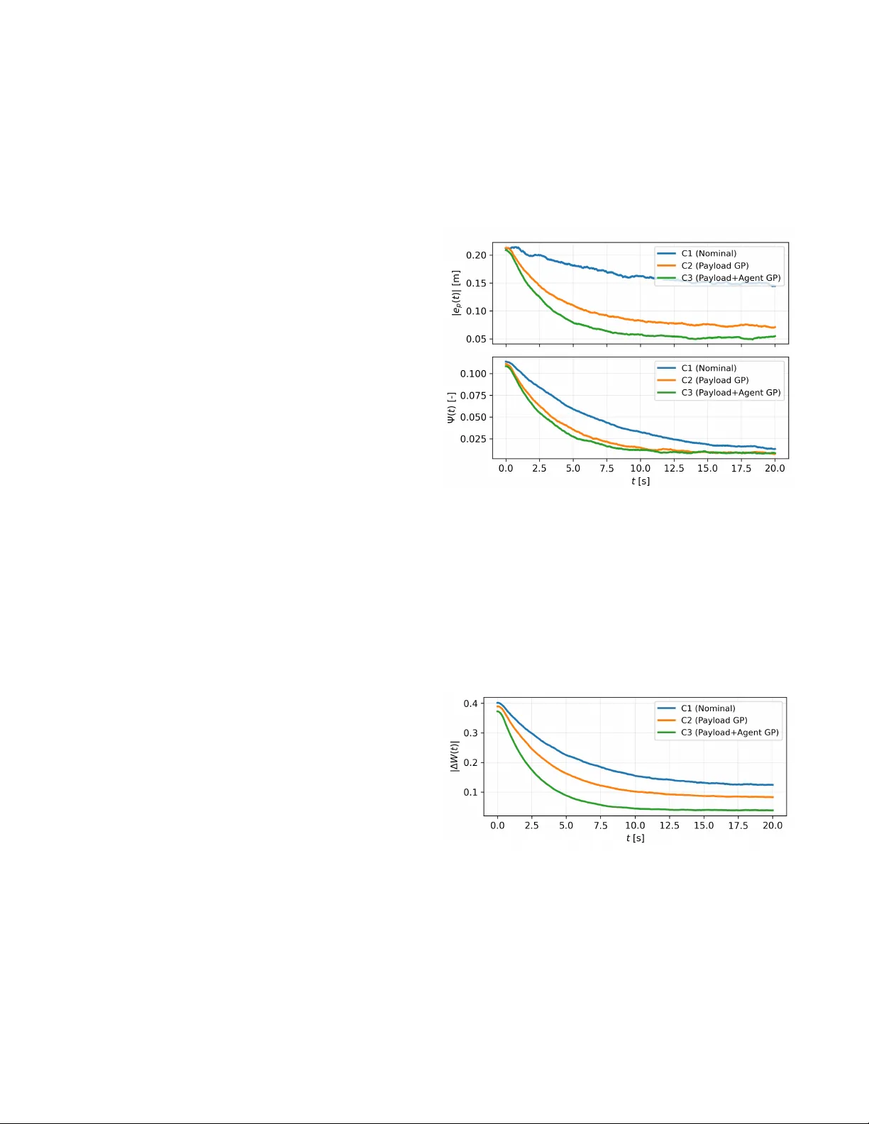
Learning-Based Geometric Leader–Follo wer Control for Cooperati ve Rigid-Payload T ransport with Aerial Manipulators Omayra Y ago Nieto 1 , Leonardo Colombo 2 Abstract — This paper presents a learning-based tracking control framework for cooperative transport of a rigid payload by multiple aerial manipulators under rigid grasp constraints. A unified geometric model is developed, yielding a coupled agent–payload differential–algebraic system that explicitly cap- tures contact wr enches, payload dynamics, and internal f orce redundancy . A leader–f ollower architecture is adopted in which a designated leader generates a desired payload wrench based on geometric tracking errors, while the r emaining agents realize this wrench through constraint-consistent for ce allocation. Unknown disturbances and modeling uncertainties are compensated using Gaussian Process (GP) regr ession. High- probability bounds on the learning error ar e explicitly incor - porated into the control design, combining GP feedforward compensation with geometric feedback. L yapunov analysis es- tablishes uniform ultimate boundedness of the payload tracking errors with high pr obability , with an ultimate bound that scales with the GP predicti ve uncertainty . I . I N T RO D U C T I O N Cooperativ e aerial transportation of large or heavy pay- loads has attracted significant attention in recent years due to its rele vance to inspection, construction, logistics, and disaster-response applications [1], [2]. Compared to single- vehicle aerial manipulation, cooperativ e transport increases payload capacity and robustness through redundancy , but introduces challenging coordination requirements and tightly coupled agent–payload dynamics. These challenges are am- plified under rigid grasp constraints, where contact forces, internal-force redundancy , and payload dynamics must be handled consistently within the control architecture. Early approaches relied on simplified load models (e.g., cable-suspended or quasi-static payloads), enabling decen- tralized or consensus-based strategies [3], [4]. More recent works address rigid payloads grasped by multiple aerial v ehi- cles, which require explicit wrench allocation and constraint handling [5], [6]. Geometric control on S E (3) is particularly effecti ve in this setting, as they provide singularity-free tracking laws for translation and attitude [7], [8]. Despite this progress, most controllers presume accurate knowledge of vehicle and payload dynamics. In practice, co- operativ e aerial manipulation is af fected by model mismatch, 1 Omaya Y ago Nieto is with Universidad Polit ´ ecnica de Madrid, Spain. omayra.yago.nieto@alumnos.upm.es 2 L. Colombo is with Centre for Automation and Robotics (CSIC-UPM), Ctra. M300 Campo Real, Km 0,200, Arganda del Rey - 28500 Madrid, Spain. leonardo.colombo@csic.es The author acknowledge financial support from Grant PID2022- 137909NB-C21 funded by MCIN/AEI/ 10.13039/501100011033. The re- search leading to these results was supported in part by iRoboCity2030-CM, Rob ´ otica Inteligente para Ciudades Sostenibles (TEC-2024/TEC-62), funded by the Programas de Actividades I+D en T ecnolog ´ ıas en la Comunidad de Madrid. aerodynamic disturbances, and uncertain or time-varying payload properties, which can degrade tracking performance and jeopardize grasp consistency . Learning-based augmenta- tion is therefore appealing to compensate unmodeled effects while retaining analytic guarantees. Gaussian Process (GP) regression is especially attractiv e due to its nonparametric modeling capability and uncertainty quantification [9]–[12], but e xtending GP-based guarantees to rigidly grasped cooper - ativ e transport is nontrivial because of holonomic constraints, internal-force redundancy , and agent–payload coupling. This paper de velops a learning-augmented geometric tracking framew ork for cooperative transport of a rigid payload by multiple aerial manipulators under rigid grasp constraints. W e adopt a hierarchical leader–follo wer archi- tecture: a leader generates a desired payload wrench from geometric tracking errors, while the remaining agents real- ize this wrench through constraint-consistent allocation and regulate internal forces. Learning is incorporated via GP regression to compensate unkno wn disturbances with explicit high-probability error bounds used directly in the control design and stability analysis. The paper provides: (i) a unified geometric model lead- ing to coupled agent–payload D AE dynamics with explicit contact wrenches and rigid grasp constraints; (ii) a leader– follower wrench generation/allocation scheme that handles internal-force redundancy under thrust-direction underactu- ation; and (iii) a GP-augmented controller with a L ya- punov analysis establishing high-probability uniform ulti- mate boundedness of the payload tracking errors. The remainder of the paper is as follo ws. Section II deriv es the geometric model and coupled dynamics. Section III sum- marizes the GP learning model and error bounds. Section IV presents the controller and stability analysis. Section V reports simulation results, and Section VI concludes. I I . S Y S T E M M O D E L I N G : S I N G L E A N D C O O P E R AT IV E A E R I A L M A N I P U L A T O R S This section dev elops a unified geometric model, from a single aerial manipulator to multi-agent and rigid-payload coupled dynamics. W e first present the multibody Lie-group formulation, then derive the reduced thrust-based transla- tional dynamics used for learning and control, and finally introduce the cooperativ e and payload-coupled extensions. A. Aerial manipulator as a multibody system. W e consider a multirotor U A V consisting of n +1 in- terconnected rigid bodies arranged in a tree structure. Let R ∈ S O (3) and denote by so (3) its Lie algebra. W e use the standard hat/vee maps ˆ ( · ) : R 3 → so (3) and ( · ) ∨ : so (3) → R 3 . The configuration of the i th body is g i ∈ S E (3) , written as g i =  R i x i 0 1  , where R i ∈ S O (3) and x i ∈ R 3 are the attitude and center-of-mass position. The body twist is ξ i ∈ se (3) with matrix form ξ i =  ˆ ω i v i 0 0  , where ω i , v i ∈ R 3 . The manipulator configuration is described by joint co- ordinates r ∈ R n r and joint torques τ r ∈ R n r , where n r is the number of manipulator joint DoF . W e use base variables q 0 = ( R 0 , x 0 , r ) and ξ 0 = ( ω 0 , v 0 , ˙ r ) , where v 0 = ˙ x 0 . Let g i = g 0 g 0 i ( r ) denote the relativ e transform from the base to body i . The multibody kinetic energy induces a configuration-dependent mass matrix M 0 ( r ) in base coordinates (see, e.g., [13]), which we partition as M 0 ( r ) =   J ( r ) C ( r ) ⊤ M ω ˙ r ( r ) C ( r ) mI 3 M v ˙ r ( r ) M ω ˙ r ( r ) ⊤ M v ˙ r ( r ) ⊤ M ˙ r ˙ r ( r )   , (1) where m := P n i =0 m i is the total mass. Follo wing [13], define the instantaneous center -of-mass position x := 1 m n X i =0 m i x i ∈ R 3 , and perform the standard change of variables R := R 0 , ω := ω 0 , v := v 0 + 1 m  M v ˙ r ( r ) ˙ r + C ( r ) ω  , (2) which diagonalizes the translational block of the mass ma- trix. W e use the reduced state ¯ q :=  R, x , r , ω , v , ˙ r  . Let e 3 = (0 , 0 , 1) ⊤ and let u > 0 denote the lift magnitude along R e 3 , while τ ∈ R 3 is the body torque acting on the base. The nominal dynamics can be written as m ¨ x = m a g + R e 3 u, ˙ R = R ˆ ω , (3)  ω ˙ r  = ¯ M ( r ) − 1  µ ν  , (4)  ˙ µ ˙ ν  = " µ × ω 1 2 ¯ ξ ⊤ ∂ ¯ M ( r ) ¯ ξ # + " τ − C ( r ) ⊤ e 3 u/m τ r − M v ˙ r ( r ) ⊤ e 3 u/m # , (5) where ¯ ξ := ( ω , ˙ r ) and the reduced mass matrix is ¯ M =  J − C T C /m M ω ˙ r − C T M v ˙ r /m M T ω ˙ r − M T v ˙ r C /m M ˙ r ˙ r − M T v ˙ r M v ˙ r /m  . (6) Here a g ∈ R 3 is the gravitational acceleration expressed in the inertial frame. In realistic scenarios, (3)–(5) are affected by unmodeled and uncertain effects (e.g., aerodynamic forces, actuator dynamics, friction, payload v ariations, and couplings induced by manipulator motion). W e represent these effects by un- known smooth functions of the reduced state ¯ q : f x uk : X → R 3 , f ω uk : X → R 3 , f ˙ r uk : X → R n r , where X ⊆ S O (3) × R 3 × R n r × R 3 × R 3 × R n r . The uncertain dynamics then read m ¨ x = m a g + R e 3 u + f x uk ( ¯ q ) , ˙ R = R ˆ ω , (7)  ω ˙ r  = ¯ M ( r ) − 1  µ ν  , (8)  ˙ µ ˙ ν  = " µ × ω 1 2 ¯ ξ ⊤ ∂ ¯ M ( r ) ¯ ξ # + " τ − C ( r ) ⊤ e 3 u/m τ r − M v ˙ r ( r ) ⊤ e 3 u/m # (9) +  f ω uk ( ¯ q ) f ˙ r uk ( ¯ q )  . B. Cooperative aerial manipulation system W e now write the dynamics of the cooperati ve aerial ma- nipulation system in a unified differential–algebraic equation (D AE) form, explicitly accounting for the rigid payload, the holonomic grasp constraints, and the contact wrenches generated by each aerial manipulator . For each aerial manipulator j ∈ { 1 , . . . , N } , we consider the reduced state ¯ q j = ( q j , ξ j ) = ( R j , x j , r j , ω j , v j , ˙ r j ) , as defined in Section II-A. The payload state is given by q L := ( p L , v L , R L , ω L ) , where v L := ˙ p L . The complete system state is z :=  { ¯ q j } N j =1 , q L  . Each UA V agent j ∈ { 1 , . . . , N } is equipped with n manipulator arms. Each arm b ∈ { 1 , . . . , n } estab- lishes a single rigid contact with the payload. The cor- responding contact forces are denoted by λ j,b ∈ R 3 , and we define the stacked contact force vector λ :=  λ ⊤ 1 , 1 · · · λ ⊤ 1 ,n · · · λ ⊤ N , 1 · · · λ ⊤ N ,n  ⊤ ∈ R 3 N n . Let c L j,b ∈ R 3 be the fixed attachment point expressed in the payload frame, and let p j,b ( q j ) denote the inertial position of the corresponding contact point on U A V j (arm b ). The rigid grasp constraints, for b = 1 , . . . , n and j = 1 , . . . , N , are ϕ j,b ( z ) := p j,b ( q j ) −  p L + R L c L j,b  = 0 . (10) Differentiating twice yields the acceleration-lev el compat- ibility conditions used implicitly in the D AE formulation. Each aerial manipulator obeys the thrust-based reduced dynamics augmented by contact forces: ˙ R j = R j ˆ ω j , (11) m j ¨ x j = m j a g + R j e u j + f x uk,j ( q j , ξ j ) + f c x,j ( λ ) , (12)  ω j ˙ r j  = ¯ M − 1 j ( r j )  µ j ν j  , (13)  ˙ µ j ˙ ν j  =  µ j × ω j 1 2 ¯ ξ ⊤ j ∂ ¯ M j ( r j ) ¯ ξ j  +  τ j − C ⊤ j e u j /m j τ r,j − M ⊤ j,v ˙ r e u j /m j  +  f ω uk,j ( q j , ξ j ) f ˙ r uk,j ( q j , ξ j )  − n X b =1 J c,j,b ( q j ) ⊤ λ j,b , (14) where J c,j,b ( q j ) denotes the contact Jacobian associated with contact ( j , b ) . The term f c x,j ( λ ) represents the contribution of the contact forces to the translational channel, which may be omitted if all contact effects are accounted for in (14). The payload kinematics is gi ven by ˙ p L = v L , where v L ∈ R 3 is the payload linear velocity . The payload is driv en by the net contact wrench and is subject to unmodeled effects: m L ˙ v L = N X j =1 n X b =1 λ j,b + f g ,L + f p uk,L ( p L , v L , R L , ω L ) , (15) J L ˙ ω L + ω L × ( J L ω L ) = N X j =1 n X b =1 c L j,b ×  R ⊤ L λ j,b  + f ω uk,L ( p L , v L , R L , ω L ) . (16) Defining the payload wrench W L = [ F L ; τ L ] ∈ R 6 , the contact forces are mapped to the payload dynamics via the grasp matrix W L = G ( R L ) λ G ( R L ) = " I 3 · · · I 3 \ R L c L 1 , 1 · · · \ R L c L N ,n # ∈ R 6 × 3 N n , where the columns are ordered with the stacking of λ . W e stack the contact forces as λ ∈ R 3 N n and the holonomic constraints as Φ( z ) ∈ R 3 N n . Assuming identical manipulators r j ∈ R n r for all j , the differential state dimen- sion is dim( z ) = N (12 + 2 n r ) + 12 = 12( N + 1) + 2 N n r . Equations (11)–(16), together with the algebraic con- straints (10), define a coupled DAE with 12( N + 1) + 2 N n r differential states and 3 N n algebraic variables λ subject to 3 N n holonomic constraints of the form ˙ z = F ( z , u, λ ) + F uk ( z ) , 0 = Φ( z ) , (17) where Φ( z ) stacks the holonomic grasp constraints. Here u ∈ U is the stacked vector of differential control inputs of all agents, e.g., u = col( u 1 , τ 1 , τ r, 1 , . . . , u N , τ N , τ r,N ) . I I I . L E A R N I N G W I T H G A US S I A N P R O C E S S E S Building on the learning-based tracking frame work in [14], we consider cooperati ve transport of a rigid payload by a team of N U A V agents. The coupled closed-loop model in Section II-B is affected by unknown and unmodeled ef- fects including aerodynamic disturbances, actuator dynamics, manipulator–payload coupling errors, and payload param- eter mismatch. W e model these effects as additiv e, state- dependent, and time-in v ariant generalized disturbance terms on the time scale of interest. For each U A V agent j ∈ { 1 , . . . , N } we consider unkno wn maps f x uk,j , f ω uk,j , f ˙ r uk,j : S E (3) × se (3) → R 3 , acting on the translational, rotational, and joint/momentum dynamics of agent j , ev aluated at the reduced state ¯ q j = ( q j , ξ j ) = ( R j , x j , r j , ω j , v j , ˙ r j ) (with r j ∈ R n r for all j ). In addition, the payload dynamics include unknown force/moment terms f p uk,L , f ω uk,L : S E (3) × se (3) → R 3 , ev aluated at the payload state q L := ( p L , v L , R L , ω L ) . W e denote by ˆ f uk,j ( ¯ q j ) :=    ˆ f x uk,j ( ¯ q j ) ˆ f ω uk,j ( ¯ q j ) ˆ f ˙ r uk,j ( ¯ q j )    , ˆ f uk,L ( q L ) := " ˆ f p uk,L ( q L ) ˆ f ω uk,L ( q L ) # the learned predictors used for feedforward compensation. In the GP setting below , ˆ f uk,j ∈ R 9 and ˆ f uk,L ∈ R 6 are chosen as GP posterior means, with associated predicti ve covariance matrices denoted Σ j ( · ) and Σ L ( · ) . W e introduce time-varying datasets collected during exe- cution. W e consider piecewise-constant datasets over inter- vals t ∈ [ t k , t k +1 ) with 0 = t 0 < t 1 < t 2 < · · · . Let D j ( t ) and D L ( t ) denote the streaming datasets. On each interval [ t k , t k +1 ) we freeze the data at the update time by setting D j,k := D j ( t k ) and D L,k := D L ( t k ) . The corresponding (time-index ed) predictors are denoted ˆ f uk,j,k and ˆ f uk,L,k . For each agent j , define the learning output y j :=  y x j y ω j y ˙ r j  ⊤ ∈ R 9 by rearranging the agent dynamics and subtracting estimated contact contributions. Let ˆ λ j,b ∈ R 3 denote the estimated contact forces at the attachment points c L j,b (payload frame), with j ∈ { 1 , . . . , N } and b ∈ { 1 , . . . , n } , and let ˆ λ denote the corresponding stacked vector . Then we set y x j := m j ¨ x j − m j a g − R j e u j − f c x,j ( ˆ λ ) , y ω j := ˙ µ j − µ j × ω j + C ⊤ j e u j /m j (18) − τ j + n X b =1  J c,j,b ( q j ) ⊤ ˆ λ j,b  (1:3) , y ˙ r j := ˙ ν j − 1 2 ¯ ξ ⊤ j ∂ ¯ M j ( r j ) ¯ ξ j + M ⊤ j,v ˙ r e u j /m j (19) − τ r,j + n X b =1  J c,j,b ( q j ) ⊤ ˆ λ j,b  (4:3+ n r ) . (20) W e assume the contact generalized-force term J c,j,b ( q j ) ⊤ ˆ λ j,b ∈ R 3+ n r is stacked consistently with  µ j ν j  , so that its first 3 components act on the µ j -channel and the remaining n r components act on the ν j -channel. Under the coupled DAE dynamics, these labels satisfy y x j = f x uk,j , y ω j = f ω uk,j , y ˙ r j = f ˙ r uk,j , up to measurement noise and numerical differentiation errors. W e collect streaming data pairs ( ¯ q j ( t ) , ˜ y j ( t )) , where ˜ y j = y j + η j and η j models measurement noise, and define the time-varying dataset D j ( t ) = { ( ¯ q { i } j , ˜ y { i } j ) } N j ( t ) i =1 . (21) On t ∈ [ t k , t k +1 ) we freeze D j,k := D j ( t ) and compute the oracle ˆ f uk,j,k ( · ) = µ j,k ( · | D j,k ) as the GP posterior mean, with covariance Σ j,k ( · ) . Define the payload learning output y L :=  y p L y ω L  ⊤ ∈ R 6 by y p L := m L ˙ v L − N X j =1 n X b =1 ˆ λ j,b − f g ,L , y ω L := J L ˙ ω L + ω L × ( J L ω L ) − N X j =1 n X b =1 c L j,b ×  R ⊤ L ˆ λ j,b  . Then, under the coupled DAE dynamics, y p L = f p uk,L and y ω L = f ω uk,L , up to measurement noise and estimation errors (including ˆ λ and differentiation). Let Q L := R 3 × R 3 × S O (3) × R 3 denote the payload state space, with q L = ( p L , v L , R L , ω L ) ∈ Q L . W e collect the time-varying payload dataset D L ( t ) = { ( q { i } L , ˜ y { i } L ) } N L ( t ) i =1 (22) where ˜ y L = y L + η L . On t ∈ [ t k , t k +1 ) we freeze D L,k := D L ( t ) and compute the oracle ˆ f uk,L,k ( · ) = µ L,k ( · | D L,k ) as the GP posterior mean, with covariance Σ L,k ( · ) . Assumption 1: For each agent j and for the payload, the corresponding training data sets D j ( t ) and D L ( t ) are updated only finitely many times. In particular, there exists a time T end ∈ R ≥ 0 such that, for all t ≥ T end , D j ( t ) = D end j , ∀ j , D L ( t ) = D end L . Let S X ⊂ Z be a compact subset of the coupled agent– payload state space Z := X N × Q L containing the relev ant closed-loop trajectories. Assume that ˆ f uk,j and ˆ f uk,L are continuously differentiable with bounded deriv ati ves on S X . For the stability analysis, we require high-probability bounds on the learning error that depend on the confidence lev el. Assumption 2: For any confidence lev els δ L ∈ (0 , 1) and δ j ∈ (0 , 1) , j ∈ { 1 , . . . , N } , there exist bounded functions ¯ ρ j ( · ; δ j ) : X → R ≥ 0 and ¯ ρ L ( · ; δ L ) : Q L → R ≥ 0 such that, for all z ∈ S X , P  ∥ f uk ,j ( ¯ q j ) − ˆ f uk ,j ( ¯ q j ) ∥ ≤ ¯ ρ j ( ¯ q j ; δ j )  ≥ δ j , ∀ j, (23) P  ∥ f uk ,L ( q L ) − ˆ f uk ,L ( q L ) ∥ ≤ ¯ ρ L ( q L ; δ L )  ≥ δ L . (24) Remark 1: For a single global confidence lev el δ ∈ (0 , 1) , define δ L := 1 − 1 − δ N +1 and δ j := 1 − 1 − δ N +1 , j = 1 , . . . , N . Then, by a union bound, the joint confidence event Ω δ := Ω L ( δ L ) ∩ T N j =1 Ω j ( δ j ) satisfies P (Ω δ ) ≥ δ . (Any other split satisfying (1 − δ L ) + P N j =1 (1 − δ j ) ≤ 1 − δ is admissible.) For each agent j , we model each scalar component of ˜ y j ∈ R 9 by an independent GP with kernel k j ( · , · ) and mean m j,i ( · ) . At an update time t k , let the frozen dataset be D j,k = { ( ¯ q { i } j , ˜ y { i } j ) } N j,k i =1 and stack the training inputs and outputs as X j,k :=  ¯ q { 1 } j , . . . , ¯ q { N j,k } j  , Y ⊤ j,k :=  ˜ y { 1 } j , . . . , ˜ y { N j,k } j  . Assume additiv e i.i.d. Gaussian measurement noise, ˜ y { i } j = y { i } j + ε { i } j with ε { i } j ∼ N (0 , σ 2 j I 9 ) . For a query ¯ q ∗ j , the GP posterior predictive mean and variance for the i -th component are µ j,k,i ( ¯ q ∗ j ) = m j,i ( ¯ q ∗ j ) + k j ( ¯ q ∗ j , X j,k ) ⊤ K − 1 j,k ( Y j,k, : ,i − m j,i ( X j,k )) , σ 2 j,k,i ( ¯ q ∗ j ) = k j ( ¯ q ∗ j , ¯ q ∗ j ) − k j ( ¯ q ∗ j , X j,k ) ⊤ K − 1 j,k k j ( ¯ q ∗ j , X j,k ) , where the Gram matrix K j,k ∈ R N j,k × N j,k has entries ( K j,k ) ℓm = k j ( ¯ q { ℓ } j , ¯ q { m } j ) + σ 2 j δ ℓm , and m j,i ( X j,k ) := [ m j,i ( ¯ q { 1 } j ) , . . . , m j,i ( ¯ q { N j,k } j )] ⊤ . W e define the vector-v alued GP posterior quantities µ j,k ( ¯ q ∗ j ) :=  µ j,k, 1 ( ¯ q ∗ j ) · · · µ j,k, 9 ( ¯ q ∗ j )  ⊤ ∈ R 9 , Σ j,k ( ¯ q ∗ j ) :=diag  σ 2 j,k, 1 ( ¯ q ∗ j ) , . . . , σ 2 j,k, 9 ( ¯ q ∗ j )  ∈ R 9 × 9 . On t ∈ [ t k , t k +1 ) , we use ˆ f uk,j,k ( ¯ q ∗ j ) = µ j,k ( ¯ q ∗ j ) and Σ j,k ( ¯ q ∗ j ) . Similarly , each scalar component of ˜ y L ∈ R 6 is modeled by an independent GP with kernel k L ( · , · ) , mean m L,i ( · ) , and noise v ariance σ 2 L . At update time t k , let D L,k = { ( q { i } L , ˜ y { i } L ) } N L,k i =1 and stack X L,k :=  q { 1 } L , . . . , q { N L,k } L  and Y ⊤ L,k :=  ˜ y { 1 } L , . . . , ˜ y { N L,k } L  . Assume ˜ y { i } L = y { i } L + ε { i } L with ε { i } L ∼ N (0 , σ 2 L I 6 ) . For a query q ∗ L , define µ L,k ( q ∗ L ) ∈ R 6 and Σ L,k ( q ∗ L ) ∈ R 6 × 6 exactly as above (with j 7→ L and dimension 9 7→ 6 ). On t ∈ [ t k , t k +1 ) , we use ˆ f uk,L,k ( q ∗ L ) = µ L,k ( q ∗ L ) and Σ L,k ( q ∗ L ) . Remark 2: The mean functions m j,i and m L,i may incor - porate parametric identification of the unknown terms. In the absence of prior knowledge, they are set to zero. T o connect GP regression with the high-probability error bounds in Assumption 2, we rely on standard results from reproducing kernel Hilbert space (RKHS) theory . Giv en a positiv e definite kernel k : X × X → R , there exists a unique Hilbert space H k of functions f : X → R , called the reproducing kernel Hilbert space associated with k , such that the reproducing property f ( x ) = ⟨ f , k ( x, · ) ⟩ H k holds for all f ∈ H k and x ∈ X [15], [16]. Assumption 3: For each U A V agent j ∈ { 1 , . . . , N } and each scalar output component i ∈ { 1 , . . . , 9 } , the unknown function f uk,j,i belongs to the RKHS H k j induced by the kernel k j , with uniformly bounded norm. Similarly , for the payload-lev el unknown dynamics, each scalar component f uk,L,i , i ∈ { 1 , . . . , 6 } , belongs to the RKHS H k L induced by the kernel k L . That is, there exist constants B j > 0 and B L > 0 such that ∥ f uk,j,i ∥ H k j ≤ B j , ∀ i ∈ { 1 , . . . , 9 } , ∀ j , and ∥ f uk,L,i ∥ H k L ≤ B L , ∀ i ∈ { 1 , . . . , 6 } . Lemma 1 (Adapted fr om [17]): Suppose Assumptions 1 and 3 hold, and that the GP models for the agents and the payload are trained on the (frozen) data sets D end j and D end L , respectiv ely . Let µ j ( · ) , Σ j ( · ) and µ L ( · ) , Σ L ( · ) denote the corresponding terminal GP posterior mean and cov ariance. Then, for any confidence lev els δ j ∈ (0 , 1) and δ L ∈ (0 , 1) , there exist scalars β j ( δ j ) > 0 and β L ( δ L ) > 0 such that, for all z ∈ S X , P  ∥ f uk ,j ( ¯ q j ) − µ j ( ¯ q j ) ∥ ≤ β j ( δ j ) ∥ Σ 1 / 2 j ( ¯ q j ) ∥  ≥ δ j , ∀ j, P  ∥ f uk ,L ( q L ) − µ L ( q L ) ∥ ≤ β L ( δ L ) ∥ Σ 1 / 2 L ( q L ) ∥  ≥ δ L . Here β j ( δ j ) ∈ R 9 and β L ( δ L ) ∈ R 6 are vectors with components ( β j ( δ j )) i := s 2 B 2 j + 300 γ j,i ln 3  N j + 1 1 − δ 1 / 9 j  , (25) ( β L ( δ L )) i := s 2 B 2 L + 300 γ L,i ln 3  N L + 1 1 − δ 1 / 6 L  , (26) where B j and B L are the RKHS norm bounds from Assump- tion 3, N j and N L denote the number of training points in the corresponding frozen datasets, and γ j,i , γ L,i are the (maximum) information gains associated with the chosen kernels (defined as in [17]). Pr oof: This is a direct consequence of the standard GP uniform error bound for RKHS-bounded functions (see, e.g., [17, Thm. 6]), applied componentwise to the agent outputs ( 9 scalars) and payload outputs ( 6 scalars), and then stacked into the vector inequalities (23)–(24). Remark 3: Lemma 1 implies Assumption 2 by set- ting ¯ ρ j ( ¯ q j ; δ j ) := ∥ β j ( δ j ) ⊤ Σ 1 / 2 j ( ¯ q j ) ∥ and ¯ ρ L ( q L ; δ L ) := ∥ β L ( δ L ) ⊤ Σ 1 / 2 L ( q L ) ∥ on S X . I V . L E A R N I N G - BA S E D T R A C K I N G C O N T R O L A. Contr ol objective and leader–follower ar c hitectur e W e consider cooperativ e transport of a rigid payload by a team of N aerial manipulators subject to the dynamics (17). The control goal is inherently hier ar chical : at the upper le vel, we seek to track a smooth, time-varying reference trajectory for the payload pose ( p L ( t ) , R L ( t )) ∈ S E (3) with bounded tracking errors in the presence of model uncertainties, exter - nal disturbances, and manipulator–payload coupling effects. At the lower le vel, we require each aerial manipulator to robustly realize the assigned contact forces and the induced base motion imposed by the rigid grasp constraints, so that the applied contact forces remain close to the commanded ones despite agent-lev el uncertainties. This two-layer viewpoint is essential because the payload wrench is generated only through contact interactions: while the allocation layer can compute commanded contact forces consistent with the grasp map, the full D AE is driv en by the forces actually applied by the agents. By explicitly enforc- ing constraint-consistent realization at the agent level, we prev ent disturbances and unmodeled dynamics of individual manipulators from corrupting the net payload wrench via realization errors, thereby enabling a cascade analysis of the coupled closed-loop system. The payload dynamics ev olve on S E (3) and require control of a six-dimensional wrench consisting of a resultant force and moment. Individual aerial manipulators do not act directly on the payload wrench; instead, they generate contact forces at fixed attachment points, which collectiv ely determine the payload motion through the grasp matrix. As a result, the grasp map is generally non-injectiv e: the same payload wrench can be produced by different contact-force vectors, whose components in ker G ( R L ) represent internal forces that do not af fect the payload motion. T o address redundancy in a scalable and physically consis- tent manner , we adopt a leader–follower architecture that sep- arates (i) payload-level wrench generation, (ii) contact-lev el wrench allocation, and (iii) agent-le vel wrench realization. This yields a well-posed design that a v oids unnecessary force conflicts, facilitates multi-le vel stability analysis for (17), and enables extensions to learning-based compensation. The leader generates a desired payload wrench W L,d ( t ) =  F L,d ( t ) τ L,d ( t )  ∈ R 6 based on the payload reference trajectory and the measured (or estimated) payload state. In the nominal case, W L,d is designed using standard geometric techniques on S E (3) and depends on payload tracking errors and their deriv ativ es. The term “leader” refers to the coordination role in wrench generation; the leader agent, like all agents, must still realize the resulting contact commands through its local inputs. At the contact-allocation lev el, the team computes commanded contact forces λ cmd ∈ R 3 N n such that G ( R L ) λ cmd = W L,d , where G ( R L ) ∈ R 6 × 3 N n is the grasp matrix. Since this equation is generally underdetermined, the team solves a wrench allocation problem that distributes load among agents while regulating internal forces. Crucially , the D AE is driven by the applied contact forces λ app , which may dif fer from λ cmd due to agent dynamics and disturbances. W e therefore explicitly account for a realization error e λ := λ app − λ cmd and the induced wrench mismatch ∆ W := G ( R L ) λ app − W L,d . This motiv ates learning residual models both at the agent lev el (to reduce realization error) and at the payload le vel (to compensate net unmodeled wrench effects). Unmodeled effects acting on both the payload and the aerial manipulators are compensated using the learned resid- ual models introduced in Section III. Within the hierarchy abov e, learning enters as feedforward corrections both in the leader’ s wrench generation and in each agent’ s local realization layer , without altering the separation between payload objectives and force allocation. B. Nominal payload wrenc h tracking W e design a payload-le vel controller that generates a desired wrench W L,d = [ F L,d ; τ L,d ] ∈ R 6 ensuring expo- nential tracking of the payload position and almost-global exponential tracking of its attitude in the nominal case. Neglecting unknown forces and moments, the payload dynamics are m L ˙ v L = F L + f g ,L , ˙ p L = v L , (27) J L ˙ ω L + ω L × ( J L ω L ) = τ L , (28) where ( F L , τ L ) denotes the net wrench applied to the payload by the aerial manipulators through the rigid grasp, and f g ,L is the gravitational force expressed in the inertial frame. Assumption 4: In the ideal case of exact wrench realiza- tion, the net payload wrench satisfies W L = G ( R L ) λ app = W L,d . Let ( p L,d ( t ) , R L,d ( t )) ∈ S E (3) be a smooth reference trajectory with bounded deriv atives, and define v L,d := ˙ p L,d . Define the translational tracking errors e p := p L − p L,d , e v := v L − v L,d ; and the attitude and angular-velocity errors using the standard S O (3) error maps e R := 1 2  R ⊤ L,d R L − R ⊤ L R L,d  ∨ , e ω := ω L − R ⊤ L R L,d ω L,d . W e also use the attitude error function Ψ( R L , R L,d ) := 1 2 tr  I − R ⊤ L,d R L  . The payload-le vel controller (leader) generates the desired wrench W L,d = [ F L,d ; τ L,d ] as F L,d := m L ¨ p L,d − m L K p e p − m L K v e v − f g ,L , (29) τ L,d := − K R e R − K ω e ω + ω L × ( J L ω L ) − J L  ˆ ω L R ⊤ L R L,d ω L,d − R ⊤ L R L,d ˙ ω L,d  , (30) where K p , K v , K R , K ω are positive definite gain matrices. Under Assumption 4, substituting (29)–(30) into (27)–(28) yields the closed-loop error dynamics ˙ e p = e v , ˙ e v = − K p e p − K v e v , (31) ˙ e R = E ( R L , R L,d ) e ω , (32) J L ˙ e ω = − K R e R − K ω e ω , (33) where E ( · ) is a smooth, bounded matrix depending on e R . The translational error subsystem (31) is exponentially stable. Likewise, the rotational error subsystem (32)–(33) is exponentially stable about e R = e ω = 0 in the standard almost-global sense on S O (3) (see e.g., [7]). C. Nominal trac king contr ol under rigid grasp constraints W e now design a nominal tracking controller for the cooperativ e aerial manipulation system described in Section IV -B, assuming perfect knowledge of the dynamics and neglecting the unkno wn terms f uk,j and f uk,L . Let ( p L,d ( t ) , R L,d ( t )) ∈ S E (3) denote a sufficiently smooth desired payload trajectory , with associated velocities and accelerations ( v L,d , ˙ v L,d , ω L,d , ˙ ω L,d ) , where v L,d := ˙ p L,d and ˙ v L,d := ¨ p L,d . The control objectiv e is to driv e the payload pose to the reference while respecting the rigid grasp constraints (10) and the underactuated nature of the aerial vehicles. Since the number of contact-force variables generally ex- ceeds the wrench dimension, the force allocation problem is redundant and G ( R L ) admits a nontrivial nullspace. Conse- quently , there e xist infinitely many contact-force distrib utions that generate the same payload wrench. The components of λ in ker( G ( R L )) correspond to internal for ces , which do not affect the payload motion but influence grasp tensions, actuator effort, and robustness margins. Partition the grasp matrix as G ( R L ) =  G ℓ ( R L ) G f ( R L )  , where n ℓ ∈ { 1 , . . . , N n } denotes the number of leader contacts (i.e., the number of grasp points assigned to the leader block), so that G ℓ ( R L ) ∈ R 6 × 3 n ℓ collects the columns associated with the leader contacts and G f ( R L ) ∈ R 6 × 3( N n − n ℓ ) collects the remaining columns. Assume the leader grasp block has full row rank, rank( G ℓ ( R L )) = 6 . Accordingly , the leader contact forces are chosen as λ ℓ = G † ℓ ( R L ) W L,d , (34) where G † ℓ denotes a right pseudoin verse chosen so that G ℓ ( R L ) G † ℓ ( R L ) = I 6 . The follower forces are restricted to internal-force directions: λ f = λ f , 0 + N  G f ( R L )  η , λ f , 0 ∈ ker  G f ( R L )  , (35) where N ( G f ( R L )) is a basis matrix for ker( G f ( R L )) and η is a free internal-force input. Lemma 2: Assume rank( G ℓ ( R L )) = 6 and choose the allocation (34)–(35) with λ f , 0 ∈ ker( G f ( R L )) . Then the resulting net payload wrench satisfies W L = G ( R L ) λ = G ℓ ( R L ) λ ℓ + G f ( R L ) λ f = W L,d , (36) independently of the internal-force input η . Pr oof: By the full row-rank assumption, choose G † ℓ such that G ℓ G † ℓ = I 6 . Then (34) gives G ℓ ( R L ) λ ℓ = W L,d . Moreover , (35) with λ f , 0 ∈ ker( G f ( R L )) yields G f ( R L ) λ f = G f ( R L ) λ f , 0 + G f ( R L ) N ( G f ( R L )) η = 0 since G f ( R L ) N ( G f ( R L )) = 0 by definition of a nullspace basis. Hence W L = G ℓ λ ℓ + G f λ f = W L,d . □ Let the holonomic rigid-grasp constraints be stacked as Φ( z ) = 0 as in (10), and define the constraint manifold M := { z ∈ X N × Q L : Φ( z ) = 0 } . Pr oposition 1: Assume the D AE (17) is re gular on M , in the sense that for ev ery ( z , u ) ∈ M × U there exists a locally unique multiplier λ = λ ( z , u ) such that the correspond- ing solution satisfies d dt Φ( z ( t )) = 0 . Consider the closed loop obtained by applying the wrench command (29)–(30) together with the allocation (34)–(35) and any smooth agent- lev el inputs u ( t ) compatible with (17). If the initial condition is consistent, i.e., z (0) ∈ M and d dt Φ( z ( t )) | t =0 = 0 , then the corresponding maximal solution remains on the constraint manifold: z ( t ) ∈ M for all t in its interval of existence. Pr oof: Along any dif ferentiable trajectory z ( t ) , differ - entiating the holonomic constraint gi ves d dt Φ( z ( t )) = D Φ( z ( t )) ˙ z ( t ) . Substituting the D AE dynamics yields the constraint- consistency equation 0 = D Φ( z )  F ( z , u, λ ) + F uk ( z )  . By the regularity assumption, for each ( z , u ) ∈ M × U there exists a locally unique λ = λ ( z , u ) such that the above identity holds, hence d dt Φ( z ( t )) = 0 along the resulting solution. Therefore, Φ( z ( t )) is constant on the interval of existence. Since z (0) ∈ M implies Φ( z (0)) = 0 , we obtain Φ( z ( t )) ≡ 0 for all t , i.e., z ( t ) ∈ M . □ Giv en the commanded contact forces λ j,b , each U A V agent j must generate the corresponding body thrust u j and torques ( τ j , τ r,j ) in a manner consistent with the dynamics (11)– (14). The translational objectiv e is implicit: due to the rigid grasp constraints (10), the agents are kinematically forced to follow the payload motion. Accordingly , the individual agent controllers are designed to track the induced base trajectories and to realize the commanded contact forces while respecting thrust-direction underactuation inherent to multirotor platforms. Assumption 5: On each interval t ∈ [ t k , t k +1 ) , the agent- lev el controllers use the frozen GP oracles ˆ f uk,j,k = µ j,k trained on D j,k and yield a bound on the induced payload wrench mismatch ∆ W of the form ∥ ∆ W ( t ) ∥ ≤ α W e − γ W ( t − t k ) ∥ e λ ( t k ) ∥ + ϑ W + N X j =1 κ j ¯ ρ j ( ¯ q j ( t ); δ j ) , (37) for all consistent trajectories in S X , where α W , γ W , κ j ≥ 0 are constants and ϑ W ≥ 0 collects bounded effects due to measurement noise, numerical differentiation, and contact- force estimation. Remark 4: Under Lemma 1, one may choose ¯ ρ j ( ¯ q j ; δ j ) = β j ( δ ) ∥ Σ 1 / 2 j,k ( ¯ q j ) ∥ on S X . Hence (37) makes the payload-le vel disturbance induced by agent uncertainties explicit in terms of the agent GP cov ariances. Under the wrench command (29)–(30), the allocation (34)–(35), and Proposition 1, solutions remain on M and the nominal allocation ensures W L = W L,d whenev er ∆ W ≡ 0 (Lemma 2). In practice, the applied contact forces induce a mismatch ∆ W which is treated through the interface (37) and will be propagated to payload tracking performance in the learning-based analysis below . D. Learning-based trac king contr ol W e now extend the leader–follo wer tracking controller of Section IV -C to the setting where both the U A V agents and the payload are subject to unkno wn and unmodeled dynam- ics, as introduced in Section III. The goal is to preserve bounded tracking performance while explicitly accounting for learning uncertainty in a way that is compatible with the D AE structure (17) and the hierarchical realization. At the payload layer , the leader augments the nominal wrench command with GP-based feedforward compensation of the unknown payload-level force/moment terms. At the agent layer, each UA V uses its own GP model to compensate local unknown dynamics so as to improve contact-force realization. This is consistent with the fact that (i) payload disturbances alone induce disturbances on the agents through the rigid constraints, and (ii) each agent has additional, local uncertainties. Both effects are represented in the coupled model and are addressed by learning. T o keep the analysis modular , we treat the agent layer through an input-to-state interface: agent-le vel uncertainties affect the payload only via the wrench mismatch ∆ W in- duced by the contact-force realization error e λ . The payload- lev el GP then compensates residual unknown wrench terms acting directly on the payload. Let ˆ f uk,L ( q L ) = µ L,k ( q L ) denote the frozen GP posterior mean on t ∈ [ t k , t k +1 ) , with cov ariance Σ L,k ( q L ) , where q L = ( p L , v L , R L , ω L ) . W e define the learning-augmented virtual payload wrench W L,d = [ F L,d ; τ L,d ] as F L,d := m L ˙ v L,d − m L K p e p − m L K v e v − f g ,L − ˆ f p uk,L,k ( q L ) , (38) τ L,d := − K R e R − K ω e ω + ω L × ( J L ω L ) − ˆ f ω uk,L,k ( q L ) − J L  ˆ ω L R ⊤ L R L,d ω L,d − R ⊤ L R L,d ˙ ω L,d  , (39) where K p , K v , K R , K ω are symmetric positive definite gain matrices and the learned terms are ev aluated at the current payload state. The allocation layer remains unchanged: W L,d is mapped to commanded contact forces λ cmd via (34)–(35). Define the learning errors (frozen on [ t k , t k +1 ) ) as ˜ f L,k ( q L ) := f uk,L ( q L ) − ˆ f uk,L,k ( q L ) = " ˜ f p L,k ( q L ) ˜ f ω L,k ( q L ) # . Substituting (38)–(39) and  F L τ L  = G ( R L ) λ app = W L,d + ∆ W into the payload error dynamics yields m L ˙ e v = − m L K p e p − m L K v e v + ∆ F + ˜ f p L,k ( q L ) , (40) J L ˙ e ω = − K R e R − K ω e ω + ∆ τ + ˜ f ω L,k ( q L ) , (41) where ∆ W = [∆ F ; ∆ τ ] . W e now establish a tracking guarantee that explicitly accounts for (i) learning uncertainty through Σ L,k and (ii) the agent-layer realization mismatch through ∆ W . Theor em 1: Suppose Assumptions 1, 2, and 3 hold. Con- sider the learning-augmented payload wrench (38)–(39) com- bined with the allocation (34)–(35). Assume the agent-layer interface in Assumption 5 holds. Then, for any confidence lev el δ ∈ (0 , 1) , the pay- load tracking errors ( e p , e v , e R , e ω ) are uniformly ultimately bounded with probability at least δ on S X . Moreov er , up to a decaying transient from (37), the ultimate bound scales proportionally to ¯ ρ L ( q L ; δ ) + N X j =1 ¯ ρ j ( ¯ q j ; δ ) + ϑ W . Pr oof: Fix an update interval t ∈ [ t k , t k +1 ) and split the global confidence lev el δ into δ L , δ 1 , . . . , δ N . Define the confidence event Ω δ := n ∥ ˜ f L,k ( q L ( t )) ∥ ≤ ¯ ρ L ( q L ( t ); δ L ) , ∥ f uk ,j ( ¯ q j ( t )) − ˆ f uk ,j,k ( ¯ q j ( t )) ∥ ≤ ¯ ρ j ( ¯ q j ( t ); δ j ) o (42) ∀ j, ∀ t ≥ 0 . By Assumption 2 and the union bound (Re- mark 1), P (Ω δ ) ≥ δ on S X . Consider the L yapunov function V ( e p , e v , e R , e ω ) := 1 2 m L ∥ e v ∥ 2 + 1 2 m L e ⊤ p K p e p + 1 2 e ⊤ ω J L e ω + 1 2 e ⊤ R K R e R . Along trajectories on the constraint manifold M we have ˙ e p = e v and ˙ e R = E ( R L , R L,d ) e ω for a smooth bounded matrix E ( · ) . Using (40)–(41) and cancelling cross terms yields ˙ V = − m L e ⊤ v K v e v − e ⊤ ω K ω e ω + e ⊤ v (∆ F + ˜ f p L,k ) + e ⊤ ω (∆ τ + ˜ f ω L,k ) ≤ − k v ∥ e v ∥ 2 − k ω ∥ e ω ∥ 2 + ∥ ( e v , e ω ) ∥  ∥ ∆ W ∥ + ∥ ˜ f L,k ( q L ) ∥  , (43) where k v := m L λ min ( K v ) and k ω := λ min ( K ω ) . On Ω δ , ∥ ˜ f L,k ( q L ) ∥ ≤ ¯ ρ L ( q L ; δ ) , hence ˙ V ≤ − k ∥ ( e v , e ω ) ∥ 2 + ∥ ( e v , e ω ) ∥  ∥ ∆ W ∥ + ¯ ρ L ( q L ; δ )  , (44) with k := min { k v , k ω } . Applying Y oung’ s inequality , for any ε ∈ (0 , k ) , ∥ ( e v , e ω ) ∥  ∥ ∆ W ∥ + ¯ ρ L ( q L ; δ L )  ≤ ε ∥ ( e v , e ω ) ∥ 2 + 1 4 ε  ∥ ∆ W ∥ + ¯ ρ L ( q L ; δ L )  2 . (45) Combining (44) and (45) gi ves ˙ V ≤ − ( k − ε ) ∥ ( e v , e ω ) ∥ 2 + 1 4 ε  ∥ ∆ W ∥ + ¯ ρ L ( q L ; δ L )  2 , on Ω δ . (46) Next we use the agent-layer interface (Assumption 5) on [ t k , t k +1 ) . Define the decaying transient χ k ( t ) := α W e − γ W ( t − t k ) ∥ e λ ( t k ) ∥ , t ∈ [ t k , t k +1 ) , and the aggregated uncertainty lev el Ξ( t ) := ¯ ρ L ( q L ( t ); δ L ) + ϑ W + N X j =1 κ j ¯ ρ j ( ¯ q j ( t ); δ j ) + χ k ( t ) . Then ∥ ∆ W ( t ) ∥ + ¯ ρ L ( q L ( t ); δ L ) ≤ Ξ( t ) and (44) implies ˙ V ≤ − ( k − ε ) ∥ ( e v , e ω ) ∥ 2 + 1 4 ε Ξ( t ) 2 on Ω δ . (47) Finally , relate ∥ ( e v , e ω ) ∥ 2 to V . Since V ≥ 1 2 m L ∥ e v ∥ 2 + 1 2 λ min ( J L ) ∥ e ω ∥ 2 , there exists c 1 > 0 such that ∥ ( e v , e ω ) ∥ 2 ≥ c 1 V for all ( e p , e v , e R , e ω ) . Thus, for some constants c 2 , c 3 > 0 , ˙ V ≤ − c 2 V + c 3 Ξ( t ) 2 on Ω δ . By the comparison lemma, for all t ∈ [ t k , t k +1 ) , V ( t ) ≤ e − c 2 ( t − t k ) V ( t k ) + c 3 Z t t k e − c 2 ( t − s ) Ξ( s ) 2 ds. Since S X is compact, ¯ ρ L ( · ; δ ) and ¯ ρ j ( · ; δ ) are bounded on S X , and χ k ( t ) decays exponentially . Therefore the integral term is uniformly bounded and yields a uniform ultimate bound. Moreover , up to the exponentially decaying tran- sient χ k ( t ) , the ultimate bound scales with ¯ ρ L ( q L ; δ L ) + P N j =1 ¯ ρ j ( ¯ q j ; δ j ) + ϑ W . □ Remark 5: Under Lemma 1, on the confidence ev ent Ω δ one may choose ¯ ρ L ( q L ; δ L ) = β L ( δ L ) ∥ Σ 1 / 2 L,k ( q L ) ∥ and ¯ ρ j ( ¯ q j ; δ j ) = β j ( δ j ) ∥ Σ 1 / 2 j,k ( ¯ q j ) ∥ , ∀ j , for all q L , ¯ q j ∈ S X . Hence, up to the decaying transient in (37), the ul- timate tracking accuracy in Th. 1 scales with the GP predictiv e uncertainties at the payload and agent states β L ( δ )   Σ 1 / 2 L,k ( q L )   + N X j =1 β j ( δ )   Σ 1 / 2 j,k ( ¯ q j )   + ϑ W , and im- prov es monotonically as the cov ariances contract with ad- ditional data. Remark 6: The proposed learning-based controller admits a clear robustness–performance trade-off. The GP mean provides feedforward compensation of unknown dynamics, while the predictiv e covariance quantifies the remaining model mismatch and determines the high-probability track- ing accuracy . In parallel, improved contact-force realization reduces ∆ W , tightening the ultimate bound without altering the leader–follower structure. ⋄ Cor ollary 1: Under the assumptions of Theorem 1, fix δ ∈ (0 , 1) and split it into δ L , δ 1 , . . . , δ N as in Remark 1. If, along a sequence of learning updates k → ∞ , the predictiv e cov ariance satisfies sup q L ∈ S X   Σ 1 / 2 L,k ( q L )   → 0 , and the agent-layer mismatch satisfies sup t ≥ 0 ∥ ∆ W k ( t ) ∥ → 0 , then the ultimate bound in Theorem 1 conv er ges to zero on Ω δ . Consequently , in the limit k → ∞ the learning-based closed loop recovers the nominal asymptotic tracking behavior . Pr oof: Fix δ ∈ (0 , 1) and work on the ev ent Ω δ (so that all GP error bounds inv oked in Theorem 1 hold uniformly on S X , with confidence lev els δ L for the payload and δ j for the agents). From Theorem 1, there exist class- K L and class- K functions β ( · , · ) and γ ( · ) and a nonnegati v e term χ k ( t ) (the decaying transient from (37)) such that, for all t ≥ 0 , ∥ ( e p , e v , e R , e ω )( t ) ∥ ≤ β ( ∥ ( e p , e v , e R , e ω )(0) ∥ , t ) + γ  ¯ d k  + χ k ( t ) , (48) where the effecti ve disturbance level ¯ d k can be chosen as ¯ d k := sup q L ∈ S X ¯ ρ L,k ( q L ; δ L ) + sup t ≥ 0 ∥ ∆ W k ( t ) ∥ + ϑ W , (49) (here ¯ ρ L,k denotes the payload GP high-probability error radius on update interval k ). By Lemma 1, on Ω δ we may take ¯ ρ L,k ( q L ; δ L ) = β L ( δ L ) ∥ Σ 1 / 2 L,k ( q L ) ∥ , hence sup q L ∈ S X ¯ ρ L,k ( q L ; δ L ) ≤ β L ( δ L ) sup q L ∈ S X ∥ Σ 1 / 2 L,k ( q L ) ∥ − → 0 . By assumption, sup t ≥ 0 ∥ ∆ W k ( t ) ∥ → 0 as k → ∞ . There- fore, from (49) we obtain ¯ d k → ϑ W . If ϑ W = 0 (idealized case with no measurement/estimation artifacts), then ¯ d k → 0 and (48) implies that the ultimate b ound γ ( ¯ d k ) conv erges to zero, i.e., the closed loop recovers the nominal asymptotic tracking behavior as k → ∞ . If ϑ W > 0 , then the ultimate bound conv erges to γ ( ϑ W ) , i.e., performance is limited only by the non-learning artifacts captured by ϑ W . □ V . S I M U L A T I O N R E S U L T S Next, we validate the hierarchical learning-based leader– follower architecture for cooperative rigid-payload transport. The simulations are designed to: (i) verify payload track- ing under rigid grasp constraints using the coupled agent– payload D AE (17), (ii) isolate the roles of payload-lev el and agent-lev el learning within the two-layer realization view- point of Section IV -A, and (iii) connect the observed tracking accuracy to the high-probability UUB bound of Theorem 1, which depends on the payload GP uncertainty , the agent GP uncertainties, and the agent-to-payload realization interface through the induced wrench mismatch ∆ W . W e consider a team of N = 2 aerial manipulators cooper- ativ ely transporting a rigid payload. Each agent establishes n = 2 rigid contacts with the payload, yielding a total of N n = 4 contacts and a stacked contact-force v ector λ ∈ R 12 . The coupled dynamics are simulated using the full agent– payload DAE model, including constraint reactions and contact wrenches. The payload reference ( p L,d ( t ) , R L,d ( t )) consists of a smooth position trajectory with bounded deriv a- tiv es and a constant desired attitude. This excites the trans- lational dynamics while keeping the rotational ev aluation interpretable through ∥ e R ( t ) ∥ and ∥ e ω ( t ) ∥ . T o emulate realistic mismatch and external effects, we introduce: (i) parametric mismatch in payload mass and inertia (controller uses nominal ( m L , J L ) different from the true values), (ii) additiv e unknown force/torque disturbances acting directly on the payload dynamics, and (iii) local agent- lev el unmodeled effects affecting contact-force realization (e.g., unmodeled aerodynamic terms and input biases). In addition, measurement noise and numerical differentiation are included in the force reconstruction pipeline, producing a bounded realization floor captured by the constant ϑ W in Assumption 5. All simulations start from consistent initial conditions on the constraint manifold M . Each agent is assumed to hav e access to estimates of the contact forces λ j,b via model-based force ob- servers (disturbance/unknown-input observers) or residual- based force estimation using onboard state estimates and actuator models. W e denote by λ cmd the commanded contact forces produced by the allocation layer and by λ app the applied/realized forces. The agent-to-payload interface signal is the induced wrench mismatch ∆ W ( t ) which dri ves the payload as an additiv e disturbance in (40)–(41). W e compare three controller configurations under identical initial conditions and reference trajectories: • Case (C1) Nominal (no learning): the learning terms are disabled at both layers, i.e., ˆ f uk,L ≡ 0 and ˆ f uk,j ≡ 0 . • Case (C2) Payload learning: the leader uses the payload GP compensation ˆ f uk,L,k = µ L,k in (38)–(39), while the agents do not use GP compensation, i.e., ˆ f uk,j ≡ 0 . • Case (C3) P ayload+agent learning: both the leader and each agent use their respective GP compensators, ˆ f uk,L,k = µ L,k and ˆ f uk,j,k = µ j,k , improving contact- force realization and thereby reducing ∆ W . In all cases, the allocation layer is identical and uses (34)– (35). Thus, differences between (C2) and (C3) reflect the effect of agent-layer learning on the disturbance ∆ W . W e report the payload tracking errors ∥ e p ( t ) ∥ , ∥ e v ( t ) ∥ , ∥ e R ( t ) ∥ , and ∥ e ω ( t ) ∥ , together with the interface signal ∥ ∆ W ( t ) ∥ . T o connect to Theorem 1, we also plot the pre- dictiv e standard deviations along the closed-loop trajectories: σ L ( t ) := ∥ Σ 1 / 2 L,k ( q L ( t )) ∥ , σ A ( t ) := P N j =1 ∥ Σ 1 / 2 j,k ( ¯ q j ( t )) ∥ . On the confidence e vent used in Assumption 2 and Lemma 1, the theorem indicates that, up to a decaying transient due to the realization dynamics, the ultimate tracking accuracy scales with a combination of ¯ ρ L ( q L ; δ ) , P j ¯ ρ j ( ¯ q j ; δ ) , and ϑ W . Accordingly , we examine how reductions in σ L ( t ) and σ A ( t ) correlate with reductions in tracking error and ∥ ∆ W ( t ) ∥ . The GP prior uses a squared-exponential (RBF) cov ari- ance with automatic relev ance determination (ARD), i.e., one characteristic length-scale per input coordinate, and an additiv e i.i.d. white-noise term. W e fit independent scalar GPs per output channel: 6 GPs for the payload residual (one per wrench component) using the 20 -dimensional payload feature vector , and 9 GPs per agent for the agent-le vel residual using the corresponding agent feature vector . In both cases, the kernel h yperparameters (signal v ariance, ARD length-scales, and noise variance) are learned by maximizing the log marginal likelihood on the associated frozen dataset. Large learned length-scales (near the imposed upper bound) indicate weak sensitivity to the associated feature, whereas smaller values identify the most informativ e coordinates for predicting the disturbance residual. Figure 1 reports the position error norm ∥ e p ( t ) ∥ and the attitude error measure Ψ( t ) for (C1)–(C3). All cases remain bounded and exhibit transient decay follo wed by nonzero ul- timate le vels due to residual uncertainties. Compared with the nominal case (C1), enabling payload learning (C2) reduces the steady tracking offset by compensating the ef fecti ve payload-lev el unkno wn wrench. Adding agent learning (C3) further tightens the ultimate bound by improving contact- force realization and thereby reducing the induced mismatch ∆ W , in agreement with Theorem 1. Fig. 1. Payload tracking on S E (3) for (C1)–(C3). T op: position error norm ∥ e p ( t ) ∥ . Bottom: attitude error measure Ψ( t ) . Ultimate bounds decrease from (C1) to (C2) to (C3), consistent with Theorem 1. Figure 2 plots ∥ ∆ W ( t ) ∥ . The reduction from (C2) to (C3) highlights the role of agent-layer learning: improving contact-force realization reduces the ef fecti ve disturbance entering the payload error dynamics. This observation sup- ports the modular two-layer design, where agent uncertainties affect payload tracking only through ∆ W . Fig. 2. Payload wrench mismatch ∥ ∆ W ( t ) ∥ for (C1)–(C3). Agent learning reduces the interface disturbance entering the payload error dynamics. Figure 3 shows the predictiv e standard deviations σ L ( t ) and σ A ( t ) ev aluated along the closed-loop trajectories. Regions of larger predictive uncertainty correlate with larger transient tracking errors, while better-cov ered regions (smaller variance) yield tighter tracking. These trends are consistent with the high-probability residual bounds used in Lemma 1 and Theorem 1. Fig. 3. Uncertainty measures along the closed-loop trajectory for (C1)– (C3). T op: payload-le vel uncertainty σ L ( t ) decreases when payload learning is enabled (C2–C3). Bottom: agent-level uncertainty σ A ( t ) decreases only when agent learning is enabled (C3); thus σ A ( t ) remains essentially unchanged from (C1) to (C2). Fig. 4. Norms of the estimated applied contact forces for each agent. The forces remain bounded throughout the maneuver and show no high- frequency chattering. The bottom panel shows the internal-force input magnitude ∥ η ( t ) ∥ ; when activated, η redistributes contact forces along internal directions without affecting the net payload wrench (Lemma 2). Figure 4 reports the norms of the estimated applied contact forces for each agent. Across all cases, the force magnitudes remain bounded over the maneuver and do not exhibit high- frequency chattering, indicating that the allocation and real- ization layers yield a well-conditioned contact-force behav- ior . When the internal-force input η is activ ated (see ∥ η ( t ) ∥ ), the contact-force distribution is reshaped along internal-force directions while preserving the commanded payload wrench, in agreement with Lemma 2. Future work will focus on a full experimental implementa- tion on a multi-U A V testbed with rigid grasping, including (i) real-time force reconstruction/estimation for λ j,b and online computation of ∆ W , (ii) onboard GP training/inference with incremental data management and update scheduling, (iii) allocator and realization layers with actuator/tilt/thrust saturation handling and safety constraints on contact forces and internal-force inputs, and (iv) systematic identification of the disturbance sources (aerodynamics, actuator dynamics, payload parameter drift) to build informative feature vectors and improve generalization across operating conditions. R E F E R E N C E S [1] D. Mellinger and V . Kumar , “Minimum snap trajectory generation and control for quadrotors, ” IEEE International Confer ence on Robotics and Automation , pp. 2520–2525, 2011. [2] M. Ryll, H. H. B ¨ ulthoff, and P . R. Giordano, “Modeling and control of a quadrotor uav with tilting propellers, ” in 2012 IEEE international confer ence on robotics and automation . IEEE, 2012, pp. 4606–4613. [3] J. R. Goodman, T . Beckers, and L. J. Colombo, “Geometric control for load transportation with quadrotor uavs by elastic cables, ” IEEE T ransactions on Contr ol Systems T echnolo gy , vol. 31, no. 6, pp. 2848– 2862, 2023. [4] N. Michael, J. Fink, and V . Kumar , “Cooperative manipulation and transportation with aerial robots, ” Autonomous Robots , vol. 30, no. 1, pp. 73–86, 2011. [5] A. Ollero, M. T ognon, A. Suarez, D. Lee, and A. Franchi, “Past, present, and future of aerial robotic manipulators, ” IEEE T ransactions on Robotics , vol. 38, no. 1, pp. 626–645, 2021. [6] Z. W ang, S. Singh, M. Pav one, and M. Schwager , “Cooperative object transport in 3d with multiple quadrotors using no peer communi- cation, ” in 2018 IEEE International Conference on Robotics and Automation (ICRA) . IEEE, 2018, pp. 1064–1071. [7] T . Lee, M. Leok, and N. H. McClamroch, “Geometric tracking control of a quadrotor uav on SE(3), ” IEEE T ransactions on Control Systems T echnolo gy , vol. 18, no. 3, pp. 671–688, 2010. [8] K. Sreenath, T . Lee, and V . Kumar , “Geometric control and differential flatness of a quadrotor uav with a cable-suspended load, ” IEEE Confer ence on Decision and Contr ol , pp. 2269–2274, 2013. [9] C. E. Rasmussen and C. K. I. Williams, Gaussian Pr ocesses for Machine Learning . MIT Press, 2006. [10] F . Berkenkamp, A. P . Schoellig, and A. Krause, “Safe model-based reinforcement learning with stability guarantees, ” Advances in Neural Information Processing Systems , vol. 30, 2017. [11] T . Beckers, S. Hirche, and L. Colombo, “Online learning-based formation control of multi-agent systems with gaussian processes, ” in 2021 60th IEEE Confer ence on Decision and Control (CDC) . IEEE, 2021, pp. 2197–2202. [12] T . Beckers, L. J. Colombo, S. Hirche, and G. J. Pappas, “Online learning-based trajectory tracking for underactuated vehicles with uncertain dynamics, ” IEEE Contr ol Systems Letters , vol. 6, pp. 2090– 2095, 2021. [13] M. K obilarov , “Trajectory control of a class of articulated aerial robots, ” IEEE International Conference on Unmanned Aircr aft Systems (ICU AS) , 2013. [14] O. Y ago Nieto and L. Colombo, “Safe learing-based control for an aerial robot with manipulator arms, ” IF A C-P apersOnLine , vol. 58, no. 6, pp. 36–41, 2024. [15] G. W ahba, Spline Models for Observational Data , ser . CBMS-NSF Regional Conference Series in Applied Mathematics. Philadelphia, P A: SIAM, 1990, vol. 59. [16] I. Steinwart and A. Christmann, Support vector machines . Springer Science & Business Media, 2008. [17] N. Srinivas, A. Krause, S. M. Kakade, and M. W . Seeger , “Information-theoretic regret bounds for Gaussian process optimiza- tion in the bandit setting, ” IEEE T ransactions on Information Theory , vol. 58, no. 5, pp. 3250–3265, May 2012.