Pilot-Free Optimal Control over Wireless Networks: A Control-Aided Channel Prediction Approach

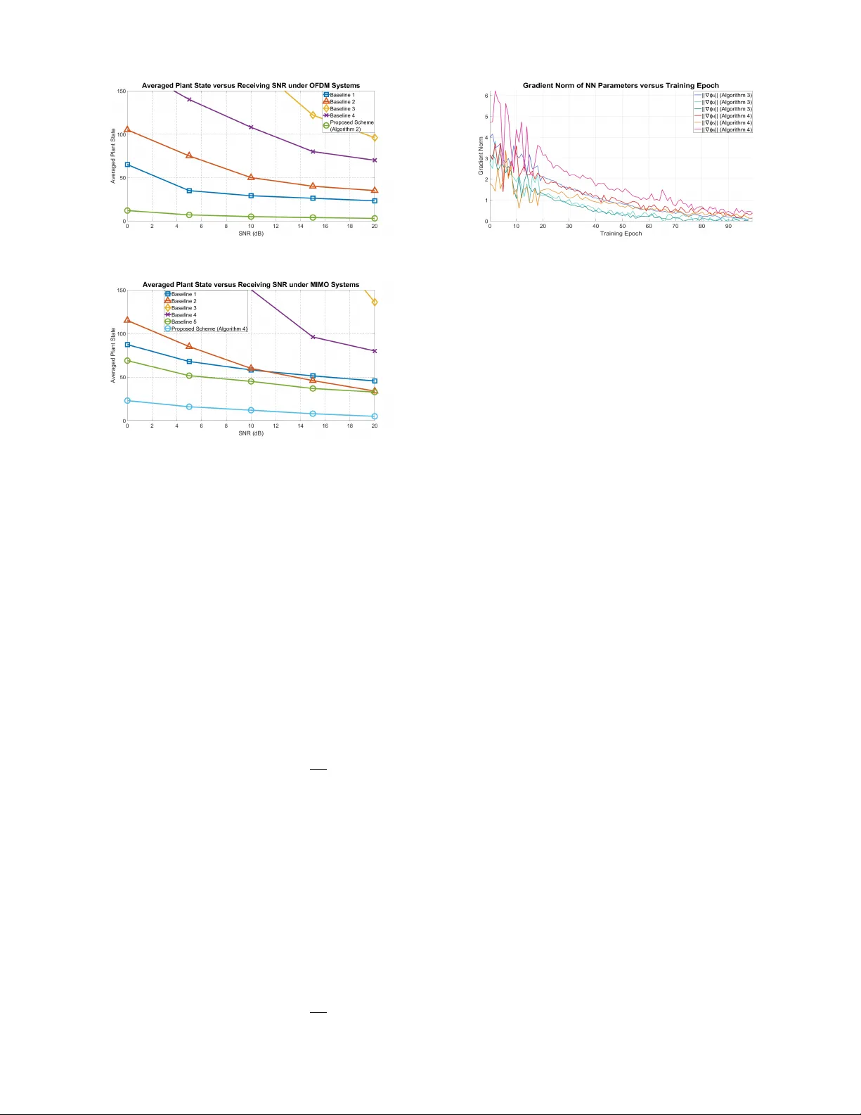
1 Pilot-Free Optimal Control o v er W ireless Networks: A Control-Aided Channel Prediction Approach Minjie T ang, Member , IEEE , Zunqi Li, Graduate Student Member , IEEE , Photios A. Stavrou, Senior Member , IEEE , and Marios K ountouris, F ellow , IEEE Abstract —A recurring theme in optimal contr oller design f or wireless networked control systems (WNCS) is the reliance on real-time channel state information (CSI). However , acquiring accurate CSI a priori is notoriously challenging due to the time- varying nature of wireless channels. In this work, we propose a pilot-free framework for optimal control over wireless channels in which control commands ar e generated from plant states together with control-aided channel pr ediction. For linear plants operating over an orthogonal frequency-di vision multiplexing (OFDM) architecture, channel prediction is performed via a Kalman ﬁlter (KF), and the optimal contr ol policy is deri ved from the Bellman principle. T o alleviate the curse of dimensionality in computing the optimal control policy , we approximate the solution using a coupled algebraic Riccati equation (CARE), which can be computed efﬁciently via a stochastic approximation (SA) algorithm. Rigorous performance guarantees are estab- lished by proving the stability of both the channel predictor and the closed-loop system under the resulting control policy , pro viding sufﬁcient conditions for the existence and uniqueness of a stabilizing approximate CARE solution, and establishing con vergence of the SA-based control algorithm. The framework is further extended to nonlinear plants under general wireless architectur es by combining a KalmanNet-based predictor with a Markov-modulated deep deterministic policy gradient (MM- DDPG) controller . Numerical results show that the proposed pilot-free approach outperforms benchmark schemes in both control performance and channel prediction accuracy for linear and nonlinear scenarios. Index T erms —Pilot-free communication, optimal control, rein- for cement learning, system stability , channel prediction. I . I N T R O D U C T I O N A. Backgr ound T HE rapid advances in 5G wireless networks and edge computing have accelerated the development of wireless networked control systems (WNCSs), in which feedback loops are closed over wireless communication links [1]. Owing to their ﬂexibility , scalability , and ease of deployment, WNCSs hav e been adopted in a wide range of applications, including autonomous driving [2], cooperati ve unmanned aerial vehicle (U A V) swarms [3], and the industrial Internet of Things (IIoT) [4]. A typical WNCS consists of a (potentially un- stable) dynamic plant equipped with co-located actuators, a Minjie T ang and Photios A. Stavrou are with the Department of Communication Systems, EURECOM, France (e-mail: { minjie.tang, fo- tios.stavrou } @eurecom.fr). Zunqi Li is with the School of Electronics and Information Engineering, Harbin Institute of T echnology , Harbin, China (e- mail: lizunqi@stu.hit.edu.cn). Marios Kountouris is with the Department of Communication Systems, EURECOM, France, and the Department of Computer Science and Artiﬁcial Intelligence, Uni versity of Granada, Spain (kountour@eurecom.fr; mariosk@ugr .es). remote controller , and a time-v arying wireless link between the controller and the actuator (cf. Fig. 1). The remote controller receiv es real-time state feedback and generates intermittent control commands, which are transmitted over the wireless channel to the actuator and applied to stabilize the plant. Closing the loop ov er a wireless medium inevitably introduces communication impairments, such as fading and noise, that can degrade control performance and jeopardize stability . From a control-design standpoint, it is therefore desirable to adapt the control policy to the instantaneous channel conditions, which requires accurate channel state information (CSI). In practice, ho wev er , acquiring timely and reliable CSI is challenging due to the fast time variation of wireless channels and the overhead associated with channel probing. This moti vates the following question: Can we design an optimal contr oller without a priori CSI? B. Prior Art Most existing controller -design approaches for WNCSs are dev eloped under static or otherwise simpliﬁed communica- tion assumptions, primarily for linear plants. For example, proportional-integral-deri v ativ e (PID) control has been widely used in networked settings [5]–[7], but its heuristic nature typically requires extensi ve tuning. More systematic methods, such as linear quadratic regulation (LQR) [8], [9] and model predictiv e control (MPC) [10]–[12], provide principled designs for linear systems; howe ver , they commonly assume ideal, static, or perfectly known communication channels. When deployed ov er wireless links, their performance can deteriorate and stability may be compromised due to channel uncertainty . T o improv e robustness, sev eral works adopt simpliﬁed ran- dom channel models, including additiv e white Gaussian noise (A WGN) [13], packet drops [14], [15], and ﬁnite-state Marko v packet-loss models [16]–[18]. While these models facilitate analysis and synthesis, they do not capture key character- istics such as multipath of practical fading channels. More recent studies consider control ov er fading links [19]–[21], but typically rely on further simpliﬁcations such as independent and identically distributed (i.i.d.) fading [19], [20] or ﬁnite- state Markov fading models [21], [22]. Such models neglect temporal correlation and the continuous, high-dimensional channel states induced by multipath propagation. In addition, most of the abo ve literature focuses on linear plants. Extending linear designs to nonlinear dynamics in a brute-force manner can lead to instability or substantial performance degradation. Finally , many existing approaches assume that the controller 2 Fig. 1: T ypical WNCS architecture under the proposed pilot-free framework. has access to perfect CSI, which is difﬁcult to guarantee in time-varying wireless en vironments due to channel-estimation latency and pilot overhead. Accurate CSI typically requires explicit channel acquisition (e.g., estimation or prediction). Con ventional approaches are predominantly pilot-aided [23]–[25]: the transmitter (the re- mote controller in our setting) sends kno wn pilot sequences so that the receiver (the actuator) can estimate the channel, after which the estimated CSI is fed back for transmitter- side processing (e.g., controller design). While effecti ve, pilot- aided acquisition incurs non-negligible spectral and energy ov erhead, which becomes especially burdensome in massiv e multiple-input multiple-output (MIMO) systems. Moreover , pilot contamination due to the reuse of non-orthogonal pilots across users or antennas can signiﬁcantly degrade estimation accuracy and limit scalability . T o reduce pilot overhead, a vari- ety of alternati ves hav e been e xplored, including blind [26] and semi-blind methods [27], compressed sensing approaches [28], and deep learning-based techniques [29]. Blind and semi- blind methods exploit statistical or structural properties of the transmitted signals, but often suffer from slow con vergence, high computational complexity , and sensitivity to modeling assumptions. Compressed sensing lev erages channel sparsity to reduce the number of measurements, but its performance depends critically on the validity of the sparsity model and can be fragile in the presence of noise and model mis- match. Deep learning-based approaches can capture nonlinear channel dynamics and temporal correlations; howe ver , they typically require large amounts of labeled training data that are generated using pilots, which reintroduces substantial ofﬂine ov erhead and may limit adaptability to changing channel conditions. T o design controllers for nonlinear plants, a v ariety of methods have been proposed. Classical nonlinear control tech- niques, including feedback linearization [30]–[32], adaptiv e control [33], and sliding-mode control [34], often require restrictiv e structural assumptions on the dynamics (e.g., input– output decoupling, matched uncertainty , or linear parameteriz- ability). Such conditions can be difﬁcult to satisfy in complex en vironments with strong nonlinearities and uncertainty , which limits the applicability of these approaches. More recently , reinforcement learning (RL)-based methods [35], [36] hav e gained attention because they can learn policies through interaction, without imposing explicit parametric forms on the nonlinear dynamics. Nev ertheless, most existing RL-based controllers are developed under idealized [35] or simpli- ﬁed [36] communication models (e.g., i.i.d. packet drops). In addition, they often assume access to instantaneous CSI, which is difﬁcult to obtain reliably in practical WNCSs with fast time-varying channels. In contrast to existing works that assume either perfect CSI or exogenous channel acquisition mechanisms, the present pa- per considers a fundamentally different information structure in which the channel state is not directly observed and no dedicated probing is av ailable. Instead, channel knowledge must be inferred from the closed-loop interaction between control actions and plant state transitions. This endogenous information acquisition mechanism couples channel prediction and system control in a non-separable manner and leads to a covariance-dependent Riccati recursion and stability condi- tions that differ from classical linear quadratic Gaussian (LQG) or Marko v jump formulations. C. Main Contributions In this work, we dev elop a pilot-free optimal control frame- work for both linear and nonlinear plants operating o ver unreliable wireless fading channels. The proposed framew ork explicitly accounts for temporal channel correlation and high- dimensional channel states induced by multipath propagation, providing a more faithful model of practical wireless en- vironments. The main idea is to exploit control signals to simultaneously re gulate the plant and enable contr ol-aided channel pr ediction fr om real-time state observations , thereby av oiding the need for a priori CSI. The main contributions are summarized as follo ws: 1) Pilot-free WNCS framework. W e propose a pilot-fr ee framew ork for WNCSs. In contrast to prior work that typically treats controller design and channel acquisition separately and assumes that CSI is either perfectly known or obtained via dedicated pilot transmissions [5]–[11], our framew ork reuses real-time control commands as implicit pilots to facilitate channel prediction. T o the best of our knowledge, this is the ﬁrst approach that le verages control signals directly for channel prediction in WNCSs. This paradigm enables controller design without a priori CSI, reducing pilot ov erhead while maintaining strong control performance. 2) Pilot-free optimal control for linear OFDM systems. W e study a pilot-free optimal control problem for linear plants o ver an orthogonal frequency-division multiplexing (OFDM) architecture. W e formulate coupled problems for channel prediction and system control. The optimal predictor is characterized by a Kalman ﬁlter (KF) [37], 3 while the optimal control policy follows from the Bell- man optimality principle [38]. T o mitigate the curse of dimensionality in solving the resulting continuous- state Bellman equation, we dev elop a tractable approx- imation via statistical quantization and interpret the ap- proximate solution through a coupled algebraic Riccati equation (CARE). The CARE is computed using an online stochastic-approximation (SA) algorithm [39] that exploits control-aided channel prediction. W e establish performance guarantees by proving: (i) mean-square sta- bility of the channel prediction process and stability of the closed-loop plant, (ii) sufﬁcient conditions for the existence and uniqueness of a stabilizing approximate CARE solution, and (iii) almost sure con vergence of the proposed SA-based algorithm. 3) Extension to nonlinear plants under general wireless architectur es. W e extend the pilot-free framework to nonlinear plants operating over general communication models, including MIMO, orthogonal time frequency space (OTFS) [40], and afﬁne frequency division mul- tiplexing (AFDM) [41] architectures. In this setting, we employ KalmanNet [42] for channel prediction and a Marko v-modulated deep deterministic policy gradient (MM-DDPG) method [43] for system control. T o the best of our knowledge, this is the ﬁrst work to integrate KalmanNet for channel prediction in nonlinear WNCSs. Compared with extended and unscented Kalman ﬁlters, KalmanNet av oids Jacobian and sigma-point computa- tions and does not require exact noise statistics, while retaining a model-aware structure that improves robust- ness under strong nonlinearities and model mismatch. Moreov er , MM-DDPG explicitly incorporates the pre- dicted Markovian channel state into the control policy update, enabling stable channel-adapti ve system control in continuous, high-dimensional action spaces. Notation: Uppercase and lowercase boldface letters denote matrices and vectors, respectiv ely . The operators ( · ) T , ( · ) H and T r( · ) denote the transpose, Hermitian transpose, and trace, respecti vely . The symbol 0 m × n and 0 m denote an m × n matrix and m × m all-zero matrices, respectively , and I m represents the m × m identity matrix. For a sequence ( a 1 , . . . , a n ) , Diag( a 1 , . . . , a n ) denotes the diagonal matrix with diagonal entries a 1 , . . . , a n . The sets R m × n and C m × n denote real and complex m × n matrices, respectiv ely; S m + and S m ++ denote the sets of m × m positive semideﬁnite and positiv e deﬁnite matrices, respecti vely; Z + denotes the set of nonnegati ve integers; and R and C denote the sets of real and complex numbers. The norms || A || , ∥ A ∥ F , and || a || denote the spectral norm of a matrix A , the Frobenius norm of A , and the Euclidean norm of a vector a , respectiv ely . The “ ℓ 0 - norms” ∥ A ∥ 0 and ∥ a ∥ 0 count the number of nonzero entries in A and a , respectively . For a matrix A , [ A ] i, : and [ A ] : ,i denote its i th row and i th column, respectively , and for a vector a , [ a ] i denotes its i th entry . I I . S Y S T E M M O D E L This section presents the proposed pilot-free architecture for the WNCS. W e consider a linear dynamical system operating ov er an OFDM-based wireless network, as illustrated in Fig. 1. A. Decision-Making at the Dynamic Plant The physical plant in Fig. 1 typically inv olves many spa- tially distributed state variables that capture their temporal ev olution. For example, in a chemical process, the state may include temperature, humidity , and concentration at different locations; in an aircraft, it may include atmospheric pressure, airspeed, and engine thrust. Their dynamics are commonly modeled by ﬁrst-order coupled linear difference equations of the form x k +1 = Ax k + B b u k + w k , k = 0 , 1 , 2 , . . . , (1) where x k ∈ C S × 1 denotes the plant state at time slot k , with initial condition x 0 ∼ C N ( 0 S × 1 , σ 2 x I S ) . The vector b u k ∈ C N × 1 denotes the receiv ed (noise-contaminated) control command. Moreover , A ∈ R S × S and B ∈ R S × N are the internal plant dynamics and actuation (input) matrices, respectiv ely , and the pair ( A , B ) is assumed controllable. The process noise w k ∼ C N ( 0 S × 1 , W ) is additive with ﬁnite cov ariance W ∈ S S + . B. Signal Generation and T ransmission at the Remote Con- tr oller Follo wing Fig. 1, the remote controller monitors the plant state history x k 0 = { x 0 , . . . , x k } using a depth-of-ﬁeld (DoF) camera, and simultaneously predicts the wireless channel based on the observed states x k 0 and the control command history u k − 1 0 = { u 0 , . . . , u k − 1 } . The predicted fading matrix for time slot k + 1 , given information up to slot k , is denoted by b H ( k + 1 | k ) = f pred ( x k 0 , u k − 1 0 ) , (2) where f pred ( · ) is the channel prediction operator, whose form depends on the adopted prediction strategy and will be speciﬁed in Sections III and IV. The prediction b H ( k + 1 | k ) ∈ C N × N is modeled as a diagonal matrix constructed from the predicted complex fading vector b h ( k + 1 | k ) = ([ b h ( k + 1 | k )] 1 , . . . , [ b h ( k + 1 | k )] N ) T ∈ C N , where [ b h ( k + 1 | k )] i ∈ C denotes the predicted fading gain on subcarrier i . Accordingly , b H ( k + 1 | k ) = Diag( b h ( k + 1 | k )) . The control command u k is generated based on the plant state history x k 0 and the predicted channel gain b H ( k + 1 | k ) , as follo ws 1 u k = f cont ( x k 0 , b H ( k + 1 | k )) , (3) where f cont ( · ) denotes the control policy , which will be speci- ﬁed in Section III and Section IV. By incorporating b H ( k + 1 | k ) into the control policy design f cont ( · ) , the resulting control command u k ∈ C N × 1 adapts to wireless fading conditions, thereby improving the reliability of closed-loop regulation. Although b H ( k + 1 | k ) is obtained from the history { x k 0 , u k − 1 0 } through the channel prediction module, we explicitly treat x k 1 As will be shown in Section III, the information structure of u k in (3) is deriv ed from the solution to Problem 2 and depends only on the current plant state x k , rather than on the entire plant-state history x k 0 . 4 and b H ( k + 1 | k ) as distinct inputs to f cont ( · ) . This choice is consistent with the modular architecture in Fig. 1. The control command u k is then mapped onto prede- termined subcarriers in the frequency domain, yielding the frequency-domain transmit vector s f k ∈ C N × 1 . W e adopt a ﬁxed, disjoint subcarrier assignment in which each control component [ u k ] i is mapped to exactly one unique subcarrier (i.e., without overlap). The resulting subcarrier allocation is described by a binary matrix P ∈ { 0 , 1 } N × N , which satisﬁes the follo wing constraints: • Bandwidth utilization constraint: ∥ P ∥ 0 = N . This enforces full utilization of the available subcarriers. • Disjoint mapping constraint: [ P ] T : ,i [ P ] : ,j = 0 N × N for all i  = j , where i, j ∈ { 1 , . . . , N } . This guarantees that distinct control components are assigned to nonoverlap- ping subcarriers. • Bijectiv e mapping constraint: ∥ [ P ] : ,i ∥ 0 = 1 and ∥ [ P ] j, : ∥ 0 = 1 for all i, j ∈ { 1 , . . . , N } . Hence, each control component [ u k ] i is mapped to exactly one sub- carrier , and each subcarrier is used by exactly one control component. The frequency-domain symbol vector s f k ∈ C N × 1 is con- verted into a time-domain block ˜ s t k ∈ C N × 1 via the in verse fast Fourier transform (IFFT), i.e., ˜ s t k = F H s f k , (4) where F ∈ C N × N denotes the unitary discrete Fourier transform (DFT) matrix. T o mitigate intersymbol interference induced by multipath propagation, a cyclic preﬁx (CP) of length L cp is appended by copying the last L cp samples of ˜ s t k to the beginning of the block, yielding s t k =  ˜ s t k,N − L cp +1 , . . . , ˜ s t k,N , ˜ s t k, 1 , . . . , ˜ s t k,N  T , (5) where s t k ∈ C ( N + L cp ) × 1 denotes the CP-extended transmit vector . After CP insertion, s t k is con verted from parallel to serial and undergoes radio-frequency (RF) processing prior to transmission ov er the wireless channel to the plant. C. Signal Reception at the Dynamic Plant Follo wing Fig. 1, the received serial time-domain wav eform is ﬁrst con verted into a parallel block via serial-to-parallel (S/P) con version. The resulting receiv ed vector is b s t k = H t k +1 s t k + n t k , (6) where H t k +1 ∈ C ( N + L cp ) × ( N + L cp ) is the T oeplitz con volution matrix induced by the channel impulse response h t k +1 = [ h t 0 ,k +1 , . . . , h t L h − 1 ,k +1 ] T ∈ C L h × 1 . Here, L h denotes the ef- fectiv e channel length (i.e., the number of signiﬁcant multipath taps), and n t k ∼ C N ( 0 N + L cp , σ 2 n I N + L cp ) is the A WGN in the time domain. After discarding the ﬁrst L cp samples corresponding to the cyclic preﬁx, the effecti ve N -sample receiv ed vector is b s r k = R b s t k = H circ k +1 ˜ s t k + ˜ n t k , (7) where R ∈ { 0 , 1 } N × ( N + L cp ) is a selection matrix that remov es the CP by extracting the last N samples of the receiv ed block. The matrix H circ k +1 ∈ C N × N denotes the resulting circulant conv olution matrix induced by h t k +1 (i.e., H circ k +1 = RH t k +1 R T under the CP-length condition), and ˜ n t k ∼ C N ( 0 N × 1 , σ 2 n I N ) is the A WGN vector after CP remov al. Applying the Fast Fourier T ransform (FFT) to b s r k giv es 2 b s f k = F b s r k = H k +1 s f k + n k , (8) where F ∈ C N × N is the unitary DFT matrix (implemented via an FFT) and n k ∼ C N ( 0 N × 1 , σ 2 n I N ) is the frequency- domain A WGN. The frequency-domain channel matrix is H k +1 = FH circ k +1 F H = Diag( h 1 ,k +1 , . . . , h N ,k +1 ) ∈ C N × N , which is diagonal since H circ k +1 is circulant. 3 Each subcarrier gain h i,k +1 ∈ C ev olves according to the Gauss-Markov process [44] h i,k +1 = αh i,k + p 1 − α 2 v i,k , (9) where α ∈ [ − 1 , 1] is the temporal correlation coefﬁcient and v i,k ∼ C N (0 , σ 2 v ) is i.i.d. circularly symmetric complex Gaussian noise. The initial condition is h i, 0 ∼ C N (0 , 1) . Beyond the frequency-domain structure, the temporal ev o- lution of each subcarrier is modeled by the Gauss-Marko v process in (9), where the correlation coefﬁcient α satisﬁes α ∈ [ − 1 , 1] . This condition is physically reasonable: values | α | > 1 would lead to an unstable channel recursion with unbounded average channel power , implying unrealistically large receiv ed power (and hence SNR) over time. As a rep- resentativ e special case for isotropic scattering with a moving terminal, Clarke’ s model gives α = J 0 (2 π f D T s ) , where J 0 ( · ) is the Bessel function of the ﬁrst kind of order zero, f D is the maximum Doppler frequency , and T s is the sampling interval. Since J 0 ( z ) is bounded for all real z (with range approximately [ − 0 . 4028 , 1] ), the condition α ∈ [ − 1 , 1] is always satisﬁed in practice. The plant then recov ers the control command b u k ∈ C N × 1 from the recei ved frequenc y-domain signal b s f k as b u k = P T b s f k = H c k +1 u k + n c k , (10) where H c k +1 = P T H k +1 and n c k = P T n k . The recov ered control command b u k is subsequently applied to the plant dynamics gi ven in (1), as discussed in Section II-A. D. Pilot-F ree Communication P aradigm for the WNCS The models in Sections II-A - II-C highlight a pilot-free communication paradigm for WNCSs, in which the control signal u k plays a dual role: it driv es the plant dynamics and 2 W e assume that the plant state x k ∈ C S × 1 , the control signal u k ∈ C N × 1 , the received control input b u k ∈ C N × 1 , and the channel fading matrices H k , H c k ∈ C N × N are all complex-valued, in order to capture the complex baseband representation of wireless transmissions (see, e.g., [23]–[26]). This modeling captures both amplitude attenuation and phase rotation induced by multipath fading. Unlike much of the existing WNCS literature (see, e.g., [17]–[19]), which assumes real-valued signals throughout, our formulation provides a more faithful representation of practical wireless en vironments. 3 In Section IV, we extend the framework to general communication architectures in which H k +1 is not necessarily diagonal, and the control components [ u k ] i and [ u k ] j , for i  = j and i, j ∈ { 1 , . . . , N } , may become correlated cross subcarriers during transmission. 5 simultaneously provides information for implicit prediction of the channel H k +1 through the relationship among x k , u k , and its noise-corrupted observation b u k . Speciﬁcally , the remote controller generates u k from the current plant state x k and the predicted channel b H ( k + 1 | k ) via (3), while the prediction of H k +1 is performed using the history of control signals u k − 1 0 and state trajectories x k 0 via (2). In contrast to con ventional WNCS designs (see, e.g., [19]–[21], which assume perfect CSI or rely on dedicated pilot transmission to support controller design), the proposed pilot-free approach reuses the control signals for channel prediction, thereby reducing signaling ov erhead and improving spectral and energy ef ﬁciency . In the following sections, we detail the design of the control signal u k in (3) and the channel predictor b H ( k + 1 | k ) in (2) under the proposed pilot-fr ee framework. I I I . L I N E A R S Y S T E M S OV E R O F D M In this section, we develop methods to design the channel prediction operator f pred ( x k 0 , u k − 1 0 ) in (2) and the control policy f cont ( x k , b H ( k + 1 | k )) in (3) for a linear plant operating ov er an OFDM communication architecture. A. Pr oblem F ormulation W e seek to jointly improve channel-prediction accuracy for the time-v arying channel gains { H c 1 , H c 2 , . . . } and the effecti veness of control inputs { u 0 , u 1 , . . . } so as to enhance closed-loop plant stability . Speciﬁcally , the channel prediction polic y π p = { b H (1 | 0) , b H (2 | 1) , . . . } aims to accurately predict the channel sequence { H c 1 , H c 2 , . . . } appearing in (10). This objective is formalized by the following optimization problem. Problem 1 (Channel Prediction) . min π p (1) – (10) lim sup K →∞ 1 K K − 1 X k =0 E h c p ( b H ( k + 1 | k ) , H c k +1 ) | x k 0 , u k − 1 0 i , wher e the per -stage cost is deﬁned as c p ( b H ( k + 1 | k ) , H c k +1 ) ≜   b H ( k + 1 | k ) − H c k +1   2 F . (11) The control policy π c = { u 0 , u 1 , . . . } aims to stabilize the dynamic plant over the wireless link, which leads to the following optimization problem. Problem 2 (Optimal Control) . min π c (1) – (10) lim sup K →∞ 1 K K − 1 X k =0 E [ c d ( x k , u k )] , (12) with per-sta ge cost c d ( x k , u k ) ≜ x H k Qx k + u H k Ru k , (13) wher e Q ∈ S S ++ and R ∈ S N ++ ar e positive deﬁnite weighting matrices that penalize the state deviation and contr ol effort, r espectively . Remark 1 (Coupling Between Problems 1 and 2) . Although Pr oblems 1 and 2 are stated separately , the y ar e inher ently coupled in the pr oposed pilot-fr ee framework. In particular , as will be shown in Section III-C, the solution to Pr oblem 2 depends on the pr edicted channel b H ( k + 1 | k ) , which is pr oduced by solving Pr oblem 1. B. Solution to Pr oblem 1 Optimal solution and algorithm implementation. The optimal solution to Problem 1 is gi ven by the minimum mean-square error (MMSE) predictor of H c k +1 at each time slot, i.e., b H ( k + 1 | k ) = arg min b H ( k +1 | k ) E [ ∥ b H ( k + 1 | k ) − H c k +1 ∥ 2 F | x k 0 , u k − 1 0 ] . T o deriv e an explicit MMSE predictor , we combine the plant dynamics in (1) with the control-reception model in (10), which yields the follo wing channel-observ ation relation: x k = Ax k − 1 + BU k − 1 h c k + Bn c k − 1 + w k − 1 , (14) where U k = Diag ([ u k ] 1 , . . . , [ u k ] N ) ∈ C N × N denotes the diagonal matrix formed from the control input, and h c k = [[ H c k ] 1 , 1 , [ H c k ] 2 , 2 , . . . , [ H c k ] N ,N ] H ∈ C N × 1 collects the (diagonal) subcarrier gains. Moreov er , the channel evolution in (9) can be written compactly in vector form as h c k +1 = α h c k + v k , (15) where v k ∈ C N × 1 collects the innov ation terms, with entries [ v k ] i = √ 1 − α 2 v i,k for i ∈ { 1 , . . . , N } . Note that (15) speciﬁes a linear state-ev olution model for h c k , while (14) provides a linear observation model for h c k . Consequently , Problem 1 reduces to an MMSE prediction problem for the vectorized channel gain h c k , which can be solved optimally via a KF as follows Deﬁne: b h ( k | k ) ≜ E [ h c k | x k 0 , U k − 1 0 ] , (16) b h ( k | k − 1) ≜ E [ h c k | x k − 1 0 , U k − 2 0 ] , (17) Σ( k | k ) ≜ E [( h c k − b h ( k | k ))( h c k − b h ( k | k )) H | x k 0 , U k − 1 0 ] , (18) Σ( k | k − 1) ≜ E [( h c k − b h ( k | k − 1))( h c k − b h ( k | k − 1)) H | x k − 1 0 , U k − 2 0 ] , (19) where b h ( k | k ) , b h ( k | k − 1) ∈ C N × 1 denote the posterior estimate and prior prediction of the vectorized channel gain h c k , respectiv ely , and Σ( k | k ) , Σ( k | k − 1) ∈ S N + are the corresponding posterior and prior error covariance matrices. Assume that the initial channel prediction satisﬁes b h (1 | 0) ∼ C N ( 0 N × 1 , I N ) . Then, the optimal solution to Problem 1 is the MMSE predictor b H ( k + 1 | k ) = arg min b H E [ ∥ b H − H c k +1 ∥ 2 F | x k 0 , u k − 1 0 ] = Diag([ b h ( k + 1 | k )] 1 , . . . , [ b h ( k + 1 | k )] N ) , (20) where b h ( k + 1 | k ) is the one-step lookahead Kalman prediction produced by Algorithm 1. Remark 2 (Equi valence of MMSE Prediction for H c k and h c k ) . Ther e is a one-to-one correspondence between the diagonal matrix H c k and the vector h c k . Speciﬁcally , h c k collects the 6 Algorithm 1 Channel Prediction in Linear OFDM Systems Under the Pilot-Free Frame work 1: Initialization: 2: Set initial prior error cov ariance Σ(1 | 0) = I N 3: Set b h (1 | 0) ∼ C N ( 0 N × 1 , Σ(1 | 0)) 4: for k = 1 , 2 , . . . do 5: Construct U k − 1 = Diag([ u k − 1 ] 1 , . . . , [ u k − 1 ] N ) , 6: where u k − 1 is provided by Algorithm 2 7: • Estimation Step (f or h c k ): 8: Compute the Kalman gain 9: K k = Σ( k | k − 1) U H k − 1 B T ( BU k − 1 Σ( k | k − 1) 10: U H k − 1 B T + σ 2 n BB T + W  − 1 , 11: Update the posterior estimate 12: b h ( k | k ) = b h ( k | k − 1) + K k ( x k − Ax k − 1 − BU k − 1 13: × b h ( k | k − 1)  , 14: Update the posterior error cov ariance 15: Σ( k | k ) = ( I N − K k BU k − 1 )Σ( k | k − 1) 16: × ( I N − K k BU k − 1 ) H + K k ( σ 2 n BB T + W ) K H k . 17: • Prediction Step (for h c k +1 ): 18: b h ( k + 1 | k ) = α b h ( k | k ) , 19: Σ( k + 1 | k ) = α 2 Σ( k | k ) + V , 20: where V = σ 2 υ Diag(1 − α 2 , ..., 1 − α 2 ) ∈ C N × N . 21: end for diagonal entries of H c k , and H c k = Diag( h c k ) . Therefor e, MMSE pr ediction of H c k is equivalent to MMSE pr ediction of h c k . T o implement Algorithm 1, we follo w the standard KF recursion. Speciﬁcally , at each time slot k , the algorithm consists of two steps: • Estimation step: Update the posterior channel estimate b h ( k | k ) and the associated error cov ariance Σ( k | k ) using the observed state transition { x k , x k − 1 } and the applied control input u k − 1 . • Prediction step: Propagate the posterior estimate using the channel dynamics in (15) to obtain the one-step prediction b h ( k + 1 | k ) and its error cov ariance Σ( k + 1 | k ) . As a result, Algorithm 1 provides both the one-step looka- head channel prediction b H ( k + 1 | k ) and the ﬁltered channel estimate b H ( k | k ) at each time slot. Channel prediction stability . W e next analyze the perfor- mance of Algorithm 1, with a particular focus on its long-term channel prediction stability , as characterized in the following theorem. Theorem 1 (Stability of Channel Prediction) . Under the pr oposed pilot-fr ee contr ol framework, suppose the channel state evolves accor ding to the linear dynamics (15) and is r elated to the plant evolution thr ough the linear observation model (14) . Then, the one-step lookahead channel pr ediction err or covariance Σ( k +1 | k ) gener ated by Algorithm 1 is mean- squar e stable, in the sense that lim sup K →∞ 1 K K − 1 X k =0 E [T r(Σ( k + 1 | k ))] ≤ σ 2 υ N 1 − α 2 1 | α | < 1 + N 1 | α | =1 < ∞ . (21) Pr oof: The channel recursion in (15) is time-inv ariant. For | α | < 1 , it admits a stationary distribution with lim k →∞ h c k ∼ C N (0 , σ 2 υ 1 − α 2 I N ) , whereas for | α | = 1 the channel power does not contract, and we have h c k = h c 0 ∼ C N ( 0 , I N ) , ∀ k = 0 , 1 , ... Consider ﬁrst the degenerate case with no observ ations, i.e., u k = 0 N × 1 for all k , so that BU k = 0 and the Kalman recursion reduces to pure prediction. Then the prediction error covariance satis- ﬁes lim sup k →∞ Σ( k + 1 | k ) = σ 2 υ 1 − α 2 I N 1 | α | < 1 + I N 1 | α | =1 and therefore lim sup k →∞ T r(Σ( k + 1 | k )) = N σ 2 υ 1 − α 2 1 | α | < 1 + N 1 | α | =1 . When u k  = 0 N × 1 for some time slots, the predic- tion performance improves relative to the no-observation case. Fix k and compare two scenarios: (i) u k − 1 = 0 N × 1 and (ii) u k − 1  = 0 N × 1 , while setting u ¯ k = 0 N × 1 for all ¯ k ≥ k . In sce- nario (i), no measurement update occurs and thus Σ u ( k | k ) = Σ( k | k − 1) . In scenario (ii), the Kalman update yields Σ o ( k | k ) = Σ( k | k − 1) − Σ( k | k − 1) U H k − 1 B T ( BU k − 1 Σ( k | k − 1) U H k − 1 B T + σ 2 n BB T + W ) − 1 BU k − 1 Σ( k | k − 1) ⪯ Σ( k | k − 1) , which satisﬁes Σ o ( k | k ) ⪯ Σ u ( k | k ) , with strict inequality whenev er the measurement provides nontrivial information. Since subsequent steps are pure predictions with the same linear dynamics, it follows that for all ¯ k ≥ k + 1 , Σ o ( ¯ k | ¯ k − 1) ⪯ Σ u ( ¯ k | ¯ k − 1) . Therefore, the time-av erage trace under Algorithm 1 is upper bounded by the no-observation case, which gi ves (21). This completes the proof. C. Solution to Pr oblem 2 Optimal solution. Let b H ( k + 1 | k ) = Diag([ b h ( k + 1 | k )] 1 , . . . , [ b h ( k + 1 | k )] N ) ∈ C N × N denote the one-step lookahead channel prediction at time slot k . The optimal solution to Problem 2 can be characterized by a Marko v- modulated Bellman optimality equation, as follows. Theorem 2 (Markov-Modulated Bellman Equation) . Suppose that for each b H ( k + 1 | k ) there exists a unique positive deﬁnite matrix P ( b H ( k + 1 | k )) satisfying P ( b H ( k + 1 | k )) = Q + A T P ( α b H ( k + 1 | k )) A − A T P ( α b H ( k + 1 | k )) B b H ( k + 1 | k ) M − 1 ( b H ( k + 1 | k )) H × B T P ( α b H ( k + 1 | k )) A , (22) wher e M ≜ b H ( k + 1 | k ) H B T P  α b H ( k + 1 | k )  B b H ( k + 1 | k ) + R + T r  B T P  α b H ( k + 1 | k )  B Σ( k + 1 | k )  I N . (23) Then the optimal solution to Pr oblem 2 is characterized by the following Markov-modulated Bellman optimality equation ρ ( b H ( k + 1 | k )) + V ( x k , b H ( k + 1 | k )) = min u k E [ c d ( x k , u k ) + V ( x k +1 , b H ( k + 2 | k + 1)) | x k , b H ( k + 1 | k ) , u k i , (24) wher e • ρ ( b H ( k + 1 | k )) = T r( σ 2 n B T P ( α b H ( k + 1 | k )) B + P ( α b H ( k + 1 | k )) W ) denotes the per -stage bias, and lim sup K →∞ 1 K P K − 1 k =0 E [ ρ ( b H ( k + 1 | k ))] equals the op- timal avera ge cost in Pr oblem 2. • V ( x k , b H ( k + 1 | k )) = x H k P ( b H ( k + 1 | k )) x k is the value function. 7 Mor eover , the optimal contr ol solution u ∗ k attaining the mini- mum in (24) is u ∗ k = − M − 1 ( b H ( k + 1 | k )) H B T P ( α b H ( k + 1 | k )) Ax k , (25) with M given in (23) . Pr oof: See Appendix A. A key implication of Theorem 2 is that the optimal control law u ∗ k in (25) depends not only on the plant state x k and the predicted channel gain b H ( k + 1 | k ) , but also on the channel prediction quality through the one-step lookahead a priori error cov ariance Σ( k + 1 | k ) . In particular , when the prediction is less accurate (i.e., ∥ Σ( k + 1 | k ) ∥ is large), the uncertainty-dependent regulariza- tion term T r  B T P  α b H ( k + 1 | k )  B Σ( k + 1 | k )  I N in (23) increases the ef fectiv e control penalty inside the in verse gain matrix in (25). As a result, the magnitude of the control input ∥ u ∗ k ∥ decreases, yielding a more conservati ve action. This behavior reﬂects a natural robustness effect: poorer channel prediction leads the controller to attenuate actuation to mitigate performance degradation under channel uncertainty . W e further note that the k ernel Riccati-type recursion in (22) differs fundamentally from the con ventional algebraic Riccati equation in LQR control. In the classical setting, the value function is parameterized by a constant kernel matrix P , and the optimal LQR gain is obtained by solving a ﬁxed-point equation in P (e.g., via Riccati iterations). In contrast, (22) deﬁnes a ﬁxed-point mapping over a kernel P ( · ) index ed by the continuous Markov state b H ( k | k − 1) induced by the channel dynamics. This functional dependence on a continuous Markov state substantially increases the computational com- plexity of solving Problem 2 compared with standard LQR. Plant stability . The stability of the closed-loop plant under the solution to Problem 2 is not immediate, since the control input u k is computed from the predicted channel b H ( k + 1 | k ) , which in general dif fers from the true channel H c k +1 . T o address this issue, we use L yapunov arguments and exploit the structural properties of the OFDM-based system to establish the follo wing theorem. Theorem 3 (Plant Stability) . Under the sufﬁcient conditions in Theor em 2, the linear OFDM system operating under the pr oposed pilot-fr ee framework is stable under the optimal contr ol law u ∗ k in (25) , in the sense that lim sup K →∞ 1 K P K − 1 k =0 E [ ∥ x k ∥ 2 ] < ∞ . Furthermor e, the long-term average plant state energy lim sup K →∞ 1 K P K − 1 k =0 E [ ∥ x k ∥ 2 ] is monotonically nondecr easing in the channel-pr ediction MSE pr oxy lim sup K →∞ 1 K P K − 1 k =0 E [T r(Σ( k + 1 | k ))] . Pr oof: See Appendix B. As a result, closed-loop plant stability is closely tied to channel-prediction accuracy: a more accurate prediction b H ( k + 1 | k ) yields improved plant stability (i.e., lower average state energy). Appr oximate solution and algorithm implementation. T o compute the optimal control law u ∗ k in Theorem 2, one must ev aluate the kernel P  b H ( k + 1 | k )  by solving the Riccati- type ﬁxed-point equation in (22). This is computationally prohibitiv e due to the curse of dimensionality induced by the continuous state space of b H ( k + 1 | k ) ∈ C N × N . T o mitigate this issue, we approximate the kernel P ( · ) by discretizing its dependence on b H ( k + 1 | k ) using the statistical structure of the predicted channel. Speciﬁcally , under the channel dynamics in (15), each diagonal coefﬁcient approaches a steady-state distribution. In our normalized model, this implies [ H c k +1 ] i,i ∼ C N (0 , 1) as k → ∞ . Since the KF prediction b H ( k + 1 | k ) concentrates around H c k +1 with bounded error covariance Σ( k + 1 | k ) , we approximate the distribution of b H ( k + 1 | k ) by that of H c k +1 in steady state. By the empirical 3 σ rule, more than 99 . 7% of the probability mass of each diagonal entry of b H ( k + 1 | k ) lies within a disk of radius 3 in the complex plane. Lev eraging this property , we quantize the complex-v alued space of each diagonal entry of b H ( k + 1 | k ) by • uniformly partitioning the magnitude interval [0 , 3] into M r radial bins; • uniformly partitioning the phase interval [ − π , π ) into M θ angular sectors; • introducing an ov erﬂow region B 0 for entries with mag- nitude exceeding 3 , i.e., | [ b H ( k + 1 | k )] i,i | > 3 for some i ∈ { 1 , . . . , N } . The predicted channel gain b H ( k + 1 | k ) is thus mapped to a discrete bin index ℓ ∈ { 0 , 1 , . . . , L } , where each bin corre- sponds to a quantization region B ℓ and L ≜ ( M r M θ + 1) N . Each region B ℓ is associated with a representati ve kernel matrix ¯ P ℓ ∈ S S + , deﬁned as b H ( k + 1 | k ) ∈ B ℓ ⇒ P ( b H ( k + 1 | k )) = ¯ P ( b H ℓ ) = ¯ P ℓ , (26) where b H ℓ ∈ B ℓ is a representati ve point (e.g., the bin centroid). Further, by upper bounding the prior error cov ari- ance term using Theorem 1, we replace Σ( k + 1 | k ) with a uniform bound ¯ Σ , which yields a tractable approximation of the Riccati-type recursion in (22). In particular , letting ¯ Σ ≜ σ 2 υ 1 − α 2 I N 1 | α | < 1 + I N 1 | α | =1 , the kernel recursion can be approximated by the following coupled algebraic Riccati equation (CARE) [45] ov er the discrete kernels { ¯ P ℓ } : ¯ P ℓ = Q + A T ¯ P ℓ ′ A − A T ¯ P ℓ ′ B b H ℓ  b H H ℓ B T ¯ P ℓ ′ B b H ℓ + R + T r( B T ¯ P ℓ ′ B ¯ Σ) I N  − 1 ( b H ℓ ) H B T ¯ P ℓ ′ A , (27) where ℓ ′ is the index such that α b H ℓ ∈ B ℓ ′ , i.e., ¯ P ℓ ′ = ¯ P ( α b H ℓ ) . The following theorem establishes suf ﬁcient conditions for the existence and uniqueness of a stabilizing solution { ¯ P ℓ } L ℓ =1 to (27). Theorem 4 (Sufﬁcient Conditions for Existence and Unique- ness of a Stabilizing Solution to (27)) . Suppose that one of the following conditions holds, (1) Ther e exists a common feedback matrix F such that A + B b H ℓ F is Schur for all ℓ ; (2) F or every ℓ , the pair ( A , B b H ℓ ) is stabilizable and ( A , Q 1 / 2 ) is detectable (i.e., the system is uniformly detectable and uniformly stabilizable). 8 Fig. 2: Data ﬂow between Algorithm 1 and Algorithm 2, which solve Prob- lem 1 and Problem 2, respectively . Algorithm 2 generates the control input u k using the one-step channel prediction b h ( k + 1 | k ) from Algorithm 1. In turn, Algorithm 1 exploits the control history u k − 1 0 produced by Algorithm 2. This illustrates the mutual dependence between Problem 1 and Problem 2. Algorithm 2 Controller Design for Linear OFDM Systems under the Pilot-Free Frame work 1: Initialization: 2: Set initial plant state x 0 ∼ C N ( 0 S × 1 , σ 2 x I S ) 3: Initialize kernel matrices ¯ P i, − 1 ∈ S S + i ∈ { 1 , 2 , . . . , L } 4: for k = 0 , 1 , 2 , . . . do 5: • Kernel Update: 6: ¯ P ℓ,k = ¯ P ℓ,k − 1 + µ k ( Q + A T ¯ P ℓ ′ ,k − 1 A − A T ¯ P ℓ ′ ,k − 1 B 7: × b H ℓ  b H H ℓ B T ¯ P ℓ ′ ,k − 1 B b H ℓ + R + T r( B T ¯ P ℓ ′ ,k − 1 8: × B ¯ Σ) I N ) − 1 b H H ℓ B T ¯ P ℓ ′ ,k − 1 A − ¯ P ℓ,k − 1 ) 9: ¯ P κ,k = ¯ P κ,k − 1 , κ ∈ { 1 , ..., L } \ ℓ 10: where b H ( k + 1 | k ) ∈ B ℓ and α b H ( k + 1 | k ) ∈ B ℓ ′ . { µ k } ∞ k =0 11: is the step-size sequence. b H ( k + 1 | k ) is obtained via 12: Algorithm 1. 13: • Generation of Control Signal: 14: u k = − ( R + b H H ℓ B T ¯ P ℓ,k B b H ℓ + T r( B T ¯ P ℓ,k B 15: × ¯ Σ) I N ) − 1 ( b H ℓ ) H B T ¯ P ℓ,k Ax k . 16: end for Then the CARE in (27) admits a unique positive semideﬁnite stabilizing solution  ¯ P ∗ ℓ ⪰ 0  L ℓ =1 in the sense that A + B b H ℓ K ℓ ( ¯ P ∗ ℓ ) is Schur for all ℓ , wher e K ℓ ( ¯ P ∗ ℓ ) = − ( R + b H H ℓ B T ¯ P ℓ ′ B b H ℓ + T r( B T ¯ P ∗ ℓ ′ B ¯ Σ) I N ) − 1 × b H H ℓ B T ¯ P ∗ ℓ ′ A . (28) Pr oof: See Appendix C. Through this discretization, the optimal control law u ∗ k in (25) is approximated by ˜ u k ∈ C N × 1 as ˜ u k = − ( R + b H H ℓ B T ¯ P ℓ ′ B b H ℓ + T r( B T ¯ P ℓ ′ B ¯ Σ) I N ) − 1 × b H H ℓ B T ¯ P ℓ ′ Ax k . (29) As a result, computing the optimal control law u ∗ k in (25), which in principle requires solving the Bellman equation (24) ov er the continuous kernel P  b H ( k + 1 | k )  , can be approxi- mated by the tractable control ˜ u k in (29). This approximation is obtained by solving a ﬁnite set of coupled ﬁxed-point equa- tions for the discrete kernels { ¯ P ℓ } L ℓ =1 in (27), thus rendering the computation of the control policy tractable. T o compute the ﬁxed-point equations in (27), we estimate the kernel matrices { ¯ P ℓ } using an online SA method, as summarized in Algorithm 2 and illustrated in Fig. 2. The following lemma establishes the con vergence of Algorithm 2. Lemma 1 (Conv ergence of Algorithm 2) . Suppose that the conditions in Theorem 4 hold and that the step-size sequence { µ k } ∞ k =0 satisﬁes the Robbins–Monr o conditions: P ∞ k =0 µ k = ∞ and P ∞ k =0 µ 2 k < ∞ . Then the contr ol input u k generated by Algorithm 2 con ver ges almost surely to the appr oximate contr ol law ˜ u k , i.e., Pr (lim k →∞ u k = ˜ u k ) = 1 . Pr oof: The almost sure con ver gence of Algorithm 2 follows from the con vergence of the estimated kernel matrices ¯ P ℓ,k to the stabilizing CARE solution ¯ P ℓ in (27). This can be established by showing that the SA kernel update of ¯ P ℓ,k in Algorithm 2 tracks, in the asymptotic limit, the trajectory of an associated stable ordinary differential equation (ODE), and then in voking standard ODE-based SA arguments; see, e.g., [19]. The detailed proof is omitted for brevity . I V . E X T E N S I O N S T O N O N L I N E A R S Y S T E M S In this section, we extend the proposed pilot-free framework to general nonlinear systems operating ov er generic commu- nication architectures. A. Generic System Modeling From a communication-theoretic perspectiv e, we adopt an abstract and ﬂexible model b u k = f chan ( H c k +1 , u k ) + n k , (30) where f chan ( · ) denotes a general (possibly nonlinear) input- output transformation applied to the transmitted control signal u k ∈ C N t × 1 , parameterized by the channel matrix H c k +1 ∈ C N r × N t . Here, N t is the number of transmitted control signal components at the remote controller , and N r is the number of receiv ed components at the actuator . The term n k denotes additiv e communication noise. The channel evolv es according to a ﬁrst-order Gauss-Marko v process [44] H c k +1 = α H c k + p 1 − α 2 V k , (31) with initial condition H c 0 ∼ C N ( 0 N r × N t , I N r ) and innovation noise V k ∼ C N ( 0 N r × N t , I N r ) . This generic model encompasses a broad class of commu- nication systems beyond OFDM, including • MIMO Systems: f chan ( H c k +1 , u k ) = H c k +1 u k , where H c k +1 ∈ C N r × N t denotes the spatial-domain channel matrix. • O TFS Systems [40]: For N t = N r = N , one can write f chan ( H c k +1 , u k ) = F − 1 sym H c k +1 F sym u k , where F sym ∈ C N × N is the symplectic Fourier transform matrix. • AFDM Systems [41]: For N t = N r = N , one can write f chan ( H c k +1 , u k ) = G − 1 AF H c k +1 G AF u k , where G AF ∈ C N × N is the af ﬁne Fourier transform matrix. From a control perspectiv e, we generalize the linear plant model in (1) to the abstract form x k +1 = f dyna ( x k , b u k ) + w k , (32) where f dyna ( · ) denotes a (possibly nonlinear) dynamics func- tion that maps the current state x k ∈ C S × 1 and the received control command b u k to the next state x k +1 ∈ C S × 1 . The term w k ∈ C S × 1 denotes the process noise at time slot k , 9 which is assumed to be zero-mean with unit variance, i.e., E [ w k ] = 0 S × 1 and E [ w k w H k ] = I S . In what follows, we generalize the channel-prediction solu- tion (Problem 1) and the system control solution (Problem 2) to the generic system model in (30) and (32). B. Solution to Channel Pr ediction In the general nonlinear setting described by (30) and (32), the objective of the channel prediction policy π c is to infer the latent channel state H c k +1 from the history { x k 0 , u k − 1 0 } , as formulated in Problem 1. While this objectiv e parallels the linear case, nonlinear plant dynamics and nonlinear commu- nication effects introduce implicit and nontrivial dependencies between the observations and the channel state. T o address these challenges, we employ KalmanNet [42], a model-aware neural estimator that exploits av ailable system structure to predict H c k +1 . KalmanNet structure and online inference. For consistency with Section III-B, we denote the prior and posterior estimates of the vectorized channel h c k +1 by b h ( k + 1 | k ) ∈ C N r N t × 1 and b h ( k | k ) ∈ C N r N t × 1 , respectiv ely . The corresponding prior and posterior error covariance matrices are denoted by Σ( k + 1 | k ) , Σ( k | k ) ∈ S N r N t + . At each time slot k , the prediction of h c k +1 is carried out recursively in three stages during online inference, as described next. • Innov ation embedding: A nonlinear innovation vector y k ∈ C N dy × 1 is constructed from the prior channel estimate b h ( k | k − 1) and the observed state transition { x k − 1 , x k } under decision input u k − 1 through a learn- able embedding network, i.e., y k = ϕ 1 ( b h ( k | k − 1) , x k − 1 , u k − 1 , x k ) , (33) where ϕ 1 ( · ) is implemented as a multi-layer perceptron (MLP). • Gain network and correction: The Kalman gain K k ∈ C N r N t × N dy is produced by two learnable submodules s k = ϕ 2 ( s k − 1 , y k ) , (34) K k = ϕ 3 ( s k ) , (35) where ϕ 2 ( · ) is a recurrent neural network (RNN) that maintains a hidden state s k ∈ C N ds × 1 , and ϕ 3 ( · ) is an MLP that maps s k to the Kalman gain. The posterior estimate is then updated as b h ( k | k ) = b h ( k | k − 1) + K k y k . (36) • Prediction step: Using the channel dynamics in (31), the one-step lookahead prior is computed as b h ( k + 1 | k ) = α b h ( k | k ) . (37) For initialization, we set b h (1 | 0) = 0 N t N r × 1 and s 0 = 0 N ds × 1 . Ofﬂine T raining. T o train KalmanNet, we assume ofﬂine access to labeled sequences { ( x k , u k , x k +1 ) } K k =0 obtained from simulation or logged trajectories. The parameters of { ϕ 1 , ϕ 2 , ϕ 3 } are optimized by minimizing the state-prediction error L ( { ϕ i } 3 i =1 ) = 1 K + 1 K X k =0 ∥ f dyna ( x k , f chan ( b h ( k + 1 | k ) , u k )) − x k +1 ∥ 2 , (38) where b h ( k + 1 | k ) is one-step lookahead channel prediction produced at time slot k by recursi vely applying (33)–(36) to the observed states and control inputs. The overall ofﬂine training procedure is summarized in Algorithm 3. Algorithm 3 Ofﬂine Training of KalmanNet 1: Initialize parameters of ϕ 1 , ϕ 2 , ϕ 3 2: Set b h (1 | 0) ← 0 N r N t × 1 , s 0 ← 0 N ds × 1 3: for epoch k = 1 to MaxEpoch do 4: for each training sample ( x k − 1 , u k − 1 , x k ) do 5: y k ← ϕ 1 ( b h ( k | k − 1) , x k − 1 , u k − 1 , x k ) 6: s k ← ϕ 2 ( s k − 1 , y k ) 7: K k ← ϕ 3 ( s k ) 8: b h ( k | k ) ← b h ( k | k − 1) + K k y k 9: b h ( k + 1 | k ) ← α b h ( k | k ) 10: b x k +1 ← f dyna ( x k , f chan ( b h ( k + 1 | k ) , u k )) 11: Compute loss L k = ∥ b x k +1 − x k +1 ∥ 2 12: end for 13: Update ϕ 1 , ϕ 2 , ϕ 3 using P k L k via gradient descent 14: end for C. Solution to the System Contr ol As in the linear OFDM setting in Section III, where the optimal control policy is designed in conjunction with the channel-prediction policy , the solution to Problem 2 under the nonlinear plant dynamics and communication models in (30) and (32) should like wise incorporate the one-step channel prediction b H ( k + 1 | k ) produced by KalmanNet. Since b H ( k + 1 | k ) e volv es as a temporally correlated Markov process, the induced control en vironment is nonstationary . Classical actor-critic methods such as DDPG, which are typi- cally developed for stationary discounted-rew ard settings, may yield unstable or biased updates in this regime because they do not explicitly account for channel-driv en variations in the underlying optimality conditions. This motiv ates a structure- aware, Marko v-modulated RL framework that models the evo- lution of b H ( k + 1 | k ) , thereby enabling stable policy learning in temporally v arying en vironments. RL problem f ormulation. W e formulate the problem as a continuous-state, average-cost Markov decision process (MDP) with the follo wing components • State: The MDP state at each time slot k is giv en by s k = ( x k , b H ( k + 1 | k )) , where x k is the plant state and b H ( k + 1 | k ) is the one-step channel prediction produced by KalmanNet. • Action or Control P olicy: The action is the control command a k = u k , generated according to a policy u k = π c ( s k ) . • Reward: The per-stage rew ard is deﬁned as the negati ve decision-making cost, r k = − c d ( x k , u k ) . 10 • Objectiv e: The objecti ve is to maximize the long-term av erage re ward max π c lim inf K →∞ 1 K P K − 1 k =0 E π c [ r k ] . The optimal control policy ( π c ) ∗ can be obtained by opti- mizing the Q -function Q π c ( s k , a k ) , which satisﬁes the follow- ing Markov-modulated average-r ewar d Bellman equation [38] Q π c ( s k , a k ) = r k − ρ ( b H ( k + 1 | k )) + + E h Q π c  s k +1 , π c ( s k +1 )    s k , a k i , (39) where ρ ( b H ( k + 1 | k )) is a channel-dependent bias (av erage- rew ard baseline) satisfying lim sup K →∞ 1 K P K − 1 k =0 E [ ρ ( b H ( k + 1 | k ))] = lim inf K →∞ 1 K P K − 1 k =0 E π c [ r k ] . Compared with the standard discounted Bellman equation, the right-hand side (RHS) of (39) subtracts a time-v arying baseline ρ ( b H ( k + 1 | k )) , which centers the reward and a voids div ergence in the undiscounted (av erage-rew ard) setting. Function approximation and ofﬂine training. W e adopt an actor-critic framework [46] to learn the optimal policy π c, ∗ for the abov e av erage-rew ard RL problem. Speciﬁcally , we approximate the unkno wn components in the Bellman equation (39) using neural networks as follows • Actor network π ϕ 4 ( s k ) : approximates the policy π c ( s k ) and outputs the action a k = π ϕ 4 ( s k ) . • Critic network Q ϕ 5 ( s k , a k ) : approximates the Q - function Q π c ( s k , a k ) . • A verage-reward network ρ ϕ 6 ( b H ( k + 1 | k )) : approxi- mates the channel-dependent baseline ρ ( b H ( k + 1 | k )) . • T arget networks Q ϕ ′ 5 ( s k , a k ) and π ϕ ′ 4 ( s k ) : delayed copies of the critic Q ϕ 5 ( s k , a k ) and actor π ϕ 4 ( s k ) used to compute the temporal-difference (TD) targets. They are updated via Polyak a veraging ϕ ′ 4 ← τ ϕ 4 + (1 − τ ) ϕ ′ 4 , ϕ ′ 5 ← τ ϕ 5 + (1 − τ ) ϕ ′ 5 , where τ ∈ (0 , 1) is the update rate. T o train these networks, we adopt a temporal-difference (TD) learning procedure consisting of two phases: data collec- tion and training. During data collection, the agent interacts with the en vironment by rolling out trajectories under an ini- tialized policy , generating transition tuples ( s k , a k , r k , s k +1 ) , where s k = ( x k , b H ( k + 1 | k )) is the observed state, a k is the control input u k selected by the policy π ϕ 4 , r k is the instantaneous rew ard, and s k +1 is the next state. During training, each tuple ( s k , a k , r k , s k +1 ) is used to form the TD error δ k = r k − ρ ϕ 6 ( b H ( k + 1 | k )) + Q ϕ ′ 5 ( s k +1 , π ϕ ′ 4 ( s k +1 )) − Q ϕ 5 ( s k , a k ) . (40) The actor π ϕ 4 ( s k ) , critic Q ϕ 5 ( s k , a k ) , and average-re ward network ρ ϕ 6 ( b H ( k + 1 | k )) are trained jointly using the TD error gi ven by (40). This yields the following losses: the critic loss L critic = δ 2 k for updating ϕ 5 (enforcing Bellman consistency), the actor loss L actor = − Q ϕ 5 ( s k , π ϕ 4 ( s k )) for updating ϕ 4 (fa voring actions with high long-term value); and the baseline loss L avg = ( ρ ϕ 6 ( b H ( k + 1 | k )) −  r k + Q ϕ ′ 5 ( s k +1 , π ϕ ′ 4 ( s k +1 )) − Q ϕ 5 ( s k , a k )]  2 for updating ϕ 6 , which encourages ρ ϕ 6 ( · ) to track the channel-dependent av erage-rew ard baseline. The complete of ﬂine training procedure for the control policy π c ( · ) is summarized in Algorithm 4. Algorithm 4 Ofﬂine Training of MM-DDPG 1: Input: Replay buf fer D = { ( s k , a k , r k , s k +1 ) } 2: Initialize: Actor π ϕ 4 , critic Q ϕ 5 , baseline ρ ϕ 6 , and target net- works π ϕ ′ 4 , Q ϕ ′ 5 3: Data Collection: 4: for each rollout step do 5: Observe state s k = ( x k , b H ( k + 1 | k )) 6: Select action with exploration: a k = π ϕ 4 ( s k ) + ϵ k , with ϵ k ∼ 7: N (0 , σ 2 I N t ) 8: Execute a k , observe r k and s k +1 9: Store ( s k , a k , r k , s k +1 ) in D 10: end for 11: T raining: 12: for each training step do 13: Sample a minibatch { ( s k , a k , r k , s k +1 ) } ∼ D 14: Compute TD error δ k as in Eq. (40) 15: Update critic: ϕ 5 ← arg min L critic 16: Update actor: ϕ 4 ← arg min L actor 17: Update av erage rew ard: ϕ 6 ← arg min L avg 18: Update target networks via Polyak av eraging 19: end for Online policy execution. During deployment, the remote con- troller generates the control action u k using the trained actor policy π ϕ 4 based on the current plant state x k and the one-step channel prediction b H ( k + 1 | k ) provided by KalmanNet, i.e., u k = π ϕ 4 ( x k , b H ( k + 1 | k )) . (41) The resulting control input is then applied to the plant through (32). V . N U M E R I C A L R E S U L T S W e ev aluate the proposed pilot-free control framew ork in two settings: (i) a linear dynamical system over an OFDM architecture and (ii) a nonlinear dynamical system under a MIMO architecture. For case (i), the plant ev olves according to x k +1 = Ax k + BH c k +1 u k + Bn c k + w k , (42) where A =     1 . 02 0 . 01 0 0 0 0 . 02 0 . 05 0 0 0 0 . 33 0 . 02 0 . 04 0 0 0 . 21     , B =     0 . 5 0 0 0 0 . 1 0 . 6 0 0 0 0 0 . 7 0 . 21 0 0 0 0 . 8     . The process noise satisﬁes w k ∼ C N ( 0 , I 4 ) . The effecti ve channel matrix is H c k +1 ∈ C 4 × 4 , whose nonzero entries evolv e according to h i,k +1 = 0 . 95 h i,k + 0 . 3 v i,k , (43) where v i,k ∼ C N (0 , 1) . For case (ii), the plant follows the nonlinear dynamics x k +1 = Ax k + B tanh( H k +1 u k ) + B tanh( n c k ) + w k , (44) where H k ∈ C 4 × 3 ev olves as H k +1 = 0 . 95 H k + 0 . 3 V k , (45) 11 with V k ∼ C N ( 0 N r × N t , I N r ) . W e consider six baseline strategies to benchmark the pro- posed pilot-free framework for channel prediction. Baseline 1 adopts a least-squares (LS) predictor , where the current chan- nel H c k is estimated from the tuple ( x k , x k − 1 , u k − 1 ) . The one-step lookahead prediction is then obtained by assuming temporal continuity , i.e., H c k +1 ≈ H c k . For the nonlinear case, the term tanh( H k u k − 1 ) is locally linearized to facilitate LS prediction. Baseline 2 performs blind channel prediction by ﬁrst estimating the current channel H c k solely from the observed state trajectories, without access to control inputs or supervision. Speciﬁcally , a singular v alue decomposition (SVD) is applied to a window of past state measurements to extract a dominant lo w-dimensional structure. The one-step lookahead prediction then follows from a temporal continuity assumption, i.e., H c k +1 ≈ H c k . Baseline 3 is LS-based, but performs channel prediction only every two time slots and interpolates the intermediate channel gains via temporal av eraging. Baseline 4 relies on explicitly transmitted pilots, where the pilot matrix is chosen to be unitary ( 3 × 3 for the 4 × 3 MIMO case and 4 × 4 for the 4 × 4 OFDM case). It applies LS prediction for linear systems and employs a self-supervised deep con volutional neural network (CNN) to infer H c k +1 in the nonlinear setting. Baselines 5 and 6 employ the extended Kalman ﬁlter (EKF) and the unscented Kalman ﬁlter (UKF), respectively , to recursi vely predict the channel H c k +1 as a hidden state in the nonlinear system using the tuple ( x k , x k − 1 , u k − 1 ) . F or the UKF , the sigma point parameters are set to α = 10 − 3 , β = 2 , and κ = 0 . W e also benchmark the proposed control policy against ﬁ ve baselines in both the linear and nonlinear settings. Baseline 1 applies the proposed policy (Algorithm 2 or 4) with pilot- aided LS channel prediction in the linear case and EKF-based channel prediction using state-action trajectories in the non- linear case. Baseline 2 uses the same control policy but with enhanced channel prediction: interpolation-based prediction in the linear case and a deep CNN-based estimate in the nonlinear case. Baseline 3 is a classical PID controller that generates control inputs solely from the current plant state x k , without adaptation to the channel state. Baseline 4 employs a ﬁxed LQR controller designed ofﬂine under nominal conditions, which likewise ignores the time-varying channel H c k during ex ecution. Baseline 5 applies the proposed control policy (Algorithm 4) with UKF-based channel prediction in the nonlinear case. The CNN baseline uses a temporal con volutional network to predict the channel from the recent state-action trajec- tories. Speciﬁcally , it takes as input ﬁve consecutive tuples { ( x t , u t , x t +1 ) } k − 1 t = k − 5 . Since x t ∈ C 4 × 1 , u t ∈ C 3 × 1 , and x t +1 ∈ C 4 × 1 , stacking the ﬁv e most recent tuples yields a 5 × 11 input tensor . This tensor is processed by two 1-D con volutional layers with 32 and 64 ﬁlters (kernel size 2, ReLU activ ation), followed by fully connected layers with 128 and 64 neurons. The network outputs a 12-dimensional vector , which is reshaped into a 4 × 3 channel prediction b H ( k + 1 | k ) . The KalmanNet modules ϕ 1 , ϕ 2 , and ϕ 3 each consist of two fully connected layers with 128 and 64 neurons, respectiv ely , using ReLU activ ations and skip connections to form a lightweight Fig. 3: Normalized MSE (NMSE) of channel prediction versus recei ved SNR at the plant for Case (i) (linear model). Fig. 4: NMSE of channel prediction versus received SNR at the plant for Case (ii) (nonlinear model). ResNet-style block. The actor-critic modules ϕ 4 , ϕ 5 , and ϕ 6 adopt the same architecture. A. Channel Pr ediction P erformance Analysis for the Linear OFDM System Fig. 3 shows the NMSE of the one-step channel prediction b H ( k + 1 | k ) as a function of the receiv ed SNR. The proposed Algorithm 1 consistently outperforms all baselines across the entire SNR range, achieving approximately one order- of-magnitude reduction in NMSE compared to the baseline schemes. Speciﬁcally , Baseline 1 improves with increasing SNR, but does not exploit the temporal correlation in the channel ev olution. Baseline 2 exhibits an approximately ﬂat NMSE curve, as it is unsupervised and relies solely on state trajectories. Baseline 3 reduces prediction variance via temporal smoothing, but introduces interpolation bias due to a mismatch with the underlying channel dynamics. In contrast, the proposed method captures both the structural and tem- poral characteristics of the channel, resulting in substantially improv ed prediction accuracy . B. Channel Pr ediction P erformance Analysis for the Nonlin- ear MIMO System Fig. 4 sho ws the normalized MSE (NMSE) of the one-step channel prediction b H ( k + 1 | k ) versus received SNR for the nonlinear MIMO setting. The proposed Algorithm 3, which trains the KalmanNet ofﬂine, consistently outperforms all baselines, achieving at least 60% NMSE reduction compared to the baselines. Speciﬁcally , Baseline 2 performs poorly due to the absence of control inputs and supervision. Baseline 1 improv es with increasing SNR but is limited by mismatch 12 Fig. 5: A verage plant state ener gy versus received SNR at the plant for Case (i). Fig. 6: A verage plant state energy versus received SNR at the plant for Case (ii). introduced by local linearization of the nonlinear dynamics. Baseline 3 ignores channel ev olution, leading to inferior pre- dictions. Baseline 4 captures nonlinear input-output structure but lacks explicit temporal modeling of channel dynamics. Baseline 5 incorporates system dynamics via the EKF , but its performance is constrained by ﬁrst-order approximations. Baseline 6 mitigates linearization errors through the UKF; howe ver , its performance degrades in the nonlinear MIMO regime when the sigma-point approximation fails to capture the underlying channel statistics. In contrast, the proposed KalmanNet-based predictor combines model structure with data-driv en adaptation, enabling accurate and robust channel tracking under nonlinear conditions. C. Contr ol P erformance for the Linear OFDM System Fig. 5 reports the av erage state energy 1 100 P 99 k =0 E [ ∥ x k ∥ 2 ] as a function of the receiv ed SNR for the linear OFDM setting. The proposed method achiev es the best performance across all SNR values, with at least 80% reduction in the av eraged plant state energy compared to all baselines. Speciﬁcally , Baselines 3 and 4, which ignore channel variations, fail to stabilize the plant at low SNR. Baselines 1 and 2 improve as the channel prediction becomes more accurate, but their performance is ultimately limited by channel-prediction error . In contrast, Algorithm 2 combines accurate channel tracking with structure-aware control, yielding robust closed-loop per- formance. D. Contr ol P erformance for the Nonlinear MIMO System Fig. 6 plots the average state energy 1 100 P 99 k =0 E [ ∥ x k ∥ 2 ] versus the received SNR for the nonlinear MIMO setting. The proposed scheme achiev es the best performance across Fig. 7: Gradient norm of the network parameters versus training epoch. the SNR range, with at least 80% reduction in the averaged plant state energy compared to all baselines. Speciﬁcally , Base- lines 3 and 4, which ignore channel dynamics, perform poorly at low SNR. Baseline 1 accounts for channel dynamics but is limited by linearization errors. Baseline 2 captures nonlinear input-output structure b ut lacks an explicit temporal model of the channel. Baseline 5 uses the UKF to mitigate linearization mismatch; howe ver , its sigma-point approximation may fail to capture the underlying channel statistics in the nonlinear MIMO regime, reducing robustness. In contrast, the proposed method integrates model structure with learning, yielding superior closed-loop stability under time-varying nonlinear conditions. E. Ofﬂine T raining P erformance of the DNNs Fig. 7 plots the gradient norms of the network parameters ϕ i , i ∈ { 1 , 2 , . . . , 6 } , during the of ﬂine training of Algo- rithms 3 and 4. The gradient norms decrease steadily ov er epochs for all networks, suggesting stable optimization and consistent conv ergence of both the channel-prediction and system control modules. F . Discussion on Pilot Overhead Fig. 8 illustrates the cumulativ e transmit power consumed by pilot signals under Baseline 4 for both the OFDM and MIMO settings. As shown, the pilot power increases mono- tonically over time and reaches nearly 25 dB after 100 time slots. In contrast, the proposed scheme requires no dedicated pilot transmission while still achieving accurate channel pre- diction and stable closed-loop performance, as e videnced by the preceding results. These ﬁndings highlight the substantial transmit-power savings enabled by the proposed pilot-free design compared with con ventional pilot-aided approaches. V I . C O N C L U S I O N S A N D F U T U R E W O R K This paper proposed a pilot-free control frame work for WNCS operating in time-varying fading channels, where op- timal control policy is computed using plant states together with control-aided channel prediction. W e ﬁrst developed a pilot-free design for linear systems ov er an OFDM architecture and deri ved structure-aware solutions for both system control and channel prediction, along with theoretical guarantees on stability and algorithmic con vergence. W e then extended the 13 Fig. 8: Cumulative transmit power of pilot signals versus time slot. framew ork to nonlinear systems under a general communica- tion architecture by integrating a KalmanNet-based channel predictor with an MM-DDPG controller . Numerical results demonstrated that the proposed scheme consistently outper- forms benchmark methods across a range of SNRs in terms of closed-loop control stability and channel prediction accuracy . Overall, the proposed framew ork provides a viable av enue for the joint design of system control and communication strategies in future wireless cyber-ph ysical systems. Future work will consider extensions to partially observed plants and to settings with quantized or rate-limited feed- back. Another direction is multi-user operation, where mul- tiple dynamic plants are regulated by one or more remote controllers, introducing challenges in scheduling, interference management, and scalability . A P P E N D I X A. Pr oof of Theorem 2 For k = K − 1 , K − 2 , . . . , 0 , we consider a ﬁnite- horizon truncation of the inﬁnite-horizon a verage-cost Bellman equation for Problem 2, gi ven by ρ k ( b H ( k + 1 | k )) + V k ( x k , b H ( k + 1 | k )) = min u k E [ c d ( x k , u k ) + V k +1 ( x k +1 , b H ( k + 2 | k + 1)) | x k 0 , u k 0 ] , (46) where ρ k ( b H ( k + 1 | k )) > 0 is the per-stage bias (a verage-cost baseline) and V k ( x k , b H ( k + 1 | k )) is the value function pa- rameterized by x k and b H ( k + 1 | k ) satisfying V K ( x K , b H ( K + 1 | K )) = x H K Qx K at the terminal stage k = K . T o deriv e the optimality structure in Problem 2, we ana- lyze (46) backward in time. W e start with k = K − 1 , for which we obtain ρ K − 1 ( b H ( K | K − 1)) + V K − 1 ( x K − 1 , b H ( K | K − 1)) = min u K − 1 ( x H K − 1 Qx K − 1 + u H K − 1 Ru K − 1 + E [( Ax K − 1 + BH c K u K − 1 + Bn c K − 1 + w K − 1 ) H Q ( Ax K − 1 + BH c K u K − 1 + Bn c K − 1 + w K − 1 ) | x K − 1 0 , u K − 1 0 ]) = min u K − 1 x H K − 1 ( Q + A T QA ) x K − 1 + u H K − 1 Ru K − 1 + u H K − 1 × ( b H ( K | K − 1)) H B T QB b H ( K | K − 1) u K − 1 + u H K − 1 × (T r( B T QB Σ( K | K − 1)) u K − 1 + 2 u H K − 1 ( b H ( K | K − 1)) H B T QAx k + T r( σ 2 n B T QB ) + T r( QW ) . (47) This gi ves ρ K − 1 ( b H ( K | K − 1)) = T r( QW + σ 2 n B T QB ) , (48) and the optimal solution ¯ u ∗ K − 1 that minimizes the RHS of (46) and (47) is gi ven by ¯ u ∗ K − 1 = −  R + ( b H ( K | K − 1)) H B T QB b H ( K | K − 1) + T r( B T QB Σ( K | K − 1)) I N  − 1 ( b H ( K | K − 1)) H × B T QAx K − 1 . (49) Substituting (48) and (49) into (47), the value function V K − 1 ( x K − 1 , b H ( K | K − 1)) is giv en by V K − 1 ( x K − 1 , b H ( K | K − 1)) = x K − 1 P K − 1 ( b H ( K | K − 1)) x K − 1 , (50) where the kernel function P K − 1 ( b H ( K | K − 1)) satisﬁes the recursion P K − 1 ( b H ( K | K − 1)) = Q + A T QA − A T QB b H ( K | K − 1) ×  ( b H ( K | K − 1))) H B T QB b H ( K | K − 1)) + R + T r( B T QB × Σ( K | K − 1)) I N  − 1 ( b H ( K | K − 1)) H B T QA . (51) Using backward induction, let P K ( · ) = Q . Then, we obtain that for an y k = K − 1 , . . . , 1 , 0 , the kernel function P k ( b H ( k + 1 | k )) satisﬁes the follo wing recursion P k ( b H ( k + 1 | k )) = Q + A T P k +1 ( α b H ( k + 1 | k )) A − A T × P k +1 ( α b H ( k + 1 | k )) B b H ( k + 1 | k )  ( b H ( k + 1 | k )) H B T × P k +1 ( α b H ( k + 1 | k )) B b H ( k + 1 | k ) + R + T r( B T × P k +1 ( α b H ( k + 1 | k )) B Σ( k + 1 | k )) I N  − 1 ( b H ( k + 1 | k )) H B T × P k +1 ( α b H ( k + 1 | k )) A . (52) Furthermore, ρ k ( b H ( k + 1 | k )) = T r( P k +1 ( α b H ( k + 1 | k )) W ) + T r( σ 2 n B T P k +1 ( α b H ( k + 1 | k )) B ) , (53) V k ( x k , b H ( k + 1 | k )) = x H k P k ( b H ( k + 1 | k )) x k , (54) and the optimal solution ¯ u ∗ k that minimizes the RHS of (46) is gi ven by ¯ u ∗ k = −  R + ( b H ( k + 1 | k )) H B T P k +1 ( α b H ( k + 1 | k )) B × b H ( k + 1 | k ) + T r( B T P k +1 ( α b H ( k + 1 | k )) B Σ( k + 1 | k )) I N  − 1 × ( b H ( k + 1 | k )) H B T P k +1 ( α b H ( k + 1 | k )) Ax k . (55) W e rev erse the time index in (52) and denote the reversed time index by i = K − k − 1 , ∀ 0 ≤ k ≤ K − 1 . Let P − 1 ( · ) = Q . It gi ves P i +1 ( b H ( i + 1 | i )) = Q + A T P i ( α b H ( i + 1 | i )) A − A T P i ( α b H ( i + 1 | i )) B b H ( i + 1 | i )  b H ( i + 1 | i ) H B T × P i ( α b H ( i + 1 | i )) B b H ( i + 1 | i ) + R + T r  B T P i ( α b H ( i + 1 | i )) × B Σ( i + 1 | i )  I N  − 1 b H ( i + 1 | i ) H B T P i ( α b H ( i + 1 | i )) A , i ≥ 0 . (56) 14 By replacing P i and P i +1 in [47, Appendix B] with P i ( α b H ( i +1 | i )) and P i +1 ( b H ( i +1 | i )) , respectiv ely , and fol- lowing the same proof steps therein, we can show that the rev ersed iteration in (56), under the sufﬁcient conditions stated in Theorem 2, conv erges to P ( b H ( i +1 | i )) as i → ∞ . Moreov er , note that ρ k ( b H ( k + 1 | k )) , V k ( x k , b H ( k +1 | k )) , and ¯ u ∗ k in (53), (54), and (55), respectiv ely , are all parameterized by P k ( · ) or P k +1 ( · ) . According to [48, Theorem 6.9], the con ver gence of the reversed iteration in (56) to P ( b H ( i +1 | i )) implies that the quantities ρ ( b H ( k +1 | k )) , V ( x k , b H ( k +1 | k )) , and u ∗ k in Theorem 2 are characterized by the RHS of (53), (54), and (55), respectively , by replacing P k ( · ) or P k +1 ( · ) with P ( · ) . This completes the proof. B. Pr oof of Theorem 3 W e use a L yapunov approach to establish mean-square stability of the closed-loop dynamic plant. Speciﬁcally , we consider the channel-conditioned quadratic L yapunov function L ( x k , b H ( k + 1 | k )) = x H k P ( b H ( k + 1 | k )) x k . (57) Let u k = u ∗ k denote the optimal control action applied at time k . The conditional L yapunov drift is D ( L ( x k , b H ( k + 1 | k ))) = E [ L ( x k +1 , α b H ( k + 2 | k + 1)) − L ( x k , b H ( k + 1 | k )) | x k , b H ( k + 1 | k )] = E [T r( x H k +1 P ( α b H ( k + 1 | k )) x k +1 ) − T r( x H k P ( b H ( k + 1 | k )) × x k ) | x k , b H ( k + 1 | k )] = E [T r(( Ax k + B b H ( k + 1 | k ) u ∗ k + B ( H c k +1 − b H ( k + 1 | k )) × u ∗ k + Bn c k + w k ) H P ( α b H ( k + 1 | k ))( Ax k + B b H ( k + 1 | k ) × u ∗ k + B ( H c k +1 − b H ( k + 1 | k )) u ∗ k + Bn c k + w k ) − T r( x H k P ( b H ( k + 1 | k )) x k )) | x k , b H ( k + 1 | k )] ≤ E [T r( WP ( α b H ( k + 1 | k ))) + σ 2 n T r( B T P ( α b H ( k + 1 | k )) × B ) | b H ( k + 1 | k )] − c 1 ( b H ( k + 1 | k )) T r( x H k x k ) , (58) where c 1 ( b H ( k + 1 | k )) ∈ (0 , ∞ ) is a channel-dependent coercivity constant, obtained from the stabilizing property of the closed-loop gain under the sufﬁcient conditions of Theorem 2. By taking expectations over b H ( k + 1 | k ) and x k in (58), then sum up both sides from k = 0 to k = K − 1 , and taking the av erage ov er K and let K → ∞ , gives lim sup K →∞ 1 K K − 1 X k =0 E [T r( x H k x k )] < lim sup K →∞ P K − 1 k =0 E [T r( W ¯ P ( α b H ( k + 1 | k )))] c 2 K + P K − 1 k =0 E [ σ 2 n T r( B T ¯ P ( α b H ( k + 1 | k )) B )] c 2 K < ∞ , (59) where c 2 = min b H ( k +1 | k ) c 1 ( b H ( k + 1 | k )) ∈ (0 , ∞ ) . Upon observing that lim sup K →∞ 1 K P K − 1 k =0 E [T r( WP ( α b H ( k + 1 | k ))) + σ 2 n T r( B T P ( α b H ( k + 1 | k )) B )] is monotonically nondecreasing with respect to (w .r .t.) lim sup K →∞ 1 K P K − 1 k =0 E [T r(Σ( k + 1 | k ))] , we can deduce that (58) also gi ves that lim sup K →∞ 1 K P K − 1 k =0 E [T r( x H k x k )] is monotonically non- decreasing w .r .t. lim sup K →∞ 1 K P K − 1 k =0 E [T r(Σ( k + 1 | k ))] . This completes the proof. C. Pr oof of Theorem 4 T o simplify the notation, in the sequel, we write {·} L ℓ =1 simply as {·} . Sufﬁciency using condition (1): For any ¯ P ℓ , deﬁne the “effecti ve” input penalty R eﬀ ( ¯ P ℓ ) ≜ R + T r( B T ¯ P ℓ ′ B ¯ Σ) I N ⪰ R ≻ 0 . (60) Giv en any ﬁxed policy K = { K ℓ } , the associated inﬁnite- horizon quadratic cost of the Markov jump linear system is characterized by the coupled L yapunov equations ¯ P ℓ ( K ) = Q + K H ℓ R eﬀ ( ¯ P ℓ ) K ℓ + ( A + B b H ℓ K ℓ ) H ¯ P ℓ ′ ( K )( A + B b H ℓ K ℓ ) . (61) For each K that renders all closed-loop matrices A + B b H ℓ K ℓ Schur , (61) admits a unique positiv e deﬁnite solution ¯ P ( K ) =  ¯ P ℓ ( K ) ≻ 0  . In particular, by condition (1), there exists a common stabilizing feedback F such that A + B b H ℓ F is Schur for all ℓ . Substituting K ℓ ≡ F into (61) yields the initial solution ¯ P (0) = ¯ P ( F ) , which is uniquely determined by the Neumann series under Schur stability . For a gi ven ¯ P ( k ) = n ¯ P ( k ) ℓ o , deﬁne the improved control law by solving the quadratic minimization K ( k +1) ℓ = arg min K { K H R eﬀ ( ¯ P ( k ) ℓ ) K + ( A + B b H ℓ K ) H ¯ P ( k ) ℓ ′ × ( A + B b H ℓ K ) } = ( R eﬀ ( ¯ P ( k ) ℓ ) + b H H ℓ B T ¯ P ( k ) ℓ ′ B b H ℓ ) − 1 b H H ℓ B T ¯ P ( k ) ℓ ′ A . (62) W e have Q + ( A + B b H ℓ K ( k +1) ℓ ) H ¯ P ( k ) ℓ ′ ( A + B b H ℓ K ( k +1) ℓ ) + ( K ( k +1) ℓ ) H R eﬀ ( ¯ P ( k ) ℓ ) K ( k +1) ℓ ⪯ Q + ( A + B b H ℓ K ( k ) ℓ ) H ¯ P ( k ) ℓ ′ ( A + B b H ℓ K ( k ) ℓ ) + ( K ( k ) ℓ ) H R eﬀ ( ¯ P ( k ) ℓ ) K ( k ) ℓ . (63) Giv en the improved control law K ( k +1) , we perform a policy ev aluation by solving ¯ P ( k +1) ℓ = Q + ( K ( k +1) ℓ ) H R eﬀ ( ¯ P ( k +1) ℓ ) K ( k +1) ℓ + ( A + B b H ℓ K ( k +1) ℓ ) H ¯ P ( k +1) ℓ ′ ( A + B b H ℓ K ( k +1) ℓ ) . (64) By inequality (63), the sequence of cost matrices is monotone decreasing: ¯ P ( k +1) ⪯ ¯ P ( k ) , k = 0 , 1 , 2 , . . . Since ¯ P ( k ) ≻ 0 , the sequence { ¯ P ( k ) } conv erges to a ﬁxed point ¯ P + = lim k →∞ ¯ P ( k ) ≻ 0 that satisﬁes (27). Deﬁne the limiting gain K + ℓ as K + ℓ ≜ ( R eﬀ ( ¯ P + ℓ ) + b H H ℓ B T ¯ P + ℓ ′ B b H ℓ ) − 1 b H H ℓ B T ¯ P + ℓ ′ A . (65) By completing the square in (63), we obtain ¯ P ( k ) ℓ ′ − ( A + B b H ℓ K ( k +1) ℓ ) H ¯ P ( k ) ℓ ′ ( A + B b H ℓ K ( k +1) ℓ ) = ( K ( k ) ℓ − K ( k +1) ℓ ) H R eﬀ ( ¯ P ( k ) ℓ ) ( K ( k ) ℓ − K ( k +1) ℓ ) ⪰ 0 . (66) 15 Hence, for each ℓ and k , the closed-loop matrix A ( k +1) ℓ = A + B b H ℓ K ( k +1) ℓ admits a L yapunov inequality of the form ¯ P ( k ) ℓ ′ − ( A ( k +1) ℓ ) H ¯ P ( k ) ℓ ′ A ( k +1) ℓ ⪰ 0 , which implies ρ ( A ( k +1) ℓ ) < 1 (Schur). This implies that the limit closed loops A + ℓ = A + B b H ℓ K + ℓ are also Schur for all ℓ . Therefore, ¯ P + is a stabilizing solution of (27). T o prove the uniqueness of the stabilizing solution, suppose that ¯ P and ¯ S are two solutions of (27), with stabilizing feedbacks K ℓ ( ¯ P ) and K ℓ ( ¯ S ) . That is, for all ℓ , A ℓ ( ¯ P ) = A + B b H ℓ K ℓ ( ¯ P ) , A ℓ ( ¯ S ) = A + B b H ℓ K ℓ ( ¯ S ) (67) are Schur matrices. Deﬁne the blockwise dif ference ∆ ℓ ≜ ¯ P ℓ − ¯ S ℓ , ∆ = (∆ ℓ ) ℓ , (68) and set ¯ A ℓ = A ℓ ( ¯ S ) = A + B b H ℓ K ℓ ( ¯ S ) . Subtracting the two Riccati equations and applying a completion–of–squares argument yields, for each ℓ , ∆ ℓ − ¯ A H ℓ ∆ ℓ ′ ¯ A ℓ = ( K ℓ ( ¯ P ) − K ℓ ( ¯ S )) H R eﬀ ( ¯ S ℓ ) × ( K ℓ ( ¯ P ) − K ℓ ( ¯ S )) = W ℓ ⪰ 0 . (69) W e introduce the L yapunov operator [ e L ( Y )] ℓ = ¯ A H ℓ Y ℓ ′ ¯ A ℓ . Since ev ery ¯ A ℓ is Schur , the operator e L has spectral radius r σ ( e L ) < 1 . Collecting (69) over all ℓ giv es ∆ − e L ( ∆ ) = W , W = ( W ℓ ) ℓ ⪰ 0 . (70) By the Neumann series expansion of ( I − e L ) − 1 , the solution is = ( I − e L ) − 1 W = P ∞ r =0 e L r ( W ) ⪰ 0 . If we interchange the roles of ¯ P and ¯ S , the same argument shows that − ∆ ⪰ 0 . Therefore ∆ = 0 , which implies ¯ P = ¯ S . Hence the stabilizing solution of (27) is unique. Sufﬁciency using condition (2): Assume that for ev ery ℓ , ( A , B b H ℓ ) is stabilizable and ( A , Q 1 / 2 ) is detectable. From stabilizability , for each mode ℓ there e xists a gain F ℓ such that Γ ℓ = A + B b H ℓ F ℓ is Schur . Deﬁne the L yapunov operator T ( Y ) ℓ = Γ H ℓ Y ℓ ′ Γ ℓ . Since ev ery Γ ℓ is Schur , it follows that r σ ( T ) < 1 , which implies that ( A , B b H ℓ ) is uniformly stabilizable in the sense of [45]. On the other hand, detectability of ( A , Q 1 / 2 ) guarantees the existence of an observer gain M such that A + MQ 1 / 2 is Schur . Setting M ℓ ≡ M , we obtain the detectability operator L ( Y ) ℓ = ( A + MQ 1 / 2 ) H Y ℓ ′ ( A + MQ 1 / 2 ) , which also satisﬁes r σ ( L ) < 1 . Hence the pair ( A , Q 1 / 2 ) is uniformly detectable. By [45, Corollary A.16], the above uniform stabilizability and detectability ensure that the coupled Riccati equation (27) admits a stabilizing solution ¯ P ⪰ 0 ; and by [45, Lemma A.14], such a stabilizing solution is unique and coincides with the maximal solution. Moreov er , since Q ≻ 0 and R eﬀ ≻ 0 , the corresponding Riccati recursion yields strictly positive deﬁnite cost matrices, hence the limiting stabilizing solution is in fact positiv e deﬁnite, i.e., ¯ P ≻ 0 . Therefore, under condition (2) with Q ≻ 0 , the Riccati equation admits a unique positiv e deﬁnite stabilizing solution ¯ P ≻ 0 , and the associated feedbacks K ℓ ( ¯ P ) render all closed loops Schur . This completes the proof. R E F E R E N C E S [1] P . Park, S. C. Ergen, C. Fischione, C. Lu, and K. H. Johansson, “Wireless network design for control systems: A survey , ” IEEE Commun. Surv . T utor . , vol. 20, no. 2, pp. 978–1013, 2017. [2] S ¸ . Sab ˘ au, C. Oar ˘ a, S. W arnick, and A. Jadbabaie, “Optimal distributed control for platooning via sparse coprime factorizations, ” IEEE Tr ans. Autom. Contr ol , vol. 62, no. 1, pp. 305–320, 2016. [3] E. Restrepo, A. Lor ´ ıa, I. Sarras, and J. Marzat, “Robust consensus of high-order systems under output constraints: Application to rendezvous of underactuated U A Vs, ” IEEE T rans. Autom. Contr ol , vol. 68, no. 1, pp. 329–342, 2022. [4] X. W ang, J. Zhang, C. Chen, J. He, Y . Ma, and X. Guan, “Trust- AoI-aware codesign of scheduling and control for edge-enabled IIoT systems, ” IEEE T rans. Ind. Inform. , vol. 20, no. 2, pp. 2833–2842, 2023. [5] Q. Mao, Y . Xu, J. Chen, J. Chen, and T . T . Georgiou, “Maximization of gain/phase margins by PID control, ” IEEE T rans. Autom. Control , vol. 70, no. 1, pp. 34–49, 2024. [6] N. Schl ¨ uter and M. S. Darup, “On the stability of linear dynamic controllers with integer coefﬁcients, ” IEEE T rans. Autom. Contr ol , vol. 67, no. 10, pp. 5610–5613, 2021. [7] A. A. Dastjerdi, A. Astolﬁ, N. Saikumar , N. Karbasizadeh, D. V alerio, and S. H. HosseinNia, “Closed-loop frequency analysis of reset control systems, ” IEEE Tr ans. Autom. Control , vol. 68, no. 2, pp. 1146–1153, 2022. [8] A. Ilka and N. Murgo vski, “Novel results on output-feedback LQR design, ” IEEE T rans. Autom. Contr ol , vol. 68, no. 9, pp. 5187–5200, 2022. [9] N. Y ang, J. T ang, Y . B. W ong, Y . Li, and L. Shi, “Linear quadratic control of positiv e systems: a projection-based approach, ” IEEE T rans. Autom. Contr ol , vol. 68, no. 4, pp. 2376–2382, 2022. [10] M. Fink, T . Br ¨ udigam, D. W ollherr, and M. Leibold, “Minimal constraint violation probability in model predictive control for linear systems, ” IEEE Tr ans. Autom. Contr ol , vol. 69, no. 10, pp. 7043–7050, 2024. [11] Z.-M. W ang, K.-Z. Liu, X.-L. Cheng, and X.-M. Sun, “Online data- driv en model predictive control for switched linear systems, ” IEEE T rans. Autom. Contr ol , 2025. [12] J. Lorenzetti, A. McClellan, C. Farhat, and M. Pavone, “Linear reduced- order model predictive control, ” IEEE T rans. Autom. Control , vol. 67, no. 11, pp. 5980–5995, 2022. [13] P . A. Sta vrou and M. Skoglund, “LQG control and linear policies for noisy communication links with synchronized side information at the decoder , ” Automatica , vol. 123, p. 109306, 2021. [14] P . K. Mishra, D. Chatterjee, and D. E. Quevedo, “Stabilizing stochas- tic predictive control under Bernoulli dropouts, ” IEEE T rans. Autom. Contr ol , vol. 63, no. 6, pp. 1579–1590, 2017. [15] J. W u and T . Chen, “Design of networked control systems with packet dropouts, ” IEEE Tr ans. Autom. Contr ol , vol. 52, no. 7, pp. 1314–1319, 2007. [16] A. Impicciatore, Y . Z. Lun, P . Pepe, and A. D’Innocenzo, “Optimal output-feedback control over Markov wireless communication chan- nels, ” IEEE Tr ans. Autom. Control , vol. 69, no. 3, pp. 1643–1658, 2023. [17] L. Xie and L. Xie, “Stability analysis of networked sampled-data linear systems with Markovian packet losses, ” IEEE Tr ans. Autom. Contr ol , vol. 54, no. 6, pp. 1375–1381, 2009. [18] L. Xu, Y . Mo, and L. Xie, “Distributed consensus o ver Marko vian packet loss channels, ” IEEE Tr ans. Autom. Control , v ol. 65, no. 1, pp. 279–286, 2019. [19] M. T ang, S. Cai, and V . K. N. Lau, “Online system identiﬁcation and control for linear systems with multiagent controllers over wireless interference channels, ” IEEE T rans. Autom. Control , vol. 68, no. 10, pp. 6020–6035, 2022. [20] D. Shen, G. Qu, and X. Y u, “ A veraging techniques for balancing learning and t racking abilities o ver fading channels, ” IEEE T rans. A utom. Contr ol , vol. 66, no. 6, pp. 2636–2651, 2020. [21] L. Su, V . Gupta, and G. Chesi, “Stabilization of linear systems across a time-varying A WGN fading channel, ” IEEE T rans. Autom. Control , vol. 65, no. 11, pp. 4902–4907, 2019. [22] I. Tzortzis, C. D. Charalambous, and C. N. Hadjicostis, “Jump lqr systems with unknown transition probabilities, ” IEEE T rans. Autom. Contr ol , vol. 66, no. 6, pp. 2693–2708, 2020. [23] Z. Huang, K. W ang, A. Liu, Y . Cai, R. Du, and T . X. Han, “Joint pilot optimization, target detection and channel estimation for integrated sensing and communication systems, ” IEEE Tr ans. W ir el. Commun. , vol. 21, no. 8, pp. 6294–6309, 2022. 16 [24] W . Y uan, S. Li, Z. W ei, J. Y uan, and D. W . K. Ng, “Data-aided channel estimation for OTFS systems with a superimposed pilot and data transmission scheme, ” IEEE Wir el. Commun. Lett. , vol. 10, no. 2, pp. 251–255, 2021. [25] D. Shi, W . W ang, L. Y ou, X. Song, Y . Hong, X. Gao, and G. Fettweis, “Deterministic pilot design and channel estimation for downlink massiv e MIMO-O TFS systems in presence of the fractional doppler, ” IEEE T rans. W ir el. Commun. , vol. 20, no. 11, pp. 7151–7165, 2021. [26] K. Abed-Meraim and N. L. T rung, “Misspeciﬁed Cram ´ er–Rao bounds for blind channel estimation under channel order misspeciﬁcation, ” IEEE T rans. Signal Process. , vol. 69, pp. 1234–1246, 2021. [27] Z. Zhao and D. Slock, “Decentralized expectation propagation for semi- blind channel estimation in cell-free networks, ” in Pr oc. IEEE Int. Symp. Inf. Theory (ISIT) , 2024, pp. 2152–2156. [28] Z. Xiao, S. Cao, L. Zhu, Y . Liu, B. Ning, X.-G. Xia, and R. Zhang, “Channel estimation for mov able antenna communication systems: A framew ork based on compressed sensing, ” IEEE T rans. W ir el. Commun. , vol. 23, no. 1, pp. 123–137, 2024. [29] X. Ma, Z. Gao, F . Gao, and M. D. Renzo, “Model-driv en deep learning based channel estimation and feedback for millimeter-wav e massive hybrid MIMO systems, ” IEEE J . Sel. Ar eas Commun. , v ol. 39, no. 8, pp. 2387–2406, 2021. [30] X. Liu and W . Lin, “ A predictor-based linearization approach for local stabilization of nonlinear systems with input delay , ” IEEE T rans. Autom. Contr ol , vol. 68, no. 7, pp. 4297–4304, 2022. [31] Y . W u, A. Isidori, R. Lu, and H. K. Khalil, “Performance recovery of dynamic feedback-linearization methods for multiv ariable nonlinear systems, ” IEEE Tr ans. Autom. Control , vol. 65, no. 4, pp. 1365–1380, 2019. [32] D. Gadginmath, V . Krishnan, and F . Pasqualetti, “Data-driv en feedback linearization using the koopman generator , ” IEEE T rans. Autom. Contr ol , vol. 69, no. 12, pp. 8844–8851, 2024. [33] K. Xiang, Y . Song, and P . Ioannou, “Nonlinear adaptive PID control for nonlinear systems, ” IEEE T rans. Autom. Control , 2025. [34] A. Mousavi, A. H. Markazi, and A. Ferrara, “ A barrier-function-based second-order sliding mode control with optimal reaching for full-state and input-constrained nonlinear systems, ” IEEE T rans. Autom. Contr ol , vol. 69, no. 1, pp. 395–402, 2023. [35] X. Shi, Y . Li, C. Du, Y . Shi, C. Y ang, and W . Gui, “Fully distributed ev ent-triggered control of nonlinear multi-agent systems under directed graphs: A model-free DRL approach, ” IEEE T rans. Autom. Contr ol , 2024. [36] Y . Jiang, L. Liu, and G. Feng, “ Adaptiv e optimal control of networked nonlinear systems with stochastic sensor and actuator dropouts based on reinforcement learning, ” IEEE T rans. Autom. Contr ol , vol. 35, no. 3, pp. 3107–3120, 2022. [37] D. Simon, Optimal state estimation: Kalman, H inﬁnity , and nonlinear appr oaches . John Wile y & Sons, 2006. [38] D. Bertsekas, Dynamic pro gramming and optimal control: V olume I . Athena scientiﬁc, 2012, vol. 4. [39] V . S. Borkar and V . S. Borkar , Stochastic approximation: a dynamical systems viewpoint . Springer, 2008, vol. 100. [40] R. Hadani, S. Rakib, M. Tsatsanis, A. Monk, A. J. Goldsmith, A. F . Molisch, and R. Calderbank, “Orthogonal time frequency space modu- lation, ” in Pr oc. IEEE W ireless Commun. Netw . Conf. (WCNC) . IEEE, 2017, pp. 1–6. [41] A. Bemani, N. Ksairi, and M. Kountouris, “ Afﬁne frequency di vision multiplexing for next generation wireless communications, ” IEEE T rans. W ireless Commun. , vol. 22, no. 11, pp. 8214–8229, 2023. [42] G. Rev ach, N. Shlezinger , X. Ni, A. L. Escoriza, R. J. V an Sloun, and Y . C. Eldar, “KalmanNet: Neural network aided Kalman ﬁltering for partially kno wn dynamics, ” IEEE T rans. Signal Process. , vol. 70, pp. 1532–1547, 2022. [43] M. Cai, M. Hasanbeig, S. Xiao, A. Abate, and Z. Kan, “Modular deep reinforcement learning for continuous motion planning with temporal logic, ” IEEE Robot. Autom. Lett. , vol. 6, no. 4, pp. 7973–7980, 2021. [44] A.-A. Lu, X. Gao, W . Zhong, C. Xiao, and X. Meng, “Rob ust trans- mission for massiv e MIMO downlink with imperfect CSI, ” IEEE T rans. Commun. , vol. 67, no. 8, pp. 5362–5376, 2019. [45] O. L. V . Do Costa, R. P . Marques, and M. D. Fragoso, Discr ete-time Markov jump linear systems . Springer, 2005. [46] X. Ma, J. Chen, L. Xia, J. Y ang, Q. Zhao, and Z. Zhou, “DSAC: Distributional soft actor-critic for risk-sensitive reinforcement learning, ” J. Artif. Intell. Res. , vol. 83, 2025. [47] S. Cai and V . K. Lau, “Online optimal state feedback control of linear systems over wireless MIMO fading channels, ” IEEE Tr ans. Autom. Contr ol , vol. 68, no. 7, pp. 4159–4174, 2022. [48] H. Lin, H. Su, P . Shi, Z. Shu, and Z. G. Wu, Estimation and Control for Networked Systems W ith P acket Losses W ithout Acknowledgement . Berlin, Germany: Springer , 2017.

Pilot-Free Optimal Control over Wireless Networks: A Control-Aided Channel Prediction Approach

Original Paper

Comments & Academic Discussion

Leave a Comment

Original Paper

Related Papers

Comments & Academic Discussion

Leave a Comment