Learning spatially adaptive sparsity level maps for arbitrary convolutional dictionaries

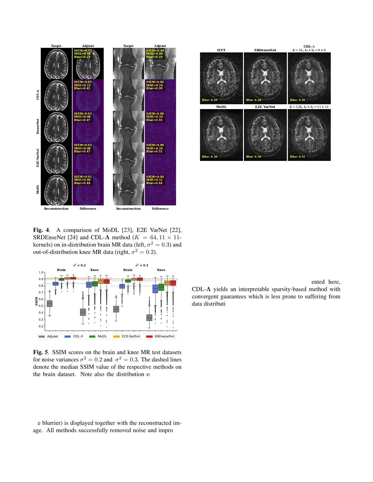
LEARNING SP A TIALL Y AD APTIVE SP ARSITY LEVEL MAPS FOR ARBITRAR Y CONV OLUTION AL DICTION ARIES J oshua Schulz ⋆ , David Schote ⋆ , Christoph K olbitsc h ⋆ , K ostas P apafitsor os † , Andr eas K ofler ⋆ ⋆ Physikalisch-T echnische Bundesanstalt (PTB), Braunschweig and Berlin, Germany † School of Mathematical Sciences, Queen Mary Uni versity of London, UK ABSTRA CT State-of-the-art learned reconstruction methods often rely on black-box modules that, despite their strong performance, raise questions about their interpretability and robustness. Here, we build on a recently proposed image reconstruction method, which is based on embedding data-driv en informa- tion into a model-based con volutional dictionary regulariza- tion via neural network-inferred spatially adapti ve sparsity lev el maps. By means of improved network design and ded- icated training strategies, we extend the method to achiev e filter-permutation inv ariance as well as the possibility to change the conv olutional dictionary at inference time. W e apply our method to low-field MRI and compare it to several other recent deep learning-based methods, also on in viv o data, in which the benefit for the use of a different dictionary is sho wcased. W e further assess the method’ s robustness when tested on in- and out-of-distribution data. When tested on the latter , the proposed method suffers less from the data distribution shift compared to the other learned methods, which we attribute to its reduced reliance on training data due to its underlying model-based reconstruction component. Index T erms — Neural Networks, Con v olutional Dictio- nary Learning, Sparsity , Adapti ve Regularization, Lo w-Field MRI 1. INTR ODUCTION Learned reconstruction methods using neural networks nowa- days, without a doubt, define the state-of-the-art in image re- construction [1]. Thereby , an important issue is their present black-box character . Often, one must seek a trade-of f be- tween empirical/numerical performance and interpretabil- ity/transparency , for example, in terms of the conv ergence guarantees of the derived reconstruction schemes [2]. Ad- ditionally , learned reconstruction methods are reported to quite consistently suffer from data-distribution shifts [3]. T o enhance interpretability , it is possible to carefully em- ploy learnable blocks such that the resulting reconstruction can be linked to a model-based variational problem, see e.g. [4], [5], [6], [7] and references therein. Dictionary-learning-based methods constitute another family of data-driv en reconstruction approaches [8] that are highly interpretable, yet so far few studies ha ve connected them to deep learning-based methods to improve their perfor- mance [9]. In [7], an image reconstruction method that lev erages spatially adapti ve sparsity of the image with respect to a pre-trained con volutional dictionary was introduced. The ov erall approach consists of an unrolled scheme that can be trained end-to-end, i.e. from the raw data measurements to the image estimate, where the sparsity le vel map is estimated by a conv olutional neural network (CNN) NET Θ . The main limitations in [7] lie in the architectural design of the NET Θ . The CNN is dictionary-agnostic, meaning that at inference time, it is not possible to use any other dictionary other than the one used for training. A change of the dictionary e.g. in terms of numbers of filters K - or even only in terms of their order - results in a loss of reconstruction performance. Here, we introduce a flexible frame work for learning spatially adaptiv e sparsity le vel maps that allows for the employment of arbitrary conv olutional dictionaries during inference. W e do so via a new CNN design customized to this task, training ov er different numbers of dictionaries and employing efficient dedicated training strategies. More specifically: (i) W e condition the CNN on the employed con volutional dictionary and adapt the architecture to achie ve dictio- nary filter permutation in v ariance and to allo w the use of dictionaries with a different number of filters. (ii) The con v olutional dictionaries are v aried during training, so that the network learns to estimate appropriate sparsity lev el maps for dif ferent dictionaries of arbitrary sizes. (iii) T runcated backpropagation is used during training, which is necessary since the considered reconstruction problem can be very lar ge due to the potential use of a lar ger num- ber of dictionary filters and larger CNN blocks. (iv) W e compare against other well-established methods using retrospecti vely simulated data, including out-of- distribution, showing that our approach is less af fected by the data distribution shift. Further, e xperiments on in viv o low-field MR data show that our approach, which benefits from using a dif ferent dictionary at inference, yields reconstructions that are on par with the other methods, while at the same time being interpretable. 2. METHODS W e briefly re vise the method in [7] to present the required concepts. Consider the typical in verse imaging problem y = Ax true + e , (1) where y denotes the raw measurement data obtained from the (unknown) image x true through the forward model A , and e denotes additiv e Gaussian noise. Since we focus on MR image reconstruction, here x true is complex-v alued. 2.1. Reconstruction with Spatially Adaptive Sparsity Level Maps Reconstructing an estimate of x true by solving (1) typically requires the use of re gularization methods. A successful reg- ularization mechanism can be designed based on spatially adaptiv e sparsity with respect to a pre-trained conv olutional dictionary D [8]. Here, one assumes that an image can be represented as a linear combination of sparse feature maps { s k } K k =1 that are conv olved with unit-norm conv olutional fil- ters { d k } K k =1 . For conciseness, we use the follo wing notation: s := [ s 1 , . . . , s K ] T , Ds := K X k =1 d k ∗ s k , B := AD . (2) As in [10], we also aim only to approximate the high-pass- filtered component of the image. Giv en x 0 := A H y , high- pass filtering of x 0 is achie ved by x high := x 0 − x low , where x low := argmin x 1 2 ∥ x − x 0 ∥ 2 2 + β 2 ∥∇ x ∥ 2 2 (PH) with β > 0 . W e strictly enforce the equality x high = Ds with sparse s and consider the reconstruction problem x ∗ := Ds ∗ + x low , (3) s ∗ := arg min s 1 2 ∥ Bs − y ′ ∥ 2 2 + ∥ Λ s ∥ 1 , (PR) where y ′ := y − Ax low and the sparsity lev el maps Λ := [ Λ 1 , . . . , Λ K ] T are parametrized as outputs of a deep CNN NET Θ with parameters Θ applied to some input. The method [7] (named CDL- Λ ; Con v olutional Dictionary Learning with Λ -maps), performs the learned high-pass filtering by solving problem (PH), the estimation of the sparsity level maps Λ , and the final reconstruction of the image by solving (PR) by means of algorithm unrolling [11] of an accelerated proximal gradient descent (FIST A) [12] with conv ergence guarantees [13]. W e denote the entire reconstruction network by N T Θ (see Figure 1) and the FIST A-scheme to approximately solve (PR) with T ∈ N iterations s T := FIST A T ( s 0 , A , D , y ′ , Λ ) with starting value s 0 = 0 ∈ C N K . 2.2. Dictionary-Agnostic vs Dictionary-A ware Learning of the Sparsity Level Maps W e in vestigate three dif ferent possibilities to construct the network NET Θ for estimating spatially adaptiv e sparsity lev el maps Λ , see Figure 1 (bottom) for an ov erview . Complex- valued images x ∈ C N are treated as real-valued two-channel images, and we use real-valued dictionary filters, i.e., Ds = K X k =1 d k ∗ s k := K X k =1  d k ∗ Re( s k ) + i d k ∗ Im( s k )  , implying that for any s ∈ C N K , and z = [ z 1 , z 2 ] T ∈ C N Ds = [ D , D ][Re( s ) , Im( s )] T , D T z := [ D T z 1 , D T z 2 ] T . The weighted ℓ 1 -norm in (PR) is then defined by ∥ s ∥ 1 :=   [Re( s ) , Im( s )] T   1 . In [7], NET Θ was constructed as a U- Net that estimates K sparsity lev el maps Λ := [ Λ 1 , . . . , Λ K ] (shared between real and imaginary parts of s ) from the input image, i.e., upon vectorization of 2D images to v ectors, it holds Λ = NET Θ ( x 0 ) with Λ k :=  NET Θ ( x 0 )  k := t · ϕ ◦ ( u Θ ( x 0 )) k , (V1) with global learnable scalar parameter t > 0 , Softplus acti- vation function ϕ and a 2-to- K 2D U-Net u Θ . While proven effecti v e, it is evident from (V1) that the network is agnostic with respect to the dictionary D as well as only applicable to dictionaries with a fixed number of filters K . W e refer to the CNN architecture in (V1) as ” NET Θ V1”. A straight forward solution to condition the network NET Θ on the dictionary D is to provide a dictionary-dependent input and use a K -to- K 2D U-Net u Θ to obtain Λ := NET Θ ( D T x 0 ) := t · ϕ ◦ u Θ ( D T x 0 ) , (V2) which we refer to as ” NET Θ V2”. Although using a dictionary- dependent input, NET Θ V2 is nevertheless inherently linked to the number of filters K . Thus, we consider the third variant ” NET Θ V3”, which, by slight abuse of notation, reads as Λ := NET Θ ( D T x 0 ) := R − 1 t · ϕ ◦ u Θ ( RD T x 0 ) , (V3) where R and R − 1 are operators that reshape the input tensors by moving the channel’ s dimension to the batch-dimension, i.e., the y transform inputs with shapes (batc h , 2 · K, N y , N x ) to (batc h · K , 2 , N y , N x ) and from (batc h · K , 1 , N y , N x ) to (batc h , K, N y , N x ) , respectively . Here, u Θ denotes a 2-to- 1 2D U-Net. In contrast to V1 and V2, the same 2D U-Net is employed to estimate the corresponding sparsity lev el map Λ k ∈ R N > 0 from the input ( D T x 0 ) k ∈ R 2 N . By doing so, NET Θ can be employed with dictionaries with an arbitrary number of filters K at inference. 2.3. Network T raining Instead of a single, fixed dictionary , here, we employ an entire set of conv olutional dictionaries D with different numbers of Unr olled A cceler at ed Pr o ximal Gr adient Algorithm Sol v e (PH) Sol v e (PR) Sparsity Le v el Map Estimation -Maps Estimation Ar chit ectur es Learned Hig h-P ass Filt ering Measur ed Data V ersion 1 V ersion 2 R eshape R eshape V ersion 3 Input Image Estimat e Fig. 1 . The reconstruction pipeline of the CDL- Λ method and the three different versions of NET Θ (V1 – V3) (orange blocks) in vestigated in this study . First, a learned high-pass filtering step solving (PH) is performed (gr een block) . Then, NET Θ estimates spatially varying sparsity lev el maps from an input (blue block) . Last, a FIST A algorithm is unrolled to obtain an approximate solution of (PR) (ocher block) . An estimate of the solution is obtained by adding the low-frequency component that was extracted in the first block. In contrast to V1 and V2, the proposed improved V3 is permutation in variant and allo ws for the use of dictionaries with a different number of filters K . filters K and kernel sizes k f × k f . Giv en training data, we minimize a mean squared error (MSE)-based loss function L (Θ) := X y , x true , D MSE  N T Θ ( y , D ) , x true  , (4) which means that the network NET Θ is exposed not only to various ra w data-target pairs, but also to different reconstruc- tion problems of the form (PR). Being able to employ larger dictionaries in terms of larger K and kernel size k f × k f with richer structure implies increased memory consumption when unrolling the FIST A- block. Therefore, employing truncated back-propagation [14] is an attractiv e choice for unrolling a relati vely large number of iterations with many large intermediate quan- tities. More precisely , during training, we first compute s T ′ = FIST A T ′ ( s 0 , A , D , y ′ , Λ ) with the FIST A-block with the current estimate of Λ without tracking gradients. Then, we perform additional T − T ′ unrolled iterations (starting the FIST A iteration from s T ′ ) by also tracking the gradients of Θ to train by minimizing (4). W e used T = 64 and T ′ = 36 . 2.4. Datasets and Evaluation Metrics Here, we conduct experiments on a lo w-field (LF) MR re- construction problem. LF MRI suffers from high noise and low image resolution due to hardware constraints. W e there- fore model the forw ard operator A in (1) by A := S I F , where F denotes a 2D Fourier transform and S I a binary mask that masks out the outer region of the measurements y , modeling the low-resolution acquisition. W e used brain MR (4875/1393/696 images for training/validation/testing) and 3951 knee MR images from the fastMRI dataset [15] to retrospectively simulate data according to (1). The v ari- ance of the noise component e in (1) is set relativ ely high by σ 2 ∈ { 0 . 2 , 0 . 3 } . Further , we show an application of the methods to an in vi vo T2-weighted brain image acquired with the Open Source Imaging Initiati ve (OSI 2 ) LF MR scan- ner [16]. For ev aluation, we report the MSE, the structural similarity index measure (SSIM), as well as the reference- free blur image metric [17], which is especially informati ve for the in vi vo data, where no target image exists. T o fo- cus on the diagnostic content, all metrics are computed by discarding the background of the images, emplo ying masks deriv ed from the target images. The MSE and SSIM were calculated using the MRpro library [18], which allo ws for the definition of such masks, while the blur metric implementa- tion is from Scikit-learn [19]. For MoDL, E2E V arNet, SRDenseNet, and CDL- Λ , we used a learning rate of 10 − 4 for the employed CNN-blocks, and 10 − 2 for the learned step sizes/scalars. CDL- Λ was trained for 48 epochs using a batch size of 1, the others for 128 epochs using a batch size of 4. Code and further training details are av ailable at here. 2.5. Pre-T raining the Dictionaries W e pre-trained different conv olutional dictionaries with dif- ferent numbers of filters K of kernel sizes k f × k f . For doing that, we employed the sparse coding library SPORCO [20] to solve a conv olutional dictionary learning problem us- ing 360 brain MR images using the online dictionary learn- ing method described in [21] for different choices of β = 0 . 1 , 0 . 25 , 0 . 5 in (PH), scalar sparsity le vel parameters λ = 0 . 1 , 0 . 5 , 2 , 4 , kernel sizes k f = 9 , 11 and number of filters K = 16 , 32 , 64 , 128 , resulting in an overall number of 96 different dictionaries. Note that we do not use the K = 128 - dictionaries when minimizing (4) due to GPU-memory con- straints. 2.6. Methods of Comparison W e compare against the End-to-End V ariational Network (E2E V arNet) [22], the model-based deep learning (MoDL) [23], and a low-field MRI super-resolution (SR) approach, SRDenseNet [24]. The first two methods both employ the measured data y , while the latter maps the IFFT recon- struction obtained from the 160 × 160 k -space data to a V1 V2 V3 Base SSIM 0 . 85 ± 0 . 05 0 . 83 ± 0 . 05 0 . 82 ± 0 . 05 MSE 0 . 11 ± 0 . 04 0 . 14 ± 0 . 06 0 . 14 ± 0 . 06 π 1 ∆ SSIM − 0 . 06 ± 0 . 01 − 0 . 08 ± 0 . 03 0 ∆ MSE 0 . 12 ± 0 . 04 0 . 14 ± 0 . 10 0 π 2 ∆ SSIM − 0 . 05 ± 0 . 01 − 0 . 05 ± 0 . 02 0 ∆ MSE 0 . 12 ± 0 . 04 0 . 12 ± 0 . 08 0 π 3 ∆ SSIM − 0 . 05 ± 0 . 01 − 0 . 08 ± 0 . 03 0 ∆ MSE 0 . 11 ± 0 . 04 0 . 17 ± 0 . 11 0 T able 1 . Results for NET Θ as in (V1), (V2) and (V3) for three filter permutations π 1 , π 2 , π 3 , shown for K = 32 , 11 × 11 -kernels. The improved V3 is filter permutation in v ariant by construction. Note that differences between the baselines of V1, V2, and V3 can be attributed to the de viations of the three v ersions in terms of the number of trainable parameters, which can be easily addressed by increasing them. 320 × 320 -sized image. Our implementations of MoDL, E2E V arNet and SRDenseNet contain 113 413 , 34 512 846 and 5 654 834 trainable parameters. MoDL is unrolled for T = 10 iterations and alternates between the application of the CNN-block and a data-consistenc y (DC) step inv olving a learnable scalar parameter λ > 0 that is shared among the iterations. E2E V arNet is unrolled with T = 12 iter- ations and contains iteration-dependent learned step-sizes. MoDL and E2E V arNet were accordingly adapted to the here considered single-coil case, i.e., the DC step in MoDL has a closed-form solution instead of requiring a conjugate gradient method, and E2E V arNet does not employ a coil-sensitivity map-refinement module. CDL- Λ contains 8 266 914 and 2 104 802 trainable parameters for V1 and V2, respectively , while for V3, we use a more shallow U-Net with only 112 067 trainable parameters (dictionary filters not included). 3. RESUL TS Dictionary F ilter-P ermutation In variance and Dif fer ent Num- bers of F ilters K : T able 1 sho ws the change in SSIM and MSE when the three different versions of NET Θ described in (V1), (V2), and (V3) are exposed to a permutation of the dictionary filters. In this case, training was carried out using only one dictionary D with K = 32 filters of size k f × k f = 11 × 11 . As sho wn, all three versions achieve approximately the same performance in terms of SSIM and MSE, while V3 is the only one to remain in variant under filter order permu- tation. Additionally , when training the improved NET Θ V3 according to (4), it is now possible to employ a different dic- tionary D at inference by maintaining a comparable perfor- mance, see Figure 2. Inspection of the Sparsity Le vel Maps: Figure 3 shows an ex emplary comparison of eight Λ -maps for NET Θ (V1)-(V3) for a dictionary with K = 32 filters of size k f × k f = 11 × 11 . k f = 1 1 , = 0 . 1 , = 0 . 2 5 k f = 1 1 , = 0 . 5 , = 0 . 5 k f = 9 , = 0 . 1 , = 0 . 2 5 k f = 9 , = 0 . 5 , = 0 . 5 0.00 0.05 0.10 0.15 0.20 0.25 0.30 0.35 MSE K = 1 6 k f = 1 1 , = 0 . 1 , = 0 . 2 5 k f = 1 1 , = 0 . 5 , = 0 . 5 k f = 9 , = 0 . 1 , = 0 . 2 5 k f = 9 , = 0 . 5 , = 0 . 5 K = 3 2 k f = 1 1 , = 0 . 1 , = 0 . 2 5 k f = 1 1 , = 0 . 5 , = 0 . 5 k f = 9 , = 0 . 1 , = 0 . 2 5 k f = 9 , = 0 . 5 , = 0 . 5 K = 6 4 k f = 1 1 , = 0 . 1 , = 0 . 2 5 k f = 1 1 , = 0 . 5 , = 0 . 5 k f = 9 , = 0 . 1 , = 0 . 2 5 k f = 9 , = 0 . 5 , = 0 . 5 K = 1 2 8 Fig. 2 . MSE obtained by CDL- Λ with NET Θ V3 over the brain MR test set for 16 different choices of dictionaries. Note that, for training, we did not use the K = 128 -dictionaries. V ersion 1 Ch 18 Ch 20 Ch 25 Ch 12 Ch 17 Ch 27 Ch 11 Ch 6 V ersion 2 Ch 12 Ch 6 Ch 24 Ch 25 Ch 11 Ch 2 Ch 20 Ch 27 V ersion 3 Ch 5 Ch 12 Ch 27 Ch 8 Ch 11 Ch 20 Ch 16 Ch 29 Fig. 3 . Eight out of K = 32 Λ -maps with the largest v ari- ance, seen as indicati ve of the filter’ s importance in the image representation, for each NET Θ V1, V2, V3, and for filter size k f × k f = 11 × 11 . The shown maps are those with the largest variances relative to the entire set of Λ -maps for each version. The figure con- firms that all three versions of NET Θ assign similar impor- tance (indicated by the lar ger variance of the corresponding map, see also [7]) to the respective filter . For example, fil- ter 25 in V1 appears to contribute to the representation of the image also in V2, filter 12 and 20 in all three versions, etc. Comparison to Other Methods: Figure 4 sho ws a visual comparison of the adjoint reconstruction, MoDL, E2E V ar- Net, SRDenseNet, and the inv estigated CDL- Λ using K = 64 filters of size k f × k f = 11 × 11 for a brain and knee MR image, together with their respective error images and image metrics. Despite yielding accurate reconstructions, CDL- Λ is surpassed by all other learned methods. Ho we ver , when tested on out-of-distrib ution data, i.e., on the knee images, the performance gap between the different methods is noticeably reduced. For example, compare the reduced difference be- tween MoDL and CDL- Λ in terms of SSIM for brain vs knee images, for σ 2 = 0 . 2 and σ 2 = 0 . 3 in Figure 5. Application to In V ivo Data: Figure 6 shows a compari- son of the methods applied to a T2-weighted in vi vo image. T arget S SIM=0.53 MSE=0.44 Blur=0.23 Adjoint CDL- S SIM=0.85 MSE=0.13 Blur=0.41 DenseNet S SIM=0.93 MSE=0.08 Blur=0.47 E2E - V arNet S SIM=0.93 MSE=0.08 Blur=0.47 MoDL Reconstruction S SIM=0.91 MSE=0.09 Blur=0.44 Difference T arget S SIM=0.44 MSE=0.66 Blur=0.19 Adjoint S SIM=0.82 MSE=0.14 Blur=0.39 S SIM=0.86 MSE=0.10 Blur=0.55 S SIM=0.86 MSE=0.10 Blur=0.51 Reconstruction S SIM=0.84 MSE=0.11 Blur=0.44 Difference Fig. 4 . A comparison of MoDL [23], E2E V arNet [22], SRDEnseNet [24] and CDL- Λ method ( K = 64 , 11 × 11 - kernels) on in-distribution brain MR data (left, σ 2 = 0 . 3 ) and out-of-distribution knee MR data (right, σ 2 = 0 . 2 ). 0.2 0.3 0.4 0.5 0.6 0.7 0.8 0.9 1.0 S SIM Brain Knee Brain Knee 2 = 0 . 2 2 = 0 . 3 Adjoint C D L - MoDL E2E - V arNet SRDenseNet Fig. 5 . SSIM scores on the brain and knee MR test datasets for noise variances σ 2 = 0 . 2 and σ 2 = 0 . 3 . The dashed lines denote the median SSIM value of the respectiv e methods on the brain dataset. Note also the distribution of outliers for the knee test set, where, in some rare cases, E2E V arNet and SRDenseNet e ven seem to deteriorate the images compared to the adjoint. Since no target image is av ailable, the blur metric (the higher , the blurrier) is displayed together with the reconstructed im- age. All methods successfully removed noise and improved the resolution, producing comparable results, with MoDL Blur: 0.20 IFFT Blur: 0.28 SRDenseNet Blur: 0.36 C D L - K = 1 6 , k f × k f = 9 × 9 Blur: 0.36 MoDL Blur: 0.30 E2E V arNet Blur: 0.31 K = 1 2 8 , k f × k f = 1 1 × 1 1 Fig. 6 . In vivo T2-weighted brain MR image: MoDL, E2E V arNet and SRDenseNet, and the CDL- Λ with the improved NET Θ (V3), once with K = 16 filters of size k f × k f = 9 × 9 , and once with K = 128 , k f × k f = 11 × 11 . Note how the use of a larger dictionary at inference, which was not used in training, leads to a sharper result. exhibiting a slight tendency to oversmooth image details. Observe also ho w CDL- Λ in this case benefits from using a larger dictionary at inference ( K = 128 ) that leads to a sharper result. 4. CONCLUSION T ogether with the improved CNN-block presented here, CDL- Λ yields an interpretable sparsity-based method with con ver gent guarantees which is less prone to suffering from data distribution shifts compared to MoDL, E2E V arNet and SRDenseNet. This can be explained by the reduced reliance on training data due to its underlying model-based reconstruc- tion component. Indeed, the CNN-block NET Θ in CDL- Λ , solely estimates the Λ -maps, and the re gularizational effect comes from the sparsity imposed in (PR), whereas in the other approaches, deep CNNs are directly responsible for the reduction of noise and artefacts. Furthermore, with the improved CNN-block NET Θ V3, CDL- Λ can no w be equipped with a general sparsity le vel map estimator for arbitrary con volutional dictionaries. W e showed that thanks to the use of a larger dictionary at infer- ence, competiti ve performance can be achie ved for in vi vo data as well. Our work pav es the way to be able to utilize the estimated sparsity le vel maps to further adapt the dictio- nary filters as well as to de velop rejection and/or replacement strategies for less useful dictionary filters for the image rep- resentation, possibly in a zero-shot self-supervised fashion. 5. REFERENCES [1] S. Arridge, P . Maass, O. ¨ Oktem, and C.-B. Sch ¨ onlieb, “Solving in verse problems using data-dri ven models, ” Acta Numer . , vol. 28, pp. 1–174, 2019. [2] S. Mukherjee, A. Hauptmann, O. ¨ Oktem, M. Pere yra, and C. B. Sch ¨ onlieb, “Learned reconstruction methods with con ver gence guarantees: A survey of concepts and applications, ” IEEE Signal Process. Mag. , vol. 40, no. 1, pp. 164–182, 2023. [3] M. Z. Darestani, A. S. Chaudhari, and R. Heckel, “Mea- suring robustness in deep learning based compressi ve sensing, ” in ICML , 2021, pp. 2433–2444. [4] H. Li, J. Schwab, S. Antholzer, and M. Haltmeier , “NETT: solving inv erse problems with deep neural net- works, ” Inver se Pr obl. , vol. 36, no. 6, pp. 065005, 2020. [5] E. Kobler , A. Effland, K. K unisch, and T . Pock, “T o- tal deep v ariation: A stable regularization method for in verse problems, ” IEEE TP AMI , vol. 44, no. 12, pp. 9163–9180, 2021. [6] M. Pourya, E. K obler , M. Unser , and S. Neumayer , “DEALing with image reconstruction: Deep attenti ve least squares, ” in ICML , 2025. [7] A. K ofler , L. Calatroni, C. Kolbitsch, and K. Papafit- soros, “Learning spatially adapti ve ℓ 1 -norms weights for con v olutional synthesis regularization, ” in 33r d EU- SIPCO , 2025, pp. 1782–1786. [8] C. Garcia-Cardona and B. W ohlberg, “Conv olutional dictionary learning: A comparativ e revie w and new al- gorithms, ” IEEE T r ans. Comput. Ima g. , vol. 4, no. 3, pp. 366–381, 2018. [9] M. Scetbon, M. Elad, and P . Milanfar , “Deep K-SVD denoising, ” IEEE T r ans. Ima ge Pr ocess. , v ol. 30, pp. 5944–5955, 2021. [10] B. W ohlberg, “Con volutional sparse representations as an image model for impulse noise restoration, ” in IEEE 12th IVMSP workshop , 2016, pp. 1–5. [11] V . Monga, Y . Li, and Y . C. Eldar , “ Algorithm unrolling: Interpretable, efficient deep learning for signal and im- age processing, ” IEEE Signal Pr ocess. Mag . , vol. 38, no. 2, pp. 18–44, 2021. [12] A. Beck and M. T eboulle, “ A fast iterativ e shrinkage- thresholding algorithm for linear inv erse problems, ” SIAM J. Ima ging Sci. , vol. 2, no. 1, pp. 183–202, 2009. [13] A. Chambolle and C. H. Dossal, “On the con ver gence of the iterates of ”FIST A”, ” J. Optim. Theory Appl. , vol. 166, no. 3, pp. 25, 2015. [14] A. Shaban, A. A. Cheng, N. Hatch, and B. Boots, “Trun- cated back-propagation for bile vel optimization, ” in 22nd AIST A TS , 2019, pp. 1723–1732. [15] J. Zbontar , F . Knoll, A. Sriram, T . Murrell, Z. Huang, M. J. Muckley , A. Def azio, R. Stern, P . Johnson, M. Bruno, M. Parente, K. J. Geras, J. Katsnelson, H. Chandarana, Z. Zhang, M. Drozdzal, A. Romero, M. Rabbat, P . V incent, N. Y akubov a, J. Pinkerton, D. W ang, E. Owens, C. L. Zitnick, M. P . Recht, D. K. Sodickson, and Y . W . Lui, “fastMRI: An open dataset and benchmarks for accelerated MRI, ” 2018. [16] L. W inter , “OSI 2 community . OSI 2 ONE MR scanner . open source imaging, ” https://www .opensourceimaging.org /project/osii-one/. [17] F . Crete, T . Dolmiere, P . Ladret, and M. Nicolas, “The blur ef fect: perception and estimation with a ne w no- reference perceptual blur metric, ” in HVEI XII . SPIE, 2007, vol. 6492, pp. 196–206. [18] F . F . Zimmermann, P . Schuenke, S. Brahma, M. Guas- tini, J. Hammacher, A. K ofler , C. Kranich Redshaw , L. Lunin, S. Martin, D. Schote, and C. K olbitsch, “MR- pro - PyT orch-based MR image reconstruction and pro- cessing package, ” Feb. 2025. [19] Oliv er Kramer, “Scikit-learn, ” in Machine learning for evolution str ate gies , pp. 45–53. Springer , 2016. [20] B. W ohlberg, “SPORCO: A python package for stan- dard and conv olutional sparse representations, ” in SciPy , 2017, pp. 1–8. [21] J. Liu, C. Garcia-Cardona, B. W ohlberg, and W . Y in, “First-and second-order methods for online conv olu- tional dictionary learning, ” SIAM J. Imaging Sci. , v ol. 11, no. 2, pp. 1589–1628, 2018. [22] A. Sriram, J. Zbontar , T . Murrell, A. Defazio, C. L. Zit- nick, N. Y akubov a, F . Knoll, and P . Johnson, “End- to-end variational networks for accelerated MRI recon- struction, ” in MICCAI . Springer , 2020, pp. 64–73. [23] H. K. Aggarwal, M. P . Mani, and M Jacob, “MoDL: Model-based deep learning architecture for in v erse problems, ” IEEE T r ans. Med. Imaging , vol. 38, no. 2, pp. 394–405, 2018. [24] M. L. de Leeuw Den Bouter , G. Ippolito, T . P . A. O’Reilly , R. F . Remis, M. B. V an Gijzen, and A. G. W ebb, “Deep learning-based single image super- resolution for low-field MR brain images, ” Sci. Rep. , vol. 12, no. 1, pp. 6362, 2022.