Learning Complex Physical Regimes via Coverage-oriented Uncertainty Quantification: An application to the Critical Heat Flux

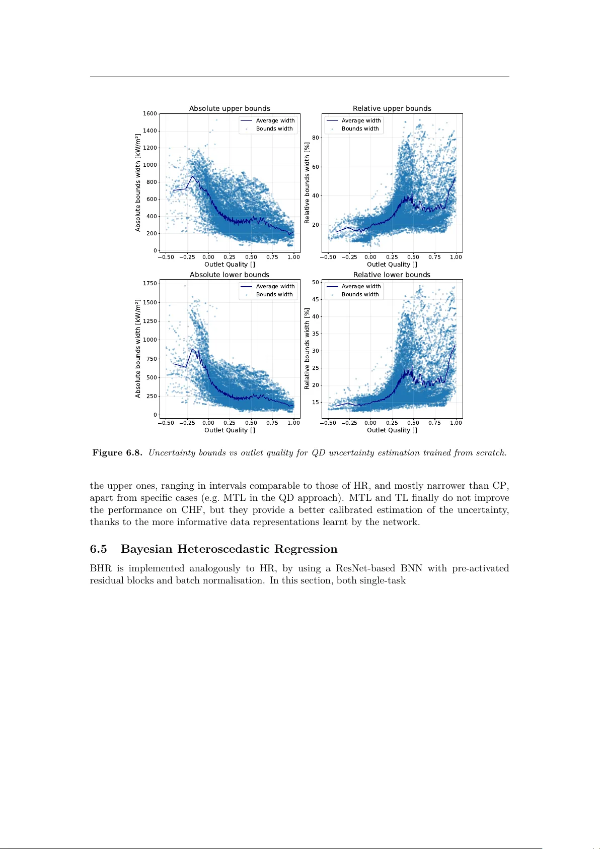
Learning Complex Ph ysical Regimes via Co v erage-orien ted Uncertain t y Quan tiﬁcation An application to the Critical Heat Flux Mic hele Cazzola ∗ 1 , Alberto Ghione † 1 , Lucia Sargen tini ‡ 1 , Julien Nesp oulous § 2 and Riccardo Finotello ¶ 2 1 Univ ersité P aris Sacla y , Cea , Service Thermo-hydraulique et Mécanique des Fluides ( Stmf ), Gif-sur-Y v ette, F-91191, F rance 2 Univ ersité P aris Sacla y , Cea , Service de Génie Logiciel p our la Simulation ( Sgls ), Gif-sur-Y v ette, F-91191, F rance Abstract A central challenge in scien tiﬁc machine learning (ML) is the correct represen tation of ph ysical systems go v erned b y complex, m ulti-regime behaviours. In these scenarios, standard data analysis tec hniques often fail to capture the changing nature of the data, as the system’s resp o nse v aries signiﬁcantly across the state space due to the inherent stochasticit y and the diﬀerent physical regimes. Uncertain ty quantiﬁcation (UQ) should thus not be viewed merely as a safet y assessmen t, but as a fundamental supp ort to the learning task itself, guiding the mo del to internalise the underlying b eha viour of the data. W e address this c hallenge by focusing on the Critic al He at Flux (CHF) benchmark and dataset presented b y the OECD/NEA Exp ert Gr oup on R e actor Systems Multi-Physics . This case study represen ts a rigorous test for scien tiﬁc ML due to the highly non-linear dep endence of CHF on the inputs and the existence of distinct microscopic physical regimes. These regimes exhibit diverse statistical proﬁles, a complexity that requires adv anced UQ tec hniques to in ternalise the underlying data behaviour and ensure reliable predictions. In this w ork, we conduct a comparativ e analysis of UQ methodologies to determine their impact on physical representation. W e contrast post-ho c metho ds, sp eciﬁcally conformal prediction, against end-to-end co verage-orien ted pipelines, including (Ba yesian) heterosce- dastic regression and qualit y-driv en loss functions. These end-to-end approaches treat un- certain ty not as a ﬁnal metric, but as an active comp onen t of the optimisation process, mo delling the prediction and its statistical behaviour simultaneously . W e show that while post-ho c metho ds ensure rigorous statistical calibration, co verage- orien ted learning eﬀectively reshap es the mo del’s representation to match the complex phys- ical regimes. The result is a model that delivers not only high predictive accuracy but also a physically consisten t uncertain ty estimation that adapts dynamically to the intrinsic v ari- abilit y of the CHF phenomenon. k eywords: uncertain ty quantiﬁcation, representation learning, mac hine learning, scien tiﬁc mac hine learning, critical heat ﬂux highligh ts: W e sho w that uncertain ty quan tiﬁcation can b e used actively during the learning phase to mo del complex physical regimes. W e consider the computation of the critical heat ﬂux as a use case, and w e show that co verage-orien ted uncertain ty quan tiﬁcation can be used to make the model more accurate and reliable. ∗ e-mail: michele.cazzola@cea.fr † e-mail: alberto.ghione@cea.fr ‡ e-mail: lucia.sargentini@cea.fr § e-mail: julien.nespoulous@cea.fr ¶ e-mail: riccardo.finotello@cea.fr 1 CONTENTS Con ten ts 1 In tro duction 3 2 Related W ork 4 3 The U.S. Nuclear Regulatory Commission Dataset 6 4 Metho dology 8 4.1 Residual Netw orks for Ph ysics Surrogate Mo dels . . . . . . . . . . . . . . . . . . 8 4.2 Loss F unctions and Optimisation . . . . . . . . . . . . . . . . . . . . . . . . . . . 9 4.3 Uncertain ty Quan tiﬁcation T echniques . . . . . . . . . . . . . . . . . . . . . . . . 9 4.4 Heteroscedasticit y tests . . . . . . . . . . . . . . . . . . . . . . . . . . . . . . . . 10 4.5 Conformal Prediction . . . . . . . . . . . . . . . . . . . . . . . . . . . . . . . . . 11 4.6 Heteroscedastic Regression . . . . . . . . . . . . . . . . . . . . . . . . . . . . . . . 13 4.7 Qualit y-Driven Prediction and Uncertain ty Estimation . . . . . . . . . . . . . . . 14 4.8 Ba yesian Heteroscedastic Regression . . . . . . . . . . . . . . . . . . . . . . . . . 16 5 Ev aluation metrics 17 5.1 Mac hine Learning Metrics . . . . . . . . . . . . . . . . . . . . . . . . . . . . . . . 17 5.2 Uncertain ty Quan tiﬁcation Metrics . . . . . . . . . . . . . . . . . . . . . . . . . . 18 6 Results 20 6.1 Residual Netw orks . . . . . . . . . . . . . . . . . . . . . . . . . . . . . . . . . . . 20 6.2 Conformal Prediction . . . . . . . . . . . . . . . . . . . . . . . . . . . . . . . . . 21 6.3 Heteroscedastic Regression . . . . . . . . . . . . . . . . . . . . . . . . . . . . . . . 24 6.4 Qualit y-Driven Prediction and Uncertain ty Estimation . . . . . . . . . . . . . . . 27 6.5 Ba yesian Heteroscedastic Regression . . . . . . . . . . . . . . . . . . . . . . . . . 30 7 Conclusion 33 2 1 INTRODUCTION 1 In tro duction Mac hine learning (ML) has deeply reshap ed the wa y scientiﬁc data is analysed, providing p o w er- ful and ﬂexible tools to mo del complex dep endencies hidden in large and high-dimensional exp er- imen tal datasets. Unlike traditional empirical correlations and phenomenological models, often constrained by rigid or ov erly simplistic functional forms, data-driv en approaches can adapt- iv ely mo del the complex b eha viours typical of ph ysical phenomena. This ﬂexibility has driv en their widespread adoption across scientiﬁc domains, from particle physics to nuclear engineering, where they serve not only as surrogates but also as tools for hypothesis generation and exp eri- men tal design. Ho wev er, the known black-box nature of many ML metho ds has raised concerns ab out their reliabilit y and interpretabilit y , esp ecially as they transition from auxiliary to ols to core comp onen ts of scientiﬁc workﬂo ws. Scien tiﬁc ML is increasingly tasked with constructing surrogate mo dels that do not merely inter- p olate exp erimen tal data, but capture the underlying ph ysical la ws and statistical b eha viours of the system [ 1 ]. While standard ML regression approaches prioritise the minimisation of a global error metric, suc h as the mean squared error, this ob jectiv e can b e insuﬃcien t for ph ysical applic- ations c haracterised b y complex, multi-regime dynamics. In these scenarios, the observed data often exhibits v arying degrees of sto c hasticity dep end ing on the region of the input state space. Consequen tly , a reductive approach that aims solely to minimise prediction interv als risks mask- ing the intrinsic v ariability of the phenomenon. By treating natural ﬂuctuations as noise to be suppressed, a mo del may ac hieve high nominal precision but fails to learn a correct representation of the ph ysical reality , leading to o v erconﬁdent predictions in turbulen t or unstable regimes [ 2 ]. Therefore, a robust scientiﬁc mo del must internalise this v ariabilit y , treating the uncertaint y not as a residual error, but as a fundamen tal comp onen t of the physical representation. In this framework, uncertain ty quantiﬁc ation (UQ) serves as a critical to ol for assessing the trust worthiness and physical consistency of the learned representation [ 1 ]. Rather than b eing a mere post-pro cessing step for safet y compliance, UQ pro vides a quan titative measure of how w ell the mo del’s conﬁdence aligns with the observ ed data distribution and a wa y to include this uncertain ty directly in to the learning pro cess. A rigorous criterion for this assessment is statistical co verage, deﬁned as the probability that the true v alue of a physical quantit y falls within the predicted uncertain ty b ounds. Ensuring consistent cov erage across the entire input domain is essen tial for establishing trust in the mo del, particularly in high-stak es scientiﬁc applications. F rom a ph ysical persp ectiv e, cov erage-based metho ds allow the model to reveal changes in system b eha viour: a localised expansion of uncertaint y b ounds is often a direct signature of a transition to a diﬀeren t regime, more sto c hastic or out-of-distribution with resp ect to the training data, where the mo del loses conﬁdence in its o wn predictions. One possible example of these changes ma y b e the onset of physical instabilities or phase transitions. Thus, achieving correct cov erage is not just a statistical requiremen t but a means to v alidate that the mo del has correctly identiﬁed and internalised the distinct physical regimes presen t in the data. W e argue that ac hieving this rigorous cov erage can be approached in tw o distinct wa ys, with diﬀeren t impacts on the mo del’s representation pow er. The ﬁrst is a p ost-ho c approac h, such as conformal prediction (CP) [ 3 ], which calibrates the uncertain ty of a frozen, pre-trained mo del. While in v aluable for establishing statistical guarantees and “trust w orthiness” on existing blac k b o xes, this metho d does not alter the mo del’s in ternal understanding of the ph ysics. It treats the mo del as a static en tity , applying corrections to its outputs without inﬂuencing its learned features or representations. Thus, the model remains oblivious to the underlying m ulti-regime nature of the data, though the uncertain ty b ounds are an attempt to reﬂect changes in the data b eha viour and mo del trust worthiness. The second, and more transformative approac h, is to actively learn 3 2 RELA TED WORK the uncertain ty during training. By integrating cov erage-oriented ob jectiv es directly into the loss function, for instance through qualit y-driven techniques (QD) [ 4 ] or (Ba yesian) heteroscedastic regression (HR) [ 5 ], we can force the mo del to ackno wledge and adapt to the heteroscedastic nature of the data. This activ e learning process do es more than just quantify error; it improv es the representation pow er of the mo del, allo wing it to adapt its internal features to the c hanges in the b eha viour of the system across the input space [ 6 ], eﬀectiv ely “learning” the phase changes of the physics for the downstream task. W e test these hypotheses on the prediction of the Critic al He at Flux (CHF), a phenomenon that serv es as a rigorous b enc hmark for multi-regime scientiﬁc ML. CHF is characterised by a highly non-linear dep endence on its inputs and arises from distinct microscopic mechanisms, dep artur e fr om nucle ate b oiling (DNB) and dryout , which exhibit v astly diﬀerent statistical proﬁles [ 7 , 8 ]. Recognising this complexity , the OECD/NEA Exp ert Gr oup on R e actor Systems Multi-Physics established a b enc hmark to develop ML strategies capable of na vigating these regimes [ 9 ]. In the sp eciﬁc context of nuclear safet y , the alignment b et w een predicted uncertaint y and empirical v ariability is formalised in the Best Estimate plus Unc ertainty (BEPU) metho dology [ 10 , 11 ]. Using this challenging dataset [ 12 ], we demonstrate that while CP acts as a p ost-hoc implemen t- ation of the BEPU framew ork ensuring safet y , cov erage-orien ted learning yields mo dels that are ph ysically consistent and robust b y design, oﬀering a represen tation-enhanced approach to the same rigorous safet y standards. This article also represen ts the ﬁrst case study of the applica- tion of QD loss to the CHF regression problem, showing how this metho d can b e used to achiev e co verage-based learning and to improv e the physical representation of the model. The article is organised as follows: • Section 2 brieﬂy recalls the main research w orks conducted on ML and UQ for the prediction of the CHF in thermal hydraulics; • Section 3 details the charac teristics of the OECD/NEA b enc hmark dataset and the pre- pro cessing required to exp ose its physical structure; • Section 4 establishes a theoretical o verview of the ML and UQ tec hniques used in the article. This includes our prop osal of an approach based on cov erage and quality-driv en metho ds to correctly assess the uncertain ties for any given mo del; • Section 5 deﬁnes the ev aluation metrics used to assess b oth predictive p erformance and uncertain ty calibration; • Section 6 presen ts the comparative analysis, ev aluating b oth predictive performance and ph ysical consistency; • Section 7 summarises the impact of cov erage-based learning on scientiﬁc representation. 2 Related W ork T raditionally , the prediction of CHF has relied on phenomenological approaches, which are often constrained to sp eciﬁc operating conditions. Early to ols were mo dels based on empirical correl- ations and simpliﬁed analytical models that captured certain asp ects of the underlying physics, with each mo del having its own limited v alidity range. F or instance, some of the pioneering cor- relations for CHF prediction, such as the Biasi c orr elation [ 13 ], were based on empirical mo dels with minimal v alidit y domains. These were succeeded by more comprehensiv e lo ok-up tables (LUT), such as the 2006 Gr o eneveld LUT [ 14 ], whic h ﬁt p olynomial functions to larger data- bases. While these methods expanded the domain of application and are still widely used in CHF 4 2 RELA TED WORK regression, they remain static representations that struggle to capture the complex, m ulti-regime nature of the phenomenon: on the b enc hmark dataset (see Section 3 ), they reach 66% (Biasi) and 36% (Gro enev eld LUT) of ro ot mean squared percentage error (RMSPE, see ( 5.3 ) for the deﬁnition). The inheren t limitations of these ﬁxed correlations motiv ated the exploration of data-driv en strategies. Early ML works inv estigated hybrid approaches combining data with domain-sp eciﬁc kno wledge [ 15 – 19 ]. These studies demonstrated the p oten tial of ML to outp erform traditional mo dels by identifying eﬀective architectures and learning strategies for the CHF regression task. Ho wev er, these works relied on ad-ho c datasets compiled by the respective authors from dif- feren t, publicly av ailable sources. They th us lack ed the rigorous comparability required for a standardised b enc hmark. The release of the U.S. Nuclear Regulatory Commission (NR C) dataset [ 12 ] established a com- mon ground for ev aluation. Grosﬁlley et al. [ 20 ] developed and compared v arious ML metho ds, including supp ort vector regression (SVR), Gaussian pro cess regression (GPR), and neural net- w orks (NN), ac hieving a signiﬁcan t error reduction (RMSPE of 12%) compared to the Gro enev eld LUT. Cassetta et al. [ 21 ] further adv anced the state-of-the-art b y employing deep learning mo dels with residual connections (ResNet) and ph ysics-informed framew orks (PINN) [ 16 ]. While these w orks solidiﬁed the predictiv e capabilit y of ML, their primary fo cus remained on minimising global error metrics, treating the underlying physical regimes as a single optimisation problem. Thanks to the av ailability of standardised data, recen t research has also begun to address the reliabilit y of these predictions through UQ. Ahmed et al. [ 22 ] utilised a technique based on a sp eciﬁc initialisation of deep ensem bles for robust mo del selection, while Alsafadi et al. [ 23 ] explored conditional v ariational auto encoders (CV AE) [ 24 ] to account for domain generalisation and stochasticit y . The results w ere compared to those obtained using a m ulti-lay er p erceptron (MLP) arc hitecture, that relies on a deep ensem ble to estimate the uncertain ty . This w ork ac hieves similar results to the previous ones on the CHF prediction task. F urlong et al. [ 25 ] fo cused on the sp eciﬁc regime of dryout p oin ts, retriev ed with exp ert judgement from the NRC dataset, comparing deep ensembles and Ba yesian NN (BNN) to separate aleatoric and epistemic uncertain ty comp onen ts, and focus on the latter. Ho wev er, these approac hes predominan tly fo cus on disentangling aleatoric and epistemic uncertain ty comp onen ts, and usually fo cussing only on the latter, to assess mo del reliability , rather than using them as a mec hanism to enforce ph ysical consistency in the learning pro cess. Although current data-driven approac hes hav e signiﬁcantly impro ved CHF prediction accuracy , standard UQ applications often prioritise the minimisation of the epistemic uncertaint y . This strategy risks masking the true aleatoric uncertain t y inheren t to the diﬀeren t ph ysical regimes, p oten tially leading to ov erconﬁden t predictions in complex transition zones. T o address this, we tak e inspiration from the emerging paradigm in scientiﬁc ML that seeks rigorous statistical guar- an tees, suc h as the adoption of CP as a standard calibration lay er in High-Energy Physics [ 26 ]. W e extend this persp ectiv e by in tegrating cov erage-oriented ob jectiv es, sp eciﬁcally QD learning and (Ba yesian) HR, directly in to the optimisation ob jectiv e. Rather than treating uncertain ty as a p ost-hoc safet y margin, this approac h forces the model to internalise the stochastic proﬁle of the data, learning a representation that is b oth statistically v alid and physically consistent with the multi-regime nature of the CHF. 5 3 THE U.S. NUCLEAR REGULA TOR Y COMMISSION DA T ASET Hea t Flux Coolant Liquid − → − → − → Hea ted Length L Tube Diameter D Mass Flow Ra te G Inlet Tempera ture T in Pressure P Outlet V apour Quality X Figure 3.1. Exp erimental setting of CHF me asur ements in the NRC dataset. 3 The U.S. Nuclear Regulatory Commission Dataset The data used in this work has been published by the U.S. NR C, and it will b e referred to as NR C dataset [ 12 ]. En tries come from 60 diﬀerent sources: each one represents an exp erimen t carried out in the uniformly heated linear tub e setting sho wn in Figure 3.1 and discussed in Section 1 , during the past 70 y ears. F or eac h source, a highly v ariable n umber of samples (trials) is pro vided. The dataset con tains a total of 24 579 en tries. A preliminary chec k for outliers, missing, incomplete or duplicate v alues has already b een p erformed by the b enc hmark organisers [ 9 ]. The dataset provides the follo wing input features (with the corresp onding units of measurement): • D [ m ]: diameter of the tub e; • L [ m ]: heated length of the tub e; • P [ kPa ]: pressure of the co olan t inside the tube; • G [ kg / (m 2 s) ]: mass ﬂux of the co olan t, that is the mass ﬂo w rate per area and p er time unit; • T in [ ◦ C ]: inlet temp erature of the co olan t; • X [dimensionless quantit y]: outlet thermo dynamic qualit y; • ∆ h sub, in [ kJ / kg ]: inlet sub co oling. Inputs th us divide into geometrical parameters ( D , L ) and ph ysical properties ( P , G , T in ). T o complemen t these parameters, additional thermo dynamical quan tities are computed to char ac- terise the system fully . In particular, the outlet v ap our quality is a dimensionless quan tity that 6 3 THE U.S. NUCLEAR REGULA TOR Y COMMISSION DA T ASET represen ts the fraction of v ap our in the system from an energetic p oin t of view. It is computed as: X = h out − h ( l ) sat ( P ) h ( v ) sat ( P ) − h ( l ) sat ( P ) , (3.1) where h out is the outlet sp eciﬁc enthalp y , h ( l ) sat is the sp eciﬁc enthalp y of the liquid co olan t at the saturation point, and h ( v ) sat is the saturation speciﬁc enthalp y of the v ap our. Both h ( l ) sat and h ( v ) sat dep end on the pressure P . The outlet speciﬁc enthalp y h out is deriv ed from the following equation: h out = h in + 4 Φ q L GD , (3.2) whic h is obtained solving the heat balance equation for the uniformly heated tub e for the pow er Q : Q = ( h out − h in ) π GD 2 4 = Z d S Φ q , (3.3) where Φ q indicates the heat ﬂux, S the generic heated surface, and h in the inlet speciﬁc enthalp y . When negative, v apour quality indicates the distance of the liquid from its saturation p oin t. An- other relev ant quantit y , the inlet sub cooling also measures the separation of the co olan t entering the heated tub e from its saturation p oin t from an energetic p oin t of view. It is expressed as follo ws: ∆ h sub, in = h ( l ) sat ( P ) − h in , (3.4) where h in is the inlet speciﬁc en thalpy . The output feature, target of the regression, is the n umerical v alue of the CHF [ k W / m 2 ]. P articular atten tion m ust be paid when selecting the input features for the ML mo dels. The outlet quality X is computed through ( 3.1 ) and ( 3.2 ). At its critical p oin t, the equation includes b oth the CHF and the input features: it is imp ortan t to exclude the features used for computing X (if used as input parameter of the model), otherwise the CHF could b e easily estimated [ 9 ]. F or this reason, the inlet properties ( T in and ∆ h sub, in ) will not b e used as input parameters of the mo dels. A detailed and exhaustive analysis of the dataset features has b een previously conducted, noticing a relev ant in verse linear correlation b et w een CHF and b oth outlet quality and heated length [ 21 ]. A ﬁltered v ersion of the NR C dataset is utilised in this w ork. This ﬁltering process is essential for restoring ph ysical consistency to the training domain, as en tries with negativ e sub cooling or from unreliable sources often exhibit ﬂow instabilities that mask the in trinsic physical mechanisms of the CHF phenomenon. The dataset is th us generated by removing tw o groups of samples from the original NRC database: • those related to a v alue of ∆ h sub, in ≤ 0 : ﬂo w instability and deviations from the actual CHF b eha viour may b e found in this regime [ 27 ], • those collected from the follo wing sources: Alessandrini et al. (1963), So derquist (1994), and Kureta (1997) [ 9 ]: these sources cannot b e considered reliable for our task b ecause of imprecisions in the data collection pro cess (e.g. n umeric v alues directly retriev ed from scatter plots), negativ e inlet sub cooling, or the use of tub es that are to o short and th us susceptible to ﬂow instability [ 12 ]. After excluding these samples, the ﬁltered dataset con tains 22 872 p oin ts in total. 7 4 METHODOLOGY 4 Metho dology Mo dels dev elop ed in this article deal with the tabular data in the NRC dataset. This section fo cuses on the theoretical grounds of the employ ed ML and UQ metho ds. In particular, we shall fo cus on deﬁning the concepts of residual netw orks (ResNet) for tabular data, conformal predic- tion (CP), heteroscedastic regression (HR), quality-driv en prediction and uncertaint y estimation (QD), and Bay esian heteroscedastic regression (BHR). In what follo ws, w e shall refer to scalar quan tities using lo w ercase letters (e.g. z ), v ectors with lo wercase b old letters (e.g. z ), and matrices with upp ercase letters (e.g. Z ). This will allow us to distinguish betw een the diﬀeren t types of realisations of the random v ariables (e.g. Z ). Unless otherwise sp eciﬁed, data samples are vector quantities x ∈ R d organised in the rows of a matrix X ∈ R N × d , where N is the num b er of samples and d the num b er of features: X =      x 1 x 2 . . . x N      =      x 11 x 12 · · · x 1 d x 21 x 22 · · · x 2 d . . . . . . . . . . . . x N 1 x N 2 · · · x N d      ∈ R N × d . (4.1) Moreo ver, we shall use the notation ˆ ω to indicate the estimated (optimal) v alue of the quantit y ω . This could, for instance, b e the optimal parameters ˆ θ of a trained ML mo del, whose prediction will b e denoted as µ ( x ; ˆ θ ) . 4.1 Residual Netw orks for Ph ysics Surrogate Mo dels F or the analysis of the tabular data, w e consider a set of architectures based on fully-connected MLP [ 28 ]. This is a com bination of linear aﬃne transformations and activ ation functions, which ensure the non-linear b eha viour of the netw ork and are usually applied on the output of the linear lay ers. A single lay er of the netw ork acts on an input v ector x ( ℓ − 1) ∈ R n ( ℓ − 1) as: x ( ℓ ) ≡ f ( ℓ ) θ ( ℓ )  x ( ℓ − 1)  = a ( ℓ )  W ( ℓ ) x ( ℓ − 1) + b ( ℓ )  ∈ R n ( ℓ ) , (4.2) where ℓ = 1 , 2 , . . . , L iden tiﬁes the lay er in the netw ork, a ( ℓ ) is the activ ation function applied en try-wise to the output of the aﬃne transformation, and θ ( ℓ ) = n W ( ℓ ) ∈ R n ( ℓ ) × n ( ℓ − 1) , b ( ℓ ) ∈ R n ( ℓ ) o (4.3) are the weights and bias tensors of the ℓ -th lay er. In this example, x ( ℓ − 1) is either the input data (if ℓ = 1 , with d = n (0) in ( 4.1 )) or the output of the previous lay er, in matrix form. In this work, a ReLU activ ation function [ 29 ] is placed after each hidden lay er. The output lay er f ( L ) θ ( L ) can either b e a linear lay er, where the corresp onding activ ation function a ( L ) is the iden tity function, or a particular activ ation function, used to constrain the output of the mo del to a sp eciﬁc range. T o constrain the mo del to learn to predict the CHF as a strictly p ositiv e quan tity , a softplus activ ation function [ 30 ] is used after the output lay er. Its expression is: softplus( z ) = 1 β ln  1 + e β z  , (4.4) where β represen ts the smo othness factor of the function. By deﬁnition, this ensures that all n umerical predictions of the netw ork are strictly p ositiv e. 8 4 METHODOLOGY The mo del prediction is then obtained by comp osition of the output of the lay ers, as: x ( L ) = µ ( x (0) ; θ ) = f ( L ) θ ( L ) ◦ f ( L − 1) θ ( L − 1) ◦ · · · ◦ f (1) θ (1)  x (0)  ∈ R n ( L ) , (4.5) where θ = S L ℓ =1 θ ( ℓ ) is the set of all parameters of the netw ork, and x (0) is the input data. Dealing with deep NN mo dels ma y lead to the phenomenon of v anishing gradients. It consists of the presence of gradient v alues close to zero, whic h hamp ers the learning pro cess [ 31 ]. Re- sidual blo c ks hav e been prop osed to mitigate the issue, b y pro viding an alternative path for the gradient ﬂow during backpropagation. NN architectures based on this mec hanism are called r esidual networks (ResNet) [ 32 ]. Although they were in tro duced for computer vision tasks with con volutional lay ers, they can also b e adapted to linear lay ers. In this work, we follow the same approac h as [ 21 ] and implemen t the residual block with a single linear la yer preceded b y batc h normalisation and the activ ation function, according to [ 33 ]: x ( ℓ ) = f ( ℓ ) θ ( ℓ )  x ( ℓ − 1)  + x ( ℓ − 1) . (4.6) This residual unit serv es as the fundamental building blo c k for the surrogate mo dels explored in this study . Overall, they show an increased stability , notwithstanding the underlying complexity of the data. 4.2 Loss F unctions and Optimisation T raining a NN even tually b oils down to the optimisation of a learning ob jectiv e through the minimisation of a loss function. Its formulation dep ends on the sp eciﬁc task for which the mo del is designed. Since, for the momen t, w e fo cus on a regression problem with scalar output, the simplest p ossible c hoice is the me an squar e d err or (MSE) loss, which computes the av erage of the squared errors b et ween the mo del predictions µ ( x ; θ ) and the ground truths y : L MSE ( θ ; X, y ) = 1 N N X i =1 ( y i − µ ( x i ; θ )) 2 , (4.7) where N is the num b er of samples. Ho w ever, since w e are interested in minimising the relativ e error of the predictions, w e can also use functions such as the ro ot mean squared p ercen tage error (RMSPE). As already seen in [ 21 ], w e use the deﬁnition: L RMSPE ( θ ; X, y ) = v u u t 1 N N X i =1  y i − µ ( x i ; θ ) y i  2 . (4.8) Mo del parameters are up dated using SGD [ 34 ], A dam [ 35 ], or Adam W [ 36 ], with the sp eciﬁc optimiser selected through a hyperparameter search. W eigh t decay regularisation is employ ed to mitigate o v erﬁtting and impro ve the generalisation capability of the models [ 37 ]. T o accelerate con vergence and impro ve the regularisation of the mo del we use b atch normalisation [ 38 ]. 4.3 Uncertain t y Quan tiﬁcation T ec hniques UQ estimates ho w likely certain outcomes are if some asp ects of the system are not completely kno wn. In the con text of scientiﬁc ML for multi-regime systems, w e view UQ not merely as a to ol for error estimation, but as a mechanism to in ternalise the sto c hastic proﬁle of the data directly in to the mo del’s laten t representation. Statistical uncertaint y can come from diﬀerent sources, which can b e classiﬁed in to: 9 4 METHODOLOGY • ale atoric unc ertainty : also known as data noise varianc e , it originates from sto c hasticity in the data acquisition pro cess, • epistemic unc ertainty : also called mo del or systematic unc ertainty , it arises from uncer- tain ty on the mo del parameters, lack of knowledge or during training or inference pro cess, sub-optimal design choices, and out-of-distribution test samples. Both these contributions constitute the pr e diction unc ertainty , whic h expresses what the com- bination of architecture and data cannot hope to mo del [ 1 ]. In regression problems, we consider observ ations y = µ ( x ) + ε data , (4.9) generated b y some “true” process µ we aim at appro ximating. Here, x indicates an input data sample, and ε data ∼ N  0 , σ 2 data  the noise around collected data. The ground truth (i.e. the observ ed v alue) can b e estimated by a trained ML model µ ( x ; ˆ θ ) as y = µ ( x ; ˆ θ ) + ε pred , (4.10) where ε pred ∼ N  0 , σ 2 pred  represen ts the total prediction error. The prediction v ariance may b e decomp osed into [ 2 , 4 ]: σ 2 pred ( x ; ˆ θ ) = σ 2 data ( x ) + σ 2 model ( x ; ˆ θ ) . (4.11) It therefore dep ends on b oth the uncertaint y components. Since the true function µ is generally unkno wn, and we can only mak e high-level assumptions about the data noise ε data (i.e. its distribution), only prediction uncertaint y is generally directly treatable. Ev en though data and systematic uncertainties cannot be en tirely disen tangled, some mo dels can, how ev er, provide a goo d appro ximation of model and aleatoric uncertain ty , b y separately estimating the t wo comp onen ts (see Section 4.8 ). A go od measure of the uncertaint y asso ciated to a ML mo del is to deﬁne the data-dep enden t prediction interv al (PI) ˆ C ( α ) D N ( x ) , deﬁned on a dataset D N whic h con tains N samples, with signi- ﬁcance level α ∈ (0 , 1) . It enables to guaran tee the cov erage on an unseen sample ( x N +1 , y N +1 ) ∼ P X Y with probability 1 − α , when D N is the i.i.d. sample of N p oin ts from the joint distribution P X Y used to build the PI: P  y N +1 ∈ ˆ C ( α ) D N ( x N +1 )  ≥ 1 − α . (4.12) In a ML context lik e this article, the dataset D N con tains (or coincides with) the training set of a ML mo del [ 39 ]. A PI quantiﬁes the prediction uncertaint y asso ciated with a given model used to compute them. F or this reason, the whole uncertain ty contribution m ust b e captured to calculate a PI, and UQ metho ds describ ed in the next sections will pro vide diﬀeren t wa ys of computing such quantit y . 4.4 Heteroscedasticit y tests Giv en the error ε ∼ N  0 , σ 2  previously deﬁned, we identify tw o p ossible b eha viours [ 40 ]: • homosc e dasticity : the standard deviation σ is constant across observ ations, indep endent of the input features ( ∇ x σ = 0 ); • heter osc e dasticity : the standard deviation σ dep ends on the input features, and we can express the error as ε ∼ N (0 , σ 2 ( x )) . 10 4 METHODOLOGY Kno wing whether our mo dels are homoscedastic is crucial to p erform UQ. F or this reason, we use the Br eusch-Pagan test (BP) to identify heteroscedastic mo dels [ 41 ]. This is a h yp othesis test, whose null hypothesis is: H 0 : “The mo del is homosc e dastic” , whic h corresp onds to parametrise the v ariance of the residuals as V ar ( ε ) = σ 2 = ¯ σ 2 h ( x ) , where ¯ σ is constant, and h ( x ) ≡ 1 if the null hypothesis holds. F rom the tec hnical p oint of view, the test consists of ﬁtting a linear regression mo del on the squared residuals  ε 2 i  i =1 , 2 , ˙ s,N of the original ML mo del ( 4.10 ), using the same input features x : ε 2 i = β 0 + p X j =1 β j x ij + ξ i , (4.13) where p is the n umber of input features (v ariables) in the model. F ormally , the n ull h yp othesis holds if all regression co eﬃcients β j ≥ 1 v anish. The BP test statistic (in its robust form) is then prop ortional to the c o eﬃcient of determination R 2 of the linear mo del ( 4.13 ) [ 42 ]: BP = N R 2 = N N X i =1  ε 2 i ( x ; ˆ β ) − σ 2  2 ( ε 2 i − σ 2 ) 2 , (4.14) where ε i ( x ; ˆ β ) is the estimated v alue of ε i through the mo del ( 4.13 ). It can b e shown that, under the n ull hypothesis of homoscedasticity , the BP statistic asymptotically follows a χ 2 distribution with p degrees of freedom [ 41 , 42 ]. The test can th us b e ev aluated at a signiﬁcance lev el α ∈ (0 , 1) to determine whether we can reject the null h yp othesis and, thus, consider the ML mo dels as heteroscedastic with a degree of conﬁdence 1 − α . 4.5 Conformal Prediction CP is a statistical learning metho d that enables the estimation of the uncertaint y b ounds of nu- merical mo dels, within an arbitrary lev el of conﬁdence. The tec hnique follows a non-parametric, distribution-free approac h. The v ariant of CP used in this work is generally known as split c on- formal pr e diction . W e refer to it as CP, for simplicit y , and it will serve here as our p ost-ho c statistical b enc hmark, enabling the calibration of pre-trained models without altering their in- ternal representation. In this realisation, the training set D tr is divided into a pr etr aining set D pre used to train the ML model, and a c alibr ation set D cal used to estimate the empirical quan tiles [ 3 ]: D tr = D pre ∪ D cal , D pre ∩ D cal = ∅ . (4.15) The v anilla v ersion of CP creates constant b ounds, by deﬁnition of the PI. Let R D cal b e the set of absolute residuals b etw een the predictions of the ML mo del µ ( x ; ˆ θ pre ) , trained on D pre and th us parametrised b y ˆ θ pre , and the corresp onding ground truths y on D cal : R D cal = n    y − µ ( x ; ˆ θ pre )    , ( x , y ) ∈ D cal o . (4.16) The width of the interv als is related to the empirical estimation of the quantiles Q of R D cal . This is expressed as: ˆ q (1 − α ) D cal = ˆ Q (1 − α ) m +1 m ( R D cal ) = rank (1 − α ) m +1 m ( R D cal ) , (4.17) 11 4 METHODOLOGY 0.60 0.65 0.70 0.75 0.80 0.85 0.90 0.95 1.00 1 0 5 10 15 20 25 30 P r obability Density B e t a ( = 0 . 1 , m = 3 0 ) B e t a ( = 0 . 0 5 , m = 1 0 0 ) B e t a ( = 0 . 1 , m = 1 0 0 ) B e t a ( = 0 . 0 5 , m = 3 0 0 ) B e t a ( = 0 . 1 , m = 3 0 0 ) = 0 . 1 = 0 . 0 5 Figure 4.1. Beta pr ob ability density functions, as functions of the variables α and m . where 1 − α is the conﬁdence level, and m is the num b er of calibration samples. The PI on the training set can b e computed as: ˆ C ( α ) D tr ( x ) = h µ ( x ; ˆ θ pre ) − ˆ q (1 − α ) D cal , µ ( x ; ˆ θ pre ) + ˆ q (1 − α ) D cal i . (4.18) CP provides guarantees ab out the co v erage of the PI with respect to an unseen sample. In particular, given a generic, unseen data point ( x N +1 , y N +1 ) ∈ D tr , it holds that: P  y N +1 ∈ ˆ C ( α ) D tr ( x N +1 ) | D tr  ∼ Beta ( l , N + 1 − l ) , (4.19) where l = ⌈ (1 + N )(1 − α ) ⌉ . Some examples of such distribution are sho wn in Figure 4.1 [ 3 ]. This tec hnique cannot account for v ariable uncertaint y b ounds, making it imp ossible to discrim- inate betw een regions where the mo del is more conﬁden t, or where more data are pro vided. In a heteroscedastic setting, it is p ossible to emplo y a score function in the CP framew ork that accoun ts for the v ariability of the uncertaint y: S ( x , y ) = | y − µ ( x ; ˆ θ pre ) | σ ( x ; ˆ θ pre ) , (4.20) where | y − µ ( x ; ˆ θ pre ) | is the absolute residuals previously deﬁned, and σ ( x ; ˆ θ pre ) is an estimator of the uncertain ty of the predictions. This deﬁnition enables the score function to capture the v ariability of the uncertaint y across the input space, and to provide a more informative uncertain ty estimation through the set: S D cal = { S ( x , y ) , ( x , y ) ∈ D cal } . (4.21) 12 4 METHODOLOGY This score function is used to compute the empirical quantile when applied to the calibration set: ˆ q (1 − α )[ S ] D cal = ˆ Q (1 − α ) m +1 m ( S D cal ) = rank (1 − α ) m +1 m ( S D cal ) . (4.22) A t test time, the quantile v alues in the PI are multiplied b y the uncertaint y estimates, computed on the unseen sample x : ˆ C ( α )[ S ] D tr ( x ) = h µ ( x ; ˆ θ pre ) − σ ( x ; ˆ θ pre ) ˆ q (1 − α )[ S ] D cal , µ ( x ; ˆ θ pre ) + σ ( x ; ˆ θ pre ) ˆ q (1 − α )[ S ] D cal i . (4.23) The estimator σ ( x ; ˆ θ pre ) can b e obtained using several approac hes. In this work, a MLP with batc h normalisation is trained on the absolute residuals of the pretraining set D pre , providing an un biased estimate for the uncertaint y of the CHF prediction. 4.6 Heteroscedastic Regression HR pro vides a uniﬁed framework to optimise the predictions and estimate the corresp onding aleatoric uncertain ties jointly . Given a heteroscedastic mo del, the goal is to learn b oth the mean µ and the standard deviation σ (aleatoric uncertaint y) of the observed v alues of CHF, since they b oth dep end on the input features x . T o predict b oth µ and σ sim ultaneously , it is necessary to mo dify the regression models describ ed in Section 4.1 , b y using an output la yer that provides tw o distinct quantities. The loss function used in this approac h is a generalised version (generalised HR, or GHR) of the negative log-lik eliho o d (NLL) Gaussian loss: L GHR ( θ ; X , y , γ ) = 1 N N X i =1 γ 2 ln  σ 2 ( x i ; θ )  + (1 − γ ) ( y i − µ ( x i ; θ )) 2 2 σ 2 ( x i ; θ ) ! , (4.24) where γ ∈ (0 , 1) is a w eight hyperparameter. Though the uncertaint y b ounds should b e computed using the prediction uncertaint y , here we assume that the mo del uncertaint y is negligible (the epistemic or systematic component), an assumption later v alidated by the Ba y esian analysis in Section 6.5 . Therefore we calculate the width of the b ounds by only using the predicted standard deviation σ ( x ; ˆ θ tr ) , computed with the mo del trained on D tr , as: ˆ C ( α ) D tr ( x ) = h µ  x ; ˆ θ tr  − ˆ δ ( α ) D tr ( x ) , µ  x ; ˆ θ tr  + ˆ δ ( α ) D tr ( x ) i , (4.25) where we deﬁne: ˆ δ ( α ) D tr ( x ) = σ  x ; ˆ θ tr  · Φ − 1  1 − α 2  , (4.26) with Φ − 1 b eing the in v erse cum ulativ e distribution function, here supp osed to be Gaussian. Therefore, the weigh t factor γ enables regulation of the robustness of the mo del by adjusting the task of minimisation of the standard deviation with resp ect to the minimisation of the prediction error. In particular, using γ ∈ (0 , 0 . 5) fav ours more robustness, leading to larger uncertaint y , whereas choosing γ ∈ (0 . 5 , 1) gives more imp ortance to the prediction ob jective, allowing for narro wer bounds. By means of this generalisation, w e allow the mo del to deal with a p ossible non-Gaussian b ehaviour of the CHF, and to capture a representativ e uncertaint y v alue at training time. Note that assuming γ = 0 . 5 is equiv alen t to using the unw eighted NLL loss. Since the mo del must estimate a double output, a p ossible solution is to use multi-task learning (MTL) to learn µ and σ by means of a shared representation. This approach is implemented b y designing a neural net work made of a unique bac kb one f ω and t wo diﬀeren t prediction heads g 1 α 1 13 4 METHODOLOGY Input D a t a x Ba ckbone Joint La yer µ ( x ; θ ) σ ( x ; θ ) Figure 4.2. A r chite ctur e of the double-he ad network for HR for pr e dicting the CHF value µ ( x ; θ ) and its unc ertainty σ ( x ; θ ) . and g 2 α 2 , with a joint lay er to project the output of the backbone to the space of the prediction heads, as shown in Figure 4.2 . In this case, the mo del parameters are θ = ω ∪ α 1 ∪ α 2 , (4.27) where ω are the parameters of the bac kb one, and α 1 and α 2 are the parameters of the prediction heads for µ and σ , respectively . Ho wev er, as the quantities µ ( x ; θ ) and σ ( x ; θ ) are employ ed in the same loss function ( 4.24 ), using tw o diﬀerent prediction heads could in tro duce a spurious indep endence, which may hamp er the learning process. This could cause the multi-task netw ork to obtain w orse results on CHF prediction than the single-task mo del. In this article, w e, nonetheless, explore this approach, as it allows the mo del to learn a shared representation for b oth tasks, which may b e b eneﬁcial for the learning pro cess and the generalisation capability of the mo del. Since the model arc hitecture has not been substan tially mo diﬁed from the µ -prediction-only arc hitecture of Section 4.1 , as an alternative, it is p ossible to emplo y a transfer learning (TL) approac h. In this case, we initialise the mo del with the pretrained weigh ts of the corresp onding regression mo del and simply replace the output lay er to output tw o scalar quantities. TL is often used to improv e p erformance on a task in a domain, lev eraging the knowledge acquired from an upstream domain and task. This tec hnique is widely considered go o d strategy to achiev e goo d p erformance on a task when few data p oints are av ailable [ 43 ]. In this case, w e are w orking in an inter-task setting, thus using the same dataset to train b oth mo dels. In what follo ws, we load the pretrained weigh ts of all la yers of the regression mo del, except for the output lay er, whic h is the only architectural diﬀerence b etw een tasks. As the deep est lay ers of the NN hav e already b een trained in the upstream task, they are expected to hav e learned useful represen tations for the do wnstream task as well: w e thus freeze their w eights during training, leaving only the w eights of the last lay ers trainable. In this work, w e explore b oth MTL and TL strategies for HR, highlighting their resp ective adv antages and disadv an tages in the following sections. 4.7 Qualit y-Driv en Prediction and Uncertain t y Estimation This metho d enables to optimise the CHF prediction and the v alue of the upp er and low er uncer- tain ty b ounds, separately: one output of the netw ork predicts the v alue of the CHF, while t wo additional outputs predict the lo wer and upper uncertaint y b ounds, resp ectively (see Figure 4.3 ). It allows the model to ﬁnd asymmetric b ounds, unlike CP and HR, in an end-to-end pip eline. The NN used to implement this approach is similar to that employ ed for HR, with output heads. Therefore, MTL and TL can be analogously utilised in this con text. This metho d also gran ts a 14 4 METHODOLOGY Input D a t a x Ba ckbone Joint La yer µ ( x ; θ ) y L ( x ; θ ) y U ( x ; θ ) Figure 4.3. A r chite ctur e of the multitask network for QD to pr e dict the CHF value µ ( x ; θ ) and its unc ertainty b ounds y L ( x ; θ ) and y U ( x ; θ ) . co verage of at least 1 − α during the training process via the addition of a constraint in the loss function: L ( θ ; X , y , α , γ , λ ) = γ L RMSPE ( θ ; X , y ) + (1 − γ ) L QD ( θ ; X , y , α , λ ) , (4.28) where γ is a weigh t factor used to mitigate the diﬀerent scales of the tw o loss terms, and L RMSPE is the RMSPE loss, describ ed in ( 4.8 ). L QD is the quality-driven loss, deﬁned b y [ 4 ] and expressed as: L QD ( θ ; X , y , α , λ ) = L MPIW ( θ ; X , y ) + λ n α (1 − α ) max (0 , (1 − α ) − PICP( θ ; X , y )) 2 , (4.29) where λ is a h yp erparameter controlling the strength of the p enalising term, and L MPIW aims at minimising the av erage width of the uncertaint y b ounds of the env elop ed data points: L MPIW ( θ ; X , y ) = 1 M n X i =1  y U ( x i ; θ ) − y L ( x i ; θ )  · I ( x i , y i ; θ ) . (4.30) Here, y U and y L are the upp er and lo w er bounds, resp ectively , whic h the netw ork predicts, and I is the indicator function: I ( x i , y i ; θ ) = ( 1 if y L ( x i ; θ ) ≤ y i ≤ y U ( x i ; θ ) 0 otherwise . (4.31) Using this notation, we hav e: M = n X i =1 I ( x i , y i ; θ ) , (4.32) that is the num b er of env eloped samples in the curren t mini-batch of n samples. The second term of ( 4.29 ) accounts for the co verage constraint, b y imposing a p enalty when the prediction in terv al cov erage probability (PICP), deﬁned by: PICP( θ ; X , y ) = 1 n n X i =1 I ( x i , y i ; θ ) , (4.33) is smaller than the desired cov erage 1 − α . Finally , since the indicator function is a rectangular function, thus ﬂat almost everywhere, a smo oth approximation is used [ 4 ]: I (soft) ( x , y ; θ , s ) = Σ  s ·  y − y L ( x ; θ )  ⊙ Σ  s ·  y U ( x ; θ ) − y  . (4.34) 15 4 METHODOLOGY Here, Σ represents the sigmoid function [ 44 ], s > 0 its smo othing factor, and ⊙ indicates the elemen t-wise multiplication. This pro duct of sigmoids b est approximates the rectangular function as s b ecomes larger. One p ossible drawbac k of the approach is that, at the same time, I (soft) also b ecomes ﬂatter, leading to a p ossible v anishing gradient phenomenon, where the neural net work struggles to learn. The c hoice of a residual arc hitecture (Section 4.1 ) is particularly critical here to mitigate the v anishing gradien t issues inherent to the smo oth approximations required for the qualit y-driven loss. T ec hniques to mitigate these issues hav e b een discussed in Section 4.1 . 4.8 Ba y esian Heteroscedastic Regression In this work, BHR consists of the implementation of HR by using a BNN. BNN architectures consider the set of weigh ts θ of a NN as random v ariables, following a probabilit y distribution, rather than a realisation, that is a speciﬁc c hoice, of the parameters. This enables the separate capture of b oth the mo del (i.e. the systematic or epistemic) and the aleatoric comp onent of the prediction uncertaint y . W e consider an arbitrary p osterior distribution of the parameters: P ( ϕ |D tr ) ∝ P ( D tr | ϕ ) P ( ϕ ) , (4.35) where P ( ϕ ) ∼ N  0 , σ 2 ϕ  represen ts the kno wn prior distribution and P ( D tr | ϕ ) indicates the lik eliho o d of the training data D tr , giv en the mo del parameters ϕ . The p osterior predictiv e distribution, used to p erform inference on an unseen sample ( x , y ) is: P ( y | x , D tr ) = Z d ϕ P ( y | x , ϕ ) P ( ϕ |D tr ) = E ϕ ∼ P ( ϕ |D tr ) [ P ( y | x , ϕ )] , (4.36) where P ( y | x , ϕ ) represents the probability distribution of the generic new observ ation y given the input features x and the mo del parameters ϕ [ 45 ]. In a BNN, the prediction is obtained b y av eraging multiple realisations of the p osterior distribution. This mo del is optimised using v ariational inference-based metho ds, by minimising the Kullbac k-Leibler (KL) div ergence D KL b et ween an approximate distribution of the parameters Q ( ϕ | θ ) , dep ending on its o wn set of v ariational parameters θ , and the true posterior distribution P ( ϕ |D tr ) [ 46 ]: ˆ θ = arg min θ D KL ( Q ( ϕ | θ ) ∥ P ( ϕ |D tr )) = arg min θ Z d ϕ Q ( ϕ | θ ) ln Q ( ϕ | θ ) P ( D tr | ϕ ) P ( ϕ ) = arg min θ Z d ϕ Q ( ϕ | θ ) ln Q ( ϕ | θ ) P ( ϕ ) − Z d ϕ Q ( ϕ | θ ) ln P ( D tr | ϕ ) = D KL ( Q ( ϕ | θ ) ∥ P ( ϕ )) − E ϕ ∼ Q ( ϕ | θ ) [ln P ( D tr | ϕ )] . (4.37) The r ep ar ametrisation trick is used to train the BNN with backpropagation, while ensuring a certain degree of ﬂexibility of the v ariational distribution Q ( ϕ | θ ) [ 47 ]. The β -Negativ e evidenc e lower b ound (ELBO) loss is used to optimise these architectures: L β -BNN ( θ ; D tr ) = − E Q ( ϕ | θ ) [ln P ( D tr | ϕ )] + β KL D KL ( Q ( ϕ | θ ) ∥ P ( ϕ )) , (4.38) where the ﬁrst term coincides with the NLL loss ( 4.24 ) and β KL is a weigh t factor used to balance the prediction optimisation and the regularisation provided b y the second term. UQ is p erformed as describ ed by [ 4 ], by feeding the mo del with N instances of the same sample. The predicted mean µ is computed as the av erage of the p osterior predictiv e distribution, which 16 5 EV ALUA TION METRICS can b e appro ximated by sampling multiple times from the p osterior distribution of the paramet- ers: µ ( x ; ˆ θ ) = E y ∼ P ( y | x , D tr )  E θ ∼ P ( θ |D tr ) [ P ( y | x , θ )]  . (4.39) The estimator of the aleatoric uncertaint y σ 2 data is calculated as the a verage of the v ariance v alues obtained at each iteration. The mo del uncertain ty σ 2 model can b e reasonably approximated as the sample v ariance of the predicted mean v alues, for a num ber of samples suﬃciently large. The total prediction uncertaint y is then computed as: σ 2 pred ( x ; ˆ θ ) = V ar y ( E θ [ P ( y | x , θ )]) + E y [V ar θ ( P ( y | x , θ ))] ≈ σ 2 model ( x ; ˆ θ ) + σ 2 data ( x ; ˆ θ ) (4.40) where the approximation comes from the mo del uncertaint y . Uncertaint y b ounds are calculated as in HR, using ( 4.25 ) and ( 4.26 ). 5 Ev aluation metrics In this section w e introduce the metrics used to ev aluate the go o dness-of-ﬁt of ML mo dels and their associated uncertain ty . In particular, we consider separately the ev aluation of the p erformance of the ML mo dels via the ev aluation of the distance from the ground truth v alue of the CHF. W e then introduce metrics to ev aluate cov erage and quality of the UQ. While training aims to determine the optimal parameters ˆ θ of the ML arc hitecture through minimisation of the loss functions deﬁned in Section 4 : ˆ θ = arg min θ L ( θ ; D tr , Ω ) , (5.1) where Ω is the set of hyperparameters, ev aluation is carried out on predictions generated with ˆ θ . This justiﬁes the slight c hange in notation of certain metrics, which may lo ok similar to some loss functions, though they explicitly dep end on ﬁxed optimal parameters ˆ θ , rather than the generic θ used during training. 5.1 Mac hine Learning Metrics W e tak e inspiration from the metrics used for ML mo dels deﬁned in the con text of the b ench- mark [ 9 ]. Given the i -th predicted and observ ed (ground truth) CHF v alues of N samples, these metrics are the me an absolute p er c entage err or (MAPE), the RMSPE (already deﬁned as a loss function in previous sections), and the Q 2 error (detailed later) expressed as: MAPE( X, y ; ˆ θ ) = 100 · 1 N N X i =1      y i − µ ( x i ; ˆ θ ) y i      , (5.2) RMSPE( X, y ; ˆ θ ) = 100 · v u u t 1 N N X i =1 y i − µ ( x i ; ˆ θ ) y i ! 2 , (5.3) Q 2 ( X, y ; ˆ θ ) = P i ( µ ( x i ; ˆ θ ) − y i ) 2 P i ( µ ( x i ; ˆ θ ) − ¯ y ) 2 , (5.4) 17 5 EV ALUA TION METRICS where ¯ y is the exp erimental mean of the CHF v alues in the dataset. The Q 2 err or measures the amoun t of v ariability of the exp erimental data explained by the ML mo del. A v alue greater than 1 indicates that the model is worse than a dummy model that alwa ys predicts the exp erimental mean ¯ y . The MLP mo del used in adaptiv e CP, describ ed in Section 4.5 , is instead v alidated using the RMSE: RMSE( X, y ; ˆ θ ) = v u u t 1 N N X i =1 ( y i − µ ( x i ; ˆ θ )) 2 . (5.5) This is due to the fact that the MLP in the upstream task was found to p erform b est when trained to minimise the MSE loss, rather than the RMSPE. The calibration of the ML models is then assessed using the A r e a Under Calibr ation Err or curv e (A UCE). It compares the exp erimental and predicted quantiles to quantify the ov erall distance b etw een predictions and ground truths [ 48 ]. In particular, calling Φ − 1 and ˆ Φ − 1 the exp erimen tal and predicted quan tiles (i.e. the in verse functions of the respective cum ulative distribution functions), the AUCE is computed as: A UCE( X , y ; ˆ θ ) = Z 1 0 d p    ˆ Φ − 1 ( p, X ; ˆ θ ) − Φ − 1 ( p, y )    ; (5.6) An AUCE of 0 represents the ideal case of p erfect calibration, when all the predicted quantiles coincide with the corresp onding exp erimental ones. 5.2 Uncertain t y Quan tiﬁcation Metrics UQ is generally non-trivial when applied to ML mo dels, since diﬀerent metrics, learning ob ject- iv es, and arc hitectures can b e used. A useful metric, in what follows, is the PICP [ 4 ], which measures the fraction of exp erimental data en veloped by the uncertain ty bounds: PICP( X, y ; ˆ θ ) = 1 N N X i =1 I h y L ( x i ; ˆ θ ) ≤ y i ≤ y U ( x i ; ˆ θ ) i , (5.7) where y L ( x ; ˆ θ ) , y U ( x ; ˆ θ ) are the lo wer and upp er predicted uncertain ty bounds, resp ectively , y is the ground truth v alue of the CHF, I [ e ] is the usual indicator function introduced for ( 4.33 ) ( 1 where the statemen t e is true, 0 otherwise), and N is the num b er of samples in the dataset on which this metric is computed. Though a similar deﬁnition of the function can also b e used as loss as in ( 4.33 ), the PICP is here computed on the predictions obtained with the optimal parameters ˆ θ , rather than during training, to ev aluate the cov erage of the UQ. In this work, PICP will b e referred to as c over age for simplicity . Other relev ant metrics are the r elative informativeness and the unc ertainty c alibr ation , b oth ranging in [ 0 , 1] [ 11 , 49 ]. The former measures the relative narro wness of the uncertaint y b ounds for a prediction µ ( x ; ˆ θ ) , and it is expressed as: INF i ( x i ; ˆ θ ) =      1 − y U ( x i ; ˆ θ ) − y L ( x i ; ˆ θ ) 2 µ ( x i ; ˆ θ ) if 0 ≤ y U ( x i ; ˆ θ ) − y L ( x i ; ˆ θ ) ≤ 2 µ ( x i ; ˆ θ ) 0 otherwise , (5.8) for i = 1 , 2 , ˙ s, N . Notice that the metric is naturally b ounded betw een 0 and 1 by imp osing that relativ e uncertainties of more than 100% corresp ond to an informativeness of zero. 18 5 EV ALUA TION METRICS 0 CHF [k W / m 2 ] calibration y L ( x ; ˆ θ ) y U ( x ; ˆ θ ) µ ( x ; ˆ θ ) y CLB i ( x ; ˆ θ ) 1 Figure 5.1. T riangular distribution used for the unc ertainty c alibr ation. Uncertain ty calibration measures the compatibilit y of the exp erimen tal v alue with the prediction, giv en the uncertain t y estimate [ 11 ]: CLB i ( x i , y i ; ˆ θ ) =                  y i − y L ( x i ; ˆ θ ) µ ( x i ; ˆ θ ) − y L ( x i ; ˆ θ ) if y i ∈ h y L ( x i ; ˆ θ ) , µ ( x i ; ˆ θ ) i y i − y U ( x i ; ˆ θ ) µ ( x i ; ˆ θ ) − y U ( x i ; ˆ θ ) if y i ∈ h µ ( x i ; ˆ θ ) , y U ( x i ; ˆ θ ) i 0 if y i / ∈ h y L ( x i ; ˆ θ ) , y U ( x i ; ˆ θ ) i , (5.9) This metric generalises the PICP, which can only assume a binary v alue (either zero or one) for eac h sample, dep ending on the v alue of the ground truth with resp ect to the uncertaint y b ounds. It relies on the triangular distribution assumption sho wn in Figure 5.1 . Relativ e informativeness and uncertaint y calibration are strongly related. F or instance, if we consider a prediction error ε i ( x ; ˆ θ ) = y i − µ ( x i ; ˆ θ ) and the triangular distribution represented in Figure 5.1 , the informativeness increases as the uncertaint y b ounds b ecome narrow er, and consequen tly the calibration decreases, and vice v ersa. F rom a qualitative p oint of view, w e observ e the same tradeoﬀ for precision and recall in binary classiﬁcation. Summarising the qualit y of UQ in the harmonic mean of these metrics (not unlik e the F-score in the case of precision and recall) could b e reasonably useful [ 50 ]. Therefore, w e prop ose an adapted UQ “F-score” version: 1 UQF i ( x i , y i ; ˆ θ ) = 1 2 1 INF i ( x i ; ˆ θ ) + 1 CLB i ( x i , y i ; ˆ θ ) ! . (5.10) When referred to the entire dataset, these metrics are computed as the av erage of the quan tities calculated on each sample: INF( X ; ˆ θ ) = 1 N N X i =1 INF i ( x i ; ˆ θ ) , (5.11) CLB( X, y ; ˆ θ ) = 1 N N X i =1 CLB i ( x i , y i ; ˆ θ ) , (5.12) 19 6 RESUL TS UQF( X, y ; ˆ θ ) = 1 N N X i =1 UQF i ( x i , y i ; ˆ θ ) , (5.13) where N is the num b er of data p oin ts. F or better clarity , the v alues of such metrics will b e expressed as a p ercentage instead of a relative v alue. 6 Results The metho ds describ ed in the previous section are used for CHF prediction and UQ on the NRC dataset. F or this purp ose, 80% of the samples are retained for training, 10% for mo del v alidation and 10% for the ﬁnal ev aluation. ML metrics refer to the latter, unless otherwise stated, while the UQ metrics refer to the full dataset. The random sampling is p erformed by stratiﬁcation on the data source to deal with possible unreliabilit y due to instrumentation and technological c hanges across decades of some exp erimen ts. The input features used are G , P , D , L , X in all the approac hes studied in this w ork. In the case of CP, 300 data p oints are extracted from the training set and used for calibration. F or ML op erations, features are scaled using standard scaling with statistics of the training set. Mo dels are trained for 1500 ep o chs, when not diﬀerently sp eciﬁed. W e use early stopping, with a patience v alue set to av oid to o exp ensiv e training op erations when no impro vemen t is observed. The reference metric used for mo del selection is RMSPE, rep orted in ( 5.3 ), except for the MLP mo del used in adaptiv e CP, that is v alidated using the squared ro ot of MSE (RMSE), deﬁned in ( 5.5 ). The c hosen target cov erage v alue is 95%, thus w e set α = 0 . 05 . The w ork conducted b y some of the curren t authors in [ 21 ] is considered a starting point for the optimisation of the residual netw ork for CHF prediction. 6.1 Residual Netw orks As a baseline exp eriment, we designed a ResNet as in [ 21 ], with the same n umber of neurons for eac h hidden lay er. F or this ﬁrst realisation, the ob jective is to train a mo del directly on CHF predictions, in order to obtain a ﬁtted architecture, reusable for UQ and additional tasks. Batc h normalisation and ReLU activ ation are employ ed as the ﬁrst tw o stages of each residual blo c k [ 33 ]. Softplus activ ation is used after the output lay er, to force the CHF predictions to be strictly positive. This guarantees the consistency of the mo del output with the ph ysical nature of the phenomenon. The mo del is optimised by tuning the learning rate in the range  10 − 5 , 10 − 3  , the weigh t decay co eﬃcient in  0 , 10 − 4  , and the smoothness factor of the softplus activ ation β in [1 , 10] . The depth and width of the netw ork are also considered as hyperparameters to b e optimised (ﬁxed for each hidden lay er). The chosen batc h size is 512 , while the mo del is optimised using Adam. The initialisation strategy is Kaiming uniform [ 51 ]. T able 6.1 shows the optimal hyperparameters and the results, using the metrics deﬁned in Section 5.1 . As we can observ e, the primary diﬀerence b et ween the optimal conﬁguration of the curren t w ork and the previous one is given by the depth of the net work. The reason lies in the utilisation of the ﬁltered dataset, which enables the ach ievemen t of similar results by using a simpler mo del. The smoothness factor β is not rep orted for the previous work since the softplus activ ation function was not used. Figure 6.1 sho ws the measured and predicted v alues of CHF for b oth the previous w ork (in blue) and the current one (in green). W e can observe that in b oth cases the predictions are scattered around the 0% error line (in red), and most of them are within the 30% error bounds. 20 6 RESUL TS T able 6.1. Hyp erp ar ameters and r esults of the ResNet ar chite ctur e. Previous w ork [ 21 ] Current w ork Depth 30 8 Width 64 64 Learning rate 10 − 3 10 − 3 smo othness ( β ) — 5 W eigh t decay 10 − 7 10 − 7 RMSPE (%) 11 . 0 10.1 MAPE (%) 7 . 5 6.6 Q 2 (%) 0 . 02 0.01 0 2500 5000 7500 10000 12500 15000 17500 P r edicted CHF [kW/m²] 0 2500 5000 7500 10000 12500 15000 17500 Measur ed CHF [kW/m²] P r evious work Cur r ent work 0% er r or ±30% er r or Figure 6.1. Me asur e d vs pr e dicte d CHF of pr evious and curr ent work. Qualitativ ely , the result is mostly unchanged from one mo del to the other, with neither signiﬁc- an t underestimation nor o verestimation of the predictions. This outcome is expected since the n umerical diﬀerence betw een the error in the tw o cases is less than 1%. The newly trained ResNet mo del will be used in what follows for additional do wnstream tasks and UQ. Before we pro ceed, we test the mo del for heteroscedasticit y with signiﬁcance lev el α = 0 . 05 to verify whether applying adaptive CP and HR (and BHR) is actually relev an t. In our case, the result of the BP test is diﬀerent from zero, with a v anishing p-v alue ( p ≪ 0 . 05 ). W e thus consider the ResNet trained on CHF v alues a heteroscedastic model. Finally , the new ResNet mo del is found to b e well-calibrated, by showing a lo w A UCE of 0 . 005 on the test set. 6.2 Conformal Prediction While v anilla CP do es not require any h yp erparameter tuning, the adaptive v ariant needs to p erform mo del selection on the MLP trained on the absolute residuals, called r esidual mo del for clarity . F or the same reason, the ResNet model is here called pr e dictive mo del , to av oid confusion. The residual model is designed with the same architectural choices as the predictiv e mo del. The MLP is trained for a maxim um of 200 ep o c hs, with early stopping (patience: 50 21 6 RESUL TS T able 6.2. Comp arison b etwe en vanil la and adaptive CP. V ariant Bounds (%) PICP (%) Mean Std T est set F ull dataset V anilla 31.4 30.5 93.1 95.1 A daptive 22.8 16.9 96.9 98.6 0 5000 10000 15000 20000 Inde x [] 0 2500 5000 7500 10000 12500 15000 17500 20000 CHF [kW/m²] P r ediction Uncertainty Gr ound truth Figure 6.2. Unc ertainty b ounds of adaptive CP. ep o chs), and mo del selection is p erformed using the RMSE. A coarse optimisation has b een p erformed automatically by using R ayT une [ 52 ] and the ASHA algorithm [ 53 ]. The reﬁnemen t is p erformed man ually , b y tuning the netw ork width (i.e. the num b er of neurons) in the range [32 , 64] , the learning rate in [10 − 3 , 10 − 2 ] , and the softplus smo othness factor β in [2 , 10] . W e designed a small netw ork with 4 hidden lay ers, each one with 32 neurons. T raining is conducted using A dam W [ 36 ], due to its b etter generalisation properties, with a learning rate of 10 − 2 , and a w eigh t deca y of 10 − 4 . The softplus activ ation smoothness factor in the output la y er is set to 10 . T able 6.2 shows the result of b oth CP v ariants applied to the ResNet predictive mo del. The adaptiv e method pro vides, on a verage, m uch narrow er and less v ariable uncertain t y bounds. Moreo ver, the co v erage provided b y the adaptiv e CP is larger than the target v alue of 95% on b oth the test set and the whole dataset. The constant b ounds (computed v alue: 302 k W / m 2 ) found by the v anilla v arian t are not able to achiev e the desired PICP v alue due to their inability to adapt to the diﬀeren t conditions that may o ccur in the input features. F or the same reason, the relativ e width of the bounds is ab out 40% larger than what found in the adaptiv e case, on a verage. Figure 6.2 sho ws the mo del predictions on the ﬁltered dataset and the corresponding uncertain ty b ounds for adaptive CP. The exp erimental CHF v alues, in yello w, are mostly inside the v arying b ounds, whic h do not follow an y sp eciﬁc trend with resp ect to the CHF v alues. Ho wev er, w e notice that data p oints with higher CHF predictions tend to ha ve wider uncertaint y b ounds than those with low er ones. The inﬂuence of the input features on the relativ e width of the b ounds has also been inv estigated, and w e found that only the output quality X shows a signiﬁcan t connection with the prediction uncertain ty . As represented on the righ t of Figure 6.3 (relativ e bounds width), w e can identify four interv als in the domain of X with diﬀeren t impact on the output CHF: 22 6 RESUL TS 0.50 0.25 0.00 0.25 0.50 0.75 1.00 Outlet Quality [] 0 2000 4000 6000 8000 10000 Absolute bounds width [kW/m²] Absolute bounds A verage width Bounds width 0.50 0.25 0.00 0.25 0.50 0.75 1.00 Outlet Quality [] 0 20 40 60 80 100 120 140 160 R elative bounds width [%] R elative bounds A verage width Bounds width Figure 6.3. Unc ertainty b ounds vs outlet quality for adaptive CP. T able 6.3. UQ metrics for CP. V ariant INF (%) CLB (%) UQF (%) V anilla 70.1 74.9 64.4 A daptive 77.3 74.6 72.5 1. for X < 0 , the width is mostly b elow 40%, with several outliers, and it grows with X , 2. where X ∈ [0 , 0 . 25] , b ounds are generally less noisy and mainly up to appro ximately 50%, 3. for the tr ansition r e gime where X ∈ [0 . 25 , 0 . 5] , the amplitude spikes to more than 100%, with high v ariabilit y dep ending on the sp eciﬁc case, 4. P oints such that X > 0 . 5 show a mo derate and signiﬁcantly noisy width, somewhat de- creasing as the outlet quality increases. These results are consistent with the ph ysical interpretation of the CHF. Low X v alues are usually asso ciated to the DNB regime, while dryout o ccurs at high v alues of X . The prediction of these t wo regimes are characterised by relatively low uncertainties, while larger relative uncertainties are found in the transition regime b etw een the tw o. These observ ations are crucial to b etter understand and study the transition b etw een the tw o dominan t physical CHF regimes, allo wing a more quan titative iden tiﬁcation of the asso ciated thresholds, which are usually unkno wn. In this con text, the transition regime starts to b e quan titatively deﬁned b y the increase of the uncertan ty bounds. More sp eciﬁcally , we can observ e some p oints going up to 160% of the relative amplitude and sev eral noisy v alues in all regimes. T able 6.3 shows the results of the ev aluation of CP using the UQ metrics. W e observe that the tw o approaches hav e nearly equiv alent calibration. In particular, adaptiv e CP has a higher UQF score, which shows that adaptiv e CP provides more informativ e uncertaint y b ounds. T o prov e the consistency of the results with the Beta distribution theorem ( 4.19 ), we ran 10 000 trials with m = 100 calibration samples and conﬁdence level 1 − α = 0 . 95 . The data used for calibration are randomly sampled from the dataset at eac h iteration. The cov erage is computed 23 6 RESUL TS 86 88 90 92 94 96 98 100 T raining conditional coverage [%] 0 5 10 15 20 25 30 35 P r obability density T raining conditional coverage Beta distribution PDF 1 Figure 6.4. Beta distribution (in r e d) and r elative fr e quencies of the cover age values (in blue). on the test set, and w e expect to ﬁnd diﬀeren t v alues, follo wing a Beta distribution, whose parameters dep end on m and α as described in Section 4.5 . Figure 6.4 sho ws the Beta distribution (in red) and discrete probability densit y of the cov erage v alues (in blue), b o otstrapp ed on the test sets. The PICP v alues follow the expected Beta distribution, conﬁrming the consistency of the results, despite b eing below the exp ected threshold 1 − α , indicated with the dashed black line. Split CP can th us provide a baseline for UQ in its v anilla v ersion, without giving an y information ab out the inﬂuence of the input features on the uncertain ty b ounds. The heteroscedasticit y of the predictiv e model on whic h CP is applied allo ws us to obtain in teresting results when using the adaptive v arian t. In particular, w e were able to detect a sp eciﬁc relationship b etw een the outlet quality and the width of the b ounds, compatible with a CHF exp ert judgement. 6.3 Heteroscedastic Regression The implementation of HR follows the same pro cedure employ ed for the baseline ResNet. A residual netw ork is used as ML model, with the last lay er pro viding a double output. As a baseline, we designed a mo del similar to the one used for CHF prediction in Section 4.1 , where the output lay er is mo diﬁed to provide b oth the CHF prediction and the asso ciated v ariance. In this ﬁrst example, the netw ork is trained from scratc h for HR. V ariants with MTL and TL hav e also b een applied, with the latter utilising only the single-task arc hitecture pro vided for the CHF regression task, describ ed in Section 6.1 . The training is p erformed using early stopping with patience of 100 ep o chs. Mo del selection is done c ho osing the setup with the lo west RMSPE. Models that fail to ac hieve the target co verage 1 − α at ev aluation time are simply discarded, even if they yield b etter CHF predictions. Hyp erparameter tuning mainly in volv es the depth of the net work in the space [8 , 16] , the weigh t factor γ in the range [ 0 . 3 , 0 . 5] , for MTL the width of the prediction heads in [ 32 , 64] , and for TL, the num b er of la yers to freeze. Other hyperparameters, such as the learning rate, w eight deca y , and the c hoice of the optimiser, hav e been chosen based on the exp erience detailed in the previous sections for simplicity . T able 6.4 shows the h yp erparameters and the results of the three HR v arian ts. The mo dels are 24 6 RESUL TS T able 6.4. Hyp erp ar ameters and r esults of diﬀer ent variants of HR. V ariant Depth γ RMSPE (%) Bounds (%) PICP (%) Mean Std T est set Dataset Base 12 0.4 10.8 20.8 12.2 97.2 99.1 MTL 11 + 0 0.4 10.6 19.7 12.6 96.7 98.9 TL 8 0.4 10.3 39.6 1.5 99.2 99.4 0 5000 10000 15000 20000 Inde x [] 0 5000 10000 15000 20000 CHF [kW/m²] P r ediction Uncertainty Gr ound truth Figure 6.5. Unc ertainty b ounds of HR with TL. optimised using Adam (learning rate: 10 − 3 ; weigh t decay: 10 − 4 ). Regarding the MTL archi- tecture, the depth of the netw ork is expressed as depth backbone + depth heads , thus the presence of the join t la yer is implicit. The optimal depth of the MTL heads, in our scenario, is 0 , whic h means that only the output lay ers are disjointed. The optimal v alue of the width of the pre- diction heads is 32 neurons, whereas the width of the bac kb one is 64 neurons. In the TL case, the depth of the net work is the same as the ResNet discussed in Section 6.1 , for compatibility b et ween the architectures. Moreov er, the best results of TL ha v e b een found when freezing all the lay ers except the output one. MTL shows a slight impro vemen t in the p erformance on the CHF prediction obtained with the single-task netw ork, and TL leads to another small decrease of the RMSPE, despite using a shallo wer netw ork. Ho wev er, it presents m uch wider uncertaint y b ounds than the other metho ds with m uch smaller v ariabilit y . Finally , to larger v alues of PICP, found in the TL case, corresp ond wider bounds, as w e could exp ect. Although a signiﬁcan t diﬀerence betw een TL and the other t wo metho ds can b e seen, the cov erage is greater than the target threshold in every case, resulting in an underconﬁdent estimation of the uncertain t y . Figure 6.5 presen ts the results of the ResNet used in HR. As for Figure 6.2 , we show the predic- tions, the uncertaint y b ounds and the ground truths on the same plot. Con trary to what was previously presen ted in the adaptiv e CP case, w e can observe that the v ariability of the b ounds clearly dep ends on the predicted CHF v alue: they b ecome larger as the CHF increases. Indeed, the few unco vered exp erimental p oin ts corresp ond to low v alues of predicted CHF, whereas the larger ones are mostly inside the hull. Ho wev er, suc h a result suggests that the UQ do es not hav e homogeneous b ehaviour in this case, since it seems that the width of the bounds is underestimated for small CHF v alues and ov erestimated for large ones. 25 6 RESUL TS 0.50 0.25 0.00 0.25 0.50 0.75 1.00 Outlet Quality [] 0 500 1000 1500 2000 2500 3000 3500 4000 Absolute bounds width [kW/m²] Absolute bounds A verage width Bounds width 0.50 0.25 0.00 0.25 0.50 0.75 1.00 Outlet Quality [] 10 20 30 40 50 60 70 R elative bounds width [%] R elative bounds A verage width Bounds width Figure 6.6. Unc ertainty b ounds vs outlet quality for HR traine d fr om scr atch. As for adaptive CP, only the output quality X shows to b e connected with the relative width of the uncertaint y b ounds. Figure 6.6 (righ t plot, relative b ounds width), which presents the trend of the uncertaint y bounds with respect to X , allows us to deﬁne three regions belonging to the domain of the outlet quality: 1. for X < 0 . 25 , the relativ e amplitude is usually low er, appro ximately delimited b etw een 10% and 30%, and with very few or no outliers, 2. for the tr ansition r e gime ( X ∈ [0 . 25 , 0 . 50] ), the uncertaint y bounds are larger, with a v ariable peak dep ending on case-by-case basis, 3. for X > 0 . 50 , the amplitude of the b ounds is mo derate, with generally more scattered p oin ts than in the ﬁrst interv al. As in the previous case, these results are consistent with the physical in terpretation of the CHF, where the transition regime b etw een DNB and dryout is characterised by higher uncertaint y . This shows that the change in the internal data represen tation of the mo del, due to the joint training of the CHF prediction and the UQ, allows us to capture the complex ph ysical b ehaviour of the phenomenon, which is reﬂected in the uncertaint y b ounds. In the particular case of HR, this is achiev ed without needing a p ost-ho c calibration step. As observ ed for the standalone ResNet, discussed in Section 6.1 , these models are w ell-calibrated, since they presen t an A UCE b elow 0 . 005 on the test set. T able 6.5 sho ws that TL leads to weak er informativ eness, according to its wider bounds, but larger calibration compared to the other strategies, due to its better p erformance on CHF. By consequence, the UQF score is higher in the v anilla and MTL cases, highlighting the trade-oﬀ b etw een informativ eness and calibration. TL presents how ev er a m uc h higher calibration than the other metho ds and wider b ounds. T o summarise, HR presen ts a performance close to the standalone ResNet, but it jointly p erforms the CHF prediction task, and the UQ. Compared to CP, it pro vides similar or higher cov erage. It generally shows the same trend with resp ect to the outlet quality . TL is b eneﬁcial for the quality of the predictions. Models are well-calibrated, with an AUCE comparable to that found for the standalone ResNet. Finally , the UQF scores found for HR are higher than those achiev ed with a v anilla approac h to CP, while those for the v anilla and MTL HR v ersions are even higher than the adaptiv e CP. Though, it m ust b e noted that the INF v alues v ary with resp ect to the CP v ariants. 26 6 RESUL TS T able 6.5. UQ metrics for HR. V ariant RMSPE (%) INF (%) CLB (%) UQF (%) Base 10.8 79.2 73.7 74.1 MTL 10.6 80.3 72.5 73.8 TL 10.3 60.4 85.5 69.9 This is a standard trade-oﬀ observed in UQ tasks when balancing go o d informativ eness and calibration, on the same plane as the precision-recall trade-oﬀ usually witnessed in classiﬁcation tasks. In a scenario where nuclear safety is inv olved, it is reasonable to prioritise calibration o ver informativeness, to av oid risky underestimations of the uncertaint y . In general, the data represen tations learnt by the MTL and TL architectures are more informative and capable of b etter balancing the trade-oﬀ b etw een calibration and informativeness, compared to the v anilla HR case. In real-world applications, where the training data ma y b e limited, or training costs need to be reduced, TL delivers go o d results with a shallo w er arc hitecture. Conv ersely , the more exp ensiv e MTL approach might b e more b eneﬁcial in controlled environmen ts, where the informativ eness of the uncertaint y b ounds is more relev ant. It also oﬀers wider ﬂexibility in the design of the arc hitecture, whic h can be adapted and modiﬁed for other downstream tasks, without the need to retrain the whole model from scratch. 6.4 Qualit y-Driv en Prediction and Uncertain t y Estimation The application of the QD approach is p erformed analogously to HR, by inv estigating a baseline case in which the three outputs of the mo del are directly generated by the output lay er after training from scratc h, a v ariant using MTL with one prediction head to estimate the CHF v alue and one to estimate the uncertaint y b ounds, and a v ariant employing TL on the single- task arc hitecture. The early stopping technique is implemented with a patience of 100 ep o chs. Hyp erparameter optimisation is p erformed as describ ed in Section 6.3 . The w eight factor γ mitigates the diﬀerent scales of the loss comp onen ts: since the upp er b ound of the p enalty term in L QD in ( 4.29 ) can be expressed as λ n  1 α − 1  ≈ 10 4 λ , then we should consider γ suc h that (1 − γ ) λ ≈ 10 − 4 . Th us, hyperparameter tuning inv olves: 1. the cov erage p enalt y factor λ , in the range  10 1 , 10 4  , 2. the sigmoid smoothness factor s , in a potentially unlimited range (i.e. a very large range of v alues), to ﬁnd the b est p ossible approximation of k in ( 4.34 ), without incurring in the v anishing gradien t phenomenon, 3. the weigh t factor γ , in a range such that (1 − γ ) λ ∈  10 − 5 , 10 − 2  . Mo del arc hitecture is as in Section 6.1 . The width and depth of the netw ork, learning rate, and w eight deca y are subject to fewer tuning procedures, starting from the conﬁgurations found in the previous numerical exp eriments, which sho w b etter results than others. T able 6.6 sho ws the optimal h yp erparameters for the three in vestigated v ariants of the QD approac h. The depth of the net work is globally equiv alent across the v ariants, since the joint la yer is implicitly coun ted in the MTL architecture, for which the depth is expressed as described in Section 6.3 . The smo othing factor of the sigmoid s and the scaling factor 1 − γ do not c hange for the diﬀerent strategies, while the cov erage p enalty λ is smaller in the baseline case. These 27 6 RESUL TS T able 6.6. Hyp erp ar ameters for QD unc ertainty estimation. V ariant Depth λ s 1 − γ Base 8 10 2 10 − 1 10 − 6 MTL 6 + 1 10 3 10 − 1 10 − 6 TL 8 10 3 10 − 1 10 − 6 T able 6.7. R esults of QD unc ertainty estimation. V ariant RMSPE Bounds (%) Co verage (%) (%) Lo wer Upp er T est set Dataset Mean Std Mean Std Base 10.1 19.2 6.3 28.7 12.8 96.0 97.8 MTL 10.5 28.7 11.8 38.2 21.9 96.2 96.9 TL 10.2 21.6 5.1 35.0 16.5 97.6 98.9 mo dels are optimised using Adam, with 10 3 as learning rate and 10 − 7 as weigh t decay . The width of eac h lay er is 64, including the prediction heads in the MTL case. When implemen ting TL, the b est results are found b y lea ving all the lay ers of the mo del unfrozen. T able 6.7 shows the results of the three QD v ariants discussed in this section, with the single-task arc hitecture achieving the same p erformance as the standalone ResNet, presen ted in Section 6.1 . Diﬀeren t from HR, MTL is slightly harmful to the netw ork. TL still do es not improv e the single- task p erformance, but it achiev es comparable p erformance. The MTL netw ork presents wider uncertain ty b ounds, despite achieving similar cov erage to the single-head arc hitecture, whic h migh t suggest an impro v ed adjustmen t of the uncertain t y b ounds, according to the diﬀeren t ph ysical regimes, as shown in the rest of the section. Moreov er, Figure 6.7 shows that the mo del is unable to estimate the uncertain ty bounds for large CHF v alues, where the heads of the netw ork struggle to main tain a coheren t b ehaviour due to the strongly diﬀerent scales of their predictions. This shows that the QD approac h is more sensitiv e to the choice of the h yp erparameters, and to the training pro cedure, than the other metho ds. In this case, we th us ﬂag as “unreliable” the predictions for which the predicted upp er b ound is smaller than the predicted CHF v alue (598 cases, corresp onding to 2.6% of the samples). The application of TL leads to sligh tly higher cov erage than the single-task netw ork, with larger uncertaint y b ounds. Upp er b ounds are generally wider than low er ones, probably due to the fact that CHF was forced to b e alw ays p ositiv e in the netw ork, thus more inclined to be ov erestimated rather than underestimated. As for previous UQ tec hniques, only the outlet qualit y X pro v ed to b e connected with the relativ e amplitude of the uncertaint y b ounds. As we can observe on the right of Figure 6.8 , it is p ossible to divide the outlet quality domain in four regions: 1. for X < 0 , the amplitude of the b ounds generally assumes the low est v alues in the domain of X , 2. for X ∈ [0 , 0 . 25] , the uncertaint y mostly grows with X , with few exceptions, 3. for the tr ansition r e gime ( X ∈ [0 . 25 , 0 . 5] ), the width of the b ounds is usually larger and sub ject to high v ariation, 4. for X > 0 . 5 , the b ehaviour c hanges dep ending on the training technique and on the ML 28 6 RESUL TS 0 5000 10000 15000 20000 Inde x [] 0 2000 4000 6000 8000 10000 12000 14000 16000 CHF [kW/m²] P r ediction Uncertainty Gr ound truth Figure 6.7. Unc ertainty b ounds of QD unc ertainty estimation with MTL. mo del used: in some cases the b ounds tend to be narro wer, even though v alues are subject to large v ariations, whereas in some others they are nearly as wide as in the transition region. Once again, these results are consisten t with the physical in terpretation of the CHF, where the transition regime betw een DNB and dryout presents higher uncertaint y . As in the case of HR, the QD approach is able to capture this b ehaviour b y join tly learning the CHF prediction and the uncertain ty estimation, without needing a post-ho c calibration step. Ho wev er, the expressivit y of the mo del v astly increases due to the prediction of asymetric b ounds, which allows us to capture p ossible diﬀerences betw een underestimation and ov erestimation of the CHF predictions, as sho wn by the diﬀeren t trends of the upp er and low er b ounds with resp ect to X . By considering the inﬂuence of X for the baseline mo del, without TL, we observe that the DNB regions ((1) and (2)) hav e uncertain ty v alues betw een 10% and 30% for the upp er b ounds and b elo w 20% for the low er ones. The sparsit y of the dryout region makes it harder to determine a threshold of X for it due to its similarity with the transition interv al, with peaks going ab o ve 80% for the upp er bounds and up to 50% for the low er ones. The a v erage width of the b ounds sho ws a clear trend, which starts with a small v alue in DNB region, increases in interv als (2) and (3), then decreases in dryout . A sudden growth of the a verage width is observ ed at the highest v alues of X , probably also due to the sparsity of the distribution. Similar to the previously described ML techniques, these mo dels show to be w ell-calibrated, with an A UCE v alue around 6 × 10 − 3 or smaller. As visible in T able 6.8 , informativ eness drops b y 5% betw een the baseline approac h and TL, both based on a single-task architecture. A strong decrease of ab out 4% with resp ect to TL is observed when emplo ying MTL. How ever, this strategy show cases higher calibration, follow ed b y TL and then by the baseline v ariant. The UQF score, how ev er, presents an inv erted trend across the v ariants, thanks to the diﬀerent calibration scores of TL and the more complex MTL architecture. T o conclude the analysis of this metho dology , w e can aﬃrm that the QD approach show cases equal or sligh tly better performance on CHF prediction compared to the standalone ResNet mo del by join tly minimising the prediction error and the a v erage amplitude of the bounds, and em b edding a constraint on the cov erage inside the learning pro cess. Moreov er, this technique pro vides asymmetric uncertaint y b ounds, accounting for p ossible diﬀerences betw een underestim- ation and ov erestimation of the CHF predictions. Lo wer b ounds are found to be narrow er than 29 6 RESUL TS 0.50 0.25 0.00 0.25 0.50 0.75 1.00 Outlet Quality [] 0 200 400 600 800 1000 1200 1400 1600 Absolute bounds width [kW/m²] Absolute upper bounds A verage width Bounds width 0.50 0.25 0.00 0.25 0.50 0.75 1.00 Outlet Quality [] 20 40 60 80 R elative bounds width [%] R elative upper bounds A verage width Bounds width 0.50 0.25 0.00 0.25 0.50 0.75 1.00 Outlet Quality [] 0 250 500 750 1000 1250 1500 1750 Absolute bounds width [kW/m²] Absolute lower bounds A verage width Bounds width 0.50 0.25 0.00 0.25 0.50 0.75 1.00 Outlet Quality [] 15 20 25 30 35 40 45 50 R elative bounds width [%] R elative lower bounds A verage width Bounds width Figure 6.8. Unc ertainty b ounds vs outlet quality for QD uncertainty estimation tr aine d fr om scr atch. the upp er ones, ranging in interv als comparable to those of HR, and mostly narro w er than CP, apart from speciﬁc cases (e.g. MTL in the QD approac h). MTL and TL ﬁnally do not impro ve the p erformance on CHF, but they provide a b etter calibrated estimation of the uncertain ty , thanks to the more informative data represen tations learn t by the netw ork. 6.5 Ba y esian Heteroscedastic Regression BHR is implemen ted analogously to HR, by using a ResNet-based BNN with pre-activ ated residual blo cks and batch normalisation. In this section, b oth single-task and MTL architectures are in vestigated, and their uncertain ty comp onen ts are compared (TL cannot b e applied in this case). The training process is executed with a patience of 100 epo c hs and using a batch size of 1024 samples. Hyp erparameter tuning is p erformed by computing the RMSPE and the cov erage for each ep o ch on the v alidation set. The mo del that achiev es the b est performance on CHF while reac hing at least the target cov erage of 95% is selected. Hyp erparameter tuning mainly inv olv es the learning rate in  10 − 4 , 10 − 3  , the w eight deca y in the space  0 , 10 − 6  , the regularization factor of the KL divergence β KL in the range  10 − 3 , 10  , the width of the netw ork in [ 32 , 64] , the depth of the net work in [8 , 20] for the single task architecture, and, in the MTL case, the depth of the backbone and of the prediction heads in the ranges [7 , 11] and [0 , 2] resp ectively . The mo dels 30 6 RESUL TS T able 6.8. UQ metrics for QD te chniques. V ariant RMSPE (%) INF (%) CLB (%) UQF (%) Base 10.1 76.0 77.1 73.8 MTL 10.5 67.4 81.2 70.7 TL 10.2 71.7 78.8 72.9 T able 6.9. Hyp erp ar ameters and r esults for BHR. V ariant Depth β KL RMSPE (%) Bounds (%) Co verage (%) Mean Std T est set Dataset Base 12 1 11.1 17.5 9.4 95.6 97.9 MTL 11 + 0 10 − 3 11.3 18.7 9.7 95.4 97.8 are optimised with Adam, with an optimal learning rate of 10 − 3 and a weigh t decay of 10 − 7 . The optimal width of the net work is 64 neurons p er lay er, including that of the prediction heads in the MTL model. The c hosen v alues of the other h yp erparameters are reported in T able 6.9 , together with the results. The information on the depth of the netw ork is presented as describ ed in Sections 6.3 and 6.4 . W e can observe that single-head architecture p erforms slightly worse than the ResNet-based HR discussed in Section 6.3 , though the target cov erage is alwa ys reached. Contrary to HR, the MTL approac h do es not improv e the p erformance on CHF. F or b oth types of architectures, the o verall shap e of the uncertaint y b ounds are similar to the corresp onding non-Bay esian approach (the conv ex h ull of the b ounds shown in Figure 6.5 and Figure 6.9 ). T able 6.10 shows the con tribution of the tw o comp onents of uncertaint y ( mo del and ale atoric ) for b oth the BHR models, and the corresponding prediction uncertain ty , used to compute the b ounds as describ ed in Section 4.8 . As we could ha ve expected b y observing the av erage bounds width in T able 6.9 , the double-head mo del has larger uncertaint y comp onents than the single-head one. In b oth cases, aleatoric uncertaint y contributes muc h more to prediction uncertaint y than the mo del comp onent. This result is consistent with b oth the generally small mo del uncertaint y found by previous works [ 23 , 25 ], and the w ell-kno wn unreliability of some data sources, ev en if the ﬁltered dataset has b een used for training (see Section 3 ). Figure 6.9 shows the uncertaint y b ounds around the predictions for the b est p erforming mo del, that is, the single-head BNN. W e can notice the v ariabilit y of the b ounds, whose width generally increases with the CHF prediction. How ev er, no strict dependence can b e observed b etw een these quantities, unlike Figure 6.5 . Ground truth p oints (in yello w) are mostly env elop ed by the bounds, according to the high co verage we found (see T able 6.9 ). As in the previous cases, sensitivit y analysis rev ealed that only the outlet quality X presents a signiﬁcant connection with the relative width of the uncertaint y bounds. Figure 6.10 (right plot, relativ e b ounds width) enables to divide the outlet quality domain in three regimes: 1. for X < 0 . 25 , the relative width is usually small, appro ximately delimited b etw een the 5% and the 30%, with very few or no outliers, and whose maxim um v alues increase with X , 2. for the tr ansition r e gime ( X ∈ [0 . 25 , 0 . 50] ), the uncertaint y b ounds are larger, with v alues reac hing 60%, 31 6 RESUL TS T able 6.10. Contribution of unc ertainty c omp onents in BHR. V ariant T est set (%) Dataset (%) Prediction Mo del Aleatoric Prediction Mo del Aleatoric Base 8.9 2.2 8.6 8.9 2.2 8.6 MTL 9.6 2.4 9.2 9.7 2.4 9.2 0 5000 10000 15000 20000 Inde x [] 0 2000 4000 6000 8000 10000 12000 14000 16000 CHF [kW/m²] P r ediction Uncertainty Gr ound truth Figure 6.9. Unc ertainty b ounds of BHR, with single-he ad ar chite ctur e. 3. for X > 0 . 50 , the amplitude is generally moderate, with more sparse points than in the ﬁrst interv al. As in the previous cases, these results are consistent with the physical interpretation of DNB and dryout regimes. This shows again that the change in the internal data representation of the mo del, due to the join t training of the CHF prediction and the UQ, allows us to capture the complex physical b ehaviour of the phenomenon, which is reﬂected in the uncertaint y b ounds. The av erage v alue of the width sho ws the same trend observed in b oth adaptiv e CP (see Sec- tion 6.2 ) and in HR (see Section 6.3 ): the av erage width of the b ounds is almost constant in the DNB region, then grows b efore decreasing again in the dryout region. Finally , a sudden growth is observ ed for the highest outlet qualit y v alues. The MTL architecture, whic h is not analysed in detail here, pro vides a similar trend. The relative amplitude of the b ounds is smaller than the adaptiv e CP (Figure 6.3 ) and than HR (Figure 6.6 ). Both BHR approac hes show to provide well- calibrated predictions, as previously describ ed metho dologies. In this case, the AUCE remains b elo w 0 . 005 . F or eac h of the t wo BHR v ariants, T able 6.11 presents the relative informativ eness, the uncer- tain ty calibration and the UQF score on the whole dataset. The informativeness is not signi- ﬁcan tly inﬂuenced b y the arc hitecture used (1% drop at most when using MTL), whereas the calibration (and thus the UQF score) decreases when employing the double head. The results observ ed for these models v ary across diﬀerent v ariants, in terms of UQF: the base version p er- forms worse than the base QD mo dels and the v anilla HR, while p erforming b etter than the CP v arian ts. On the other hand, the MTL v ersion is worse than the MTL version of HR and adaptiv e CP, and equiv alent to the MTL QD model. 32 7 CONCLUSION 0.50 0.25 0.00 0.25 0.50 0.75 1.00 Outlet Quality [] 0 500 1000 1500 2000 2500 3000 Absolute bounds width [kW/m²] Absolute bounds A verage width Bounds width 0.50 0.25 0.00 0.25 0.50 0.75 1.00 Outlet Quality [] 10 20 30 40 50 60 R elative bounds width [%] R elative bounds A verage width Bounds width Figure 6.10. Unc ertainty b ounds vs outlet quality for BHR with single-head ar chite ctur e. T able 6.11. UQ metrics of BHR. V ariant RMSPE (%) INF (%) CLB (%) UQF (%) Base 11.1 82.5 69.4 72.5 MTL 11.3 81.3 67.4 70.6 Th us, BHR provides a framew ork to p erform joint regression and UQ, as potential alternativ e to HR and the QD approac h, whose results are discussed in Sections 6.3 and 6.4 , resp ectively . The main feature added b y BHR is the p ossibility of separately capturing aleatoric (data) and epistemic (mo del) uncertaint y , whic h can be used to ev aluate the conv ergence of the mo del and the trust worthiness of its predictions. This is p ossible due to the probabilistic assumptions on whic h BNN arc hitectures are based. This can cause the optimisation process to b e slo w and non-trivial. How ev er, BHR sho w ed nearly the same results as HR on the CHF prediction task, pro viding the narro w est uncertaint y b ounds despite reac hing the target cov erage. Moreov er, BHR oﬀered the p ossibility of quantitativ ely estimating the mo del con tribution to the uncertaint y , whic h came out to b e muc h smaller than the aleatoric comp onent, as exp ected. 7 Conclusion This w ork addressed t w o fundamental challenges in scientiﬁc ML: the accurate prediction of com- plex physical phenomena and the trustw orth y quan tiﬁcation of their uncertaint y . W e employ ed the prediction of CHF via the NRC dataset as a b enchmark to ev aluate our general approach to multi-regime ph ysical systems. By carefully tidying the dataset and restoring physical con- sistency to the training domain, speciﬁcally through the remo v al of pathological en tries and non-ph ysical negative subco oling data, we enabled our ResNet mo dels, explored across v arious arc hitectural conﬁgurations, to achiev e a predictive error (RMSPE) of approximately 10%. This p erformance aligns with, and in some conﬁgurations exceeds, the curren t state-of-the-art, con- ﬁrming that the baseline predictive p ow er of the arc hitecture is maximised for the do wnstream task of predicting the v alue of the CHF. Bey ond global accuracy , our comparative analysis of UQ metho dologies reveals a critical distinc- 33 7 CONCLUSION tion b etw een p ost-ho c calibration and cov erage-oriented learning. While adaptive CP successfully ensures statistical safety by calibrating a frozen mo del, end-to-end approac hes suc h as HR and QD learning force the mo del to internalise the physical proﬁle of the data. This transition to heteroscedastic mo delling was accompanied by rigorous statistical testing of the data b ehaviour, whic h conﬁrmed the non-uniform v ariance across the input space. The uncertaint y b ounds found b y our models w ere found to b e highly consistent with this statistical signature, allo wing them to autonomously iden tify the ph ysical transition b etw een the stable DNB regime and the onset of dryout . This discov ery manifested as a distinct, localised increase in aleatoric uncertaint y in the transition zone (outlet quality X ∈ [ 0 . 25 , 0 . 5] ), eﬀectively ﬂagging the regime c hange without explicit sup ervision. F urthermore, our Ba yesian analysis (BHR) conﬁrmed that the total uncer- tain ty is dominated by the aleatoric comp onent, v alidating the hypothesis that the v ariabilit y is in trinsic to the physics rather than a pro duct of mo del ignorance. These ﬁndings suggest a shift in how UQ could b e viewed in scien tiﬁc and engineering applic- ations. It is not merely a ﬁnal safet y chec k, that is a p ost-ho c (“plug-in”) technique to satisfy the BEPU framework requiremen t, but an active comp onent of the learning pro cess that trans- forms the mo del into a self-diagnosing to ol capable of revealing ph ysical regimes and asso ciated transitions. By bridging the gap b etw een black-box accuracy and phenomenological consistency , co verage-orien ted UQ oﬀers a robust framew ork for learning reliable physical b ehaviours from data, particularly in high-stakes en vironments (such as n uclear engineering) where understanding the b oundaries of knowledge is as imp ortant as the prediction itself. Ultimately , this study underscores the pivotal role of representation learning in capturing the heterogeneous nature of complex ph ysical systems. Our results demonstrate that integrating uncertain ty quantiﬁcation directly into the learning ob jective is not only a path to safer pre- dictions but also a p o werful strategy to enrich the model’s in ternal represen tation. By forcing the architecture to account for the v arying ph ysical regimes of the data, we enable it to learn a more complete and statistically robust mapping of the observed phenomenon. This capability to highlight and learn data-driven b ehaviours could ultimately lead to more in terpretable and reliable scientiﬁc machine learning mo dels. CRediT A uthor Statemen t Mic hele Cazzola : Conceptualization, Metho dology , Softw are, V alidation, F ormal analysis, In- v estigation, Data curation, W riting — original draft, W riting — Review & Editing, Visualization. Alb erto Ghione : Conceptualization, Metho dology , V alidation, F ormal analysis, In vestigation, Data curation, W riting — Review & Editing, Sup ervision. Lucia Sargentini : Conceptualiza- tion, Metho dology , V alidation, F ormal analysis, Inv estigation, Data curation, W riting — Review & Editing, Sup ervision. Julien Nesp oulous : Conceptualization, Methodology , V alidation, F ormal analysis, Inv estigation, Data curation, W riting — Review & Editing, Supervision. Ric- cardo Finotello : Conceptualization, Metho dology , V alidation, F ormal analysis, Inv estigation, Data curation, W riting — Original draft, W riting — Review & Editing, Visualization, Sup ervi- sion. References [1] AF Psaros, X Meng, Z Zou, L Guo and GE Karniadakis. ‘Uncertaint y quan tiﬁcation in scientiﬁc ma- chine learning: Metho ds, metrics, and comparisons’. Journal of Computational Physics 477 (2023), 111902. doi : 10.1016/j.jcp.2022.111902 . 34 7 CONCLUSION [2] CM Bishop. ‘Pattern Recognition and Machine Learning’. In: Information Science and Statistics. Springer, 2006. Chap. 3, 147–152. [3] AN Angelop oulos and S Bates. ‘Conformal Prediction: A Gentle In tro duction’. F ound. T r ends Mach. L e arn. 16.4 (2023), 494–591. doi : 10.1561/2200000101 . [4] T Pearce, A Brin trup, M Zaki and A Neely. ‘High-Qualit y Prediction In terv als for Deep Learning: A Distribution-F ree, Ensem bled Approac h’. In: Pr oc e e dings of the 35th International Confer ence on Machine L e arning . V ol. 80. Pro ceedings of Machine Learning Research. PMLR, 2018, 4075–4084. [5] A Kendall and Y Gal. ‘What uncertain ties do we need in Bay esian deep learning for computer vision?’ In: Pr o c e e dings of the 31st International Confer enc e on Neural Information Pr o c essing Systems . NIPS’17. Curran Asso ciates Inc., 2017, 5580–5590. [6] Y Bengio, A Courville and P Vincent. ‘Representation Learning: A Review and New Perspectives’. IEEE T r ansactions on Pattern A nalysis and Machine Intel ligenc e 35.8 (2013), 1798–1828. doi : 10. 1109/TPAMI . 2013.50 . [7] JG Collier, F Eng, TR John and TD Phil. Conve ctive Boiling and Condensation . Oxford Univ ersity Press, 1994. doi : 10.1093/oso/9780198562825.001.0001 . [8] NE T odreas and MS Kazimi. Nucle ar Systems: Thermal Hydr aulic F undamentals. I . T aylor & F rancis, 1990. doi : 10.1201/b14887 . [9] JM Le Corre, G Delip ei, X W u and X Zhao. Benchmark on A rtiﬁcial Intel ligence and Machine L e arning for Scientiﬁc Computing in Nucle ar Engine ering, Phase 1: Critic al He at Flux Exer cise Sp e ciﬁc ations . NEA/WKP(2023)1. OECD Publishing, Paris, 2024. [10] FS D’Auria, H Glaeser, S Lee, J Miák, M Modro, RR Sch ultz et al. Best Estimate Safety A nalysis for Nucle ar Power Plants: Unc ertainty Evaluation. IAEA Safety R ep ort Series . V ol. 52. IAEA, 2008. [11] Nuclear Energy Agency. SAPIUM: Development of a Systematic A ppro ach for Input Uncertainty Quanti- ﬁc ation of the Physic al Mo dels in Thermal-Hydr aulic Codes: Goo d Practic e Guidanc e . OECD Publishing, Paris, 2023. [12] DC Gro eneveld. Critic al He at Flux Data U se d to Generate the 2006 Gr o eneveld Critic al Heat Flux L o okup T ables . NUREG/KM-0011. Nuclear Regulatory Commission, 2019. [13] L Biasi, GC Clerici, S Garribba, R Sala and A T ozzi. Studies on burnout. Part 3. A new c orrelation for r ound ducts and uniform he ating and its c omp arison with world data. 1966. [14] DC Groeneveld, JQ Shan, AZ V asić, LKH Leung, A Durma yaz, J Y ang, SC Cheng and A T anase. ‘The 2006 CHF look-up table’. Nuclear Engine ering and Design 237.15 (2007). NURETH-11, 1909–1922. doi : 10. 1016/j.nucengdes.2007.02.014 . [15] M He and Y Lee. ‘Application of m achine learning for prediction of critical heat ﬂux: Support v ector mac hine for data-driven CHF lo ok-up table construction based on sparingly distributed training data points’. Nucle ar Engine ering and Design 338 (2018), 189–198. doi : 10.1016/j.nucengdes.2018.08.005 . [16] X Zhao, K Shirv an, RK Salko and F Guo. ‘On the prediction of critical heat ﬂux using a physics-informed machine learning-aided framew ork’. A pplie d Thermal Engine ering 164 (2020), 114540. doi : 10 . 1016 / j . applthermaleng.2019.114540 . [17] HM Park, JH Lee and KD Kim. ‘W all temperature prediction at critical heat ﬂux using a mac hine learning model’. A nnals of Nucle ar Ener gy 141 (2020), 107334. doi : 10.1016/j.anucene.2020.107334 . [18] H Kim, J Mo on, D Hong, E Cha and B Y un. ‘Prediction of critical heat ﬂux for narrow rectangular c hannels in a steady state condition using mac hine learning’. Nucle ar Engine ering and T echnolo gy 53.6 (2021), 1796– 1809. doi : 10.1016/j.net.2020.12.007 . [19] R Zubair, A Ullah, A Khan and MH Inay at. ‘Critical heat ﬂux prediction for safety analysis of n uclear reactors using mac hine learning’. In: 2022 19th International Bhurb an Confer enc e on A pplied Sciences and T e chnolo gy (IBCAST) . 2022, 314–318. doi : 10.1109/IBCAST54850.2022.9990190 . [20] EH Grosﬁlley, G Rob ertson, J Soibam and JM Le Corre. ‘Investigation of Mac hine Learning Regression T echniques to Predict Critical Heat Flux Ov er a Large Parameter Space’. In: vol. 211. 10. T aylor & F rancis, 2025, 2640–2654. doi : 10.1080/00295450.2024.2380580 . [21] G Cassetta, A Ghione, L Sargen tini and G Dam blin. ‘Deep Learning for Critical Heat Flux Regression through an Increasing-Complexity Approach’. In: 21th International T opic al Me eting on Nucle ar R e actor Thermal Hydr aulics (NURETH-21) . 2025. [22] I Ahmed, I Gatti and E Zio. ‘Optimized ensemble of neural netw orks for the prediction of critical heat ﬂux’. Nucle ar Engine ering and Design 439 (2025), 114111. doi : 10.1016/j.nucengdes.2025.114111 . 35 7 CONCLUSION [23] F Alsafadi, A F urlong and X W u. ‘Predicting critical heat ﬂux with uncertaint y quan tiﬁcation and domain generalization using conditional v ariational auto enco ders and deep neural netw orks’. A nnals of Nuclear Ener gy 220 (2025), 111502. doi : 10.1016/j.anucene.2025.111502 . [24] K Sohn, H Lee and X Y an. ‘Learning Structured Output Representation using Deep Conditional Generativ e Models’. In: Advanc es in Neur al Information Pr oc essing Systems . V ol. 28. Curran Asso ciates, Inc., 2015. [25] A F urlong, X Zhao, RK Salk o and X W u. ‘Ph ysics-based hybrid machine learning for critical heat ﬂux prediction with uncertain ty quantiﬁcation’. A pplie d Thermal Engine ering 279 (2025), 127447. doi : 10 . 1016/j.applthermaleng.2025.127447 . [26] JY Araz and M Spannowsky. ‘Another Fit Bites the Dust: Conformal Prediction as a Calibration Standard for Machine Learning in High-Energy Physics’ (2025). arXiv: 2512.17048 . [27] JA Boure, AE Bergles and LS T ong. ‘Review of tw o-phase ﬂow instability’. Nucle ar Engineering and Design 25.2 (1973), 165–192. doi : 10.1016/0029- 5493(73)90043- 5 . [28] F Rosenblatt. ‘The p erceptron: A probabilistic model for information storage and organization in the brain’. Psycholo gic al r eview 65.6 (1958), 386. doi : 10.1037/h0042519 . [29] X Glorot, A Bordes and Y Bengio. ‘Deep Sparse Rectiﬁer Neural Netwo rks’. In: Pr o ce e dings of the F our- te enth International Confer ence on Artiﬁcial Intel ligenc e and Statistics . V ol. 15. Pro ceedings of Machine Learning Research. PMLR, 2011, 315–323. [30] C Dugas, Y Bengio, F Bélisle, C Nadeau and R Garcia. ‘Incorporating Second-Order F unctional Knowledge for Better Option Pricing’. In: A dvanc es in Neur al Information Pr o cessing Systems . V ol. 13. MIT Press, 2000. [31] RK Sriv astav a, K Greﬀ and J Sc hmidhuber. ‘T raining very deep netw orks’. In: Pr o c ee dings of the 29th International Conferenc e on Neural Information Pro c essing Systems - V olume 2 . NIPS’15. MIT Press, 2015, 2377–2385. [32] K He, X Zhang, S Ren and J Sun. ‘Deep Residual Learning for Image Recognition’. In: 2016 IEEE Con- fer enc e on Computer V ision and Pattern R e c o gnition (CVPR) . 2016, 770–778. arXiv: 1512.03385 . [33] K He, X Zhang, S Ren and J Sun. ‘Identit y Mappings in Deep Residual Netw orks’. In: Computer Vision - ECCV 2016 - 14th Eur ope an Confer enc e, A mster dam, The Netherlands, Octob er 11-14, 2016, Pr o c e edings, Part IV . V ol. 9908. 2016, 630–645. doi : 10.1007/978- 3- 319- 46493- 0_38 . [34] I Sutskev er, J Martens, G Dahl and G Hin ton. ‘On the imp ortance of initialization and momentum in deep learning’. In: Pr o c e e dings of the 30th International Confer enc e on Machine L e arning . V ol. 28. Pro ceedings of Machine Learning Research 3. PMLR, 2013, 1139–1147. [35] DP Kingma and J Ba. ‘Adam: A Method for Sto chastic Optimization’. In: Pr o c e e dings of the 3rd Interna- tional Confer enc e on L e arning R epr esentations . ICLR, 2015. arXiv: 1412.6980 . [36] I Loshchilo v and F Hutter. ‘Decoupled W eight Decay Regularization’. In: 2019. arXiv: 1711.05101 . [37] A Krogh and JA Hertz. ‘A simple weigh t decay can improv e generalization’. In: Pr oc e e dings of the 5th International Conferenc e on Neur al Information Pr o c essing Systems . NIPS’91. Denv er, Colorado: Morgan Kaufmann Publishers Inc., 1991, 950–957. [38] S Ioﬀe and C Szegedy. ‘Batc h Normalization: Accelerating Deep Net work T raining by Reducing Internal Cov ariate Shift’. In: Pr o c e e dings of the 32nd International Confer enc e on Machine L e arning . V ol. 37. Proceedings of Machine Learning Research. PMLR, 2015, 448–456. [39] J Lei, M G’Sell, A Rinaldo, RJ Tibshirani and L W asserman. ‘Distribution-F ree Predictiv e Inference for Regression’. Journal of the Americ an Statistic al Asso ciation 113.523 (2018), 1094–1111. doi : 10 . 1080 / 01621459.2017.1307116 . [40] DN Gujarati and DC Porter. Basic Ec onometrics . Economics series. McGraw-Hill Irwin, 1978. [41] TS Breusch and AR Pagan. ‘A Simple T est for Heteroscedasticit y and Random Coeﬃcient V ariation’. Ec onometric a 47.5 (1979), 1287–1294. doi : 10.2307/1911963 . [42] R Koenker. ‘A note on studentizing a test for heteroscedasticity’. Journal of Econometrics 17.1 (1981), 107–112. doi : 10.1016/0304- 4076(81)90062- 2 . [43] SJ Pan and Q Y ang. ‘A Surv ey on T ransfer Learning’. IEEE T r ansactions on Knowledge and Data Engin- e ering 22.10 (2010), 1345–1359. doi : 10.1109/TKDE.2009.191 . [44] J Han and C Moraga. ‘The inﬂuence of the sigmoid function parameters on the sp eed of backpropagation learning’. In: F r om Natur al to A rtiﬁcial Neur al Computation . Berlin, Heidelb erg: Springer Berlin Heidelberg, 1995, 195–201. 36 7 CONCLUSION [45] DJC MacKay. ‘A Practical Bay esian F ramew ork for Backpropagation Netw orks’. Neural Computation 4.3 (1992), 448–472. doi : 10.1162/neco.1992.4.3.448 . [46] C Blundell, J Cornebise, K Kavuk cuoglu and D Wierstra. ‘W eigh t uncertain ty in neural net works’. In: Pr o c e e dings of the 32nd International Confer ence on International Confer enc e on Machine L earning - V olume 37 . ICML’15. JMLR.org, 2015, 1613–1622. doi : https : / / dl . acm . org / doi / 10 . 5555 / 3045118 . 3045290 . [47] DP Kingma and M W elling. ‘Auto-Encoding V ariational Bay es’ (2022). arXiv: 1312.6114 . [48] V Kuleshov, N F enner and S Ermon. ‘Accurate Uncertainties for Deep Learning Using Calibrated Regres- sion’. In: Pro c e edings of the 35th International Conferenc e on Machine Le arning . V ol. 80. Proceedings of Machine Learning Research. PMLR, 2018, 2796–2804. [49] S Desterck e and E Cho jnacki. ‘Methods for the ev aluation and syn thesis of multiple sources of information applied to nuclear computer codes’. Nucle ar Engine ering and Design 238.9 (2008), 2484–2493. doi : 10 . 1016/j.nucengdes.2008.02.003 . [50] AA T aha and A Hanbury. ‘Metrics for ev aluating 3D medical image segmentation: analysis, selection, and tool’. BMC Me dical Imaging 15 (2015), 29. doi : 10.1186/s12880- 015- 0068- x . [51] K He, X Zhang, S Ren and J Sun. ‘Delving Deep into Rectiﬁers: Surpassing Human-Lev el P erformance on ImageNet Classiﬁcation’. In: Pr oc e e dings of the IEEE International Confer enc e on Computer V ision (ICCV) . Dec. 2015. doi : 10.1109/ICCV.2015.123 . [52] R Liaw, E Liang, R Nishihara, P Moritz, JE Gonzalez and I Stoica. ‘T une: A Researc h Platform for Distributed Mo del Selection and T raining’. In: 2018. arXiv: 1807.05118 . [53] L Li, K Jamieson, A Rostamizadeh, E Gonina, J Ben-tzur, M Hardt, B Rech t and A T alw alkar. ‘A System for Massively P arallel Hyp erparameter T uning’. In: Pro c e e dings of Machine Le arning and Systems . Ed. by I Dhillon, D Papailiopoulos and V Sze. V ol. 2. 2020, 230–246. 37

Learning Complex Physical Regimes via Coverage-oriented Uncertainty Quantification: An application to the Critical Heat Flux

Original Paper

Comments & Academic Discussion

Leave a Comment

Original Paper

Related Papers

Comments & Academic Discussion

Leave a Comment