2-dimensional unit vector flows

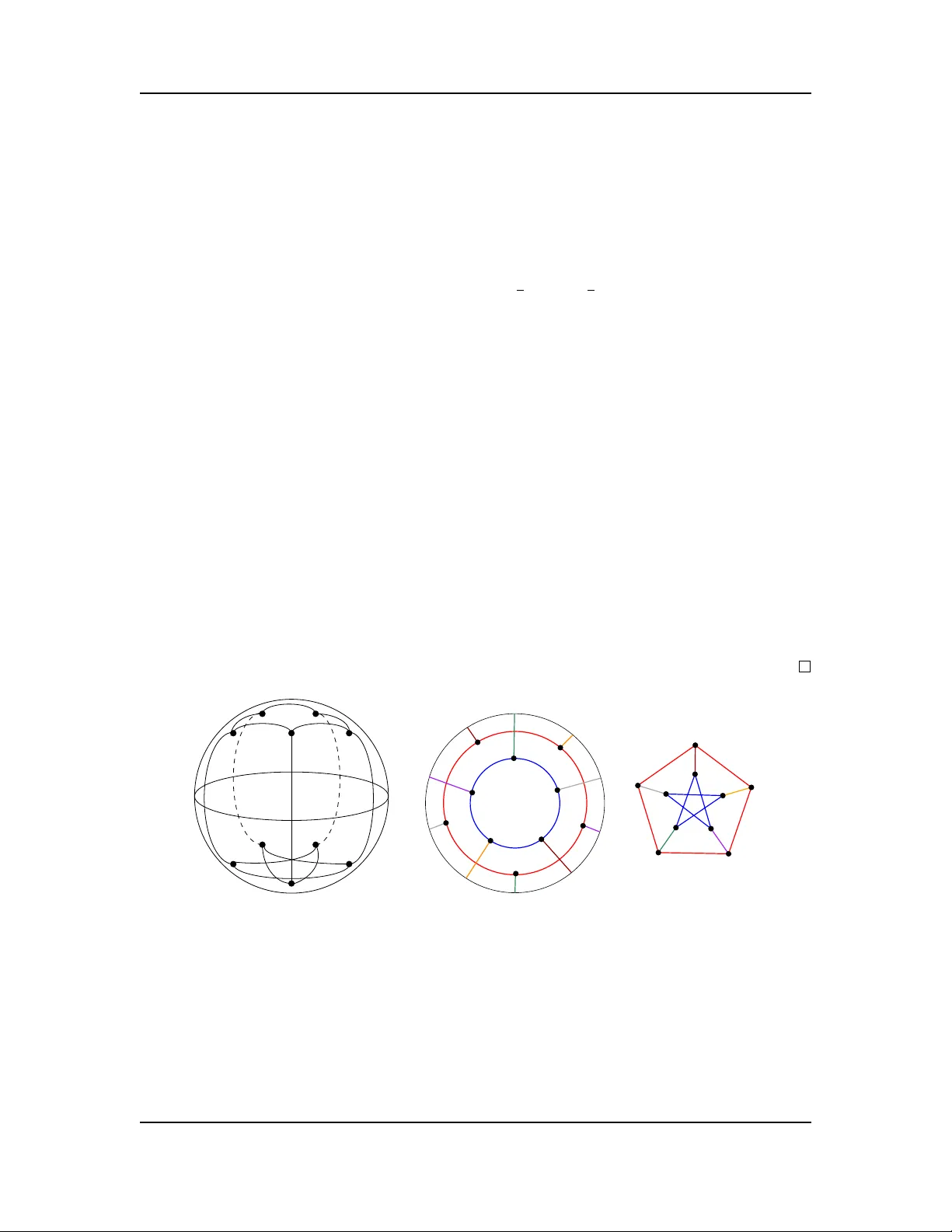
2 -DIMENSIONAL UNIT VE CTOR FL OWS  Hussein Houdrouge Ê , Bobby Miraftab Ê , and P at Morin Ê Abstract . W e study 2 -dimensional unit vector flows on graphs, that is, nowhere-zero flows that assign to each oriented edge a unit vector in R 3 . W e give a new geometric characteri- zation of S 2 -flows on cubic graphs. W e also prove that the class of cubic graphs admitting an S 2 -flow is cl osed under a natural com position opera tion, which yields further construc- tions; in particular , blowing up a vertex into a triangle preserv es the existence of an S 2 -flow . Our second contribution is al gebraic: we extend the rank -based approach of [SIAM J. Dis- crete Math., 29 (2015), pp. 2166–2178] from S 1 -flows to S 2 -flows. More precisely , we show that if an S 2 -flow ϕ satisfies rank( S Q ( ϕ )) ≤ 2 and S Q ( ϕ ) is odd-coordinate-free, then the graph admits a nowhere-zero 4-flow . 1 Introduction In this paper , an oriented graph  G is an undirected graph G = ( V , E ) with two maps init : E − → V and ter : E − → V that assign an initial and a terminal vertex for every edge e ∈ E ( G ). The set E (  G ) denotes the set of oriented edges, that is E (  G ) B { ( e , init( e ) , ter( e )) | e ∈ E ( G ) } . W e will simply refer to an element ( e , init( e ) , ter( e )) ∈ E (  G ) by e . Sometimes, we refer to an oriented graph  G as an orientation of the graph G . For X ⊆ V ( G ), we define E + ( X ) to be the set of all edges e whose init( e ) ∈ X and ter( e ) ∈ V ( G ) ∖ X . The set E − ( X ) is defined as E + ( V ( G ) ∖ X ). For a vertex v ∈ V ( G ), w e write E + ( v ) instead of E + ( { v } ) and E − ( v ) instead of E − ( { v } ). Let A be an additive abelian group, we define a A -circulation over an oriented graph  G as function ϕ : E (  G ) → A that satisfies Kirchho ff ’ s current Law (K CL): X e ∈ E + ( v ) ϕ ( e ) = X e ∈ E − ( v ) ϕ ( e ) (1) for every v ∈ V ( G ). An A -flow for an oriented graph  G is a nowhere zero A -circulation ϕ of  G , that is ϕ ( e ) , 0 for every e ∈ E (  G ). Note that setting ϕ ( e ) = − ϕ ( e ) after swapping init( e ) and ter( e ) will preserve Equation (1) . Thus, if an oriented gr aph  G has an A -fl ow , then an y oriented graph with G as underling graph has an A -flow . Therefore, an undirected graph G has an A -flow if and only if one of its orienta tions  G has an A -flow . For a positive integer k , a Z -flow ϕ for a graph G that satisfies 0 < | ϕ ( e ) | < k for every e ∈ E (  G ) for an orientation  G is called a k -flow . In 1950, T utte proved that having a k -flow is equivalen t to having a Z k -flow , see [ 4 , Theorem 6.3.3]. In [ 11 ], Seymour proves that every  This research was partly funded by NSERC. Ê School of Computer Science, Car leton University . 1 bridgeless graph has a 6-fl ow . Later , al ternative proofs w ere discov ered by DeV os, Rollov á, and Sámal [ 3 ] and DeV os, McDonald, and Nurse [ 2 ]. Howev er , the characterisation of graphs with k -flows for k < 6 remains open. For k = 5, T utte conjectured the following. Conjecture 1 (T utte ’ s 5-flow conjecture) . Every bridgeless gr aph has a 5 -flow . In the definition of A -flow , we can replace the abelian group A by a vector space V to define a vector flow . Since V is an abelian group with respect to the addition operation with identity element being the zero vector , denoted by 0 , vector flow is well defined. In this work, we are interested in vector spaces over R equipped with the E uclidean norm ∥ · ∥ . Let r ≥ 2 be a real number and d a positive integer . An ( r , d ) -flow for a graph G is an R d -flow such that ∥ ϕ ( e ) ∥ lies in the interval [1 , r − 1] for every edge e ∈ E (  G ) for any orientation  G . For r = 2, the (2 , d )-flow is called unit vector flow . Since ev ery element in S d − 1 , the unit sphere of dimension d − 1, is a unit vector in R d , we ref er to (2 , d )-flow by S d − 1 -flow . In order to approach Conjecture 1 , J ain [ 7 ] proposes the following two conjectures that impl y Conjecture 1 . Conjecture 2. Every bridgeless cubic graph has an S 2 -flow . Conjecture 3. There exists a map q : S 2 → {± 1 , ± 2 , ± 3 , ± 4 } such that the antipodal points of S 2 receive opposite values, and any three points which are equidistant on a great circle have values which sum to zero. V ector flows and in particular Conjecture 2 has been studied by several authors, [ 8 , 12 , 13 ]. In this paper , we study S 2 -flow from both geometric and algebraic perspectives. More precisely in order to prove or disprove Conjecture 2 , we provide a new g eometric characterisation for S 2 -flows. W e show that a cubic graph G has an S 2 -flow is equiv alent to having equiangular S 2 -immersion . Informally , an equiangular S 2 -immersion is a mapping of V ( G ) to points in S 2 , and a mapping of E ( G ) to arcs of great circles. The corresponding arcs of edges that are incident to the same vertex are at angle of 2 π / 3 apart from each other . Precisely , we prove the f ollowing. Theorem 1. A cubic graph G admits an equiangular S 2 -immersion if and only if G admits an S 2 -flow . In addition to this char acterisation, we ill ustrate the use of Theorem 1 . W e provide an equiangular S 2 -immersion f or some f amilies including P etersen graph and f or gener alised varia tions of P etersen graph. In Theorem 15 , we show that bipartite graphs are exactly the graphs that admit an equiangular S 2 -immersion to one or two points in S 2 . Finally , we show how to construct graphs with an S 2 -flow from two cubic graphs that have an S 2 -flow , see Theorem 17 . Another interesting question in this area is the foll owing: Problem 1. F or a non-negative integer d , characterize S d -flows for which if G admits an S d - flow with certain properties, then G also admits a nowhere-zero integ er k -flow for some k ≤ 5 . W ang et al. [ 13 ] studied the preceding question for S 1 -flow 2 Lemma 2. [ 13 , Theorem 1.10] If a graph G admits a vector S 1 -flow with r ank at most two, then G admits a nowhere-zero integ er 3 -flow . Here we explain the terminology of vector flows with rank. Suppose V := { ϕ ( e ) | e ∈ E (  G ) } = { v 1 , . . . , v b } . Then for every v i ∈ V , we let E i to be the set of edges with flow val ue equal to v i . For a vertex v ∈ V ( G ), we set ϵ i ( v ) B | E + ( v ) ∩ E i | − | E − ( v ) ∩ E i | . As in [ 13 ], we define the balanced vector ϵ ( v ) of a vertex v ∈ V ( G ) as ϵ ( v ) = ( ϵ 1 ( v ) , . . . , ϵ b ( v ) ) . W e define S Q ( ϕ ) as the span of { ϵ ( v ) | v ∈ V ( G ) } over the field of rational numbers Q . W e say S Q ( ϕ ) is odd-coordinate-free if it con tains no integer vector with exactl y one odd coordinate. W e now are ready to present the extension of [ 13 , Theorem 1.10] to S 2 -flows. Theorem 3. If a graph G admits an S 2 -flow such that S Q ( ϕ ) is odd-coordinate-free of rank at most 2 , then G admits a 4 -flow . 2 Preliminaries First , we start with recalling some basic facts about S 0 -flows. Observa tion 4. F or a graph G , the following statements are equivalent: (i) G has an S 0 -flow . (ii) G has a Z 2 -flow . (iii) All vertices of G have even degree. Thomassen [ 12 ] characterized when a cubic graph admits an S 1 -flow . Let R k denote the set of k t h roots of unity , the set of complex numbers z satisfying z k = 1. Lemma 5 ([ 12 , Proposition 1]) . Let G be a graph. Then the following statements are equivalent: (i) G has a Z 3 -flow . (ii) G has an R 3 -flow . Moreover , both (i) and (ii) imply: (iii) G has an S 1 -flow . If G is cubic, then the three statements (i) , (ii) , and (iii) are equivalent. In this case, G satisfies these conditions if and only if it is bipartite. Note that most of our theorems such as Theorem 1 are phrased in terms of cubic graphs. The reason we focus on cubic graphs is summarized in the following paragraph. Consider the following red uction rules on a graph G . (R1) For every v ∈ V ( G ) with neighbours w 1 , . . . , w 2 k for an integ er k > 1, replace v with v 1 , . . . , v k where each v i for i ∈ { 1 , . . . k } has neighbours w 2 i − 1 , w 2 i . (R2) For ev ery vertex v ∈ V ( G ) with neighbours w 1 , . . . , w 2 k +3 where k is a natural n umber , replace v with vertices v 1 , . . . , v k +1 where v i has neighbours w 2 i − 1 and w 2 i for each i ∈ { 1 , . . . , k } and v k +1 has neighbours w 2 k +1 , w 2 k +2 , and w 2 k +3 see Figure 1 . (R3) For every v ∈ V ( G ) of degree 2, suppress v (replacing v and its two incident edges with a single edge). 3 w 1 w 2 w 2 k +3 w 1 w 2 w 2 k +3 w 2 k +2 w 2 k +1 w 2 k v v 1 v 2 v k v k +1 Figure 1: Splitting a vertex of odd degree. Lemma 6. Let G be a graph and let G ′ be the gr aph ob tained from applying ( R 1) , ( R 2) , and ( R 3) extensively on G , then If G ′ has an A -flow , then G has an A -flow . It is also important to mention the f ollowing corollary for T utte’ s flow polynomial. Proposition 1 ([ 4 ], Corollary 6.3.2) . Given two finite abelian groups A and A ′ with the same order . Then, a graph G has an A -flow if and only if G has an A ′ -flow . Now , we make precise what is discussed in the introduction regarding reversing an edge orienta tion: Observa tion 7. Let  G be an oriented graph, let ϕ : E (  G ) → A for some abelian group A , let  G ′ be obtained from  G by reversing the orientation of some edge e and let ϕ ′ : E (  G ) → A be obtained from ϕ by setting ϕ ′ ( e ) = − ϕ ( e ) . Then ϕ is a A -flow for  G if and only if ϕ ′ is a A -flow for  G ′ . Finally , we recall the f ollowing proposition about the net flow across an y edge cut. Lemma 8. [ 4 , Proposition 6.1.1] Let  G be an oriented graph with an A -circulation ϕ for an abelian group A . Then for any X ⊆ V ( G ) , X e ∈ E + ( X ) ϕ ( e ) = X e ∈ E − ( X ) ϕ ( e ) . The last lemma implies that an y graph with a bridge does not ha ve an A -flow . 3 A Geometric Approach of S 2 -Flows Observa tion 9. Let v 1 , v 2 and v 3 be three unit vectors in R 3 . Then the following two conditions are equivalent: 1. P 3 i =1 v i = 0 ; and 2. the (point set) { 0 , v 1 , v 2 , v 3 } is coplanar and the angle between v i and v j is 2 π / 3 for each 1 ≤ i < j ≤ 3 . In the foll owing, we treat points of S 2 as unit v ectors in R 3 and use 0 := (0 , 0 , 0) to denote the origin in R 3 . For each plane π in R 3 that contains the origin, C π := π ∩ S 2 is called a great circle . Any closed non-empty connected subset A ⊆ C π is called a geodesic arc (in S 2 ). Note that, under this definition, C π is itself a geodesic arc. A geodesic arc A is proper if it a strict subset of some great circle. 4 A simple curve A : [0 , 1] → S 2 in S 2 is a contin uous function with the property that A ( x ) , A ( y ) for each 0 ≤ x < y < 1. For a simple curve A and real numbers 0 ≤ x < y ≤ 1, we use notation A [ x,y ] := { A ( t ) : x ≤ t ≤ y } . A dir ected geodesic arc is a sim ple curve A in S 2 with the property that its image A [0 , 1] is a geodesic arc parameterized so that the length of A [0 ,s ] is equal to s times the length of A [0 , 1] . F or a directed geodesic arc A , the completion of A is the directed geodesic arc C : [0 , 1] → S 2 whose image is a great circle par ameterized so that A [0 , 1] = { C ( t ) : 0 ≤ t ≤ ℓ / 2 π } , where ℓ is the length of A . In other words, the curve C trav erses the great circle C [0 , 1] that contains A [0 , 1] beginning and ending at A (0) and travelling in the same direction as A . In most of what foll ows we will usually not distinguish between a directed geodesic arc A and the (undirected) geodesic arc A [0 , 1] . Let  G be an orienta tion of a graph G . An S 2 -immersion of  G is a function γ with domain V ( G ) ∪ E (  G ) satisfying the following conditions: (i) For each v ∈ V ( G ), γ ( v ) ∈ S 2 . (The vertices of G are mapped to points of S 2 ) (ii) For each v w ∈ E (  G ), γ ( v w ) is a directed geodesic arc A v w with A v w (0) = γ ( v ) and A v w (1) = γ ( w ). (Each directed edge of  G is mapped to a directed geodesic arc in S 2 that begins γ ( v ) and ends at γ ( w ). It is worth noting some di ff erences between S 2 -immersions and embeddings of a graph G in S 2 . Unlike an embedding, there is no requirement that γ : V ( G ) → S 2 . An S 2 -immersion γ may hav e γ ( v ) = γ ( w ) for distinct v , w ∈ V ( G ). Furthermore, unlike a crossing-free embedding, there are no restrictions on the images of edges in an immer - sion. An S 2 -immersion γ ma y hav e γ ( v w ) ∩ γ ( xy ) , ∅ and even γ ( v w ) ⊆ γ ( x y ) for disjoint v w , xy ∈ E (  G ). W e now introduce a notation that allows us to discuss the spherical angle betw een the images of two edges incident to a common v ertex v in an S 2 -immersion. For an S 2 - immersion γ of  G , and a directed edge v w ∈ E (  G ) with A v w := γ ( v w ), we define γ (1 / 3) ( v w ) := A [0 , 1 / 3] v w and γ (1 / 3) ( wv ) := A [2 / 3 , 1] v w . 1 Note that each of γ (1 / 3) ( v w ) and γ (1 / 3) ( wv ) is a proper geodesic arc, even if γ ( v w ) is not. For an orientation  G of a cubic graph G , an S 2 -immersion γ of  G is equiangular if, (iii) for each v ∈ V ( G ) and each pair of undirected edges v x and v y incident to v , the spherical angle between γ (1 / 3) ( v x ) and γ (1 / 3) ( v y ) is exactly 2 π/ 3. W e hav e the following observ ation about S 2 -immersions, akin to Observa tion 7 : Observa tion 10. Let  G be an oriented graph, let γ be an equiangular S 2 -immersion of G , let  G ′ be obtained from  G by reversing the orientation of some edge e and let γ ′ be obtained from γ by setting γ ′ ( e )( t ) := γ ( e )(1 − t ) , for each 0 ≤ t ≤ 1 . Then γ is an equiangular S 2 -immersion of  G if and only if γ ′ is an equiangular S 2 -immersion of  G ′ . 1 The constants 1 / 3 and 2 / 3 are not critical here. The values 1 / 2 ± ϵ for any ϵ > 0 would be su ffi cient. 5 Observa tion 10 implies that if some orientation  G of a cubic graph G has an equiangu- lar S 2 -immersion then every orienta tion of G does. Thus, having equiangular S 2 -immersions is a property of (unoriented) cubic graphs. The following theorem shows that this property completely char acterizes cubic graphs that have S 2 -flows. Theorem 1 . A cubic graph G admits an equiangular S 2 -immersion if and only if G admits an S 2 -flow . Proof. For the forward implication, let γ be an S 2 -immersion of G and fix an arbitrary orientation  G of G . Consider some oriented edge v w ∈ E (  G ), let A v w := γ ( v w ) and let C v w be the completion of A v w . The great circle C v w is contained in a plane π v w ⊂ R 3 , and there are exactly two unit vectors v and − v orthogonal to π v w . If C v w winds counterclockwise around v then we define ϕ ( v w ) := v , otherwise we define ϕ ( v w ) := − v . In either case, C v w , winds counterclockwise around ϕ ϕ ϕ ( v w ). By construction ϕ is a map from E (  G ) to S 2 . W e now argue that ϕ is an S 2 -flow for  G . Consider some vertex v of G . By Observations 7 and 10 we may assume, without loss of generality , that the three edges v v 1 , v v 2 , and v v 3 are oriented awa y from v . W e must therefore show that P 3 i =1 ϕ ϕ ϕ ( v v i ) = 0 . For each i ∈ { 1 , 2 , 3 } , the vector ϕ ϕ ϕ ( v v i ) is orthogonal to the vector γ ( v ), so the vectors ϕ ϕ ϕ ( v v 1 ), ϕ ϕ ϕ ( v v 2 ), and ϕ ϕ ϕ ( v v 3 ) are contained in a plane π v that also contains the origin. By the definition of ϕ ϕ ϕ ( v v i ), π v is orthogonal to the vector γ γ γ ( v ). For each i ∈ { 1 , 2 , 3 } , let A i := γ ( v v i ) and let v i := lim ϵ → 0 A i ( ϵ ) − A i (0) ∥ A i ( ϵ ) − A i (0) ∥ . In words, v i is the unit vector that is parallel to the direction in which A i departs from γ ( v ). The spherical angle between γ (1 / 3) ( v v i ) and γ (1 / 3) ( v v j ) is equal to the angle between the two vectors v i and v j , f or each 1 ≤ i < j ≤ 3. For each i ∈ { 1 , 2 , 3 } , the vector v i is contained in the plane π v and is, in fact, obtained by rotating ϕ ϕ ϕ ( v v i ) clockwise around γ γ γ ( v ) by an angle of π / 2. Therefore, the angle between ϕ ϕ ϕ ( v v i ) and ϕ ϕ ϕ ( v v j ) is equal to the angle between v i and v j . Since γ is equiangular , this angle is 2 π / 3. Therefore ϕ ϕ ϕ ( v v 1 ), ϕ ϕ ϕ ( v v 1 ), and ϕ ϕ ϕ ( v v 2 ) are coplanar with the origin and the angle between ϕ ϕ ϕ ( v v i ), and ϕ ϕ ϕ ( v v j ) is 2 π/ 3, for each 1 ≤ i < j ≤ 3. Therefore, Observ ation 9 implies that P 3 i =1 ϕ ϕ ϕ ( v v i ) = 0 , as required. T o establish the backward implication, fix an arbitrary orientation  G of G and let ϕ be an S 2 -flow of  G . For each vertex v of G arbitrarily select one of the two possible cyclic orders on the three edg es of G incident to v . W e use v 1 , v 2 , v 3 to denote the neighbours of v , using this cyclic order . Now consider an arbitrary v ertex v of G . By Observation 7 we ma y assume, without loss of gener ality , tha t the three edg es v v 1 , v v 2 , and v v 3 are oriented aw ay from v . Define γ γ γ ( v ) B (2 / √ 3)( ϕ ϕ ϕ ( v v 1 ) × ϕ ϕ ϕ ( v v 2 )). By Observation 9 , the angle between the vectors ϕ ϕ ϕ ( v v 1 ) and ϕ ϕ ϕ ( v v 2 ) is 2 π / 3, so γ ( v ) is a unit v ector (since sin(2 π/ 3) = √ 3 / 2). Also by Observa tion 9 , v 1 , v 2 , and v 3 are coplanar with the origin, so γ γ γ ( v ) = 2 / √ 3 ϕ ϕ ϕ ( v v 2 ) × ϕ ϕ ϕ ( v v 3 ) = 2 / √ 3 ϕ ϕ ϕ ( v v 3 ) × ϕ ϕ ϕ ( v v 1 ) This defines γ ( v ) for each vertex v of G . What remains is to define γ ( u v ) for each edge u v ∈ E(  G ). Without loss of generality , assume that u = v 1 and that v = u 1 . By Observ ation 7 we may assume, without loss of 6 generality , that u u 2 , u u 3 , u v , v v 2 , v v 3 are the five (oriented) edges of  G incident to u and v . Then γ γ γ ( u ) = 2 / √ 3( ϕ ϕ ϕ ( u v ) × ϕ ϕ ϕ ( u u 2 )) and γ ( v ) = − 2 / √ 3( ϕ ( u v ) × ϕ ( v v 2 )). Geometrically , this means that γ ( u ) and γ ( v ) are each contained in the plane π u v that contains the origin and is orthogonal to ϕ ( u v ). Let C u v := π u v ∩ S 2 , so C u v is a great circle that contains γ ( u ) and γ ( v ). W e define γ ( u v ) to the directed arc A u v that is contained in C u v , has A u v (0) = γ ( u ), A u v (1) = γ ( v ) and whose extension winds counterclockwise around γ γ γ ( u v ). W e now argue that γ is an S 2 -immersion of G . By definition, γ ( v ) ∈ S 2 for each v ∈ V ( G ), so γ satisfies Condition (i) . By definition, each edge u v of  G is mapped to a directed geodesic arc A u v (contained in C u v ) with A u v (0) = γ ( u ) and A u v (1) = γ ( v ), as required by Condition (ii) . Therefore γ is an S 2 -immersion. All that remains is to show that γ is equiangular . Let v be an arbitrarys vertex of G . By Observation 7 we may assume without loss of generality , that v v 1 , v v 2 , and v v 3 are the three orien ted edges of  G incident to v . Since γ is a S 2 -flow , P 3 i =1 ϕ ( v v i ) = 0 . By Observation 9 , there is a plane π v that contains { 0 , ϕ ( v v 1 ) , ϕ ( v v 2 ) , ϕ ( v v 3 ) } . By the choice of γ ( v ), this plane is orthogonal to the vector γ γ γ ( v ). For each i ∈ { 1 , 2 , 3 } , let A i := γ ( v v i ) and let C i be the completion of A i . Then, for each i ∈ { 1 , 2 , 3 } , the tangent vector v i := lim ϵ ↓ 0 ( C i ( ϵ ) − C i (0)) ∥ C i ( ϵ ) − C i (0) ∥ is contained in the plane π v and is, in fact , obtained by rotating ϕ ϕ ϕ ( v v i ) clockwise around γ γ γ ( v ) by an angle of π / 2. Therefore, the angle betw een v i and v j is equal to the angle between ϕ ϕ ϕ ( v v i ) and ϕ ϕ ϕ ( v v j ), for each 1 ≤ i < j ≤ 3. By Observation 9 this latter angle is 2 π/ 3. Therefore the spherical angle betw een γ (1 / 3) ( v v i ) and γ (1 / 3) ( v v j ) (which is equal to the angle between v i and v j ) is 2 π / 3. Therefore γ satisfies Condition (iii) , so γ is an equiangular S 2 -immersion of  G . 4 Examples of Graphs with an S 2 -Flows In this section, we illustr ate the use of Theorem 1 to show that some graphs admits an S 2 -flow . An important tools to accomplish our objective is the Intermediate V alue Theo- rem . Thus, we begin by recalling this fact about continuous functions. A space S is path- connected , if for ev ery pair of points x and y in S , there exists a continuous function γ : [0 , 1] → S such that γ (0) = x and γ (1) = y . (2) Lemma 11. [Intermediate V alue Theorem] Let S be a path-connected space, and let f : S → R be a continuous function. If a, b ∈ S then f attains all the values between f ( a ) and f ( b ) . The next lemma describes a local modification tha t preserves the immersion. 7 Lemma 12. Let G be a graph with an S 2 -immersion. Then, for any vertex v ∈ V ( G ) , we can replace v with the antipodal point − v and modify only the edges incident to v to obtain another S 2 -immersion of G that preserves the angles formed by any pair of edges meeting at a common vertex. Proof. The great circles that contain the edges incident to v intersect both at v and at − v . For each such edg e v w , we replace it with the arc of the same great circle tha t connects − v to w , choosing the arc that contains the original edge v w . T o see that this transformation preserves the angles betw een edges incident to v , observe that this can be visualized as moving the point v along the grea t circle, away from w , until it reaches the antipodal point − v . This operation e ff ectively reverses the direction in which each edge v w departs from v . Since the direction of each incident edge is negated, the angles between any pair of them remain unchanged. This operation does not a ff ect the direction of any edge at its other endpoint. In particular , for each neighbor w of v , the direction in which the edge wv departs from w remains unchanged. Therefore, the resulting immersion preserves all l ocal geometric properties at each v ertex, and in particular , all angles at the vertices remain the same. 4.1 Generalised P eterson Graph Let a, b, p ∈ N with l p 6 m ≤ a, b ≤ j p 2 k . W e define the quasi-P etersen graph G a,b,p with parame- ters a, b , p , as follows. 1. The vertex set is the disjoint union of V B { v 0 , . . . , v p − 1 } and W B { w 0 , . . . , w p − 1 } , 2. The edge set E ( G a,b,p ) = C V ∪ C W ∪ M , where (all subscripts are taken mod ulo p , and [ p ] := { 0 , 1 , . . . , p − 1 } ) C V B { v i v i + a : i ∈ [ p ] } , C W B { w i w i + b : i ∈ [ p ] } , M B { v i w i : i ∈ [ p ] } . Observa tion 13. The following holds true: 1. One can verify that G 1 , 2 , 5 is the P etersen graph. More precisely if gcd( a, p ) = 1 then C V is a cycle. Similarly , gcd( b , p ) = 1 implies that C W is a cycle. In particular , for any prime p , taking a = ⌊ p / 2 ⌋ − 1 and b = ⌊ p / 2 ⌋ yields a graph G a,b,p consisting of two cycles C V and C W with a matching M between them. 2. F or any odd p ≥ 5 , the choices a = ⌊ p / 2 ⌋ − 1 and b = ⌊ p/ 2 ⌋ satisfy p 6 < a, b < p 2 . 3. F or any even p ≥ 8 , the choices a = p / 2 − 2 and b = p/ 2 − 1 satisfy this r equirement. 4. The generlized P etersen graph G ( n, k ) 2 is a graph with vertex set { u 0 , u 1 , . . . , u n − 1 , v 0 , v 1 , . . . , v n − 1 } 2 Here we use the W atkins’ notation. Howev er , some authors use the notation GP G ( n, k ). 8 and edge set { u i u i +1 , u i v i , v i v i + k | 0 ≤ i ≤ n − 1 } where subscripts are to be read modulo n and where k < n/ 2 . One can see that our notation generalizes the notion of a generalized P etersen graph, wher e gcd( a, p ) = 1 . W e say tha t an S 2 -immersion is injective if the vertex map γ ↾ V ( G ) : V ( G ) → S 2 is injec- tive. Proposition 2. F or any positive integers a, b , p with p 6 < a, b < p 2 , the graph G a,b,p has an injec- tive equiangular S 2 -immersion. Proof . Place the v ertices of V = V ( G a,b,p ) a t the vertices of a regular p -gon in the plane and draw the edges of C V as straight -line segments. This gives a collection of cycles in which the internal angle at each vertex is less than 2 π / 3 (because p / a < 6). Similarly , place the vertices of W at the vertices of a regular p -gon and draw the edges of C W as straight -line segments; again, the internal angle at each vertex is less than 2 π/ 3 (because p / b < 6). W e start with the vertices of V equally spaced on the equator of S 2 and place the vertices of W so that w i coincides with v i for each i ∈ [ p ]. Move the vertices of V toward the north pole until C V is drawn with all vertices on a small circle C and with internal angles 2 π / 3 at each vertex. Since C V is invariant under the map v i 7→ v i +1 , the angle formed by C and the edge v i v i − a equals the angle formed by C and v i v i + a , for ev ery i ∈ [ p ]. Next, move the vertices of W toward the south pole until C W is drawn with internal angles 2 π / 3. W e now have a configuration with v i directly “ above ” w i for each i ∈ [ p ]. A t each v i , the three edges v i v i − a , v i v i + a , and v i w i meet at 2 π / 3 angles; similar ly , at each w i , the three edges w i w i − b , w i w i + b , and w i v i meet at 2 π / 3 angles. Theref ore we obtain an S 2 -immersion of G a,b,p in which all vertices map to distinct poin ts. (a) (b) Figure 2: T wo di ff erent equiangular S 2 -immersion of the P etersen graph. 4.2 S 2 -immersion to One and T wo Points In this section, w e char acterise the graphs that admit an equiangular S 2 -immersion to exactly one or two points. W e begin by showing that an y equiangular S 2 -immersion to two points is an equiangular S 2 -immersion to antipodal points. 9 Lemma 14. Let G be a cubic graph with two-points equiangular S 2 -immersion γ that is γ ( V ( G )) = { p, q } , then the points q and p are antipodal. Proof. Since γ is a two-point S 2 -immersion, there exists at least one vertex v ∈ V ( G ) such that γ ( v ) = p , and one of its three neighbours x , y or z that γ sends to q , otherwise we do not hav e two-points equiangular S 2 -immersion. W e have two cases. Case (1) : A t least two of γ ( x ) , γ ( y ), and γ ( z ) equals to q , say x and y . Since γ is an equiangular S 2 -immersion the arcs γ ( v x ) and γ ( v y ) belong to two distinct great circles that intersect in p and q . Any two distinct great circles intersect at antipodes. Thus, q = − p . Case (2) : Exactly one of γ ( x ) , γ ( y ), and γ ( z ) is equal to q , sa y x . Moreover , suppose q , − p , otherwise, we are done. Let C be the grea t circle containing γ ( v x ). In this case, an y point of C ∖ p satisfies the conditions of equiangular S 2 -immersion for the edge e = v x . Let G q be the union of γ ( e ) for e = u w ∈ E ( G ) such that γ ( u ) = γ ( w ) = q and γ ( u ) = p, γ ( w ) = q ; That ’ s it G q is the drawing of the subgraph of G whose at least one of its edges’ endpoints is mapped to q . Let R be a rotation tha t sends q to − p al ong the shortest arc betw een q and − p . Apply R to every point in G q . Since R is an isometry , R preserves the angles between any arc from q to q . For an y arc going from p to q , we can replace it by an arc from p to − p while preserving its direction along C . Since the arc from p to q did not change angles with the arcs going out of p , it preserves the fact tha t γ is an equiangular S 2 -immersion. Now , we are ready to show that bipartite graphs are exactly the graphs that have one or two points equiangular S 2 -immersion. In order to prov e the next theorem, we make use of the following w ell known fact about regular bipartite graphs. Proposition 3. [ 4 , Corollary 2.1.3.] Every k -regular ( k ≥ 1) bipartite graph has a perfect matching. Theorem 15. Let G be a cubic graph. Then the following statements are equivalent. (a) G has a one-point equiangular S 2 -immersion. (b) G has a two-point equiangular S 2 -immersion. (c) G is bipartite. Proof. For the direction ( a ) = ⇒ ( b ), by applying Lemma 12 to any v ∈ V ( G ), we get an S 2 -immersion. For the reverse direction ( b ) = ⇒ ( a ), suppose we hav e a two-point S 2 -immersion γ , by Lemma 14 γ in an “ antipodal S 2 -immersion ”. Then, applying Lemma 12 to vertices that are mapped to one of the antipodes giv e us a one-point S 2 -immersion. Now , we prov e ( c ) ⇐ ⇒ ( b ). For the f orward direction, consider a cubic bipartite gr aph G = ( A ∪ B, E ). Let − → G be an orientation of G such that every edge e = ab ∈ E ( G ) with a ∈ A and b ∈ B , e is oriented from a to b . W e want to construct a two-point S 2 -immersion γ . Let p be any point in S 2 . Set γ ( a ) = p for ev ery a ∈ A and γ ( b ) = − p for every b ∈ B . Furthermore, let C 1 , C 2 , and C 3 be three great circles with the smallest angle between any of them equals to π/ 3. Precisely , we have six geodesic arcs from p to − p along C 1 , C 2 , and C 3 . Choose three of them at a distance 2 π / 3, call them C ′ 1 , C ′ 2 , and C ′ 3 . Note that C ′ i (0) = p 10 to C ′ i (1) = − p f or 1 ≤ i ≤ 3. Since G is cubic bipartite graph, by Proposition 3 w e hav e three perfect matchings M 1 , M 2 , and M 3 . For every e i = ab ∈ M i , let γ ( − → e i ) = C ′ i . Now at a vertex a ∈ A , the outgoing edges each belongs to exactly one of the M i , and its corresponding arc is at 2 π / 3 from the other ones. Similar ly f or ev ery v ertex b ∈ B . In other words, for each vertex a ∈ A with neighbors b 1 , b 2 , and b 3 , the spherical angle between γ (1 / 3) ( ab i ) and γ (1 / 3) ( ab j ) for i , j ∈ { 1 , 2 , 3 } and i , j is equal to 2 π/ 3 since each of γ ( ab i ) ⊂ C ′ j for some j ∈ { 1 , 2 , 3 } . Similar argument applies for the arcs around the v ertices of B . For the backward direction, suppose we hav e a two-point S 2 -immersion γ of a cubic graph G . By Lemma 14 , we can assume that γ ( V ( G )) = { p , − p } for some p ∈ S 2 . Note that any great circle C that contains p and − p is contained in a plane π C ⊂ R 3 whose normal vector v is perpendicular to the line defined by { p, − p } . The set of these normal vectors defines are subset of a circle S ⊂ S 2 . By similar reasoning of the proof of Theorem 1 , G has an S 2 -flow whose val ues belongs to the circle S . In other words, G has an S 1 -flow . Since G is cubic and has S 1 -flow , by Lemma 5 G is bipartite. Using Lemma 5 , we can concl ude with the following corollary . Corollary 16. F or a cubic graph G , the followings are equivalent, 1. T wo-point S 2 immersion. 2. 3 -flow . 3. R 3 -flow . 4. S 1 -flow . 4.3 Combining Cubic Graphs with S 2 -flows Let v be a vertex in a graph G such that v has k neighbours. W e define vertex splitting at v by replacing v with k v ertices, v 1 , ..., v k . Each vertex v i for 1 ≤ i ≤ k inherits exactly one neighbour of v . In other words, we replaced v with k leaves, each is attached to one of its neighbour . Given two gr aphs G and H such that each contains a v ertex of degree k f or some k ∈ N . W e define injecting H into G at a v ertex v ∈ V ( G ) of degree k as follow . First, w e perform a vertex splitting on v and on a vertex w ∈ V ( H ) of the same degree. Now , w e hav e k lea ves in G , v 1 , ..., v k and k lea ves in H , w 1 , ..., w k . For each 1 ≤ i ≤ k , w e identify v i in G to the unique neighbour of w i in H , and identify w i to the unique neighbour of v i in G , we suppress the identified v ertex to form an edge. W e denote the new graph as H ▷ G . Theorem 17. Let G and H be two cubic graphs with S 2 -flows g and h respectively . Then, the graph H ▷ G created by injecting H into a vertex v of G has an S 2 -flow . Proof. Let w be a v ertex of H , as d ( w ) = d ( v ) = 3 injecting H into G at v is well defined. Let a, b , and c be the vectors in S 2 that g maps the incident edges at v to. Since g is a flow , we hav e a + b + c = 0. By Observa tion 9 , a, b, and c are coplanar with angle 2 π/ 3 between them. Similarl y , let a ′ , b ′ and c ′ be the v ectors in S 2 that h maps the edges around w to. Note that there is bijection that maps { a ′ , b ′ , c ′ } to { a, b , c } , precisely this bijection is a rotation of normal vectors containing { a ′ , b ′ , c ′ } to the normal v ector of the plane containing { a, b , c } . 11 Then, it follow ed by another rotation to align the vector a ′ to a . Denote this rotation by θ . Now , we define f from E ( H ▷ G ) as f ( e ) = g ( e ) for e ∈ E ( H ▷ G ) ∖ E ( H ), and f ( e ) = θ ◦ h ( e ) for e ∈ E ( H ). It is clear that at every vertex of V ( G ) ∩ V ( H ▷ G ) the flow conditions holds for f . For every v ertex w ∈ V ( H ) ∩ V ( H ▷ G ), f ( e 1 ) + f ( e 2 ) + f ( e 3 ) = θ ◦ g ( e 1 ) + θ ◦ g ( e 2 ) + θ ◦ g ( e 3 ) = θ ◦ ( g ( e 1 ) + g ( e 2 ) + g ( e 3 )) (by the linearity of θ ) = 0 where e 1 , e 2 , e 3 are the edges incident to w . Lemma 18. The complete graph K 4 has an equiangular S 2 -immersion, consequently an S 2 -flow . Proof. W e wan t to define an S 2 -immersion γ for K 4 . Let v 0 , v 1 , v 2 , and v 3 be the four vertices of K 4 , and set γ ( v 0 ) = (0 , 0 , 1). Then, place v 1 , v 2 , and v 3 at equal distance from each other at the equatorial; the great circle C π defined by the intersection of S 2 and the plane π with zero z -coordinate. Let γ ( v i ) for i ∈ { 1 , 2 , 3 } be defined as described above. Between any consecutive γ ( v i ) for i ∈ { 1 , 2 , 3 } draw an arc along C π (this arc corresponds to the shortest possible arc), this arc between γ ( v i ) and γ ( v j ) corresponds to the edge v i v j for i , j and i , j ∈ { 1 , 2 , 3 } . Between γ ( v 0 ) and γ ( v i ) for i ∈ { 1 , 2 , 3 } draw an arc along the unique great circle containing γ ( v 0 ) and γ ( v i ), call such circle C v 0 v i . Note that γ is not an S 2 -immersion as it is defined now; the angle between γ ( v i v 0 ) and γ ( v i v j ) for i , j ∈ { 1 , 2 , 3 } is π/ 2, and the angle between γ ( v i v j ) and γ ( v i v k ) is equal to π . T o make γ an S 2 -immersion, we are going to move at a constant speed each of the γ ( v i ) for i ∈ { 1 , 2 , 3 } toward − γ ( v 0 ) along C v 0 v i as defined abov e. As this movemen t is going extend the arc of γ ( v 0 v i ) to the new position of γ ( v i ) f or i ∈ { 1 , 2 , 3 } . As the γ ( v i ) for i ∈ { 1 , 2 , 3 } approaches − γ ( v 0 ), the angles between the γ ( v i )s is approaching π / 3. By the intermediate val ue theorem, as the angle between γ ( v i )s changes between π and π / 3 there must be a position in which the γ ( v i )s attain an angle of 2 π/ 3; let such a position be the final position of each of the γ ( v i ) for i ∈ { 1 , 2 , 3 } . It remains to show that the angle between γ ( v i v 0 ) and γ ( v i v j ) for i , j ∈ { 1 , 2 , 3 } is 2 π / 3. By the symmetry of movement , as γ ( v i ) for i ∈ { 1 , 2 , 3 } is moving toward − γ ( v 0 ) as it is described above, the angle betw een the arc joining γ ( v 0 ) to γ ( v i ) and the arcs joining γ ( v i ) to its right and left neighbors is increasing by the same amount. Therefore, the arc γ ( v 0 v i ) remain an angular bisector for the angle γ ( v j ) γ ( v i ) γ ( v k ); consequently at the final position the val ue of γ ( v k ) γ ( v i ) γ ( v 0 ) equals to (2 π − 2 π / 3) / 2 = 2 π / 3. In the following, blowing up a vertex in a cubic graph by a triangle is to replace the vertex by a cycle of length three and giv e exactly one neighbour to each of its vertex. Theorem 19. Let G be a cubic graph. If G admits an S 2 -flow , then the gr aph obtained by blowing up any vertex in V ( G ) into a triangle also admits an S 2 -flow . Proof. Blowing up a vertex v in V ( G ) in to a triangle is equivalent to injecting K 4 into v . By Lemma 18 and Theorem 17 , the conclusion f ollows. 12 5 An Algebraic Approach of S 2 -Flows W ang et al. [ 13 ] proved the following: Lemma 20. [ 13 , Theorem 1.10] If a graph G admits a vector S 1 -flow with rank at most two, then G admits a 3 -flow . In this section, we generalize the previous result to S 2 under a mild assumption. Let ϕ ϕ ϕ be a S 2 –flow on a graph G . Its set of flow v alues is { ϕ ϕ ϕ ( e ) | e ∈ E ( G ) } = {± v 1 , . . . , ± v b } , where { v 1 , . . . , v b } ⊆ S 2 consists of b pairwise linearly independent vectors. Without loss of generality we may further assume that { ϕ ϕ ϕ ( e ) | e ∈ E ( G ) } = { v 1 , . . . , v b } , because whenever an edge e satisfies ϕ ϕ ϕ ( e ) = − v i we simpl y reverse the orientation of e and replace its flow value by − ϕ ϕ ϕ ( e ) = v i . For a vertex v , define the balanced vector ϵ ( v ) ∈ Z b as: ϵ ( v ) = ( ϵ 1 ( v ) , . . . , ϵ b ( v ) ) , where ϵ i ( v ) = | E + ( v ) ∩ E i | − | E − ( v ) ∩ E i | , and E i is the set of edges with flow value v i . The balanced equation at a v ertex v is defined as ϵ 1 ( v ) v 1 + · · · + ϵ b ( v ) v b = 0 , (3) Let S ( ϕ ) denote the linear subspace of R b genera ted by all balanced vectors of the flow ϕ over R . The r ank of this subspace, denoted by rank( ϕ ), is called the rank of the S 2 -flow ϕ . W ang et al. [ 13 ] proved that G admits a nowhere-zero integer 3-flow if G admits a vector S 1 -flow with rank at most two. This result is sharp since there are examples that admit vector S 1 -flows with rank a t least 3, but no nowhere-zero integer 3-flows. Let V = Q b be the vector space over Q . W e define S Q ( ϕ ) to be the linear subspace of Q b genera ted by all balanced vectors. W e call a subspace W of V an odd-coordinate-free if it contains no integ er vector with exactly one odd coordinate. The following lemma is known as the finite-dimensional Riesz representation theo- rem. Lemma 21. [ 6 , Sec.8.3 Theorem 6] If ( V , ⟨ ∗ , ∗⟩ ) is a finite-dimensional inner product space over a field F and f is a linear functional on V (i.e f : V → F ), then there exists a unique vector β ∈ V such that f ( α ) = ⟨ α , β ⟩ for all α ∈ V . If V is a v ector space ov er a field F , a hyperspace in V is a maximal proper subspace of V . Lemma 22. [ 6 , Sec.3.6 Theorem 19] If f is a non-zero linear functional on the vector space V over a field F , then the kernel of f is a hyperspace in V . Conversely , every hyperspace in V is the kernel of a (not unique) non-zero linear functional on V . Although the foll owing result is known, we provide a proof for com pleteness and the reader’ s conv enience. 13 Lemma 23. Let V be a finite-dimensional vector space over F with a proper subspace W . If v < W , then there exists a hyperspace(maximal subspace) M with W ⊆ M ⊊ V and v < M . Proof. Let { w 1 , . . . , w k } be a basis of W . Since v < W , the set { w 1 , . . . , w k , v } is linearly in- dependent and can be extended to a basis of V , say B = { w 1 , . . . , w k , v , u k +2 , . . . , u n } . Define f ∈ V ∗ by prescribing its val ues on B : f ( w i ) = 0 (1 ≤ i ≤ k ) , f ( v ) = 1 , f ( u j ) = 0 ( k + 2 ≤ j ≤ n ) , and extend f linearly to all of V . Since f vanishes on W , we conclude that W is subset of the kernel of f . Furthermore by definition f ( v ) = 1 which implies v < ker( f ). Now it follows from Lemma 22 tha t ker( f ) is a hyperspace. Next we define the support of a vector . Let x = ( x 1 , . . . , x n ) be a v ector in a v ector space V . The support of x is supp ( x ) B { i ∈ [ n ] | x i , 0 } . It is a well-known fact that in any binary linear code, either all codewords have even weight , or exactly half of them do. Lemma 24. A k -dimensional binary subspace V ⊆ Z n 2 has either 0 or exactly 2 k − 1 vectors of odd support. Let ( V , ⟨∗ , ∗⟩ ) be a vector space equipped with an inner product. If W is a subspace of V , it is not necessarily true that dim( W ⊥ ) + dim( W ) = dim( V ), where W ⊥ is the orthogo- nal complement of W . Howev er , if the inner product is non-degenerate , then the equality dim( W ⊥ ) + dim( W ) = dim( V ) does hold. In particular , the standard inner product on Z n 2 is a non-degenera te. The following lemma pla ys a crucial role in this section. Lemma 25. Let V ⊆ Z n 2 be a linear subspace of dimension d with n − 2 ≤ d ≤ n . If for each coordinate i = 1 , . . . , n , the projection map π i : V → Z 2 , is surjective. Then there exist two vectors x , y ∈ V such that ( π i ( x ) , π i ( y )) , (0 , 0) for every i . Proof. Let V ⊥ = { w ∈ Z n 2 | w · v = 0 for all v ∈ V } be the orthogonal com plement of V . Then dim( V ⊥ ) = k = n − d ∈ { 0 , 1 , 2 } , since n − 2 ≤ d ≤ n . The surjectivity of each π i implies that no standard basis e i lies in V ⊥ ; consequentl y , ev ery nonzero w ∈ V ⊥ satisfies | supp( w ) | ≥ 2. Assume, for the sake of contradiction, that the lemma is false. Then w e ha ve the following: F or any pair of vectors x , y ∈ V , there exists an index i ∈ [ n ] such that x i = y i = 0 . (4) For x ∈ V define the zero set Z x = { i ∈ [ n ] | x i = 0 } . W e now claim the following: Claim 26. for every x ∈ V , there exists a non-zero vector w ∈ V ⊥ with odd support such that supp ( w ) ⊆ Z x . Proof of Claim: Let us fix an arbitrary vector x ∈ V . Without loss of generality , w e can assume that Z x = [ | Z x | ]. Our hypothesis, applied to this specific x , implies that for any vector y ∈ V , there is an index i ∈ Z x , where y i = 0. This means that no vector in V has a 14 ‘1’ in all coordinate positions of Z x . Next, w e consider the projection map from V onto the coordinates in Z x : π Z x : V → Z | Z x | 2 B Z 2 × · · · × Z 2 | {z } | Z x | Since no vector in V has a ‘1’ in all coordinate positions of Z x , we infer that the all-ones vector 1 ∈ Z | Z x | 2 is not in the image of π Z x and so the projection π Z x is not a surjective map. It follows from Lemma 23 that there is a hyperspace(maximal subspace) M of Z | Z x | 2 such that Im ( π Z x ) ⊆ M and 1 < M . By Lemma 22 , let f : Z | Z x | 2 → Z 2 be the linear functional such that the kernel of f is M . W e now in voke Lemma 21 and conclude that the non-zero linear functional f can be represented by the dot product with a non-zero v ector u ∈ Z | Z x | 2 . By definition of f , we ha ve the following tw o crucial properties: 1. u · v = 0 for all v ∈ Im ( π Z x ), as Im ( π Z x ) is a subset of the kernel of f . 2. u · 1 = 1, as 1 does not belong to kernel of f . Hence it implies that | supp ( u ) | is odd. W e extend u to a v ector w ∈ Z n 2 by setting its com ponents to 0 for all coordinates not in Z x . By construction, supp( w ) = supp( u ), so supp( w ) ⊆ Z x and | supp( w ) | is odd. The first condition saying that u · v = 0 for all v ∈ Im ( π Z x ). By extending the vector u to the vector w , we deduce that w · y = 0 for all y ∈ V , which means w ∈ V ⊥ and the claim is proved. Let V ⊥ od d = { w ∈ V ⊥ ∖ { 0 } | | supp ( w ) | is odd } . For each w ∈ V ⊥ od d , define the subspace V w B { v ∈ V | supp( v ) ∩ supp( w ) = ∅} . W e now claim the following: Claim 27. V = [ w ∈ V ⊥ od d V w Proof of Claim: It foll ows from Claim 26 that for ev ery v ∈ V , there exists a non-zero vector w ∈ V ⊥ with odd support such that supp ( w ) ⊆ Z v . Recall that by definition, Z v is the set of indices i ∈ [ n ] for which the i -th coordinate of v is zero. In particular , this means that supp ( v ) ∩ Z v = ∅ . Hence, we conclude tha t v ∈ V w . By Lemma 24 , we know that the number of vectors in V ⊥ od d is either 0 or 2 k − 1 , where k = dim( V ⊥ ). • Case k = 0 ( d = n ): V ⊥ = { 0 } , and so V ⊥ od d is empty and V = Z n 2 . Claim 27 yields a contradiction. • Case k = 1 ( d = n − 1 ): | V ⊥ od d | ≤ 2 1 − 1 = 1. The cov ering becomes V = V w , where w lies in V ⊥ od d . This means that the support of each vector of V has empty intersection with supp ( w ). In other words, all vectors in V are zero on supp ( w ), which violates the surjectivity of the projection maps π i for i ∈ supp ( w ). 15 • Case k = 2 ( d = n − 2 ): | V ⊥ od d | ≤ 2 2 − 1 = 2. The covering becomes V = V w 1 ∪ V w 2 which gives us a con tradiction. Since every possible case arising from our initial assum ption leads to a contradiction, the assumption must be false. Therefore, there must exist two vectors x , y ∈ V such that supp( x ) ∪ supp( y ) = { 1 , . . . , n } . Theorem 3 . If G admits an S 2 -flow such that S Q ( ϕ ) is odd-coordinate-free of rank at most 2 , then G admits a 4 -flow . Proof. Let f be an S 2 -flow on a graph G with rank r ≤ 2. The set of flow v alues is { v 1 , . . . , v b } ⊆ S 2 . By definition, for any vertex v ∈ V ( G ), its balanced vector ϵ ( v ) = ( ϵ 1 ( v ) , . . . , ϵ b ( v )) sat - isfies the K CL for the S 2 -flow: P b i =1 ϵ i ( v ) v i = 0. Our goal is to construct a nowhere-zero 4-flow . By a classic result of T utte, this is equivalent to constructing a nowhere-zero flow using the Klein four -group, Z 2 × Z 2 . A function ϕ : E ( G ) → Z 2 × Z 2 ∖ { 0 } is a nowhere-zero Z 2 × Z 2 -flow if the K CL holds at every vertex. Since every element in Z 2 × Z 2 is its own inv erse, the K CL simplifies to: X e incident to v ϕ ( e ) = 0 (in Z 2 × Z 2 ) W e shall define a flow ϕ by assigning a value g i ∈ Z 2 × Z 2 ∖ { 0 } to all edges with the flow vector v i . That is, if an edg e e has f ( e ) = v i , w e set ϕ ( e ) = g i . The K CL f or ϕ at a v ertex v is then: b X i =1 ( | E + ( v ) ∩ E i | − | E − ( v ) ∩ E i | ) g i = b X i =1 ϵ i ( v ) g i = 0 Let ϵ ϵ ϵ ′ ( v ) = ( ϵ 1 ( v ) mod 2 , . . . , ϵ b ( v ) mod 2) ∈ ( Z 2 ) b B Z 2 × · · · × Z 2 | {z } b times . The condition becomes: b X i =1 ϵ ′ i ( v ) g i = 0 ⇔ ϵ ′ ( v ) · ( g 1 , . . . , g b ) = 0 (in Z 2 × Z 2 ) This equation must hold for all v ∈ V ( G ). Let S ′ ⊆ ( Z 2 ) b be the subspace spanned by all vectors { ϵ ′ ( v ) } . W e know that k = dim Z 2 ( S ′ ) ≤ dim Q S ( f ) ≤ 2. Furthermore we can repre- sent elements of Z 2 × Z 2 as vectors in ( Z 2 ) 2 . Let g i = ( x i , y i ), where ( x i , y i ) ∈ ( Z 2 ) 2 ∖ { (0 , 0) } . The vector equation P ϵ ′ i ( v ) g i = 0 decomposes into two independent linear equations over Z 2 : ϵ ϵ ϵ ′ ( v ) · ( x 1 , . . . , x b ) = 0 ϵ ϵ ϵ ′ ( v ) · ( y 1 , . . . , y b ) = 0 These m ust hol d for all v . This is equivalent to requiring the v ectors x = ( x 1 , . . . , x b ) and y = ( y 1 , . . . , y b ) to lie in the orthogonal complement of S ′ , denoted W = ( S ′ ) ⊥ . The dimension of this subspace is d = dim( W ) = b − dim( S ′ ) = b − k . Since k ≤ 2, we hav e d ≥ b − 2. Our task reduces to finding two vectors x , y ∈ W such that for ev ery index i ∈ { 1 , . . . , b } , the pair ( x i , y i ) is not the zero vector (0 , 0). In order to invoke Lemma 25 , w e need to show that the projection onto each coordinate is surjectiv e. 16 Claim 28. W e claim that the projections π 1 , . . . , π b are surjective. Proof of Claim: Assume for the sake of contradiction that for some j ∈ { 1 , . . . , b } , the map π j is not surjective. This implies it must be the zero map and so for any vector x ∈ W , its j -th coordinate is zero. This implies that every vector in W is orthogonal to the vector e j . By definition, this forces e j ∈ W ⊥ = S ′ and so it can be written as a sum of some "mod 2" balanced vectors ϵ ϵ ϵ ′ ( u ). More precisely , we hav e e j = X u ∈ V ( G ) c u ϵ ϵ ϵ ′ ( u ) W e lift the equation from Z 2 to the integers Z . Let z be the integ er vector defined by z = X u ∈ V ( G ) c u ϵ ( u ) . By definition, z is an integer linear combination of balanced v ectors. Observ e that e j ≡ z (mod 2), which implies that z j ≡ 1 (mod 2) and z i ≡ 0 (mod 2) for every i , j which violates the assumption “odd-coordina te-free" . So the claim is proved. By Claim 28 , we know that each projection π j is surjective. Next, we invoke Lemma 25 to obtain two vectors x , y ∈ Z b such that ( π i ( x ) , π i ( y )) , (0 , 0) for every i ∈ [ b ]. W e now define g i B ( π i ( x ) , π i ( y )). It then follows from the discussion at the beginning of the proof that { g i } i ∈ [ b ] forms a nowhere-zero Z 2 × Z 2 -flow . 6 S n -Flows for n ≥ 3 Theorem 29. Let G be a gr aph that can be decomposed as the union of subgr aphs H 1 , . . . , H n such that each edge of G belongs to exactly l of these subgraphs. Suppose that each subgraph H i admits an S j i -flow for i = 1 , . . . , n . Then G admits an S P n i =1 j i + n − 1 -flow Proof. W e begin by orienting the edges of G arbitrarily . For each i ∈ { 1 , . . . , n } , let f i denote an S j i -flow on H i . Define the flow on G by assigning to each edge e ∈ E the vector 1 √ l ( u 1 , . . . , u n ) ∈ S P n i =1 j i + n − 1 , where each component u k is given by: u k B        0 if e < H k , f k ( e ) if e ∈ H k . If the orientation of e in H k disagrees with its orienta tion in G , we replace u k with − u k to ensure consistency . Since each H i admits an S j i -flow , the resulting vector assigned to each edge satisfies the flow conservation condition at each vertex. Therefore, G admits an S P n i =1 j i + n − 1 -flow . 17 As an immediate consequence of Theorem 29 , we obtain the following corollary . If the graph G is bridg eless, then, as shown in , there exists a collection of seven ev en subgraphs such that each edg e of G lies in exactly four of them. It foll ows that ev ery bridgeless graph admits a flow with values in the 6-dimensional unit sphere In other words, if G is bridgeless, then it admits an S 6 -flow , as shown in [ 12 ]. Corollary 30. If G is a bridgeless graph, then the following holds: 1. G admits an S 6 -flow [ 1 ] . 2. Under the Berge–F ulkerson conjectur e ([ 5 , 10 ]), every bridgeless cubic graph admits an S 5 -flow . 3. Under the Celmins and Pr eissmann conjecture, every bridgeless gr aph admits an S 4 -flow . Proof. 1. By [ 4 , Theorem 6.6.1], every bridgeless graph admits a nowhere-zero Z 6 -flow ϕ . De- fine the subgraph H 1 B { e ∈ E | ϕ ( e ) . 0 (mod 2) } . Then H 1 admits a Z 2 -flow , and by Observation 4 , it follows that H 1 admits an S 0 -flow and is a disjoint union of cy- cles. Next, define H 2 B { e ∈ E | ϕ ( e ) . 0 (mod 3) } . Modify the flow ϕ by adding 1 to each cycle in H 2 in the cl ockwise direction to obtain a new nowhere-zero fl ow ψ . De- fine H 3 B { e ∈ E | ψ ( e ) . 0 (mod 3) } . Repeat this process once more, this time adding 1 to each cycle in the countercl ockwise direction, and define H 4 = { e ∈ E | ψ ( e ) . 0 (mod 3) } . Observe tha t H 2 , H 3 , and H 4 each admit a Z 3 -flow . By Lemma 5 , it foll ows that each of these subgraphs also admits an S 1 -flow . It is straightforward to verify that every edge of G lies in exactly three of the subgraphs H 1 , H 2 , H 3 , H 4 . Therefore, applying Theorem 29 , w e conclude that G admits an S 6 -flow , as claimed. 2. The conjecture stating that G has six cycles such that every edge appears in exactly four of them. 3. The conjecture stating that five cycles cov ering each edge exactly twice. 7 F urther Resear ch In this paper , we studied unit vector flows with respect to the Euclidean norm for finite graphs. A natural question is what happens when we switch from the E uclidean norm to other L p norms on R n , or more generall y , to an arbitrary norm on R n . One may even take a further step and in vestigate unit vector flows ov er other vector spaces, such as the p -adic integers. Furthermore flow theory has also been developed for infinite graphs, see [ 9 ] and using those tools w e can extend the results of this paper to infinite graphs. Last but not least , w e close the paper with the foll owing question: 1. Can we drop the condition “odd-free-coordinate " in Theorem 3 ? 18 Ref erences [1] Jean-Cla ude Bermond, Bill J ackson, and François Jaeg er . Shortest cov erings of graphs with cycles. J. Comb. Theory B , 35(3):297–308, 1983. doi:10.1016/0095- 8956(83) 90056- 4 . [2] Matt DeV os, J essica McDonald, and Kathryn Nurse. Another proof of Seymour’ s 6- flow theorem. J. Graph Theory , 106(4):944–946, 2024. doi:10.1002/jgt.23091 . [3] Matt DeV os, Edita Roll ová, and Robert Sámal. A new proof of Seymour’ s 6-fl ow theorem. J. C ombin. Theory Ser . B , 122:187–195, 2017. doi:10.1016/j.jctb.2016. 05.010 . [4] Reinhard Diestel. Gr aph theory , v olume 173 of Graduate T exts in Mathematics . Springer , Berlin, fifth edition, 2018. doi:10.1007/978- 3- 662- 53622- 3_12 . [5] D. R. Fulkerson. Blocking and anti-blocking pairs of polyhedr a. Math. Programming , 1:168–194, 1971. doi:10.1007/BF01584085 . [6] Kenneth Ho ff man and Ray Kunze. Linear algebra . Prentice-Hall, Inc., Englewood Cli ff s, NJ, second edition, 1971. doi:10.2307/3617032 . [7] Kamal J ain. Unit v ector fl ow . 2007. http://www.openproblemgarden.org/op/unit_ vector_flows . [8] Davide Mattiolo, Giuseppe Mazzuoccolo, Jozef Rajník, and Gloria T abarelli. On d - dimensional nowhere-zero r -flows on a graph. E ur . J. Math. , 9(4):P aper No. 101, 11, 2023. doi:10.1007/s40879- 023- 00694- 1 . [9] Babak. Miraftab and M. J avad. Moghadamzadeh. Algebr aic flow theory of infinite graphs. E uropean J. Combin. , 62:58–69, 2017. doi:10.1016/j.ejc.2016.11.009 . [10] P aul D. Seymour . On multicolourings of cubic graphs, and conjectures of Fulkerson and Tutte. Proc. London Math. Soc. (3) , 38(3):423–460, 1979. doi:10.1112/plms/ s3- 38.3.423 . [11] P aul D. Seymour . Nowhere-zero 6-flows. J. C omb. Theory B , 30(2):130–135, 1981. doi:10.1016/0095- 8956(81)90058- 7 . [12] Carsten Thomassen. Group flow , complex flow , unit vector flow , and the (2+ ϵ )-fl ow conjecture. J. C omb. Theory B , 108:81–91, 2014. doi:10.1016/J.JCTB.2014.02.012 . [13] Yi W ang, Jian Cheng, Rong L uo, and Cun-Quan Zhang. V ector flows and integer flows. SIAM Journal on Discrete Mathematics , 29(4):2166–2178, 2015. doi:10.1137/ 151006329 . https://doi.org/10.1137/151006329 . 19