Confinement-Induced Symmetry Breaking of Active Surfaces

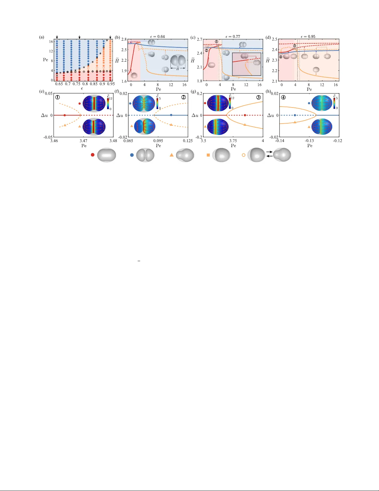
Confinemen t-Induced Symmetry Breaking of Activ e Surfaces Da Gao, 1 Alexander Mietk e, 2 , ∗ and Rui Ma 1, 3 , † 1 Dep artment of Physics, Col le ge of Physic al Scienc e and T e chnolo gy, Xiamen University, Xiamen 361005, Pe ople’s R epublic of China 2 Rudolf Peierls Centr e for The or etical Physics, Dep artment of Physics, University of Oxfor d, Parks R oad, Oxfor d OX1 3PU, Unite d Kingdom 3 F ujian Pr ovincial Key L ab or atory for Soft F unctional Materials R ese ar ch, R ese ar ch Institute for Biomimetics and Soft Matter The actom yosin cortex, a thin lay er of a cross-link ed polymer netw ork near the cell surface, generates activ e forces that are resp onsible for cell shap e changes. Man y developmen tal pro cesses that in volv e suc h cell shap e changes, most prominently embry onic cell division, are spatially confined by eggshells. T o inv estigate the p oten tial role of confinement in redirecting activ e stresses and enabling symmetry breaking phenomena during cell shape transformations, we study a hydrodynamic minimal model in whic h the cell cortex is represen ted as an active fluid surface that undergoes symmetric division in the absence of confinement. When enclosed by an ellipsoidal shell, a sp on taneous symmetry-breaking transition emerges at a critical degree of confinement, where symmetrically dividing surfaces b ecome unstable and polarized geometries app ear. W e sho w that this transition is con trolled by the tightness of the confinement and analyze the solution space of stationary surfaces to iden tify the mechanisms underlying confinement-induced symmetry breaking. Morphogenesis – the emergence of shap e in living sys- tems – relies not only on precisely orc hestrated mec hanical and bio c hemical pro cesses, but is also often constrained b y spatial confinement: Cells divide within crowded tis- sues, exp erience mechanical compression from neighbors, or are constrained by extracellular m atr ix [ 1 ]. Also the first cell divisions of most organisms that develop outside the paren t’s b ody are confined by some form of protec- tiv e lay er. In the canonical mo del organism C. ele gans , em bryonic cell division o ccurs within a rigid, ellipsoidal eggshell [2–7] . Y et the physical impact such confinemen t ma y ha ve on the cell shap e control during division remains largely unexplored. The cell cortex is a thin lay er of cross-linked actin fila- men ts and asso ciated my osin motor proteins b eneath the plasma membrane that surrounds cells. It plays a central role in cellular shap e con trol [ 8 – 11 ]. My osin generates non-equilibrium stresses that drive cortical flows and give rise to con tractile structures, such as the cytokinetic ring that pinches off a dividing cell [12–14] . During cell divi- sion, which o ccurs on minute time scales – as compared to the actom yosin turnov er that happ ens on second time scales [ 15 , 16 ] – the cortex can b e described as viscous ma- terial [ 17 ] that harb ors active stresses. Nonequilibrium hy- dro dynamic theories ha v e been systematically constructed for such systems [ 18 – 20 ]. F ocusing on the role of surface- in trinsic active stresses, these theories successfully repro- duce cortical flo ws [ 21 – 23 ] and cell shap e transformations, including cell division and p olarization [24–30]. Here, we study ho w spatial confinemen t alters the dy- namics of an active surface that undergo es cell-division- lik e shap e transformations. T o this end, w e use a minimal activ e fluid surface mo del that exhibits robust symmetric divisions in the absence of confinemen t and consider an ellipsoidal enclosure that mimics an embry onic eggshell. Using a v ariational approach to determine the nonlinear solution space of deforming activ e surface mo dels [ 31 ], w e analyze the emerging shape dynamics as the dividing surface as confinement tigh tens. W e show numerically and using analytic argumen ts that the degree of confine- men t serves as a con trol parameter to induce spontaneous symmetry breaking of a symmetrically ingressed active surface, leading to geometrically p olarized stationary and oscillatory states. Our analysis reveals that confinement stabilizes solution branches with p olar surface geometries, whic h hav e a shorter p ole-to-pole distance than symmet- rically constricted surfaces and therefore can more easily accommo date tight confinement. W e mo del the cell cortex as an axisymmetric surface parameterized by X ( u, ϕ, t ) = [ r ( u, t ) cos ϕ, r ( u, t ) sin ϕ, z ( u, t )] , (1) where u ∈ [0 , 1] and ϕ ∈ [0 , 2 π ] denote surface co ordinates. The tangent basis vectors are e i = ∂ i X with i ∈ { u, ϕ } , and the unit normal is n = ( e u × e ϕ ) / | e u × e ϕ | . A general v elo cit y field decomp oses into tangential and normal com- p onen ts, v = v ∥ + v ⊥ = v i e i + v n n , where v ∥ describ es in-plane flows and v ⊥ describ es deformations. The sur- face dynamics and lo cal center of mass v elo cit y field v are related by d X d t = v , (2) where d / d t ( · ) denotes the total time deriv ative. The ge- ometry of the surface is c haracterized by the metric tensor g ij = e i · e j and the curv ature tensor C ij = − n · ∂ i ∂ j X . The symmetric part of the velocity gradient tensor is S ij = ( ∇ i v j + ∇ j v i ) / 2 + C ij v n , and we denote its trace- less part by ˜ S ij = S ij − 1 2 S k k g ij [32]. 2 (c) (b) (a) FIG. 1. Confined symmetric divisions. (a) Surface dynam- ics (Mo vie 1) illustrating tangential surface flo ws ˜ v u = ¯ v u τ η /R 0 (red arrows) and the normalized stress-regulator concentra- tion ˜ c = c/c 0 under weak confinemen t ( ϵ = 0 . 64, where ϵ = V cell /V shell ) and weak contractilit y ( P e = 1 . 8). (b) Same confinemen t as in (a), but with increased activity ( P e = 13 . 5) (Mo vie 2). (c) Dynamics with strong confinemen t ( ϵ = 0 . 87) at the same con tractility as in (b) ( P e = 13 . 5) (Movie 3). The transparen t gra y surface illustrates the confining shell. Right panels show profiles of ˜ v u and ˜ c of the final steady states. All other parameters are listed in T able S1. The surface dynamics are gov erned by the force bal- ance equation div( T ) = − f ext , (3) where T = t ij e i ⊗ e j + t i,n e i ⊗ n denotes the total surface stress tensor and f ext = f ext i e i + f ext n n the external force densit y . The surface divergence op erator is defined as div ( · ) = e i · ∂ i ( · ). F ollo wing previous w ork on minimal mo dels of activ e self-organized surfaces [ 31 , 33 ], we con- sider a surface stress tensor that comprises of b oth equi- librium and dissipative contributions. The former read t e ij = κ 2 C k k  C k k g ij − 2 C ij  (4) t e i,n = κ ∇ i C k k (5) and follow from a Helfrich bending energy [ 32 , 34 , 35 ]. The dissipative tension tensor is c hosen as [30, 31, 33] t d ij = 2 η s ˜ S ij + η b div( v ) g ij + ξ ∆ µ g ij , (6) where η s and η b denote the surface shear and bulk vis- cosities, respectively . The last term describ es an isotropic activ e tension with con tractility ξ and chemical p oten tial difference ∆ µ . The in-plane comp onen ts of the external force den- sit y f ext are given b y f ext j = − Γ v j , (7) where Γ denotes an effective friction co efficien t. In this w ork, we consider an external normal forces giv en by f ext n = p + f c n . (8) In addition to a pressure p difference across the surface that enforces conserv ation of the enclosed v olume, we include in this work a force densit y f c n in Eq. (8) that imp oses a spatial confinemen t of the surface into a prolate ellipsoidal volume V shell . W e implement this force using a p oten tial P ext = P 0 exp  1 w p 2  z 2 a 2 + r 2 b 2 − 1  , (9) whic h is constant on ellipsoidal surfaces with a and b b eing the semi-ma jor and minor axes ( a ≥ b ), and V shell = (4 π / 3) ab 2 . The confining force is then given b y f c n = − ( ∇ P ext ) · n . (10) W e choose w p small enough that the confining p oten tial exerts a significan t force only near the b oundary , and P 0 large enough to ensure that the surface shap e remains within the confinement. Balancing n umerical stabilit y and ph ysical fidelity , we use w p = 0 . 14 and P 0 = 0 . 9 κ/R 2 0 . Activ e tension in Eq. (6) is regulated by the concentra- tion field c of a stress regulator as [37, 38] ξ ∆ µ = ( ξ ∆ µ ) 0 H + ( c ) = ( ξ ∆ µ ) 0 c 2 c 2 + c 2 s , (11) where c s denotes the saturation concen tration. The dy- namics of the regulator concentration are go verned by a con tinuit y equation d c d t = − c div ( v ) + D ∆ Γ c − k ( c − ˆ c 0 ) , (12) where terms on the right capture lo cal dilation and com- pression effects, in-plane diffusion characterized by a diffusion constant D with Laplace–Beltrami op erator ∆ Γ c = ∇ i ∇ i c , and the last term describ es exchange with the surrounding in terms of an off-rate k and a steady- state concentration ˆ c 0 . F or uniform ˆ c 0 this mo del predicts – b ey ond a critical contractilit y ξ – a sp on taneous surface p olarization in which stress regulator accumulates at one p ole [ 30 , 31 , 33 ]. T o capture the mechano-c hemical fea- tures of a division-like dynamics instead, we therefore prescrib e ˆ c 0 ( u ) as a Gaussian function p eak ed at the surface midplane: ˆ c 0 ( u ) = c 0 " 1 + ∆ c exp −  u − 1 2  2 w 2 !# , (∆ c > 0) . (13) This functional form parametrizes upstream regulatory mec hanisms that preferentially recruits stress regulator to the equatorial region, consistent with exp erimen tal 3 Steady state establishment Symmetry br eaking (b) (a) (d) (e) (f) (g) (c) FIG. 2. Dynamics of confinement-induced symmetry breaking. (a) Representativ e evolution of a symmetry-breaking ev ent showing stress regulator concentration ˜ c = c/c 0 (color scale) and tangen tial surface flows ˜ v u (red arrows). (b) W eakly p olarized steady state in which the contractile ring stabilizes at an intermediate position b et ween the p ole and the equatorial plane ( P e = 3 . 83, Movie 4). (c) Time evolution of the lo cation of maximal stress regulator concentration u max ( t ). Orange triangle depicts the time corresp onding to snapshot in (b). (d) One cycle of a persistent oscillatory state of asymmetric contractile ring formation and slipping ( P e = 4 . 5, Movie 5). (e) T emp oral evolution of stress regulator concentration ˜ c at p ole u = 0 (top) and u max (b ottom) for dynamics shown in (d). (f ) One damp ed oscillation cycle ( i − iii ) follow ed by the final steady state ( iv ). ( P e = 6 . 3, Movie 6). Black arro ws indicate magnitude of the normal velocity ˜ v n at the p ole ( u = 0). (g) T emp oral evolution of ˜ c (top) and the normal velocity ˜ v n (b ottom) at u = 0 asso ciated (f ). Data sho wn uses confinement magnitude ϵ = 0 . 87, all other parameters are listed in T able S1 [36]. observ ations of spindle–cortex interactions [ 39 – 41 ]. Pa- rameters ∆ c and w in Eq. (13) set the regulation strength and width of the regulated region, resp ectiv ely . F ollowing [ 31 ], we conv ert force balance and contin uity Eqs. (3) and (12) into a boundary v alue problem (BVP) that can b e solved iteratively to determine the time evolu- tion of the surface shap e X , the v elo cit y field v , and the concen tration field c [ 36 ]. The dynamics are initialized with a homogeneous concen tration c = c 0 , a v anishing flo w field v = 0, and a surface shap e X that is station- ary in the absence of contractilit y ( ξ ∆ µ = 0) for the giv en confinement. Characteristic time and length scales are defined as τ η = η b R 2 0 /κ and R 0 , resp ectiv ely , where the cell volume is V cell = 4 π R 3 0 / 3. The magnitude of activ e con tractility is characterized b y the P´ eclet num- b er P e = ( ξ ∆ µ ) 0 H + ( c 0 ) R 2 0 / ( D η b ). A key parameter in our analysis is the degree of confinement, ϵ = V cell /V shell , whic h ranges from 0 (no confinemen t, V shell → ∞ ) to 1 for maximally tight confinement. W e first demonstrate several representativ e dynamical b eha viors asso ciated with symmetric division. Under rela- tiv ely weak confinement ( ϵ = 0 . 64) and weak contractilit y ( P e = 1 . 8), the stress regulator accumulates at the equa- tor and forms a contractile ring that driv es surface flo ws from the p oles to ward the equator. As a result, the sur- face even tually adopts a partially ingressed steady state shap e (Fig. 1a). As con tractility is increased, surface flo ws gain magnitude, and the stress regulator b ecomes even more strongly enriched at the equator. Consequen tly , final steady states exhibit more and more pronounced constric- tions. At strong contractilit y ( P e = 13 . 5), the final steady state surface is almost completely ingressed, resulting in a V-shap ed geometry near the equator (Fig. 1b). Tighten- ing the confinement ( ϵ = 0 . 87) still allows for ingression, but daughter cells remain very close throughout the divi- sion pro cess, and hardly an y space is left betw een them at the final steady state (Fig. 1c). Such dynamics and cell morphology closely resemble that of the C. ele gans zygote during its first embry onic division [42]. A t intermediate P ´ eclet num b ers, confinement induces a sp on taneous symmetry breaking: the contractile ring ceases to constrict symmetrically and instead slips tow ard one of the p oles (Fig. 2a). Depending on the v alue of P e , three distinct regimes emerge from this ring slip. W e char- acterize these regimes by trac king the position u ∈ [0 , 1] of the concentration maximum o ver time and denote the re- sulting function b y u max ( t ). F or increased P e , the slipp ed ring remains at a p osition b et ween a p ole and the equator, leading to a stationary , asymmetrically ingressed p ear- shap ed geometry (Fig. 2b,c, P e = 3 . 83). Increasing P e further, the ring fully slips and a cluster of high stress regulator concentration remains at the p ole. Two distinct b eha viors w ere then observed: (1) Persistent oscil lations , where the p olar cluster dissolves and a new ring reassem- bles at an intermediate p osition b efore migrating pole- w ard again to rep eat the cycle (Fig. 2d,e, P e = 4 . 5); and (2) Damp e d oscil lations , where the p ole to wards whic h the ring slipp ed exhibits damp ed shape oscillations and even- tually remains flattened due to locally increased stress regulator concentration (Fig. 2f,g, Pe = 6 . 3). A general ov erview of the parameter regions that give rise to these dynamical regimes is pro vided in the phase 4 (a) (b) (c) (d) 1 2 4 3 (e) (f) (g) (h) 1 2 3 4 FIG. 3. Phase diagram and stationary shap e spaces of confined active surfaces. (a) Phase diagram for the degree of confinemen t ϵ = V cell /V shell and the P´ eclet num b er P e = ( ξ ∆ µ ) 0 H + ( c 0 ) R 2 0 / ( D η b ) quantifying the strength of activity . Symbols depict numerical simulations (representativ e shap es at the b ottom). Background shades indicate surface geometry: symmetric w eakly (red) and strongly (blue) ingressed, and polarized (orange). Parameters used in Fig. 1 are indicated b y × . T urning points of solution branc hes formed by symmetric, weakly ingressed surfaces (red lines in panels b–d) are denoted by ∗ . Numerically determined pitchfork bifurcation p oin ts (+) agree well with critical p oin ts predicted from semi-analytical arguments ( ◦ , see Eq. (14) and Fig. S3 in [ 36 ]). (b–d) Pole-to-pole distance ˜ H = H/R 0 along stationary solution branches for different confinement degrees (black arrows in a). Solid (dashed) lines indicate stable (unstable) solutions and color shading as in panel a. T ransitions to p olarized surfaces (red to orange) and to strongly ingressed symmetric surfaces (red/orange to blue) in the phase diagram are determined by bifurcations and turning p oin ts, respectively , along symmetric, weakly ingressed surface branc hes (red lines). Oscillations o ccur for Pe b ound b y dashed lines in (c) and (d). Polar surfaces generally exhibit shorter p ole-to-pole distances and can therefore more easily accommo date tight confinement. (e–h) Solution branches of weakly (e) and strongly (f ) ingressed symmetric surfaces connect to corresp onding p olar surfaces via sub critical bifurcations (e,f ) that b ecome supercritical (g,h) when tigh tening the confinement. ∆ u = u max − 1 2 quan tifies the asymmetry of the contractile ring p osition and scales as | P e − Pe ∗ | 1 / 2 in the vicinity of the bifurcation p oin t (see Fig. S4 in [36]). diagram Fig. 3(a), whic h is spanned b y the confinemen t degree ϵ and the P ´ eclet num b er P e . A t weak confinement ( ϵ ≲ 0 . 7), surfaces relax to symmetrically ingressed sta- tionary geometries: a partially ingressed shap e at low P e (Fig. 3a, red shade) and a completely ingressed morphol- ogy at high P e (Fig. 3a, blue shade). As confinement b ecomes tighter ( ϵ ≳ 0 . 7), stationary surfaces with p olar symmetry emerge (orange shade in Fig. 3a; see Fig. 2b, d, f for representativ e examples), amoun ting to a confinement- induced symmetry breaking and p olarization. This region spans an increasingly large range of P ´ eclet num b ers as the confinement ϵ is tightened further. T o rationalize the mec hanism of confinement-induced symmetry breaking, we directly compute stationary ge- ometries as a function of P e and systematically ev aluate their mechanical stability for v arious degrees of confine- men t. The results are depicted in Fig. 3b-d, where solid (dashed) lines indicate stable (unstable) solutions. At w eak confinement (Fig. 3b, ϵ = 0 . 64), we find for a passiv e fluid surface ( P e = 0) t wo stable stationary surface geome- tries: An exp ected prolate ellipsoidal surface that reflects the confinement geometry (red solid curve at P e = 0), and surprisingly , also an almost completely ingressed sur- face geometry (blue solid curve at P e = 0) – a solution that do es not exist in the absence of confinement [ 31 ]. Therefore, confinement can stabilize a division-lik e sur- face geometry even for passive surfaces. Increasing the P ´ eclet num b er P e , prolate surfaces ingress further and the p ole-to-pole distance H increases due to volume conser- v ation (Fig. 3b-d, solid red lines). F or weak confinemen t (Fig. 3b), this branch is stable up to a turning p oin t, where the surface reaches a maxim um p ole-to-p ole exten- sion H max ≈ 2 a , as dictated by the confining ellipsoid [see Eq. (9)]. In contrast, H decreases monotonically on the branc h of symmetric completely ingressed surfaces when increasing P e (Fig. 3b-d, solid blue lines). Not only in the absence of confinement [ 31 ], but also for finite v ery weak confinemen t ( ϵ ≲ 0 . 4), weakly and strongly ingressed branc hes are connected b y a Gibbs lo op and fully ingressed geometries are only stable for P e > 0 (see Fig. S2 in [ 36 ]). As ϵ increases and confinement tigh t- ens, this Gibbs loop deforms, and fully ingressed, stable geometries can also exist for Pe = 0. Bey ond these symmetric regimes, we identify a third 5 set of solution branches along which surface geometries obtain a polar asymmetry (Fig. 3b-d, orange lines). These branc hes encompass t wo kinds of scenarios. One is c har- acterized by the displacement of the contractile ring to an in termediate p osition b et ween the p ole and the equato- rial plane, which we refer to as we akly p olarize d surfac es . Dep ending on the magnitude of contractile tension, the resulting geometry is either p ear-shaped or is c haracter- ized by an asymmetrically positioned, strongly ingressed furro w (inset shap es in Fig. 3b sho w representativ e ex- amples). The second type of p olar surface geometry – str ongly p olarize d surfac es —app ears when the contractile ring has fully slipp ed, while a cluster of high stress regula- tors remains at a significantly flattened p ole. Ov erall, we find that weakly p olarized surfaces are only stable in v ery narro w P´ eclet n umber interv als, while strongly p olarized surfaces are stable for a broader range of Pe (Fig. 3a, see orange triangles and squares). Tigh tening the confinement leads to significant changes in the stationary shap e space (Fig. 3c, ϵ = 0 . 77). In con trast to the weak er confinement (Fig. 3b), the sta- ble part of the branch of symmetric weakly constricted surfaces (red solid line) now b ecomes unstable before it reac hes the turning p oin t imp osed b y the confinement (Fig. 3c, inset). A t the bifurcation, a w eakly p olarized branc h emerges via a subcritical pitchfork bifurcation (Fig. 3e). The pole-to-p ole distance H de cr e ases along this new branch, and surfaces become stable within a narro w range of P ´ eclet num b ers (Fig. 3c, inset). This marks the initial app earance of stable surface geometries with p olar asymmetry in the phase diagram (Fig. 3a) and suggests a mec hanism for confinement-induced symmetry breaking: Geometric polarization of weakly constricted surfaces reduces their p ole-to-p ole distance, making it easier to adapt to tight confinement and leading to the destabilization of symmetric surfaces with larger p ole- to-p ole distances. At high P e , stable strongly polarized surface geometries generally app ear on this branc h for all magnitudes of confinement (Fig. 3b-d, solid orange lines), corresp onding to final states of the damp ed oscil- lations shown in Fig. 2f. F or P e b ey ond, but close to, the symmetry breaking transition (P´ eclet n umber inter- v als b ounded by blac k dashed lines in Fig. 3c,d), neither w eakly nor strongly p olarized geometries are stable. As a result, p ersisten t oscillations b et w een these tw o states (Fig. 2d) emerge from a transition that exhibits signatures of a Hopf bifurcation [ 36 ], i.e. an oscillation frequency that scales as ω ∝ | Pe − P e ∗ | and an oscillation amplitude that scales as A ∝ | Pe − Pe ∗ | 1 / 2 (see Fig. S5 in [36]). F or sufficien tly tight confinement, a new bifurcation also app ears on the branc h of fully ingressed surfaces (Fig. 3 c-d , blue lines). Analyzing first the case ϵ = 0 . 77 (Fig. 3c), a sub critical pitchfork bifurcation appears at small but finite Pe (Fig. 3f ) and gives rise to an unstable branch of w eakly p olarized, strongly ingressed surface geometries (dashed orange lines). F or v ery tight confinemen t (Fig. 3d, ϵ = 0 . 95), the tw o bifurcations illustrated in Fig. 3e (w eak ingression) and Fig. 3f (strong ingression) undergo a criticality transition from sub critical to sup ercritical (Fig. 3g,h). The bifurcation sho wn in Fig. 3h implies for fully ingressed surface geometries that, under extensile activ e tension ξ < 0 ⇒ P e < 0, symmetric surfaces can b ecome unstable and give wa y to stable surfaces with p olar asymmetry (Fig. 3h). The loss of stability of symmetric surfaces at bifurca- tions (Fig. 3e and g), as well as the presence of stable w eakly polarized surface geometries at or nearb y these bifurcations, delineates the b oundary b et w een symmetric (blue) and p olarized (orange) surface geometries in Fig. 3a. Notably , the critical P ´ eclet num b er P e ∗ asso ciated with this symmetry-breaking transition seems insensitiv e to the degree of confinemen t ϵ . T o rationalize this, w e ana- lyze steady-state concentration and flow profiles along the branc h of w eakly ingressed symmetric surfaces (red lines). Stress-regulator concentration is strongly lo calized at the equatorial plane ( u = 1 / 2), where it reaches its maxim um v alue c max , while the meridional flo w v u exhibits a signif- ican t gradien t ∂ u v u . A linear stability analysis yields a semi-analytical expression for the effective growth rate λ of surface p erturbations [36], λ ≈ − D q 2 min − k − ∂ u v u + ξ ∆ µ η b H ′ + ( c max ) c max , (14) where q min is a fitting parameter that denotes the min- im um wa ven umber to b e considered for linear stability analysis. While diffusive damping ( − D q 2 min ) and degra- dation ( − k ) stabilize a symmetric surface, the active stress and flows promote shap e p olarization. V alues P e ∗ predicted with Eq. (14) agree well with numerically de- termined bifurcation p oin ts (compare black + and ◦ in Fig. 3a). This analysis also reveals that the instabilit y is primarily driven by compressiv e flow gradients ( − ∂ u v u ) at the equator as con tractility P e increases [ 36 ]. The turning p oin ts of the symmetric, weakly ingressed branch delineate the phase b oundary b etw een the p olarized (or- ange) and symmetric division (blue) regimes in the phase space (Fig. 3a). F or v alues of Pe b ey ond these turn- ing p oin ts, the stationary shap e space no longer holds stationary solutions of symmetric, w eakly ingressed sur- faces. Instead, a sufficiently large active con tractility (i.e. large P e ) suppresses the symmetry-breaking instability and drives surfaces again to ward a symmetric, completely ingressed geometry . In this Letter, w e hav e demonstrated that spatial con- finemen t can destabilize symmetrically constricting active fluid surfaces and giv e rise to a sp on taneously emerging p o- lar asymmetry . Mathematically , this symmetry-breaking arises from confinement-enhanced pitchfork bifurcations in the stationary shape space. Physically , it arises b ecause constricted surfaces with p olar asymmetry fit more easily in to tight confinement than symmetric ones. 6 Asymmetric division is a hallmark of early C. ele gans dev elopment and is linked to a pre-established bio c hemi- cal p olarit y [ 43 , 44 ]. The degree of confinement during this division is appro ximately ϵ = 0 . 85 [ 24 , 45 , 46 ], a v alue that resides within the p olarized regime of our sta- tionary shape space for a broad range of P e (Fig. 3a, orange shaded region). Our results suggest that spatial confinemen t provided by the eggshell could play a critical role in reinforcing this asymmetry . This is also consis- ten t with exp erimen tal observ ations of more symmetric divisions when the eggshell surrounding C. ele gans em- bry os is remov ed [ 47 ]. Our analysis also indicates that asymmetric, strongly ingressed surfaces are mec hanically unstable under con tractile active tension, which suggests that additional mechanical factors are required to sus- tain complete asymmetric divisions. Candidates for this missing ingredient are anisotropic active tension [ 14 , 48 ] and sp on taneous curv ature [ 41 ]. Importantly , cells that divide within biological tissues also exp erience effective confinemen t due to surrounding cells and the extracellular matrix. Motiv ated by these observ ations, it will b e in ter- esting to inv estigate how bio c hemical p olarit y cues and confinemen t with alternative geometric and mechanical prop erties influence the shap e dynamics and robustness of cell division. W e ackno wledge financial supp ort from the National Natural Science F oundation of China under Grant No. 12474199 and the F undamental Researc h F unds for Cen- tral Universities of China under Grant No. 20720240144, as well as from the 111 pro ject B16029. Numerical approac h The numerical approaches used in this w ork are describ ed in detail in ref. [ 31 ] and the corresp onding co de is av ailable on GitHub as referenced therein. T o be self-contained, we pro vide in the following a brief summary . P arameterized axisymmetric surfaces W e consider deforming axisymmetric surfaces parameterized as X ( u, ϕ, t ) =  r ( u, t ) cos ϕ, r ( u, t ) sin ϕ, z ( u, t )  , (S1) where r ( u, t ) and z ( u, t ) denote the time-dep enden t meridional profiles of the surface co ordinates, and we refer to the time-indep enden t parameterization u ∈ [0 , 1] and ϕ ∈ [0 , 2 π ] as mesh co ordinates (Fig. S1). T angent vectors e i = ∂ i X and surface normal n = e u × e ϕ / | e u × e ϕ | are given by e u = h ¯ e u = h   cos ψ cos ϕ cos ψ sin ϕ − sin ψ   e ϕ = r ¯ e ϕ = r   − sin ϕ cos ϕ 0   n =   sin ψ cos ϕ sin ψ sin ϕ cos ψ   , (S2) where h = p ( r ′ ) 2 + ( z ′ ) 2 is a scaling factor ( ′ denotes deriv ative w.r.t. u ), ψ is the tangent angle, and ¯ e u and ¯ e ϕ are normalized tangen t vectors. Scaling factor h and tangen t angle ψ and scaling factor are related to surface coordinates by r ′ = h cos ψ , (S3) z ′ = − h sin ψ , (S4) where primes denote deriv ativ es with resp ect to u . Metric tensor g ij = ( ∂ i X ) · ( ∂ j X ) and area elemen t dA = p det( g ij ) ds 1 ds 2 read g ij =  h 2 0 0 r 2  (S5) dA = hrdudϕ. (S6) Curv ature tensor comp onen ts C j i = − g j k n · ∇ i ∇ k X are given by C j i =  ψ ′ /h 0 0 sin ψ/r  , (S7) where the diagonal elemen ts corresp ond to the t wo principal curv atures of the surface. 7 Constrained dissipation functional W e solve the force balance Eq. (3) (main text) and evolv e the surface according to Eq. (2) using a dissipation functional formulation (see [31] for details). This functional assumes the form R = 2 π Z 1 0 " ∂ t f κ + f κ ∂ t ( r h ) r h − r p ∆ µ − f ext c · v + 1 2 ( S 1 + S 2 + S 3 ) + 1 2 Γ  ¯ v 2 u + ¯ v 2 ϕ  # r h du + 2 π Z 1 0 du ∂ t [ α ( r ′ − h cos ψ ) + β ( z ′ + h sin ψ ) + ζ h ′ ] , (S8) where ∂ t f κ = ∂ f κ ∂ r ∂ t r + ∂ f κ ∂ ψ ∂ t ψ + ∂ f κ ∂ ψ ′ ∂ t ψ ′ + ∂ f κ ∂ h ∂ t h (S9) describ es contributions from b ending energy density f κ = 1 2 κ  ψ ′ h + sin ψ r  2 , (S10) and the terms S 1 = η b  ¯ S uu + ¯ S ϕϕ  2 (S11) S 2 = η s h  ¯ S uu − ¯ S ϕϕ  2 +  2 ¯ S uϕ  2 i (S12) S 3 = 1 Λ  r p + ξ  ¯ S uu + ¯ S ϕϕ  2 (S13) con tain contributions from the strain rate tensor components ¯ S uu = 1 h ¯ v ′ u + ψ ′ h v n (S14) ¯ S ϕϕ = cos ψ r ¯ v u + sin ψ r v n (S15) ¯ S uϕ = 1 2  ¯ v ′ ϕ h − cos ψ r ¯ v ϕ  . (S16) Sp ecific to the present w ork is the external force f ext c in Eq. (S8), whic h is giv en by f ext e = ( p + f n c ) n , (S17) where the pressure difference p acts as a Lagrange m ultiplier that enforces the conserv ation of the enclosed v olume V cell the second term is given b y f n c = −  ∂ P ext ∂ r sin ψ + ∂ P ext ∂ z cos ψ  , (S18) for the confinement p oten tial P ext written in Eq. (9) (main text). The second line in Eq. (S8) imp oses the geometric relationships giv en by Eqs. (S3) and (S4) with Lagrange m ultipliers α and β . The Lagrange multiplier ζ enforces a scaling Lagrangian–Eulerian (SLE) parameterization defined by the condition h ′ = 0 , (S19) a gauge c hoice for the paramterization that can alw ays b e made [ 31 ]. With this choice, the scaling factor b ecomes spatially uniform, h ( u, t ) = h ( t ) and only dep ends on time. Consequen tly , the map b et ween mesh coordinate u and 8 ph ysical arc length s along the meridional contour is simply s = h ( t ) u. (S20) Accordingly , h ( t ) coincides with the total arclength L of the meridional outline (Fig. S1). In ref. [31], w e hav e shown that δ R δ Φ = 0 . (S21) with R given in Eq. (S8) and Φ ∈  v u , v ϕ , ∂ t r , ∂ t z , ∂ t h, ∂ t ψ , ∂ t α, , ∂ t β , ∂ t ζ  , yields a system of equations that is equiv alent to the force and momen t balance equations of the active fluid surface. Boundary terms of this v ariation provide b oundary conditions (see T ab. S3) for solving the resulting b oundary v alue problem. Boundary v alue problems F rom the pro cedure describ ed ab o ve, we find dynamic equations for ∂ t r , ∂ t z , and ∂ t ψ . Depending on the need for dynamic simulations or the computation of numerically exact stationary surfaces, we consider tw o strategies: • T o p erform dynamic simulations, w e connect tw o time steps that are separated by ∆ t b y setting the time deriv atives to ∂ t r = r ( u, t ) − r ( u, t − ∆ t ) ∆ t ∂ t z = z ( u, t ) − z ( u, t − ∆ t ) ∆ t ∂ t ψ = ψ ( u, t ) − ψ ( u, t − ∆ t ) ∆ t , (S22) and using r ( u, t − ∆ t ) , z ( u, t − ∆ t ) , ψ ( u, t − ∆ t ) from the previous time-step. This represen ts a robust implicit in tegration the dynamic equations. Solutions [ r ( u, t ) , z ( u, t ) , ψ ( u, t ) , v u , v ϕ ] deriv ed from this b oundary v alue problem directly corresp ond to the surface geometries and flows at the next time p oin t. T o enforce volume conserv ation, we in tro duce the auxiliary volume function V ( u ), which satisfies V ′ = π r 2 h sin ψ , (S23) together with the b oundary conditions V (0) = 0 , V (1) = V cell = 4 π 3 R 3 0 . (S24) W e solve the b oundary v alue problem arising at every time step using standard solvers as implemented in MA TLAB [49]. The parameter v alues used in the sim ulations are listed in T ab. S1. • T o compute steady-state solutions directly , we imp ose ∂ t r = 0 , ∂ t z = v 0 , ∂ t ψ = 0 , (S25) in the system of equations arising from the v ariation Eq. (S21), where v 0 is an additional parameter representing a p ossible translational velocity of the surface along the symmetry axis. In the absence of confinement, v 0 is an unkno wn that m ust b e determined as part of the b oundary v alue problem. An additional b oundary condition 9 z (0) + z (1) = 0 is used to fix the reference frame that co-mov es with the surface [ 30 ]. In the presence of confinemen t, steady state requires v 0 = 0. W e therefore in tro duce an additional b oundary condition z (0) + z (1) = ∆ z , (S26) and tune the parameter ∆ z suc h that the solution satisfies v 0 = 0. Steady-state solutions are obtained iteratively by gradually increasing the activit y parameter ξ (or equiv alently the P´ eclet n umber P e ), using the solution at the previous parameter v alue as the initial guess. In the presence of degeneracies, where multiple steady-state solutions exist for a given P e , contin uation through turning p oin ts is ac hieved b y instead incrementing the p ole-to-pole distance H = z (0) − z (1) , (S27) while treating the con tractility ξ as an additional unknown parameter. Initial conditions The dynamic simulations are initialized from a steady state in the absence of contractilit y ( P e = 0). T o obtain this reference state, we b egin with a very weak confinement in a prolate geometry , for which a spherical surface with a uniform distribution of stress regulators constitutes a steady-state solution. W e then iteratively decrease the confinemen t dimensions a and b , while k eeping their ratio fixed at a/b = 1 . 3. This yields deformed, but homogeneous steady-state solutions at progressively stronger confinemen t that serve as initial conditions for simulations in whic h activit y is turned on. Numerical test of stabilit y of stationary solutions Once stationary branches are identified, w e test the stability of solutions along these branches b y applying a small p erturbation δ c to the steady concentration field c 0 , i.e. w e use c ( u, t = 0) = c 0 + δ c as an initial condition in a dynamic simulation. The distance || f − f 0 || := || r ( u, t ) − r 0 ( u ) || 2 + || z ( u, t ) − r 0 ( u ) || 2 + || c ( u, t ) − c 0 ( u ) || 2 is used as a measure of the deviation of the dynamic solution f from the steady stationary solution f 0 . Here, || · || 2 denotes the L 2 norm on u ∈ [0 , 1] (see Fig. S6). Linear stabilit y analysis of nonlinear steady states Here, we p erform a linear stability analysis of weakly ingressed steady states (see red curv es in Fig. 3a,b,c of the main text). This analysis provides an indep enden t and complementary criterion for assessing the stability of nonequilibrium steady states, alongside direct numerical in tegration of the full dynamical equations with p erturbed steady state taken as the initial condition (see Sec. ). The final result is the semi-analytical expression giv en in Eq. (14) (main text) for the critical conditions at which spontaneous symmetry breaking occurs. Axial parameterization F or this analysis, we in tro duce an axial parameterization X ( z , ϕ, t ) =  r ( z, t ) cos ϕ, r ( z , t ) sin ϕ, z  , (S28) whic h enco des the surface geometry by a single function r ( z , t ). While this parameterization is not suitable to describ e arbitrary axisymmetric surfaces for which r ( z , t ) can b e multi-v alued, it is sufficien t for a linear analysis near w eakly ingressed shap es that are describ ed by a well-defined single-v alued radial function. 10 F or the parameterization Eq. (S28), the tangent basis and normal v ectors are E z = p 1 + ( r ′ ) 2 ¯ E z =   r ′ cos ϕ r ′ sin ϕ 1   E ϕ = r ¯ E ϕ =   − r sin ϕ r cos ϕ 0   N = 1 p 1 + ( r ′ ) 2   − cos ϕ − sin ϕ r ′   . (S29) where ¯ E i depict normalized tangent vectors. The non-v anishing metric tensor and curv ature tensor comp onen ts are g z z = p 1 + ( r ′ ) 2 g ϕϕ = r 2 . (S30) and C z z = − r ′′ (1 + r ′ 2 ) 3 / 2 C ϕ ϕ = 1 r √ 1 + r ′ 2 , (S31) resp ectiv ely . Here and in the following deriv ation, primes ′ denote deriv atives with resp ect to z , and dots ˙ denotes time deriv atives. Kinematic equations The center of mass flow v is decomp osed as v ( z , ϕ, t ) = v ( z , t ) ¯ E z + v n ( z , t ) n , (S32) where v ( z , t ) is the tangential v elo cit y along the meridional direction, and v n ( z , t ) is the normal v elo cit y . The surface dynamics reads d d t [ X ( z , ϕ, t )] = v ( z, ϕ, t ) , (S33) where the material deriv ative of a function f ( z , t ) is defined as d f d t = ˙ f + q z f ′ . (S34) Here, q z denotes the co ordinate flow associated with the parameterization Eq. (S28). F rom Eq. (S33), we find v n ( z , t ) = ˙ r p 1 + ( r ′ ) 2 , (S35) while the co ordinate flow is given by q z = − ˙ r r ′ 1 + ( r ′ ) 2 + v p 1 + ( r ′ ) 2 . (S36) Mapping b et ween the { z , ϕ } and { u, ϕ } parameterizations Using the geometric relations ds = h du = dr cos ψ = − dz sin ψ , (S37) as well as cos[ ψ ( u, t )] = − ∂ z r p 1 + ( ∂ z r ) 2 , sin[ ψ ( u, t )] = 1 p 1 + ( ∂ z r ) 2 , (S38) 11 together with the identit y ¯ E z = − ¯ e u , we establish the mapping betw een fields defined in the { z , ϕ } and { u, ϕ } parameterizations. Specifically , we obtain r ( z, t ) = r ( u, t ) , ∂ z r ( z, t ) = ∂ u r ( u, t ) ∂ u z ( u, t ) = − cot ψ ( u, t ) , (S39) v ( z , t ) = − ¯ v u ( u, t ) , ∂ z v ( z , t ) = − ∂ u ¯ v u ( u, t ) ∂ u z ( u, t ) = 1 sin ψ ( u, t ) ∂ u ¯ v u ( u, t ) h ( u, t ) , (S40) c ( z , t ) = c ( u, t ) , ∂ z c ( z , t ) = ∂ u c ( u, t ) ∂ u z ( u, t ) = − 1 sin ψ ( u, t ) ∂ u c ( u, t ) h ( u, t ) . (S41) When conv erting a function f ( z , t ) to its representation f ( u, t ), the corresp onding co ordinate u is obtained b y in verting the relation z = z ( u, t ). Finally , with the ab o v e identities, it’s easy to verify that the co ordinate flow Eq. (S36) is equiv alent to the co ordinate flo w equation [31] q u = v u + h − 1 (sin ψ∂ t z − cos ψ ∂ t r ) (S42) for the { u, ϕ } parameterization. F orce balance equations The force balance equations in the { z , ϕ } parameterization can b e deriv ed by constructing a Ra yleigh dissipation functional analogous to that used in the { u, ϕ } co ordinate system, and subsequen tly taking v ariations with resp ect to ∂ t r ( z , t ) and v ( z , t ). F or brevity , w e omit the in termediate steps of this deriv ation and present only the resulting equations b elo w. The normal force balance equation reads in axial co ordinates D 1 ˙ r = 1 2 κ (  1 + ( r ′ ) 2  3  1 + 2( r ′ ) 2  − r r ′′  1 − 3( r ′ ) 4 − 2( r ′ ) 6  − r 2  1 + ( r ′ ) 2   3( r ′′ ) 2  1 − 4( r ′ ) 2  + 4 r ′ r ′′′  1 + ( r ′ ) 2  + r 3  5( r ′′ ) 3 (1 − 6( r ′ ) 2 ) + 20 r ′ r ′′ r ′′′ (1 + ( r ′ ) 2 ) − 2 r ′′′′ (1 + ( r ′ ) 2 ) 2  ) + η b ( − r ( v r ) ′  1 + ( r ′ ) 2  5 / 2  1 + ( r ′ ) 2 − r r ′′  ) + η s ( − r ( v r ′ − r v ′ ) h 1 + ( r ′ ) 2 i 5 / 2 h 1 + ( r ′ ) 2 + r r ′′ i ) + ξ H + ( c )  1 + ( r ′ ) 2  3 n r 3 r ′′ − r 2  1 + ( r ′ ) 2  o + r 3  1 + ( r ′ ) 2  9 / 2 f ext n , (S43) where D 1 = r  1 + ( r ′ ) 2  ( ( η s + η b )  (1 + ( r ′ ) 2 ) 2 + r 2 ( r ′′ ) 2  + 2( η s − η b ) r  1 + ( r ′ ) 2  r ′′ ) . (S44) 12 The meridional force balance equation reads in axial co ordinates: D 2 ˙ r ′ = η s ( − ˙ r r ′  1 + ( r ′ ) 2  5 / 2 − v ( r ′ ) 2  1 + ( r ′ ) 2  3 + v ′ r r ′  1 + ( r ′ ) 2  3 − v rr ′′  1 + ( r ′ ) 2  2 + v ′′ r 2  1 + ( r ′ ) 2  3 − v ′ r 2 r ′ r ′′  1 + ( r ′ ) 2  2 − ˙ r r 2 r ′′′  1 + ( r ′ ) 2  3 / 2 + 4 ˙ r r 2 r ′ ( r ′′ ) 2 p 1 + ( r ′ ) 2 ) + η b ( − ˙ r r ′  1 + ( r ′ ) 2  5 / 2 − v ( r ′ ) 2  1 + ( r ′ ) 2  3 + v ′ r r ′  1 + ( r ′ ) 2  3 + v rr ′′  1 + ( r ′ ) 2  2 + v ′′ r 2  1 + ( r ′ ) 2  3 − v ′ r 2 r ′ r ′′  1 + ( r ′ ) 2  2 − ˙ r r 2 r ′′′  1 + ( r ′ ) 2  3 / 2 + 4 ˙ r r 2 r ′ ( r ′′ ) 2 p 1 + ( r ′ ) 2 − 2 ˙ r rr ′ r ′′  1 + ( r ′ ) 2  3 / 2 ) + ξ r 2 c ′ g ′ ( c )  1 + ( r ′ ) 2  7 / 2 − Γ v r 2  1 + ( r ′ ) 2  4 , (S45) where D 2 = r  1 + ( r ′ ) 2  3 / 2 ( η s h 1 + ( r ′ ) 2 + r r ′′ i + η b h r r ′′ − [1 + ( r ′ ) 2 ] i ) . (S46) Dynamic equation of the concen tration field Using the definition of the material deriv ativ e in Eqs. (S34) and (S36) , the dynamics Eq. (12) go verning the evolution of the concentration field c in the { z , ϕ } parameterization reads ˙ c = ˙ r  1 + ( r ′ ) 2  ( r r ′ c ′ − c ) + rr ′′ c r [1 + ( r ′ ) 2 ] 2 + D − r r ′ r ′′ c ′ + ( r ′ c ′ + r c ′′ )  1 + ( r ′ ) 2  r [1 + ( r ′ ) 2 ] 2 − k ( c − ˆ c 0 ) − ( v cr ) ′ r p 1 + ( r ′ ) 2 . (S47) Linearized equations W e assume that the force balance equations Eqs. (S43) and (S45) , together with the concentration dynamics Eq. (S47) , admit a steady-state solution { r ss ( z ) , v ss ( z ) , c ss ( z ) } . These steady states corresp ond to a symmetric, partially ingressed geometry , c haracterized by cortical flows directed from the p oles tow ard the equator and by an accum ulation of stress regulators at the equatorial region, lo cated at z = 0. Consequently , the steady-state profiles r ss ( z ) and c ss ( z ) are even functions of z , whereas the flo w profile v ss ( z ) is an odd function of z . Therefore, w e must ha ve at the symmetry plane z = 0: r ′ s 0 ≡ r ′ ss (0) = 0 , r ′′′ s 0 ≡ r ′′′ ss (0) = 0 , c ′ s 0 ≡ c ′ ss (0) = 0 , v s 0 ≡ v ss (0) = 0 , v ′′ s 0 ≡ v ′′ ss (0) = 0 . (S48) W e then in tro duce a small p erturbation around this steady state, r ( z, t ) = r ss ( z ) + ϵ δ r ( z , t ) , v ( z , t ) = v ss ( z ) + ϵ δ v ( z , t ) , c ( z , t ) = c ss ( z ) + ϵ δ c ( z , t ) , (S49) and expand the go verning equations to first order in the small parameter ϵ . The zeroth-order terms repro duce the steady-state equations, while the terms to O ( ϵ ) yield a set of linearized evolution equations for the perturbations 13 δ r ( z , t ), δ v ( z, t ), and δ c ( z , t ). The latter can b e cast into the compact form L   ˙ δ r ˙ δ c 0   = M   δ r δ c δ v   , (S50) where L and M are linear differential op erators whose co efficien ts dep end on the steady-state profiles r ss ( z ), v ss ( z ), and c ss ( z ), as well as their deriv ativ es. The linear stability of the steady state is determined by the generalized eigenv alue problem Lf n = λ n M f n , (S51) where f n are suitable eigenmo des that are unstable if their eigenv alue λ n has a p ositiv e real part. Equation (S51) is in general analytically intractable and must therefore b e solv ed numerically . T o make progress, we assume that the onset of symmetry breaking is dominated by p erturbations lo calized in the vicinit y of the equatorial plane z = 0. Accordingly , we approximate the linear differential operators L and M b y ev aluating their co efficien ts at z = 0. Exploiting the symmetry prop erties of the steady state summarized in Eq. (S49), the normal force balance equation Eq. (S43) simplifies to D 1 , 0 ˙ δ r = 1 2 κ ( r 2 s 0 (3 r s 0 r ′′ s 0 (5 r s 0 r ′′ s 0 − 2) − 1) δr ′′ − 2 r 4 s 0 δ r ′′′′ +  r 3 s 0  5( r ′′ s 0 ) 3 − 2 r ′′′′ s 0  + r s 0 r ′′ s 0 − 2  δ r ) + η b r 3 s 0 h δ v ′ ( r s 0 r ′′ s 0 − 1) + v ′ s 0 ( r s 0 δ r ′′ + r ′′ s 0 δ r ) i + η s r 3 s 0 h δ v ′ ( r s 0 r ′′ s 0 + 1) + v ′ s 0 ( r s 0 δ r ′′ + r ′′ s 0 δ r ) i + ξ r 3 s 0 h H + ( c s 0 ) ( r ′′ s 0 δ r + r s 0 δ r ′′ ) + ( r s 0 r ′′ s 0 − 1) H ′ + ( c s 0 ) δc i + f ext n r 3 s 0 δ r , (S52) where D 1 , 0 = r 2 s 0  η s ( r s 0 r ′′ s 0 + 1) 2 + η b ( r s 0 r ′′ s 0 − 1) 2  . (S53) Similarly , the meridional force balance equation Eq. (S45) reduces to D 2 , 0 ˙ δ r ′ = η s " − r ′′ s 0 δ v + v ′ s 0 δ r ′  1 − r s 0 r ′′ s 0  + r s 0 δ v ′′ # + η b " r ′′ s 0 δ v + v ′ s 0 δ r ′  1 − r s 0 r ′′ s 0  + r s 0 δ v ′′ # + ξ r s 0 H ′ + ( c s 0 ) δ c ′ − Γ r s 0 δ v (S54) where D 2 , 0 = η s − η b + ( η s + η b ) r s 0 r ′′ s 0 . (S55) Finally , the concen tration dynamics equation Eq. (S47) yields to linear order δ ˙ c + ( v ′ s 0 δ c + c s 0 δ v ′ ) = ˙ δ r  c s 0  r ′′ s 0 − 1 r s 0  + D δc ′′ − k δc (S56) W e next seek normal-mo de solutions of the form δ r ( z , t ) = δ r ( t ) e iq z , δ v ( z , t ) = δ v ( t ) e iq z , δ c ( z , t ) = δ c ( t ) e iq z , (S57) where q is the p erturbation wa ven umber. Substituting these expressions into Eqs. (S52) , (S54) , (S56) yields a closed system of linear ordinary differen tial equations for the time-dep enden t co efficien ts δ r ( t ) , δ v ( t ) and δ c ( t ) in Eqs. (S57). This system can b e written as 14  ˙ δ r ˙ δ c  =  J rr J rc J cr J cc   δ r δ c  (S58) where the comp onen ts of the 2 × 2 Jacobian matrix are given b y J rr = ξ H + ( c s 0 ) ( r ′′ s 0 − q 2 r s 0 ) 2 η b r s 0 + r 2 s 0 v ′ s 0  ( r ′′ s 0 ) 2 − q 2  + f ext n 2 η b r s 0 + κ − 2 + r s 0 n r ′′ s 0 + r s 0 h − 2 q 4 r 2 s 0 + q 2 [1 + 3 r s 0 r ′′ s 0 (2 − 5 r s 0 r ′′ s 0 )] + r s 0 [5( r ′′ s 0 ) 3 − 2 r ′′′′ s 0 ] io 4 η b r 2 s 0 , (S59) J rc = − ξ r s 0 H ′ + ( c s 0 ) 2 η b , (S60) J cr = ξ H + ( c s 0 ) c s 0 ( q 2 r s 0 − r ′′ s 0 ) 2 η b + c s 0 v ′ s 0 n 1 + r s 0  − r ′′ s 0 + r s 0 ( q 2 − ( r ′′ s 0 ) 2 )  o r s 0 − c s 0 f ext n 2 η b + κ c s 0 h 2 − q 2 r 2 s 0 + 2 q 4 r 4 s 0 − r s 0 r ′′ s 0 − 5 r 3 s 0 ( r ′′ s 0 ) 3 + 2 r 3 s 0 r (4) s 0 + 3 q 2 r 3 s 0 r ′′ s 0 (5 r s 0 r ′′ s 0 − 2) i 4 η b r 3 s 0 , (S61) J cc = − k − D q 2 + ξ c s 0 H ′ + ( c s 0 ) η b − v ′ s 0 . (S62) In Eqs. (S59)– (S62), we ha ve set η s = η b to simplify expressions. As we assume that stability is primarily gov erned by the lo cal b eha vior of the p erturbation equations in the vicinit y of the equatorial plane z = 0, corresp onding to short-wa velength modes, w e restrict our analysis to p erturbations with wa ve n umbers q larger than a minimal v alue q min . F or three representativ e v alues of con tractility , Fig. S7a shows the growth rate – defined as the real part of the largest eigenv alue of the Jacobian matrix J with comp onen ts Eqs. (S59)–(S62) – as a function of the wa v e num b er q . The v alues for c s 0 , r s 0 , and v s 0 , as well as their deriv ativ es, are taken from numerical steady state solutions along the weakly ingressed solution branch. The gro wth rate predicted by the Jacobian ab o v e decreases monotonically with increasing q . Consequently , if the gro wth rate is negative at q = q min , it remains negative for all q > q min , and the steady state is linearly stable. Con versely , if the growth rate is p ositiv e at q = q min , the steady state is unstable. W e therefore use the v alue of the largest eigenv alue of the Jacobian matrix ev aluated at q = q min as a criterion for assessing the stabilit y of the steady state. Giv en a prescrib ed v alue of q min , we can predict the critical P ´ eclet n umber P e ∗ at whic h the gro wth rate λ ( q min ) acquires a positive real part. W e treat q min as a single fitting parameter and determine its optimal v alue by minimizing the discrepancy b et w een the critical P´ eclet num b ers P e ∗ a obtained from the semi-analytical linear stability analysis and P e ∗ n determined from direct n umerical simulations across different degrees of con- finemen t. In practice, this corresp onds to minimizing the distance b et ween the p oin ts marked by ◦ and + in Fig. 3a of the main text. The growth rates computed from the semi-analytical eigen v alue analysis are shown in Fig. S7b. Notably , with q min R 0 = 11 . 5, they b ecome p ositiv e at almost the same P´ eclet num b ers at which the direct numerical simulations predict the onset of shap e instabilities, indicated by the transition from solid to dashed lines. Heuristically , we find that the growth rates predicted b y the Jacobian are w ell appro ximated b y the matrix element J cc giv en in Eq. (S62) (compare solid and dashed lines in Fig. S7a), which motiv ates the discussion of Eq. (14) in the main text. In Eq. (S62) , b oth the turnov er and diffusion terms contribute negativ ely to the gro wth rate and, therefore, act to stabilize the steady state. The steady-state concen tration of stress regulators at the equator, c s 0 , increases monotonically with the con tractility P e . Ho w ever, the term c s 0 H ′ + ( c s 0 ) exhibits a nonmonotonic dep endence on c s 0 , con tributing only a small p ositiv e correction at large c s 0 (or P e ). In contrast, the v elo cit y gradient term − v ′ s 0 pro vides a dominant positive contribution, which ultimately drives the instability . 15 Supplemen tary figures confinement T orque Force ds FIG. S1. Parameterization of the closed axisymmetric surface X ( u, ϕ, t ) . The transparent gray prolate surface represents the geometric confinement. The coordinates u = 0 and u = 1 corresp ond to the tw o poles of the surface, respectively . Under the SLE parameterization, the metric factor h ( u, t ) = h ( t ) is indep enden t of u and equal to the total arclength L . FIG. S2. Confinement-induced deformation and break-up of the Gibbs lo op in the stationary solution space. A t weak confinement ( ϵ = 0 . 38 , 0 . 45), solution branches form loops that con tinuously connects solutions corresp onding to partially ingressed and fully ingressed geometries (see [ 31 ] for corresp onding plot in the absence of any confinement). In contrast, at strong confinemen t ( ϵ = 0 . 64 , 0 . 77 , 0 . 95), these branc hes become disconnected. Insets show a zo omed-in view of the lo op structure for ϵ = 0 . 38. All other parameters are listed in T able S1. 16 FIG. S3. Critical p oin ts of weakly ingressed solution branches indicate transitions b et ween symmetric and p olarized surface shap es. At weak confinement ( ϵ = 0 . 64), solutions remain stable (solid segment of the black curv e) up to the turning p oin t ( ∗ ). As the degree of confinemen t increases, this branc h becomes unstable b efore reaching the turning p oin t, and a branch of asymmetric, partially ingressed geometries bifurcates from the symmetric branch (bifurcations indicated by +, see inset). F or P´ eclet num b ers beyond turning p oin ts, the surface undergo es a strong symmetric ingression. The lo cation of these critical points in the stationary solution space agrees well with the boundaries of regions of different dynamically emerging surface geometries depicted in the phase diagram Fig. 3a (main text). All other parameters are listed in T able S1. 1 3 2 4 (a) (b) FIG. S4. Scaling b eha vior near pitchfork bifurcations. | ∆ u | = | u max − 1 / 2 | denotes the deviation of the lo cation of the maxim um concen tration, u max , from the equatorial plane at u = 1 / 2. P e ∗ denotes critical con tractility P ´ eclet n umber of the bifurcation. (a) Scaling behavior near the bifurcation points lab eled 1 ○ and 3 ○ in Fig. 3e,g (branching of weakly ingressed p olarized surface geometries). (b) Scaling b eha v ior near the bifurcation p oin ts labeled 2 ○ and 4 ○ in Fig. 3f,h (branching of strongly ingressed p olarized surface geometries). 17 (a) (b) FIG. S5. Exemplary scaling signatures of a Hopf bifurcation at the onset of p olar shap e oscillations. (a) Oscillation frequency ˜ ω = ω τ η . (b) Oscillation amplitude ˜ A = c ( u = 0) /c 0 . Data shown uses confinement magnitude ϵ = 0 . 87 and bifurcation p oin t Pe ∗ = 4 . 24, all other parameters are listed in T able S1. (a) (b) FIG. S6. Stability testing of nonlinear stationary solutions. Stationary solutions are dynamically simulated with small concen tration p erturbations as initial conditions. W e then measure the time evolution of || f − f 0 || := || r ( u, t ) − r 0 ( u ) || 2 + || z ( u, t ) − r 0 ( u ) || 2 + || c ( u, t ) − c 0 ( u ) || 2 , where || · || 2 denotes the L 2 norm on u ∈ [0 , 1]. This test typically leads to an unambiguous con verging (a) or diverging dynamics (b), from whic h w e conclude the corresponding p oin t of the branch to b e stable or unstable, resp ectiv ely . Curves show exemplary responses from the stable and unstable parameter regions in Fig. 3b-d. 18 (a) (b) FIG. S7. Exemplary linear stabilit y analysis of nonequilibrium steady states under strong confinemen t ( ϵ = 0 . 946) . (a) Gro wth rate λ as a function of the dimensionless w av e n umber q R 0 . Only modes within the shaded region ( q > q min = 11 . 5 /R 0 ) are considered. Solid curves show the largest real part of the eigenv alues of the Jacobian matrix J , while dashed curv es sho w its J cc comp onen t. (b) Growth rates as a function of P e for differen t confinement degrees as predicted from the Jacobian with comp onen ts Eqs. (S59)–(S62). T o obtain these curves, the Jacobian is computed using the steady state v alues (and deriv atives) of the radial co ordinate r s 0 . the concentration c s 0 and flows v s 0 along the branch of symmetric, weakly ingressed surfaces (Fig. 3b–d, red curves) The change of the growth rate from negative to p ositiv e v alues indicates the onset of an instability . Solid and dashed segmen ts of the curves denote stable and unstable regimes, resp ectiv ely , as determined from direct numerical in tegration of the full dynamical equations, indicated very go od agreement with the semi-analytic stability analysis. 19 Supplemen tary tables P arameter V alue Unit κ Bending rigidity 1 κ η b Bulk viscosity 1 η b η s Shear viscosity 1 η b R 0 Spherical radius 1 R 0 τ η Time scale η b R 2 0 /κ τ η ∆ t T emp oral resolution 1/900 τ η Γ F riction 0.09 η b /R 2 0 D Diffusion constant 1 R 2 0 /τ η k T urnov er rate 45 τ − 1 η c 0 Steady state concentration 1 c 0 c s Saturation concentration 10 c 0 w Width of the regulated region 0.14 1 w p Thic kness of the confined shell 0.14 1 P 0 Strength of confinement 0.9 κ/R 2 0 T ABLE S1. P arameters used in closed active fluid surface examples shown in Figs. 1–3. The characteristic time in these sim ulations is defined as τ η = η b R 2 0 /κ . Characteristic length scale R 0 is related to the enclosed conserv ed volume by V = 4 π R 3 0 / 3. V ariation Implied ODE ∂ t r α ′ = · · · ∂ t z β ′ = · · · ∂ t ψ ψ ′′ = · · · ∂ t h ζ ′ = · · · ∂ t α r ′ = · · · ∂ t β z ′ = · · · ∂ t ζ h ′ = 0 v u ( v u ) ′′ = · · · v ϕ ( v ϕ ) ′′ = · · · T ABLE S2. Structure of the ODE system arising from v ariation described in Sec. . F urther details can b e found in [31]. V ariation Boundary conditions ∂ t r r (0) = 0 , r (1) = 0 ∂ t z β (0) = 0 , β (1) = 0 ∂ t ψ ψ (0) = 0, ψ (1) = π ∂ t h ζ (0) = 0 , ζ (1) = 0 v u v u (0) = 0 , v u (1) = 0 v ϕ v ϕ (0) = 0 , v ϕ (1) = 0 T ABLE S3. Boundary conditions arising from v ariation describ ed in Sec. . F urther details can b e found in [31]. ∗ alexander.mietk e@physics.o x.ac.uk † ruima@xm u.edu.cn [1] Nicoletta, I., Petridou, Zolt´ an, Spir´ o, Carl-Philipp, and Heisenberg, Nature Cell Biology 19 (2017). [2] S. K. Olson, G. A. Greenan, A. Desai, T. M ¨ uller-Reic hert, and K. Oegema, The Journal of Cell Biology 198 , 731 (2012). [3] R. Krenger, J. T. Burri, T. Lehnert, B. J. Nelson, and M. A. M. Gijs, Microsystems & nanoengineering 6 , 29 (2020). [4] C. R. Hsu, G. Sangha, W. F an, J. Zheng, and K. Sugiok a, Nature Communications 14 (2023). 20 [5] W. L. Johnston, A. Krizus, and J. W. Dennis, BMC Biology 4 , 35 (2006). [6] W. Johnston and J. Dennis, Genesis 50 , 333 (2012). [7] N. Minc, D. Burgess, and F. Chang, Cell 144 , 414 (2011). [8] G. Salbreux, G. Charras, and E. Paluc h, T rends Cell Biol. 22 , 536 (2012). [9] P . Ch ugh, A. Clark, M. Smith, D. Cassani, K. Dierkes, A. Ragab, P . Roux, G. Charras, G. Salbreux, and E. P aluch, Nature cell biology 19 (2017). [10] T. D. Pollard and G. G. Borisy , Cell 112 , 453 (2003). [11] R. A. Green, E. Paluc h, and K. Oegema, Annual review of cell and developmen tal biology 28 , 29 (2012). [12] M. Ma yer, M. Depken, J. S. Bois, F. J ¨ ulicher, and S. W. Grill, Nature 467 , 617 (2010). [13] D. Bra y and J. G. White, Science 239 , 883 (1988). [14] G. Salbreux, J. Prost, and J. F. Joanny , Phys. Rev. Lett. 103 , 058102 (2009). [15] K. Murth y and P . W adsworth, Curr. Biol. 15 , 724 (2005). [16] M. Guha, M. Zhou, and Y.-l. W ang, Curr. Biol. 15 , 732 (2005). [17] J. Ranft, M. Basan, J. Elgeti, J.-F. Joanny , J. Prost, and F. J¨ ulic her, Pro c. Natl. Acad. Sci. U.S.A. 107 , 20863 (2010). [18] M. C. Marc hetti, J.-F. Joanny , S. Ramasw amy , T. B. Liverpo ol, J. Prost, M. Rao, and R. A. Simha, Reviews of mo dern ph ysics 85 , 1143 (2013). [19] J. Prost, F. J ¨ ulic her, and J. F. Joanny , Nat. Phys. 11 , 111 (2015). [20] F. J¨ ulic her, S. W. Grill, and G. Salbreux, Rep. Prog. Phys. 81 , 076601 (2018). [21] M. Ma yer, M. Depken, J. S. Bois, F. J ¨ ulicher, and S. W. Grill, Nature 467 , 617 (2010). [22] S. R. Naganathan, S. F ¨ urthauer, M. Nishik aw a, F. J ¨ ulic her, and S. W. Grill, eLife 3 , e04165 (2014). [23] L. G. Pimpale, T. C. Middelkoop, A. Mietke, and S. W. Grill, eLife 9 , e54930 (2020). [24] A. Sain, M. M. Inamdar, and F. J ¨ ulic her, Phys. Rev. Lett. 114 , 048102 (2015). [25] M. Chatterjee, A. Chatterjee, A. Nandi, and A. Sain, Phys. Rev. Lett. 128 , 068102 (2022). [26] H. T urlier, B. Audoly , J. Prost, and J.-F. Joanny , Biophys. J. 106 , 114 (2014). [27] C. C. Poirier, W. P . Ng, D. N. Robinson, and P . A. Iglesias, PLoS computational biology 8 , e1002467 (2012). [28] J. Sedzinski, M. Biro, A. Oswald, J.-Y. Tinevez, G. Salbreux, and E. Paluc h, Nature 476 , 462 (2011). [29] E. de Kinkelder, L. Sagis, and S. Aland, Journal of Computational Physics 440 , 110413 (2021). [30] A. Mietk e, F. J ¨ ulic her, and I. F. Sbalzarini, Pro c. Natl. Acad. Sci. U.S.A. 116 , 29 (2019). [31] D. Gao, H. Sun, R. Ma, and A. Mietke, Self-organized dynamics and emergent shap e spaces of active isotropic fluid surfaces (2025), [32] G. Salbreux and F. J ¨ ulicher, Ph ys. Rev. E 96 , 032404 (2017). [33] A. Mietk e, V. Jemseena, K. V. Kumar, I. F. Sbalzarini, and F. J ¨ ulic her, Ph ys. Rev. Lett. 123 , 188101 (2019). [34] W. Helfric h, Zeitsc hrift f ¨ ur Naturforsc hung C 28 , 693 (1973). [35] R. Capovilla and J. Guven, Journal of Physics A: Mathematical and General 35 , 6233 (2002). [36] See Supplemental Material for detailed information ab out n umerical metho ds and anlytical deriv ations. Our code is made a v ailable at h ttps://github.com/ruima86/Confinemen t-symmetry-breaking. [37] J. S. Bois, F. J ¨ ulicher, and S. W. Grill, Phys. Rev. Lett. 106 , 028103 (2011). [38] K. V. Kumar, J. S. Bois, F. J ¨ ulic her, and S. W. Grill, Ph ys. Rev. Lett. 112 , 208101 (2014). [39] M. Th ´ ery , A. Jim´ enez-Dalmaroni, V. Racine, M. Bornens, and F. J¨ ulic her, Nature 447 , 493 (2007). [40] N. T. L. Ro drigues, S. Lekom tsev, S. Jananji, J. Kriston-Vizi, G. R. X. Hickson, and B. Baum, Nature 524 , 489 (2015). [41] A. Daeden, A. Mietke, E. Derivery , C. Seum, F. J ¨ ulic her, and M. Gonzalez-Gaitan, Nat. Cell Biol. 25 , 235 (2023). [42] A.-C. Reymann, F. Staniscia, A. Erzb erger, G. Salbreux, and S. W. Grill, eLife 5 , e17807 (2016). [43] S. W. Grill, J. How ard, E. Sch¨ affer, E. H. K. Stelzer, and A. A. Hyman, Science 301 , 518 (2003). [44] S. Grill, P . G¨ onczy , E. Stelzer, and A. Hyman, Nature 409 , 630 (2001). [45] X. Kuang, G. Guan, M.-K. W ong, L. Y. Chan, Z. Zhao, C. T ang, and L. Zhang, PLOS Computational Biology 18 , e1009755 (2022). [46] R. Geßele, J. Halatek, L. W ¨ urthner, and E. F rey , Nature communications 11 , 539 (2020). [47] R. Fic ken tscher and M. W eiss, Scientific rep orts 7 , 9369 (2017). [48] A.-C. Reymann, F. Staniscia, A. Erzb erger, G. Salbreux, and S. W. Grill, eLife 5 , e17807 (2016). [49] J. Kierzenk a and L. F. Shampine, ACM T rans. Math. Softw. 27 , 299 (2001).