Fair Model-based Clustering

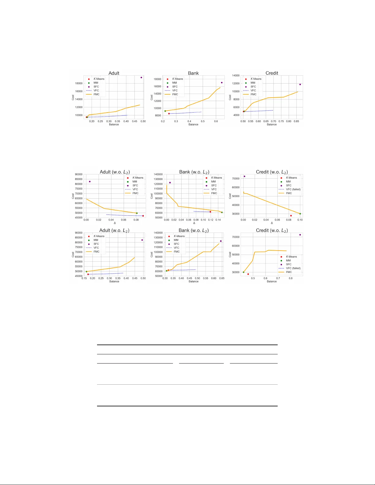
F air Model-Based Clustering Jinwon Park 1 , Kunw oong Kim 2 , Jihu Lee 2 , Y ongdai Kim 2 1 Graduate School of Data Science, Seoul National Univ ersity 2 Department of Statistics, Seoul National Univ ersity { jwpark127, kwkim.online, superstring1153, ydkim0903 } @gmail.com Abstract The goal of fair clustering is to ﬁnd clusters such that the proportion of sensitiv e attributes (e.g., gender, race, etc.) in each cluster is similar to that of the entire dataset. V arious fair clustering algorithms hav e been proposed that modify standard K-means clustering to satisfy a giv en fairness constraint. A critical limitation of several e xisting fair clustering algorithms is that the number of parameters to be learned is proportional to the sample size because the cluster assignment of each datum should be optimized simultaneously with the cluster center , and thus scaling up the algorithms is difﬁcult. In this paper , we propose a new fair clustering algorithm based on a ﬁnite mixture model, called Fair Model-based Clustering (FMC). A main advantage of FMC is that the number of learn- able parameters is independent of the sample size and thus can be scaled up easily . In particular , mini-batch learning is possible to obtain clusters that are approximately f air . More- ov er , FMC can be applied to non-metric data (e.g., categorical data) as long as the likelihood is well-deﬁned. Theoretical and empirical justiﬁcations for the superiority of the proposed algorithm are provided. Introduction Artiﬁcial intelligence (AI) systems have been increasingly deployed as decision support tools in socially sensiti ve do- mains such as credit scoring, criminal risk assessment, and college admissions. AI models trained on real-world data may inherently encode biases present in the training data. As a result, these models can exhibit discriminatory behavior or amplify historical biases (Feldman et al. 2015; Barocas and Selbst 2016; Chouldechov a 2017; Kleinberg et al. 2018; Mehrabi et al. 2021; Zhou et al. 2021). Numerous studies hav e shown that, in the presence of such unfairness, these systems tend to fav or majority groups, such as white men, while disadvantaging minority groups, such as black women. This can lead to unfair treatment of socially sensitiv e groups (Dua, Graff et al. 2017; Angwin et al. 2022). These ﬁndings underscore the need for fairness-a ware learning algorithms to mitigate bias in automated decision-making systems. Giv en these circumstances, it is crucial to prioritize fair - ness in automated decision-making systems to ensure that their de velopment is aligned with the principles of social responsibility . Consequently , a variety of algorithmic ap- proaches hav e been introduced to reduce bias by promoting equitable treatment of individuals across demographic groups. For instance, one common approach enforces f airness by re- quiring that the rates of fa vorable outcomes be approximately the same across groups deﬁned by sensitive attrib utes such as race or gender (Calders, Kamiran, and Pechenizkiy 2009; Gitiaux and Rangwala 2021; Zafar et al. 2017; Zeng et al. 2021; Agarwal et al. 2018; Donini et al. 2018; Zemel et al. 2013; Xu et al. 2018; Quadrianto, Sharmanska, and Thomas 2019). In parallel with advances in supervised learning, the study of algorithmic fairness in unsupervised learning, especially clustering, has garnered increasing attention. Clustering meth- ods hav e long been used for various machine learning appli- cations, including time series analysis (Lee, Choi, and Son 2024; Paparrizos and Grav ano 2016), audio and language modeling (Bro wn et al. 1992; Diez et al. 2019; Butnaru and Ionescu 2017; Zhang, W ang, and Shang 2023), recommenda- tion systems (Muhammad 2021; W idiyaningtyas, Hidayah, and Adji 2021), and image clustering (Le 2013; Guo et al. 2020; Mittal et al. 2022). Fair clustering (Chierichetti et al. 2017) aims to ensure that the proportion of each protected group within ev ery cluster is similar to that of the ov erall population. T o this end, a variety of algorithms ha ve been proposed to minimize a gi ven clustering objecti ve (e.g., K -means clustering cost) while satisfying predeﬁned fairness constraints (Bera et al. 2019; Backurs et al. 2019; Li, Zhao, and Liu 2020; Esmaeili et al. 2021; Ziko et al. 2021; Zeng et al. 2023). Most fair clustering algorithms are based on the K -means (center) algorithm which searches for good cluster centers and a good assignment map (mapping each instance to one of the gi ven cluster centers) under f airness constraints. A critical limitation of such existing f air clustering algorithms is that the fairness of a giv en assignment map depends on the entire training data and thus learning the optimal fair assignment map is computationally demanding. In fact, the assignment of each data point must be learned along with the cluster centers under a fairness constraint, so the number of learnable parameters is proportional to the sample size. Moreov er , a mini-batch learning algorithm, a typical tool to scale-up a giv en learning algorithm, would not be possible since the fairness of a gi ven assignment map cannot be e valuated on a mini-batch. Another limitation of existing fair clustering algorithms is that they are based on the K -means algorithm, which requires data to lie in a metric space, thus making it dif ﬁcult to process non-metric data such as categorical data. The aim of this study is to dev elop a new fair clustering algorithm that resolves the aforementioned limitations. The proposed algorithm is based on model-based clustering, and we estimate the parameters under a fairness constraint. Note that the existing methods are geometric and distance metric-based, yielding deterministic assignments, whereas model-based fair clustering assumes a probabilistic model for the data and uses likelihood-based estimation, pro viding probabilistic assignments. An important advantage of the proposed fair clustering algorithm is that the number of learnable parameters is inde- pendent of the size of training data and thus can be applied to large-scale datasets easily . Moreov er , the de velopment of a mini-batch algorithm to pro vide approximately fair clusters is possible with theoretical guarantees. In addition, non-metric data can be processed without much difﬁculty as long as the likelihood can be well-speciﬁed. The main contributions of this paper are summarized as follows. • W e propose a novel fair clustering algorithm based on a probabilistic model that f acilitates scalable mini-batch learning and dynamically recalculates fair assignments for large test datasets. • Unlike most existing f air clustering methods, our pro- posed algorithms are built upon a probabilistic mixture model and naturally extend to cate gorical data. • W e establish a theoretical guarantee that the proposed model generalizes well to unseen data, and v alidate it through comprehensiv e empirical ev aluations. Review of Existing F air Clustering Algorithms There are three cate gories of existing methods for fair clus- tering. (1) Pre-processing methods (Chierichetti et al. 2017; Backurs et al. 2019) use the concept of fairlets-small subsets of the data satisfying fairness-and then perform clustering on the space of fairlets. (2) In-processing methods (Kleindessner et al. 2019; Li, Zhao, and Liu 2020; Ziko et al. 2021; Zeng et al. 2023; Kim et al. 2025) optimize both the assignments and cluster centers to ﬁnd a good clustering among those satisfying a giv en fairness le vel. (3) Post-processing meth- ods (Bera et al. 2019; Harb and Lam 2020) only build fair assignments for ﬁxed cluster centers. Here, we brieﬂy revie w in-processing methods to explain the limitations of existing fair clustering algorithms. Let D = { x 1 , . . . , x N } be the given training data to be clustered, and let s 1 , . . . , s N be sensitiv e attributes corre- sponding to x 1 , . . . , x N , where s i ∈ [ M ] for all i ∈ [ N ] . Here, M is the number of sensitiv e groups. Let D ( s ) = { x i ∈ D : s i = s } for s ∈ [ M ] . W e ﬁrst focus on the case M = 2 for the following discussion, and propose a way of extend- ing the algorithm in the Modiﬁcation of FMC to multinary sensitive attributes section. A typical clustering algorithm (without a fairness con- straint) recei ves D and the number of clusters K as inputs and yields the cluster centers µ k , k ∈ [ K ] , and the assign- ment map A : D → [ K ] such that A ( x i ) is the cluster to which x i belongs. The algorithm searches { µ k , k ∈ [ K ] } and A that minimizes the clustering cost L ( D ; K ) := P N i =1 ρ ( x i , µ A ( x i ) ) for a gi ven metric ρ. A fair clustering algorithm receives D ( s ) , s ∈ [2] and K as inputs and searches µ k , k ∈ [ K ] and A that minimize L ( D ; K ) subject to the constraint that A is fair , i.e., |{ i : A ( x i ) = k , s i = 1 }| / N 1 ≈ |{ i : A ( x i ) = k , s i = 2 }| / N 2 for all k ∈ [ K ] , where N s = |D ( s ) | . In certain cases, fair assignment maps do not e xist. T o ensure existence, we con- sider a soft assignment map A sof t : D → S K , where S K is the ( K − 1) -dimensional simplex (Kim et al. 2025). Here, A sof t ( x i ) k is interpreted as the probability of x i belonging to cluster k . A typical procedure for in-processing fair clustering algo- rithms is summarized as follows. A f air clustering algorithm ﬁrst ﬁnds the cluster centers using a fairness-agnostic clus- tering algorithm. It then updates the (soft) assignment map while the cluster centers are ﬁxed. In turn, it updates the clus- ter centers while the assignment map is ﬁxed, and it repeats these two updates iterati vely until con vergence. A problem in such fair clustering algorithms is that updat- ing the assignment map is computationally demanding when the sample size is large, as the full optimization has cubic complexity: the number of learnable parameters is N , since A ( x i ) , i ∈ [ N ] must be updated simultaneously . Moreover , a mini-batch algorithm—a typical way to scale-up a learn- ing procedure—is not possible, since the fairness of a gi ven assignment map depends on the entire dataset. Another problem arises when assigning test data to clusters. Assigning ne wly arri ved data f airly after learning fair clusters is challenging, because the learned assignment map is deﬁned only on the training data. A practical solution would be to obtain the optimal assignment map for test data while the cluster centers are ﬁxed. This nai ve solution, ho wev er , is not applicable when test data arriv e sequentially . The aim of this paper is to propose a new fair clustering algorithm whose number of parameters is independent of the size of the training data and is thus easy to scale-up. Moreov er , it is possible to develop a mini-batch algorithm to provide an approximately fair clustering with theoretical guarantees. In addition, the algorithm yields a parameterized assignment map, and thus assigning newly arriv ed unseen data is easy . Finite Mixture Models One renowned model-based clustering method is the ﬁnite mixture model, which assumes that x 1 , . . . , x N ∈ R d are independent realizations of a d -dimensional random variable X with density giv en by X ∼ f ( · ; Θ) := K X k =1 π k f ( · ; θ k ) , (1) where K is the number of mixture components and f ( · ; θ k ) is the density of a parametric distribution with parameter θ k for k ∈ [ K ] . The Gaussian distribution is commonly used for f ( · ; θ ) but other parametric distrib utions can also be used (e.g., the categorical (multinoulli) distribution for cate gorical data). The mixture weight v ector π = ( π 1 , . . . , π K ) lies on the ( K − 1) -dimensional simple x. From a clustering perspec- ti ve, K is the number of clusters; f ( · ; θ k ) is the density of the k th component (cluster); and π k is the probability of belong- ing to the k th cluster . The parameter Θ = ( π , ( θ 1 , . . . , θ K )) can be estimated by maximum likelihood (MLE), which max- imizes the log-likelihood gi ven by ℓ (Θ | D ) = N X i =1 log K X k =1 π k f ( x i ; θ k ) ! . V arious algorithms have been proposed to compute the MLE in the ﬁnite mixture model. Among these, the Expectation- Maximization (EM) algorithm (T itterington, Smith, and Mako v 1985; Xu and Jordan 1996a; W u 1983a) and gradient- descent-based (GD) optimization algorithm (Gepperth and Pf ¨ ulb 2021; Hosseini and Sra 2020) are most widely used. Xu and Jordan (1996b) showed that EM and GD for the ﬁnite mixture model are linked via a projection matrix. An adv an- tage of EM is that the objective function is monotonically increasing without the need to set a learning rate. In contrast, GD is more ﬂexible and applicable to a broader range of differentiable objecti ves. Assignment Map f or the Finite Mixture Model An equiv alent formulation of the ﬁnite mixture model in Eq. (1) is giv en by: Z 1 , . . . , Z N i.i.d. ∼ Categorical( π ) X i | Z i ∼ f ( · ; θ Z i ) , i ∈ [ N ] . Here, from a clustering perspecti ve, Z i is interpreted as the cluster index to which x i belongs. Note that p ( Z i = k | X i = x i ; Θ) = π k f ( x i ; θ k ) P K l =1 π l f ( x i ; θ l ) . (2) In this paper , we use (2) as the (soft) assignment map cor- responding to the ﬁnite mixture model with parameter Θ and denote it by ψ k ( x i ; Θ) = p ( Z i = k | X i = x i ; Θ) for k ∈ [ K ] . In practice, the hard assignment map ψ hard ( x i ; Θ) for any gi ven x i can be determined from the soft assignment map via ψ hard ( x i ; Θ) = argmax k ∈ [ K ] { ψ k ( x i ; Θ) } . In the case of the Gaussian mixture model, this hard assignment map is close to the optimal assignment map of the K -center algorithm under regularity conditions. See Theorem 6 in the Appendix for a detailed discussion. Learning a F air Finite Mixture Model F airness Constraint f or the Finite Mixture Model Let C = { C 1 , . . . , C K } denote a giv en set of clusters of D where C k = { x i ∈ D : Z i = k } is the k th cluster of D . Let C 1 = { C 1 1 , . . . , C 1 K } and C 2 = { C 2 1 , . . . , C 2 K } denote the sets of clusters of D (1) and D (2) , respectiv ely , where C k = C 1 k ∪ C 2 k . The most commonly used fairness measure in clustering is Balance (Chierichetti et al. 2017), which is the minimum of the ratios of each sensitive attrib ute in ev ery cluster . The Balance of C = { C 1 , . . . , C K } is deﬁned as min k ∈ [ K ] min  | C 1 k | / | C 2 k | , | C 2 k | / | C 1 k |  . (3) Smaller Balance indicates less fair clusters, and vice versa. Bera et al. (2019) studied a clustering algorithm that ﬁnds optimal clusters under a Balance constraint by constructing fair assignments. A similar but numerically easier measure for fairness than Balance is a dif ference-based rather than ratio-based measure. That is, we deﬁne Gap as max k ∈ [ K ]     | C 1 k | N 1 − | C 2 k | N 2     . (4) A larger Gap means less fairness of clusters and vice v ersa. Kim et al. (2025) considered the additi ve version of Gap deﬁned by X k ∈ [ K ]     | C 1 k | N 1 − | C 2 k | N 2     , (5) and dev eloped a fair clustering algorithm. A natural extension of Gap for the assignment map ψ k ( · ; Θ) , k ∈ [ K ] , is ∆(Θ) := max k ∈ [ K ]      P x i ∈D (1) ψ k ( x i ; Θ) N 1 − P x j ∈D (2) ψ k ( x j ; Θ) N 2      . (6) In this paper , we propose to estimate Θ under the constraint ∆(Θ) ≤ ε for a prespeciﬁed fairness le vel ε ≥ 0 (the smaller ε, the fairer). That is, the objecti ve of our proposed fair clus- tering is: max Θ ℓ (Θ | D ) subject to ∆(Θ) ≤ ε. (7) Giv en a Lagrange multiplier λ ≥ 0 , we can alternatively maximize ℓ (Θ | D ; λ ) := ℓ (Θ | D ) − λ ∆(Θ) . W e abbreviate ∆(Θ) as ∆ where appropriate. For the algorithms presented belo w , we identify the max- imizing index k in Eq. (6) and then ev aluate ∆ using that k . W e use Gap instead of Balance for numerical sta- bility when applying gradient-descent optimization. Re- garding the relationship between Balance and Gap, we note that: (i) (Kim et al. 2025) theoretically sho wed that | Balance − min( n 0 /n 1 , n 1 /n 0 ) | ≤ Additi ve Gap in Eq. (5) (where min( n 0 /n 1 , n 1 /n 0 ) is the balance of perfectly fair clustering), and (ii) our numerical experiments sho w that smaller ∆ corresponds to a larger Balance (Fig. 11 in the Appendix). Learning Algorithms: FMC-GD and FMC-EM T o optimize the objectiv e in Eq. (7), we employ gradient- descent (GD) and expectation–maximization (EM) algo- rithms, with pseudocode in Algorithms 1 and 2. W e here- after refer to these as FMC-GD (Fair Model-based Clustering with Gradient Descent) and FMC-EM (Fair Model-based Clustering with Expectation–Maximization), respectiv ely . Algorithm 1 FMC-GD (Gradient-Descent) In practice, we set ( T , γ ) = (10000 , 10 − 3 ) Input : Dataset D = { x 1 , . . . , x N } , Number of clusters K , Lagrange multiplier λ , Maximum number of iterations T and Learning rate γ . Initialize : Θ [0] = ( η [0] , θ [0] ) while Θ has not con verged and t < T do θ [ t +1] ← θ [ t ] − γ ∂ ∂ θ  − ℓ (Θ [ t ] | X ) + λ ∆(Θ [ t ] )  η [ t +1] ← η [ t ] − γ ∂ ∂ η  − ℓ (Θ [ t ] | X ) + λ ∆(Θ [ t ] )  π [ t +1] ← softmax ( η [ t +1] ) t ← t + 1 end while (1) FMC-GD FMC-GD maximizes ℓ (Θ | D ; λ ) using gradient-descent-based optimization. T o improve numeri- cal stability of the gradients, we reparameterize the mixture weights as π = softmax( η ) . The gradient formulas used in Algorithm 1 are pro vided in the Appendix, in the section Derivation of the Gradients in Algorithm 1 . (2) FMC-EM F or FMC-EM, we consider the complete- data Y = ( D , Z ) , where Z = ( Z 1 , . . . , Z N ) ⊤ , along with the complete-data log-likelihood ℓ comp (Θ | Y ) : ℓ comp (Θ | Y ) = N X i =1 K X k =1 I ( Z i = k ) { log π k + log f ( x i ; θ k ) } . (8) As in the standard EM algorithm, FMC-EM iterates the E- step and M-step. Let Θ [ t ] be the updated parameter at the t th iteration. Giv en D and Θ [ t ] , the Q function (computed in the E-step and maximized in the M-step) is Q (Θ | Θ [ t ] ) = E Z |D ;Θ [ t ] ℓ comp (Θ | Y ) . (9) See Eq. (42) in the Appendix for a detailed deri vation of Q (Θ | Θ [ t ] ) . For FMC-EM, the Q function is modiﬁed to Q f air (Θ | Θ [ t ] ; λ ) = E Z |D , Θ [ t ] ( ℓ comp (Θ | Y ) − λ ∆(Θ)) . (10) W e compute Q f air in the E-step and update Θ to maximize Q f air in the M-step. Since maximizing Q f air admits no closed-form solution, we instead apply gradient-based op- timization to ensure an increase at each iteration. This pro- cedure is a special case of the Generalized EM (GEM) al- gorithm (Dempster , Laird, and Rubin 1977), which requires only that each update of Θ increase the Q function. T o sum up, gi ven Θ [ t ] at the t th iteration, we update the parameters Θ [ t +1] via gradient-descent-based optimization, choosing the learning rate to satisfy Q f air (Θ [ t +1] | Θ [ t ] ; λ ) ≥ Q f air (Θ [ t ] | Θ [ t ] ; λ ) . (11) See Fig. 10 in the Appendix for the empirical con ver gence of FMC-EM. Mini-Batch Learning with Sub-Sampled ∆ When the size of the dataset is large, reducing computational cost becomes a critical concern, and the use of mini-batches Algorithm 2 FMC-EM (Expectation-Maximization) In practice, we set ( T , R, γ ) = (200 , 10 , 10 − 2 ) Input: Dataset D = { x 1 , . . . , x N } , Number of clusters K , Lagrange multiplier λ , Maximum numbers of iterations T , R and Learning rate γ . Initialize: Θ [0] = ( η [0] , θ [0] ) while Q f air has not con verged and t < T do Compute Q f air (Θ | Θ [ t ] ; λ ) in Eq. (10) while r < R do θ [ t ] ( r +1) ← θ [ t ] ( r ) − γ ∂ ∂ θ  − Q f air (Θ; Θ [ t ] , λ )  η [ t ] ( r +1) ← η [ t ] ( r ) − γ ∂ ∂ η  − Q f air (Θ; Θ [ t ] , λ )  π [ t ] ( r +1) ← softmax ( η [ t ] ( r +1) ) r ← r + 1 end while θ [ t +1] ← θ [ t ] ( R ) π [ t +1] ← π [ t ] ( R ) t ← t + 1 end while can be a compelling approach. The objective function of FMC consists of two terms: the log-likelihood and the fairness penalty term ∆ . Ho wev er , note that a mini-batch algorithm can be applied to the log-likelihood term b ut cannot be easily applied to ∆ . Hence, we need a technique to reduce the computational cost of computing the gradient of ∆ . For this purpose, we use the fact that ∆ can be closely approximated by its v alue on sub-sampled data. Let D n be a dataset of size n obtained by randomly sampling n data points from D , and let ∆(Θ; D n ) be the ∆ computed on D n . Under regularity conditions, it can be sho wn that fair clus- ters under the sub-sampled ∆ constraint are approximately fair in terms of the (population) ∆ constraint. For simplicity , we focus on the Gaussian mixture model: let f ( x ; θ ) be a Gaussian distribution with mean vector µ and cov ariance matrix Σ , and thus Θ = ( π , (( µ 1 , Σ 1 ) , . . . , ( µ K , Σ K ))) . For giv en positi ve constants ξ , ζ and ν, let Φ ξ,ζ ,ν = { Θ : ξ < min k { π k } ≤ max k { π k } < 1 − ξ , max k ∥ µ k ∥ ≤ ν, ζ < min k λ min (Σ k ) ≤ max k λ max (Σ k ) < 1 /ζ } , where λ min and λ max are the smallest and largest eigen values, respec- tiv ely . The following proposition gi ves a bound on the error between ∆(Θ; D n ) and ∆(Θ) . T o av oid technical difﬁculties, we assume that D n is obtained by sampling with replacement from D . The proof is gi ven in the Appendix. Proposition 1. Let n s = |{ x i ∈ D n : s i = s }| for s ∈ { 1 , 2 } . Then, with pr obability at least 1 − δ, we have sup Θ ∈ Φ ξ,ζ ,ν | ∆(Θ) − ∆(Θ; D n ) | ≤ 4 C r d n ′ + 8 r 2 log(8 /δ ) n ′ (12) for some constant C = C ( ξ , ζ , ν, x max ) , wher e x max = max x ∈D ∥ x ∥ 2 and n ′ = min { n 1 , n 2 } . Motiv ated by Proposition 1, we propose to estimate Θ by maximizing ℓ (Θ | D ) − λ ∆(Θ; D n ) , where we apply mini-batch learning to the term ℓ (Θ | D ) while D n is ﬁxed. In FMC-GD, we take gradient steps for ℓ (Θ | D ) on a giv en mini-batch, whereas in FMC-EM, we compute ℓ comp (Θ | Y ) in the E-step only on a giv en mini- batch. See Algorithm 3 in the Appendix for details of the mini- batch learning algorithm with the sub-sampled ∆ constraint. Moreov er , Karimi, La vielle, and Moulines (2019) studied con vergence properties of the mini-batch EM algorithm, and we sho w a similar result for the mini-batch GEM in Theo- rem 7 in the Appendix. W e emphasize that neither mini-batch learning nor a sub- sampled fairness constraint is possible in existing fair clus- tering algorithms, since the assignment map for the entire dataset must be learned simultaneously . The key inno vation of the proposed fair ﬁnite mixture model is to use the para- metric model in Eq. (2) as the (soft) assignment map. Note that learning the parameters is computationally easier than directly learning the assignment map for the entire dataset. Sub-Sample Learning Another advantage of FMC is that the functional form of the assignment map is av ailable after training, which allows us to fairly assign newly arrived data (which are not av ail- able during the learning of Θ ) to clusters. That is, we assign an unseen datum x to cluster k with probability ψ k ( x ; ˆ Θ) , where ˆ Θ is the estimated parameter v ector . Howe ver , this fair post-assignment is not possible for existing fair clustering algorithms, since the assignment map is deﬁned only for the training data. The fair post-assignment also enables learning the fair mixture model on randomly selected sub-samples when the entire dataset is too large. Speciﬁcally , we estimate Θ on ran- domly selected sub-samples D n of size n from D , and then assign the data in D \ D n using the estimated assignment map { ψ k ( x ; ˆ Θ) } k ∈ [ K ] . Proposition 1 guarantees that the clusters obtained in this way are approximately fair . In the Numerical experiments section, we empirically sho w that the reduction in performance, as measured by clustering cost and ∆ , due to sub-sampling is minimal, unless n is too small. Numerical Experiments In our numerical experiments, we ev aluate FMC by analyz- ing sev eral real-world datasets: (i) on three moderate-scale real datasets, we show that FMC is competitiv e with base- line methods; and (ii) on a lar ge-scale dataset consisting of millions of instances, FMC outperforms the baselines while requiring signiﬁcantly less computational time. In addition, we in vestigate mini-batch learning and sub-sample learning of FMC, and show that the two algorithms perform similarly when the sub-sample size is not too small (e.g., 5%). W e additionally conduct parameter impact studies on (i) the number of clusters K and (ii) the choice of covariance structure when f is a Gaussian mixture. Experimental Settings Datasets W e use four real-world datasets: Adult, Bank, Credit, and Census datasets, which are all av ailable in the UCI Machine Learning Repository 1 . Brief descriptions of the datasets are giv en below , with details in the Appendix. • Adult dataset: UCI Adult (1994 US Census), 32,561 sam- ples; 5 continuous and 8 categorical features; sensitive attribute: gender (male 66.9%, female 33.1%). • Bank dataset: UCI Bank Marketing, 41,008 samples; 6 continuous and 10 categorical features; sensitiv e attribute: marital status (married 60.6%, unmarried 39.4%). • Credit dataset: UCI Default of Credit Card Clients, 30,000 samples; 4 continuous and 8 categorical features; sensitiv e attribute: education, aggre gated into two groups (46.8% vs. 53.2%) or three groups (46.8%, 35.3%, 17.9%). • Census dataset: UCI Census (1990 US Census), 2,458,285 samples; 25 features; sensiti ve attribute: gender (male 51.53%, female 48.47%). W e analyze only the continuous variables in the main anal- ysis, since we focus on the Gaussian mixture model. Subse- quently , we include categorical data to v alidate the applica- bility of FMC to categorical variables. W e standardize the continuous v ariables to hav e zero mean and unit variance. Then, we apply L 2 normalization to the standardized data (i.e., so that each datum has unit L 2 norm), because VFC (Ziko et al. 2021), one of the baseline methods, often fails to con verge without L 2 normalization. Numerical results with- out L 2 normalization are giv en in the Appendix. Algorithms For continuous data, we use the Gaussian mix- ture model (GMM) for f with an isotropic cov ariance matrix σ 2 I d . That is, the complete-data log-likelihood of the GMM is deriv ed as ℓ comp (Θ | Y ) = N X i =1 K X k =1 I ( Z i = k )  log π k − d log(2 π σ 2 ) 2 − ∥ x i − µ k ∥ 2 2 2 σ 2  , (13) where Θ = ( π , ( µ , σ )) . For categorical data, we use the categorical (multinoulli) mixture model; details are gi ven in Eqs. (84) and (85) in the Appendix. For fair clustering baseline methods, we consider three existing methods: SFC, VFC, and FCA. SFC (Backurs et al. 2019) is a scalable fair clustering algorithm based on f airlet decomposition, yielding near-perfectly f air clustering. VFC (Ziko et al. 2021) performs fair clustering by adding a v ari- ational fairness constraint based on the Kullback–Leibler (KL) di vergence. FCA (Kim et al. 2025) is a recently de vel- oped state-of-the-art method that performs fair clustering by matching distributions across dif ferent groups. In addition, for f airness-unaware clustering methods, we consider K -means and Gaussian mixture models learned with EM or GD (denoted MM-EM and MM-GD). Evaluation For fairness metrics, we consider ∆ and Bal- ance, and for clustering utility metrics, we consider Cost (the sum of distances from each data point to its assigned cluster center). For FMC, we use the hard assignment map when computing the fairness metrics to ensure comparability , since SFC and VFC only yield hard assignments. 1 https://archiv e.ics.uci.edu/datasets Figure 1: Pareto front lines between ∆ and Cost on Adult, Bank, and Credit datasets. See Fig. 5 for the lines between Balance and Cost. See Fig. 6 for the similar results without L 2 normalization. Initial parameters W e set the initial value of mixture weights to π = (1 /K, . . . , 1 /K ) ⊤ . The initial means µ are set to the cluster centers obtained by the K -means algorithm with random initialization. For the v ariance, we set σ = 1 . 0 . See the Appendix for additional implementation details. Perf ormance Comparison Comparing FMC-EM and FMC-GD Fig. 2 presents Pareto front plots of ∆ versus Cost (with standard devia- tion bands from ﬁv e random initializations) for FMC-EM and FMC-GD on the Adult dataset. It sho ws that FMC-EM achie ves a better cost-fairness trade-of f with smaller v ariance. Accordingly , we use FMC-EM for subsequent e xperiments and, where appropriate, refer to it simply as FMC . Figure 2: Pareto front lines between ∆ and Cost (with stan- dard deviation bands obtained by ﬁ ve random initializations) of FMC-EM (left ) and FMC-GD (right) on Adult dataset. See Fig. 4 in Appendix for similar results with respect to Balance and on other datasets. FMC vs. Baseline algorithms Fig. 1 shows the Pareto front plots of ∆ versus Cost. Note that SFC operates only at (near-perfect) f airness and therefore appears as a single point. These results lead to two observ ations. (i) FMC is better than SFC in terms of Cost at a near- perfect fairness le vel. This is not surprising, since FMC learns the cluster centers and the fair assignment map simultane- ously , whereas SFC learns them sequentially . An additional advantage of FMC over SFC is the ability to control the fairness le vel, whereas SFC cannot. (ii) VFC is slightly superior to FMC with respect to the cost–fairness trade-of f. This is expected because VFC min- imizes Cost explicitly whereas FMC maximizes the log- likelihood, which is only indirectly related to Cost. On the other hand, VFC fails to control the fairness le vel across the entire range. For e xample, VFC does not provide a fair clus- tering with ∆ < 0 . 06 on the Bank dataset. Another adv antage of FMC over VFC is rob ustness to data pre-processing meth- ods. As previously discussed, we apply L 2 normalization, since VFC fails to con ver ge without it on the Credit and Cen- sus datasets (see Figs. 6 and 7 in the Appendix). W e note that L 2 normalization is not a standard pre-processing step, since it maps points onto the unit sphere. In this sense, FMC is more broadly applicable. See T able 3 in the Appendix for additional comparisons between FMC and FCA. Analysis on Large-Scale Dataset This section provides experimental results on the Census dataset, a large-scale dataset consisting of more than 2 million samples. FMC vs. Baseline algorithms For FMC, we apply mini- batch learning with a sub-sampled ∆ , where the mini-batch and sub-sample sizes are set to 10% of the full dataset. Fig. 3 displays the results, showing that FMC is competiti ve with VFC and better than SFC. In addition, consistent with the results on moderate-scale data, FMC retains the adv antage of controlling the fairness lev el across the entire range. More- ov er , FMC with mini-batch learning reduces computation time signiﬁcantly (e.g., about 20x faster than VFC), as sho wn in T able 1. Figure 3: Pareto front lines between { ∆ , Balance } and Cost on Census dataset. See Fig. 7 in Appendix for the similar results without L 2 normalization. Algorithm T ime (std) VFC 5053.0 (915.5) SFC 2218.2 (535.1) FMC (mini-batch, n = 0 . 1 N ) 253.0 (12.1) T able 1: Comparison of the a verage computation time (sec- onds) with standard deviations (std) ov er ﬁv e random initials on Census dataset ( N = 2,458,285). Mini-batch learning vs. Sub-sample learning W e fur- ther inv estigate whether sub-sample learning empirically performs similarly to mini-batch learning by v arying the sub-sample sizes in { 1% , 3% , 5% , 10% } . For example, when training with 5% sub-samples, we e valuate the learned model on the full dataset (i.e., perform inference on t he remaining 95% of the data and then aggregate the inferred assignments with those of the training data). T able 2 compares the perfor- mance of (i) sub-sample learning (sizes { 1% , 3% , 5% , 10% } ) and (ii) mini-batch learning with batch size 10% . Sub-sample learning with size ≥ 5% yields performance similar to mini- batch learning but with lo wer computational cost. These re- sults suggest that sub-sample learning is useful when the dataset is very lar ge. Method  n N  Cost ( × 10 5 ) ∆ Balance T ime SS (1%) 11.167 0.005 0.851 53.7% SS (3%) 10.988 0.004 0.894 65.8% SS (5%) 10.973 0.003 0.883 71.4% SS (10%) 10.916 0.003 0.881 77.2% MB (10%) 10.857 0.002 0.896 100.0% T able 2: Performances of mini-batch learning (MB) and sub- sample learning (SS) on Census dataset. The computation times of SS are measured by the relative ratio compared to the mini-batch learning with 10% , and the Lagrangian λ for each case is tuned to achieve the lo west Gap value i.e., ∆ ≈ 0 . See T able 4 in Appendix for the similar results without L 2 normalization. Categorical Data Analysis An additional advantage of FMC is the ability to incorpo- rate categorical data into clustering by using the cate gorical (multinoulli) mixture model, whose formulation is gi ven in Eqs. (84) and (85) in the Appendix. T ables 5 and 6 in the Appendix show that FMC performs well with categorical data. Note that the baseline methods do not nati vely handle categorical v ariables; nontrivial modiﬁcations are required. Modiﬁcation of FMC f or Multinary Sensitive Attributes T o apply FMC to multinary sensitiv e attributes, i.e., M > 2 , we propose the following modiﬁcation of ∆ : max k ∈ [ K ] 2 M ( M − 1) X s 1 ,s 2 ∈ [ M ] s 1  = s 2 ∆ s 1 ,s 2 , (14) where ∆ s 1 ,s 2 :=      P x i ∈D ( s 1 ) ψ k ( x i ; Θ) N s 1 − P x i ∈D ( s 2 ) ψ k ( x i ; Θ) N s 2      . (15) T able 7 in the Appendix compares VFC and FMC on Bank and Credit datasets where the sensiti ve attribute has three categories. See the e xperimental details in the Appendix. The results conﬁrm that the modiﬁed FMC performs well. Parameter Impact Studies The number of clusters K W e analyze ho w the number of clusters K affects the performance of FMC, and we ﬁnd that FMC performs well regardless of the choice of K. That is, the ne gati ve log-likelihood decreases as K in- creases, while the fairness le vel ∆ remains sufﬁciently lo w . See Fig. 8 in the Appendix for the results. Choice of covariance structure in GMM W e consider a diagonal cov ariance matrix instead of the isotropic one in the GMM to assess whether a more ﬂexible cov ariance structure improv es clustering. Fig. 9 in the Appendix suggests that the diagonal cov ariance matrix is generally beneﬁcial, which is an additional advantage of FMC o ver SFC and VFC. Discussion In this work, we hav e proposed FMC, a ﬁnite mixture model based fair clustering algorithm, which can be easily scaled- up through mini-batch and sub-sample learning. Moreov er , FMC can handle both continuous and categorical data. The main idea of FMC is to parameterize the assignment map. W e leave the application of this idea to existing fair clustering algorithms (e.g., VFC) for future work. Choosing the number of clusters K is also important. There is extensi ve research on estimating K in ﬁnite mixture models (Schwarz 1978; Biernacki, Celeux, and Go vaert 2002; Richardson and Green 1997; Miller and Harrison 2018). W e will in vestigate ho w to adapt these estimators to fair cluster - ing in future work. Acknowledgements This work was partly supported by the National Research Foundation of K orea (NRF) grant funded by the K orea gov- ernment (MSIT) (No. 2022R1A5A7083908); Institute of In- formation& communications T echnology Planning & Evalu- ation (IITP) grant funded by the K orea government (MSIT) (No.RS-2022-II220184, Dev elopment and Study of AI T ech- nologies to Inexpensiv ely Conform to Evolving Policy on Ethics); Institute of Information & communications T ech- nology Planning & Evaluation (IITP) grant funded by the K orea government (MSIT) [NO.RS-2021-II211343; Artiﬁ- cial Intelligence Graduate School Program (Seoul National Univ ersity)], and the National Research Foundation of K o- rea (NRF) grant funded by the Korea gov ernment (MSIT) (RS-2025-00556079). References Agarwal, A.; Be ygelzimer , A.; Dud ´ ık, M.; Langford, J.; and W allach, H. 2018. A reductions approach to fair classiﬁca- tion. In International confer ence on machine learning , 60–69. PMLR. Angwin, J.; Larson, J.; Mattu, S.; and Kirchner , L. 2022. Machine bias. In Ethics of data and analytics , 254–264. Auerbach Publications. Backurs, A.; Indyk, P .; Onak, K.; Schieber , B.; V akilian, A.; and W agner, T . 2019. Scalable fair clustering. In Interna- tional confer ence on machine learning , 405–413. PMLR. Barocas, S.; and Selbst, A. D. 2016. Big data’ s disparate impact. Calif. L. Rev . , 104: 671. Bera, S.; Chakrabarty , D.; Flores, N.; and Negahbani, M. 2019. Fair algorithms for clustering. Advances in Neural Information Pr ocessing Systems , 32. Biernacki, C.; Celeux, G.; and Gov aert, G. 2002. Assessing a mixture model for clustering with the integrated completed likelihood. IEEE transactions on pattern analysis and ma- chine intelligence , 22(7): 719–725. Bro wn, P . F .; Della Pietra, V . J.; deSouza, P . V .; Lai, J. C.; and Mercer , R. L. 1992. Class-Based n -gram Models of Natural Language. Computational Linguistics , 18(4): 467–480. Butnaru, A. M.; and Ionescu, R. T . 2017. From image to text classiﬁcation: A nov el approach based on clustering word embeddings. Pr ocedia computer science , 112: 1783–1792. Calders, T .; Kamiran, F .; and Pechenizkiy , M. 2009. Building classiﬁers with independency constraints. In 2009 IEEE international confer ence on data mining workshops , 13–18. IEEE. Chierichetti, F .; Kumar , R.; Lattanzi, S.; and V assilvitskii, S. 2017. Fair clustering through fairlets. Advances in neural information pr ocessing systems , 30. Chouldechov a, A. 2017. Fair prediction with disparate im- pact: A study of bias in recidi vism prediction instruments. Big data , 5(2): 153–163. Dempster , A. P .; Laird, N. M.; and Rubin, D. B. 1977. Maxi- mum likelihood from incomplete data via the EM algorithm. Journal of the r oyal statistical society: series B (methodolog- ical) , 39(1): 1–22. Diez, M.; Burget, L.; W ang, S.; Rohdin, J.; and ˇ Cernock ´ y, J. 2019. Bayesian HMM Based x-V ector Clustering for Speaker Diarization. In Interspeech 2019 , 346–350. Donini, M.; Oneto, L.; Ben-David, S.; Shawe-T aylor , J. S.; and Pontil, M. 2018. Empirical risk minimization under fair- ness constraints. Advances in neural information pr ocessing systems , 31. Dua, D.; Graff, C.; et al. 2017. UCI machine learning reposi- tory , 2017. URL http://arc hive.ics.uci.edu/ml , 7(1): 62. Ac- cessed: 2025-01-10. Esmaeili, S.; Brubach, B.; Srini vasan, A.; and Dick erson, J. 2021. Fair clustering under a bounded cost. Advances in Neural Information Pr ocessing Systems , 34: 14345–14357. Feldman, M.; Friedler , S. A.; Moeller , J.; Scheidegger , C.; and V enkatasubramanian, S. 2015. Certifying and removing disparate impact. In pr oceedings of the 21th ACM SIGKDD international confer ence on knowledge discovery and data mining , 259–268. Gepperth, A.; and Pf ¨ ulb, B. 2021. Gradient-Based T raining of Gaussian Mixture Models for High-Dimensional Streaming Data. Neural Pr ocess. Lett. , 53(6): 4331–4348. Gitiaux, X.; and Rangwala, H. 2021. Learning Smooth and Fair Representations. In Banerjee, A.; and Fukumizu, K., eds., Pr oceedings of The 24th International Conference on Artiﬁcial Intelligence and Statistics , v olume 130 of Pr oceed- ings of Machine Learning Resear ch , 253–261. PMLR. Guo, J.; Zhu, X.; Zhao, C.; Cao, D.; Lei, Z.; and Li, S. Z. 2020. Learning meta face recognition in unseen domains. In Pr oceedings of the IEEE/CVF Conference on Computer V ision and P attern Recognition , 6163–6172. Harb, E.; and Lam, H. S. 2020. KFC: A Scalable Approxima- tion Algorithm for k-center Fair Clustering. In Larochelle, H.; Ranzato, M.; Hadsell, R.; Balcan, M.; and Lin, H., eds., Ad- vances in Neur al Information Pr ocessing Systems , v olume 33, 14509–14519. Curran Associates, Inc. Hosseini, R.; and Sra, S. 2020. An alternative to EM for Gaussian mixture models: batch and stochastic Riemannian optimization. Math. Pr ogram. , 181(1): 187–223. Karimi, B.; Lavielle, M.; and Moulines, ´ E. 2019. On the Con vergence Properties of the Mini-Batch EM and MCEM Algorithms. W orking paper or preprint. Kim, K.; Lee, J.; Park, S.; and Kim, Y . 2025. Fair Clustering via Alignment. Kleinberg, J.; Ludwig, J.; Mullainathan, S.; and Rambachan, A. 2018. Algorithmic fairness. In Aea papers and pr oceed- ings , volume 108, 22–27. American Economic Association 2014 Broadway , Suite 305, Nashville, TN 37203. Kleindessner , M.; Samadi, S.; A wasthi, P .; and Mor genstern, J. 2019. Guarantees for spectral clustering with f airness constraints. In International confer ence on machine learning , 3458–3467. PMLR. Le, Q. V . 2013. Building high-level features using large scale unsupervised learning. In 2013 IEEE international confer ence on acoustics, speec h and signal pr ocessing , 8595– 8598. IEEE. Lee, S.; Choi, C.; and Son, Y . 2024. Deep time-series clus- tering via latent representation alignment. Knowledge-Based Systems , 303: 112434. Li, P .; Zhao, H.; and Liu, H. 2020. Deep fair clustering for visual learning. In Pr oceedings of the IEEE/CVF Confer ence on Computer V ision and P attern Recognition , 9070–9079. Mehrabi, N.; Morstatter, F .; Saxena, N.; Lerman, K.; and Galstyan, A. 2021. A survey on bias and fairness in machine learning. ACM computing surve ys (CSUR) , 54(6): 1–35. Miller , J. W .; and Harrison, M. T . 2018. Mixture models with a prior on the number of components. Journal of the American Statistical Association , 113(521): 340–356. Mittal, H.; Pande y , A. C.; Saraswat, M.; Kumar , S.; Pal, R.; and Modwel, G. 2022. A comprehensiv e survey of image segmentation: clustering methods, performance parameters, and benchmark datasets. Multimedia T ools and Applications , 81(24): 35001–35026. Mohri, M.; Rostamizadeh, A.; and T alwalkar , A. 2018. F oun- dations of machine learning . MIT press. Muhammad, M. 2021. Recommendation System Using User - Based Collaborativ e Filtering and Spectral Clustering. EAI. Nesterov , Y . 2013. Gradient methods for minimizing compos- ite functions. Mathematical pr ogramming , 140(1): 125–161. Paparrizos, J.; and Gra vano, L. 2016. k-Shape: Efﬁcient and Accurate Clustering of T ime Series. SIGMOD Rec. , 45(1): 69–76. Quadrianto, N.; Sharmanska, V .; and Thomas, O. 2019. Dis- cov ering Fair Representations in the Data Domain. In Pro- ceedings of the IEEE/CVF Confer ence on Computer V ision and P attern Recognition (CVPR) . Richardson, S.; and Green, P . J. 1997. On Bayesian analysis of mixtures with an unkno wn number of components (with discussion). Journal of the Royal Statistical Society Series B: Statistical Methodology , 59(4): 731–792. Robbins, H.; and Siegmund, D. 1971. A conv ergence the- orem for non neg ativ e almost supermartingales and some applications. In Optimizing methods in statistics , 233–257. Elsevier . Schwarz, G. 1978. Estimating the dimension of a model. The annals of statistics , 461–464. Shalev-Shw artz, S.; and Ben-David, S. 2014. Understanding machine learning: F rom theory to algorithms . Cambridge univ ersity press. T itterington, D.; Smith, A.; and Mako v , U. 1985. Statistical Analysis of F inite Mixture Distributions . Applied section. W iley . ISBN 9780471907633. V ershynin, R. 2018. High-dimensional pr obability: An intr o- duction with applications in data science , v olume 47. Cam- bridge univ ersity press. W idiyaningtyas, T .; Hidayah, I.; and Adji, T . B. 2021. Rec- ommendation algorithm using clustering-based upcsim (Cb- upcsim). Computers , 10(10): 123. W olf, M. M. 2023. Mathematical foundations of supervised learning. W u, C. F . J. 1983a. On the Con vergence Properties of the EM Algorithm. The Annals of Statistics , 11(1): 95–103. W u, C. J. 1983b. On the con vergence properties of the EM algorithm. The Annals of statistics , 95–103. Xu, D.; Y uan, S.; Zhang, L.; and W u, X. 2018. FairGAN: Fairness-a ware Generative Adversarial Networks. In 2018 IEEE International Confer ence on Big Data (Big Data) , 570– 575. Xu, L.; and Jordan, M. I. 1996a. On Con vergence Proper- ties of the EM Algorithm for Gaussian Mixtures. Neural Computation , 8(1): 129–151. Xu, L.; and Jordan, M. I. 1996b. On con ver gence proper- ties of the EM algorithm for Gaussian mixtures. Neur al computation , 8(1): 129–151. Zafar , M. B.; V alera, I.; Rogriguez, M. G.; and Gummadi, K. P . 2017. Fairness constraints: Mechanisms for fair clas- siﬁcation. In Artiﬁcial intelligence and statistics , 962–970. PMLR. Zemel, R.; W u, Y .; Swersky , K.; Pitassi, T .; and Dwork, C. 2013. Learning Fair Representations. In Dasgupta, S.; and McAllester , D., eds., Pr oceedings of the 30th International Confer ence on Machine Learning , v olume 28 of Pr oceedings of Machine Learning Resear ch , 325–333. Atlanta, Geor gia, USA: PMLR. Zeng, P .; Li, Y .; Hu, P .; Peng, D.; Lv , J.; and Peng, X. 2023. Deep fair clustering via maximizing and minimizing mutual information: Theory , algorithm and metric. In Pr oceedings of the IEEE/CVF Confer ence on Computer V ision and P attern Recognition , 23986–23995. Zeng, Z.; Islam, R.; Keya, K. N.; Foulds, J.; Song, Y .; and Pan, S. 2021. Fair Representation Learning for Heterogeneous Information Networks. arXi v:2104.08769. Zhang, Y .; W ang, Z.; and Shang, J. 2023. Clusterllm: Large language models as a guide for te xt clustering. arXiv pr eprint arXiv:2305.14871 . Zhou, Y .; Huang, S.-C.; Fries, J. A.; Y oussef, A.; Amrhein, T . J.; Chang, M.; Banerjee, I.; Rubin, D.; Xing, L.; Shah, N.; et al. 2021. Radfusion: Benchmarking performance and fairness for multimodal pulmonary embolism detection from ct and ehr . arXiv preprint . Ziko, I. M.; Y uan, J.; Granger , E.; and A yed, I. B. 2021. V aria- tional fair clustering. In Pr oceedings of the AAAI Confer ence on Artiﬁcial Intelligence , v olume 35, 11202–11209. A ppendix for ‘F air Model-based Clustering’ Proof of Theor em 1 In this proof, we ov erload notations for clarity by reusing sev eral symbols (e.g., x i , f , θ , Θ , N ) with meanings that dif fer from those in the main paper . Howe ver , we believe that these ov erloaded symbols are only relev ant within the context of this proof, so no confusion would arise. A uxiliary Deﬁnitions & Lemmas Deﬁnition 2 (Rademacher complexity of a function class (Mohri, Rostamizadeh, and T alwalkar 2018)) . Let F be a function class of r eal-valued functions over some domain X . Let D m = { x 1 , . . . , x m } be m -samples drawn i.i.d. fr om a ﬁxed distribution D . Let σ 1 , . . . , σ m be independent random variables following the Rademac her distrib ution, i.e. Pr( σ i = 1) = Pr( σ i = − 1) = 1 / 2 for ∀ i . Then the empirical Rademacher comple xity of F is deﬁned as: ˆ R m ( F ) = 1 m E σ " sup f ∈F m X i =1 σ i f ( x i ) # (16) The Rademacher comple xity of F is deﬁned as: R m ( F ) = E D h ˆ R m ( F ) i (17) Lemma 3 (Rademacher generalization bound (Shalev-Shw artz and Ben-David 2014)) . Let F := l ◦ H := { z 7→ l ( h, z ) : h ∈ H} F or given f ∈ F , let L D ( f ) = E z ∼D [ f ( z )] and L S ( f ) = 1 m P m i =1 f ( z i ) . Also, assume that for all z and h ∈ H we have that | l ( h, z ) | ≤ c . Then, with pr obability of at least 1 − δ , for all h ∈ H , | L D ( h ) − L S ( h ) | ≤ 2 ˆ R m ( l ◦ H ) + 4 c r 2 log (4 /δ ) m . (18) Let N ( u, F , d ) denotes the u -covering number of F with respect to metric d . Lemma 4 (Dudley’ s theorem (W olf 2023)) . Assume that for any g ∈ G , || g || ∞ ≤ γ 0 holds for some γ 0 > 0 . Then, ˆ R m ( G ) ≤ inf ϵ ∈ [0 ,γ 0 / 2) 4 ϵ + 12 √ m Z γ 0 ϵ (log N ( β , G , || · || m, 2 ) 1 / 2 dβ . Lemma 5 (Upper bound of Rademacher complexity) . Let F be a class parametric functions F = { f ( · ; θ ) : θ ∈ Θ } ∈ [0 , 1] , wher e || θ || 2 ≤ B holds for B > 0 . Assume that f is L -Lipschitz, i.e . | f ( · ; θ ) − f ( · ; θ ′ ) | ≤ L || θ − θ ′ || 2 . Then, we can bound the Rademacher comple xity for some constant C > 0 as follows: ˆ R n ( F ) ≤ C LB r d n . (19) Pr oof. From the Lipschitzness, we have the follo wing inequality: N ( u, F , || · || n, 2 ) ≤ N ( u L , Θ , || · || 2 ) , (20) where N ( u, F , d ) denotes the u -covering number of F with respect to metric d . Also, we know that the co vering number of a d -dimensional Euclidean ball can be bounded (V ershynin 2018) as follo ws: log N ( u, Θ , || · || 2 ) ≤ d log( 3 B u ) (21) for 0 < u ≤ B . Now we can apply Theorem 4 as follo ws: ˆ R n ( F ) ≤ 12 √ n Z LB 0 q log N ( u, F , || · || n, 2 ) du (22) ≤ 12 √ n Z LB 0 s d log  3 LB u  du (23) = 12 LB r d n Z 1 0 r log( 3 t ) dt (24) =: C LB r d n . (25) Main Proof Pr oof of Theorem 1. W e start with the following inequality: a k ≤ b k + | a k − b k | ≤ max l b l + max l | a l − b l | , (26) holds for all k . By taking maximum, we hav e: max k a k ≤ max k b k + max k | a k − b k | . (27) Hence, we hav e:     max k a k − max k b k     ≤ max k | a k − b k | . (28) Using the abov e inequality and the fact that || a ′ − b ′ | − | a − b || ≤ | a − a ′ | + | b − b ′ | , we hav e the following inequality: | ∆(Θ; D n ) − ∆(Θ) | (29) ≤ max k           1 n 1 n 1 X i =1 ψ k ( x (1) i ; Θ) − 1 n 2 n 2 X i =1 ψ k ( x (2) i ; Θ)      −    E [ ψ k ( x (1) i ; Θ)] − E [ ψ k ( x (2) i ; Θ)]         (30) ≤ max k      1 n 1 n 1 X i =1 ψ k ( x (1) i ; Θ) − E [ ψ k ( x (1) i ; Θ)]      + max k      1 n 2 n 2 X i =1 ψ k ( x (2) i ; Θ) − E [ ψ k ( x (2) i ; Θ)]      . (31) Here, the expectations are taken o ver the training data D . Note that the responsibility can be represented using the softmax function as: ψ k ( x ; Θ) = softmax( s k ( x ; Θ)) , (32) where s k ( x ; Θ) = π k N ( x ; µ k , Σ k ) and N is the Gaussian density function with parameters µ k , Σ k , k ∈ [ K ] . Since || J softmax || op ≤ 1 2 (where || J softmax || op is the operator norm of the Jacobian of the softmax), we hav e ||∇ θ ψ k ( x ; Θ) || ≤ 1 2 ||∇ θ s k ( x ; Θ) || F . (33) Moreov er , we hav e for all Θ ∈ Φ ξ,ζ ,ν that,     ∂ s j ∂ π j     ≤ 1 ξ := A π ,     ∂ s j ∂ µ j     ≤ ζ − 1 ( x max + ν ) =: A µ ,     ∂ s j ∂ Σ j     F ≤ 1 2 ζ − 1 + 1 2 ζ − 2 ( x max + ν ) 2 =: A Σ . (34) Hence, we hav e: ||∇ θ s k ( x ; Θ) || F ≤ q K ( A 2 π + A 2 µ + A 2 Σ ) =: C s . (35) T o sum up, ψ k ( x ; Θ) is Lipschitz with respect to L := sup x, Θ ∈ Φ ξ,ζ ,ν ||∇ θ ψ k ( x ; Θ) || ≤ 1 2 C s , (36) where C s is a constant only depending on ξ , ζ , ν. Now from Theorems 3 and 5, the following inequality holds for all k with probability at least 1 − δ : sup Θ ∈ Φ ξ,ζ ,ν      1 n 1 n 1 X i =1 ψ k ( x (1) i ; Θ) − E [ ψ k ( x (1) i ; Θ)]      ≤ 2 C ′ L r d n 1 + 4 s 2 log (4 /δ ) n 1 , (37) where C ′ is a constant depending on ξ , ζ , ν. Therefore, we can conclude that, with probability at least 1 − δ : sup Θ ∈ Φ ξ,ζ ,ν | ∆(Θ; D n ) − ∆(Θ) | ≤ 4 C r d n ′ + 8 r 2 log (8 /δ ) n ′ , (38) where n ′ = min { n 1 , n 2 } and C = C ′ L. Small Disparity Between Soft and Hard Assignments As pre viously discussed, one can obtain the hard-assignment map ψ hard ( x i ; Θ) for a gi ven x i from the soft assignment map: ψ hard ( x i ; Θ) = argmax k ∈ [ K ] { ψ k ( x i ; Θ) } . Theorem 6 below sho ws that, under a mild separation condition in high dimension, the soft assignment map is close to the corresponding hard assignment map. Remark 6. Recall that for an isotr opic Gaussian mixtur e model, ψ k ( x ; Θ) ∝ exp  −∥ x − µ k ∥ 2 / (2 σ 2 )  . Let k 1 = arg min k ∥ x − µ k ∥ be the cluster index of the closest cluster center , and let k 2 = arg min k  = k 1 ∥ x − µ k ∥ be the cluster index of the second-closest cluster center . Let D = ∥ x − µ k 2 ∥ 2 − ∥ x − µ k 1 ∥ 2 > 0 . Then for each x, we have ψ k 1 ( x ; Θ) = exp( −∥ x − µ k 1 ∥ 2 / (2 σ 2 )) P K l =1 exp( −∥ x − µ l ∥ 2 / (2 σ 2 )) ≥ 1 1 + ( K − 1) exp( − D/ (2 σ 2 )) . (39) Hence, as d → ∞ or D ≫ 2 σ 2 log( K − 1) , we have exp( − D / (2 σ 2 )) → 0 which implies ψ k 1 ( x ; Θ) → 1 . In other words, in high-dimensional or well-separated r egimes, the soft assignment map ψ k ( x i ; Θ) becomes very close to the har d assignment map ψ hard ( x i ; Θ) , and thus not much loss occurs when using the har d assignment map instead of the soft assignment map. Detailed Explanations on EM Algorithm W u (1983b) showed that the EM algorithm con verges to a stationary point of the log-likelihood function ℓ (Θ | D ) under mild regularity conditions. That is, iterating the EM algorithm yields parameter estimates that locally maximize ℓ (Θ | D ) . Let Y = ( D , Z ) be a random vector that follo ws a joint distribution of D and Z . Then, instead of maximizing the log-likelihood directly , the EM algorithm tries to ﬁnd parameters that maximizes the complete-data log-likelihood ℓ comp (Θ | Y ) = log f ( Y | Θ) . T o be more speciﬁc, at t th iteration, Q function is calculated in E-step, and parameters are updated to maximize the Q function in M-step, where the Q function is deﬁned as Q  Θ | Θ ( t )  = E Z |D ;Θ [ t ] ℓ comp (Θ | Y ) , (40) where the complete-data log-likelihood ℓ comp (Θ | Y ) is deﬁned as: ℓ comp (Θ | Y ) = N X i =1 K X k =1 I ( Z i = k ) { log π k + log f ( x i ; θ k ) } . (41) In E-step, we calculate the responsibility as ψ k ( x i ; Θ) = P  Z i = k | x i ; Θ [ t ]  = π [ t ] k f ( x i ; θ [ t ] k ) P K l =1 π [ t ] l f ( x i ; θ [ t ] l ) , k ∈ [ K ] , so that the Q function is calculated as Q  Θ | Θ [ t ]  = N X i =1 K X k =1 ψ k ( x i ; Θ [ t ] )  log π k + log f ( x i ; θ k )  . (42) Then in M-step, we ﬁnd Θ [ t +1] that maximizes the Q function: Θ [ t +1] = argmax Θ Q  Θ | Θ [ t ]  = argmax Θ E Z |D ; Θ [ t ]  ℓ comp (Θ | Y )  = argmax Θ N X i =1 K X k =1 ψ k ( x i ; Θ [ t ] )  log π k + log f ( x i ; θ k )  . FMC-EM f or Mini-Batch Learning W e here describe the algorithm for FMC-EM for mini-batch learning with sub-sampled ∆ (i.e., applying the mini-batch GEM to FMC). Algorithm 3 below displays the overall algorithm of FMC-EM. Deﬁne ℓ comp,i (Θ | Y ) = P K k =1 I ( z i = k ) { log π k + log f ( x i ; θ k ) } and Q f air,i (Θ | Θ [0] ; λ ) = P K k =1 ψ k ( x i ; Θ [0] )  log π k + log f ( x i ; θ k )  − λ N ∆(Θ; D n ) for i ∈ [ N ] . Algorithm 3 FMC-EM (Expectation-Maximization) for mini-batch learning with sub-sampled ∆ In practice, we set ( T , R, γ ) = (200 , 10 , 10 − 2 ) Input: Dataset D = { x 1 , . . . , x N } , Sub-sampling size n ≤ N , Number of clusters K , Lagrange multiplier λ , Maximum numbers of iterations T , R and Learning rate γ . Initialize: Θ [0] = ( η [0] , θ [0] ) Initialize: The sub-sampled data D n ⊆ D Calculate: A 0 i (Θ) = Q f air,i (Θ | Θ [0] ; λ ) for all i ∈ [ N ] while P N i =1 A i (Θ) has not con verged and t < T do Randomly select a mini-batch (index set) I t ⊂ [ N ] Compute Q f air,i (Θ | Θ [ t ] ; λ ) for i ∈ I t and ∆(Θ; D n ) Set A t i (Θ) =  Q f air,i (Θ | Θ [ t ] ; λ ) if i ∈ I t A t − 1 i (Θ) otherwise while r < R do θ [ t ] ( r +1) ← θ [ t ] ( r ) + γ ∂ A t i (Θ) ∂ θ η [ t ] ( r +1) ← η [ t ] ( r ) + γ ∂ A t i (Θ) ∂ η π [ t ] ( r +1) ← softmax ( η [ t ] ( r +1) ) r ← r + 1 end while θ [ t +1] ← θ [ t ] ( R ) π [ t +1] ← π [ t ] ( R ) t ← t + 1 end while Theoretical Pr operty of FMC-EM for Mini-Batch Lear ning With Gaussian Mixtur e Model Follo wing Theorem 1 of Karimi, Lavielle, and Moulines (2019), which shows the theoretical con vergence of mini-batch EM, we can deri ve a similar result for our FMC-EM for mini-batch learning. The follo wing corollary shows that, the ‘mini-batch learning with sub-sampled ∆ ’ for FMC-EM with the Gaussian mixture model is theoretically valid in the sense that the log-likelihood of learned parameters using mini-batches con verges almost surely to a stationary point. In the follo wing corollary , we abbreviate Φ ξ,ζ ,ν by Φ for notational simplicity . Corollary 7. Consider the Gaussian mixture for f ( · ; Θ) with Θ ∈ Φ . Let (Θ [ t ] ) t ≥ 1 be a sequence initialized by Θ [0] following the iterative pr ocess in Algorithm 3. F or any Θ , let ¯ A t (Θ) = P N i =1 Λ t i (Θ) := − P N i =1 A t i (Θ) . Denote the gradient step of the M-step as follows: Θ [ t ] = Π Φ (Θ [ t − 1] − γ ∇ ¯ A t (Θ [ t − 1] )) , (43) wher e Π Φ is a pr ojection operator to the parameter space Φ and γ > 0 is the learning rate. F or 0 < γ < 2 ζ N , the followings hold: (i) ( ℓ (Θ [ t ] | D )) t ≥ 1 con verges almost sur ely . (ii) (Θ [ t ] ) t ≥ 1 satisﬁes the Asymptotic Stationary P oint Condition, i.e., lim sup t →∞ sup Θ ∈ Φ ⟨∇ ℓ (Θ [ t ] | D ) , Θ − Θ [ t ] ⟩ || Θ − Θ [ t ] || ≤ 0 , (44) That is, Θ [ t ] asymptotically con verges to a stationary point. Pr oof. W e prove (i) and (ii) sequentially as follo ws. [Proof of (i)] First, we note that all regularity conditions required for mini-batch EM hold for Gaussian densities (see Karimi, Lavielle, and Moulines (2019) for the detailed re gularity conditions; we omit the conditions in this proof for bre vity). Furthermore, as the Gap ∆(Θ; D n ) is computed on a ﬁxed D n , we only need to focus on the ℓ comp,i term in Q f air,i . Let Ω i = − Q f air,i and ι (Θ) = − ℓ (Θ | D ) . Then, we can apply the same ar guments in the proof of Theorem 1 of Karimi, Lavielle, and Moulines (2019), as below . From the smoothness regularity condition, we ha ve that ¯ A t (Θ t ) ≤ ¯ A t (Θ [ t − 1] ) + ⟨∇ ¯ A t (Θ [ t − 1] ) , Θ [ t ] − Θ [ t − 1] ⟩ + L 2 || Θ [ t ] − Θ [ t − 1] || 2 , (45) where L := N /ζ . Due to the deﬁnition of the projection operator, we ha ve that ⟨ Θ [ t ] − (Θ [ t − 1] − γ ∇ ¯ A t (Θ [ t − 1] )) , Θ [ t − 1] − Θ [ t ] ⟩ ≤ 0 , (46) which leads to ⟨∇ ¯ A t (Θ [ t − 1] ) , Θ [ t ] − Θ [ t − 1] ⟩ ≤ − 1 γ || Θ [ t ] − Θ [ t − 1] || 2 . (47) Hence, we hav e: ¯ A t (Θ [ t ] ) ≤ ¯ A t (Θ [ t − 1] ) − ν || G t − 1 γ (Θ [ t − 1] ) || 2 , (48) where G t − 1 γ (Θ) = 1 γ (Θ − γ ∇ ¯ A [ t − 1] (Θ)) and ν = γ − L 2 γ 2 > 0 . For any t ≥ 1 and Θ , we ha ve that ¯ A t (Θ) = ¯ A t − 1 (Θ) + X i ∈ I t Ω i (Θ | Θ [ t − 1] ) − X i ∈ I t Λ t − 1 i (Θ) . (49) From Eq. (48), we hav e that ¯ A t (Θ [ t − 1] ) ≤ ¯ A t − 1 (Θ [ t − 1] ) + X i ∈ I t Ω i (Θ [ t − 1] | Θ [ t − 1] ) − X i ∈ I t Λ t − 1 i (Θ [ t − 1] ) − ν || G t − 1 γ (Θ [ t − 1] ) || 2 . (50) Since Ω i (Θ [ t ] | Θ [ t − 1] ) = ι i (Θ [ t − 1] ) for i ∈ I t and ι i (Θ [ t − 1] ) − Λ t − 1 i (Θ [ t − 1] ) ≤ 0 for i ∈ [ N ] , it follo ws that ¯ A t (Θ [ t ] ) ≤ ¯ A t − 1 (Θ [ t − 1] ) + X i ∈ I t ι i (Θ [ t − 1] ) − X i ∈ I t Λ t − 1 i (Θ [ t − 1] ) − ν || G t − 1 γ (Θ [ t − 1] ) || 2 . (51) Let F t − 1 = σ ( I j : j ≤ k − 1) be the ﬁltration generated by the sampling of the indices. Then, we ha ve that E h Λ t − 1 I t (Θ [ t − 1] ) − ι I t (Θ [ t − 1] ) | F t − 1 i = p N  ¯ A t − 1 (Θ [ t − 1] ) − ι (Θ [ t − 1] )  , (52) which leads to E h ¯ A t (Θ [ t ] ) |F t − 1 i ≤ ¯ A t − 1 (Θ [ t − 1] ) − p N  ¯ A t − 1 (Θ [ t − 1] ) − ι (Θ [ t − 1] )  − ν || G t − 1 γ (Θ t − 1 ) || 2 . (53) From the Robbins-Siegmund lemma (Robbins and Sie gmund 1971), we hav e that lim t →∞ ¯ A t (Θ [ t ] ) − ι (Θ [ t ] ) = 0 a.s. (54) X t ν ||∇ ¯ A t (Θ [ t − 1] ) || < ∞ a.s. (55) [Proof of (ii)] Similar to Karimi, La vielle, and Moulines (2019), we deﬁne for all t ≥ 0 , ¯ h t : Θ → N X i =1 Λ t i (Θ) − ι i (Θ) . (56) Note that ¯ h t is L -smooth on Φ . Similarly , we have the follo wing inequality using Lemma 1.2.3 in Nesterov (2013): ||∇ ¯ h t (Θ [ t ] ) || 2 2 ≤ 2 L ¯ h t (Θ [ t ] ) → 0 . (57) Then, we hav e that ⟨∇ ι (Θ [ t ] ) , Θ − Θ [ t ] ⟩ (58) = ⟨∇ ¯ A t (Θ [ t − 1] ) + η t , Θ − Θ [ t ] ⟩ − ⟨ η t , Θ − Θ [ t ] ⟩ + ⟨∇ ¯ A t (Θ [ t ] ) − ∇ ¯ A t (Θ [ t − 1] ) , Θ − Θ [ t ] ⟩ − ⟨∇ ¯ h t (Θ [ t ] ) , Θ − Θ [ t ] ⟩ , (59) where η t = 1 γ (Θ [ t ] − (Θ [ t − 1] − γ ∇ ¯ A t (Θ [ t − 1] ))) . From Eq. (43), we hav e that ⟨∇ ¯ A t (Θ [ t − 1] ) + η t , Θ − Θ [ t ] ⟩ ≥ 0 , (60) ⟨ η t , Θ − Θ [ t ] ⟩ ≤ 0 , (61) and from the smoothness, we hav e that ||⟨∇ ¯ A t (Θ [ t ] ) − ∇ ¯ A t (Θ [ t − 1] ) , Θ − Θ [ t ] ⟩|| ≤ ||∇ ¯ A t (Θ [ t ] ) − ∇ ¯ A t (Θ [ t − 1] ) || · || Θ − Θ [ t ] || (62) ≤ L || Θ [ t ] − Θ [ t − 1] || · || Θ − Θ [ t ] || . (63) Therefore, we hav e that ⟨∇ ι (Θ [ t ] ) , Θ − Θ [ t ] ⟩ ≥ − L || Θ [ t ] − Θ [ t − 1] || · || Θ − Θ [ t ] || − ⟨∇ ¯ h t (Θ [ t ] ) , Θ − Θ [ t ] ⟩ (64) ≥ − L || Θ [ t ] − Θ [ t − 1] || · || Θ − Θ [ t ] || − ||∇ ¯ h t (Θ [ t ] ) || · || Θ − Θ [ t ] || . (65) Note that from the deﬁnition of the projection operator , we have that || Θ [ t ] − Θ [ t − 1] || ≤ γ ||∇ ¯ A t (Θ t − 1 ) || (66) which leads to ∞ X t =1 || Θ [ t ] − Θ [ t − 1] || 2 ≤ γ 2 ∞ X t =1 ||∇ ¯ A t (Θ [ t − 1] ) || 2 < ∞ . (67) Therefore, as same as Karimi, Lavielle, and Moulines (2019), we conclude that lim inf t →∞ inf Θ ∈ Φ ⟨∇ ι (Θ [ t ] ) , Θ − Θ [ t ] ⟩ || Θ − Θ [ t ] || ≥ 0 , (68) in other words, lim sup t →∞ sup Θ ∈ Φ ⟨∇ ℓ (Θ [ t ] ) , Θ − Θ [ t ] ⟩ || Θ − Θ [ t ] || ≤ 0 . (69) Derivation of the Gradients in Algorithm 1 Here, we deriv e the gradients of ℓ (Θ; λ ) with respect to µ k , k ∈ [ K ] and η k , k ∈ [ K ] in Algorithm 1. For simplicity , we only consider M = 2 and Σ = I d case. Let q (Θ; k ) =      P x i ∈D (1) ψ k ( x i ; Θ) N 1 − P x j ∈D (2) ψ k ( x j ; Θ) N 2      (70) and ˜ k = argmax k ∈ [ K ] q (Θ; k ) . • Gradient with respect to µ k ∂ ℓ (Θ; λ ) ∂ µ k = ∂ ℓ (Θ | D ) ∂ µ k − λ ∂ ∆(Θ) ∂ µ k (71) ℓ (Θ | D ) ∂ µ k = ∂ ∂ µ k N X i =1 log ( K X l =1 π l f ( x i ; θ l ) ) = N X i =1 ψ ik ( x i − µ k ) (72) ∂ ∆(Θ) ∂ µ k = 2   1 N 1 N 1 X i =1 ψ (1) i − 1 N 2 N 2 X j =1 ψ (2) j   ×   1 N 1 N 1 X i =1 ϕ (1) ik ˜ k − 1 N 2 N 2 X j =1 ϕ (2) j k ˜ k   (73) where ψ ( s ) ik := ψ k ( x ( s ) i ; Θ) = π k f ( x ( s ) i ; θ k ) P K l =1 π l f ( x ( s ) i ; θ l ) (74) ϕ ( s ) ik ˜ k = ψ ( s ) i ˜ k ( x ( s ) i − µ ˜ k ) − ψ ( s ) ik ( x ( s ) i − µ k ) (75) Hence, ∂ ℓ (Θ; λ ) ∂ µ k = N X i =1 ψ ik ( x i − µ k ) − 2 λ   1 N 1 N 1 X i =1 ψ (1) i ˜ k − 1 N 2 N 2 X j =1 ψ (2) j ˜ k   ×   1 N 1 N 1 X i =1 ϕ (1) ik ˜ k − 1 N 2 N 2 X j =1 ϕ (2) j k ˜ k   (76) • Gradient with respect to η k ∂ ℓ (Θ; λ ) ∂ η k = ∂ ℓ (Θ | D ) ∂ η k − λ ∂ ∆(Θ) ∂ η k (77) ℓ (Θ | D ) ∂ η k = ∂ ∂ η k N X i =1 log ( K X l =1 π l f ( x i ; θ l ) ) = N X i =1 K X l =1 ψ il ( δ lk − π k ) = N X i =1 ( ψ ik − π k ) (78) ∂ ∆(Θ) ∂ η k = 2   1 N 1 N 1 X i =1 ψ (1) i ˜ k − 1 N 2 N 2 X j =1 ψ (2) j ˜ k   ×  1 N 1  δ k ˜ k − ψ (1) ik  ψ (1) i ˜ k − 1 N 2  δ k ˜ k − ψ (2) j k  ψ (2) j ˜ k  (79) where (80) δ k ˜ k =  1 if k = ˜ k 0 if k  = ˜ k (81) Hence, ∂ ℓ (Θ; λ ) ∂ η k = N X i =1 ( ψ ik − π k ) (82) − 2 λ   1 N 1 N 1 X i =1 ψ (1) i ˜ k − 1 N 2 N 2 X j =1 ψ (2) j ˜ k   ×   1 N 1 N 1 X i =1  δ k ˜ k − ψ (1) ik  ψ (1) i ˜ k − N 2 X j =1  δ k ˜ k − ψ (2) j k  ψ (2) j ˜ k   . (83) Implementation Details Datasets • Adult dataset : Adult dataset 2 is based on US Census Bureau’ s 1994 dataset. The dataset consists of 32,561 samples, with 5 continuous v ariables (age, fnlwgt, education le vel, capital-gain, hours-per-week) and 7 categorical v ariables (workclass, education, occupation, relationship, race, sex, nativ e country). The categorical variables ha ve 9, 16, 7, 15, 6, 5, and 42 unique values, respecti vely . The sensitive attrib ute is gender (male: 21,790, female: 10,771), resulting in a maximum dataset Balance of 0.4943 (ratio = [0.6692, 0.3308]). • Bank dataset : Bank dataset 3 is provided by a Portuguese banking institution and contains 41,008 samples with 21 features. W e use 6 continuous variables (age, duration, euribor3m, nr .employed, cons.price.idx, campaign) and 10 categorical features (job, education, default, housing, loan, contact, month, day of week, poutcome, term deposit). The categorical variables ha ve 12, 8, 3, 3, 3, 2, 10, 5, 3, and 2 unique values, respecti vely . The sensitive attrib ute is marital status, which has three categories ( M = 3 ): married, di vorced, and single. For the analysis with M = 2 , we combine di vorced and single statuses into an ”unmarried” category . The ratio of the three sensitive attrib utes is [0.6064, 0.1122, 0.2814] , and the transformed ratio for the two sensiti ve attrib utes is [0.6064, 0.3936]. Hence, the maximum Balance of Bank dataset is 0.6491 for M = 2 or 0.1850 for M = 3 . • Credit dataset : Credit dataset 4 is provided by the Department of Information Management, Chung Hua Uni versity in T aiwan, and consists of 30,000 samples with 24 features. W e use 4 continuous variables (LIMIT B AL, AGE, BILL AMT1, P A Y AMT1) and 8 categorical v ariables (SEX, MARRIA GE, P A Y 0, P A Y 2, P A Y 3, P A Y 4, P A Y 5, P A Y 6). The categorical variables consist of 2, 4, 11, 11, 11, 11, 10, and 10 unique v alues for each. The sensiti ve attribute is EDUCA TION, which consists of se ven categories. W e transform se ven categories into two ( M = 2 ) or three ( M = 3 ) status, resulting in [0.4677, 0.5323] or [0.4677, 0.3528, 0.1795]. The maximum Balance of each case is 0.8785 or 0.3838. • Census dataset : Census dataset 5 is a sub-dataset of the 1990 US Census, consisting of 2,458,285 samples with 68 attributes. W e use 25 continuous v ariable, similar to the approach taken by (Backurs et al. 2019) and (Ziko et al. 2021). The sensiti ve attribute is gender , with a male/female ratio of [0.4847, 0.5153]. The dataset has the maximum Balance of 0.9407. Multinoulli Mixture Model f or Categorical Data Denote d cate as the number of categorical features. Let l j for j ∈ [ d cate ] be the number of categories in j -th feature. For notational simplicity , we let { 1 , . . . , l j } be the categories of j -th feature x ij . For each components, parameters are represented as θ k = ( ϕ k, 1 , . . . , ϕ k,d cate ) . Here, ϕ k,j = ( p k,j, 1 , . . . , p k,j,l j ) ∈ [0 , 1] l j is the vector of the probability masses of categorical distributions on ( l j − 1) -dimensional simplex, for k ∈ [ K ] . Then, the mixture density for categorical data can be formulated as: f ( x i | Θ) = K X k =1 π k d cate Y j =1 Cat  x ij ; ϕ k,j  = K X k =1 π k d cate Y j =1 l j Y c =1 p I ( x ij = c ) k,j,c , (84) which yields the complete-data log-likelihood of the form: ℓ comp (Θ) = N X i =1 K X k =1 I ( Z i = k ) h log π k + d cate X j =1 l j X c =1 I ( x ij = c ) · log p k,j,c i . (85) W e randomly initialize all parameters p k,j,c , c ∈ [ l j ] , j ∈ [ d cate ] , k ∈ [ K ] . That is, we ﬁrst sample ˜ p k,j,c , c ∈ [ l j ] , j ∈ [ d cate ] , k ∈ [ K ] from Unif (0 , 1) , then re-parametrize ˜ p via softmax function to satisfy P l j c =1 p k,j,c = 1 for all k ∈ [ K ] and j ∈ [ d cate ] . Hyper -Parameters For FMC-EM, we tune the hyper -parameters over the grids T ∈ { 100 , 200 , 400 } , R ∈ { 5 , 10 , 20 } , and γ ∈ { 10 − 3 , 10 − 2 , 10 − 1 } . Among these v alues, we use ( T , R, γ ) = (200 , 10 , 10 − 2 ) for all cases in our experiments, since we conﬁrm that T = 200 with R = 10 ensures stable con vergence, and γ = 10 − 2 provides stable yet suf ﬁciently fast parameter updates. Computing Resources For all the e xperiments, we use sev eral Intel(R) Xeon(R) Silver 4410Y CPU cores as well as R TX 3090 GPU processors. 2 http://archiv e.ics.uci.edu/dataset/2/adult 3 https://archiv e.ics.uci.edu/ml/datasets/Bank+Marketing 4 https://archiv e.ics.uci.edu/ml/datasets/default+of+credit+card+clients 5 https://archiv e.ics.uci.edu/dataset/116/us+census+data+1990 Omitted Experimental Results Comparing FMC-EM and FMC-GD Fig. 4 belo w shows the remaining results of Pareto front plots between { ∆ , Balance } and Cost with standard de viation bands, on Adult, Bank and Credit datasets. Similar to Fig. 2, it sho ws that FMC-EM outperforms FMC-GD (in terms of cost-fairness trade-off) with smaller v ariances. Figure 4: First row: Pareto front lines between Balance and Cost with standard deviation bands of FMC-EM and FMC-GD on Adult dataset. Second ro w: Pareto front lines between { ∆ , Balance } and Cost with standard de viation bands of FMC-EM and FMC-GD on Bank dataset. Third ro w: Pareto front lines between { ∆ , Balance } and Cost with standard de viation bands of FMC-EM and FMC-GD on Credit dataset. Perf ormance Comparison FMC vs. Baseline algorithms Fig. 5 below sho ws the Pareto front plots between Balance and Cost on Adult, Bank, and Credit datasets. Similar to Fig. 1, we observe that FMC still outperforms SFC, while VFC is limited to achie ving fairness lev els under certain value (the end of the blue dashed line). Figure 5: Pareto front lines between Balance and Cost on Adult, Bank, and Credit datasets. Fig. 6 sho ws the Pareto front plots between fairness le vels ( ∆ and Balance) and Cost without L 2 normalization. W ithout L 2 normalization, VFC may fail to con ver ge (no line for VFC in Credit dataset), which is previously discussed in Kim et al. (2025). Figure 6: (T op three) Pareto front lines between ∆ and Cost on Adult, Bank, and Credit datasets, without L 2 normalization. (Bottom three) Pareto front lines between Balance and Cost on Adult, Bank, and Credit datasets, without L 2 normalization. Additionally , T able 3 compares FMC and FCA (Kim et al. 2025) on Adult and Bank datasets, in terms of Balance (higher is better) and Cost (lo wer is better). The results suggest that FMC slightly underperforms FCA, but by a moderate mar gin, ev en though FCA is a deterministic method that directly optimizes the clustering cost under a fairness constraint rather than relying on model-based clustering ad FMC does. Dataset Adult Bank Algorithm Balance ↑ Cost ↓ Balance ↑ Cost ↓ Standard clustering K -means 0.169 9509 0.246 8513 MM-GD 0.174 9629 0.243 8603 MM-EM 0.173 9636 0.242 8600 Fair clustering FCA 0.494 10680 0.645 10853 FMC-GD 0.467 14921 0.635 15725 FMC-EM 0.481 12715 0.629 16635 T able 3: Comparison of FMC and FCA in terms of Balance and Cost on Adult and Bank datasets. Analysis on Large-Scale Dataset FMC vs. Baseline algorithms Fig. 7 shows the Pareto front trade-of f between fairness le vels and Cost, without L 2 normal- ization. Similar to Fig. 3, FMC outperforms SFC in that FMC achie ves lower Cost than SFC under a perfect fairness lev el (i.e., ∆ ≈ 0 . 0 ). Note that, without L 2 normalization, there is no line for VFC since VFC fails to con ver ge, which is previously discussed in Kim et al. (2025). Figure 7: (Left) Pareto front lines between ∆ and Cost on Census dataset, without L 2 normalization. (Right) Pareto front lines between Balance and Cost on Census dataset, without L 2 normalization. Mini-batch learning vs. Sub-sample learning Without L 2 normalization, we also examine whether sub-sample learning can empirically perform similar to mini-batch learning by v arying the sub-sample size among { 1% , 3% , 5% , 10% } . Similar to T able 2 (i.e., results with L 2 normalization), the results in T able 4 demonstrate that sub-sample learning with sizes greater than 5% achiev es similar empirical performance with that of mini-batch learning, while requiring fewer computations. These results also suggest that sub-sample learning can be particularly advantageous when the dataset is v ery large. Method  n N  Cost ( × 10 7 ) ∆ Balance Time SS (1%) 3.073 0.011 0.832 52.4% SS (3%) 2.907 0.006 0.895 54.5% SS (5%) 3.096 0.003 0.898 58.5% SS (10%) 3.049 0.003 0.902 79.2% MB (10%) 3.043 0.003 0.896 100.0% T able 4: Performances of mini-batch learning (MB) and sub-sample learning (SS) on Census dataset, without L 2 normalization. The computation times of SS are measured by the relative ratio compared to the mini-batch learning with 10% , and the Lagrangian λ for each case is tuned to achie ve the lo west Gap value i.e., ∆ ≈ 0 . Categorical Data Analysis T ables 5 and 6 conﬁrm the adaptability of FMC to categorical data with two and three sensitiv e groups, respectiv ely . The results indicate that FMC-GD and FMC-EM can produce fair clusterings for categorical data well. Here, MM-GD refers to the mixture model learned by gradient-descent optimization, while MM-EM refers to the mixture model learned by the EM algorithm. Dataset Adult Bank Credit Algorithm Balance ↑ NLL ↓ ∆ ↓ Balance ↑ NLL ↓ ∆ ↓ Balance ↑ NLL ↓ ∆ ↓ Standard clustering MM-GD 0.004 8.609 0.089 0.322 9.706 0.037 0.534 5.749 0.030 MM-EM 0.004 8.618 0.099 0.312 9.771 0.030 0.534 5.751 0.029 Fair clustering FMC-GD 0.467 9.524 0.008 0.631 9.919 0.002 0.732 8.232 0.005 FMC-EM 0.480 11.600 0.001 0.633 9.940 0.002 0.739 7.706 0.001 T able 5: Clustering results (i.e., Balance, NLL, and ∆ ) on three datasets with categorical data. In T able 8, we further present a more concrete and explicit adv antage of FMC in jointly handling categorical data alongside continuous data within a single mixture model. Dataset Bank Credit Algorithm Balance ↑ NLL ↓ ∆ ↓ Balance ↑ NLL ↓ ∆ ↓ Standard clustering MM-GD 0.119 9.700 0.027 0.286 5.762 0.029 MM-EM 0.114 9.717 0.027 0.298 5.791 0.028 Fair clustering FMC-GD 0.180 10.026 0.002 0.371 8.474 0.003 FMC-EM 0.179 10.281 0.002 0.373 7.617 0.006 T able 6: Clustering results (i.e., Balance, NLL, and ∆ ) on two datasets with categorical data for M = 3 . Extension to Multinary Sensitive Attrib utes T able 7 compares two fairness-agnostic methods ( K -means and MM-EM) with two fair clustering methods (VFC and FMC-EM) on Bank and Credit datasets with three sensitiv e groups (see Implementation details section for the details). It sho ws that, not only for binary sensitiv e groups, but also for three sensiti ve groups, FMC can achiev e near-perfect fairness le vel and control the fairness lev el, while VFC shows a lower Cost since VFC minimizes Cost directly while FMC maximizes the log-likelihood, which is different from Cost. Dataset Bank Credit Algorithm Balance ↑ Cost ↓ ∆ ↓ Balance ↑ NLL ↓ ∆ ↓ Standard clustering K -means 0.087 8513 0.055 0.159 4901 0.056 MM-EM 0.085 8538 0.108 0.151 4954 0.110 Fair clustering VFC 0.171 9373 0.016 0.294 6058 0.019 FMC-EM ( λ = 4 ) 0.168 19059 0.013 0.295 22047 0.017 FMC-EM ( λ = 10 ) 0.180 20040 0.000 0.375 23067 0.000 T able 7: Clustering results (i.e., Balance, Cost, and ∆ ) on Bank and Credit datasets with continuous data for M = 3 . W e set λ = 4 to compare with VFC (e.g., ∆ ≈ 0 . 016 for Bank) and λ = 10 . 0 to achie ve the perfect fairness (i.e., ∆ ≈ 0 ). Parameter Impact Study: The Number of Clusters K Fig. 8 illustrates the effect of K on NLL (negati ve log-likelihood), ∆ , and Balance. The solid orange lines denote performances of FMC-EM and the dotted gray lines denote performances of MM-EM. As expected, in FMC-EM, increasing K reduces NLL while ∆ and Balance remain at the perfect f airness lev el ( ∆ ≈ 0 and Balance ≈ 0 . 48 ). This result implies that FMC-EM controls the fairness le vel well, regardless of K. Note that a slight decrease in Balance for FMC-EM is also expected: because we should split an integer -sized dataset into K partitions, the Balance can drop slightly as K increases. In contrast, for MM-EM, NLL, ∆ and Balance are all affected by K. Figure 8: The ef fects of K on NLL, ∆ , and Balance (from left to right) for FMC-EM (solid orange line) and MM-EM (dotted gray line) on Adult dataset. The number of clusters K ranges from 2 to 10. Parameter Impact Study: Choice of the Structur e of Covariance Matrix Fig. 9 below shows that the diagonal structure yields substantially lower negati ve log-likelihood than the isotropic structure, under similar le vels of Balance. This result suggests that, the diagonal structure is generally helpful in vie w of log-likelihood, which is an additional advantage of our model-based clustering approach. Figure 9: Comparison of different cov ariance structures (isotropic vs. diagonal) in FMC-EM and FMC-GD on Adult, Bank, and Credit datasets, in terms of the neg ativ e log-likelihood (NLL) and Balance. σ 2 I denotes the results from isotropic cov ariance and diag denotes the results from diagonal cov ariance. Empirical con vergence of FMC-EM Empirical Con vergence of FMC-EM T o conﬁrm the empirical con vergence of FMC-EM, we track NLL (ne gativ e log-likelihood), Cost, ∆ , and Balance, ov er 200 iterations on Adult dataset. W e set λ = 5 . 0 to achiev e perfect fairness (i.e., ∆ ≈ 0 ). The results in Fig. 10 shows that FMC-EM con verges well in terms of the four measures in practice. Furthermore, we observe that FMC-EM ﬁrst impro ves fairness (i.e., decreases ∆ and increases Balance) in the early stages, and then subsequently reduces NLL and Cost. Figure 10: Con vergence of FMC-EM (with λ = 5 . 0 ) in terms of NLL, Cost, ∆ , and Balance on Adult dataset. Empirical Relationship Between ∆ and Balance Here, we empirically verify the relationship between ∆ and Balance (i.e., we check whether a smaller ∆ corresponds to a larger Balance). Fig. 11 belo w plots ∆ against Balance of FMC-EM for v arious λ values on Adult dataset. It implies that, smaller ∆ tends to correspond to higher Balance in practice, demonstrating that reducing ∆ can contribute to increase Balance. Therefore, using ∆ as a proxy for Balance during the training phase incurs small discrepanc y , in other words, we can ef fectiv ely control Balance by controlling ∆ . Figure 11: ∆ vs. Balance on Adult dataset. The points are obtained from FMC-EM with v arious values of λ. Advantage of FMC: J oint Modeling for Continuous and Categorical Data FMC can be applied to any variable type provided that the likelihood is well-deﬁned. For example, FMC can handle both continuous and categorical data using a single mixture model. By modeling heterogeneous v ariable types simultaneously , we here show that FMC achie ves superior clustering performance (i.e., outperforms both baseline methods and FMC applied to continuous features only) in terms of classiﬁcation accuracy . Method Assume that giv en data has two types of variables: continuous and categorical. W e divide the variables of each data point into continuous and categorical, i.e., x i = ( x cont i , x cate i ) , ∀ i ∈ [ N ] . Let x cont i = ( x cont i 1 , . . . , x cont id cont ) ∈ R d cont and x cate i = ( x cate i 1 , . . . , x cate id cate ) ∈ Z d cate . For the continuous part x cont i , we consider the Gaussian mixture model with mean vectors µ = ( µ 1 , . . . , µ K ) with an isotropic covariance structure σ 2 I d cont , as done in our main analysis. For the categorical part x cate i , we consider the multinoulli mixture model, described in Multinouilli mixture model for cate gorical data section. Recall that parameters for multinoulli mixture are ϕ = { ( ϕ k, 1 , . . . , ϕ k,d cate ) } K k =1 , where ϕ k,j = ( p k,j, 1 , . . . , p k,j,l j ) ∈ [0 , 1] l j is the vector of the probability masses of categorical distrib utions for k ∈ [ K ] . Suppose that the continuous and categorical data are independent. Then, the mixture density for the ‘mixed’ (= continuous + categorical) v ariables can be represented as: f ( x i | Θ) = K X k =1 π k N ( x cont i ; µ k , σ 2 I d cont ) d cate Y j =1 Cat ( x cate ij ; ϕ k,j ) , (86) where Θ = ( π , ( µ , σ, ϕ )) , leading to the complete-data log-likelihood whose form is: ℓ mixed comp (Θ | Y ) = N X i =1 K X k =1 I ( Z i = k )   log π k − d cont log(2 π σ 2 ) 2 − ∥ x cont i − µ k ∥ 2 2 2 σ 2 + d cate X j =1 l j X c =1 I ( x cate ij = c ) · log p k,j,c   . (87) Experimental setup For baseline methods, we consider SFC and VFC using continuous data x cont i , i ∈ [ N ] . W e consider Adult dataset, which includes a binary label indicating whether an individual’ s annual income exceeds $10K (the labels are not used during clustering). W e set K = 2 to match this binary label. After clustering, we predict the label of each sample by its assigned cluster index. Since cluster indices are assigned arbitrarily , we compute classiﬁcation accuracy by ev aluating both possible mappings between cluster indices and the ground-truth labels and selecting the mapping that yields the highest accuracy . Note that a higher accuracy implies a better clustering quality . Results T able 8 belo w compares (i) continuous-only methods (SFC, VFC, and FMC applied to x cont only) and (ii) FMC applied jointly to ( x cont , x cate ) . The results show that FMC with the mix ed (continuous + categorical) features ( x cont , x cate ) outperforms SFC, VFC, and FMC with x cont only . In other words, FMC with the mixed features achiev es a higher probability of label homogeneity within clusters, indicating that jointly using continuous and categorical data yields superior clustering performance, than using categorical data only . This result demonstrates a clear advantage of our model-based approach over baseline methods, which can only handle continuous data. Method Accuracy ↑ ∆ ↓ Balance ↑ SFC 0.573 0.006 0.490 FMC (continuous only , λ = 10 ) 0.579 0.000 0.491 FMC (continuous + categorical, λ = 10 ) 0.706 0.000 0.488 VFC 0.621 0.070 0.429 FMC (continuous only , λ = 1 ) 0.627 0.071 0.411 FMC (continuous + categorical, λ = 1 ) 0.703 0.054 0.430 T able 8: Comparison of classiﬁcation accuracy between continuous-only methods and FMC applied jointly to ( x cont , x cate ) for K = 2 , on Adult dataset. W e set λ = 10 when comparing with SFC ( ∆ ≈ 0 ) and λ = 1 when comparing with VFC ( ∆ ≈ 0 . 07 ).

Fair Model-based Clustering

Original Paper

Comments & Academic Discussion

Leave a Comment

Original Paper

Related Papers

Comments & Academic Discussion

Leave a Comment