Resurgence and Hyperasymptotics in Wave Optics Astronomy

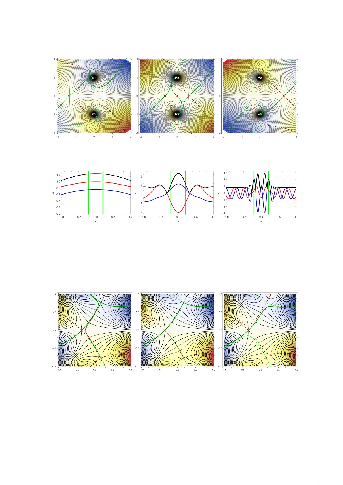
Prep ared for submission to JCAP Resurgence and Hyp erasymptotics in W ave Optics Astronomy Job F eldbrugge Samuel Crew Ue-Li Pen Higgs Cen tre for Theoretical Ph ysics, Univ ersit y of Edin burgh, James Clerk Maxw ell Build- ing, Edin burgh EH9 3FD, UK Departmen t of Ph ysics, National Tsing Hua Universit y , Hsinch u, T aiwan. Institute of Astronom y and Astroph ysics, Academia Sinica, Astronomy-Mathematics Build- ing, No. 1, Section 4, Ro osev elt Road, T aip ei 106319, T aiw an Canadian Institute for Theoretical Astrophysics, Universit y of T oronto, 60 St. George Street, T oronto, ON M5S 3H8, Canada P erimeter Institute for Theoretical Physics, 31 Caroline St. North, W aterlo o, ON, Canada N2L 2Y5 Departmen t of Physics, Univ ersit y of T oronto, 60 St. George Street, T oron to, ON M5S 1A7, Canada Dunlap Institute for Astronom y & Astroph ysics, Universit y of T oronto, 50 St. George Street, T oronto, ON M5S 3H4, Canada Canadian Institute for Adv anced Researc h, CIF AR program in Gravitation and Cosmology E-mail: job.feldbrugge@ed.ac.uk Abstract. With the disco very of gra vitational wa ves and fast radio bursts, w a v e optics has b ecome increasingly relev ant in astrophysics. This pap er studies the b eha viour of random gra vitational and plasma lenses, presenting the refractive and diffractiv e expansions, with higher-order terms that allow error estimates and embo dy the coun terin tuitiv e r esur genc e phenomenon. Sp ecifically , w e sho w that the diffractiv e expansion con v erges for a broad class of b ounded lens mo dels and provides an efficient description of in terference patterns across frequency regimes. Next, building on Picard–Lefschetz techniques, w e derive the full re- fractiv e expansion to arbitrary order, organising it into a transseries. Near caustics, the standard transseries is supplemented with uniform asymptotics. W e study this transseries, with b oth Borel and h yp erasymptotic resummation yielding systematic approximations to lensing integrals at all frequencies. Our results giv e a framework for modelling w a v e optics lensing near caustics and b ey ond the geometric optics approximation and thereby illustrate ho w to ols from resurgence and asymptotic analysis can be applied to practical problems in astroph ysics. Near caustic singularities, the p ost-refractive corrections diverge, while the uniform asymptotic expansion becomes accurate. W e use the leading uniform approximation to deriv e the strong w a v e optics suppression of off-axis caustics, which clarifies their sub dominan t role. Con ten ts 1 Introduction 1 2 The diffractive expansion 2 3 The refractive expansion 9 3.1 Classical rays and Picard-Lefschetz theory 9 3.1.1 Geometric optics 9 3.1.2 Picard-Lefsc hetz theory 11 3.1.3 The eikonal appro ximation 12 3.2 Laplace integrals 15 3.3 T ransseries 17 3.3.1 Non-degenerate ray 18 3.3.2 Caustics rays 21 4 Resurgence 25 4.1 The sup erasymptotic approximation 26 4.2 Borel resummation 27 4.3 The hyperasymptotic appro ximation 31 4.3.1 Ph ysical implications 36 5 Conclusion 37 A Algebraic curv es 42 1 In tro duction The theory and observ ation of gra vitational and plasma lensing pla y a cen tral role in mo dern astronom y . Historically , most studies ha v e relied on the geometric optics appro ximation, in whic h light is treated as ra ys following null geo desics in curved spacetime or as b eing deflected up on trav ersing a lens plane. While geometric optics remains adequate for most purp oses, w a v e optics has b ecome increasingly imp ortant with the adv en t of observ ations of gra vitational wa ves, fast radio bursts, and pulsars [ 1 – 3 ]. In these contexts—where coheren t, long-w a v elength radiation is lensed—the w a v e nature of ligh t can b e directly prob ed through observ able interference effects. This is especially relev ant near caustics, where the in tensity is amplified and the geometric optics approximation breaks do wn. The study of wa ve optics th us lies at the fertile intersection of caustics, singularity theory , and quantum interference. Although our presen t w ork centers on lens in tegrals, the results hold more general significance for the analysis of m ultidimensional oscillatory integrals. In particular, we an ticipate future applications to real-time F eynman path integrals. W av e effects in lensing constitute a ric h phenomenon that is notoriously challenging to mo del: the go v erning F resnel–Kirchhoff integrals are highly oscillatory , and their con vergence is delicate. This complexit y has historically restricted detailed calculations to the simplest case: lensing b y a single, isolated p oint mass [ 4 ]. Recen tly , t wo of the authors dev eloped an efficien t n umerical metho d based on the stationary-phase approach and Picard–Lefschetz – 1 – theory [ 5 ]. By deforming the original in tegration domain onto a set of complex Lefschetz thim bles—eac h asso ciated with a saddle p oin t and justified b y Cauch y’s theorem—the condi- tionally con v ergen t in tegral is transformed in to a sum of absolutely con v ergen t con tributions. This metho d has already enabled the syste matic study of several w a v e-optics lens mo dels [ 6 – 12 ]. In this paper, w e, for the first time, extend the analysis of w a v e optics in astrophysics to the analytical realm using r esur genc e the ory . In this pap er, we prov e that the diffr active exp ansion – normally developed in the diffractiv e regime – con verges for an y frequency and allows us to explore the full interference pattern and the caustics of the lens system in both the diffractive and refractive regimes without any kno wledge of classical rays. Next, we pro vide a new deriv ation of the r efr active exp ansion for d -dimensional lens integrals to arbitrary order, leading to an algorithm for its ev aluation. So far, studies of the refractive expansion hav e been limited to the eikonal appro ximation. How ever, the full refractive expansion of the Kirc hhoff-F resnel integral turns out to div erge, forming a transseries consisting of sev eral asymptotic series. Using the uni- form appr oximation, the sup er asymptotic and the hyp er asymptotic appr oximation techniques from resurgence theory , we show ho w to appro ximate the lens in tegral with differen t levels of precision using the formal refractive expansion. In particular, the hyperasymptotic appro xi- mation of the refractive expansion allo ws us to study the lens integral in b oth the refractiv e and diffractive regimes with arbitrary precision. Consequen tly , the diffractiv e and refractive expansions together form a pow erful analytic framew ork to model the lens integral for the full frequency range. While resurgence is a well-dev elop ed and sophisticated field of mathematics, this is the first application to lensing in wa ve optics. At presen t, most studies in resurgence either target specific mathematical aspects of the theory or are limited to one-dimensional integrals. In this pap er, we pro vide a p edagogical account of the use of resurgence theory to study ph ysical problems and, in the pro cess, deriv e several new results in resurgence relev an t to the ev aluation of multidimensional oscillatory in tegrals. The central mathematical points are demonstrated with a series of elementary examples. Outline. The pap er is structured as follo ws. W e b egin in section 2 with a discussion of the diffractive expansion. In section 3 , w e turn to the refractiv e expansion and derive the associated formal transseries that encodes the formal asymptotic approximation. In section 4 use resurgence theory to extract n umerical v alues for the lens integral using the transseries. W e conclude in section 5 with a discussion and outlo ok for future inv estigations. 2 The diffractive expansion In the present study , w e develop the diffractive expansion; the refractive expansion; and resurgence theory for the lensing of radiation b y a single thin lens. Let us consider a thin lens system, mo delled b y the dimensionless Kirchhoff-F resnel diffraction integral [ 13 , 14 ], Ψ( y ) =  ω 2 π i  d/ 2 Z e iω T ( x , y ) d x , (2.1) in terms of the dimensionless frequency ω ; the time delay T ( x , y ) = ( x − y ) 2 2 + φ ( x ) ; (2.2) – 2 – source RP observ er d l d sl L S ˆ x s ˆ y Figure 1 : The lens system displaying a ray moving from the angular p osition ˆ y on the source plane S to the angular p osition ˆ x on the lens plane L to the observer. the phase v ariation induced b y the lens φ and the dimension of the lens d . The mo dulus squared of the lens amplitude Ψ( y ) is interpreted as the intensit y I ( y ) = | Ψ( y ) | 2 at a p oin t y in the image plane (see fig. 1 for a diagram of the thin lens system with dimensional parameters.). The Kirchhoff-F resnel in tegral ranges o v er all possible rays moving from the source to the observer via the lens plane at p oin t x . F or conv enience, w e use dimensionless units with the dimensionless angular position on the lens plane x = ˆ x /θ ∗ , y = ˆ y /θ ∗ with some angular scale θ ∗ asso ciated with the lens system, and the dimensionless frequency ω = θ 2 ∗ d s cd sl d l ν with the angular frequency of the radiation ν . F or a detailed deriv ation of the Kirchhoff- F resnel in tegral from the real-time path in tegral, see [ 4 , 5 , 15 ] and we refer to [ 16 ] for a related deriv ation of gravitational lensing using relativistic world-line quan tisation. In the diffractive expansion, typically used in the diffractive regime ω ≪ 1, we expand the exp onen tial of the phase v ariation e iω φ ( x ) = ∞ X n =0 1 n ! [ iω φ ( x )] n , (2.3) and commute the infinite sum with the integration symbol to obtain the expansion Ψ( y ) =  ω 2 π i  d/ 2 Z e iω ( x − y ) 2 2 ∞ X n =0 1 n ! [ iω φ ( x )] n d x (2.4) ∼  ω 2 π i  d/ 2 ∞ X n =0 ω n n ! Z e iω ( x − y ) 2 2 [ iφ ( x )] n d x (2.5) = ∞ X n =0 a n ( y ) ω n , (2.6) with co efficien ts a n ( y ) =  ω 2 π i  d/ 2 1 n ! Z R d e iω ( x − y ) 2 2 [ iφ ( x )] n d x . (2.7) By construction, the first co efficien t a 0 = 1 while the subsequent co efficien ts a n are functions of the frequency . The diffractive expansion is t ypically used in the diffractive regime – for small frequencies ω – where the expansion typically conv erges rapidly to the lens amplitude. – 3 – Remark ably , the diffractiv e expansion ( 2.6 ) do es not necessarily conv erge as the lens in tegral conv erges only conditionally! 1 When moving the infinite sum outside the in tegration sym b ol, we are not, by the dominated conv ergence theorem, 2 guaran teed to recov er the lens in tegral. T o illustrate this phenomenon, let us study the diffractive expansion of a closely related integral. Example 1. Consider the one-dimensional quartic oscil latory inte gr al Φ = r ω π i Z ∞ −∞ e iω ( x 2 + x 4 ) d x (2.8) = r ω 4 π i e − iω 8 K 1 / 4  − iω 8  , (2.9) expr esse d in terms of the mo difie d Bessel function of the se c ond kind K n ( x ) . Exp anding e iω x 4 = P ∞ n =0 ( iω ) 2 n ! x 4 n and moving the sum outside the inte gr al yields the p ower series Φ ∼ r ω π i ∞ X n =0 ( iω ) n n ! Z ∞ −∞ e iω x 2 x 4 n d x = ∞ X n =0 (4 n − 1)!! 4 n n ! i n ω n , (2.10) with the double factorial n !! = n ( n − 2) · · · . The p artial sum Φ N = N X n =0 (4 n − 1)!! 4 n n ! i n ω n , (2.11) first appr o aches the value of the quartic inte gr al b efor e eventual ly diver ging (se e fig. 2 ). The terms in the exp ansion gr ow factorial ly with n . Note that after evaluating the c o efficients a n , the exp ansion or ganizes itself in inverse p owers of the fr e quency. Suc h a divergen t series appro ximation is referred to as an asymptotic series and o ccurs in man y physical problems. Consider, for example, the famous Dyson series in quantum electro dynamics or F eynman diagram expansions in quan tum field theory more generally . Dyson argued that if the p erturbative series in the electric charge e w ould con v erge for small e , it would define an analytic function in a small open disk | e 2 | < R in the complex plane, making the p ow er series also conv erge for e 2 < 0. Ho w ev er, this is unphysical as negative e 2 w ould render the v acuum unstable [ 17 ]. F rom the path integral persp ectiv e, the F eynman diagram expansion mirrors the diffractiv e expansion, and its asymptotic nature arises from mo ving an infinite sum outside of a conditionally conv ergent functional in tegral. Throughout history , asymptotic series intrigued and c hallenged some of the greatest mathematicians [ 18 ]. As w e will see in section 4 , in more recen t decades, the mathematical field of resurgence has dev elop ed a sophisticated understanding of asymptotic series and moreov er has dev elop ed 1 The integral R Ω f ( x )d x of the function f ov er the domain Ω conv erges absolutely when the integral o ver the modulus con verges i.e. , R Ω | f ( x ) | d x < ∞ . When the in tegral con v erges, but the in tegral ov er its mo dulus diverges, the integral is conditionally conv ergen t. The Kirc hhoff-F resnel integral is an example of a conditionally conv ergen t as the lens amplitude Ψ( y ) is finite but the integral ov er the modulus div erges, i.e. , R    e iωT ( x , y )    d x = R d x = ∞ . 2 The dominate d c onver genc e the orem: The limit of a set of integrals is guaran teed to conv erge to the in tegral of the limit when there exists a measurable function dominating the integrands of the sequence. Explicitly , lim n →∞ R f n ( x )d x = R lim n →∞ f n ( x )d x for sequence { f n } ∞ n =1 when there exists a function g such that R | g ( x ) | d x < ∞ and f n ( x ) < g ( x ) for all x and n . – 4 – (a) The real (red) and imaginary parts (blue) of the exact integral I (the lines) compared with the partial sum I N (the p oin ts). (b) The error of the partial sum I N with re- sp ect to the exact result I . Figure 2 : The partial sum I N of the asymptotic series of the in tegral compared with the closed form expression for I for ω = 10 as a function of the truncation p oin t N . concrete methods to extract from them increasingly accurate approximations of integrals and solution to differen tial equations. Ho w ev er, to our surprise, the diffractive expansion for the v ast ma jorit y of lens systems – despite relying on the exc hange of the sum and integration sym b ol for a conditionally con ver- gen t integral – does con verge to the Kirc hhoff-F resnel integral for an y frequency . Sp ecifically , when the in tegral o ver the phase-v ariation φ is in tegrable and bounded, the diffractiv e ex- pansion conv erges. T o see this, write φ as αϕ with α > 0 such that | ϕ ( x ) | < 1 for all x . The co efficien ts in the series expansion are b ounded by a rapidly decreasing function for large n , | a n ω n | =      ω 2 π i  d/ 2 ω n n ! Z e iω ( x − y ) 2 2 [ iφ ( x )] n d x     (2.12) ≤  ω 2 π  d/ 2 ( αω ) n n ! Z | ϕ ( x ) | n d x (2.13) ≤  ω 2 π  d/ 2 ( αω ) n n ! Ω , (2.14) as R | ϕ ( x ) | n d x ≤ R | ϕ ( x ) | d x = Ω since | ϕ ( x ) | < 1. Cauc h y’s ratio test 3 then guarantees the conv ergence of the diffractiv e expansion as the ratio of subsequen t terms in the series v anishes in the limit lim n →∞     a n +1 ω n +1 a n ω n     = lim n →∞ αω 2 n + 1 = 0 . (2.15) T o the b est of our kno wledge, the con v ergence of the diffractiv e expansion, irresp ectiv e of the frequency , for b ounded and in tegrable lenses is a new result. The diffractive expansion allo ws us to explore b oth the diffractiv e and the refractive regime in wa ve optics and analyse the nature of caustics and interference patterns without any knowledge of either real or complex classical ra ys! The natural speculation is that the asymptotic nature of F eynman diagram expansions results from the p olynomial nature of the interaction terms. 3 Cauchy’s ratio test: The series P ∞ n =1 a n con verges absolutely when the limit L = lim n →∞    a n +1 a n    con- v erges to a n umber L < 1. The series div erges when L > 1. When L = 1 or the limit fails to exist, the Cauc hy’s ratio test is inconclusive. – 5 – Figure 3 : The con v ergence of the diffractive expansion for the Lorentzian lens model at x = 0 for ω = 1 , 10 , 50 (blue, yello w, green). In terestingly , the diffractive expansion evolv es in precisely the opp osite manner to the asymptotic expansion. The terms a n ω n , scaling like ( α ω ) n n ! , first rapidly grow p eaking around n = ⌊ α ω ⌋ – the integer part of α ω – b efore decaying to zero (see fig. 3 ). As we will see, asymptotic series typically scale like n ! /F n for some constant F . F or small frequencies, the diffractiv e expansion is often highly efficient but in the large frequency regime, w e require man y terms to closely approximate the lens integral. Moreov er, the interference pattern emerges from the sum of increasingly large terms, requiring extremely precise ev aluations of the co efficien ts a n ( y ), making the expansion numerically unstable at high frequencies thereb y motiv ating the dev elopmen t of alternativ e metho ds for the high frequency regime (see section 3 and section 4 ). Nonetheless, the diffractive expansion pro vides a direct metho d for the ev aluation of lens integrals at any frequency using the Gaussian lens. F or general lens models, ev aluating the co efficien ts a n to the required accuracy is compu- tationally the most exp ensiv e step for ev aluating the diffractive expansion at high frequency . T o circumv en t this problem, let us consider the diffractiv e expansion for the Gaussian lens: Example 2. F or the Gaussian lens, the lens amplitude is Ψ( y ) =  ω 2 π i  d/ 2 Z e iω  ( x − y ) 2 2 + α exp [ − 1 2 ( x − µ ) T Σ − 1 ( x − µ ) ]  d x (2.16) =  ω 2 π i  d/ 2 ∞ X n =0 ( iω α ) n n ! Z e iω ( x − y ) 2 2 − n 2 ( x − µ ) T Σ − 1 ( x − µ ) d x (2.17) = ∞ X n =0 a n ( y ) ω n , (2.18) in terms of the amplitude α , the me an µ and the c ovarianc e Σ . The c o efficients of the diffr active exp ansion assume the form a n ( y ) = ( iα ) n n ! ( − iω ) d/ 2 p det( n Σ − 1 − iω I ) e − ω 2 2 ( y − µ ) T ( n Σ − 1 − iω I ) − 1 ( y − µ )+ iω ( y − µ ) 2 2 . (2.19) Giv en the closed-form expression for the co efficien ts a n , w e efficien tly ev aluate eac h term to the desired accuracy , ensuring the n umerical stability of the diffractive expansion in b oth – 6 – (a) ω = 50 (b) ω = 75 (c) ω = 100 Figure 4 : The interference pattern | I ( y ) = | Ψ( y ) | 2 for the one-dimensional Gaussian lens mo del with the parameters α = 2 , µ = 0, and σ = 1 ev aluated with Picard-Lefschetz theory (blac k) and the diffraction expansion (red) truncated at N = 550. (a) ω = 10 (b) ω = 20 (c) ω = 50 Figure 5 : The interference pattern I ( y ) = | Ψ( y ) | 2 for the t w o-dimensional Gaussian lens with the parameters α = 7, µ = 0 and Σ = diag(1 , 2) and the asso ciated caustics (the red curv es). (a) ω = 10 (b) ω = 20 (c) ω = 50 Figure 6 : The interference pattern I ( y ) = | Ψ( y ) | 2 for the phase-v ariation consisting of t w o Gaussian curv es φ ( x ) = 2 e − ( x 1 − 1) 2 + x 2 2 2 + 2 e − ( x 1 +1) 2 + x 2 2 2 with the asso ciated caustics (the red curv es). – 7 – the diffractive and refractive regimes. See figs. 4 and 5 for the resulting interference patterns of the one- and tw o-dimensional Gaussian lens in the refractive regime. The lens amplitude con v erges to the amplitude ev aluated with (Picard-Lefshetz numerical metho ds [ 5 ]). Next, we consider approximating an arbitrary b ounded and integrable one-dimensional lens mo del by a sum of Gaussian lenses, φ ( x ) ≈ N X r =1 α r φ r ( x − µ r ) , with φ r ( x ) = e − 1 2 x T Σ − 1 x , (2.20) for a set of amplitudes α r and p ositions µ r . F or a given phase v ariation φ , we can alwa ys ob- tain such an approximation by using radial interpolation to approximate the phase v ariation b y a sum of Gaussian curves [ 19 , 20 ]. Using the multinomial theorem [ φ 1 ( x ) + · · · + φ N ( x )] n = X k 1 + k 2 + ··· + k N = n  n k 1 , k 2 , . . . , k N  φ 1 ( x ) k 1 φ 2 ( x ) k 2 . . . φ r ( x ) k N , (2.21) with the m ultinomial  n k 1 ,...,k N  = n ! k 1 ! ...k N ! , w e obtain a diffractive expansion P ∞ n =0 a n ( y ) ω n with the co efficien ts a n ( y ) =  ω 2 π i  1 / 2 i n n ! X k 1 + k 2 + ··· + k N = n  n k 1 , k 2 , . . . , k N  α k 1 1 . . . α k N N × Z e iω ( x − y ) 2 2 e − 1 2 P N r =1 k r ( x − µ r ) T Σ − 1 ( x − µ r ) d x (2.22) =  ω 2 π i  1 / 2 i n n ! X k 1 + k 2 + ··· + k N = n  n k 1 , k 2 , . . . , k N  α k 1 1 . . . α k N N Z e iω ( x − y ) 2 2 e x T A x + B · x + C d x (2.23) = X k 1 + k 2 + ··· + k N = n i n α k 1 1 . . . α k N N k 1 ! k 2 ! · · · k N ! s − iω det ( − iω I − 2 A ) e 1 2 ( B − iω y ) T ( − iω I − 2 A ) − 1 ( B − iω y )+ iω y 2 2 (2.24) where the sum is taken ov er N p ositive integers k r ≥ 0 summing to n , with the constants A = − 1 2 N X r =0 k r Σ − 1 , B = Σ − 1 N X r =1 k r µ r ! , C = − 1 2 N X r =1 k r µ T r Σ − 1 µ r . (2.25) See fig. 6 for an illustration of the lens in tegral, obtained with this metho d, for a lens mo del with a phase-v ariation consisting of tw o Gaussian curves. The diffractive expansion of the Gaussian lens enables the analytic ev aluation of a large class of lens mo dels and do es not require any analytic prop erties of the phase v ariation mo d- els. Ho w ev er, for large frequencies and when summing man y Gaussian lenses, this calculation can become computationally expensive. Remark ably , the con vergence rate is not significantly influenced b y the dimensionalit y of the in tegral. As for high-dimensional Gaussian lenses and m ultidimensional lens problems, determining all the relev an t classical ra ys in the refractiv e appro ximation (discussed in section 3 ) can b e exp onen tially hard. The diffractiv e expansion pro vides an efficien t method to ev alaute the lens amplitude for these problems. The imple- men tation of this procedure for multiplane lens systems in wa ve optics and for F eynman path in tegrals will b e explored in a future pap er. – 8 – 3 The refractive expansion The diffractiv e expansion, t ypically used in the refractiv e regime ω ≫ 1, offers a conceptually transparen t method for appro ximating the lens in tegral that is particularly effectiv e in the lo w-frequency regime. The refractive expansion, discussed in the present section, pro vides a complemen tary persp ective that reveals the interpla y b et ween real and complex classical ra ys and their associated caustics. T raditionally , the refractive expansion is understoo d as the eikonal approximation in the large-frequency limit of the Kirchhoff-F resnel integral [ 15 ]. By employing the theory of resurgence we outline how classical rays and their associated div ergen t asymptotic series, assembled into a transseries, are intrinsically connected and enable the approximation of the lens integral to arbitrary accuracy at an y frequency . In principle, the refractiv e expansion can even b e extended to the diffractive regime! W e b egin with a concise review of the geometric optics approximation, Picard-Lefsc hetz theory and the eik onal appro ximation, emphasising their relationship to caustics. W e then mo v e beyond the eik onal regime to deriv e a transseries representation of the lens in tegral. W e dev elop the finite interpretation of the transseries through the framew ork of superasymptotic and hyperasymptotic appro ximations in resurgence theory in section 4 . 3.1 Classical ra ys and Picard-Lefsc hetz theory Lensing is t ypically introduced through the study of rays in the geometric optics appro xi- mation [ 15 , 21 ]. In this picture, radiation behav es like a classical pro jectile, deflected as it mo v es through the lens. Y et, remark ably , the concept of rays remains significant w ell b ey ond the geometric optics regime. 3.1.1 Geometric optics When the w av elength of the radiation is muc h smaller than the c haracteristic length scales of the lens, or the source emits incoherent radiation, wa ve effects can b e neglected, and the lens can b e accurately describ ed within the ge ometric optics appr oximation . F ollo wing F ermat’s principle, a classical ray is a stationary p oin t of the time delay function, i.e. , ∇ x T ( x , y ) = x − y + ∇ φ ( x ) = 0 . (3.1) Solving for y , we obtain the lens map ξ ( x ) = x + ∇ φ ( x ) . (3.2) A ra y in tersecting the lens at x is deflected by the angle ∇ φ ( x ) and forms an image at y = ξ ( x ). The intensit y follo ws from the con v ergence and divergence of a congruence of ra ys, I geometric ( y ) = X x ∈ ξ − 1 ( y ) 1 | det ∇ ξ ( x ) | . (3.3) The intensit y receives a con tribution from each real classical ray solving the equation ξ ( x ) = y . If a bundle of rays around a classical ra y spreads (con tracts), the determinant of the deformation tensor ∇ ξ is larger (smaller) than one and in tensit y receives a smaller (larger) con tribution from this particular ra y . When a point in the image plane y is reac hed b y m distinct ra ys – when y = ξ ( x ) has m real solutions – it is part of an m -image region. See fig. 7 – 9 – (a) ω = 1 (b) ω = 10 (c) ω = 50 Figure 7 : The geometric appro ximation I Geometric (red) and the lens integral | Ψ | 2 for the one- dimensional Loren tzian lens with amplitude α = 1 as a function of the frequency ω = 1 , 10 , and 50. for an illustration of the geometric optics approximation of the one-dimensional Loren tzian lens. The geometric optics approximation spik es in t w o, so-called, fold caustics separating t w o one-image regions from a three-image region in the middle. The intensit y spik es to infinit y when the determinan t of the deformation tensor ∇ ξ = I + H φ v anishes, with the Hessian of the phase-v ariation H φ . Such a point y c corresp onds to a degenerate critical p oin t x c of the time dela y for whic h both the gradien t ∇ x T ( x c , y c ) and the Hes sian H x T ( x c , y c ) is singular. Caustics come in a v ariety of morphologies that are famously classified b y catastrophe theory in terms of the elementary catastrophes [ 22 – 25 ]. An excellent and concise p edagogical introduction to catastrophe theory and its applications in the physical sciences can b e found in the textb o ok [ 26 ]. The m -image regions are b ounded b y the fold caustic ( A 2 ), defined b y the eigenv alue field of the deformation tensor λ i ( x ) = 0 , (3.4) for some i ∈ { 1 , 2 , . . . , d } , where the eigenv alue λ i and the eigenv ector v i of the deformation tensor are defined by the eigenequation ∇ ξ ( x ) v i ( x ) = λ i ( x ) v i ( x ) . (3.5) In terms of the eigenv alue fields, the intensit y is then giv en by I geometric ( y ) = X x ∈ ξ − 1 ( y ) 1 | λ 1 ( x ) | · · · | λ d ( x ) | . (3.6) In geometric optics, the fold caustics mark spik es in the intensit y pattern (see, for example, the green vertical lines in fig. 7 ). In wa ve optics, the fold caustics b ound the interference patterns (see, for example, the red curves in figs. 5 and 6 ). When, in addition, the fold curve is parallel to the eigenv ector field, v i ( x ) · ∇ λ i ( x ) = 0 , (3.7) the degenerate singularity forms a cusp caustic (for a deriv ation see, for example, [ 27 ]). The cusp ( A 3 ) caustics emerge as kinks in the fold caustic (as can b e seen in figs. 5 and 6 ). The fold and the cusp are the only caustics that form in generic t wo-dimensional lens problems. Oscillatory integrals with more external parameters can exhibit more complicated caustics, including the swallo wtail ( A 4 ), the butterfly ( A 5 ), the elliptic ( D + 4 ), the h yp erbolic ( D − 4 ) and the parab olic ( D 5 ) caustics. F or a detailed review of catastrophe theory and caustics in optics, we refer to [ 24 , 25 ]. F or an analysis of caustics in radio astronomy , see [ 28 ]. – 10 – 3.1.2 Picard-Lefsc hetz theory The classical rays not only go v ern the geometric optics appro ximation but are also key to understanding diffractiv e expansions of the lens amplitude through Pic ar d-L efschetz the ory [ 5 , 29 ]. The first in troduction of Picard-Lefschetz theory to theoretical ph ysics is found in [ 30 ] and for a pedagogical in tro duction and the first application to quan tum cosmology w e refer the reader to [ 29 ]. The Kirc hhoff-F resnel in tegral eq. ( 2.1 ) is highly oscillatory and conditionally conv ergent, making the definition delicate and the direct numerical ev aluation exp ensiv e [ 31 ]. Assuming the phase v ariation is a meromorphic function, w e may analytically con tin ue the time dela y in to the complex plane and deform the in tegration domain to impro v e the conv ergence properties of the integral. Cauch y’s in tegral theorem guarantees that the lens amplitude is preserv ed as long as w e k eep the endp oin ts (boundary of the in tegration domain) fixed, and we do not deform the in tegration contour past a singularity of the in tegrand. W riting the exp onen t in terms of a real and an imaginary part, iT ( x , y ) = h ( x , y ) + iH ( x , y ) , (3.8) w e note that the real part h = log | e iω T | go v erns the amplitude while the imaginary part H = arg( e iω T ) gov erns the oscillatory nature of the integrand. By flowing the original in tegration domain along the down w ard flow of the real part h , d γ λ ( x 0 ) d λ = −∇ h ( γ λ ( x 0 )) , (3.9) starting in γ λ =0 ( x 0 ) = x 0 and defining the gradient as one w ould on C d ≃ R 2 d , the integration domain is deformed in to the complex plane. Such a deformation preserv es the v alue of the in tegral while improving the con vergence prop erties of the in tegrand. In the limit λ → ∞ , the original in tegration domain transforms into a sum of steepest descen t manifolds 4 P j n j J j asso ciated to a set of real and complex classical ra ys x j – complex solution of of ξ ( x ) = y – forming the Picard-Lefsc hetz formula Ψ( y ) =  ω 2 π i  d/ 2 X j n j ( y ) Z J j e iω T ( x , y ) d x (3.10) =  ω 2 π i  d/ 2 X j n j ( y ) e iω H ( x j , y ) Z J j e ω h ( x , y ) d x . (3.11) The inclusion of complex solutions to the lens equation ξ ( x ) = y is cen tral to wa ve optics! The key insight of Picard and Lefschetz is that the steep est descent manifold J j , asso ciated with the classical ra y x j , is part of the deformation if and only if the asso ciated steep est as- cen t manifold 5 K j in tersects the original integration domain, n j = ⟨ R d , K j ⟩ ∈ Z (the brack et ⟨ J, K ⟩ v anishes when the manifolds J and K do not in tersect). When the steep est des cen t manifold of a classical ray x j is included, the classical ray is said to b e r elevant . When it is not part of the deformation, the classical ra y is irr elevant . Note that a real classical ray is alw a ys relev ant. The intersection num ber of a complex ray can b e ev aluated by studying the 4 The descent manifold J j of a classical ray x j consists of the p oin ts x 0 for which the do wnw ard flow γ λ ( x 0 ) reaches the classical ray x j in the limit of λ → −∞ . 5 The ascen t manifold K j of a classical ra y x j consists of the points x 0 for whic h the do wnw ard flo w γ λ ( x 0 ) reac hes the classical ra y x j in the limit λ → + ∞ . – 11 – descen t flow (for n umerical implemen tations see [ 5 , 32 ] and [ 33 ]). W e illustrate the Picard- Lefsc hetz deformation for the one-dimensional Lorentzian lens in fig. 8 . As the imaginary part H of the integrand is preserved by the down ward flow, 6 the Picard-Lefsc hetz deforma- tion resums the oscillations or the original integral and renders it absolutely con vergen t. In fact, one may argue that the original conditionally con v ergen t lens integral is ill-defined – its v alue depends on the c hosen regulator – and that the deformed in tegral eq. ( 3.11 ) constructed using analyticity is the proper rigorous definition (see [ 31 ] for a more detailed discussion). More practically , the Picard-Lefschetz deformation is the optimal deformation (among the con tours equiv alent to the original in tegration domain), cancelling all oscillations, and en- ables the efficien t n umerical ev aluation of the Kirc hhoff-F resnel integral [ 5 ]. See fig. 9 for the one-dimensional Loren tzian lens amplitude ev aluated with the Picard-Lefschetz numer- ical integration scheme. Below, w e verify the accuracy of the diffractiv e approximations by comparing the appro ximation with the numerically ev aluated lens amplitude. The Picard-Lefschetz deformation changes as a function of y . At a generic p oin t y , the c hange is smo oth. Ho w ev er, at a caustic and a Stok es transsition, the nature of the Picard-Lefsc hetz con tour changes dramatically . A t the caustics, where the time dela y has a degenerate critical p oint and tw o classical rays coalesce, the asso ciated steep est descent manifolds merge. After moving through the caustic, tw o of the coalescing rays b ecome complex classical rays forming a complex conjugate pair. One of these complex classical rays t ypically remains relev an t (the one for whic h h is negativ e) while the complex conjugate ra y is irrelev ant to the integral. A t a Stokes transition, where the steep est descent manifold of one classical ray x j terminates at another classical ra y x k , the relev ance of the classical ray x k c hanges (see fig. 10 ). As the gradien t descent preserv es the H -function, a Stok es transition where classical ra y x k c hanges relev ance is mark ed by H ( x j ) = H ( x k ) and h ( x j ) > h ( x k ). In fig. 11 , we outline the Picard-Lefsc hetz deformation for the Gaussian lens as a function of the p osition on the image plane y and the lens strength α . F or a more detailed discussion on Picard-Lefsc hetz theory in w a v e optics and the efficien t n umerical ev aluation of oscillatory in tegrals in the complex plane, we refer to [ 5 ]. 3.1.3 The eik onal appro ximation W e now turn to a brief review of the eikonal approximation. Upon expanding the time delay function in the Picard-Lefsc hetz formula for the in tegral o v er J j to quadratic order around the relev ant classical rays x j , T ( x , y ) ≈ T ( x j , y ) + 1 2 ( x − x j ) T [ H T ( x j , y )]( x − x j ) , (3.16) 6 W riting the p oin t on the lens plane and the path γ λ in terms of a real and an imaginary parts x = u + i v and γ λ = u λ + i v λ , satisfying the flo w equations d u λ d λ = −∇ u h and d v λ d λ = −∇ v h (with ∇ u and ∇ v the gradien t in the real and imaginary directions), w e find that d H ( γ λ ( x 0 )) d λ = ∇ u H · d u λ d λ + ∇ v H · d v λ d λ (3.12) = −∇ u H · ∇ u h − ∇ v H · ∇ v h (3.13) = −∇ h · ∇ H (3.14) = 0 , (3.15) b y the multidimensional Cauch y-Riemann equations ∇ h · ∇ H = 0. – 12 – (a) y = − 1 (b) y = 0 (c) y = 1 Figure 8 : Optimal deformation of the integration domain in the complex x -plane for the one-dimensional Lorentzian lens with amplitude α = 1. (a) ω = 1 (b) ω = 10 (c) ω = 50 Figure 9 : The diffraction integral of the one-dimensional Lorentzian lens with amplitude α = 1 ev aluated with Picard-Lefschetz theory . The red, blue and blac k curv es corresp ond to the real part, the imaginary part and the mo dulus of Ψ( y ) as a function of the frequency ω = 1 , 10 , and 50. The red lines mark the caustics. Figure 10 : In a Stok es transition (the cen tral panel), the steep est descen t of one of the com- plex rays terminates on another saddle p oin t. T o the left and right of the Stokes transition, the complex saddle point transitions from relev ant (the left panel) to irrelev an t (the righ t panel). – 13 – Figure 11 : Caustics (blac k) with the cusp (red) and Stok es lines (blue) in the y - α plane. the lens integral reduces to a set of Gaussian in tegrals. Ev aluating the Gaussian integrals leads to the eikonal approximation Ψ eikonal ( y ) = X j n j ( y ) e iω T ( x j , y ) p det ∇ ξ ( x j ) . (3.17) The eik onal approximation inherits the relev ance co efficient n j from the Picard-Lefschetz deformation discussed in the previous section. The relev ant branch of the square ro ot in the denominator follows from contin uity (starting, for example, from the free theory φ ( x ) = 0). Historically , the eik onal appro ximation is o ccasionally defined to only include real classic al ra ys, which are, by construction, all relev ant , i.e. , Ψ R eikonal ( y ) = X x ∈ ξ − 1 ( y ) e iω T ( x , y ) − im ( x ) π/ 2 p | det ∇ ξ ( x ) | . (3.18) In this real v ersion of the eikonal approximation Riemann sheet structure of the square ro ot is captured by the Morse-index m , given by the index of the classical ra y . F or t w o- dimensional lenses, the Morse-index is 0 , 1 , and 2 when the ra y x j is a minimum, a saddle p oin t and a maxim um of the time delay function T resp ectively . F or more details on the eik onal appro ximation, we refer to [ 15 , 25 ]. F or one of the first n umerical studies of the eik onal appro ximation of the Kichhoff-F resnel in tegral and its relation to caustics, w e refer to [ 28 ]. This appro ximation is arguably closer to the geometric optics appro ximation since squaring the amplitude | Ψ R eikonal | 2 and ignoring the cross terms w e recov er the geometric appro ximation ( 3.3 ). In figs. 12 and 13 we compare the full and real Eikonal appro ximation with the numerically ev aluated Kirchhoff-F resnel in tegral for the one-dimensional Lorentzian lens. The t w o approximations agree a w a y from the caustics where the contributions of complex rays are small. Both approximations diverge near the caustics, where det ∇ ξ = 0. Starting from the geometric optics appro ximation, the real eik onal approximation is the first step tow ards the wa v e nature in lensing. The full eikonal appro ximation, including – 14 – (a) ω = 1 (b) ω = 10 (c) ω = 50 Figure 12 : The real and complex eikonal approximation Ψ R eikonal (dotted) and Ψ eikonal (dashed) compared to the exact result (solid) for the one-dimensional Lorentzian lens with amplitude α = 1. The red and blue curv es corresp ond to the real and imaginary parts of the lens amplitude. The green lines mark the caustics. (a) ω = 1 (b) ω = 10 (c) ω = 50 Figure 13 : The difference b etw een the eikonal approximation and the exact result | Ψ( y ) − Ψ R eikonal ( y ) | (red) and | Ψ( y ) − Ψ eikonal ( y ) | (blue) for the one-dimensional Lorentzian lens with amplitude α = 1. The green lines mark the caustics. relev ant complex rays, is a significan t improv ement in the vicinity of caustics. In section 3.3 , w e demonstrate ho w to go beyond the eikonal approximation using the to ols of resurgence theory: uniform asymptotics, sup erasymptotics and hyperasymptotic expansions. 3.2 Laplace in tegrals In this section w e consider the Picard-Lefschetz formula for the Kirchhoff-F resnel in tegral from a different p ersp ectiv e. Let us, for conv enience, restrict the presen t discussion to the one- dimensional lens. At the end of this discussion, w e generalize to multidimensional integrals. Changing v ariables, t = − iT ( x, y ), the lens in tegral may b e in terpreted as a Laplace type in tegral Ψ( y ) = r ω 2 π i Z C y e − ω t ϕ y ( t )d t , (3.19) of the function ϕ y ( t ) =  d t d x  − 1 , (3.20) ev aluated ov er the integration domain C y = {− iT ( x, y ) | x ∈ R } . (3.21) – 15 – Note that the Jacobian ϕ y is obtained b y solving the p osition in the lens plane x as a function of t . This equation has generally multiple solutions, making the function ϕ y m ultiv alued. As will b e clarified in section 4.2 , the complex t -plane is kno wn as the Borel plane. Eac h saddle p oint x j of the original integral is transformed into a branch p oin t singularity of the integrand ϕ y at the point t j = − iT ( x j ) in the Borel plane. 7 The multiv alued nature of the Riemann surface ϕ y is a central feature of the lens in tegral considered as a Laplace-type in tegral. The integration con tour C y should b e in terpreted as a curve on the Riemann sheets of the Borel transform ϕ y , na vigating the branch p oin ts. See section A for a more detailed discussion on this algebraic curve/Riemann surface. The Laplace integral pro vides a p ow erful p erspective on the Picard-Lefschetz deforma- tion, as the descent flow preserves the imaginary part of the exp onen t. More sp ecifically , the original integration domain, the steepest ascen t and descent contours, transform in to line segmen ts C y , B J j and B K j in the Borel plane. The contour C y is a curve along the line Re[ t ] = 0 lo oping around the branc h p oin ts asso ciated with the real classical rays. The steep- est descent B J j and steep est ascen t con tours B K j in the Borel plane form horizontal lines, Im[ t ] = const, on the Riemann sheet. F or an illustration, we consider the Picard-Lefsc hetz deformation of the Lorentzian lens in b oth the complex x -plane and the Borel plane (see fig. 14 ). W e observe that the steep est ascent and descent manifolds simplify , while the orig- inal in tegration domain C y lo ops around the branc h cuts (flo wing around t 1 , t 2 and finally t 3 ). The relev ance of a saddle p oint can b e determined b y intersecting C y with B K j . A Stok es phenomenon corresp onds to the configuration where tw o branch points t j and t k ha v e the same imaginary part and “see” each other on the Riemann sheet in terms of the radar metho d of V oros [ 34 ] and Berry and Ho wls [ 35 ]. A t a Stokes transition, one branc h p oin t o v ertak es another branch p oin t in the Borel plane, i.e. , a Stokes transition o ccurs when the branc h points are on the same horizontal line Im t j = Im t k and are adjacent on the Riemann sheet. The Picard-Lefschetz formula leads to the expression Ψ( y ) = r ω 2 π i X j n j ( y ) e iω T ( x j ,y ) Z ∞ 0 e − ω t ∆ ϕ ( j ) y ( t )d t, (3.24) with ∆ ϕ ( j ) y the difference of ϕ j on the t w o Riemann shee ts ev aluated along the asso ciated horizon tal branch cuts in the Borel plane. As we will see in section 4.2 , the function ∆ ϕ y is kno wn as the Borel transform. 7 A nondegenerate critical point leads to a branc h p oin t of the form 1 / √ t , as can be seen from the Gaussian in tegral Z ∞ −∞ e iωx 2 d x = Z e − ωt d x d t d t = Z C e − ωt 1 + i 2 √ 2 t d t (3.22) with the con tour C in the Borel plane, running along the imaginary axes from + ∞ to the branc h point at t = 0 bac k to + ∞ at the other Riemann sheet of the square ro ot. Degenerate saddle p oints still map to singularity branc h p oin ts. How ever, the Riemann sheet structure at the branch p oint changes, as can b e observed from the integral Z ∞ −∞ e iωx n d x = Z C e − ωt e iπ 2 n nt 1 − 1 n d t . (3.23) – 16 – 5 4 3 2 1 2 1 0 1 2 2 1 0 1 2 Re( t ) Im( t ) 1 2 3 4 5 Figure 14 : The Picard-Lefschetz deformation for the one-dimensional Loren tzian lens with the parameters α = 2, y = 1 / 2. L eft: The complex x -plane with the classical rays p oints x j (the lab elled red p oin ts), the asso ciated steep est descen t J j (the green curves) and ascen t manifolds K j (the red curv es), and the optimal deformation of the real line (the dark green dashed curv es). Right: The asso ciated branc h p oin ts t j (the labelled red p oin ts), the steep est descen t B J j (the green curves) and ascen t manifolds B K j (the red curves) in the Borel plane around the branc h cuts (the grey zigzag lines). The original in tegration domain is mapp ed to the blue contour C y na vigating the branc h cuts. F or multidimensional integrals, the Borel transform is obtained by integrating ov er the lev el sets of the time delay restricted to a steep est descent manifold J j , ∆ ϕ ( j ) y ( t ) = Z { x ∈J j | T ( x , y )= t } d x ∥∇ x h ( x , y ) ∥ . (3.25) The multidimensional lens in tegral ev aluated along the steep est descent manifold J j of the classical ray x j assumes the form Ψ ( j ) ( y ) =  ω 2 π i  d/ 2 e iω T ( x j , y ) Z ∞ 0 e − ω t ∆ ϕ ( j ) y ( t )d t. (3.26) F or more details on the transformation to Laplace-t yp e in tegrals for multidimensional in te- grals, we refer to [ 36 ]. 3.3 T ransseries In this section, we pro ceed b eyond the eikonal approximation b y extending the seminal w ork of Dingle [ 37 ] to m ultidimensional integrals. Moreov er, we dev elop an algorithm to efficien tly compute the resulting transseries. W e first discuss the refractive expansion at nondegenerate classical rays, aw ay from a caustic, b efore showing how this result extends to caustics using uniform asymptotics. – 17 – 3.3.1 Non-degenerate ra y Starting from the Picard-Lefsc hetz formula ( 3.11 ), consider the Kirchhoff-F resnel integral along the steep est descen t manifold J j asso ciated with the nondegenerate saddle p oin t x j , Ψ ( j ) ( y ) =  ω 2 π i  d/ 2 Z J j e iω T ( x , y ) d x . (3.27) The T aylor series of the time dela y at x j is given by T ( x , y ) = T ( x j , y ) + 1 2 ( x − x j ) T [ H T ( x j , y )]( x − x j ) + X 3 ≤| α | ( x − x j ) α α ! ∂ α φ ( x j ) , (3.28) where w e use multi-index notation 8 α ∈ N d 0 . Expanding the exp onential of the third and higher order con tributions, we obtain the expansion Ψ ( j ) ( y ) =  ω 2 π i  d/ 2 e iω T ( x j , y ) Z J j e iω 2 ∆ x T [ H T ( x j , y )]∆ x ∞ X r =0 ( iω ) r r !   X 3 ≤| α | ∆ x α α ! ∂ α φ ( x j )   r d x , (3.29) with ∆ x = x − x j . Diagonalizing the Hessian H T = V Λ V − 1 with the eigenv alue matrix Λ = diag( λ 1 , . . . , λ d ) and the eigen v ector matrix V = ( v 1 , . . . , v d ), and rotating to the eigenframe of the Hessian b y setting ∆ x = V v (leading to the iden tit y ∆ x T [ H T ]∆ x = v T Λ v ), we use the multinomial expansion to write the p ow er of the sum as a multiv ariate p olynomial   X 3 ≤| α | ∆ x α α ! ∂ α φ ( x j )   r =   X 3 ≤| α | ( V v ) α α ! ∂ α φ ( x j )   r = X 3 r ≤| α | A r α v α . (3.30) The coefficients A r α are determined b y the m ultinomial theorem 9 and capture ho w the deriv a- tiv es of the phase v ariation enter the calculations that follow. Despite raising an infinite sum to a p o w er, each order of the resulting p olynomial consists of a finite set of terms. As w e will see b elo w, it is of crucial imp ortance that the sum starts at p olynomial order | α | = 3 r . Substituting this expansion into the lens integral, w e find Ψ ( j ) ( y ) ∼  ω 2 π i  d/ 2 e iω T ( x j , y ) ∞ X r =0 ( iω ) r r ! X 3 r ≤| α | A r α Z e iω 2 v T Λ v v α d v (3.32) = e iω T ( x j , y ) p det ∇ ξ ( x j ) ∞ X r =0 1 r ! X 3 r 2 ≤| β | i r + | β | (2 β − 1)!! λ β A r 2 β ω r −| β | , (3.33) 8 Giv en the multi-index α = ( α 1 , . . . , α d ) ∈ N d 0 , w e define its norm | α | = α 1 + · · · + α d , the first α ! = α 1 ! · · · α d ! and second factorial α !! = α 1 !! · · · α d !!, the p o w er x α = x α 1 1 · · · x α d d of a vector x = ( x 1 , . . . , x d ), and the partial deriv ative ∂ α = ∂ α 1 1 · · · ∂ α d d . 9 The multinomial theorem expresses the pow er of a sum as a sum of p o w ers, ( x 1 + x 2 + · · · + x m ) n = X k 1 + k 2 + · · · + k m = n k 1 , k 2 , · · · , k m ≥ 0 n k 1 , k 2 , . . . , k m ! x k 1 1 · x k 2 2 · · · x k m m . (3.31) – 18 – using the Gaussian identit y Z e iω 2 v T Λ v v α d v = (  2 π i ω  d/ 2 1 √ det Λ ( α − 1)!! λ α/ 2 ( − iω ) −| α | / 2 when α ∈ 2 N d 0 , 0 otherwise, (3.34) with the eigen v alue vector λ = ( λ 1 , . . . , λ d ). Up on ordering terms b y p o w ers of ω , we obtain the expansion Ψ ( j ) ( y ) ∼ e iω T ( x j , y ) p det ∇ ξ ( x j ) ∞ X m =0 T ( j ) m ( y ) ω m , (3.35) with the co efficien ts giv en by T ( j ) m ( y ) = 2 m X r =0 1 r ! X | β | = m + r i r + | β | (2 β − 1)!! λ β A r 2 β . (3.36) Eac h co efficient T ( n ) m consists of only a finite set of terms since the sum in eq. ( 3.30 ) starts at order | α | = 3 r . More sp ecifically , the co efficien ts T ( j ) 0 , T ( j ) 1 , . . . , T ( j ) M for a giv en order M , only dep end on the co efficients A r α for r ∈ { 0 , 1 , . . . , 2 M } and 2 M ≤ | α | ≤ 6 M . These co efficien ts A r α only dep end on the T a ylor series ( 3.28 ) to order | α | = 6 M . Using these insights, we may efficien tly ev aluate the first M co efficien ts T ( j ) m of the asymptotic expansion using algorithm 1 . Algorithm 1 Algorithm for the ev aluation of the co efficien ts T ( j ) m ( y ) of the asymptotic series. 1: Ev aluate the T a ylor series T ( x , y ) at the classical ray x j to order | α | = 6 M T ( x , y ) = T ( x j , y ) + 1 2 ( x − x j ) T [ H T ( x j , y )]( x − x j ) + X 3 ≤| α |≤ 6 M ( x − x j ) α α ! ∂ α φ ( x j ) , (3.37) with the Hessian H T ( x j , y ), its eigenv alues Λ and asso ciated eigenv ectors V . 2: Raise the truncated T aylor series to the p ow ers r = 0 , 1 , . . . , 2 M and extract co efficien ts A r α ,   X 3 ≤| α |≤ 6 M ( V v ) α α ! ∂ α φ ( x j )   r = X 3 r ≤| α |≤ 6 M r A r α v α . (3.38) F or an efficient implemen tation, we start with r = 0 and iden tify A 0 α = 1 when α = 0 and A 1 α = 0 when α  = 0. Multiply f = 1 with the sum, f ( v ) 7→ f ( v ) P 3 ≤| α |≤ 6 M ( V v ) α α ! ∂ α φ ( x j ) and read off the co efficients A 1 α . Rep eating this pro cess incremen tally builds up the co efficien ts A r α for r = 0 , 1 , . . . , 2 M . 3: Ev aluate the terms T ( j ) m ( y ) = 2 m X r =0 1 r ! X | β | = m + r i r + | β | (2 β − 1)!! λ β A r 2 β , (3.39) for m = 0 , 1 , . . . , M using the co efficien ts A r α obtained in step 2. – 19 – m T ( j ) m 0 1 1 5 F 2 3 − 3 F 2 F 4 24 F 3 2 2 385 F 4 3 − 630 F 2 F 4 F 2 3 +168 F 2 2 F 5 F 3 +3 F 2 2  35 F 2 4 − 8 F 2 F 6  1152 F 6 2 3 425425 F 6 3 − 1126125 F 2 F 4 F 4 3 +360360 F 2 2 F 5 F 3 3 − 10395 F 2 2  8 F 2 F 6 − 65 F 2 4  F 2 3 +3240 F 3 2 (4 F 2 F 7 − 77 F 4 F 5 ) F 3 − 27 F 3 2  1925 F 3 4 − 840 F 2 F 6 F 4 +8 F 2  5 F 2 F 8 − 63 F 2 5  414720 F 9 2 T able 1 : The first few terms of the asymptotic series T ( j ) m of the integral R e − ω f ( x ) d x with F i = ∂ n x f ( x j ) at the saddle p oint x j of f . T o the best of our kno wledge, this is the first closed-form expression and algorithm linking the deriv atives of the exponent at a nondegenerate saddle p oin t to the asso ciated series for multidimensional Laplace-type integrals. The formula extends the work by Dingle [ 37 ], who fo cused on the one-dimensional Laplace-type in tegral and computed the first term for tw o-dimensional in tegrals. Moreov er, algorithm 1 extends the more recen t analysis of one-dimensional Laplace-type integrals by [ 38 ]. In table 1 , we list the first few terms of the series expansion of the one-dimensional lens. The explicit expression of T ( j ) m in terms of the deriv atives of the time delay gro ws rapidly . Y et, the algorithm provides a straightforw ard metho d for the n umerical ev aluation of the co efficien ts. F or late terms, when the saddle p oin t x j is only known n umerically , the ev aluation requires arbitrary-precision floating-p oin t arithmetic to conv erge. W e find this metho d to b e more efficien t in practice than the contour in tegral metho ds prop osed in [ 35 – 37 ]. Substituting the expansion for Ψ ( j ) ( y ) in the Picard-Lefschetz form ula yields the transseries for the lens integral Ψ( y ) ∼ X j n j ( y )Ψ ( j ) ( y ) (3.40) = X j n j ( y ) e iω T ( x j , y ) p det ∇ ξ ( x j ) ∞ X m =0 T ( j ) m ( y ) ω m . (3.41) The transseries is a formal ob ject that bundles the saddle p oints, through exponential terms, together with their associated asymptotic series. T ransseries not only emerge in the study of integrals but also arise in the p erturbativ e study of differen tial equations (see, for example, [ 39 ]). W e calculate the transseries for the quartic integral: Example 3. The quartic inte gr al Φ = r ω π i Z ∞ −∞ e iω ( x 2 + x 4 ) d x, (3.42) has thr e e sadd le p oints lo c ate d along the imaginary axes x = 0 , x = ± i/ √ 2 . (3.43) T r acing the ste ep est desc ent c ontours, we find that only the r e al sadd le p oint is r elevant to the inte gr al (se e fig. 15 ). The series exp ansion ar ound the sadd le x = 0 c oincides with the diffr active exp ansion e q. ( 2.10 ) in example 1 and the series exp ansion at the sadd le p oints – 20 – Figure 15 : The Picard-Lefschetz deformation of the original in tegration domain of the in tegral R R e iω ( x 2 + x 4 ) d x in the complex x plane. The analytic con tin uation of the exponent has three saddle p oints (the red p oin ts) with the asso ciated steep est descent and ascent manifolds (the blue and red curves). The optimal deformation (the light green curve) of the original integration domain R (the dark green line). ± i/ √ 2 is given by r ω π i Z e ω ( − i/ 4 − 2 ix 2 ∓ 2 √ 2 x 3 + ix 4 ) d x = r ω π i e − iω 4 ∞ X n =0 ω n n ! Z ∞ −∞ e − 2 iω x 2 h ∓ 2 √ 2 x 3 + ix 4 i n d x = e − iω 4 √ 2 i  1 − 3 i 16 ω 2 + 15 i 8 ω 3 − 105 256 ω 4 + . . .  . (3.44) This le ads to the tr ansseries Φ ∼ n x =0 ∞ X n =0 (4 n − 1)!! 4 n n ! i n ω n +  n x = − i/ √ 2 + n x = i/ √ 2  e − iω 4 √ 2 i  1 − 3 i 16 ω 2 + 15 i 8 ω 3 − 105 256 ω 4 + . . .  , (3.45) with the interse ction numb ers n x =0 = 1 and n x = ± i/ √ 2 = 0 when starting with the inte gr al along the r e al line. T o zeroth order, the transseries reduces to the eikonal appro ximation as exp ected. Con- trary to what one ma y hop e, the sum P m =0 ∞ T ( j ) m /ω m div erges for eac h classical ra y (as w e already observ ed in example 1 ) since exchanging the infinite sum with the in tegration symbol in eq. ( 3.32 ) creates an asymptotic rather than a con vergen t series. In section 4 , we outline a rigorous interpretation of these divergen t transseries and discuss wa ys to approximate the lens integral to an arbitrary level of accuracy . 3.3.2 Caustics ra ys A t a caustic, b oth the eikonal and resurgence analysis (to b e discussed later in section 4 ) of the transseries break down since the determinan t of the deformation tensor v anishes. The time dela y function in the immediate vicinity of the caustic is no longer describ ed by the Hessian, and the deriv ation in section 3.3.1 does not apply . F ortunately , caustics are classified – 21 – Name Sym b ol Dimensionalit y Unfolding F old A 2 1D ψ ( t ) = 1 3 t 3 + µt Cusp A 3 2D ψ ( t ) = 1 4 t 4 + µ 2 2 t 2 + µ 1 t Sw allo wtail A 4 3D ψ ( t ) = 1 5 t 5 + µ 3 3 t 3 + µ 2 2 t 2 + µ 1 t Butterfly A 5 4D ψ ( t ) = 1 6 t 6 + µ 4 4 t 4 + µ 3 3 t 3 + µ 2 2 t 2 + µ 1 t Elliptic umbilic D − 4 3D ψ ( t ) = t 3 1 − 3 t 1 t 2 2 − µ 3 ( t 2 1 + t 2 2 ) − µ 2 t 2 − µ 1 t 1 Hyp erbolic umbilic D + 4 3D ψ ( t ) = t 3 1 + t 3 2 − µ 3 t 1 t 2 − µ 2 t 2 − µ 1 x 1 P arab olic um bilic D 5 4D ψ ( t ) = t 4 1 + t 1 t 2 2 + µ 4 t 2 2 + µ 3 x 2 1 + µ 2 t 2 + µ 1 t 1 T able 2 : The unfoldings ψ of the elementary catastrophes, with the intrinsic v ariables lab elled b y t and the external parameters lab elled b y µ . in terms of the elemen tary catastrophes and can be treated separately . The sev en elemen tary catastrophes form a complete classification of degenerate critical p oin ts up to four external parameters. In table 2 we list the first sev en elementary catastrophes and their unfolding, describing their canonical b eha viour. F or a review on catastrophe theory more generally , see [ 23 , 26 ]. W e will derive the uniform asymptotic expansion of the fold caustic here. The higher-order caustics follo w analogously . F or more details on uniform asymptotic asymptotics w e refer to [ 40 – 49 ]. F or a first-order application of uniform asymptotics to w a v e optics in astronom y , see [ 50 ]. F or conv enience, we will first consider the one-dimensional lens problem. In the follow- ing, w e will only consider the transseries contributions of the rays in v olv ed in the caustic. When x c is a fold catastrophe, mapp ed to the fold caustic at y c in the image plane, b oth its first- and second-order deriv atives v anish, i.e. , the point ( x c , y c ) is a real solution of the equations ∂ x T ( x c , y c ) = x c − y c + φ ′ ( x c ) = 0 , (3.46) ∂ 2 x T ( x c , y c ) = 1 + φ ′′ ( x c ) 2 = 0 . (3.47) The T aylor expansion of the time dela y function at the fold caustic then assumes the form T ( x, y ) = T ( x c , y ) − ∆ y ∆ x + ∞ X n =3 φ ( n ) ( x c ) n ! ∆ x n , (3.48) with x − x c = ∆ x and y − y c = ∆ y . The lens integral, Ψ( y ) = r ω 2 π i e iω T ( x c ,y ) Z e iω  − ∆ y ∆ x + P ∞ n =3 φ ( n ) ( x c ) n ! ∆ x n  d∆ x , (3.49) simplifies using the co ordinate transformation ∆ x = 3 q 2 φ (3) ( x c ) t to an expansion in terms of the canonical form of the fold catastrophe, Ψ( y ) ∼ r ω 2 π i 3 s 2 φ (3) ( x c ) e iω T ( x c ,y ) Z e iω ( 1 3 t 3 + µt + P ∞ n =4 B n n ! t n ) d t (3.50) = r ω 2 π i 3 s 2 φ (3) ( x c ) e iω T ( x c ,y ) Z e iω ( 1 3 t 3 + µt ) ∞ X r =0 ( iω ) r r ! " ∞ X n =4 B n n ! t n # r d t , (3.51) – 22 – with µ = − 3 s 2 φ (3) ( x c ) ∆ y , B n = φ ( n ) ( x c )  2 φ (3) ( x c )  n/ 3 . (3.52) Expanding the p ow er of the sum, " ∞ X n =4 B n n ! t n # r = ∞ X p =4 r A r p t p , (3.53) w e obtain the series Ψ( y ) ∼ r ω 2 π i 3 s 2 φ (3) ( x c ) e iω T ( x c ,y ) ∞ X r =0 ( iω ) r r ! ∞ X p =4 r A r p Z e iω ( 1 3 t 3 + µt ) t p d t . (3.54) This expansion can then b e expressed in terms of Airy functions as Z e iω ( 1 3 t 3 + µt ) t p d t = 2 π i p ω ( p +1) / 3 Ai ( p ) ( ω 2 / 3 µ ) , (3.55) where Ai ( p ) ( x ) denotes the p th-order deriv ative of the Airy function. W orking in terms of the external parameter ˜ µ = ω 2 / 3 µ , the uniform as ymptotic expansion assumes the form Ψ( y ) ∼ r ω 2 π i 3 s 2 φ (3) ( x c ) e iω T ( x c ,y ) ∞ X m =0 T m ω m/ 3 , (3.56) with T m = m − 1 X r =0 2 π i − 2 r − m +1 A r 3 r + m − 1 r ! Ai (3 r + m − 1) ( ˜ µ ) . (3.57) Using the iden tity Ai ′′ ( x ) = x Ai( x ), we can express the p th-order deriv ative in terms of the Airy function and its first-order deriv ativ e (for a closed-form expansion see [ 51 ]). This leads to a formulation of the uniform expansion of the fold caustic in terms of the Airy function and its first-order deriv ativ e, Ψ( y ) ∼ √ − 2 π iω 3 s 2 φ (3) ( x c ) e iω T ( x c ,y ) " Ai( ˜ µ ) ∞ X n =1 a n ω n/ 3 + Ai ′ ( ˜ µ ) ∞ X n =1 b n ω n/ 3 # . (3.58) In table 3 we presen t explicit expressions for the first few terms in the asymptotic expan- sion. As for the transseries obtained in section 3.3.1 , the asymptotic series of the uniform asymptotic expansion first conv erges b efore even tually div erging. Near higher-order caustics, an analogous uniform asymptotic expansion follo ws in terms of a set of canonical diffraction in tegrals R e iψ ( t ) d t with the associated unfolding ψ ( t ) (see table 2 ) of the catastrophe in question [ 52 ]. F or the cusp caustic, this integral is related to the famous Pearcey in tegral [ 53 ]. Practically , the efficien t ev aluation of the co efficien ts follows algorithm 1 . – 23 – (a) ω = 1 (b) ω = 10 (c) ω = 50 Figure 16 : The difference b et w een the exact lens integral and the leading uniform approx- imation | Ψ( y ) − Ψ uniform ( y ) | (red) and the eik onal appro ximation | Ψ( y ) − Ψ eikonal ( y ) | (blue) for the one-dimensional Lorentzian lens with amplitude α = 1. The green lines mark the caustics. T o leading order, the uniform approximation is given by Ψ uniform ( y ) = √ − 2 π i 3 s 2 φ (3) ( x c ) e iω T ( x c ,y ) ω 1 / 6 Ai( ω 2 / 3 µ ) . (3.59) See figs. 16 and 17 for a numerical demonstration of the zeroth-order uniform approximation of the one-dimensional Loren tzian lens mo del. Awa y from the caustics, the standard eik onal appro ximation provides a more accurate description than the uniform appro ximation. In the vicinity of the caustics, how ev er, the uniform approximation smo othly approaches the lensing amplitude and regularises the divergence inherent in the eikonal approximation. As w e increase the frequency , the region around the caustics for which the uniform approximation is b eneficial shrinks. The uniform approximation works b est in the refractive regime. In the diffractiv e regime, the uniform approximation starts to deviate from the true lens amplitude. T o impro v e the conv ergence prop erties of the transseries ( 3.41 ) near the caustics, we replace the terms asso ciated with the caustic with the asso ciated uniform asymptotic formula. The application of the uniform approximation near the fold caustics in astrophysi- cal lensing w as recently in tro duced b y [ 50 ]. How ever, their treatment differs significantly from the present discussion in several resp ects. Firstly , they fo cus on the leading con- tribution and do not consider the full asymptotic series. Secondly , using the form Ψ = √ 2 π e iχ [ g 1 Ai( ζ ) + g 2 Ai ′ ( η )] they approximate the functions g 1 , g 2 , χ and ζ from the geomet- ric optics approximation rather than from an expansion of the time dela y function at the fold caustic. Consequen tly , their treatmen t neatly extends the eikonal appro ximation to the fold caustics, but do es not relate it directly to the T a ylor series of the time delay at the fold caustic. A typical caustic is crossed in the o verfocussed regime, corresp onding to large α . The asymptotic p eak intensit y of this image is I = I 0 ω 1 / 3 with I 0 = 2 1 / 3 16 π 27(3 α ) 2 / 3 Γ[2 / 3] 2 and I ∼ 0 . 61( ω /α 2 ) 1 / 3 . F or off axis lenses, the peak caustic flux is small. In t ypical ESE scenarios (where α is called conv ergence κ in [ 54 ]), κ ∼ 20, ω ∼ 40, the p eak caustic flux is only 30% of the unlensed flux, consistent with the lack of salient caustic p eaks in secondary wa vefields. The av erage geometric optics lensed image flux is ∝ 1 /κ , leading to a mo deset fractional caustic enhancement ∝ ( ω κ ) 1 / 3 . F or multidimensional in tegrals, the asymptotic series follows from a combination of the deriv ation of the degenerate and non-degenerate expansions. F or example, for a fold caustic – 24 – (a) The lens amplitude (b) The in tensity Figure 17 : The lens amplitude and in tensit y of the one-dimenisonal Loren tzian lens with α = 1 at the fold caustic and the uniform approximation as a function of frequency . Left: The real (red) and imaginary parts (blue) of the lens amplitude. The solid curves show the true amplitude and the dashed curves show the leading uniform approximation. Right: The in tensit y of the lens (blac k) and the leading uniform approximation (dashed red). n a n b n 1 1 0 2 iB 4 ˜ µ 2 24 iB 4 12 3 B 5 ˜ µ 30 − B 2 4 ˜ µ ( ˜ µ 3 +28 ) 1152 ( 4 B 5 − 5 B 2 4 ) ˜ µ 2 480 4 − i ( − 576 B 5 B 4 ( 4 ˜ µ 3 +7 ) +576 B 6 ( ˜ µ 3 +4 ) +5 B 3 4 ( ˜ µ 6 +260 ˜ µ 3 +280 )) 414720 − i ˜ µ ( 25 B 3 4 ( ˜ µ 3 +20 ) − 24 B 5 B 4 ( ˜ µ 3 +52 ) +576 B 6 ) 69120 T able 3 : The first terms in the asymptotic series of the uniform asymptotic expansion of a fold caustic. in a tw o-dimensional lens integral, for which one of the eigenv alues of the deformation tensor v anishes, there exists a co ordinate system in which the time delay takes the form T ( x , y ) ≈ T ( x c , y ) + 1 3 ∆ x 3 1 + µ ( y )∆ x 1 + ∆ x 2 2 (3.60) to leading order. Up on expanding the exp onential of the higher-order terms, the in tegrals in the expansion factorise. The integral ov er x 1 follo ws the deriv ation of the fold caustic, while the integral ov er x 2 follo ws the deriv ation of the non-degenerate saddle p oint. 4 Resurgence In section 3.3 , we extended the eik onal appro ximation to the transseries expansion. A t first glance, this app ears to offer little improv ement, since eac h series asso ciated with a classical ray is asymptotic and divergen t! In contrast to the diffractive expansion, the formal transseries do es therefore naively fail to appro ximate the lens integral. This puzzling b eha viour histor- ically confounded sev eral eminent mathematicians – among them Niels Ab el, who famously remark ed that “divergen t series are the in v en tion of the devil, and it is shameful to base on them an y demonstration whatsoever.” Bay es claimed that Stirling’s series, whic h is indeed – 25 – asymptotic, “can never properly express any quan tity at all” and the metho ds used to obtain it “are not to b e dep ended up on.” Y et, ov er the past century , the pioneering work of Borel, Dingle, ´ Ecalle, and later Berry , Ho wls, and Olde Daalh uis ha ve provided a rigorous frame- w ork for the analysis of asymptotic series, known as the theory of resurgence [ 35 – 37 , 55 – 60 ]. Their contributions reveal ho w transseries can b e resummed, yielding exp onentially accurate appro ximations to the underlying in tegrals or, more generally , solutions to differen tial equa- tions. Interestingly , while the diffractiv e expansion first div erges b efore con v erging to the lens amplitude, the refractive appro ximation – through resurgence on the formal transseries – can b e made to conv erge more quickly and un veils the analytic structure of the in terference pattern. In this section, we discuss the sup erasymptotic approximation, Borel resummation and ultimately the hyperasymptotic approximation that allo ws us to extract finite results for the lens amplitude from a formal transseries. 4.1 The sup erasymptotic appro ximation The superasymptotic appro ximation is the most direct and practical w a y to work with the transseries and it has a rich history going bac k to w ork b y P oincar´ e, Stieltjes, Cauc hy and Stok es. The sup erasymptotic metho d w as formalised b y Berry and Howls [ 56 ]. As illustrated in example 1 , an asymptotic series typically approaches the true result b efore ev en tually div erging. The reason underlying this b ehaviour will become clear in section 4.3 . It is th us natural to truncate the sum P ∞ m =0 T ( j ) m /ω m at the index for which | T ( j ) m /ω m | is the smallest, denoted as N ( j ) . This leads to the sup erasymptotic appro ximation Ψ super ( y ) = X j n j ( y ) e iω T ( x j , y ) p det ∇ ξ ( x j ) N ( j ) X m =0 T ( j ) m ( y ) ω m . (4.1) As we will discuss in section 4.3 , the optimal truncation p oin t N ( j ) is prop ortional to the difference of the time dela y in the ray x j and the closest classical ra y in the Borel plane. More explicitly , defining the so-called singulant F j k = i ( T ( x j , y ) − T ( x k , y )) . (4.2) the optimal truncation p oint N ( j ) is the integer part of | ωF j k ∗ | with k ∗ the lab el of the ray x k ∗ that lives on the same Riemann sheet and is closest to x j in the Borel plane, i.e. the ray on the same Riemann sheet in the Borel plane for which the mo dulus of the singulant | F j k | is the smallest. The error in the sup erasymptotic appro ximation is of the order e −| ω F j k ∗ | . The sup erasymptotic approximation provides a natural refinement of the eikonal ap- pro ximation. W e compare the error of the eikonal and the superasymptotic approximation of the one-dimenisonal Lorentzian lens as a function of space y and frequency ω in fig. 18 . Awa y from the caustics, the sup erasymptotic appro ximation pro vides a significan t increase in ac- curacy . In the one-dimensional Lorentzian lens example, the sup erasymptotic appro ximation reac hes the accuracy lev el with whic h we numerically ev aluate the integral with a Picard- Lefsc hetz in tegrator for | y | ≥ 0 . 8 (see section 3.1.2 ). Near the caustics, where | ω F j k ∗ | drops b elo w unity , the superasymptotic appro ximation coincides with the eik onal approximation. In these regions the asymptotic series directly div erges. The same phenomena are observ ed in the frequency domain. F or large frequencies, the sup erasymptotic approximation is a signifi- can t impro v emen t o v er the eik onal approximation. F or small frequencies, when | ω F j k ∗ | drops b elo w unity , the superasymptotic appro ximation coincides with the eik onal approximation. – 26 – (a) The error as a function of space (b) The error as a function of frequency Figure 18 : L eft: The mo dulus of the lens amplitude (blac k), eik onal approximation (blue), and sup erasymptotic approximation (green), and first-order hyperasymptotic approximation (blac k) of the one-dimensional Lorentzian lens as a function of the frequency with the am- plitude α = 1 and the p oint on the sky y = 0 . 3 as a function of the frequency . Right: The asso ciated error with resp ect to the eik onal appro ximation | Ψ − Ψ eikonal | (blue), the sup erasymptotic appro ximation | Ψ − Ψ super | (green) and first-order hyperasymptotic approx- imation | Ψ − Ψ hyper | (red). Near caustics, the transseries obtained from the expansion around nondegenerate rays fails. As we observed in section 3.3.2 , in these regions the sup erasymptotic approximation of the uniform asymptotic expansion provides a significantly b etter approximation. 4.2 Borel resummation A t first sight, the sup erasymptotic approximation app ears to encounter an imp enetrable barrier. W e leveraged the conv ergent part of each asymptotic expansion and are left with a div ergen t tail! Y et, the divergen t tail turns out to encode the full analytic structure of the oscillatory in tegral (this idea was first realized by Dingle [ 37 ]). T o understand this in detail, w e will first show ho w the formalism of Borel resummation can, in principle, recov er the lens in tegral [ 61 ]. In section 4.3 , we use hyperasymptotics to approximate the lens in tegral to arbitrary precision b eyond the sup erasymptotic approximation. Starting with the transseries, Ψ( y ) ∼ X j n j ( y ) e iω T ( x j , y ) p det ∇ ξ ( x j ) ∞ X m =0 T ( j ) m ( y ) ω m , (4.3) w e Borel resum the asymptotic series T ( j ) y ( ω ) = P ∞ m =0 T ( j ) m ( y ) /ω m for each classical ra y with the following scheme: 1. W e first define the Borel transform by dividing each term by a factorial B T ( j ) y ( t ) = ∞ X m =0 T ( j ) m ( y ) m ! t m . (4.4) The series P ∞ m =0 T ( j ) m /ω m is said to be Borel summable when the Borel transform B T ( j ) y con v erges. Asymptotic series originating from Laplace-type integrals generally diverge factorially , making the Borel transform conv erge. – 27 – 2. Next, we Laplace transform the Borel transform to obtain the so-called Borel sum of the asymptotic series T ( j ) B ( y ) = ω Z ∞ 0 e − ω t B T ( j ) ( t )d t . (4.5) No w, rather surprisingly , replacing the asymptotic series P ∞ m =0 T ( j ) m /ω m with the Borel re- summed series T ( j ) B yields the full lens amplitude Ψ( y ) = X j n j ( y ) e iω T ( x j , y ) p det ∇ ξ ( x j ) T ( j ) B ( y ) . (4.6) The Borel resummation metho d has conv erged the formal transseries into the lens amplitude, irresp ectiv e of the frequency . W e illustrate Borel resummation for the asymptotic series of the quartic in tegral. Example 4. In examples 1 and 3 , we derive d that the diffr active exp ansion of the quartic inte gr al le ads to the asymptotic series Ψ = r ω 2 π i Z ∞ −∞ e iω ( x 2 + x 4 ) d x ∼ ∞ X n =0 (4 n − 1)!! 4 n n ! i n ω n . (4.7) L et us Bor el r esum this diver gent series and c omp ar e it with the close d form expr ession pr esente d in example 1 . The series diver ges factorial ly, and the Bor el tr ansform c onver ges B Ψ( t ) = ∞ X n =0 (4 n − 1)!! 4 n ( n !) 2 i n t n (4.8) = 2 π 4 √ 1 + 4 it K  1 2 − 1 2 √ 4 it + 1  (4.9) in terms of the c omplete el liptic inte gr al of the first kind K ( m ) . The L aplac e tr ansform r e c overs the original inte gr al ω Z ∞ 0 e − ω t B I ( t )d t = r ω 4 π i e − iω 8 K 1 / 4  − iω 8  , (4.10) wher e K n ( x ) denotes the mo difie d Bessel function of the se c ond kind. We have thus evaluate d the quartic inte gr al by me ans of Bor el r esummation using the close d form r epr esentation of the Bor el tr ansform. Let us no w make some informal observ ations: • At first sigh t, Borel resummation is a remark able pro cedure. W e artificially introduce a factorial suppression and subsequen tly ‘integrated it out’. The central idea b eing that the Laplace transform of the monomial factor leads to a multiplication by the same factorial factor Z ∞ 0 e − t t n = n ! . (4.11) Indeed, when a series P ∞ n =0 a n con v erges absolutely – that is to say P ∞ n =0 | a n | < ∞ – w e can c hange the order of summation and in tegration. Moving the Laplace in tegral inside the sum, the Laplace integral cancels the factorial in the Borel transform. Consequently , Borel resummation on an absolutely conv ergent series recov ers the original series. – 28 – • On the other hand, when truncating the sum in the Borel transform, the Laplace transform reco vers the original series irrespective of whether it conv erges or div erges. Ha ving complete kno wledge of the transseries and performing the infinite sum in the Borel transform b efore the Laplace transform is critical. • In general – when the sum do es not con v erge absolutely – exc hanging the in tegration sym b ol with the infinite sum is not admissible. The order of op erations matters. In a lo ose sense, the div ergence in eq. ( 4.3 ) arose from mo ving the infinite sum outside the in tegral, ignoring the conditions of the dominated con vergence theorem. The original in tegral is reco vered by inserting the factorial and ‘cancelling’ this step with the Laplace transform! The question we now turn to is what properties, in these cases, guaran te e con v ergence to the original in tegral? T o understand the idea underlying Borel resummation, we note that eac h analytic func- tion f ( ϵ ) has a unique expansion f ( ϵ ) = ∞ X n =0 f n ϵ n (4.12) in the small parameter ϵ . The conv erse is generally not true, as the function g ( ϵ ) = f ( ϵ ) + e − 1 /ϵ (4.13) is distinct, but has an identical expansion. 10 The series expansion can serv e as a fingerprint of an analytic function, but is generally not unique. Under a set of mild conditions, W at- son’s theorem, whic h is a c onsequence of analyticit y , and its generalisations guarantee that the mapping becomes one-to-one. 11 W e conclude that an asymptotic series resulting from 10 This is a consequence of the observ ation that any deriv ativ e of the exp onential e − 1 /ϵ v anishes at ϵ = 0. 11 W atson’s theorem was the first attempt to build a one-to-one corresp ondence betw een analytic functions and their expansions [ 62 ]. F. Nev anlinna [ 63 ] and later Sok al [ 64 ] extended W atson’s theorem to a more general class of analytic functions. Also, see [ 65 ] for an extension of this w ork. • When the function f is analytic in a circle C R of radius R centred at R in the complex ϵ plane, and when in addition the residue of the partial sum R N ( z ) defined b y f ( ϵ ) = N − 1 X n =0 f n ϵ n + R N ( ϵ ) (4.14) is b ounded b y | R N ( ϵ ) | ≤ Aσ N N ! | ϵ | N (4.15) for some p ositiv e A and σ , the Borel transform ϕ ( t ) = P ∞ n =0 f n t n /n ! con v erges along a region around the p ositive real half line, and the function f can b e written as the Laplace transform f ( ϵ ) = 1 ϵ Z ∞ 0 e − t/ϵ ϕ ( t )d t , (4.16) for z ∈ C R . In our context ϵ = 1 /ω . • Conv ersely , when we can write the function f as a Laplace type integral ( 4.16 ) with the function ϕ analytic in a neighbourho o d of the p ositiv e real half-line, and moreov er, | ϕ ( t ) | ≤ K e | t | /R (4.17) for some K in this region, the expansion of the function f ( ϵ ) obtained from f n = ϕ ( n ) ( t ) | t =0 satisfies the prop erty ( 4.15 ). – 29 – the Kirchhoff-F resnel integral is Borel resumable as we can write it as Laplace-t yp e integral. Since the original in tegral and the Borel resummed expression share the same expansion and are b oth of Laplace t yp e, the resummed expression needs to coincide with the original lens in tegral and the full information of the lens integral b ey ond the sup erasymptotic approxima- tion is enco ded in the div erging tails of the asymptotic series of the transseries! It turns out that Borel resummation is indeed one metho d among a large class of resummation metho ds, constructing a con v ergen t expression with the s ame asymptotic expansion, and lev eraging the corresp ondence b etw een analytic functions and their asymptotic series (see, for another prominen t example, Mittag-Leffler summation [ 66 ]). F or an insigh tful review and further details, we refer the reader to [ 18 ]. In section 3.2 , we changed coordinates and rewrote the Kirchhoff-F resnel integral as the Laplace type integral of the algebraic curve ϕ y ( t ). The discussion ab ov e indicates that ∆ ϕ ( j ) y ma y b e interpreted as the Borel transform, i.e. , ∆ ϕ ( j ) y ( t ) = ∞ X m =0 T ( j ) m ( y ) m ! t m . (4.18) In practice, one can therefore either Borel transform the asymptotic series or p erform the c hange of co ordinates on the integral. Another alternative is to derive the asymptotic series from the algebraic curv e asso ciated to the Borel transform by expanding around the branc h p oin ts (see section A for further details on this approac h). In the Laplace represen tation, the function ϕ y ( t ) = ( dt/dx ) − 1 is m ulti-v alued because the equation t = − iT ( x, y ) has m ultiple lo cal inv erses. Hence ϕ y defines a Riemann surface o v er the t -plane with branch points at t j = − iT ( x j , y ). F or the contribution of a fixed saddle x j , the map t = − iT sends the steep est descent contour J j to a branch cut b eginning from t j , and the integral along J j b ecomes an integral of the discontin uit y across that cut, ∆ ϕ ( j ) y ( t ) := ϕ (+) y ,j ( t ) − ϕ ( − ) y ,j ( t ) , (4.19) where ± denote b oundary v alues on the t w o sides of the cut. Near a saddle p oin t, the lo cal b eha viour is ∆ ϕ ( j ) y ( t ) = (2 π i ) d/ 2 Γ( d/ 2) t d 2 − 1 p det ∇ ξ ( x j ) (1 + O ( t )) . (4.20) Defining U ( j ) y ( ω ) := ω d/ 2 Z ∞ 0 e ω t ∆ ϕ ( j ) y ( t ) dt, (4.21) and comparing with the Borel expansion Ψ ( j ) ( y ) ∼ e iω T ( x j ,y ) p det ∇ ξ ( x j ) X m ≥ 0 T ( j ) m ( y ) ω m , (4.22) w e see that U ( j ) m ( y ) = (2 π i ) d/ 2 Γ( m + d 2 ) Γ( d 2 ) T ( j ) m ( y ) , (4.23) Under these conditions, the functions f and its expansions P f n ϵ n are in a one-to-one corresp ondence. – 30 – where U ( j ) m denotes the m th term in the ω expansion of U ( j ) y ( ω ). In practical applications one t ypically has access only to a finite set of co efficien ts T ( k ) m in the Borel transform ( 4.4 ). Resurgence theory relates the large-order b ehaviour of these co efficien ts to the analytic structure of the Borel transform, in particular to the lo cation and nature of its singularities. By Darb oux’s theorem (see, for example, [ 67 , 68 ]), the late terms of a p o w er series enco de the singularities of its analytic con tin uation in the Borel plane. Giv en finitely man y co efficien ts of a p ow er series, Pad ´ e appro ximation is a practical metho d to approximate the analytic con tin uation by a rational function. The p oles of the re- sulting Pad ´ e approximan t often giv e accurate n umerical estimates of Borel singularities, whic h corresp ond to adjacen t saddle p oin ts in the Picard-Lefsc hetz decomposition and ultimately the asso ciated Stok es constants ma y be determined. Combined with Borel resummation, this pro cedure is known as the Pad ´ e-Borel metho d; see for example [ 69 , 70 ] for further details and references therein. While Pad ´ e-Borel techniques are widely used in applications across theoretical physics [ 71 – 74 ], their rigorous conv ergence prop erties remain subtle and problem-dep enden t. In the presen t work w e instead make use of hyperasymptotic metho ds, which allo w us to extract Stok es constants and provides controllable error b ounds that are particularly explicit in the case of in tegral problems. 4.3 The h yp erasymptotic appro ximation Borel resummation of the asymptotic series is a theoretical construction that demonstrates that the lens in tegral can b e reconstructed from the transseries. How ever, it do es not offer a practical means of conv erting the divergen t tails into systematic corrections b ey ond the sup erasymptotic level for the ma jority of problems in w av e optics and ph ysics in general. F or example, for Borel resummation to b e an effectiv e metho d, one must first know all terms of the asymptotic series and subsequen tly compute its Borel transform b y recognising it as some known special function. If the Borel transform is truncated, the subsequen t Laplace transform merely repro duces the original asymptotic series. In contrast, hyperasymptotics is a systematic framework to extract finite appro ximations (with error b ounds) from a formal div ergen t transseries. The hyperasymptotic approximations require only finitely many terms from the full transseries. Belo w, we review hyperasymptotics, highlighting the key p oin ts follo wing the deriv ation by Berry and Ho wls [ 35 , 36 ]. Starting with the Picard-Lefschetz formula in the Laplace represen tation, we study the integral along the steep est descent manifold J j asso ciated with the classical ra y x j (eq. ( 3.26 )), Ψ ( j ) ( y ) =  ω 2 π i  d/ 2 Z J j e iω T ( x , y ) d x (4.24) = e iω T ( x j , y ) (2 π i ) d/ 2 U ( j ) y ( ω ) , (4.25) with U ( j ) y ( ω ) = ω d/ 2 Z ∞ 0 e − ω t ∆ ϕ ( j ) y ( t )d t , (4.26) and its asymptotic series of the form U ( j ) y ( ω ) = P ∞ m =0 U ( j ) m ω m where U ( j ) m = (2 π i ) d/ 2 √ det ∇ ξ ( x j ) T ( j ) m ( y ). The function U ( j ) y and the co efficien ts U ( j ) m corresp ond to T ( j ) y and T ( j ) m in the notation of – 31 – Berry and Ho wls [ 35 , 36 ]. Using Cauch y’s residue theorem, w e can write t 1 − d/ 2 ∆ ϕ ( j ) y ( t ) = 1 2 π i I ¯ γ ( t ) ∆ ϕ ( j ) y ( ζ ) ζ 1 − d/ 2 ζ − t d ζ , (4.27) with ¯ γ ( t ) a lo op around t in the Borel plane. Consequently , the Laplace-type integral can b e written as U ( j ) y ( ω ) = ω d/ 2 2 π i Z ∞ 0 e − ω t t d/ 2 − 1 " I ¯ γ ( t ) ∆ ϕ ( j ) y ( ζ ) ζ 1 − d/ 2 ζ − t d ζ # d t , (4.28) where Γ j (kno wn as the sausage contour in the Borel plane in [ 35 ]) is a lo op around the steep est descent manifold B J j in the Borel plane (the union of ¯ γ ( t ) for all t on B J j ). So far, it app ears that w e hav e only complicated the integral. How ever, substituting the expansion 1 1 − x = N − 1 X r =0 x r + x N 1 − x , (4.29) w e recov er the truncated asymptotic series and its asso ciated error term U ( j ) y ( ω ) = N − 1 X m =0 U ( j ) m ω m + ω d/ 2 2 π i Z ∞ 0 e − ω t t N + d/ 2 − 1 " I Γ n ∆ ϕ ( j ) ( ζ ) ζ N + d/ 2 (1 − t/ζ ) d ζ # d t (4.30) A detailed analysis shows that the optimal truncation N , minimising the error term, is giv en b y the integer part of the distance to the closest saddle p oint in the Borel plane, i.e. , the in teger part of | ω F j k ∗ | , giving rise to the sup erasymptotic approximation. The error is of the order e −| ω F j k ∗ | . The so-called resurgence relation is obtained by realising that the error term is a Laplace-t ype in tegral and that the contour Γ j can b e deformed on to a set of steep est descen t con tours in the Borel plane that live on the same Riemann sheet (and can b e reac hed with straigh t lines from the branch point t j in the Borel plane). A saddle p oin t, whose descen t manifold participates in this deformation, is kno wn as adjacent. Expanding the in tegrals along the adjacent thimbles in the Borel plane, w e obtain the resurgence relation U ( j ) y ( ω ) = N − 1 X m =0 U ( j ) m ω m + 1 2 π i X k K j k ( ω F j k ) N Z ∞ 0 e − ν ν N − 1 (1 − ν /ω F j k ) U ( k ) y  ν F j k  , (4.31) with the singulan t F j k = i ( T ( x j , y ) − T ( x k , y )) . (4.32) The sum ranges of the adjacen t ra ys to x j for whic h the so-called Stok es constan ts K j k ∈ {− 1 , 0 , 1 } do not v anish. The Stokes constants K ij capture the Riemann sheet structure of the Borel transform and are neatly represen ted b y the adjacency graph, where the branch p oin ts t j and t k in the Borel plane are connected by a line when | K ij |  = 0 (see fig. 19 for the adjacency graph for the one-dimensional Loren tzian lens as a function of the lens amplitude α and the p oin t on the image plane y ). Tw o saddle p oints ma y b e non-adjacent when they live on differen t Riemann sheets of the Borel transform. Their “sight” is obstructed by a branc h p oin t. F or one-dimensional in tegrals, the adjacency may b e inferred by v arying the phase of – 32 – Figure 19 : Caustics (black) with the cusp (red), Stokes lines (blue) and higher-order Stokes lines (green) of the Loren tzian lens in the y - α plane. The corresp onding adjacency graphs are sho wn in the circled diagrams displaying the complex x -plane. The adjacency graphs c hange at the caustics, Stok es lines and higher-order Stokes lines. the frequency ω . When t w o ra ys undergo a Stok es phenomenon as we change the phase, the ra ys are adjacent (see the discussion by Berry and Howls [ 35 ] and the “radar metho d” b y V oros [ 34 ]). F or multidimensional integrals, Olde Daalh uis developed a metho d to compute the adjacency relations from the asymptotic series [ 60 ]. The adjacency graph changes as we v ary α and y while the saddle p oints and asso ciated branch p oin ts mo v e in the complex x - and t -planes and change relev ance (see fig. 19 ). Caustics and Stok es’ phenomena mark a c hange in the relev ance of a classical ray . Analogously , when the adjacency graph c hanges, the geometry of the Riemann sheet undergo es a qualitative change known in a higher-order Stok es phenomenon [ 75 – 77 ]. The resurgence relation implies the following relation b et w een the co efficien ts of the differen t asymptotic series U ( j ) N ≈ 1 2 π i X m N m X r =0 ( N − r − 1)! F N − s nm U ( m ) s , (4.33) where the sum is tak en o v er adjacen t saddles. The leading contribution comes from the closest adjacent ray in the Borel plane, U ( j ) r ≈ U ( k ∗ ) 0 K j k ∗ ( r − 1)! F r j k ∗ , (4.34) with the label k ∗ marking the adjacen t saddle point x k ∗ with the smallest singulant | F j k ∗ | . The fact that we can reconstruct the presence, the exp onen tial and the asymptotic series from an adjacent ray is the origin of the term “resurgence”. In section 4.3.1 , we indicate ho w the resurgence relation leads to non-trivial relations b et w een lensed wa veforms and – 33 – Figure 20 : The scaling of the co efficien ts of the saddle p oint x = 0 of the quartic integral (the red p oints) reveals the presence of saddle p oin ts at x = ± i/ √ 2 as can b e seen from the corresp ondence with the function f ( n ) = 1 √ 2 Γ( n ) (1 / 4) n (the black curve) can, in principle, b e used to reconstruct the phase v ariation from observ ations beyond the metho ds based on the geometric optics or eik onal appro ximation. Resurgence is ultimately an application of analyticity , built on the fact that the T aylor series of an analytic function con v erges on a finite disk and rep eated expansions define the analytic contin uation. W e illustrate the resurgence relation with an example. Example 5. In example 3 , we derive d the tr ansseries Φ ∼ n x =0 ∞ X n =0 (4 n − 1)!! 4 n n ! i n ω n +  n x = − i/ √ 2 + n x = i/ √ 2  e − iω 4 √ 2 i  1 − 3 i 16 ω 2 + 15 i 8 ω 3 − 105 256 ω 4 + . . .  , (4.35) for the quartic inte gr al Φ = r ω π i Z ∞ −∞ e iω ( x 2 + x 4 ) d x . (4.36) Plotting the c o efficients T n = (4 n − 1)!! 4 n n ! i n we observe the pr esenc e of the other sadd le p oints with the exp onential factor − i/ 4 , thr ough the sc aling 4 n Γ( n ) √ 2 (se e fig. 20 ). W e consider applying the resurgence relation ( 4.29 ) to the in tegral representation for the error term and iterating this pro cedure. In this w a y , one obtains the so-called h yp er- – 34 – asymptotic expansion U ( n ) y ( k ) = N n − 1 X r =0 U ( n ) r K ( n ) r ( k ) + X m 1 =1 K nm 1 N nm 1 − 1 X r =0 U ( m 1 ) r K ( nm 1 ) r ( k ) + X m 1 =1 X m 2 =1 K nm 1 K m 1 m 2 N nm 1 m 2 − 1 X r =0 U ( m 2 ) r K ( nm 1 m 2 ) r ( k ) + . . . + X m 1 =1 · · · X m M =1 K nm 1 · · · K m M − 1 m M N nm 1 ··· m M − 1 X r =0 U ( m M ) r K ( nm 1 ··· m M ) r ( k ) + X m 1 =1 · · · X m M =1 K nm 1 · · · K m M − 1 m M R ( nm 1 ··· m M ) , (4.37) where the terms K ( n ) r ( k ) = 1 k r , (4.38) K ( nm 1 ) r ( k ) = 1 2 π ik N n − 1 Z e iθ ∞ 0 t N n − r − 1 e − F nm 1 t k − t d t = ( − 1) N n − r e − kF nm Γ( N n − r )Γ(1 − N n + r, − k F nm ) 2 π ik r , (4.39) K ( nm 1 ...m M ) r ( k ) = 1 (2 π i ) M +1 k N n − 1 k N m 1 − 1 · · · k N m M − 1 Z e iθ 0 ∞ 0 · · · Z e iθ M ∞ 0 d t M · · · d t 0 × t N n − N m 1 − 1 0 · · · t N m M − 1 − N m M − 1 M − 1 t N m M − r − 1 M e − F nm 1 t 0 − F m 1 m 2 t 1 −···− F m M − 1 m M t M ( k − t 0 )( t 0 − t 1 ) · · · ( t M − 1 − t M ) . (4.40) are known as h yperterminants and w ere first in troduced in [ 35 , 56 ]. So on afterwards, Olde Daalh uis prop osed an efficien t wa y to ev aluate them using con vergen t series [ 58 , 59 ]. The optimal truncation p oints N n = { shortest path for M steps in the Borel plane starting from x n } , (4.41) N nm 1 = max { 0 , N n − | ω F nm 1 |} , (4.42) . . . N nm 1 m 2 ··· m M = max { 0 , N nm 1 ··· m M − | ω F m M − 1 m M |} , (4.43) minimising the error | R ( nm 1 ··· m M ) | ≈ N N n ··· m M − 1 / 2 n ··· m M exp( − N n ) (2 π ) ( M +1) / 2 | k | N n | F m M m ∗ M +1 | N n ··· m M × M − 1 Y p =0 ( N n ··· m p − N n ··· m p m p +1 ) ( N n ··· m p − N n ··· m p m p +1 − 1 / 2) | F m p m p +1 | N n ··· m p − N n ··· m p m p +1 | U ( m ∗ M +1 ) 0 | . (4.44) – 35 – w ere derived in [ 78 ] and repro duced in [ 36 ]. The hyperasymptotic appro ximation of the steep est descen t in tegral Ψ ( j ) ( y ), starts by including the first N n − 1 of the asymptotic series. The next level of the appro ximation is based on the first N nm 1 − 1 terms of this asymptotic series of the adjacent ra y m 1 , scaled by the first-order hyperterminants. A t every subsequen t lev el, more adjacent rays contribute. Graphically , the hyperasymptotic approximation follows paths in the adjacency graph, increasing the accuracy of the approximation at ev ery lev el. By mo ving b ey ond the truncation p oin t of the sup erasymptotic approximation, into part of the div erging tail of the expansion, the hyperasymptotic appro ximation achiev es an exp onential impro v emen t at ev ery lev el. Consequently , the refractive expansion p erforms b est in the refractiv e regime but may , in principle, b e used to explore the diffractiv e regime as well. W e illustrate the hyperasymptotic approximation for the one-dimensional Lorentzian lens in fig. 18 . The first-order hyperasymptotic appro ximation is a significan t adv ance o ver the sup erasymptotic approximation aw a y from the caustics and manages to re co ver the lens in tegral with greater accuracy near the caustics. In the direct vicinity of the caustics, the h yp erasymptotic expansion of the nondegenerate transseries reduces to the eikonal approxi- mation. The h yperasymptotic appro ximation also enables us to model the lens in tegral for smaller frequencies than the sup erasymptotic approximation. By increasing the level of the h yp erasymptotic approximation, w e can prob e the lens in tegral with great lev els of accuracy approac hing the diffractiv e regime. In an up coming pap er, w e will publish a n umerical library to efficiently p erform hyperasymptotic approximations of oscillatory integrals. 4.3.1 Ph ysical implications Finally , the resurgence of ra ys in the asymptotic series demonstrates how adjacent classical ra ys – not necessarily relev ant in the Picard-Lefschetz theory sense – influence the lens amplitude. F ormally , if we w ere to measure the lens amplitude Ψ( y ) to a great level of accuracy as a function of the frequency ω for fixed y , we could, in principle, reconstruct the adjacen t ra ys and reconstruct the phase v ariation. This should b e con trasted with the eik onal approximation, which relates the lens amplitude solely to the deformation tensor ∇ ξ of the relev ant images (corresp onding to the Hessian of the phase v ariation φ ) and treats the differen t images as b eing indep enden t. As a thought exp erimen t, let us consider a coherent source of long-w a v elength radiation that emits a Gaussian wa v eform f ( t ) = A e − t 2 2 σ 2 + iµt (4.45) with the mean frequency of the radiation µ , the spread of the pulse σ and the amplitude A , and analyse the resurgen t information in the wa veform. Can one, in principle, predict the o ccurrence of an image from an observ ation of a lensed image? Using the conv olution theorem, we mo del the lensed wa v eform as a F ourier integral o v er the lens amplitude F ( t ) = Z Ψ( y ) ˆ f ( ω ) e − iω t d ω , (4.46) with ˆ f ( ω ) = σ A √ 2 π e − 1 2 σ 2 ( µ + ω ) 2 the F ourier transform of the original wa veform f . When y resides in a m ulti-image region, the wa veform F ( t ) consists of sev eral lensed copies of the original w a v eform displaced by the time dela y of the real classical rays (see, for example, fig. 21 ). In the eikonal approximation, including b oth the real and complex relev an t classical – 36 – (a) The wa veform. (b) The error Figure 21 : L eft: The lensed wa v eform | F ( t ) | 2 of a Gaussian lens with A = 1 , σ = 1 2 , µ = 10 b y the one-dimensional Lorentzian lens with the lens strength α = 10 and p osition y = 3 / 2 (the black curv e) and the asso ciated eikonal appro ximation F eikonal ( t ) (the red curv es) as a function of time. Right: the difference betw een the numerical and eikonal ev aluation of the w a v eform, with the real, imaginary part and mo dulus of F ( t ) and F eikonal ( t ). ra ys, the lensed wa veform is given by F eikonal ( t ) = X j n j ( y ) p det ∇ ξ ( x j ) Z ˆ f ( ω ) e − iω ( t − T ( x j , y )) d ω (4.47) = X j n j ( y ) p det ∇ ξ ( x j ) f ( t − T ( x j , y )) . (4.48) Giv en the detailed observ ation of one of the wa v eforms, w e could, in principle, predict the images that are still to arrive at the telescop e. F or the lensed wa veform in fig. 21 , it is clear that the eik onal appro ximation is v ery accurate, and that the deviations that formally capture the resurgen t information ab out the adjacen t classical ra ys are small. The deviations b ecome larger for smaller frequencies and near caustics, revealing more of the resurgent information in the wa v eform. Ho w ev er, in b oth instances, the differen t lensed images start to ov erlap and remain unresolv ed. In fact, this is an example of Bohr’s principle of complemen tarit y . Lik e Y oung’s exp erimen t, one cannot b oth see the in terference fringes and tell which slit the photon passed through. Remark ably , in the lensing of coherent astrophysical p oint sources, lik e pulsars, fast radio bursts, and gravitational wa ves, such effects op erate ov er galactic, or ev en cosmological, scales. In this case, it b ecomes increasingly difficult to predict a future image with resurgence when the present image is fully resolved. 5 Conclusion W av e optics has become a new coheren t window to the univ erse, prob ed by gra vitational w a v es, F ast Radio Bursts and more. New physical observ ables arise, which ha v e traditionally only been studied in the refractive (eikonal) or diffractiv e (perturbative) limits. This w ork generalizes the concepts, op ening p oten tial for new measurements. This pap er uses the Lorenzian lens as a template to quan tify w av e properties of caustics, which ha ve traditionally escap ed analyses. In this paper, w e explore analytic approximations of lensing in w av e optics, extending earlier work by [ 11 ]. W e introduce resurgence theory to astrophysical lensing, develop these – 37 – metho ds for m ulti-dimensional oscillatory in tegrals, including new algorithms to ev aluate the asymptotic series. W e aim to provide a pedagogical in tro duction to b oth transseries, Borel resummation, sup erasymptotic and hyperasymp otic appro ximations. This w ork sheds new ligh t on the lensing of coherent sources in w a v e optics. This is particularly timely giv en the recen t observ ations of pulsars, fast radio bursts and gra vitational w a v es. The tec hniques presen ted in this pap er apply to oscillatory integrals in general. In the future, w e aim to apply them to the study of real-time F eynman path integrals. T o our surprise, we demonstrate that – despite Dyson’s argument for the emergence of asymptotic series – the diffractiv e expansion of the Kic hhoff-F resnel in tegral con v erges for the v ast ma jorit y of ph ysical lenses. The con vergence is irresp ectiv e of the frequency and formally w orks in b oth the diffractive and the refractive regimes. Though in the refractiv e regime, the con v ergence emerges from the cancellation of large terms and can become computationally exp ensiv e. Moreov er, we pro vide a new metho d to study lensing in wa v e optics by means of the diffractiv e expansion of the Gaussian lens. Remark ably , this metho d do es not require an y knowledge of classical ra ys or caustics and scales w ell with the dimensionality of the lens in tegral. As this metho d scales w ell with the dimension of the oscillatory in tegral, we exp ect that the conv ergence of the diffractive expansion and its implementation in terms of Gaussian lenses can aid the exploration of problems b eyond wa v e optics. Next, we introduce the study of the refractive expansion, going b eyond the eikonal expansion, and introduce the mathematical framework of resurgence. W e sho w that the re- fractiv e expansion gives rise to a transseries consisting of div ergen t asymptotic expansions. Moreo v er, we pro vide a new algorithm for the ev aluation of the asymptotic expansions as- so ciated with multidimensional in tegrals. Near caustics, w e provide a practical metho d to ev aluate the uniform asymptotic expansion near caustics, going b ey ond earlier studies in w a v e optics [ 50 ]. Finally , we demonstrate ho w these transseries can b e transformed into ever more accurate approximations of the lens amplitude. Our study illustrates that the refractiv e expansion is most efficien t in the refractiv e regime, but can, in principle, b e used to explore the diffractiv e regime as well. The refractiv e expansion and the resurgence analysis provide a deep understanding of the interrelations of classical rays through complex analysis. Ac kno wledgments SC thanks Heng-Y u Chen for the invitation to visit National T aiw an Univ ersit y . During this visit SC met ULP and was in tro duced to JF, which led to the present work. W e thank Dylan Jow for collab oration at an early stage of the pro ject. W e are particularly grateful also to Inˆ es Aniceto, Gerg˝ o Nemes, Adri Olde Daalhuis, and Chris Howls for many insigh tful discussions on asymptotics and resurgence.The work of SC is supp orted by National Science and T ec hnology Council of T aiwan under Grants No. NSTC 113-2112-M-007-019, NSTC 114-2112-M-007-015 The work of JF is s upported by the STF C Consolidated Grant ‘Particle Physics at the Higgs Centre,’ and, resp ectiv ely , by a Higgs F ello wship at the Universit y of Edinburgh. References [1] LIGO Scientific, Virgo collab oration, Observation of Gr avitational Waves fr om a Binary Black Hole Mer ger , Phys. R ev. L ett. 116 (2016) 061102 [ 1602.03837 ]. [2] R. Main, I.-S. Y ang, V. Chan, D. Li, F.X. Lin, N. Maha jan et al., Pulsar emission amplifie d and r esolve d by plasma lensing in an e clipsing binary , Nature 557 (2018) 522 [ 1805.09348 ]. – 38 – [3] E. P etroff, J.W.T. Hessels and D.R. Lorimer, F ast R adio Bursts , Astr on. Astr ophys. R ev. 27 (2019) 4 [ 1904.07947 ]. [4] T.T. Nak amura and S. Deguc hi, Wave optics in gr avitational lensing , Pr o gr ess of The or etic al Physics Supplement 133 (1999) 137 [ https://academic.oup.com/ptps/article-pdf/doi/10.1143/PTPS.133.137/5283012/133-137.pdf ]. [5] J. F eldbrugge, U.-L. P en and N. T urok, Oscil latory p ath inte gr als for r adio astr onomy , Annals of Physics 451 (2023) 169255 . [6] J. F eldbrugge and N. T urok, Gr avitational lensing of binary systems in wave optics , arXiv e-prints (2020) arXiv:2008.01154 [ 2008.01154 ]. [7] D.L. Jo w, S. F oreman, U.-L. Pen and W. Zh u, Wave effe cts in the micr olensing of pulsars and FRBs by p oint masses , Mon. Not. R oy. Astr on. So c. 497 (2020) 4956 [ 2002.01570 ]. [8] D.L. Jo w and U.-L. Pen, Me asuring lens dimensionality in extr eme sc attering events thr ough wave optics , Mon. Not. R oy. Astr on. So c. 514 (2022) 4069 [ 2110.07119 ]. [9] D.L. Jo w, F. Lin, XI, E. Tyh urst and U.-L. Pen, Imaginary images and Stokes phenomena in the we ak plasma lensing of c oher ent sour c es , Mon. Not. R oy. Astr on. So c. 507 (2021) 5390 [ 2103.08687 ]. [10] B. Bonga, J. F eldbrugge and A.R. Metidieri, Wave optics for r otating stars , Ph ys. Rev. D 111 (2025) 063061 [ 2410.03828 ]. [11] D.L. Jo w, U.-L. Pen and J. F eldbrugge, R e gimes in astr ophysic al lensing: r efr active optics, diffr active optics, and the F r esnel sc ale , MNRAS 525 (2023) 2107 [ 2204.12004 ]. [12] J. F eldbrugge, Multiplane lensing in wave optics , MNRAS 520 (2023) 2995 [ 2010.03089 ]. [13] A.-J. F resnel, M´ emoir e sur la diffr action de la lumi` er e , M´ emoir es de l’A c ad´ emie des Scienc es 5 (1816) 339. [14] G. Kirc hhoff, Zur The orie der Lichtstr ahlen , Annalen der Physik 254 (1882) 663 . [15] P . Schneider, J. Ehlers and E.E. F alco, Gr avitational L enses (1992), 10.1007/978-3-662-03758-4 . [16] G. Braga, A. Garoffolo, A. Ricciardone, N. Bartolo and S. Matarrese, Pr op er time p ath inte gr als for gr avitational waves: an impr ove d wave optics fr amework , J. Cosmology Astropart. Ph ys. 2024 (2024) 031 [ 2405.20208 ]. [17] F.J. Dyson, Diver genc e of Perturb ation The ory in Quantum Ele ctr o dynamics , Physic al R eview 85 (1952) 631 . [18] M.V. Berry and C.J. Howls, Diver gent series: taming the tails , A Half-Century of Physic al Asymptotics and Other Diversions (2017) 425. [19] M.J.D. P o well, R estart pr o c e dur es for the c onjugate gr adient metho d , . [20] H. W endland, Sc atter e d Data Appr oximation , Cam bridge Monographs on Applied and Computational Mathematics, Cambridge Univ ersit y Press (2004). [21] A.B. Congdon and C.R. Keeton, Principles of Gr avitational L ensing: Light Defle ction as a Pr ob e of Astr ophysics and Cosmolo gy (2018), 10.1007/978-3-030-02122-1 . [22] R. Thom, Stabilit´ e structur el le et morpho gen` ese , Po etics 3 (1974) 7 . [23] V.I. Arnold, S.M. Gusein-Zade and A.N. V archenk o, Singularities of Differ entiable Maps, V olume I: The Classific ation of Critic al Points, Caustics and Wave F r onts , vol. 82 of Mono gr aphs in Mathematics , Birkh¨ auser, Boston, Basel, Stuttgart (1985). [24] M.V. Berry and C. Upstill, IV Catastr ophe Optics: Morpholo gies of Caustics and Their Diffr action Patterns , Pr o gess in Optics 18 (1980) 257 . [25] J.F. Ny e, Natur al fo cusing and fine structur e of light: c austics and wave dislo c ations (1999). – 39 – [26] P .T. Saunders, R efer enc es , in An Intr o duction to Catastr ophe The ory , p. 138–140, Cambridge Univ ersit y Press (1980). [27] J. F eldbrugge, R. v an de W eygaert, J. Hidding and J. F eldbrugge, Caustic Skeleton & Cosmic Web , J. Cosmology Astropart. Phys. 2018 (2018) 027 [ 1703.09598 ]. [28] D.B. Melrose and P .G. W atson, Scintil lation of R adio Sour c es: The R ole of Caustics , ApJ 647 (2006) 1131 . [29] J. F eldbrugge, J.-L. Lehners and N. T urok, L or entzian quantum c osmolo gy , Phys. Rev. D 95 (2017) 103508 [ 1703.02076 ]. [30] E. Witten, A New L o ok At The Path Inte gr al Of Quantum Me chanics , arXiv e-prints (2010) arXiv:1009.6032 [ 1009.6032 ]. [31] J. F eldbrugge and N. T urok, Existenc e of r e al time quantum p ath inte gr als , Annals of Physics 454 (2023) 169315 [ 2207.12798 ]. [32] Y. Sho ji and K. T railovi ´ c, Stable Evaluation of L efschetz Thimble Interse ction Numb ers: T owar ds R e al-Time Path Inte gr als , arXiv e-prints (2025) arXiv:2510.06334 [ 2510.06334 ]. [33] A. W eb er, J. F e ldbrugge and E. Pisan ty, A universal appr o ach to sadd le-p oint metho ds in attose c ond scienc e , arXiv e-prints (2025) arXiv:2510.12545 [ 2510.12545 ]. [34] A. V oros, The r eturn of the quartic oscil lator. the c omplex wkb metho d , Annales de l’I.H.P. Physique th´ eorique 39 (1983) 211. [35] M.V. Berry and C.J. Howls, Hyp er asymptotics for Inte gr als with Sadd les , Pr o c e e dings of the R oyal So ciety of L ondon Series A 434 (1991) 657 . [36] C.J. Ho wls, Hyp er asymptotics for Multidimensional Inte gr als, Exact R emainder T erms and the Glob al Conne ction Pr oblem , Pr o c e e dings of the R oyal So ciety of L ondon Series A 453 (1997) 2271 . [37] R. Dingle, Asymptotic Exp ansions: Their Derivation and Interpr etation , Academic Press (1973). [38] G. Nemes, An explicit formula for the c o efficients in L aplac e’s metho d , arXiv e-prints (2012) arXiv:1207.5222 [ 1207.5222 ]. [39] A.B.O. Daalh uis, Hyp er asymptotic solutions of higher or der line ar differ ential e quations with a singularity of r ank one , Pr o c e e dings: Mathematic al, Physic al and Engine ering Scienc es 454 (1998) 1. [40] C. Chester, B. F riedman and F. Ursell, An extension of the metho d of ste ep est desc ents , Mathematic al Pr o c e e dings of the Cambridge Philosophic al So ciety 53 (1957) 599–611 . [41] M.V. Berry, Uniform Asymptotic Smo othing of Stokes’s Disc ontinuities , Pr o c e e dings of the R oyal So ciety of L ondon Series A 422 (1989) 7 . [42] F.W.J. Olv er, Uniform, exp onential ly impr ove d, asymptotic exp ansions for the gener alize d exp onential inte gr al , SIAM Journal on Mathematic al Analysis 22 (1991) 1460 [ https://doi.org/10.1137/0522094 ]. [43] M.V. Berry and C.J. Howls, Unfolding the high or ders of asymptotic exp ansions with c o alescing sadd les: singularity the ory, cr ossover and duality , Pr o c e e dings of the R oyal So ciety of L ondon. Series A: Mathematic al and Physic al Scienc es 443 (1993) 107 [ https://royalsocietypublishing.org/rspa/article-pdf/443/1917/107/69228/rspa.1993.0134.pdf ]. [44] M.V. Berry and C.J. Howls, Overlapping stokes smo othings: survival of the err or function and c anonic al c atastr ophe inte gr als , Pr o c e e dings of the R oyal So ciety of L ondon. Series A: Mathematic al and Physic al Scienc es 444 (1994) 201 [ https://royalsocietypublishing.org/rspa/article-pdf/444/1920/201/69172/rspa.1994.0012.pdf ]. – 40 – [45] A.B. Olde Daalhuis and N.M. T emme, Uniform airy-typ e exp ansions of inte gr als , SIAM Journal on Mathematic al Analysis 25 (1994) 304 [ https://doi.org/10.1137/S0036141090187685 ]. [46] A.B. Olde Daalhuis, On the asymptotics for late c o efficients in uniform asymptotic exp ansions of inte gr als with c o alescing sadd les , Metho ds and Applic ations of Analysis 7 (2000) 327 . [47] S.F. Kh w a ja and A.B. Olde Daalhuis, Exp onential ly ac cur ate uniform asymptotic appr oximations for inte gr als and bleistein ’s metho d r evisite d , Pr o c e e dings of the R oyal So ciety A: Mathematic al, Physic al and Engine ering Scienc es 469 (2013) 20130008 [ https://royalsocietypublishing.org/rspa/article-pdf/doi/10.1098/rspa.2013.0008/833595/rspa.20 13.0008.pdf ]. [48] N.M. T emme, Uniform Asymptotic Metho ds for Inte gr als , arXiv e-prints (2013) arXiv:1308.1547 [ 1308.1547 ]. [49] S. F arid Khw a ja and A.B. Olde Daalhuis, Computation of the c o efficients app e aring in the uniform asymptotic exp ansions of inte gr als , arXiv e-prints (2016) [ 1610.04472 ]. [50] G. Grillo and J. Cordes, Wave asymptotics and their applic ation to astr ophysic al plasma lensing , arXiv e-prints (2018) arXiv:1810.09058 [ 1810.09058 ]. [51] E.G. Abramo c hkin and E.V. Razuev a, Higher Derivatives of Airy F unctions and of their Pr o ducts , SIGMA 14 (2018) 042 [ 1707.05218 ]. [52] M.V. Berry, Waves and Thom’s the or em , A dvanc es in Physics 25 (1976) 1 . [53] T. P earcey , The structur e of an ele ctr omagnetic field in the neighb ourho o d of a cusp of a c austic , Philosophic al Magazine, Series 7 37 (1946) 311 . [54] H. Zh u, D. Baker, U.-L. P en, D.R. Stinebring and M.H. v an Kerkwijk, Pulsar double lensing she ds light on the origin of extr eme sc attering events , The Astr ophysic al Journal 950 (2023) 109 . [55] J. ´ Ecalle, L es F onctions R´ esur gentes , Publications Math´ ematiques d’Orsay (1981). [56] M.V. Berry and C.J. Howls, Hyp er asymptotics , Pr o c e e dings of the R oyal So ciety of L ondon Series A 430 (1990) 653 . [57] J. ´ Ecalle, Six le ctur es on tr ansseries, analysable functions and the c onstructive pr o of of dulac’s c onje ctur e , in Bifur c ations and p erio dic orbits of ve ctor fields , pp. 75–184, Springer (1993). [58] A.O. Daalh uis, Hyp erterminants i , Journal of Computational and Applie d Mathematics 76 (1996) 255. [59] A.O. Daalh uis, Hyp erterminants ii , Journal of Computational and Applie d Mathematics 89 (1998) 87. [60] A. Daalh uis, On the c omputation of stokes multipliers via hyp er asymptotics , R ese ar ch Institute for Mathematic al Scienc es, Kyoto University 1088 (1999) 68. [61] E. Borel, M´ emoir e sur les s´ eries diver gentes , Annales scientifiques de l’ ´ Ec ole Normale Sup ´ erieur e 3e s ´ erie, 16 (1899) 9 . [62] G. Hardy , Diver gent Series / , Oxford Universit y Press ,, London : (1962). [63] F. Nev anlinna Ann. A c ad. Sci. F enn. Ser. A 2 (1918-19) . [64] A.D. Sok al, AN IMPRO VEMENT OF W A TSON’S THEOREM ON BOREL SUMMABILITY , J. Math. Phys. 21 (1980) 261 . [65] E. Delabaere and J.-M. Rasoamanana, Sommation effe ctive d’une somme de Bor el p ar s´ eries de factoriel les , arXiv Mathematics e-prints (2006) math/0602237 [ math/0602237 ]. [66] G. Mittag-Leffler, Sur la r epr ´ esentation arithm´ etique des fonctions analytiques d’une variable c omplexe , Atti del IV Congr esso Internazionale dei Matematici (1908) 67. – 41 – [67] D.S. Gaun t and A.J. Gutmann, Phase tr ansitions and critic al phenomena , Physics R ep orts 3 (1974) 181 . [68] P . Henrici, Applie d and Computational Complex Analysis , v ol. 1, Wiley , New Y ork (1977). [69] I. Aniceto, G. Ba¸ sar and R. Sc hiappa, A primer on r esur gent tr ansseries and their asymptotics , Physics R ep orts 809 (2019) 1. [70] O. Costin and G.V. Dunne, Conformal and uniformizing maps in b or el analysis , The Eur op e an Physic al Journal Sp e cial T opics 230 (2021) 2679. [71] M. Mari ˜ no, R. Miravitllas and T. Reis, New r enormalons fr om analytic tr ans-series , Journal of High Ener gy Physics 2022 (2022) 279. [72] I. Aniceto, R. Schiappa and M. V onk, The r esur genc e of instantons in string the ory , Communic ations in Numb er The ory and Physics 6 (2012) 339. [73] N.A. Dondi, G.V. Dunne, M. Reichert and F. Sannino, T owar ds the qe d b eta function and r enormalons at 1/n f 2 and 1/n f 3 , Physic al R eview D 102 (2020) 035005. [74] C.J. Lustri, S. Crew and S.J. Chapman, Exp onential asymptotics using numeric al r ational appr oximation in line ar differ ential e quations , The ANZIAM Journal 65 (2023) 285. [75] C. Ho wls, P . Langman and A. Olde Daalhuis, On the higher–or der stokes phenomenon , Pr o c e e dings of the R oyal So ciety of L ondon. Series A: Mathematic al, Physic al and Engine ering Scienc es 460 (2004) 2285. [76] C.J. Howls, J.R. King, G. Nemes and A.B. Olde Daalhuis, Smo othing of the higher-or der stokes phenomenon , Studies in Applie d Mathematics 154 (2025) e70008. [77] J. Shelton, S. Crew and P .H. T rinh, Exp onential asymptotics and higher-or der stokes phenomenon in singularly p erturb e d o des , SIAM Journal on Applie d Mathematics 85 (2025) 548. [78] A.B.O. Daalh uis, Hyp er asymptotic solutions of higher or der line ar differ ential e quations with a singularity of r ank one , Pr o c e e dings of the R oyal So ciety A: Mathematic al, Physic al and Engine ering Scienc es 454 (1998) 1 [ https://royalsocietypublishing.org/rspa/article-pdf/454/1968/1/633921/rspa.1998.0145.pdf ]. [79] I. Aniceto and S. Crew, An algebr aic study of p ar ametric stokes phenomena , arXiv pr eprint arXiv:2410.13690 (2024) . A Algebraic curves In section 3.2 , we obtain the Borel transform b y means of a change of co ordinates, t = − iT ( x, y ), through the Jacobian factor ϕ y ( t ) =  d t d x  − 1 . (A.1) T o derive ϕ y ( t ) in practice, we first ev aluate the deriv ativ e  d t d x  − 1 = i x − y + φ ′ ( x ) , next solve t = − iT ( x, y ) for x and finally substitute x ( t ) to obtain ϕ y . Ho w ev er, as t = − iT ( x, y ) often has multiple solutions for x ( t ), the Borel transform ϕ y is multiv alued with branch p oin t singularities lo cated at the time delay of the classical rays. Moreov er, it is not alwa ys p ossible to find x ( t ) analytically . W e will here restrict our analysis to rational lens mo dels and interpret the Borel transform ϕ y as a Riemann surface on the Borel plane defined as an algebraic curve. The algebraic curve prescription allo ws us to prob e ϕ y implicitly when the explicit solution x ( t ) cannot b e found or is to o complicated to work with. – 42 – F or con v enience, we will limit our discussion to the quartic lens with φ ( x ) = x 4 with the Kirchhoff-F resnel in tegral Ψ( y ) = r ω 2 π i Z e iω  ( x − y ) 2 2 + x 4  d x . (A.2) Ho w ev er, the metho d w orks for an y rational lens mo del. First note that ϕ y ( t ) =  d t d x  − 1 = i x − y + 4 x 3 (A.3) T o construct the algebraic curv e, consider the p olynomial ring C [ x ] / ( t + iT ( x, y )) (A.4) consisting of complex-v alued p olynomials, where tw o p olynomials are considered equiv alen t when they differ by a factor t + iT ( x, y ). Or equiv alently , we can identify the highest p o w er in the time dela y x 4 with the factor it − ( x − y ) 2 2 . Let us assume that ϕ y is the solution of the p olynomial iden tit y 0 = ϕ − 4 y + a 1 ϕ − 3 y + a 2 ϕ − 2 y + a 3 ϕ − 1 y + a 4 (A.5) = ( x − y + 4 x 3 ) 4 + ia 1 ( x − y + 4 x 3 ) 3 − a 2 ( x − y + 4 x 3 ) 2 − ia 3 ( x − y + 4 x 3 ) + a 4 , (A.6) for a y et to b e determined set of parameters a 1 , a 2 , a 3 and a 4 . Expanding the brack ets and replacing the quartic x 4 b y it − ( x − y ) 2 2 , reduce the p olynomial till it is of cubic order, i.e. , it assumes the form 0 = A 0 + A 1 x + A 2 x 2 + A 3 x 3 . Solving A i = 0 for a i yields the algebraic curv e, 0 = 1 + a 1 ϕ y + a 2 ϕ 2 y + a 3 ϕ 3 y + a 4 ϕ 4 y (A.7) = 1 + 8 iy ϕ y +  − 8 it − 14 y 2 − 1 2  ϕ 2 y +  (1 − 192 it ) y 4 − 8 t (48 t + 5 i ) y 2 + it ( − 16 t + i ) 2 + 32 y 6  ϕ 4 y . (A.8) This curve is considered a locus in the ( ϕ y , t ) plane with parametric dep endence on y . The curv e is visualised in fig. 22 . In the complex x -plane, we find three saddle p oin ts that are mapp ed to singular branch p oin ts in the Borel plane. The original in tegration domain is mapp ed to a contour following the imaginary axes from − i ∞ to the branc h p oin t 1 after whic h it turns around and returns to − i ∞ on a different Riemann sheet. The steep est ascen t and descent contours are mapped to horizontal lines in the complex plane. By in tersecting the original integration domain with the ste epest ascent contours, we find that saddle p oint 2 is relev ant and saddle p oin t 3 is irrelev ant to the quartic lens in tegral. It is p ossible to infer b oth the branch points and the asymptotic series of the transseries directly from the algebraic curv e prescription. F or a more detailed exp osition of this method, w e refer to [ 79 ]. – 43 – 3 2 1 2 1 0 1 2 2 1 0 1 2 (a) The complex x -plane. Re( t ) Im( t ) 1 2 3 (b) The Borel plane. Figure 22 : The Picard-Lefschetz deformation of the integral for the quartic lens Ψ( y ) = p ω 2 π i R exp h iω  ( x − y ) 2 2 + x 4 i d x for y = − 1. L eft: The complex deformation in the complex x -plane, with the original integration domain (blue), the steep est descent manifolds (dashed green), the steep est ascen t manifolds (dashed red) and the Picard-Lefsc hetz deformation (dark green). Right: The associated con tours in the Borel plane on the Riemann sheets of the Borel transform ϕ y , with the branch cuts indicated by the zigzag lines. – 44 –