The generalized underlap coefficient with an application in clustering

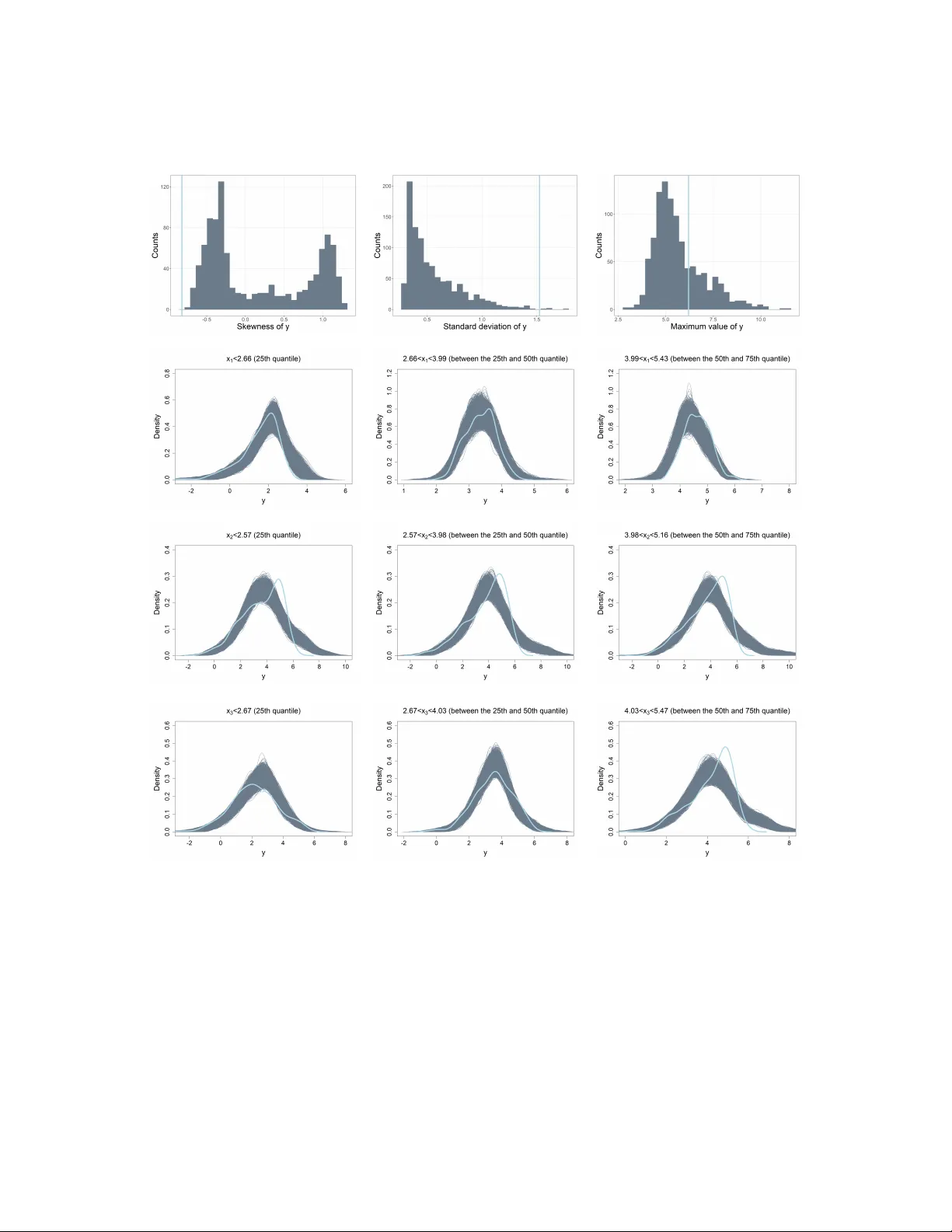
The generalized underlap co eﬃcien t with an application in clustering Zhao xi Zhang 1 , V anda In´ acio 1 , Sara W ade 1 1 Sc ho ol of Mathematics, Universit y of Edinburgh, Scotland, UK Abstract Quan tifying distributional separation across groups is f undamen tal in statistical learning and scientiﬁc disco very , y et most classical discrepancy measures are tailored to tw o-group com- parisons. W e generalize the underlap coeﬃcient (UNL), a m ulti-group separation measure, to m ultiv ariate v ariables. W e establish k ey properties of the UNL and pro vide an explicit con- nection to total v ariation. W e further interpret the UNL as a dep endence measure b etw een a group lab el and v ariables of interest and compare it with mutual information. W e prop ose an eﬃcien t imp ortance sampling estimator of the UNL that can be combined with ﬂexible density estimators. The utility of the UNL for assessing partition-cov ariate dep endence in clustering is highlighted in detail, where it is particularly useful for ev aluating whether the laten t group structure can b e explained b y sp eciﬁc cov ariates. Finally we illustrate the application of the UNL in clustering using tw o real world datasets. Keywor ds: Underlap co eﬃcien t, clustering, importance sampling, distributional separation, depen- dence. 1. In tro duction Statistical analysis often requires quantifying the distributional discrepancy across groups. This is essential in many tasks, suc h as quan tifying diﬀerences across exp erimen tal conditions, ev aluating classiﬁcation p erformance, and v alidating if identiﬁed clusters are meaningful. In many settings, it is necessary to go b ey ond simple mean comparisons and account for heterogeneity in the entire shap e, spread, and tail b eha vior of the distributions. F or the t wo-group setting, a ric h literature provides probability metrics and divergences, including total v ariation distance, Hellinger distance, and Kullbac k-Leibler (KL) divergence (see, e.g., Gibbs and Su, 2002, for a review). Suc h measures are central in machine learning and statistics: for instance, v ariational inference minimizes a KL divergence to the p osterior (Jordan et al., 1999), and classical GANs optimize an ob jective closely related to Jensen-Shannon divergence (Goo dfellow et al., 2020). The o verlap co eﬃcien t (OVL), the common area under t wo univ ariate densities, is directly linked to total v ariation distance (Sc hmid and Schmidt, 2006). It was introduced in W eitzman (1970a) and has since b een used as a non-directional alternative to ROC-based summaries for biomarker accuracy (e.g., In´ acio and Garrido Guill´ en, 2022). The underlap co eﬃcient (UNL) w as recently prop osed as a multi-group 1 Zhaoxi Zhang, School of Mathematics, University of Edinburgh, Scotland, UK (Z.Zhang-156@sms.ed.ac.uk). V anda In´ acio, Sc ho ol of Mathematics, Universit y of Edinburgh, Scotland, UK (V anda.Inacio@ed.ac.uk). Sara W ade, School of Mathematics, Universit y of Edinburgh, Scotland, UK (sara.wade@ed.ac.uk). 1 generalization of OVL and studied as a summary measure of univ ariate biomarker discriminatory ability (Zhang et al., 2025). In this article, we generalize the original deﬁnition of the UNL to multiv ariate v ariable spaces, th us pro viding a multi-group separation measure that can handle con tinuous, discrete, and mixed con tinu- ous–discrete v ariables. W e establish a uniﬁed measure-theoretic formulation and inv estigate the general prop erties of the UNL, b eyond its previously studied connections to ROC-based measures in the univ ariate case (Zhang et al., 2025). It is worth noting that the deﬁnition of the UNL for contin uous v ariables coin- cides with the deﬁnition of the “generalized L 1 -distance” b etw een K densities prop osed in Pham-Gia et al. (2008). W e further interpret UNL more broadly as an index of statistical dependence b etw een the group lab el and v ariables of interest, and compare it with the m utual information (MI) which has b een used across man y scientiﬁc domains as a general-purp ose dep endence measure. Additionally , w e develop an imp or- tance sampling algorithm to estimate the UNL. While Zhang et al. (2025) provides a grid-based numerical in tegration approach for estimating the UNL in the univ ariate case, such approaches b ecome computation- ally prohibitive in higher dimensions. The prop osed imp ortance sampling estimator provides a scalable alternativ e and can b e paired with Bay esian or frequentist density estimation pro cedures. W e demonstrate the utility of UNL in assessing partition-co v ariate dep endence in cluster analysis. In man y applications, the group structure is not observed and a common strategy is to discov er latent homogeneous groups within a heterogeneous p opulation via clustering. Once a partition has b een obtained, an imp ortant question is whether the inferred cluster lab els can b e explained by additional cov ariates (e.g., genot yp es, so cioeconomic status, or environmen tal factors). The UNL provides a direct wa y to quantify this dep endence by measuring the separation of cov ariate distributions across clusters. Adv ances in clustering allow co v ariate information to b e incorp orated, through formulations such as the mixture of exp erts (MOE, Mu and Lin, 2025). When constructing the MOE arc hitecture, a popular simpliﬁcation assumes single weights , under which cluster w eights do not v ary with cov ariates, implying that the inferred partition is indep enden t of cov ariates. Violating this assumption can lead to extremely p oor predictive inference in certain cases (W ade and In´ acio, 2025). In such cases, the UNL provides a v aluable complemen t to posterior predictive c hecks, oﬀering a scalar diagnostic that can ﬂag po or predictiv e p erformance of single-weigh t mixture mo dels, and provide insight into where mo del adjustments may b e needed, particularly whether or not to allow weigh ts to dep end on sp eciﬁc cov ariates. The rest of this paper is organized as follo ws. In Section 2, w e in troduce the generalized UNL, in vestigate its properties, connect it with the total v ariation, provide a comparison with mutual information, and present an estimation algorithm of UNL based on imp ortance sampling. In Section 3, we illustrate how to use the UNL to ev aluate the dep endence of a partition on cov ariates in cluster analysis. In Section 4, we illustrate the application of UNL in clustering using (i) a breast cancer genomic dataset and (ii) a dataset examining the inﬂuence of the p esticide DDT on the gestational age at delivery . 2. The generalized underlap co eﬃcient The UNL was introduced in Zhang et al. (2025) as a summary measure of the discriminatory abilit y of con tinuous univ ariate biomarkers. Beyond classiﬁcation problems, UNL can b e viewed more generally as a separation metric for arbitrary collections of distributions. In particular, its geometric formulation makes the concept natural in higher-dimensional v ariable spaces for v ariables that may be contin uous, discrete, or a mixture of b oth, as deﬁned formally in Deﬁnitions 1-4. Deﬁnition 1 (UNL for contin uous v ariables) . F or K gr oups, let X 1 , . . . , X K ∈ R p have prob ability densities f 1 , . . . , f K . The (c ontinuous) underlap c o eﬃcient is UNL( f 1 , . . . , f K ) = Z R p max 1 ≤ k ≤ K f k ( x ) dx. 2 Deﬁnition 2 (UNL for discrete v ariables) . F or e ach gr oup k = 1 , . . . , K , let X k = ( X k 1 , . . . , X kp ) take values in the ﬁnite or c ountably inﬁnite pr o duct spac e S = S 1 × · · · × S p , wher e S j is the state sp ac e of the j th c ate goric al variable. Deﬁne the gr oup-sp e ciﬁc pr ob ability mass function: p k ( x 1 , . . . , x p ) = Pr { X k 1 = x 1 , . . . , X kp = x p } , ( x 1 , . . . , x p ) ∈ S. The (discr ete) underlap c o eﬃcient is UNL( p 1 , . . . , p K ) = X ( x 1 ,...,x p ) ∈S max 1 ≤ k ≤ K p k ( x 1 , . . . , x p ) . Deﬁnition 3 (UNL for mixed type v ariables) . F or e ach gr oup k = 1 , . . . , K , X k = ( X c k , X d k ) with X c k ∈ R p and X d k ∈ S , let the joint pr ob ability density function b e f k ( x c , x d ) = f c k ( x c | x d ) p d k ( x d ) . The (mixe d) underlap c o eﬃcient is UNL( f 1 , . . . , f K ) = X x d ∈ S Z R p max 1 ≤ k ≤ K f k ( x c , x d ) dx c . Deﬁnition 4 (Measure theoretic formulation of UNL) . Let ( X , B , ν ) b e a σ –ﬁnite me asur e sp ac e and let P 1 , . . . , P K b e pr ob ability me asur es absolutely c ontinuous with r esp e ct to ν , with R adon-Niko dym derivatives f k ( x ) = dP k /dν ( x ) . The (gener al) underlap c o eﬃcient is UNL( f 1 , . . . , f K | ν ) = Z X max 1 ≤ k ≤ K f k ( x ) dν ( x ) . Cho osing ν as (i) the L eb esgue me asur e, (ii) a counting me asur e, or (iii) the pr o duct of the L eb esgue me asur e and a c ounting me asur e r e c overs Deﬁnitions 1–3, r esp e ctively. The UNL is bounded b et ween one and the n umber of groups K and can be interpreted as the “eﬀective” n umber of distinguishable distributions among the K groups. A v alue of K indicates complete separation of X across groups, signifying the presence of K distinct “eﬀective” distributions without any ov erlap across groups. Conv ersely , a v alue of one suggests that only one “eﬀective” distribution exists, as all K groups share one common distribution together. In termediate v alues betw een one and K corresp ond to partial separation, with higher v alues indicating a greater degree of separation. 2.1 Prop erties of the underlap co eﬃcien t Prop ert y 1 (Marginal monotonicity of UNL for contin uous v ariables) . L et I ⊆ { 1 , 2 , . . . , p } index a subset of variables and I c denote its c omplement. F or e ach class k = 1 , · · · , K , X k = ( X kI , X kI c ) is p artitione d into two sets, taking values in R | I | and R p −| I | , resp e ctively. Deﬁne the mar ginal pr ob ability density function of X kI as: g k ( x I ) = Z R p −| I | f k ( x ) dx I c , k = 1 , · · · , K. The UNL has the pr op erty: UNL( f 1 , . . . , f K ) ≥ UNL( g 1 , . . . , g K ) . The pro of of Prop ert y 1 is provided in the App endices, along with the pro ofs of all other prop erties and prop ositions. Analogous results of the UNL for discrete and mixed type v ariables are also established there. This marginal monotonicity of the UNL conﬁrms that it b eha ves in an intuitiv e wa y as a measure of sepa- ration across groups: including additional v ariables can only main tain or increase the degree of separation across groups and can never reduce it. Moreov er, the prop ert y shows that, when the UNL is interpreted more broadly as an index of statistical dependence b et ween the group lab el and the explanatory v ariable, it is information monotone: augmen ting the v ariable set cannot decrease the measured dep endence. In high–dimensional settings, where the UNL of the full joint density is diﬃcult to estimate precisely , the 3 v alue computed on a low er–dimensional subset of v ariables therefore provides a conserv ative yet informa- tiv e low er b ound b enc hmark. Moreo ver, the diﬀerence UNL( f 1 , . . . , f K ) − UNL( g 1 , . . . , g K ) quantiﬁes the marginal contribution of the omitted v ariables and can serve as a ranking criterion for v ariable selection pro cedures. Prop ert y 2 (T ransformation in v ariance of UNL for contin uous v ariables) . L et X 1 , . . . , X k ∈ R p have pr ob ability density functions f 1 , . . . , f k . Consider a c ontinuously diﬀer entiable, invertible map ψ : R p → R p with everywher e–p ositive Jac obian determinant | J ψ ( x ) | > 0 . The UNL satisﬁes UNL ( f 1 , . . . , f k ) = UNL ( f ψ 1 , . . . , f ψ k ) , wher e f ψ i ( u ) = f i  ψ − 1 ( u )  / | J ψ − 1 ( u ) | is the density of U i = ψ ( X i ) . This prop erty extends the univ ariate result of Zhang et al. (2025) to multiv ariate settings with an arbitrary ﬁnite n umber of groups and applies generally to discrete, contin uous, and mixed type v ariables. It should b e noted that transforming contin uous resp onse may hav e an adv antage in mo deling the densities in some cases, but transforming discrete resp onses usually do es not hav e the same adv antages for mo deling purp oses. Also, the inv ariance prop ert y is usually not preserved by the estimators we prop ose. If the transformation is not in vertible, for example, when performing dimension reduction on con tin uous v ariables (e.g., PCA), the UNL is monotone: pro jecting on to a lo wer-dimensional subspace can only decrease (or leav e unchanged) UNL. This supp orts the common b elief that dimension reduction typically entails information loss. Prop ert y 3 (Monotonicity of UNL for contin uous v ariables under linear dimension reduction) . L et A ∈ R q × p have ful l r ow r ank q ≤ p . F or e ach k = 1 , . . . , K , let f k b e the pr ob ability density of X k on R p , and let g k b e the pr ob ability density of AX k on R q . Then UNL( f 1 , . . . , f K ) ≥ UNL( g 1 , . . . , g K ) . The widely accepted manifold hypothesis p osits that many high-dimensional datasets lie on a low- dimensional manifold embedded in a high-dimensional space (Cayton, 2005). This has motiv ated a broad range of dimension-reduction methods. In practice, ho wev er, the choice of metho ds (and the target di- mensions) is often sub jective and dep ends strongly on the scientiﬁc ob jectiv e. F or group structured data, man y commonly used dimension-reduction techniques are unsup ervised and therefore do not explicitly in- corp orate group lab el information. If the primary goal is to preserve group separation as muc h as p ossible in the reduced represen tation, the UNL oﬀers a natural criterion: it can b e used to guide the choice of the num b er of reduced dimensions and to compare comp eting dimension reduction metho ds by assessing ho w well the resulting embedding retains distributional separability across groups (see e.g., the comparison b et ween PCA and PCA+t-SNE in the adult planarian cell genomic example in Whiteley et al. (2022)). 2.2 Connecting the underlap co eﬃcien t with total v ariation The total v ariation distance is a canonical metric quan tifying the discrepancy betw een t wo probability measures. Man y other statistical distances and divergence metrics (such as Hellinger distance and v arious f-div ergences) admit comparison inequalities with total v ariation or can b e controlled in terms of it (Gibbs and Su, 2002). F or t wo probabilit y measures P 1 and P 2 on ( X , B ), the total v ariation distance is TV( P 1 , P 2 ) = sup A ∈B   P 1 ( A ) − P 2 ( A )   , and can b e in terpreted as the largest possible diﬀerence in probabilities that the tw o measures assign to the same measurable even t. Prop osition 1 (UNL’s relationship with total v ariation distance when K = 2) . Supp ose P 1 and P 2 ar e pr ob ability measur es absolutely c ontinuous with r esp e ct to ν , with R adon-Niko dym derivatives f 1 and f 2 , then UNL ( f 1 , f 2 ) = 1 + TV ( P 1 , P 2 ) 4 More generally , deﬁne a vector-v alued measure µ as a vector consisting K probabilit y measures: µ : B − → R K , µ ( A ) =  P 1 ( A ) , . . . , P K ( A )  . The corresponding total v ariation norm of µ is: ∥ µ ∥ TV = sup π P A ∈ π ∥ µ ( A ) ∥ , where the supremum is tak en o ver all ﬁnite measurable partitions π of X . This con- struction extends the concept of total v ariation distance b et ween t wo probability measures to total v ari- ation norm of a sp eciﬁc sp eciﬁcation of a vector measure (Dinculeanu, 2014). If adopting the ℓ ∞ norm ∥ x ∥ ∞ = max 1 ≤ k ≤ K | x k | , the total v ariation norm is then: ∥ µ ∥ TV , ∞ = sup π X A ∈ π ∥ µ ( A ) ∥ ∞ = sup π X A ∈ π max 1 ≤ k ≤ K P k ( A ) . Prop osition 2 (UNL equals total v ariation norm of a vector-v alued measure consisted of K probability measures) . The underlap of the densities f 1 , . . . , f K satisﬁes UNL( f 1 , . . . , f K ) = Z X max 1 ≤ k ≤ K f k ( x ) dν ( x ) = ∥ µ ∥ TV , ∞ . 2.3 Comparing the underlap co eﬃcien t with mutual information Mutual information (MI) is a classical information–theoretic measure of statistical dependence b et ween t wo random v ariables whic h quantiﬁes how muc h uncertain ty ab out one v ariable is reduced by observing the other. It has b een applied across many scientiﬁc domains as a general-purp ose dep endence measure, and is extensively used as criteria in a large family of feature selection methods (see e.g. V ergara and Est ´ evez, 2014). In this subsection, we compare the UNL with MI as measures of dep endence b et ween a categorical v ariable Z , enco ding group lab els, and a (p ossibly high–dimensional) v ariable X . W e highlight the diﬀerences b et ween the tw o measures and discuss their practical implications. F or simplicity , we carry out the comparison under the assumption that X is contin uous (i.e. X ∈ R p ). Let Z take v alues in { 1 , . . . , K } , and supp ose ( Z, X ) has joint density p Z,X ( k , x ) = π k f k ( x ), where π k = P( Z = k ) and f k is the conditional density of X giv en Z = k . The mutual information I ( Z ; X ) is the Kullbac k–Leibler divergence b et ween the joint law and the pro duct of its marginals: I ( Z ; X ) = K X k =1 Z R p p Z,X ( k , x ) log p Z,X ( k , x ) π k p X ( x ) dx, p X ( x ) = K X k =1 π k f k ( x ) . Equiv alen tly , I ( Z ; X ) = E ( Z,X ) h log p Z,X ( Z, X ) / ( p Z ( Z ) p X ( X )) i , measured in nats when the natural loga- rithm is used (or in bits when log 2 is used). It is common to normalize MI by an entrop y based factor so that the result lies in [0 , 1] (Vinh et al., 2010). Popular choices include MI min = I ( Z ; X ) min { H ( Z ) , h ( X ) } , MI max = I ( Z ; X ) max { H ( Z ) , h ( X ) } . where H ( · ) denotes the Shannon entrop y and h ( · ) denotes the diﬀerential entrop y . Mutual information quantiﬁes ho w far the join t distribution p Z,X deviates, on a verage, from the product of its marginals p Z p X . The quantit y I ( Z ; X ) can b e interpreted as the amount of information that Z and X share, accessible symmetrically from Z to X and from X to Z , without privileging either direction. By con trast, UNL is inheren tly directional: it only captures the dep endence of Z on X through the degree of separation across the group-sp eciﬁc densities { f k ( x ) } K k =1 . The normalized quan tity MI Z = I ( Z ; X ) /H ( Z ) also quan tiﬁes the dep endence of Z on X , by measuring the proportion of uncertaint y in Z that is remov ed (or “explained”) by observing X . Nonetheless, MI Z and UNL target diﬀeren t asp ects of the dep endence: MI Z reﬂects information ﬂow, whereas UNL reﬂects geometric separability of the distributions across groups. W e compare UNL with MI Z in the following illustrativ e examples. 5 Illustrativ e examples comparing UNL with MI. Consider three groups with X | Z = k ∼ N( µ k , 1) , k ∈ { 1 , 2 , 3 } . W e start by ﬁxing µ 2 = 0 and set µ 1 = − D , µ 3 = D for D ∈ [0 , 6] and we also ﬁx µ 1 = − 0 . 1, µ 2 = 0, and v ary µ 3 = D for D ∈ [0 , 6]. This yields the curves of UNL versus MI Z in Figure 1, under (i) a balanced prev alence scenario Pr( Z = 1) = Pr( Z = 2) = Pr( Z = 3) = 1 / 3, and (ii) a highly imbalanced scenario Pr( Z = 1) = Pr( Z = 3) = 0 . 495 , Pr( Z = 2) = 0 . 01. F rom the top row of Figure 1 w e see that when the three groups are either identical or p erfectly separated, UNL and MI Z b eha ve in a qualitatively similar w ay , regardless of whether the group prev alences are balanced or imbalanced. When the three groups are identical, UNL = 1 and MI Z = 0, indicating no dep endence of Z on X . When the three groups are p erfectly separated, UNL = 3 and MI Z = 1, indicating that Z can be determined exactly from X . As D increases, MI Z and UNL follow a similar trend, although the relationship b et ween them is nonlinear. This nonlinearity b ecomes more pronounced as the group prev alences b ecome imbalanced. While UNL and MI ma y agree qualitativ ely when the groups are either perfectly separated or completely iden tical, the implication of their results are diﬀerent particularly in some settings with partial separation and imbalanced group prev alences. As shown in the b ottom row of Figure 1, when the class prev alences are extremely imbalanced, the increase in MI Z as µ 3 mo ves aw a y from µ 1 and µ 2 is almost negligible. In most empirical con texts, the v alues of MI Z w ould b e considered numerically small and diﬃcult to distinguish from noise. By contrast, UNL increases from approximately 1 . 04 to 2 . 04. This clearly illustrates the philosophical diﬀerence b et ween UNL and MI. MI is a prev alence–av eraged metric: eac h group contributes to I ( Z ; X ) and hence to MI Z in prop ortion to its prev alence. A p erfectly separable but rare group therefore contributes almost nothing to MI Z . In contrast, every group contributes equally to UNL, even for rare groups. MI (or MI Z ) captures how often the dep endence structure matters in the p opulation, while UNL targets if the dep endence structure is present at all. This prev alence–free prop ert y is particularly imp ortant in biomedical and ﬁnancial applications where rare but distinct groups (e.g., rare toxicit y phenot yp es, rare cell states, defaulters) are of primary scientiﬁc in terest. In such set- tings, MI underplays their imp ortance by av eraging ov er the p opulation, whereas UNL directly reﬂects the “eﬀectiv e” num b er of categories supp orted by the v ariables. 2.4 Estimation of UNL b y imp ortance sampling Estimating the UNL is essentially ev aluating the non–ov erlapping probability mass across the group–conditional distributions. W e prop ose a pro cedure based on imp ortance sampling to estimate UNL. W e fav our imp ortance sampling ov er other Monte Carlo approaches such as Marko v chain Monte Carlo (MCMC) b ecause the samples pro duced by an imp ortance sampling sc heme are indep enden t, in contrast to the serially correlated draws generated by MCMC. This indep endence makes the computation amenable to parallel implementation, thereby improving computational eﬃciency . The imp ortance sampling pro cedure for estimating UNL is outlined in Algorithm 1. W e describ e the setting in which the densities of each group are obtained in a Bay esian framework, but the same strategy can be applied with alternative density estimators: one should simply plug the corresponding estimated densities into the importance sampling sc heme. The accuracy and eﬃciency of importance sampling hinge on a wise choice of proposal densit y q ( x ). It is crucial that q ( x ) > 0 wherever max 1 ≤ k ≤ K f k ( x ) is nonzero to ensure that the ratio max 1 ≤ k ≤ K f k ( x ) /q ( x ) is w ell-deﬁned. Ideally , q ( x ) should b e chosen such that the v ariance of the estimator is minimized. Here, we set the prop osal distribution as the mixture of the K group densities: q ( x ) = P K k =1 π k f k ( x ). A conv enient c hoice is the equally weigh ted mixture q ( x ) = 1 /K P K k =1 f k ( x ) , obtained by setting π k = 1 /K . This equally-w eighted mixture prop osal has tw o attractive prop erties: (i) supp orted match: because q ( x ) is p ositive wherev er any f k ( x ) is p ositiv e, hence the imp ortance ratio is well deﬁned on the entire 6 Figure 1: Curv es of UNL and MI Z in the three-class Gaussian example, where Y | Z = k ∼ N( µ k , 1) and µ 1 = − D , µ 2 = 0 , µ 3 = D (top row), and where where Y | Z = k ∼ N( µ k , 1) and µ 1 = − 0 . 1 , µ 2 = 0 , µ 3 = D (b ottom row). supp ort of the en velope; (ii) b ounded weigh ts: for every x i , 1 ≤ max 1 ≤ k ≤ K f k ( x i ) q ( x i ) = max 1 ≤ k ≤ K f k ( x i ) 1 K P K k =1 f k ( x i ) ≤ K, so the weigh ts can never explo de, this yields the v ariance b ound: V ar  [ UNL  ≤ UNL( K − UNL) / M . The deriv ation of the exact v ariance of the imp ortance sampling estimator of UNL, together with an upp er b ound, is given in the App endices. The b ound implies that when UNL = K (i.e., the K groups are perfectly separated), V ar  [ UNL  = 0. When UNL = 1 (i.e., all groups are identical), the bound gives V ar  [ UNL  ≤ ( K − 1) / M . In both extremes the v ariance b ound is small. Moreo ver, when UNL = 1, the equal-weigh t mixture prop osal 1 /K P K k =1 f k ( x ) coincides with max 1 ≤ k ≤ K f k ( x ), so the importance sampling weigh ts are constant and the estimator v ariance is in fact zero, the b ound is therefore conserv ative in this regime. Deriving tighter v ariance b ounds that better capture suc h cases is an interesting direction for future work. Nev ertheless, even this coarse b ound can guide the choice of the Mon te Carlo sample size M . F or example, if σ 2 0 denotes a maximum acceptable v ariance, a conserv ative c hoice is M = K 2 /σ 2 0 whic h ensures V ar  [ UNL  ≤ σ 2 0 under the b ound. A visual illustration of the v ariance b ound for K = 5 is provided in the App endices. It is worth noting that Algorithm 1, combined with the equal-weigh t mixture prop osal, is exactly the R 2 m ultiple imp ortance sampling scheme describ ed in Elvira et al. (2019). 7 Algorithm 1 Imp ortance sampling pro cedure for estimating UNL for contin uous v ariables Step 1: Densit y estimation: Estimate the density of X for every group, i.e., estimate f k ( x ), for k ∈ { 1 , · · · , K } . In the Bay esian con text, p osterior realizations of the density estimate for group k would b e denoted as f ( s ) k ( x ) for s = 1 , 2 , · · · , S , where S represen ts the n umber of samples (e.g., iterations of the MCMC sampler after burn-in, dra ws in predictiv e mo delling (F ong et al., 2023)). for s = 1 , 2 , . . . , S do Step 2: Dra w samples from the prop osal distribution q ( s ) ( x ) : Generate M iid samples x i from q ( s ) ( x ). for i = 1 , 2 , . . . , M do Compute the imp ortance weigh ts: w ( s ) i = max 1 ≤ k ≤ K f ( s ) k ( x i ) /q ( s ) ( x i ) . end for Step 3: Calculate the sample av erage of weigh ts: Compute the imp ortance sampling estimate of the UNL: [ UNL ( s ) = 1 M M X i =1 w ( s ) i . end for In terv als of { [ UNL ( s ) } S s =1 reﬂect uncertaint y arising from mo delling the densities given the observed data in each group. 3. UNL as a to ol for disco v ering cov ariate dep endence in cluster analysis Man y scien tiﬁc problems inv olve assessing ho w group structure relates to external v ariables. When group lab els are observed, the UNL provides a direct wa y to quantify the dep endence of these lab els on other v ariables by measuring the degree of separation across groups. In many applications, how ever, the group structure is unobserved, and a common strategy is to discov er latent group structure via clustering. A wide v ariety of clustering metho ds has b een prop osed (see e.g., Saxena et al., 2017, for a review). In this pap er, we fo cus on mo del-based clustering, with particular emphasis on Ba yesian mixture mo dels, although the proposed approach applies more broadly . W e sho w how the UNL can be used to assess ho w an inferred partition relates to cov ariates. Dep ending on whether clustering is p erformed using only the resp onse (the marginal approach) or via a mixture mo del that explicitly incorp orates cov ariates (the conditional approach), the inferred partition may comprise clusters of individuals with similar resp onses or clusters of individuals with similar response–cov ariate relationships. 3.1 Clustering based only on the resp onse The marginal approac h of mixture mo dels. In mixture mo dels, the observed data are mo deled as rising from a mixture of simpler comp onent distributions, with each comp onen t corresponding to a cluster (F raley and Raftery, 2002). If co v ariate information is not considered, mixture mo dels assume the data y 1 , . . . , y n (here we use y to denote the data vector b eing clustered, to distinguish from cov ariates x introduced later) are conditionally i.i.d. from a conv ex combination of parametric comp onents (W ade, 2023): y i iid ∼ L X l =1 w l K ( · | θ l ) = Z K ( · | θ ) dH ( θ ) , (1) 8 where K ( y | θ ) is a ﬁxed parametric density , often referred to as the kernel, with comp onent-speciﬁc parameters contained in θ = ( θ 1 , . . . , θ L ). In the equiv alent integral represen tation on the right-hand side of (1), H = P L l =1 w l δ θ l represen ts the mixing measure with the mixture weigh ts w = ( w 1 , . . . , w L ) that are non-negative and sum to one. Y et another equiv alent representation, useful for clustering, makes use of allo cation v ariables z = ( z 1 , . . . z n ): y i | z i = l, θ l iid ∼ f ( · | θ l ) , z i iid ∼ Cat( w 1 , . . . , w L ) , where Cat( · ) represents the categorical distribution with parameter w . In the Bay esian setting, the mo del in (1) is completed with a prior on the unknown parameters w and θ (or equiv alen tly on the unknown mixing measure H ). Additionally , Bay esian nonparametric mo dels allo w the num b er of clusters to b e not ﬁxed in adv ance, by assuming an inﬁnite num b er of comp onen ts and can b e viewed as a limiting case of ov erﬁtted mixtures, with the Dirichlet pro cess mixture (DPM) b eing the most-widely used example (W ade, 2023). The DPM mo del uses a Dirichlet pro cess (DP) prior (F erguson, 1973) on the mixing measure ( H ∼ DP( α, H 0 )). According to Sethuraman’s stic k-breaking representation (Seth uraman, 1994), H can b e expressed as: H = ∞ X l =1 w l δ θ l (2) where w 1 = v 1 , w l = v l Q l − 1 m =1 (1 − v m ), for l ≥ 2, with v l iid ∼ Beta(1 , α ), for l ≥ 1. Under (2), the probabilities assigned to each comp onent decrease rapidly with the index l for typical c hoices of α . Consequen tly , the inﬁnite mixture mo del can b e reasonably approximated by a ﬁnite n umber of components. F or this reason, p osterior inference can b e conducted using the blo c ked Gibbs sampler (Ish waran and James, 2001), which truncates Sethuraman’s representation in (2) to a ﬁnite v alue, L , with v L = 1 to ensure that the mixture w eights sum to one. F or example, the model structure and prior sp eciﬁcation of a DPM mixture mo del with kernel as the pro duct of multiv ariate normal and categorical distributions which is implemen ted in this pap er are provided in the App endices. Detecting dep endence of the partition on co v ariates in the marginal approach. In the marginal approac h, clustering is performed solely on the response, thereby assigning observ ations with simi- lar outcomes to the same cluster. T o assess whether, and to what extent, cov ariates inﬂuence the clustering partition structure, w e propose to use the UNL of cov ariates, as deﬁned in Deﬁnitions 1–4, to quantify partition–co v ariate dep endence by measuring the separation of co v ariate distributions across clusters. Low underlap v alues indicate substantial ov erlap in cov ariate distributions across clusters, suggesting weak de- p endence of the inferred partition on the cov ariates, whereas high underlap v alues reﬂect more distinct co v ariate distributions and hence stronger dep endence of the partition structure on cov ariates. While it is diﬃcult to visually assess cov ariate diﬀerences across clusters when the cov ariates are multiv ariate, the UNL provides a concise quantitativ e summary of ho w strongly a resp onse-based partition dep ends on the co v ariates. In a Bay esian setting, estimating the UNL for every p osterior draw of the partition requires (i) estimating the density of co v ariates for each cluster in each sampled partition and (ii) calculating the UNL for ev ery p osterior dra w of the density estimates for every partition, which is computationally exp ensiv e. W e instead prop ose to estimate UNL for a single represen tative partition, speciﬁcally , the point estimate that minimizes the Jensen’s-inequalit y low er b ound to the posterior exp ected V ariation of Information (VI W ade and Ghahramani, 2018). This choice has the desirable prop erties of VI as a metric on partitions with an information-theoretic in terpretation (Meil˘ a, 2007), while remaining computationally tractable b ecause the b ound depends only on the p osterior similarit y matrix. Other choices of the representativ e partition, based on alternative loss functions, could also b e considered, but we adopt the VI-based estimator for its b eneﬁts highligh ted in W ade and Ghahramani (2018). T o accoun t for uncertain ty while also retaining computational 9 eﬃciency , a simple approach is to summarize the p osterior with multiple represen tative partitions produced b y the W ASABI metho d (Balo cchi and W ade, 2025, see the App endices for details). W e illustrate the utilit y of the UNL in quan tifying partition-co v ariate dependence through tw o sim ulated examples, which represen ts distinct data-generating mechanisms with diﬀerent relationships b etw een the resp onse y and cov ariates x . In b oth, the DPM is used for clustering and for estimating the cov ariate densities within each group, giv en the representativ e partition. The DPM is ﬁt using the sp eciﬁcations detailed in the App endices. P osterior inference is based on 10,000 MCMC iterations after discarding an initial burn-in of 10,000 iterations. Given the density estimates, the UNL is computed via imp ortance sampling (Algorithm 1) using a Monte Carlo sample size of M = 5000, which yields v ariance upp er b ounds of 9 / 5000 and 4 / 5000 for the tw o examples, resp ectiv ely . Example A (cluster assignmen ts fully determined b y a single co v ariate). W e generate n = 600 observ ations according to y i = 2 1 ( x i ≤ − 1) − 5 1 ( x i ≥ 1) + ϵ i , ϵ i ∼ N(0 , 0 . 1 2 ), with x i ∼ Unif ( − 3 , 3). Example B (cluster assignmen ts dep end join tly on t wo cov ariates but not on either marginally). W e generate n = 600 observ ations from y i = m ( x i ) + ϵ i , ϵ i ∼ N(0 , 0 . 1 2 ), where x i = ( x i 1 , x i 2 ) T , x ij ∼ Unif ( − 2 , 2), and m ( x i ) = 1 (sin( x i 1 x i 2 π / 2) ≤ 0) − 1 (sin( x i 1 x i 2 π / 2) > 0). The representativ e partition structures obtained from the mixture mo del, together with the histograms of the estimated UNLs for Examples A and B, are shown in Figure 2. In Example A, the cov ariate x is almost p erfectly separated across clusters, and consequently the UNL is very close to the num b er of inferred clusters ( K = 3). Example B, which is also considered in W ade and In´ acio (2025), exhibits a diﬀeren t pattern: the estimated UNL for the joint distribution of ( x 1 , x 2 ) is again close to the num b er of inferred clusters ( K = 2), indicating pronounced dep endence of the inferred partition on ( x 1 , x 2 ) jointly . By contrast, the UNL v alues for the marginal distributions of x 1 and x 2 are each near one, indicating little partition–cov ariate dep endence when each cov ariate is considered marginally . This pattern illustrates a signiﬁcant join t cov ariate eﬀect without any signiﬁcant marginal eﬀect: neither co v ariate alone explains the partition, but their joint conﬁguration do es. It is also worth noting that, once the join t density has b een estimated using a DPM of multiv ariate normals, the marginal densities are a v ailable analytically by restricting the ﬁtted comp onen t parameters to the relev ant coordinates. Consequently , the UNL of the marginals can b e computed without reﬁtting the DPM mo del separately for eac h cov ariate. It is important to note that UNL quan tiﬁes the dep endence of a giv en partition on the co v ariates, rather than the dependence of the response on the cov ariates. Diﬀerent partition structures will, in general, induce diﬀeren t partition–cov ariate relationships. 3.2 Incorp orating co v ariate information in clustering The conditional approach of mixture mo dels. Unlike in the marginal approach, the conditional approac h of the mixture mo del explicitly mo dels the cov ariate-sp eciﬁc density f ( y i | x i ), allowing the distri- bution of y i to dep end on x i through cov ariate-dep enden t mixture weigh ts, cov ariate-dep enden t comp onen t parameters, or b oth. The general form of the conditional approac h assumes that the data y i arise from a combination of co v ariate-sp eciﬁc parametric comp onen ts for i ∈ { 1 , · · · , n } : y i | x i ∼ L X l =1 w l ( x i ) K ( · | θ l ( x i )) = Z K ( ·| θ ) dH x i ( θ ) , (3) where K ( y | θ ( x )) is a ﬁxed parametric density , with comp onen t-sp eciﬁc parameters contained in θ ( x ) = ( θ 1 ( x ) , . . . , θ L ( x )) and the mixture weigh ts w ( x ) = ( w 1 ( x ) , . . . , w L ( x )) are non-negative and sum to one for every p ossible x v alue. The eq uiv alent representation which mak es use of latent group v ariables z = ( z 1 , . . . z n ) is: y i | x i , z i = l ind ∼ f ( · | θ l ( x i )) , z i ind ∼ Cat( w 1 ( x i ) , . . . , w L ( x i ) , 10 Figure 2: T op ro w: Example A. Bottom ro w: Example B. Left: the represen tative partition inferred from the DPM. Right: histograms of the estimated UNL of the co v ariates. Similar to the marginal approach, priors on θ ( x ) and w ( x ) (or equiv alently on H x ) are required for Ba yesian inference of the mo delling. The dep enden t DP (DDP) (MacEachern, 1999) is a p opular nonpara- metric prior for the random probability mixing measures H x , whic h mo diﬁes the stick-breaking represen- tation of the DP to accommodate cov ariates and in full generality , and is sp eciﬁed as: H x = ∞ X l =1 w l ( x ) δ θ l ( x ) (4) where w 1 ( x ) = v 1 ( x ), w l ( x ) = v l ( x ) Q l − 1 m =1 (1 − v m ( x )), for l ≥ 2. v l ( x ) are indep enden t sto c hastic pro cesses with marginals following Beta(1 , α ( x )), and θ l ( x ) are also indep enden t stochastic pro cesses, for l ≥ 1. Similarly to the DPM mo del, the num b er of comp onen ts in (4) could b e truncated to a ﬁnite v alue, L , with v L ( x ) = 1, to facilitate p osterior inference. A frequen tly used class of DDPs is the single-w eights DDP , motiv ated primarily b y computational con venience: it reuses existing p osterior sampling algorithms for DPMs by restricting the mixing weigh ts to b e co v ariate-inv ariant, i.e., w l ( x ) ≡ w l . F or example, a p opular single-w eights DDP mo del which is often referred to as the linear dependent Diric hlet pro cess (LDDP) mixture model (see e.g., Quin tana et al., 2022; W ade and In´ acio, 2025) for modelling a con tinuous resp onse takes the form: f ( y i | x i ) = ∞ X l =1 w l ϕ ( y i | β T l x i , σ 2 l ) . (5) 11 where ϕ ( · ) represent the normal densit y function, and β T l x i and σ 2 l denote the mean function and the v ariance of comp onen t l respectively . Although the mo del may app ear highly ﬂexible and is computationally attractiv e, the induced predictive mean and conditional density are in fact quite constrained. The single- w eight LDDP mixture of normals yields a w eighted combination of linear regression functions but lacks the lo cal adaptation aﬀorded by cov ariate-dep enden t w eights. As a result, it ma y b e insuﬃcien tly ﬂexible for capturing complex regression relationships (W ade and In´ acio, 2025). The speciﬁc mo del structure and prior sp eciﬁcation for the LDDP mixture mo del implemented in this pap er are detailed in the App endices. Detecting dep endence of the partition on cov ariates in the conditional approach. In the conditional approac h, the mixture model groups individuals with similar resp onse-co v ariate relationship. Similar to the unconditional approach, we prop ose to use the UNL of cov ariates to assess the inﬂuence of co v ariates on the inferred clustering partition. This is particularly imp ortan t for the single-w eights mixture mo del, which p osits that the inferred partition has no dependence on co v ariates, assuming that the UNL of the co v ariates should b e one. Ho wev er, when the regression kernel is not suﬃciently ﬂexible, the inferred partition structure may dep end on the co v ariates. In suc h cases, the cluster-speciﬁc predictions are a veraged regardless of co v ariate v alues, b ecause the mixing weigh ts do not account for the similarity b et ween the new cov ariates x n +1 and the cov ariates within each cluster (W ade and In´ acio, 2025). As a consequence, predictive inference for the regression function, density , and associated uncertaint y under the single-w eights mixture can b e extremely p oor. W e consider three examples to illustrate the utility of the UNL in quantifying the partition-cov ariate dep endence in the conditional approach of mixture model. Examples C1 and C2 inv olve low-dimensional co v ariates, where dep endence of the LDDP-induced partition on co v ariates can b e visualized directly . Ex- ample D, in contrast, inv olves a higher-dimensional cov ariate space, where the dep endence pattern of the partition on all cov ariates is diﬃcult to observe visually , and here the UNL provides a systematic wa y to screen for and summarize partition–cov ariate dependence across man y cov ariates. Example C1 (lo w-dimensional cov ariate space with distinct slop es of x c across categories of x d ). W e generate n = 800 observ ations according to y i | x c i , x d i ∼    0 . 5N( − 2 x c i , 0 . 4 2 ) + 0 . 5N(2 x c i , 0 . 4 2 ) , if x d i = 1 , 0 . 5N( − 12 x c i + 80 , 0 . 4 2 ) + 0 . 5N(12 x c i + 80 , 0 . 4 2 ) , if x d i = 2 , where x c i ∼ Unif ( − 3 , 3) and Pr( x d i = 1) = Pr( x d i = 2) = 0 . 5. Example C2 (low-dimensional cov ariate space with common slop es of x c across categories of x d ). W e again generate n = 800 observ ations, now from y i | x c i , x d i ∼    0 . 5N( − 12 x c i , 0 . 4 2 ) + 0 . 5N(12 x c i , 0 . 4 2 ) , if x d i = 1 , 0 . 5N( − 12 x c i + 80 , 0 . 4 2 ) + 0 . 5N(12 x c i + 80 , 0 . 4 2 ) , if x d i = 2 , with x c i ∼ Unif ( − 3 , 3) and Pr( x d i = 1) = Pr( x d i = 2) = 0 . 5. The only diﬀerence b etw een Examples C1 and C2 in the data generating mechanism is the slop e of the x c when x d = 1, all other asp ects are iden tical. This seemingly minor change leads to markedly diﬀerent b eha vior under the LDDP mixture mo del: the representativ e partition inferred b y LDDP con tains four clusters in C1 but only tw o in C2 (see the left panel of Figure 3). In Example C1, clusters 3 and 4 consist exclusively of units with x d = 1, whereas clusters 1 and 2 consist exclusively of units with x d = 2. In Example C2, b y con trast, x d app ears more ev enly represen ted across the tw o clusters. This visible partition–co v ariate dependence in Example C1, and its absence in Example C2, is conﬁrmed b y the UNL v alues shown in the right panel of Figures 3. In Example C1, the estimated UNL v alues for b oth the marginal distribution of x d and the joint distribution ( x c , x d ) are large, indicating substantial dependence of the inferred partition on x d and thereb y 12 Figure 3: T op row: Example C1. Bottom row: Example C2. Left: the representativ e partition inferred from the DPM. Right: the histograms of the estimated UNL of the cov ariates. violating the single-weigh t assumption of the LDDP mixture mo del. By contrast, in Example C2 the UNL v alues are all close to one, indicating little partition–cov ariate dep endence. The diﬀerence in UNL v alues b etw een the tw o examples has clear predictive implications. In the LDDP mixture mo del, predictions are a veraged with mixing w eights that do not v ary with the cov ariates. In Example C1, the LDDP-induced partition exhibits mo derate dep endence on x d ; with cov ariate-constant w eights, this leads to p oor predictiv e p erformance. In Example C2, the partition shows little dep endence on either co v ariate, thus cov ariate-constant weigh ts do not degrade prediction. Heatmaps of the true and estimated density regression functions for Examples C1 and C2 conditional on x d = 1 are sho wn in Figure 4, the corresp onding plots for x d = 2 are provided in the Appendices. Example D (high-dimensional co v ariate space). W e generate 1000 observ ations following: y i | x i ind ∼ p ( x i 1 ) N ( y i | β 1 , 0 + β 1 , 1 x i 1 , σ 2 1 ) + (1 − p ( x i 1 )) N ( y i | β 2 , 0 + β 2 , 1 x i 1 , σ 2 2 ), where p ( x i, 1 ) = τ 1 exp ( − τ 2 1 2 ( x i, 1 − µ 1 ) 2 ) / [ τ 1 exp ( − τ 2 1 / 2( x i, 1 − µ 1 ) 2 ) + τ 2 exp ( − τ 2 2 / 2( x i, 1 − µ 2 ) 2 )] , with β 1 = (0 , 1) T , σ 2 1 = 1 / 16, β 2 = (4 . 5 , 0 . 1) T , σ 2 1 = 1 / 8, µ 1 = 4, µ 2 = 6, τ 1 = τ 2 = 2. Let p = 20 and x i = ( x i 1 , . . . , x ip ) ⊤ i.i.d. ∼ N p ( µ, Σ), with mean µ = (4 , . . . , 4) T and cov ariance matrix Σ sp eciﬁed as follo wing. Let Σ hh = 4 for all h and partition the co v ariate indices in to the o dd and even sets: O = { 1 , 3 , 5 , . . . , 19 } , E = { 2 , 4 , 6 , . . . , 20 } . Within-group cov ariates are correlated with correlation 0 . 75 while across-group cov ariates are indep endent. As sho wn in Figure 5, the LDDP mixture mo del identiﬁes tw o clusters in the represen tative partition. Although one can visually detect some dependence of the partition on x 1 , it is diﬃcult to assess ho w 13 Figure 4: Heatmap of the true and estimated density regression functions of Examples C1 and C2 conditioned on x d = 1. T op row: Example C1. Bottom row: Example C2. Figure 5: Left: the representativ e partition of Example D inferred from the LDDP mo del. Right: the histograms of the estimated UNL of the cov ariates of Example D. the clustering partition depends simultaneously on all cov ariates, or on the o dd/ev en-indexed subsets of co v ariates. Ho wev er, through the UNL v alues (Figure 5), we can detect that the LDDP-induced partition exhibits muc h stronger dep endence on the o dd-indexed co v ariates than on the even-indexed ones. This correctly reﬂects the data-generating mec hanism, in which only the odd-indexed cov ariates inﬂuence cluster 14 Figure 6: Example D: p osterior predictive chec ks for selected statistics (kurtosis and kernel densit y estimates), with the estimated statistics (light blue), sho wn alongside estimates from 5,000 datasets dra wn from the p osterior predictive distribution (grey). Figure 7: Example D: heatmap of the true density regression function and the estimated density regression function conditioned on x 2 to x 19 at the 25% quantiles. allo cation. Also, within the o dd group, the UNL for x 1 is only slightly smaller than the UNL for all o dd cov ariates jointly , indicating that most of the partition–cov ariate dep endence is driven by x 1 . This matc hes the construction of the example, where x 1 is the only cov ariate that informs the cluster allo cation probabilities. In this case, the po or predictive performance of the LDDP model, which ignores co v ariates in the mixing w eights, is therefore anticipated given the large UNL v alue. The discrepancy b et ween the true conditional densit y and the p osterior predictive conditional density is evident in Figure 15. Although several summary statistics of the posterior predictive distribution do not deviate severely from the observed v alues, the lack of ﬁt b ecomes clear in the kernel density estimates of the p osterior predictive distributions conditional on sev eral cov ariate in terv als, particularly for conditioning on x 1 or x 3 ab o ve their 75th p ercen tiles. Some selected p osterior predictive c hecks are presented in Figure 6 while the others are shown in the App endices. It might b e easy to ov erlo ok the lack of ﬁt if not c ho osing the correct p osterior chec k statistics, while the UNL can ﬂag this. This lack of ﬁt can b e easy to miss if statistics which illustrate the p o or predictive p erformance are not c heck ed, whereas UNL ﬂags the issue here. While p osterior predictive c hecks of conditional densities may reveal suc h mo del inadequacies, the UNL oﬀers insigh ts in to where to make mo del adjustments, particularly whether or not to allo w w eights to dep end on speciﬁc cov ariates. Moreov er, in real-world applications with high-dimensional cov ariates, kernel densit y estimates within conditioning interv als can b ecome unstable when the sample size is small. In these settings, UNL pro vides a v aluable complement to p osterior predictive chec ks, oﬀering a scalar diagnostic that can ﬂag p oor predictive p erformance of the single-weigh t mixture mo del when the partition dep ends strongly on cov ariates. 15 4. Real data illustrations This section illustrates the broad applicabilit y of the UNL for assessing partition-cov ariate dep endence in mo del-based clustering, through tw o real-data applications. In all cases, p osterior inference relies on 10000 iterations, after discarding the ﬁrst 10000 as a burn-in. T o ev aluate the underlap via imp ortance sampling (Algorithm 1), we use a Mon te Carlo sample size of M = 5000. 4.1 Breast cancer genomic analysis Breast cancer is a heterogeneous disease whose dev elopmen t and progression is complex and not fully under- sto od (Y ersal and Barutca, 2014). Characterizing this heterogeneity is essential for improv ed personalized treatmen t, and clustering metho ds provide a natural framework for uncov ering the latent structure. A substantial literature has inv estigated prognostic and therap eutic targets in breast cancer, numerous gene expression signatures were suggested as contributing to disease severit y and prognosis (e.g., Kallah- Dagadu et al., 2025; Shok o ohi et al., 2025). In this application, we focus on how the heterogeneit y structure in breast cancer prognosis can b e explained by the selected gene expression groups. As our clinical endpoint, w e c haracterize the prognosis b y the three clinicopathologic tumor characteristics which are used to calculate the Nottingham prognostic index (NPI) (Haybittle et al., 1982): histological grade (v arying from 1–3 with 3 as the most abnormal grade), lymph no de stage (v arying from 1–3 with 3 as the stage with the most p ositiv e lymph no des), and tumor size (mm). W e applied our methods to the MET ABRIC dataset, whic h pro vides clinical and genomic data on breast tumors from ﬁve diﬀerent hospitals/ research centers in the United Kingdom and Canada (Pereira et al., 2016). Guided by prior evidence on prognostic relev ance (Ay oub et al., 2024; T ang et al., 2015), w e fo cus on t wo gene groups: { MET, ESR1, ESR2 } and { BRCA1, BECN1 } . Of the 2509 patients in the dataset, 2040 had complete data on the tumor characteristics required for the NPI; among these, 1815 also had complete mRNA expression log intensit y v alues for the selected genes. Mo del-based clustering is p erformed on the 2040 cases with complete NPI tumor characteristics, whereas estimation of the UNL for the selected genes is restricted to the 1815 cases with complete gene-expression data. Although the NPI is widely used in clinical practice for prognostic stratiﬁcation following breast cancer surgery , it is a derived score. Clustering directly on the NPI may therefore reﬂect the near discrete nature of the score construction rather than its genuine latent structure (see the b ottom right panel in Figure 8). T o av oid this, we ﬁt a DPM mo del to the three tumor characteristics used to compute the NPI. It is an example of the marginal approach of mo del-based clustering as describ ed in Section 3. The kernel of DPM mo del takes the pro duct form: K ( y ; θ ) = N  y 1 ; µ, σ 2  Cat  y 2 ; p g1 , p g2 , p g3  Cat  y 3 ; p n1 , p n2 , p n3  , where y 1 , y 2 and y 3 represen t tumor size, histological grade and lymph no de stage, resp ectiv ely . As sho wn in Figure 8, cluster 1 exhibits the smallest tumor sizes, the low est prop ortion of the most abnormal histological grade (grade 3), and the low est prop ortion of adv anced lymph no de stage (stage 3); cluster 3 shows the opposite pattern. Therefore, cluster 1 corresp onds to the most fav orable prognosis and cluster 3 to the least fav orable. These ﬁndings suggest that patients in cluster 3 may w arrant consideration of more aggressive therapies. W e next quantify the dep endence of the clustering on the t wo gene groups, { MET, ESR1, ESR2 } and { BRCA1,BECN1 } , via the UNL. Figure 9 displays the histograms of the estimated UNL for each gene groups. The UNL of { MET, ESR1 } is larger than UNL of { MET, ESR2 } with high probabilit y (P(UNL MET&ESR1 > UNL MET&ESR2 ) = 0 . 99), suggesting that the co expression of MET and ESR1 is more informativ e for the clinicopathologic prognosis clusters than MET and ESR2. T ang et al. (2015) rep orted an asso ciation with prognosis for BECN1 but not BR CA1. Consistent with this, the estimated marginal underlap distribution for BECN1 is slightly shifted upw ard relative to that for BRCA1 (despite substantial o verlap in their histograms), with P(UNL BECN1 > UNL BRCA1 = 0 . 71). It should b e mentioned that, by themselv es, the mRNA expression of the selected genes only accounts for a small fraction of the three prognosis groups, incorp orating the expression of other gene groups and/or using multi-omics metho ds is 16 Figure 8: Cluster proﬁles of breast cancer prognostic factors, based on the single represen tative partition. Figure 9: Left panel: the histogram of estimated underlap for the { MET, ESR1, ESR2 } gene group based on the single representativ e partition. Right panel: the histogram of estimated underlap for the { BRCA1, BECN1 } gene group based on the single represen tative partition. suggested for further inv estigations. 17 4.2 Pregnancy term to xicology analysis Our second application, dra wn from epidemiology studies, has been used in numerous w orks for v ali- dating Bay esian nonparametric density regression mo dels (e.g., Dunson and Park, 2008; Rigon and Du- ran te, 2021; Ro dr ´ ıguez- ´ Alv arez et al., 2025). The primary ob jective is to assess how maternal exp osure to dichlorodiphenyldic hloro eth ylene (DDE), a metab olite of the p esticide DDT, relates to gestational age at delivery (GAD). Despite concerns ab out adverse health eﬀects, DDT remains in use for malaria control in some regions, motiv ating careful inv estigation of p oten tial preterm pregnancy risks (Ro dr ´ ıguez- ´ Alv arez et al., 2025). The dataset contains 2312 w omen with third–trimester maternal serum DDE concentrations and GAD recorded, and deliveries prior to 37 completed weeks are considered preterm while deliveries after 42 com- pleted weeks are considered p ostterm. While many epidemiologic studies dichotomize GAD at the 37–week threshold to model preterm birth as a binary outcome, such dichotomization discards information ab out GAD tail b eha vior. In particular, morbidity and mortalit y risks increase sharply as GAD decreases within the preterm range, making the left tail of the GAD distribution esp ecially salient (Rigon and Durante, 2021). Accordingly , w e analyze how the entire conditional distribution of GAD v aries with DDE, with particular fo cus on left–tail changes. As shown in several studies of this dataset (see e.g., Dunson and Park, 2008; Rigon and Durante, 2021), the probability that GAD falls b elo w clinical thresholds v aries with DDE. This naturally motiv ates mix- tures with co v ariate-dep enden t weigh ts, in which exposure can alter the prev alence of latent subpopulations (e.g., preterm/term/p ostterm). How ever, if these probability shifts arise primarily from within-group de- p endence, allo wing highly ﬂexible weigh t functions ma y b e unnecessary and in vites o verﬁtting at substan tial computational cost. W e therefore adopt the LDDP mo del, which holds the weigh ts constan t across DDE while allowing comp onen t means to dep end on DDE. The LDDP mo del is computationally simpler and yields stable inference for conditional densities when the signal of cov ariates in the comp osition of clusters is weak. W e apply the LDDP mo del to the data ( y i , x i ) = (GAD i , DDE i ), for i = 1 , · · · , 2312, and consider a simple linear structure for the mean of each mixture comp onen t: µ ( x i ) = β 0 + β 1 x i . Here we focused on the single representativ e partition from the LDDP clustering shown in Figure 10. 91.8% of women in Cluster 1 deliv ered b et ween 37 and 42 weeks, 72.3% in Cluster 2 delivered b efore 37 weeks, and every one in Cluster 3 deliv ered after 42 weeks. W e therefore refer to Clusters 1–3 as the term, preterm, and p ostterm groups, resp ectiv ely . W e assessed the dep endence of the inferred partition on DDE using the UNL. Figure 10 also displays the histogram of the estimated UNL for DDE. The p osterior sampling distribution of the UNL concen trates near one (posterior mean = 1 . 21), indicating little residual dependence of the partition on DDE. This is consisten t with the single-weigh ts assumption of the LDDP , under which cluster weigh ts do not v ary with DDE. Posterior predictive chec ks of several statistics and conditional densities (in the App endices) further supp ort an adequate ﬁt of the LDDP mo del. Based on the UNL v alues, there is little evidence that subp opulation prev alences change with DDE lev els, therefore letting the weigh ts v ary with DDE risks ov erﬁtting with negligible gain. W e conduct a cross-c heck with a more ﬂexible mo del, the logit stick-breaking process (LSBP) mo del (Rigon and Durante, 2021) which allows a ﬂexible structure of co v ariate-dep enden t weigh ts. W e employ , for the standardized data, the same h yp erparameter v alues used in Rigon and Durante (2021). In Figure 11, the p osterior conditional densities obtained using the LDDP model and the LSBP mo del shows great similarity , ev en at the extreme 0.99 quantile, indicating little practical gain from allowing DDE-dep enden t weigh ts. 5. Discussion W e generalize the UNL as a multi-group measure of distributional separation for multiv ariate v ariables, applicable to v arious settings, and we further interpret it as a measure of statistical dep endence betw een 18 Figure 10: Left: Single representativ e partition structure of the LDDP clustering of the pregnancy term toxicology analysis. The red and blue lines represent the 37-week preterm threshold and the 42-w eek postterm threshold used in clinical practice, respectively . Right: The histogram of estimated UNL for DDE based on the partition shown in the left. Figure 11: Lines and ribb ons: p osterior mean and 95% point wise credible in terv al of the conditional densit y for GAD for selected p ercentiles of DDE. Blue and red represents results from the LDDP and LSBP mo dels, resp ectively . Grey area: conditional histograms obtained by grouping the GAD v alues according to a binning of the DDE with cutoﬀs at the central v alues of subsequent quantiles (see Rigon and Durante, 2021, for details). the group lab el and v ariables of in terest. W e provide a concrete application of the UNL in clustering: assessing partition-co v ariate dependence. W e fo cus on model-based clustering for illustration. In particular, for mixture mo dels with single weigh ts, the UNL provides a targeted scalar diagnostic: it can ﬂag when the inferred partition exhibits substantial dependence on co v ariates, thereb y indicating that co v ariate- dep enden t mixing weigh ts are warran ted. While p osterior predictive chec ks can diagnose general predictive inadequacy (with appropriately chosen statistics, which is not alwa ys straightforw ard), the UNL directly highligh ts whether allowing the weigh ts to dep end on sp eciﬁc cov ariates is useful to adjust and improv e the mo del. Sev eral extensions are of interest for future work. First, the v ariance b ound deriv ed in this pap er is conditional on the estimated densities. In the Ba yesian framework, uncertaint y from density estimation is propagated naturally to the UNL estimate. How ever, propagation of partition uncertaint y from Bay esian clustering to the UNL could b e further explored, beyond the use of a single representativ e partition or the m ultiple representativ e partitions pro duced by the W ASABI metho d (Balo cc hi and W ade, 2025). Metho d- ologically , lo calized v ariants of the UNL could b e dev elop ed to target separation ov er restricted regions of the v ariable space, in analogy to the partial area under the ROC curv e McClish (1989). Finally , it would b e 19 of interest to explore the use of UNL as a criterion for selecting the target dimensions in dimension reduc- tion and for comparing comp eting dimension reduction metho ds, particularly in settings where preserving group separation is the primary ob jective. The co de necessary to repro duce the results in Section 3 and Section 4 is av ailable at https://github. com/Zhaoxi99/Generalized_UNL_clustering . Ac kno wledgemen ts W e ac kno wledge T Cannings, F Lindgren, V Elvira, and G Clart´ e for helpful discussions. SW w as supported b y the Engineering and Physical Sciences Research Council (EPSRC), grant no. EP/Y028783/1. References Ay oub, N. M., G. M. Al-T aani, A. E. Alkhalifa, D. R. Ibrahim, and A. Shatnawi (2024). The impact of the co expression of MET and ESR genes on prognosticators and clinical outcomes of breast cancer: An analysis for the MET ABRIC dataset. The Bre ast Journal 2024 (1), 2582341. Balo cc hi, C. and S. W ade (2025). Understanding uncertaint y in Bay esian cluster analysis. arXiv pr eprint arXiv:2506.16295 . Ca yton, L. (2005). Algorithms for manifold learning. Univ. of California at San Diego T e ch. R ep 12 (1-17), 1. Dinculean u, N. (2014). V e ctor me asur es , V olume 95. Elsevier. Dunson, D. B. and J.-H. P ark (2008). Kernel stic k-breaking pro cesses. Biometrika 95 (2), 307–323. Elvira, V., L. Martino, D. Luengo, and M. F. Bugallo (2019). Generalized multiple imp ortance sampling. Statistic al Scienc e 34 (1), 129 – 155. F erguson, T. S. (1973). A Bay esian analysis of some nonparametric problems. The Annals of Statistics , 209–230. F ong, E., C. Holmes, and S. G. W alk er (2023). Martingale p osterior distributions. Journal of the R oyal Statistic al So ciety Series B: Statistic al Metho dolo gy 85 (5), 1357–1391. F raley , C. and A. E. Raftery (2002). Mo del-based clustering, discriminan t analysis, and density estimation. Journal of the Americ an Statistic al Asso ciation 97 (458), 611–631. Gibbs, A. L. and F. E. Su (2002). On choosing and b ounding probability metrics. International Statistical R eview 70 (3), 419–435. Go odfellow, I., J. Pouget-Abadie, M. Mirza, B. Xu, D. W arde-F arley , S. Ozair, A. Courville, and Y. Bengio (2020). Generative adversarial netw orks. Communic ations of the ACM 63 (11), 139–144. Ha ybittle, J., R. Blamey , C. Elston, J. Johnson, P . Doyle, F. Campb ell, R. Nicholson, and K. Griﬃths (1982). A prognostic index in primary breast cancer. British Journal of Canc er 45 (3), 361–366. In´ acio, V. and J. E. Garrido Guill´ en (2022). Bay esian nonparametric inference for the ov erlap co eﬃcient: With an application to disease diagnosis. Statistics in Medicine 41 (20), 3879–3898. Ish waran, H. and L. F. James (2001). Gibbs sampling metho ds for stick-breaking priors. Journal of the Americ an Statistic al Asso ciation 96 (453), 161–173. 20 Jordan, M. I., Z. Ghahramani, T. S. Jaakkola, and L. K. Saul (1999). An in tro duction to v ariational metho ds for graphical models. Machine L e arning 37 (2), 183–233. Kallah-Dagadu, G., M. Mohammed, J. B. Nasejje, N. N. Mch unu, H. S. Twabi, J. M. Batidzirai, and et al. (2025). Breast cancer prediction based on gene expression data using interpretable machine learning tec hniques. Scientiﬁc Rep orts 15 (1), 7594. MacEac hern, S. N. (1999). Dep enden t nonparametric pro cesses. In ASA Pr o c e e dings of the Se ction on Bayesian Statistic al Scienc e . McClish, D. K. (1989). Analyzing a p ortion of the ROC curve. Me dic al De cision Making 9 (3), 190–195. Meil˘ a, M. (2007). Comparing clusterings—an information based distance. Journal of Multivariate Analy- sis 98 (5), 873–895. Mu, S. and S. Lin (2025). A comprehensive survey of mixture-of-exp erts: Algorithms, theory , and applica- tions. arXiv pr eprint arXiv:2503.07137 . P ereira, B., S.-F. Chin, O. Rueda, H.-K. V ollan, E. Prov enzano, H. Bardwell, and et al. (2016). The somatic mutation proﬁles of 2,433 breast cancers reﬁne their genomic and transcriptomic landscap es. Natur e Communic ations 7 (1), 11479. Pham-Gia, T., N. T urkk an, and T. V ov an (2008). Statistical discrimination analysis using the maxim um function. Communic ations in Statistics - Simulation and Computation 37 (2), 320–336. Quin tana, F. A., P . M¨ uller, A. Jara, and S. N. MacEac hern (2022). The dep enden t Diric hlet pro cess and related mo dels. Statistic al Scienc e 37 (1), pp. 24–41. Rigon, T. and D. Durante (2021). T ractable Bay esian density regression via logit stick-breaking priors. Journal of Statistic al Planning and Infer enc e 211 , 131–142. Ro dr ´ ıguez- ´ Alv arez, M. X., V. In´ acio, and N. Klein (2025). Densit y regression via Dirichlet process mixtures of normal structured additive regression mo dels. Statistics and Computing 35 (2), 47. Ro dr ´ ıguez- ´ Alv arez, M. X. and V. In´ acio (2021). ROCnReg: An R pack age for receiver op erating c harac- teristic curve inference with and without cov ariates. The R Journal 13 , 525–555. Saxena, A., M. Prasad, A. Gupta, N. Bharill, O. P . P atel, A. Tiw ari, and et al. (2017). A review of clustering tec hniques and dev elopments. Neuro c omputing 267 , 664–681. Sc hmid, F. and A. Schmidt (2006). Nonparametric estimation of the co eﬃcien t of ov erlapping—theory and empirical application. Computational Statistics & Data Analysis 50 (6), 1583–1596. Seth uraman, J. (1994). A constructive deﬁnition of Dirichlet priors. Statistic a Sinic a , 639–650. Shok o ohi, M., S. Sedaghatshoar, H. Arian, M. Mok arami, F. Habibi, and F. Bamarinejad (2025). Genetic adv ancemen ts in breast cancer treatmen t: A review. Disc over Oncolo gy 16 (1), 1–12. T ang, H., S. Sebti, R. Titone, Y. Zhou, C. Isidoro, T. S. Ross, and et al. (2015). Decreased BECN1 mRNA expression in human breast cancer is asso ciated with estrogen receptor-negative subtypes and p oor prognosis. EBioMe dicine 2 , 255 – 263. V ergara, J. R. and P . A. Est ´ evez (2014). A review of feature selection methods based on m utual information. Neur al Computing and Applic ations 24 (1), 175–186. 21 Vinh, N. X., J. Epps, and J. Bailey (2010). Information theoretic measures for clusterings comparison: V ari- an ts, prop erties, normalization and correction for chance. Journal of Machine L e arning R ese ar ch 11 (95), 2837–2854. W ade, S. (2023). Bay esian cluster analysis. Philosophic al T r ansactions of the R oyal So ciety A 381 (2247), 20220149. W ade, S. and Z. Ghahramani (2018). Ba yesian cluster analysis: Poin t estimation and credible balls (with discussion). Bayesian Analysis 13 (2), 559 – 626. W ade, S. and V. In´ acio (2025). Bay esian dep enden t mixture mo dels: A predictive comparison and survey. Statistic al Scienc e 40 (1), 81–108. W eitzman, M. S. (1970a). Measur es of overlap of inc ome distributions of white and Ne gr o families in the Unite d States , V olume 22. US Bureau of the Census. W eitzman, M. S. (1970b). Me asur es of overlap of inc ome distributions of white and Ne gr o families in the Unite d States , V olume 22. US Bureau of the Census. Whiteley , N., A. Gray , and P . Rubin-Delanch y (2022). Statistical exploration of the Manifold hypothesis. arXiv pr eprint arXiv:2208.11665 . Y ersal, O. and S. Barutca (2014). Biological subtypes of breast cancer: Prognostic and therap eutic impli- cations. World Journal of Clinic al Onc olo gy 5 (3), 412. Zhang, Z., V. Inacio, and M. de Carv alho (2025). The underlap co eﬃcien t as a measure of a biomarker’s discriminatory ability . arXiv pr eprint arXiv:2504.12288 . 22 App endices A. Pro of of Prop ert y 1 Pr o of. By deﬁnition of the underlap co eﬃcien t for contin uous v ariables, UNL( f 1 , . . . , f K ) = Z R | I | Z R p −| I | max 1 ≤ k ≤ K f k ( x ) dx I c dx I , where we hav e written x = ( x I , x I c ) according to the decomp osition R p = R | I | × R p −| I | . Similarly , the underlap co eﬃcien t based on the marginal densities g k of X kI is UNL( g 1 , . . . , g K ) = Z R | I | max 1 ≤ k ≤ K g k ( x I ) dx I = Z R | I | max 1 ≤ k ≤ K Z R p −| I | f k ( x ) dx I c dx I . Fix an arbitrary v alue x I ∈ R | I | . F or each class k = 1 , . . . , K , deﬁne h k ( x I c ) = f k ( x I , x I c ) , x I c ∈ R p −| I | . F or every x I c w e clearly ha ve max 1 ≤ k ≤ K h k ( x I c ) ≥ h k ( x I c ) for each k , and therefore, integrating ov er x I c giv es Z R p −| I | max 1 ≤ k ≤ K h k ( x I c ) dx I c ≥ Z R p −| I | h k ( x I c ) dx I c for each k . T aking the maximum ov er k on the right-hand side yields Z R p −| I | max 1 ≤ k ≤ K h k ( x I c ) dx I c ≥ max 1 ≤ k ≤ K Z R p −| I | h k ( x I c ) dx I c . Rewriting in terms of f k and g k , we obtain, for every ﬁxed x I ∈ R | I | , Z R p −| I | max 1 ≤ k ≤ K f k ( x ) dx I c ≥ max 1 ≤ k ≤ K Z R p −| I | f k ( x ) dx I c = max 1 ≤ k ≤ K g k ( x I ) . Finally , integrate b oth sides with resp ect to x I ∈ R | I | : UNL( f 1 , . . . , f K ) = Z R | I | Z R p −| I | max 1 ≤ k ≤ K f k ( x ) dx I c dx I ≥ Z R | I | max 1 ≤ k ≤ K g k ( x I ) dx I = UNL( g 1 , . . . , g K ) . This prov es the marginal monotonicity prop erty of UNL in the con tinuous case. B. Marginal monotonicit y of the UNL for discrete v ariables and mixed t yp e v ariables Prop ert y 4 (Marginal monotonicity of UNL for discrete v ariables) . F or e ach class k = 1 , . . . , K , let X k = ( X k 1 , . . . , X kp ) take values in the ﬁnite or countably inﬁnite pr o duct sp ac e S = S 1 × · · · × S p , with 23 gr oup-sp e ciﬁc pr ob ability mass function p k as in Deﬁnition 2. Fix an index set J ⊆ { 1 , . . . , p } and write J c = { 1 , . . . , p } \ J . L et S J = Y j ∈ J S j , S J c = Y j ∈ J c S j , x = ( x J , x J c ) ∈ S J × S J c = S. Deﬁne the mar ginal pr ob ability mass function of the subve ctor X kJ = ( X kj ) j ∈ J by g k ( x J ) = X x J c ∈ S J c p k ( x J , x J c ) = Pr( X kJ = x J ) , x J ∈ S J , k = 1 , . . . , K . Then UNL( p 1 , . . . , p K ) ≥ UNL( g 1 , . . . , g K ) . Pr o of. By Deﬁnition 2, UNL( p 1 , . . . , p K ) = X x J ∈ S J X x J c ∈ S J c max 1 ≤ k ≤ K p k ( x J , x J c ) . Similarly , UNL( g 1 , . . . , g K ) = X x J ∈ S J max 1 ≤ k ≤ K g k ( x J ) = X x J ∈ S J max 1 ≤ k ≤ K X x J c ∈ S J c p k ( x J , x J c ) . Fix an arbitrary x J ∈ S J and deﬁne, for each k = 1 , . . . , K , h k ( x J c ) = p k ( x J , x J c ) , x J c ∈ S J c . F or every x J c ∈ S J c w e hav e max 1 ≤ k ≤ K h k ( x J c ) ≥ h k ( x J c ) for each k . Summing o ver x J c giv es X x J c ∈ S J c max 1 ≤ k ≤ K h k ( x J c ) ≥ X x J c ∈ S J c h k ( x J c ) for each k . T aking the maximum ov er k on the right-hand side yields X x J c ∈ S J c max 1 ≤ k ≤ K h k ( x J c ) ≥ max 1 ≤ k ≤ K X x J c ∈ S J c h k ( x J c ) . Rewriting in terms of p k and g k , we obtain for each ﬁxed x J ∈ S J , X x J c ∈ S J c max 1 ≤ k ≤ K p k ( x J , x J c ) ≥ max 1 ≤ k ≤ K g k ( x J ) . Finally , summing b oth sides ov er x J ∈ S J giv es UNL( p 1 , . . . , p K ) = X x J ∈ S J X x J c ∈ S J c max 1 ≤ k ≤ K p k ( x J , x J c ) ≥ X x J ∈ S J max 1 ≤ k ≤ K g k ( x J ) = UNL( g 1 , . . . , g K ) , whic h prov es the claim. Prop ert y 5 (Marginal monotonicity of UNL for mixed-t yp e v ariables) . F or e ach class k = 1 , . . . , K , let X k =  X c k , X d k  , X c k = ( X c k 1 , . . . , X c kp c ) ∈ R p c , X d k = ( X d k 1 , . . . , X d kp d ) ∈ S, 24 wher e S = S 1 × · · · × S p d and S j is the state sp ac e of the j th c ate goric al variable (Deﬁnition 2). Let f k ( x c , x d ) denote the joint density/mass of ( X c k , X d k ) with resp e ct to the pr o duct of the L eb esgue me asur e in R p c and the c ounting me asur e in S . Fix index sets I ⊆ { 1 , . . . , p c } and J ⊆ { 1 , . . . , p d } , and write I c = { 1 , . . . , p c }\ I and J c = { 1 , . . . , p d }\ J . Deﬁne x c = ( x c I , x c I c ) ∈ R | I | × R p c −| I | , x d = ( x d J , x d J c ) ∈ S J × S J c , wher e S J = Q j ∈ J S j and S J c = Q j ∈ J c S j . Deﬁne the mar ginal density of ( X c kI , X d kJ ) by g k ( x c I , x d J ) = X x d J c ∈ S J c Z R p c −| I | f k ( x c , x d ) dx c I c , ( x c I , x d J ) ∈ R | I | × S J . Then UNL( f 1 , . . . , f K ) ≥ UNL( g 1 , . . . , g K ) . Pr o of. By deﬁnition of UNL for mixed-type v ariables, UNL( f 1 , . . . , f K ) = X x d J ∈ S J X x d J c ∈ S J c Z R | I | Z R p c −| I | max 1 ≤ k ≤ K f k ( x c I , x d J ) dx c I c dx c I . On the other hand, UNL( g 1 , . . . , g K ) = X x d J ∈ S J Z R | I | max 1 ≤ k ≤ K g k ( x c I , x d J ) dx c I = X x d J ∈ S J Z R | I | max 1 ≤ k ≤ K X x d J c ∈ S J c Z R p c −| I | f k ( · ) dx c I c dx c I . Fix arbitrary ( x c I , x d J ) ∈ R | I | × S J and deﬁne, for each k = 1 , . . . , K , h k ( x c I c , x d J c ) = f k  ( x c I , x c I c ) , ( x d J , x d J c )  , ( x c I c , x d J c ) ∈ R p c −| I | × S J c . F or every ( x c I c , x d J c ) we hav e max 1 ≤ k ≤ K h k ( x c I c , x d J c ) ≥ h k ( x c I c , x d J c ) for each k . Hence, X x d J c ∈ S J c Z R p c −| I | max 1 ≤ k ≤ K h k ( x c I c , x d J c ) dx c I c ≥ X x d J c ∈ S J c Z R p c −| I | h k ( x c I c , x d J c ) dx c I c for each k . T aking the maximum ov er k on the right-hand side yields X x d J c ∈ S J c Z R p c −| I | max 1 ≤ k ≤ K h k ( x c I c , x d J c ) dx c I c ≥ max 1 ≤ k ≤ K X x d J c ∈ S J c Z R p c −| I | h k ( x c I c , x d J c ) dx c I c . Rewriting in terms of f k and g k , this b ecomes, for each ﬁxed ( x c I , x d J ), X x d J c ∈ S J c Z R p c −| I | max 1 ≤ k ≤ K f k  ( x c I , x c I c ) , ( x d J , x d J c )  dx c I c ≥ max 1 ≤ k ≤ K g k ( x c I , x d J ) . Finally , integrate b oth sides ov er x c I ∈ R | I | and sum ov er x d J ∈ S J to obtain UNL( f 1 , . . . , f K ) ≥ UNL( g 1 , . . . , g K ) , whic h establishes the marginal monotonicity prop ert y for mixed-type v ariables. 25 C. Pro of of Prop ert y 2 Pr o of. F or U i = ψ ( X i ) the corresp onding densities are f ψ i ( u ) = f i  ψ − 1 ( u )    J ψ − 1 ( u )   , u ∈ R p . The underlap of the transformed v ariables is UNL  f ψ 1 , . . . , f ψ k  = Z R p max i n f i  ψ − 1 ( u )  | J ψ − 1 ( u ) | o du = Z R p max i { f i ( x ) } | J ( ψ ( x )) | | J ψ ( x ) | dx (using u = ψ ( x ) , du = | J ψ ( x ) | dx ) = Z R p max i f i ( x ) dx = UNL( f 1 , . . . , f k ) . D. T ransformation in v ariance of the UNL for discrete v ari- ables and mixed type v ariables Prop ert y 6 (T ransformation inv ariance of UNL for discrete v ariables) . L et X 1 , . . . , X k take values in a c ountable set S and let p i ( x ) = Pr { X i = x } b e the c orr esp onding pr ob ability mass functions. If ϕ : S → S is a bije ction, then UNL ( p 1 , . . . , p k ) = UNL ( p ϕ 1 , . . . , p ϕ k ) , wher e p ϕ i ( u ) = p i  ϕ − 1 ( u )  is the pmf of U i = ϕ ( X i ) and UNL ( p 1 , . . . , p k ) = X s ∈S max 1 ≤ i ≤ k p i ( s ) . Pr o of. UNL  p ϕ 1 , . . . , p ϕ k  = X u ∈ S max i p ϕ i ( u ) = X u ∈ S max i p i  ϕ − 1 ( u )  = X s ∈ S max i p i ( x ) = UNL  p 1 , . . . , p k  , since ϕ is a bijection and thus yields a one–to–one reindexing of the summation ov er S . Prop ert y 7 (T ransformation inv ariance of UNL for mixed type v ariables) . F or gr oup k = 1 , · · · K , X k = ( X c k , X d k ) with X c k ∈ R p and X d k ∈ S , set the joint pr ob ability density functions as f k ( x c , x d ) = f c k ( x c | x d ) p d k ( x d ) . L et Ψ( x c , x d ) =  ψ ( x c ) , ϕ ( x d )  with ψ : R p → R p a c ontinuously diﬀer entiable, invertible map with everywher e–p ositive Jac obian determinant | J ψ ( z ) | > 0 and ϕ : S → S a bije ction. Then UNL ( f 1 , . . . , f k ) = UNL ( f Ψ 1 , . . . , f Ψ k ) , wher e f Ψ i ( u, s ′ ) = f i ( ψ − 1 ( u ) , ϕ − 1 ( s ′ )) / | J ψ ( u ) | is the joint density of ( U i , S ′ i ) = ( ψ ( X i ) , ϕ ( X i )) 26 Pr o of. UNL( f Ψ 1 , . . . , f Ψ k ) = X s ′ ∈ S Z R p max i n f i ( ψ − 1 ( u ) , ϕ − 1 ( s ′ )) | J ψ − 1 ( u ) | o du = X x d ∈ S Z R p max i f i ( x c , x d ) | J ψ ( x c ) | | J ψ ( x c ) | dx c (using u = ψ ( x c ) , du = | J ψ ( x c ) | dx c ) = X x d ∈ S Z R p max i f i ( x c , x d ) dz = UNL( f 1 , . . . , f k ) . E. Pro of of Prop ert y 3 Pr o of. Cho ose an inv ertible matrix T ∈ R p × p whose ﬁrst q rows is identical of A . Then we could write A = B T , B = [ I q 0 ], where I q is the q × q identit y matrix. By the transformation inv ariance of UNL in Prop ert y 2, then UNL( f 1 , . . . , f K ) = UNL( f T 1 , . . . , f T K ) . (6) F or k = 1 , . . . , K , T X k = ( U 1 k , U 2 k ) where U 1 k ∈ R q denotes the ﬁrst q co ordinates and U 2 k ∈ R p − q denotes the remaining co ordinates, g k is then the probability density of U 1 k on R q . By the marginal monotonicit y of UNL in Prop ert y 1, UNL( f T 1 , . . . , f T K ) ≤ UNL( g 1 , . . . , g K ) . (7) Com bining (6) and (7) yields UNL( f 1 , . . . , f K ) ≥ UNL( g 1 , . . . , g K ) , as claimed. F. In v ariance of the UNL up on adding new groups built b y mixing original groups Prop ert y 8 (Inv ariance of the UNL upon adding new groups built by mixing original groups) . L et X 1 , . . . , X k ∈ R p have pr ob ability density functions f 1 , . . . , f k . Consider a new density c onstructed as an arbitr ary mixtur e of the existing ones, f K +1 ( x ) = K X k =1 w k f k ( x ) , w k ≥ 0 , K X k =1 w k = 1 . UNL  f 1 , . . . , f K , f K +1  = UNL  f 1 , . . . , f K  ≤ K. Pr o of. F or ev ery x ∈ X the inequality f K +1 ( x ) = K X k =1 w k f k ( x ) ≤ max 1 ≤ k ≤ K f k ( x ) = M ( x ) 27 holds b ecause each weigh t w k is non–negative and bounded by 1. Consequently , max  f 1 ( x ) , . . . , f K ( x ) , f K +1 ( x )  = M ( x ) for all x ∈ X . In tegrating b oth sides ov er X sho ws that adding the mixture leav es the underlap unchanged, UNL  f 1 , . . . , f K , f K +1  = UNL  f 1 , . . . , f K  ≤ K. Analogous in v ariance results for discrete and mixed type v ariables can b e obtained by straigh tforward adaptations of the same argument and are therefore omitted. In tro ducing a new group whose distribution is merely a resampling of the existing distributions can never create a region in X where it dominates the original p oin twise maximum. Hence the ov erall degree of separation, as quantiﬁed by the UNL, remains exactly the same. Observing no increase in the UNL after adding an alleged new group indicates that the added group is not statistically distinct from the existing groups. Conv ersely , only a genuinely new distribution could raise the UNL abov e its previous v alue. G. Pro of of Prop osition 1 Pr o of. When K = 2, the UNL has a direct analytical link with the W eitzman’s o verlap co eﬃcien t (W eitz- man, 1970b): UNL( f 1 , f 2 ) = 2 − OVL( f 1 , f 2 ) (8) According to (Schmid and Schmidt, 2006), the W eitzman’s ov erlap could b e expressed as O VL( f 1 , f 2 ) = 1 − TV( P 1 , P 2 ) (9) Substituting (9) into (8), w e hav e prop osition 1 prov ed. H. Pro of of Prop osition 2 Pr o of. W e pro ve the t wo inequalities and hence the equality . (i) Upp er b ound: Let π = { A 1 , . . . , A m } b e an arbitrary ﬁnite partition of X . F or every block A j and ev ery index k we hav e the p oin twise inequality max r f r ( x ) ≥ f k ( x ), hence by monotonicity of the integral Z A j max r f r dν ≥ Z A j f k dν. T aking the maximum ov er k on the right hand side gives R A j max r f r dν ≥ max k R A j f k dν. Summing ov er j yields Z X max r f r dν = m X j =1 Z A j max r f r dν ≥ m X j =1 max k Z A j f k dν = X A ∈ π max k P k ( A ) . Since the right–hand side is bounded ab o ve by the supremum ov er all partitions, we hav e Z X max r f r dν ≥ ∥ µ ∥ TV , ∞ . (10) 28 (ii) Lo wer b ound via a canonical partition: Deﬁne measurable sets A k = n x ∈ X : f k ( x ) ≥ f r ( x ) for all r, and k is the smallest such index o , k = 1 , . . . , K . The ”smallest-index” rule breaks ties, so { A 1 , . . . , A K } is a measurable partition of X . On each A k w e hav e max r f r ( x ) = f k ( x ), hence K X k =1 max r Z A k f r dν = K X k =1 Z A k f k dν = Z X max r f r dν. Because this v alue is attained by the sp eciﬁc partition { A k } , it is not smaller than the supremum taken o ver all partitions: ∥ µ ∥ TV , ∞ = sup π X A ∈ π max k P k ( A ) ≥ Z X max r f r dν. (11) Inequalities (10) and (11) together imply R X max r f r dν = ∥ µ ∥ TV , ∞ , proving the claim. I. The exact v ariance of the imp ortance sampling estimator of the UNL and its b ound The v ariance of the imp ortance estimator of UNL could b e written as: V ar  [ UNL  = 1 M V ar  max 1 ≤ k ≤ K f k ( x i ) q ( x i )  = 1 M h E q  (max 1 ≤ k ≤ K f k ( x i )) 2 ( q ( x i )) 2  −  E q  max 1 ≤ k ≤ K f k ( x i ) q ( x i )  2 i = 1 M h Z X (max 1 ≤ k ≤ K f k ( x )) 2 q ( x ) dν ( x ) − UNL 2 i . (12) Giv en that the prop osal takes the form q ( x ) = 1 /K P K k =1 f k ( x ), the exact v ariance of V ar  [ UNL  in (12) could b e written as: V ar  [ UNL  = 1 M h Z X (max 1 ≤ k ≤ K f k ( x )) 2 1 K P K k =1 f k ( x ) dν ( x ) − UNL 2 i . (13) As max 1 ≤ k ≤ K f k ( x ) / ( K − 1 P K k =1 f k ( x )) ≤ K , th us Z X (max 1 ≤ k ≤ K f k ( x )) 2 1 K P K k =1 f k ( x ) dν ( x ) ≤ K Z X max 1 ≤ k ≤ K f k ( x ) dν ( x ) = K UNL 2 . (14) Substituting (14) back to (13), we hav e: V ar  [ UNL  ≤  K UNL 2 − UNL 2  / M = UNL ( K − UNL) / M . 29 Figure 12: Visual illustration of the v ariance b ound of the imp ortance sampling UNL estimator when K = 5. J. Prior sp eciﬁcation of the DPM mo del W e model observ ations { y i } N i =1 = { ( y c i , y d i ) } N i =1 with a truncated approximation of DPM mo del of L com- p onen ts. In this pap er, we ﬁt the DPM mo del using truncation level L = 10. W e denote p c as the num ber of dimension of y c i and p d as the num b er of dimension of y d . F or i = 1 , . . . , N and l = 1 , . . . , L , y c i | z i = l, µ l , Σ l iid ∼ N p ( µ l , Σ l ) , y d i | z i = l, { π ( k ) l } p d k =1 iid ∼ p d Y k =1 Categorical  π ( k ) l  , Pr( z i = l ) = w l , w l = v l Y h

Original Paper

Loading high-quality paper...

Comments & Academic Discussion

Loading comments...

Original Paper

Related Papers

Comments & Academic Discussion

Leave a Comment