Scalar Lie point symmetries of the Standard Model with one or two real gauge singlets

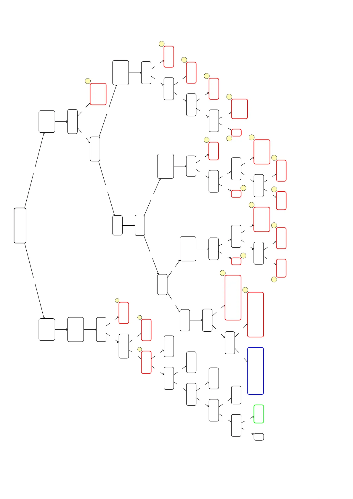
Scalar Lie p oin t symmetries of the Standard Mo del with one or t w o real gauge singlets M. Aa. Solb erg 1 Departmen t of Structural Engineering, Norw egian Universit y of Science and T ec hnology , T rondheim, Norw ay Abstract W e presen t a classiﬁcation of all scalar Lie p oin t symmetries of the Standard Mo del with one or t wo real gauge-singlet scalars (SM+S and SM+2S). By analyz- ing the asso ciated ﬁeld equations, we iden tify all realizable and inequiv alen t Lie p oin t symmetry algebras of these mo dels, distinguishing strict v ariational, v aria- tional (including div ergence symmetries), and Euler–Lagrange cases. In addition, w e devise eﬃcient algorithms that, for an y giv en n umerical instance of the mo d- els, determine the Lie p oin t symmetry algebra in eac h of the three categories by a parameter-based decision pro cedure using aﬃne reparametrizations and simple parameter tests, thereby a v oiding explicit symmetry analysis and the need to deriv e and solve the determining equations. Finally , we prov e several relev ant general re- sults, including a c haracterization of the three disjoint types of Lie p oin t symmetry generators—strict v ariational, div ergence, and non-v ariational—for a broad class of Lagrangians with p oten tials, including the SM+S and SM+2S. 1 E-mail: marius.solb erg@n tn u.no Con ten ts 1 In tro duction 1 2 Lie symmetry analysis of PDEs 3 2.1 P oint symmetries of systems of PDEs . . . . . . . . . . . . . . . . . . . . . . 3 2.2 Prolongations of inﬁnitesimal generators . . . . . . . . . . . . . . . . . . . . . 4 2.3 V ariational symmetries . . . . . . . . . . . . . . . . . . . . . . . . . . . . . . . 5 2.4 Characterization and preserv ation of symmetry types . . . . . . . . . . . . . 7 2.4.1 Aﬃne reparametrizations . . . . . . . . . . . . . . . . . . . . . . . . . 12 3 SM+S 15 3.1 Lagrangian . . . . . . . . . . . . . . . . . . . . . . . . . . . . . . . . . . . . . . 16 3.1.1 Linear terms . . . . . . . . . . . . . . . . . . . . . . . . . . . . . . . . . 16 3.2 Solving the determining equations . . . . . . . . . . . . . . . . . . . . . . . . . 17 3.3 Nature of the symmetries . . . . . . . . . . . . . . . . . . . . . . . . . . . . . . 19 3.4 Algorithm for determining SM+S symmetry algebras . . . . . . . . . . . . . 20 4 SM+2S 20 4.1 A general Lagrangian for the SM+KS . . . . . . . . . . . . . . . . . . . . . . 20 4.2 Lagrangian and reparametrizations of the SM+2S . . . . . . . . . . . . . . . 21 4.2.1 Linear terms . . . . . . . . . . . . . . . . . . . . . . . . . . . . . . . . . 23 4.3 Determining equations . . . . . . . . . . . . . . . . . . . . . . . . . . . . . . . . 25 4.4 P arameter cases and reductions of the SM+2S p oten tial . . . . . . . . . . . 26 4.4.1 Branc h I: λ 1111 ≠ 0 , λ 1122 ≠ 0 . . . . . . . . . . . . . . . . . . . . . . . . 26 4.4.2 Branc h I I: λ 1111 = 0 , λ 1122 ≠ 0 . . . . . . . . . . . . . . . . . . . . . . . 27 4.4.3 Branc h I I I: λ 1111 ≠ 0 , λ 1122 = 0 . . . . . . . . . . . . . . . . . . . . . . . 27 4.4.4 Branc h IV: λ 1111 = λ 1122 = 0 . . . . . . . . . . . . . . . . . . . . . . . . 30 4.5 Symmetry classiﬁcation in SM+2S . . . . . . . . . . . . . . . . . . . . . . . . 37 4.5.1 Inequiv alent symmetry algebras of the ﬁeld equations . . . . . . . . 37 4.5.2 Inequiv alent v ariational symmetry algebras . . . . . . . . . . . . . . . 39 4.5.3 Inequiv alent strict v ariational symmetry algebras . . . . . . . . . . . 40 4.6 Algorithm for determining SM+2S symmetry algebras . . . . . . . . . . . . 40 5 Summary and outlo ok 41 A Completion of the reduction tree: Lea v es 13–31 42 1 In tro duction Real scalar singlet extensions of the Standard Mo del (SM) are among the simplest Higgs- p ortal scenarios, in whic h new ph ysics couples to the SM only via the Higgs sector [1–4]. They can sim ultaneously oﬀer a viable dark matter candidate and induce a strongly ﬁrst- order electrow eak phase transition, as required for successful electrow eak baryogenesis and for explaining the observ ed matter–antimatter asymmetry of the Universe [5–7]. Adding one real scalar singlet to the SM (often denoted SM+S) can pro vide a dark matter candidate if a stabilizing symmetry is imp osed, most c ommonly an un brok en Z 2 1 symmetry s → − s . In that case the renormalizable Higgs-p ortal in teraction is λ sϕ s 2 Φ † Φ, where s is the singlet and Φ the Higgs doublet. Although phenomenologically restricted, the Z 2 -symmetric SM+S remains a viable dark matter model in limited regions of parame- ter space [8]. The SM+S without imposing a Z 2 symmetry has also been considered for its impact on the electro weak phase transition and its relev ance for electro w eak baryogenesis, see e.g. [7, 9, 10]. Extensions with tw o real singlets (SM+2S) allow for a richer phenomenology and a larger set of realizable symmetry groups. The added freedom can furthermore strengthen a ﬁrst-order electrow eak phase transition and accommo date a dark matter candidate, while remaining consistent with experimental constrain ts o v er a wider region of parameter space [11, 12]. Bey ond discrete stabilizing symmetries, con tinuous global symmetries acting on the singlets ma y also lead to phenomenologically viable scenarios. F or instance, in the SM+2S an SO ( 2 ) rotation symmetry is equiv alent to describing the tw o real singlets as a single complex singlet with a global U ( 1 ) symmetry , and such scenarios can yield pseudo- Goldstone b oson dark matter when the symmetry is softly brok en [13–15]. More generally , symmetries constrain mo del building by reducing the n umber of indep enden t parameters in the scalar p oten tial, and con tinuous symmetries ma y imply conserved currents. A systematic classiﬁcation of the discrete and contin uous v ariational symmetries ad- mitted b y a mo del provides a catalogue of distinct mo del classes. V ariational (No ether) symmetries are symmetries of the action in tegral and are therefore, in the absence of quan- tum anomalies, inherited by the quantized theory . In a suitable ﬁeld basis, the resulting classes are characterized b y symmetry-imp osed relations among the parameters, whic h are stable under renormalization-group evolution and can b e explored b oth theoretically and phenomenologically . Non-v ariational (also called dynamical) symmetries are also im- p ortan t in quantum ﬁeld theory [16]. A celebrated example is electromagnetic duality , whic h is a symmetry of the Euler–Lagrange equations (i.e. the equations of motion) but not of the action; see, e.g., [17]. Among the most important symmetries are Lie p oin t symmetries, i.e. contin uous trans- formations connected to the iden tity that act on the spacetime and ﬁeld v ariables and, when prolonged to deriv atives, map solutions of the ﬁeld equations to solutions. Lie p oin t symmetries ma y b e divided in to strict v ariational (SVS), divergence (DS), and non-v ariational symmetries (NVS), where SVS and DS are v ariational symmetries. In- ﬁnitesimally , these three symmetry t yp es corresp ond to three nested Lie algebras; namely , the strict v ariational symmetry algebra (spanned by the SVS generators), the v ariational symmetry algebra (spanned b y the SVS and DS generators), and the Euler–Lagrange symmetry algebra (spanned b y the SVS, DS, and NVS generators). The latter algebra con tains all Lie p oin t symmetry generators of the ﬁeld equations. The aim of this w ork is to classify all realizable Lie p oin t symmetry algebras of the three t yp es men tioned ab o v e in the generic SM+S and SM+2S mo dels, and to pro vide practical algorithms that, for an y giv en p oin t in the parameter space of either model, determine the resulting symmetry algebras without resorting to a full explicit symmetry analysis. W e ac hieve this b y applying Lie symmetry analysis of systems of partial diﬀeren tial equations (PDEs) [18] to the mo dels’ Euler–Lagrange equations, i.e. their ﬁeld equations. This approac h w as previously applied to the tw o-Higgs-doublet mo del (2HDM) in [19], which also provides p edagogical examples and further discussion of Lie’s metho d in the context of m ulti-Higgs and particle physics mo dels. 2 Outline of the article In Sections 2.1–2.3 w e review standard Lie p oin t symmetry theory for systems of PDEs, including the connection to symmetries of the action. In Section 2.4 we establish general results for theories with scalar p otentials, culminating in a theorem that characterizes the three categories of Lie p oint symmetries for a wide class of mo dels; see Corollary 1. In Section 3 we carry out the Lie p oin t symmetry classiﬁcation of the SM+S, while Section 4 classiﬁes the Lie p oin t symmetries of the SM+2S. An eﬃcien t algorithm for determining the symmetries of a given SM+2S p oten tial is presented in Section 4.6. Finally , Section 5 contains a summary and outlo ok, and App endix A collects symmetry calculations for SM+2S parameter cases that do not lead to additional symmetries. Con v entions and notation In this article we adopt the mathematicians’ con ven tion for Lie algebras, in which the generators are chosen so that [ X , Y ] ∈ g (rather than [ X , Y ] = iZ with Z ∈ g ). Moreov er, d µ ≡ d  dx µ denotes the total deriv ativ e, while D µ is reserv ed for the co v ariant deriv ativ e (3.2), unless the index is a m ulti-index J , see section 2.2. The relation g ≅ h will mean that the tw o Lie algebras are isomorphic as abstract algebras, while g ≂ O h is stronger and means that the tw o algebras are equiv alent and hence act iden tically on the ﬁelds (the singlets) after an aﬃne reparametrization with orthogonal linear part has b een p erformed. Symbols such as a ( n ) will b e used to denote sp eciﬁc realizations of algebras b y vector ﬁelds on the scalar ﬁeld space, rather than the corresp onding abstract Lie algebras. Finally , rep eated indices are implicitly summed o ver (Einstein’s summation con ven tion). 2 Lie symmetry analysis of PDEs In this section w e review the aspects of Lie symmetry theory for systems of PDEs that are relev ant for our analysis. The presen tation in Sections 2.1–2.3 partly o verlaps with our earlier review in [19], but the treatmen t here is condensed, with a few p oints elab orated. The underlying material is standard; see, e.g., [20–24]. 2.1 P oin t symmetries of systems of PDEs Consider an n th–order system of PDEs ∆ i ( x, y , y ( 1 ) , . . . , y ( n ) ) = 0 , i = 1 , . . . , m, (2.1) with d indep enden t v ariables x = ( x 0 , . . . , x d − 1 ) and q dep endent v ariables y = ( y 1 , . . . , y q ) . Here y ( k ) collectiv ely denotes all k th–order partial deriv ativ es of the y j with resp ect to the x µ . W e write the system compactly as ∆ = 0. A p oint symmetry S of (2.1) is a diﬀeomorphism of the space of indep enden t and dep enden t v ariables (a p oin t transformation) that maps solutions to solutions: S ∶ U ⊂ R d + q → R d + q , S ( x, y ) = ( ˆ x, ˆ y ) , (2.2) for some op en set U , where its action is prolonged to the deriv ativ es so that S  B k y i B x µ 1 ⋯ B x µ k  = B k ˆ y i B ˆ x µ 1 ⋯ B ˆ x µ k , (2.3) 3 and the transformed system ∆ i ( ˆ x, ˆ y , ˆ y ( 1 ) , . . . , ˆ y ( n ) ) = 0 , i = 1 , . . . , m, (2.4) holds whenev er (2.1) holds. In compact notation, ∆ = 0 ⇒ ˆ ∆ = 0 , (2.5) where ˆ ∆ ≡ ∆ ( ˆ x, ˆ y , ˆ y ( 1 ) , . . . , ˆ y ( n ) ) . 2.2 Prolongations of inﬁnitesimal generators An inﬁnitesimal generator of a p oin t transformation is a v ector ﬁeld X = ξ µ ( x, y ) B µ + η i ( x, y ) B y i , (2.6) with B µ ≡ B x µ , µ = 0 , . . . , d − 1 and i = 1 , . . . , q . The one-parameter group S ϵ = exp ( ϵX ) generated b y X acts on z = ( x, y ) by S ϵ ( z ) = ˆ z = z + ϵX ( z ) + O ( ϵ 2 ) , (2.7) for  ϵ  < ϵ 0 , where ϵ 0 > 0 ma y b e ﬁnite or inﬁnite. The k th prolongation of X extends the action of X to deriv ativ es of y up to order k , pr ( k ) X = X +  1 ≤ ∣ J ∣ ≤ k η i J B y i J , (2.8) where J = ( j 0 , . . . , j d − 1 ) is a multi–index of length  J  and y i J is the deriv ative with resp ect to J ;  J  = j 0 + ⋯ + j d − 1 , (2.9) y i J ≡ B ∣ J ∣ y i ( B x 0 ) j 0 ⋯ ( B x d − 1 ) j d − 1 . (2.10) The prolonged co eﬃcien ts η i J are giv en by η i J = D J ( Q i ) + ξ µ y i J,µ , (2.11) D J =  d dx 0  j 0 ⋯  d dx d − 1  j d − 1 , (2.12) Q i = η i − ξ µ y i ,µ , (2.13) where d  dx µ denotes the total deriv ativ e and Q i is kno wn as the char acteristic of X . A t this stage X is a candidate p oin t symmetry generator; it b ecomes a symmetry generator only after imp osing the symmetry condition (2.5). If ξ µ = 0 for all µ , the v ector ﬁeld X is in evolutionary form , X = X Q ≡ Q i B y i . (2.14) The vector ﬁeld X Q is called the evolutionary r epr esentative of X . If Q dep ends on deriv atives, then X Q is a generalized (non-p oin t) v ector ﬁeld [20]. 4 Throughout this w ork we restrict to sc alar Lie p oint tr ansformations , i.e. p oint trans- formations that lea ve the indep enden t v ariables ﬁxed. Hence ξ = 0 and Q i = η i = η i ( x, y ) , (2.15) so that X is a p oin t vector ﬁeld in ev olutionary form. F or v ector ﬁelds in evo lutionary form, the prolongation simpliﬁes to pr X = pr X Q =  i,J ( D J Q i ) B y i J =  i,J ( D J η i ) B y i J . (2.16) W e moreo ver deﬁne the (formal) inﬁnite prolongation pr X ≡ pr ( ∞ ) X (2.17) b y (2.8) with k = ∞ . Let no w G b e a connected Lie group with Lie algebra g , acting at least lo cally (i.e., p ossibly only deﬁned in a neighbourho o d of the iden tity) on the v ariables z = ( x, y ) of a fully regular (lo cally solv able with non-v anishing Jacobian) system of m PDEs ∆ = 0. Then it can b e shown that G is a (lo cal) symmetry group of ∆ = 0 if and only if  pr X ( ∆ i )  ∆ = 0 = 0 , ∀ i ∈ { 1 , . . . , m } , (2.18) for all inﬁnitesimal generators X ∈ g . In practice, only the prolongation up to the system order n is needed, i.e. pr ( n ) X . The condition (2.18) is the line arize d symmetry c ondition , and the resulting equations are the determining e quations for the symmetry algebra g . Com bining (2.8) and (2.18) yields an ov erdetermined linear system of PDEs for the co eﬃcien ts ξ µ ( x, y ) and η i ( x, y ) , whic h can typically b e solved explicitly to obtain the inﬁnitesimal symmetries. In this w ork we use the Mathematica pac k age SYM [25] to compute the determining equations. 2.3 V ariational symmetries Consider the action S [ y ] =  Ω L ( x, y , . . . , y ( n ) ) dx 0 ⋯ dx d − 1 . (2.19) A one-parameter Lie p oin t transformation group S ϵ = exp ( ϵX ) is a variational (Noether) symmetry group if it leav es the action S inv ariant up to a b oundary term. Inﬁnitesimally (i.e. to ﬁrst order in ϵ ), this holds if and only if 1 pr X ( L ) + L d µ ξ µ = d µ β µ , (2.20) where β µ is a lo cal function (i.e. a function on an appropriate jet space; see e.g. [19]) and d µ denotes the total deriv ative with resp ect to x µ , d µ = B µ + y i ,µ B y i + y i ,µν B y i ,ν + ⋯ . (2.21) 1 F or strict v ariational symmetries ( β µ ≡ 0) the equiv alence also holds for ﬁnite ϵ , at least lo cally for ϵ ∈ ⟨ − ϵ 0 , ϵ 0 ⟩ where S ϵ is deﬁned, whereas the situation is in general more complicated for divergence symmetries; see Theorem 4.12 and the discussion following Def. 4.33 in [20], resp ectiv ely . Nevertheless, whenev er (2.20) holds, S ϵ yields a (lo cal) symmetry group of the asso ciated Euler–Lagrange equations; cf. Theorem 4.34 in [20]. 5 If w e can choose β µ ≡ 0, w e call X a strict variational symmetry : pr X ( L ) + L d µ ξ µ = 0 . (2.22) Otherwise, X is a diver genc e sy mmetry . In that case, the action changes b y a b oundary term to ﬁrst order in ϵ , ˆ S = S + ϵ  B Ω β µ dF µ + O ( ϵ 2 ) , (2.23) with dF µ the out ward normal surface element on the b oundary B Ω. A ﬁrst-order b oundary term in ϵ is suﬃcien t to guaran tee an on-shell conserv ed No ether curren t, cf. (2.28) b elo w, and if the b oundary term v anishes (e.g. under suitable fall-oﬀ or p erio dicit y conditions), then the action is in v ariant to ﬁrst order in ϵ . Adding a total div ergence do es not c hange the Euler–Lagrange equations: L ′ = L + d µ β µ yields the same ﬁeld equations as L . Deﬁne the Euler op erator E = ( E 1 , . . . , E q ) b y E i =  J ( − 1 ) ∣ J ∣ D J B B y i J = B B y i − d µ B B y i ,µ + ⋯ , i = 1 , . . . , q , (2.24) so that the Euler–Lagrange equations read E ( L ) = 0 . (2.25) Moreo ver, a diﬀeren tial function f is a total div ergence if and only if [20] E ( f ) = 0 . (2.26) Hence, if pr X ( L ) + L d µ ξ µ = f , then X is a divergence symmetry precisely when (2.26) holds, in whic h case f = d µ β µ for some lo cal β µ . Let g sv ar denote the Lie algebra of strict v ariational symmetry generators, g v ar the Lie algebra of all v ariational symmetry generators, i.e. those satisfying (2.20), and g EL the Lie symmetry algebra of the Euler–Lagrange equations. Then g sv ar ⊆ g v ar ⊆ g EL . (2.27) Elemen ts of g EL ∖ g v ar are called non-variational symmetry generators. W e will call a symmetry algebra (of any of the three kinds ab o ve) r e alizable if it is maximal (with resp ect to inclusion) and is admitted b y the Euler–Lagrange equations for some parameter v alues of the Lagrangian consistent with the mo del assumptions. Subalgebras are not regarded as realizable unless they o ccur as maximal symmetry algebras for some other parameter c hoice, or are maximal within a diﬀeren t symmetry class (strict v ariational, v ariational, or Euler–Lagrange) than the am bient algebra. By No ether’s theorem, v ariational symmetries yield conserv ed currents. F or a ﬁrst- order Lagrangian L ( x, y , y ( 1 ) ) , the curren t asso ciated to X = ξ µ B µ + η i B y i can b e written as j µ = ( η i − ξ ν y i ,ν ) B L B y i ,µ + ξ µ L − β µ , d µ j µ = 0 . (2.28) A t the quantum level, v ariational symmetries t ypically lift to the path in tegral provided the measure is in v ariant (i.e. in the absence of anomalies). 6 2.4 Characterization and preserv ation of symmetry t yp es In this section we characterize the diﬀerent symmetry t yp es (strict v ariational, div er- gence, and non-v ariational) and sho w that the symmetry type is preserv ed under aﬃne reparametrizations of the ﬁelds. Let L = T − V (2.29) b e the Lagrangian of a theory , where T denotes the kinetic part (the sum of the kinetic terms), while V ( φ 1 , . . . , φ m ) is a p oten tial, i.e. a real p olynomial whose v ariables φ j form a subset of the dep enden t v ariables of the theory , φ = { φ 1 , . . . , φ m } ⊂ y = { y 1 , . . . , y q } , (2.30) where, for simplicit y , we (re-)order the φ ’s ﬁrst in y , φ i ≡ y i , ∀ i ∈ { 1 , 2 , . . . , m } . (2.31) Note that φ ma y consist of any of the ﬁelds in y , although the inten tion is to take V ( φ ) = V ( ϕ ) , i.e. let V b e a scalar p oten tial. Also note that the “kinetic” part T ma y in fact consist of an y terms complementary to V . Moreo ver, w e sa y that E ( L ) = 0 has a p olynomial c onse quenc e if it implies a relation of the form p ( φ ) = 0 , (2.32) where p is a non-zero p olynomial in the same ﬁelds as the p oten tial V . F urthermore, w e deﬁne the complement φ c = y ∖ φ = { y i } q i = m + 1 ≡ { φ c j } q − m j = 1 , (2.33) i.e. all elements of y that are not in φ . W e also let the set of all spacetime deriv atives of all ﬁelds b e given by der ( y ) = { y i J  1 ≤ i ≤ q ,  J  ≥ 1 } , (2.34) and w e will assume that T is a (ﬁnite) p olynomial in the ﬁelds and their spacetime deriv atives of arbitrary order, T ∈ R { y } ≡ R [ y , y ( 1 ) , y ( 2 ) , . . . ] , (2.35) p ossibly with a constant term. Finally , V is assumed to b e a real p olynomial in the ﬁeld v ariables φ ⊂ y and to con tain no deriv atives. Th us V = V ( φ ) ∈ R [ φ ] . (2.36) Lik ewise, the notation η i ∈ R [ y ] means that η i is a real p olynomial in the v ariables y j . Finally , the adjoint F r´ echet derivative D ∗ P of an r -tuple of diﬀerential functions P = ( P 1 , . . . , P r ) is the q × r matrix diﬀeren tial op erator deﬁned b y [20] ( D ∗ P ) ij =  J ( − 1 ) ∣ J ∣ D J ○ B P j B y i J , (2.37) 7 where D J is giv en by (2.12) and acts on the pro duct of B P j  B y i J and the function to which D ∗ P is applied. Equiv alently , for any test function ψ = ( ψ 1 , . . . , ψ r ) , ( D ∗ P ψ ) i =  j,J ( − 1 ) ∣ J ∣ D J  B P j B y i J ψ j  . (2.38) W e now presen t a substantially mo diﬁed v ersion of a theorem prov ed in [19], whic h will b e useful for characterizing strict v ariational, div ergence, and non-v ariational Lie p oin t symmetries. The assumptions are c hosen to ﬁt mo dels of the t yp e NHDM+KS (i.e. N -Higgs-doublet mo dels with K singlets): In suc h theories the kinetic part T is either at least linear in deriv ativ es or at least quadratic in φ c (e.g. the NHDM gauge b oson terms, which are at least quadratic in the gauge ﬁelds when no deriv atives are present). Nev ertheless, the theorem applies to a muc h broader class of mo dels with p oten tials. Theorem 1. L et L = T − V b e a L agr angian with T ∈ R { y } and V ( φ 1 , . . . , φ m ) ∈ R [ φ ] with φ ⊂ y , and let the inﬁnitesimal gener ator X = η i ( y 1 , . . . , y q ) B y i , wher e η i ∈ R [ y ] for al l i , b e a symmetry of E ( L ) = 0 , with c onstant terms a i = η i ( 0 ) . Mor e over, let al l terms in T b e either at le ast quadr atic in elements of the set φ c or at le ast line ar in the elements of der ( y ) . Final ly, assume that the system E ( L ) = 0 has no p olynomial c onse quenc es and that V may c ontain line ar terms α i φ i . Then the fol lowing hold, (i) If pr X ( T ) = d µ β µ for some (p ossibly vanishing) diver genc e d µ β µ , then pr X ( V ) = a i α i ∈ R . (ii) If pr X ( T ) = 0 and a i α i = 0 , then X is a strict variational symmetry gener ator. (iii) If pr X ( T ) = d µ β µ for some non-vanishing diver genc e d µ β µ , or if the diver genc e is vanishing but a i α i ≠ 0 , then X is a diver genc e symmetry gener ator. Pr o of. As in the corresp onding proof in [19], we use the follo wing identit y , whic h holds in general [20]: pr X Q ( E ( L )) = E ( pr X Q ( L )) − D ∗ Q E ( L ) , (2.39) where D ∗ Q denotes the adjoint of the F r´ echet deriv ative with resp ect to the characteristic Q asso ciated with X . Since X is in evolutionary form, (2.39) yields pr X ( E ( L )) = E ( pr X ( L )) − D ∗ Q E ( L ) . (2.40) Assuming E ( L ) = 0, the left-hand side of (2.40) v anishes since X is a symmetry of E ( L ) = 0, and E ( L ) = 0 implies the last term in (2.40) v anishes as well, since total deriv ativ es of E ( L ) v anish when ev aluated on any solution of the Euler–Lagrange equations. Hence, under the assumption E ( L ) = 0, E  pr X ( L )  = 0 . (2.41) 8 Moreo ver, if w e also assume pr X ( T ) = d µ β µ , (2.42) for a (p ossibly v anishing) divergence d µ β µ , then for all i , E i ( pr X ( V )) = B B y i pr X ( V ) = 0 , (2.43) since E ( d µ β µ ) = 0. No w, (2.43) also m ust hold when E ( L ) ≠ 0, since the system E ( L ) = 0 had no p olynomial consequences. This means that pr X ( V ) = C for a constant C ∈ R , and then C = pr X ( V ) = X ( V ) = η i B y i V , (2.44) and considering y = 0 yields C = η i ( 0 )( B y i V ) y = 0 = a i α i (2.45) where α i = 0 for i > m . W e hav e thus prov ed part (i) of the theorem. Moreo ver, pr X ( L ) = pr X ( T ) − a i α i , (2.46) whic h prov es part (ii), cf. (2.22) with ξ = 0. Moreov er, (2.46) can b e written pr X ( L ) = d µ ( β µ − a i α i x µ 4 ) ≡ d µ B µ . (2.47) This prov es part (iii) provided we can show that pr X ( T ) = d µ β µ cannot b e a non-zero real constant (and hence cannot cancel a non-zero − pr X ( V ) ). Consequen tly , the strict v ariational condition pr X ( L ) = pr X ( T ) − pr X ( V ) = 0 can only b e satisﬁed if pr X ( T ) and pr X ( V ) v anish separately , and th us cannot b e fulﬁlled in the situations cov ered by (iii): As ξ = 0 the prolongation of X applied to T yields pr X ( T ) =  i,J  D J η i ( y ) B T B y i J ∈ R { y } , (2.48) whic h means that each term of the p olynomial pr X ( T ) at least con tains one factor from φ c ∪ der ( y ) b y assumption on T , that is, pr X ( T ) = φ c σ ( i ) q i + y j ˜ J ( j ) r j , (2.49) where σ ( i ) ∈ { 1 , 2 , . . . , ( q − m )} , the m ulti-index  ˜ J ( j ) ≥ 1 and q i , r j ∈ R { y } for all i, j . Indeed, if  J  ≥ 1 in (2.48), then D J η i con tains deriv atives in each term, while for  J  = 0 eac h term of B T  B y i J is at least linear in the ﬁelds φ c . Therefore, pr X ( T ) can never equal a non-v anishing constant, and hence a strict v ariational symmetry requires pr X ( T ) = 0 and pr X ( V ) = 0 separately . The follo wing Prop osition is to a large exten t a conv erse to Theorem 1: 9 Prop osition 1. L et L = T − V b e a L agr angian, wher e V ∈ R [ φ ] with φ ⊂ y , T ∈ R { y } , and let X = η i ( φ ) B y i , b e a symmetry of E ( L ) = 0 , wher e η i ∈ R [ φ ] for al l i . Denote a i = η i ( 0 ) and let α i φ i b e the (p ossibly vanishing) line ar terms of V . Mor e over, let al l terms in T b e either at le ast quadr atic in elements of the set φ c or at le ast line ar in the elements of der ( y ) . Then the fol lowing hold: (i) If X is a strict variational symmetry gener ator, then pr X ( T ) = 0 and pr X ( V ) = a i α i = 0 . (ii) If X is a diver genc e symmetry gener ator, then pr X ( T ) is a total diver genc e, that is, pr X ( T ) = d µ β µ , while pr X ( V ) = a i α i ∈ R . Her e d µ β µ do es not c ontain a c onstant term, and d µ β µ and a i α i c annot b e simultane ously vanishing. Pr o of. In b oth cases, pr X ( V ) = X ( V ) = η i ( φ ) B V B y i ∈ R [ φ ] , (2.50) is an ordinary , real p olynomial in the v ariables φ . On the other hand, since ξ = 0 the prolongation of X applied to T yields pr X ( T ) =  i,J  D J η i ( φ ) B T B y i J ∈ R { y } , (2.51) whic h, as in the pro of of Theorem 1, means that eac h term of the p olynomial pr X ( T ) at least con tains one factor from φ c ∪ der ( y ) , that is, pr X ( T ) = φ c σ ( i ) q i + y j ˜ J ( j ) r j , (2.52) where σ ( i ) ∈ { 1 , 2 , . . . , ( q − m )} , the m ulti-index  ˜ J ( j ) ≥ 1 and q i , r j ∈ R { y } for all i, j . Th us, comparing eqs. (2.50) and (2.52), there can b e no cancellations b et w een the terms of pr X ( V ) and pr X ( T ) . In case (i), w e hav e pr X ( L ) = 0, since X is a strict v ariational symmetry , with ξ = 0, cf. (2.22). Then, in the absence of cancellations b et w een pr X ( T ) and pr X ( V ) , they must b e annihilated separately , i.e. pr X ( T ) = pr X ( V ) = 0 . (2.53) F or case (ii), assume X is a divergence symmetry . Then the total div ergence pr X ( L ) = d µ B µ ∈ R { y } , (2.54) will b e a non-zero, p olynomial function in R { y } . W e will now sho w that since pr X ( L ) equals a total div ergence, the p oten tial V cannot con tribute with more than a constan t C to pr X ( L ) , that is, pr X ( V ) = C : pr X ( L ) is a total divergence if and only if E i ( pr X ( L )) =  B B y i − d µ  B B y i ,µ  + d µ d ν  B B y i ,µν  − ⋯  pr X ( L ) = 0 , (2.55) 10 for all i , cf. (2.26), where d µ is giv en by (2.21). Hence, B pr X ( V ) B y i = 0 , (2.56) for all i , which is eviden t for i > m = dim ( φ ) since pr X ( V ) only dep ends on the ﬁelds φ . In case i ≤ m (and hence B  B y i = B  B φ i ) (2.56) also has to hold, for if the expression w as non-zero, it could not hav e b een canceled by an y other term in (2.55), since all other terms then are prop ortional to v ariables φ c or deriv ativ es, as spacetime v ariables do not o ccur explicitly in L and the total deriv atives d ξ of (2.55) hence will generate deriv ativ es in eac h term. Therefore, pr X ( V ) = C ∈ R , (2.57) whic h implies pr X ( T ) = d µ β µ ≡ d µ ( B µ + C x µ 4 ) , (2.58) where B µ w as giv en in (2.54). As giv en b y (2.52), pr X ( T ) cannot con tain a constan t term (hence, the constant C in (2.58) must b e canceled b y another term in B µ ). F urthermore, d µ β µ and C cannot b oth b e v anishing, since we then w ould ha ve a strict v ariational symmetry , con trary to our assumption. Finally , (2.50), (2.53) and (2.57) with all ﬁelds set to zero yields (for b oth cases) pr X ( V ) = η i ( 0 ) B y i ( V ) y = 0 = a i α i , (2.59) whic h concludes the pro of. W e now state and prov e a corollary that characterizes the three types of scalar Lie p oin t symmetries, again under assumptions tailored to mo dels of the type NHDM+KS. Ho wev er, the result applies more generally to evolutionary symmetries b ey ond the scalar case. Corollary 1. L et L = T − V b e a L agr angian, wher e V ∈ R [ φ ] with φ ⊂ y , T ∈ R { y } , and let X = η i ( φ ) B y i , b e a symmetry of E ( L ) = 0 , wher e η i ∈ R [ φ ] for al l i . Denote a i = η i ( 0 ) and let α i φ i b e the (p ossibly vanishing) line ar terms of V . Assume mor e over that T is such that every term is either at le ast quadr atic in elements of the set φ c or at le ast line ar in elements of der ( y ) , and that the system E ( L ) = 0 has no p olynomial c onse quenc es. Then the fol lowing hold: (i) X is a strict variational symmetry gener ator if and only if pr X ( T ) = 0 and a i α i = 0 . (ii) X is a diver genc e symmetry gener ator if and only if pr X ( T ) = d µ β µ for some β µ , and at le ast one of the c onditions pr X ( T ) = 0 and a i α i = 0 fails, i.e. ( d µ β µ ≠ 0 ) or ( a i α i ≠ 0 ) . (iii) If X is a variational symmetry gener ator, then pr X ( V ) = a i α i . 11 (iv) X is a non-variational symmetry gener ator if and only if E ( pr X ( T )) ≠ 0 . Pr o of. (i) and (ii): The righ tw ard implications follow from Prop osition 1, while the left- w ard implications follo w from Theorem 1. (iii) follows from Prop osition 1. F or (iv), w e b y (i) and (ii) kno w that the symmetry X has to be non-v ariational if and only if pr X ( T ) cannot b e written as a total divergence, which is equiv alen t to E ( pr X ( T )) ≠ 0, cf. (2.26). In Corollary 1 we did not include pr X ( V ) = a i α i on the right-hand side of the equiv- alences in (i) and (ii), since pr X ( V ) = a i α i w ould then app ear as a condition to b e pro ved every time we apply the leftw ard implications of (i) and (ii). This is not the case, as pr X ( V ) = a i α i follo ws from b oth sides of the t wo equiv alences (i) and (ii); cf. Prop osition 1 and Theorem 1. 2.4.1 Aﬃne reparametrizations In the next prop osition, w e sho w that aﬃne ﬁeld reparametrizations preserve the symme- try algebra and, moreo ver, preserve the symmetry t yp e: strict v ariational (SVS), diver- gence (DS), and non-v ariational symmetries (NVS). Prop osition 2 (Aﬃne reparametrizations) . L et ˜ y = Ay + γ (2.60) b e an aﬃne r ep ar ametrization of the ﬁelds, wher e A is a r e al, invertible q × q matrix and γ ∈ R q . Deﬁne the r ep ar ametrize d L agr angian ˜ L by ˜ L  x, ˜ y , ˜ y ( 1 ) , . . . , ˜ y ( n )  = L  x, y , y ( 1 ) , . . . , y ( n )  , (2.61) wher e y = A − 1 ( ˜ y − γ ) . Then X = ξ µ B µ + η i B y i (2.62) is a p oint symmetry of E ( L ) = 0 if and only if ˜ X = ξ µ B µ + ˜ η i B ˜ y i , ˜ η i = A ij η j , (2.63) is a p oint symmetry of ˜ E ( ˜ L ) = 0 . Mor e over, X and ˜ X ar e of the same symmetry typ e (SVS/DS/NVS), and any symmetry algebr a g = span ( X 1 , . . . , X n ) is mapp e d to an isomor- phic algebr a ˜ g = span ( ˜ X 1 , . . . , ˜ X n ) , wher e θ ( X ) = ˜ X deﬁnes a Lie algebr a isomorphism. Pr o of. Assume that X is a p oin t symmetry of E ( L ) = 0. By the chain rule applied to (2.60), B ˜ y i = B y k B ˜ y i B y k = A − 1 ki B y k . (2.64) Hence, with ˜ η i = A ij η j , ˜ X = ξ µ B µ + ˜ η i B ˜ y i = ξ µ B µ + A ij η j A − 1 ki B y k = ξ µ B µ + η k B y k = X . (2.65) 12 Th us X and ˜ X represen t the same vector ﬁeld expressed in the ( x, y ) and ( x, ˜ y ) co ordi- nates, resp ectiv ely . Since A is constan t, (2.60) and (2.63) extend to all deriv ativ es: ˜ y i J = A ij y j J , ˜ η i J = A ij η j J , (2.66) for all m ulti-indices J . Consequently , B ˜ y i J = A − 1 ki B y k J , (2.67) and the prolongations coincide, pr ˜ X = pr X , (2.68) cf. (2.8). Let ˜ E denote the Euler op erator with resp ect to the ﬁelds ˜ y . Then the Euler operators E i transform as ˜ E i = A − 1 ki E k ⇐ ⇒ ˜ E = A − T E , (2.69) and hence, using (2.61), ˜ E ( ˜ L ) = A − T E ( L ) . (2.70) Therefore, pr ˜ X  ˜ E ( ˜ L )   ˜ E ( ˜ L ) = 0 = pr X  A − T E ( L )   A − T E ( L ) = 0 = A − T pr X  E ( L )   E ( L ) = 0 = 0 , (2.71) since A − T is in vertible and X is a symmetry of E ( L ) = 0. Th us ˜ X is a p oin t symmetry of ˜ E ( ˜ L ) = 0. The conv erse direction follows by the same argumen t, since (2.60) is inv ertible. T o compare symmetry types, note that (2.68) and (2.61) imply pr ˜ X ( ˜ L ) = pr X ( L ) . (2.72) Hence ˜ X is a strict v ariational symmetry of ˜ L if and only if X is a strict v ariational symmetry of L by (2.22). Lik ewise, ˜ X is a divergence symmetry if and only if X is, since d µ ˜ β µ [ ˜ y ] = d µ β µ [ y ] (2.73) is a total divergence in either co ordinate system, where ˜ β µ is deﬁned by ˜ β µ [ ˜ y ] = β µ [ y ] ≡ β µ  x, y , y ( 1 ) , . . .  with y = A − 1 ( ˜ y − γ ) . Finally , deﬁne θ ∶ g → ˜ g b y θ ( X ) = ˜ X . By (2.65) we hav e ˜ X = X , and hence ˜ g = g and θ is the identit y map. Th us θ is a Lie algebra isomorphism, whic h concludes the pro of. F or practical reasons, the matrix A is usually chosen to b e orthogonal, so that the kinetic terms retain their canonical form. This is also the case for unitary reparametriza- tions of the doublets in NHDMs: a unitary transformation acting on the doublets induces an orthogonal transformation of their real comp onen t ﬁelds [26]. F or Higgs doublets, 13 constan t shifts sp oil the canonical form of the kinetic/gauge sector and are therefore usually av oided, except when expanding ab out a v acuum exp ectation v alue (VEV) after sp on taneous symmetry breaking (SSB). Consider a set of ﬁelds ϕ ⊂ y with iden tical gauge quantum num b ers. One may then p erform ﬁeld reparametrizations ˜ ϕ = Aϕ + γ , (2.74) where A is tak en (when p ossible) to preserv e the kinetic terms, and ϕ c = y ∖ ϕ denotes the complemen tary set of ﬁelds, cf. (2.33). If A preserves the kinetic form (e.g. A ∈ O ( n ) for real scalars), then the kinetic sector is unc hanged in the new basis, T [ ϕ, ϕ c ] = T [ ˜ ϕ, ϕ c ] . (2.75) The p otential is typically a p olynomial in ϕ , and can b e rewritten as a function of the new ﬁelds, V ( ϕ ) ≡ ˜ V ( ˜ ϕ ) , (2.76) so that it describ es the same theory although its explicit functional form generally changes, ˜ V ≠ V . Suc h mo dels exhibit what is commonly referred to as r ep ar ametrization fr e e dom . Multi-Higgs mo dels provide t ypical examples. W e will exploit this freedom to c ho ose con venien t bases and to av oid double coun ting of equiv alen t symmetry realizations. T o decide when tw o symmetries are equiv alent under a ﬁeld reparametrization, we m ust express the transformed co eﬃcien ts ˜ η i of Prop osition 2 in terms of the transformed ﬁeld v ariables ˜ y . All scalar Lie p oint symmetries of the mo dels considered in subsequent sections are of the form X = η i ( y ) B y i , (2.77) and will b e aﬃne, i.e. η ( y ) = B y + a, (2.78) for some constan t matrix B and constant vector a . Under the aﬃne reparametrization ˜ y = Ay + γ , (2.79) the co eﬃcien ts transform as ˜ η = Aη , and hence ˜ η = A ( B y + a ) = AB y + Aa. (2.80) Substituting y = A − 1 ( ˜ y − γ ) from (2.79) yields ˜ η ( ˜ y ) = AB A − 1 ˜ y − AB A − 1 γ + Aa. (2.81) Giv en t wo aﬃne scalar symmetries X 1 and X 2 with co eﬃcien ts ( B 1 , a 1 ) and ( B 2 , a 2 ) , resp ectiv ely , equation (2.81) shows that X 1 and X 2 are equiv alent under an aﬃne reparametriza- tion (2.79) if there exist A and γ such that B 1 = AB 2 A − 1 , a 1 = − AB 2 A − 1 γ + Aa 2 . (2.82) 14 W e call a reparametrization induced b y an orthogonal matrix A = O an ortho gonal r ep ar ametrization . F or singlets w e will only iden tify symmetries as equiv alent when they are related by an orthogonal reparametrization, since such transformations preserve the canonical form of the kinetic terms. 2 Moreo ver, prop ortional characteristics η and k η with k ∈ R ∖ { 0 } generate the same one-parameter symmetry group up to a rescaling of the group parameter. Hence, tw o aﬃne scalar symmetries are ortho gonal ly e quivalent if and only if there exist k ∈ R ∖ { 0 } , an orthogonal matrix O , and γ suc h that k B 1 = O B 2 O T , k a 1 = − O B 2 O T γ + O a 2 . (2.83) Finally , t wo p oin t symmetry algebras g and h of ∆ = 0 will b e called orthogonally equiv alent or just e quivalent , denoted g ≂ O h , (2.84) if one can b e mapp ed to the other by an orthogonal reparametrization, so that they describ e the same symmetry realization in diﬀeren t ﬁeld bases. Concretely , let h = span ( X 1 , . . . , X n ) and deﬁne ˜ h = span ( ˜ X 1 , . . . , ˜ X n ) , (2.85) where eac h ˜ X i is obtained from X i b y the reparametrization (2.79) with A = O (so ˜ h dep ends on the choice of O and γ ), and is written in the transformed v ariables, ˜ X i ( ˜ y ) = ˜ η j i ( ˜ y ) B ˜ y j . (2.86) W e then say that g and h are equiv alent if there exists an orthogonal matrix O and a shift v ector γ such that g = ˜ h  ˜ y → y . (2.87) 3 SM+S In this section we determine all Lie p oint symmetries of the Standard Mo del augmen ted b y a real scalar gauge singlet. Since the comp onen ts of the SM Higgs doublet and the singlet ﬁeld transform diﬀerently under SU ( 2 ) L , no non-trivial mixing of these scalars is exp ected, and the scalar Lie p oin t symmetries are therefore comparatively constrained. Moreo ver, aside from constan t singlet shifts and rephasings of the Higgs doublet, the mo del admits no further reparametrization freedom in the scalar sector, so the symmetry analysis is less in volv ed than e.g. in the 2HDM [19]. 2 U ( N ) reparametrizations of N Higgs doublets corresp ond to orthogonal transformations on the real comp onen t ﬁelds, but orthogonal transformations b ey ond the realiﬁcation of U ( N ) do not preserve the canonical kinetic form of NHDMs [26]. 15 3.1 Lagrangian The (scalar) SM+S Lagrangian can b e written as L SMS = − 1 4 W a µν W aµν − 1 4 B µν B µν + ( D µ Φ ) † ( D µ Φ ) + 1 2 B µ s B µ s − V ( Φ , s ) , (3.1) where the co v ariant deriv ativ e and the gauge ﬁeld strength tensors are given b y D µ Φ =  B µ + ig σ a 2 W a µ + ig ′ 1 2 B µ  Φ , (3.2) W a µν = B µ W a ν − B ν W a µ + g ϵ abc W b µ W c ν , (3.3) B µν = B µ B ν − B ν B µ , (3.4) and σ a are the P auli matrices ( a = 1 , 2 , 3). The most general, renormalizable SM+S p oten tial can then b e deﬁned as V ( Φ , s ) = − µ 2 Φ † Φ + λ ( Φ † Φ ) 2 + αs − µ s s 2 + κs 3 + λ s s 4 + κ sϕ Φ † Φ s + λ sϕ Φ † Φ s 2 . (3.5) Here, s is the real, scalar gauge singlet, while Φ is the SM Higgs doublet, Φ = 1 √ 2  ϕ 1 + iϕ 2 ϕ 3 + iϕ 4  , (3.6) where the ϕ ’s are real, scalar ﬁelds. 3.1.1 Linear terms The parameter α can in many cases b e eliminated by a constant ﬁeld shift, s → s − β , (3.7) with real β . Under (3.7), the tadp ole co eﬃcient transforms as α → ˜ α = α + 2 µ s β + 3 κβ 2 − 4 λ s β 3 . (3.8) Y et, eliminating α is not alwa ys p ossible; for instance, if µ s = κ = λ s = 0, or if λ s = 0 with 3 κα > µ 2 s , α cannot b e absorb ed and the p oten tial remains linear in s . W e therefore retain the linear term αs in (3.5). One might ob ject that suc h a tree-lev el p otential is not “ph ysical” because it lacks a global minim um. How ev er, a tree-lev el p oten tial V do es not, in general, ha ve to p os- sess a global minim um: It may b e unbounded from b elo w (while still admitting a lo cal, metastable minimum), or it may ev en lac k any stationary point, whereas the full eﬀectiv e p oten tial V eﬀ —including radiativ e corrections with logarithmic dep endence (for instance of Coleman–W ein b erg t yp e)—ma y develop a stable minim um [27–32]. Moreov er, the ab- sence of linear terms when expanding V eﬀ ab out one of its stationary p oints (e.g. the true v acuum) do es not justify discarding them in a symmetry analysis of the tree-level p oten tial V , since V need not p ossess a stationary p oint (ev en when V eﬀ do es) and, in any case, must b e expanded ab out one for the linear terms to v anish. Such an expansion, if p ossible, also alters the form of the gauge sector through the co v ariant-deriv ativ e terms; see Section 4.2.1 for further discussion. 16 3.2 Solving the determining equations W e now pro ceed b y applying SYM [25] to ﬁnd the determining equations (2.18) of the Euler–Lagrange equations E ( L SMS ) = 0 (3.9) of (3.1), cf. (2.24). There are 21 ﬁelds (16 gauge ﬁelds and 5 scalar ﬁelds) presen t in this mo del, and hence the Euler–Lagrange equations (3.9) form a system of 21 equations. Restricting to p oin t symmetries with no spacetime transformations and requiring the gauge ﬁelds to b e left inv ariant, we set ξ µ = 0 , for all 0 ≤ µ ≤ 3 , η i = 0 , for all 6 ≤ i ≤ 21 . (3.10) Moreo ver, w e restrict to symmetries with no explicit spacetime dep endence, i.e. η i = η i ( ϕ 1 , . . . , ϕ 5 ) . Then the inﬁnitesimal generator takes the form X = 5  i = 1 η i ( ϕ 1 , . . . , ϕ 5 ) B ϕ i , (3.11) where ϕ 1 , . . . , ϕ 4 denote the real doublet comp onen ts and ϕ 5 ≡ s, (3.12) so that w e are considering (purely) scalar symmetries. The simplest of the determining equations no w read B ϕ i B ϕ j η k = 0 , for all 1 ≤ i, j, k ≤ 5 (3.13) B y i η j = 0 , for all i > 5 ∧ 1 ≤ j ≤ 5 , (3.14) where y i for i > 5 denote the gauge ﬁeld v ariables, while y i ≡ ϕ i for i ≤ 5. This means that the non-zero η ’s are aﬃne in the scalar ﬁelds and indep enden t of the gauge ﬁeld v ariables y i for i > 5. Thus, η i = a i + b ij ϕ j , 1 ≤ i ≤ 5 , (3.15) with an implicit sum o ver j from 1 to 5. No w, deﬁne the following Lie algebra generators, X 1 = B s , (3.16) X 2 = s B s , (3.17) X 3 =  − α µ 2 s + 2 s  B s , for µ 2 s ≠ 0 (3.18) X Y = − ϕ 2 B ϕ 1 + ϕ 1 B ϕ 2 − ϕ 4 B ϕ 3 + ϕ 3 B ϕ 4 , (3.19) where X Y generates the U ( 1 ) Y h yp erc harge rephasing of the SM Higgs doublet, Φ ↦ e iϵ Φ (or equiv alen tly Φ ↦ e iϵY Φ, with hypercharge Y = 1 2 for the Higgs doublet, after rescaling ϵ ). Then, substituting (3.15) into the determining equations and requiring that the coeﬃcient of each distinct monomial in each equation v anish, we obtain ﬁv e solutions 17 and corresp onding Lie algebras (one of whic h is equiv alent to another under a constan t shift of s and is therefore redundan t in the reduced classiﬁcation). In the ﬁrst solution, all a i = b ij = 0, except for a 5 , b 55 ∈ R , b 12 = − b 43 = − b 21 = b 34 , (3.20) whic h means there are three free parameters, and hence the Lie algebra is 3-dimensional, namely a ( 1 ) ⊕ u ( 1 ) Y = span ( X 1 , X 2 , X Y ) , (3.21) where a ( 1 ) = span ( X 1 , X 2 ) is the 2-dimensional, non-ab elian aﬃne Lie algebra. The parameter conditions for the symmetry (3.21) are α = µ 2 s = κ sϕ = κ = λ sϕ = λ s = 0 , (3.22) whic h means the scalar singlet is a massless, free ﬁeld. F or the remaining solutions, the Lie symmetry algebras realized, together with the corresp onding parameter conditions, are sh ⊕ u ( 1 ) Y = span ( X 1 , X Y ) , α ≠ 0 , µ 2 s = κ sϕ = κ = λ sϕ = λ s = 0 , (3.23) sc ⊕ u ( 1 ) Y = span ( X 2 , X Y ) , µ 2 s ≠ 0 , α = κ sϕ = κ = λ sϕ = λ s = 0 , (3.24) sc ′ ⊕ u ( 1 ) Y = span ( X 3 , X Y ) , α, µ 2 s ≠ 0 , κ sϕ = κ = λ sϕ = λ s = 0 , (3.25) u ( 1 ) Y = span ( X Y ) , for all other parameter v alues. (3.26) Here sh , sc , and sc ′ are one-dimensional Lie algebras (each isomorphic to R ), distinguished b y their action on the singlet ﬁeld ( s -shifts versus s -scalings). Moreov er, sc ≂ O sc ′ . (3.27) (in the sense of (2.84) and Section 2.4.1), as explained b elo w. F or a p oten tial satisfying (3.25), w e may p erform a shift (3.7) with β = α ( 2 µ 2 s ) and hence eliminate α , without introducing new parameters (a new constan t term in the p oten tial is irrelev ant as it do es not surviv e in the Euler–Lagrange equations, and therefore do es not aﬀect the symmetries). 3 Hence, sc ≂ O sc ′ , i.e. the symmetries (3.24) and (3.25) are equiv alent through a shift of the ﬁeld s . Generators dep ending on p oten tial parameters, lik e X 3 in (3.18), are typical signs of redundan t symmetries due to the p oten tial not b eing maximally reduced. The remaining symmetry algebras sh ⊕ u ( 1 ) Y and sc ⊕ u ( 1 ) Y are inequiv alent since (2.83) would require k B 1 = OB 2 O T , i.e. 0 = 1, which is imp ossible. Therefore, the realiz- able, inequiv alent scalar Lie p oin t symmetry algebras in the SM+S may b e written a ( 1 ) ⊕ u ( 1 ) Y , sh ⊕ u ( 1 ) Y , sc ⊕ u ( 1 ) Y , u ( 1 ) Y . (3.28) 3 In the aﬃne form η ( s ) = B s + a (cf. (2.78)), the generators X 3 and X 2 corresp ond to ( B 1 , a 1 ) = ( 2 , − α / µ 2 s ) and ( B 2 , a 2 ) = ( 1 , 0 ) , resp ectiv ely . Equation (2.83) is satisﬁed with O = 1, k = 1 / 2, and γ = α /( 2 µ 2 s ) , showing that X 3 and X 2 are orthogonally equiv alent (i.e. related by an orthogonal aﬃne reparametrization and a rescaling of the group parameter). 18 3.3 Nature of the symmetries W e start b y calculating the eﬀect of a linear combination of the generators (3.16), (3.17), and (3.19) on the kinetic sector T , pr ( k 1 X 1 + k 2 X 2 + k 3 X Y )( T ) = k 2 B µ s B µ s, (3.29) where T = L SMS + V , cf. (3.1). By Theorem 1 (or Corollary 1), w e can conclude from (3.29) that X 1 generates a strict v ariational symmetry when α = 0 and a divergence symmetry when α ≠ 0, cf. (3.23). Here α ≡ α 5 in the general linear term α i ϕ i used e.g. in Theorem 1, where i = 1 , . . . , 5 and ϕ 5 = s for the SM+S cf. (3.6) and (3.12); moreov er a 5 = η 5 ( 0 ) = 1 for X 1 , cf. (3.16). On the other hand, X Y alw ays generates a strict v ariational symmetry , since for X Y w e hav e a i = 0 for all i , cf. (3.19) (and furthermore α i = 0 for i ≤ 4). It should not b e surprising that X 1 is strictly v ariational in the absence of a linear term, since it generates a constant shift s → s + c with c ∈ R , which lea v es the Lagrangian in v ariant for a free, massless scalar singlet s , cf. (3.21) and (3.22). Thus, for the symmetry algebra a ( 1 ) ⊕ u ( 1 ) Y , cf. (3.21), X 1 is strictly v ariational, since the conditions (3.22) require α = 0, whereas for sh ( 1 ) ⊕ u ( 1 ) Y , X 1 is a div ergence symmetry since α ≠ 0, cf. (3.23). W e cont inue by ch ecking the nature of X 2 : since E 5 ( pr X 2 ( T )) = E 5 ( B µ s B µ s ) = − 2 B µ B µ s, (3.30) where E 5 is the Euler op erator corresp onding to the ﬁeld s ≡ ϕ 5 , we can apply Corollary 1 (iv) and conclude that X 2 is a non-v ariational symmetry . As a consistency c heck, w e calculate E ( pr X 2 ( L 2 )) , where L 2 equals L SMS with param- eters given b y (3.24), and ﬁnd a non-v anishing result 4 µ 2 s s − 2 B µ B µ s in the s -comp onen t of the Euler op erator. Moreo ver, w e ﬁnd pr X 2  E ( L 2 )  E ( L 2 ) = 0 = 0 , (3.31) whic h conﬁrms that X 2 is a symmetry of the Euler–Lagrange equations of the SM+S with a free massiv e singlet s . Here pr X 2 is eﬀectiv ely the second prolongation of X 2 . W e conclude that there are four p ossible Lie p oin t symmetry algebras in the SM+S, giv en by (3.21), (3.23), (3.24), and (3.26). F or the ﬁrst algebra, only the subalgebra sh ⊕ u ( 1 ) Y = span ( X 1 , X Y ) is v ariational (it is strictly v ariational), so for the parameter case (3.22) w e hav e g EL = a ( 1 ) ⊕ u ( 1 ) Y , while g v ar = g sv ar = sh ⊕ u ( 1 ) Y . The second algebra, sh ⊕ u ( 1 ) Y , is v ariational, where one comp onen t is a divergence symmetry and the other is a strict v ariational symmetry; hence g EL = g v ar = sh ⊕ u ( 1 ) Y while g sv ar = u ( 1 ) Y , for the parameter case (3.23). The third algebra, sc ⊕ u ( 1 ) Y , is non-v ariational, although u ( 1 ) Y is v ariational, which means g EL = sc ⊕ u ( 1 ) Y while g v ar = g sv ar = u ( 1 ) Y for the parameter case (3.24). The same conclusions hold for the parameter case (3.25), since the t wo equiv alen t symmetry algebras are of the same symmetry type, cf. Prop osition 2. F or other parameters, g EL = g v ar = g sv ar = u ( 1 ) Y , cf. (3.26). Finally , if w e consider X Y to b e trivial since it is alwa ys presen t, the only non-trivial v ariational symmetry of the SM+S is the scalar shift symmetry X 1 = B s . It is a strict v ariational symmetry if α = 0, and a divergence symmetry otherwise. 19 3.4 Algorithm for determining SM+S symmetry algebras The parameter conditions asso ciated with the realizable Euler–Lagrange Lie point symme- try algebras g EL in the SM+S, cf. (3.21)–(3.26), yield a direct insp ection-based algorithm for iden tifying the symmetry conten t of a given SM+S p otential: 1. Read oﬀ the p oten tial parameters and iden tify whic h parameter constraints in (3.21)–(3.26) are satisﬁed. 2. Match the satisﬁed constraints to the corresp onding maximal algebra g EL . 3. Read oﬀ the v ariational subalgebras g v ar and g sv ar from the case-b y-case conclusions giv en at the end of Section 3.3. This yields an algorithmic iden tiﬁcation of the Lie p oint symmetry algebra of any numer- ical SM+S p oten tial, without explicit symmetry calculations. 4 SM+2S In this section we determine all scalar Lie p oin t symmetries of the Standard Mo del ex- tended by t wo real scalar singlets. As in the 2HDM, the scalar sector admits a non-trivial reparametrization freedom: Since the tw o singlets carry identical quantum num b ers, one ma y p erform an O ( 2 ) basis rotation in singlet space, in addition to p ossible constan t singlet shifts. W e will exploit this reparametrization freedom to keep the p oten tial in a suitably reduced form, whic h b oth ensures solv abilit y of the determining equations and prev ents rep eated o ccurrences of the same symmetry in diﬀerent singlet bases. 4.1 A general Lagrangian for the SM+KS W e write the SM+2S Lagrangian in a form applicable to the SM+KS for arbitrary K ∈ N real scalar gauge singlets, similar to the treatmen t in [33]. Let L SMKS = − 1 4 W a µν W aµν − 1 4 B µν B µν + ( D µ Φ ) † ( D µ Φ ) + 1 2 B µ s i B µ s i − V ( Φ , s ) , (4.1) with cov ariant deriv ativ e D µ and gauge-ﬁeld strength tensors given by (3.2), (3.3), and (3.4), and with the SM Higgs doublet deﬁned in (3.6). The most general renormalizable SM+KS p oten tial can b e written as V ( Φ , s ) = − µ 2 Φ † Φ + λ ( Φ † Φ ) 2 + α i s i −  i ≤ j m ij s i s j +  i ≤ j ≤ k κ ij k s i s j s k +  i ≤ j ≤ k ≤ l λ ij kl s i s j s k s l + κ i s i Φ † Φ +  i ≤ j λ ij s i s j Φ † Φ , (4.2) where all sums run from 1 to K . W e also note that the singlet kinetic term T s = 1 2 ( B µ s ) T ( B µ s ) , (4.3) is inv arian t under an orthogonal basis c hange O ∈ O ( K ) , i.e. a reparametrization ˜ s = O s with s = ( s 1 , . . . , s K ) T , since T s → 1 2 ( B µ ˜ s ) T ( B µ ˜ s ) = 1 2 ( B µ s ) T O T O ( B µ s ) = T s . (4.4) 20 The kinetic sector is thus preserved, and all singlets s i carry identical quantum n umbers; hence the Lagrangian written in the new basis ˜ s = O s represents the same physics, al- though the parameters of the p oten tial V are, in general, not in v ariant—in direct analogy with the reparametrization freedom of the scalar sector in the 2HDM [34]. 4.2 Lagrangian and reparametrizations of the SM+2S Henceforth w e set K = 2 in the summations in (4.2), corresp onding to the SM+2S, thereby obtaining the explicit p oten tial V ( Φ , s 1 , s 2 ) = − µ 2 Φ † Φ + λ ( Φ † Φ ) 2 + α 1 s 1 + α 2 s 2 −  m 11 s 2 1 + m 12 s 1 s 2 + m 22 s 2 2  + κ 111 s 3 1 + κ 112 s 2 1 s 2 + κ 122 s 1 s 2 2 + κ 222 s 3 2 + λ 1111 s 4 1 + λ 1112 s 3 1 s 2 + λ 1122 s 2 1 s 2 2 + λ 1222 s 1 s 3 2 + λ 2222 s 4 2 + ( κ 1 s 1 + κ 2 s 2 ) Φ † Φ +  λ 11 s 2 1 + λ 12 s 1 s 2 + λ 22 s 2 2  Φ † Φ . (4.5) W e retain the linear terms α i s i , since they cannot, in general, b e eliminated by shifts of the singlets, see Section 4.2.1. Nevertheless, we will use singlet shifts to simplify the parameterization: Under the reparametrizations ˜ s 1 = s 1 + γ 1 , ˜ s 2 = s 2 + γ 2 , (4.6) the reparametrized Lagrangian satisﬁes ˜ L [ ˜ s, s c ] = L [ s, s c ] = L [ ˜ s − γ , s c ] , (4.7) where γ = ( γ 1 , γ 2 ) T . Suppressing the tildes in the new basis, the reparametrized La- grangian is therefore obtained b y p erforming the substitutions s 1 → s 1 − γ 1 , s 2 → s 2 − γ 2 , (4.8) in the original Lagrangian L . The parameters of the p oten tial then transform as follows: α 1 → α 1 + 2 γ 1 m 11 + γ 2 m 12 + 3 γ 2 1 κ 111 + 2 γ 2 γ 1 κ 112 + γ 2 2 κ 122 − 4 γ 3 1 λ 1111 − 3 γ 2 γ 2 1 λ 1112 − 2 γ 2 2 γ 1 λ 1122 − γ 3 2 λ 1222 , (4.9) α 2 → α 2 + γ 1 m 12 + 2 γ 2 m 22 + γ 2 1 κ 112 + 2 γ 2 γ 1 κ 122 + 3 γ 2 2 κ 222 − γ 3 1 λ 1112 − 2 γ 2 γ 2 1 λ 1122 − 3 γ 2 2 γ 1 λ 1222 − 4 γ 3 2 λ 2222 , (4.10) µ 2 → µ 2 + γ 1 κ 1 + γ 2 κ 2 − γ 2 1 λ 11 − γ 1 γ 2 λ 12 − γ 2 2 λ 22 , (4.11) m 11 → m 11 + 3 γ 1 κ 111 + γ 2 κ 112 − 6 γ 2 1 λ 1111 − 3 γ 2 γ 1 λ 1112 − γ 2 2 λ 1122 , (4.12) m 12 → m 12 + 2 γ 1 κ 112 + 2 γ 2 κ 122 − 3 γ 2 1 λ 1112 − 4 γ 2 γ 1 λ 1122 − 3 γ 2 2 λ 1222 , (4.13) m 22 → m 22 + γ 1 κ 122 + 3 γ 2 κ 222 − γ 2 1 λ 1122 − 3 γ 2 γ 1 λ 1222 − 6 γ 2 2 λ 2222 , (4.14) κ 1 → κ 1 − 2 γ 1 λ 11 − γ 2 λ 12 (4.15) 21 κ 2 → κ 2 − γ 1 λ 12 − 2 γ 2 λ 22 (4.16) κ 111 → κ 111 − 4 γ 1 λ 1111 − γ 2 λ 1112 , (4.17) κ 112 → κ 112 − 3 γ 1 λ 1112 − 2 γ 2 λ 1122 , (4.18) κ 122 → κ 122 − 2 γ 1 λ 1122 − 3 γ 2 λ 1222 , (4.19) κ 222 → κ 222 − γ 1 λ 1222 − 4 γ 2 λ 2222 . (4.20) The quartic couplings are not listed here since they are in v ariant under singlet shifts. W e also note that an y tw o cubic couplings can generically b e eliminated by a suitable choice of ( γ 1 , γ 2 ) , unless the relev an t quartic couplings v anish, or unless the tw o shift-induced v ariations ∆ κ ( γ 1 , γ 2 ) are linearly dep enden t. Next, consider an O ( 2 ) basis transformation of the singlets, ˜ s ≡  ˜ s 1 ˜ s 2  =  cos θ − δ sin θ sin θ δ cos θ   s 1 s 2  ≡ O s, (4.21) where δ = ± 1, θ ∈ [ 0 , 2 π ) , and δ = − 1 yields an ortho gonal transformation with determinan t − 1. The reparametrized Lagrangian is then ˜ L [ ˜ s, s c ] = L [ s, s c ] = L [ O T ˜ s, s c ] , (4.22) and, suppressing the tildes in the new basis, it is obtained b y substituting s → O T s in the original Lagrangian L , i.e. s 1 → cos ( θ ) s 1 + sin ( θ ) s 2 , s 2 → − δ sin ( θ ) s 1 + δ cos ( θ ) s 2 . (4.23) In this case the parameters of the p oten tial transform as: α 1 → α 1 c θ − α 2 δ s θ , (4.24) α 2 → α 2 δ c θ + α 1 s θ , (4.25) m 11 → c 2 θ m 11 − δ c θ m 12 s θ + m 22 s 2 θ , (4.26) m 12 → δ c 2 θ m 12 + m 11 s 2 θ − m 22 s 2 θ , (4.27) m 22 → c 2 θ m 22 + δ c θ m 12 s θ + m 11 s 2 θ , (4.28) κ 1 → c θ κ 1 − δ κ 2 s θ , (4.29) κ 2 → δ c θ κ 2 + s θ κ 1 , (4.30) κ 111 → c 3 θ κ 111 − δ c 2 θ κ 112 s θ + c θ κ 122 s 2 θ − δ κ 222 s 3 θ , (4.31) κ 112 → 1 4 δ ( c θ + 3 c 3 θ ) κ 112 + 3 δ c θ κ 222 s 2 θ + 3 c 2 θ κ 111 s θ + 1 4 κ 122 ( s θ − 3 s 3 θ ) , (4.32) κ 122 → 1 4 ( c θ + 3 c 3 θ ) κ 122 − 3 δ c 2 θ κ 222 s θ + 3 c θ κ 111 s 2 θ − 1 4 δ κ 112 ( s θ − 3 s 3 θ ) , (4.33) κ 222 → δ c 3 θ κ 222 + δ c θ κ 112 s 2 θ + c 2 θ κ 122 s θ + κ 111 s 3 θ , (4.34) λ 11 → c 2 θ λ 11 − δ c θ λ 12 s θ + λ 22 s 2 θ , (4.35) λ 12 → δ c 2 θ λ 12 + λ 11 s 2 θ − λ 22 s 2 θ , (4.36) λ 22 → c 2 θ λ 22 + δ c θ λ 12 s θ + λ 11 s 2 θ , (4.37) λ 1111 → c 4 θ λ 1111 − δ c 3 θ λ 1112 s θ − δ c θ λ 1222 s 3 θ + c 2 θ λ 1122 s 2 θ + λ 2222 s 4 θ , (4.38) 22 λ 1112 → 1 2 δ ( c 2 θ + c 4 θ ) λ 1112 + 4 c 3 θ λ 1111 s θ − 4 c θ λ 2222 s 3 θ + δ λ 1222 s θ s 3 θ − 1 2 λ 1122 s 4 θ , (4.39) λ 1122 → 1 4 ( 3 c 4 θ + 1 ) λ 1122 + 3 4 δ λ 1112 s 4 θ − 3 4 δ λ 1222 s 4 θ + 3 2 λ 1111 s 2 2 θ + 3 2 λ 2222 s 2 2 θ , (4.40) λ 1222 → 1 2 δ ( c 2 θ + c 4 θ ) λ 1222 + 1 2 δ ( c 2 θ − c 4 θ ) λ 1112 − 4 c 3 θ λ 2222 s θ + 4 c θ λ 1111 s 3 θ + 1 2 λ 1122 s 4 θ , (4.41) λ 2222 → c 4 θ λ 2222 + δ c 3 θ λ 1222 s θ + δ c θ λ 1112 s 3 θ + c 2 θ λ 1122 s 2 θ + λ 1111 s 4 θ , (4.42) whereas µ 2 and λ are inv arian t. Since ˜ α = O α and ˜ s = O s , a rotational reparametrization lea ves the linear terms unchanged, ˜ α T ˜ s = α T s , as it should. Moreov er, since ˜ a = ˜ η ( 0 ) = O η ( 0 ) = O a for a scalar symmetry with characteristic η , it follo ws that ˜ a T ˜ α = a T α, (4.43) and hence a div ergence symmetry (with pr X ( T ) = 0) remains a div ergence symmetry under an orthogonal reparametrization, in accordance with Corollary 1(ii) and Prop osi- tion 2. The quartic coupling λ 1111 cannot alw ays b e transformed to zero; a coun ter-example is λ 1111 = λ 2222 = 1 with all other λ ij kl = 0. How ev er, λ 1112 can alwa ys b e set to zero: The transformed coupling ˜ λ 1112 , giv en by the righ t-hand side of (4.39), satisﬁes  2 π 0 ˜ λ 1112 ( θ ) dθ = 0 , (4.44) and since ˜ λ 1112 ( θ ) is contin uous, there exists θ 0 ∈  0 , 2 π  such that ˜ λ 1112 ( θ 0 ) = 0 . (4.45) The same argument applies to λ 1222 . T urning to the cubic singlet couplings, one lik ewise has ∀ i ∀ j ∀ k ∃ θ ∈ [ 0 , 2 π  ∶ ˜ κ ij k ( θ ) = 0 , (4.46) but, in general, not for the same θ for diﬀerent ( i, j, k ) . W e will b egin our reductions of the SM+2S p oten tial b y setting λ 1112 = 0. 4.2.1 Linear terms W e p erform the symmetry analysis on the tree-level p oten tial (4.5). As for the SM+S in Section 3.1.1, the ﬁeld shifts (4.6) cannot, in general, b e emplo yed to remov e all lin- ear terms for arbitrary parameter v alues; cf. (4.9) and (4.10). Indeed, eliminating the terms linear in the shifted singlets requires solving the coupled system ˜ α 1 ( γ 1 , γ 2 ) = 0 and ˜ α 2 ( γ 1 , γ 2 ) = 0, which may fail to admit any real solution in ( γ 1 , γ 2 ) even for tree-lev el p o- ten tials with extrema; see the argumen t b elo w. Symmetry analyses are carried out at tree lev el b ecause renormalization, in the absence of quantum anomalies, preserves v ariational symmetries, so that the eﬀective p oten tial V eﬀ has the same (v ariational) symmetries as V . A physical eﬀective p oten tial V eﬀ should p ossess a minim um, and if one expands all ﬁelds ab out suc h a minim um, no linear terms are present. How ever, this argumen t cannot b e used to remov e the linear terms from the tree-lev el p otential V , since it may happ en that V has no minimum while V eﬀ do es; cf. the discussion of the linear term in the SM+S 23 in Section 3.1.1. T o remain completely general, we therefore keep the linear terms in our symmetry analysis of V , just as w e did for the SM+S. Ev en if one w ere to demand that the tree-lev el p otential V ha ve a stationary p oin t, expanding about a stationary p oin t with nonzero comp onen ts along the Higgs-doublet directions ϕ i , i = 1 , . . . , 4, mo diﬁes the explicit form of the SM “kinetic” sector (including Higgs–gauge in teractions), e.g. b y generating gauge-b oson mass terms. Although the sym- metries are not destro yed (they are only “hidden”), this ﬁeld shift (an aﬃne reparametriza- tion) replaces the original linear (tadp ole) terms b y new quadratic and higher-order terms, corresp onding to mass and in teraction terms in the shifted ﬁelds. While the resulting pa- rameters are not indep enden t, they would nev ertheless increase the num b er of cases to b e considered in the symmetry analysis. F urthermore, expanding only in the singlet directions do es not, in general, remo ve all terms that are linear in the singlets. Let ϕ = ( ϕ 1 , . . . , ϕ 4 , s 1 , s 2 ) , (4.47) and supp ose V has a stationary p oint at ϕ = v . Then 0 = B V B ϕ i  ϕ = v ∀ i ∈ { 1 , . . . , 6 } . (4.48) Expanding ab out the full stationary p oin t, ϕ = ˜ ϕ + v , and deﬁning ˜ V ( ˜ ϕ ) = V ( ˜ ϕ + v ) , (4.49) yields 0 = B ˜ V B ˜ ϕ i  ˜ ϕ = 0 ∀ i ∈ { 1 , . . . , 6 } , (4.50) so in particular the terms linear in the shifted ﬁelds v anish, e.g. ˜ α 1 = 0 and ˜ α 2 = 0. On the other hand, consider a singlet-only shift w = ( 0 , 0 , 0 , 0 , v 5 , v 6 ) , i.e. ϕ = ˜ ϕ + w , and (re-)deﬁne ˜ V ( ˜ ϕ ) = V ( ˜ ϕ + w ) , (4.51) whic h is, in general, a diﬀerent function than the ˜ V deﬁned in (4.49). Then the stationary conditions (4.50) are ev aluated at ˜ ϕ = ( v 1 , v 2 , v 3 , v 4 , 0 , 0 ) , (4.52) rather than at ˜ ϕ = 0. In this case the singlet stationary conditions read, using (4.5), 0 = B ˜ V B ˜ s 1  ˜ s 1 = ˜ s 2 = 0 ˜ ϕ a = v a = ˜ α 1 + ˜ κ 1 ( Φ † Φ )  ˜ ϕ a = v a = ˜ α 1 + 1 2 ˜ κ 1 ( v 2 1 + v 2 2 + v 2 3 + v 2 4 ) , (4.53) and analogously for ˜ s 2 . Thus, unless ˜ κ i = 0 for the chosen shift, a singlet-only shift do es not force ˜ α 1 = ˜ α 2 = 0; rather, it ﬁxes ˜ α i in terms of the Higgs-doublet bac kground through (4.53). In addition, the p ortal terms ˜ κ i ˜ s i Φ † Φ generically surviv e a singlet-only shift, and the purely linear singlet terms ˜ α i ˜ s i v anish in general only when expanding ab out a stationary p oin t of the full scalar sector. 24 4.3 Determining equations As b efore, we apply SYM [25] to calculate the determining equations (2.18) of the 22 Euler-Lagrange equations E ( L SM2S ) = 0 , (4.54) one for eac h ﬁeld. W e will only study scalar symmetries, and hence set ξ = 0 , η i = 0 , ∀ i ≥ 7 , (4.55) i.e. w e are considering the inﬁnitesimal generator X = 6  i = 1 η i B ϕ i , (4.56) with the iden tiﬁcations ϕ 5 ≡ s 1 , ϕ 6 ≡ s 2 , (4.57) and where the ﬁrst four ϕ i ’s are the comp onen t ﬁelds of the SM Higgs doublet (3.6). Again, the simplest determining equations include B ϕ i B ϕ j η k = 0 , 1 ≤ i, j, k ≤ 6 , (4.58) whic h implies that η k is aﬃne in the scalar ﬁelds, η k = a k + b kℓ ϕ ℓ , 1 ≤ k , ℓ ≤ 6 . (4.59) Similar to the SM+S, the determining equations include B y j η i = 0 , i = 1 , . . . , 6 , j ≥ 7 , (4.60) so η 1 , . . . , η 6 are indep enden t of the gauge-ﬁeld v ariables y j . Here y j denotes the full set of ﬁeld v ariables; for j ≤ 6 we hav e y j ≡ ϕ j , while y j with j ≥ 7 are the gauge-ﬁeld v ariables. In an y case, w e restrict atten tion to scalar symmetries only and therefore do not consider gauge-ﬁeld-dep enden t generators. Then, substituting (4.59) into the determining equations and solving only the subset that is indep enden t of the p oten tial parameters (i.e. contains no parameters from V ) yields a i = 0 , i = 1 , . . . , 4 , (4.61) b j k = 0 , ( j, k ) ∉ {( 1 , 2 ) , ( 2 , 1 ) , ( 3 , 4 ) , ( 4 , 3 ) , ( 5 , 5 ) , ( 5 , 6 ) , ( 6 , 5 ) , ( 6 , 6 )} , (4.62) where, at this stage, a 5 , a 6 , b 55 , b 56 , b 65 , b 66 ∈ R , (4.63) b 12 = − b 21 = − b 43 = b 34 ∈ R . (4.64) Substituting these results into the remaining determining equations leav es the undeter- mined constan ts B 3 = { a 5 , a 6 , b 55 , b 56 , b 65 , b 66 } (4.65) app earing in the equations. The v alues and m utual relations of these constan ts may b e further restricted when the classifying equations (i.e. the determining equations con taining parameters from V ) are imp osed; in particular, they ma y set some of them to zero or yield additional equalities. One additional constan t, whic h we tak e to b e b 34 , remains undetermined but do es not o ccur in the remaining equations; it corresp onds to the ever- presen t symmetry X Y . 25 4.4 P arameter cases and reductions of the SM+2S p oten tial T o av oid unnecessary rep etitions of equiv alent Lie symmetry algebras, including “exotic” cases (i.e. instances where the symmetry generators dep end explicitly on the p oten tial parameters) and to mak e the determining equations solv able, we will reduce the p oten tial and divide our analysis into four branches. The starting p oin t for all branches is the elimination of λ 1112 , λ 1112 → 0 , (4.66) b y an SO ( 2 ) reparametrization of the p oten tial, cf. (4.45). The four branc hes are then determined by whether λ 1111 and λ 1122 v anish or not (four p ossible com binations) in the reparametrized p oten tial where λ 1112 = 0. 4.4.1 Branc h I: λ 1111 ≠ 0 , λ 1122 ≠ 0 W e now assume λ 1111 ≠ 0 , λ 1122 ≠ 0 . (4.67) Then w e can eliminate the parameters κ 111 and κ 112 b y tw o shifts (4.8), cf. (4.17) and (4.18), without altering any of the parameters λ ij kl , since they are not aﬀected by such shifts. Thus κ 111 → 0 , κ 112 → 0 . (4.68) Leaf 1 Hence, the reparametrization freedom is exhausted, and we hav e arrived at Leaf 1 in Fig. 1, highligh ted in red. By solving the determining equations with the assumptions (4.66), (4.67) and (4.68) by Mathematica ’s built-in Reduce function, we obtain t wo solutions for the parameters B 3 (4.65). The ﬁrst solution is a 5 = a 6 = b 55 = b 66 = 0 , b 56 = − b 65 , (4.69) with the parameter conditions (4.71). In addition, one parameter (taken to b e b 34 ) is free, as men tioned b elo w (4.65). Substituting (4.69) into (4.59) and (4.56) yields the follo wing symmetry algebra: so ( 2 ) ⊕ u ( 1 ) Y = span ( s 2 B s 1 − s 1 B s 2 , X Y ) , (4.70) for α 1 = α 2 = m 12 = κ 1 = κ 2 = κ 122 = κ 222 = λ 12 = λ 1222 = 0 , m 11 = m 22 , λ 11 = λ 22 , λ 1111 = λ 2222 , λ 1122 = 2 λ 2222 . (4.71) Here X Y w as given in (3.19), and so ( 2 ) ≅ R generates a rotation. The conditions (4.71) are in addition to (4.66), (4.67) and (4.68), and corresp ond to the p oten tial V = m 11 s T s + λ 11 s T s Φ † Φ + λ 1111 ( s T s ) 2 − µ 2 Φ † Φ + λ ( Φ † Φ ) 2 , (4.72) with s T = ( s 1 , s 2 ) , which indeed is inv ariant under SO ( 2 ) rotations. Since the kinetic terms are also inv arian t under SO ( 2 ) , the full Lagrangian is inv arian t, and this is a strict v ariational symmetry . The other solution yields only the ubiquitous algebra u ( 1 ) Y , which is the maximal algebra in Leaf 1 for all parameter v alues not satisfying (4.71). F or instance, after elim- inating λ 1112 b y an SO ( 2 ) rotation in singlet space, supp ose that λ 1111 ≠ 0 and λ 1122 ≠ 0. Then κ 111 and κ 112 can b e eliminated b y tw o shifts. If w e then ﬁnd, e.g., that m 11 ≠ m 22 (con tradicting (4.71)), the maximal symmetry algebra is u ( 1 ) Y . 26 λ 1112 SO ( 2 ) Ð Ð Ð Ð → 0 λ 1111 ≠ 0 λ 1122 ≠ 0 κ 111 → 0 κ 112 → 0 λ 1111 = 0 λ 1122 ≠ 0 κ 112 → 0 κ 122 → 0 I I I 1 2 Figure 1: Reduction tree, Branc hes I and I I. Eac h path starting from the ro ot at the top and terminating at a leaf (marked in red) at the b ottom corresp onds to a reduced p oten tial. F or each leaf, the determining equations are solv ed and the corresp onding symmetries are deriv ed. Leaf 1 is discussed in Section 4.4.1, while Leaf 2 is treated in Section 4.4.2. 4.4.2 Branc h I I: λ 1111 = 0 , λ 1122 ≠ 0 No w consider the case λ 1111 = 0 , λ 1122 ≠ 0 . (4.73) W e can eliminate κ 112 b y an appropriate c hoice of γ 2 , and subsequently set κ 122 to zero b y an appropriate choice of γ 1 , cf. (4.18) and (4.19), resp ectiv ely . Leaf 2 This means κ 112 → 0 , κ 122 → 0 , (4.74) and the situation is given b y Leaf 2 in Fig. 1. Solving the determining equations under the assumptions of Leaf 2, i.e. (4.66), (4.73) and (4.74), we ﬁnd that all parameters of B 3 v anish, and the symmetry algebra is the ever-presen t u ( 1 ) Y = span ( X Y ) . (4.75) 4.4.3 Branc h I I I: λ 1111 ≠ 0 , λ 1122 = 0 No w supp ose λ 1111 ≠ 0 , λ 1122 = 0 , (4.76) and w e are hence on Branch I I I in Fig. 2. Since λ 1111 ≠ 0 w e may c ho ose γ 1 suc h that κ 111 → 0 , (4.77) cf. (4.17). 27 λ 1112 SO ( 2 ) Ð Ð Ð Ð → 0 λ 1111 ≠ 0 λ 1122 = 0 κ 111 → 0 ( γ 1 ﬁxed) λ 1222 = 0? λ 2222 = 0? κ 112 = 0? κ 122 = 0? κ 222 = 0? m 12 = 0? m 22 = 0? ∅ α 2 → 0 α 1 → 0 m 22 → 0 m 12 → 0 m 11 → 0 κ 222 → 0 κ 122 → 0 λ 1111 = 0 λ 1122 = 0 λ 1222 = 0? λ 2222 = 0? λ 12 → 0 λ 11 = 0? λ 22 = 0? κ 111 → 0 κ 112 = 0? κ 122 = 0? κ 222 = 0? Contin ued in Fig. 3 m 12 → 0 ( γ 2 ﬁxed) m 22 → 0 ( γ 1 ﬁxed) m 11 → 0 ( γ 2 ﬁxed) m 12 → 0 ( γ 1 ﬁxed) κ 2 → 0 ( γ 2 ﬁxed) m 11 = 0? ∅ κ 111 = 0? κ 112 = 0? α 1 → 0 m 12 → 0 m 11 → 0 ( γ 1 ﬁxed) κ 1 → 0 ( γ 1 ﬁxed) λ 22 = 0? m 22 = 0? ∅ κ 222 = 0? κ 122 = 0? α 2 → 0 m 12 → 0 m 22 → 0 ( γ 2 ﬁxed) κ 2 → 0 κ 222 → 0 ( γ 2 ﬁxed) κ 122 = 0? κ 112 = 0? κ 111 = 0? m 11 = 0? ∅ α 1 → 0 m 11 ≠ 0 m 11 → 0 m 12 → 0 m 22 → 0 κ 122 → 0 κ 222 → 0 II I yes yes yes yes yes yes yes no no no no no no no IV yes yes yes yes yes yes no no no yes no yes yes no no no yes yes no yes yes no no no no yes yes yes yes no no no no no 3 4 5 15 16 17 18 19 20 21 22 23 24 25 26 27 28 29 30 31 Figure 2: Reduction tree, Branches II I and IV. Red b o xes indicate k ey no des, n umbered sequentially (3–31). All but one of these are lea ves corresp onding to reduced p oten tials, while No de 3 represents an in termediate reduction stage. Some leav es ma y still allow further (p ossibly nonlinear) reductions. F or eac h key no de, the determining equations are solv ed and the corresp onding symmetries are deriv ed. The empty set ∅ denotes that no further reductions apply . 28 No de 3 Moreo ver, if λ 1222 = λ 2222 = 0 , (4.78) no further κ ij k can b e eliminated b y a shift in γ 2 , but w e can still try to deriv e the p ossible symmetries for No de 3, without putting any restrictions on the parameter κ 112 of No de 3, cf. Fig. 2. With these assumptions, the determining equations yield four diﬀerent solutions, where the ﬁrst is a 5 = b 55 = b 56 = b 65 = 0 , (4.79) corresp onding to the additional parameter conditions α 2 = m 12 = m 22 = κ 2 = κ 112 = κ 122 = κ 222 = λ 12 = λ 22 = 0 , (4.80) with symmetry algebra a ( 1 ) 2 ⊕ u ( 1 ) Y = span ( B s 2 , s 2 B s 2 , X Y ) , (4.81) where the index 2 of a ( 1 ) 2 corresp onds to the ﬁeld s 2 . The second solution also includes a 6 = 0 and is v alid under the same set of parameter conditions as in (4.80), except that m 22 ≠ 0. In this case the corresp onding symmetry algebra is sc 2 ⊕ u ( 1 ) Y = span ( s 2 B s 2 , X Y ) , (4.82) where sc 2 ≅ R is the scaling algebra of s 2 . The third solution, a 5 = b 55 = b 56 = b 65 = 0 , a 6 m 22 = − b 66 α 2 2 , (4.83) is t ypical of p oten tials that are not maximally reduced, since it yields a symmetry gener- ator that dep ends explicitly on the p oten tial parameters: R ⊕ u ( 1 ) Y ≅ span ( 2 s 2 − α 2 m 22 ) B s 2 , X Y  , (4.84) whic h indicates that the potential should b e reduced further, as we hav e done for the other n umbered key no des (the leav es). See also (3.18) and the subsequent discussion. Another drawbac k of intermediate reduction stages such as No de 3 is that the determin- ing equations ma y b e to o complicated to solve. The solution (4.83) is v alid under the parameter conditions m 12 = κ 2 = κ 112 = κ 122 = κ 222 = λ 12 = λ 22 = 0 , α 2 ≠ 0 . (4.85) If m 22 ≠ 0 , (4.86) w e may eliminate α 2 b y an appropriate choice of γ 2 in (4.10), i.e. α 2 → 0 , (4.87) 29 cf. the green leaf on Branch I II in Fig. 2. This do es not rein tro duce any of the v anishing parameters, cf. (4.13)–(4.20). Th us the p oten tial is equiv alent to one with α 2 = 0, and the parameter-dep enden t generator in (4.84) disapp ears. Re-solving the determining equa- tions with (4.66), (4.76), (4.78), (4.85), (4.86), and (4.87) then yields the same algebra as in solution t wo, i.e. (4.82). If instead m 22 = 0 , (4.88) an inspection of (4.83) or a re-calculation of the determining equations with (4.66), (4.76), (4.78), (4.85) and (4.88) yields the symmetry algebra sh 2 ⊕ u ( 1 ) Y = span ( B s 2 , X Y ) , (4.89) where sh 2 ≅ R is a shift algebra. Leaf 4 W e now consider the case where λ 1222 = 0 , λ 2222 ≠ 0 , (4.90) in addition to (4.76) and (4.77) (whic h holds for all leafs of Branch I II). Since λ 2222 ≠ 0 w e may set κ 222 → 0 , (4.91) b y adjusting γ 2 , cf. (4.20). W e thus arriv e at Leaf 4 in Fig. 2. Solving the determining equations for the reduced p oten tial at Leaf 4 shows that the symmetry algebra is trivial, u ( 1 ) Y . Leaf 5 F or the ﬁnal case of Branch I I I, we assume λ 1222 ≠ 0 , (4.92) and w e may set κ 122 → 0 , (4.93) b y adjusting γ 2 . Then the only solution again yields the trivial algebra u ( 1 ) Y . 4.4.4 Branc h IV: λ 1111 = λ 1122 = 0 F or the ﬁnal branch of p oten tial reductions, Branc h IV, we assume λ 1111 = λ 1122 = 0 , (4.94) cf. Figs. 2 and 3. 30 Leaf 6 F urthermore, if we assume λ 1222 = λ 2222 = 0 , (4.95) w e may set λ 12 → 0 , (4.96) through a sp eciﬁc c hoice of θ , cf. (4.36) and the fact that ∫ 2 π 0  A cos ( 2 θ ) + B sin ( 2 θ )  dθ = 0. This will not rein tro duce any λ ij kl , b ecause all of these are zero in the ﬁrst place. If w e also assume λ 11 = λ 22 = 0 , (4.97) w e can set κ 111 → 0 , (4.98) but if κ 112 = κ 122 = κ 222 = 0 , (4.99) w e can make a new c hoice for θ without introducing parameters κ ij k . F urthermore, if κ 1 = κ 2 = 0 , (4.100) w e may set m 12 → 0 , (4.101) i.e. diagonalize the mass-squared matrix of the singlets through adjusting θ . Ho wev er, if m 11 = m 22 = 0 , (4.102) w e may set α 1 → 0 , (4.103) b y a new choice of θ (or, alternatively , w e could hav e set α 2 → 0), and none of the v anishing parameters ab o v e will reapp ear. W e hav e then ended up at Leaf 6 in Fig. 3. W e can then solv e the determining equations under the parameter conditions for Leaf 6 giv en ab o v e, whic h yields tw o solutions. In the ﬁrst, all six parameters of the set B 3 are free, whic h corresp onds to the 7-dimensional symmetry algebra [35] a ( 2 ) ⊕ u ( 1 ) Y = span ( X 1 , X 2 , X 3 , X 4 , X 5 , X 6 , X Y ) , (4.104) where X 1 = B s 1 , (4.105) X 2 = s 1 B s 1 , (4.106) X 3 = s 2 B s 1 , (4.107) X 4 = B s 2 , (4.108) X 5 = s 1 B s 2 , (4.109) X 6 = s 2 B s 2 , (4.110) 31 κ 222 = 0? ( λ ij kl = 0 , λ ij = 0 , κ 1 j k = 0) κ 1 = 0 ∧ κ 2 = 0 ? m 12 → 0 ( θ ﬁxed) m 11 = 0? m 22 = 0? α 1 → 0 ( θ ﬁxed) α 2 → 0 ( γ 2 ﬁxed) α 1 → 0 ( γ 1 ﬁxed) m 22 = 0? ∅ α 2 → 0 ( γ 2 ﬁxed) κ 1 → 0, κ 2 ≠ 0 ( θ ﬁxed) m 11 = 0? m 12 = 0? ∅ α 1 → 0 ( γ 2 ﬁxed) α 1 → 0 ( γ 1 ﬁxed) m 22 → 0 ( γ 2 ﬁxed) m 11 = 0? ∅ α 1 → 0 ( γ 1 ﬁxed) y es y es y es y es no no y es no no y es y es no no no y es no 6 7 8 9 10 11 12 13 14 Figure 3: Reduction tree, Branc h IV (contin ued). Eac h path starting from the ro ot in Fig. 2 and terminating at a leaf (n um b ered and mark ed in red) corresp onds to a reduced p otential. F or each leaf, the determining equations for the reduced p oten tial are solved and the ass ociated symmetries are derived. The empty set ∅ denotes that no further reductions apply . 32 whic h holds when the additional condition α 2 = 0 , (4.111) is satisﬁed. Thus, the only parameters that need not v anish are µ, λ ∈ R , (4.112) but since they may v anish, (4.104) is also the symmetry algebra of the kinetic terms. The aﬃne algebra of the plane, a ( 2 ) (also known as aff ( 2 ) ), is the Lie algebra of the reparametrization group A ( 2 ) (or Aﬀ ( 2 ) ) of the SM+2S. This is analogous to the fact that the symmetry algebra su ( 2 ) of the kinetic terms of the t wo-Higgs-doublet model (2HDM) is the Lie algebra of its reparametrization group SU ( 2 ) , although in this case only reparametrizations that preserve the form of the kinetic terms corresp ond to symmetries, whereas A ( 2 ) will generally not preserve the form of the kinetic terms of the SM+2S, but will still corresp ond to symmetries of the Euler–Lagrange equations. W e can c heck the nature of the symmetries of the kinetic terms T (or the Lagrangian L 0 with no singlet ﬁelds in the p oten tial) b y solving pr ( k i X i )( L 0 ) = k 2 B µ s 1 B µ s 1 + k 6 B µ s 2 B µ s 2 + ( k 3 + k 5 ) B µ s 1 B µ s 2 = 0 , (4.113) whic h means that X 1 , X 4 and X 3 − X 5 (corresp onding to k 5 = − k 3 ), in addition to X Y , are strict v ariational symmetries for L 0 . Moreo ver, by computing E ( pr ( k i X i )( L 0 )) we ﬁnd that the only non-zero elemen ts are E 5 ( pr ( k i X i )( L 0 )) = − 2 k 2 B µ B µ s 1 − ( k 3 + k 5 ) B µ B µ s 2 , (4.114) E 6 ( pr ( k i X i )( L 0 )) = − 2 k 6 B µ B µ s 2 − ( k 3 + k 5 ) B µ B µ s 1 , (4.115) hence there are no divergence symmetries for L 0 , since w e get no new v alues for the parameters k i that set these expressions to zero. Ho w ever, in theories where a p oten tial with non-v anishing linear terms is presen t, the symmetries X 1 and X 4 ma y b e degraded to divergence symmetries, cf. Corollary 1 or Prop osition 3. Considering the Lagrangian L 0 with no singlet ﬁelds in the p oten tial, w e obtain g sv ar = g v ar = span ( X 1 , X 4 , X 3 − X 5 , X Y ) = e ( 2 ) ⊕ u ( 1 ) Y , (4.116) where e ( 2 ) is the Euclidean Lie algebra in t wo dimensions, 4 while g EL = span ( X 1 , . . . , X 6 , X Y ) = a ( 2 ) ⊕ u ( 1 ) Y , (4.117) cf. (2.27). An explicit calculation of pr  k i X i   E ( L 0 )  for this mo del yields expressions con taining only terms prop ortional to E i ( L 0 ) for i = 5 , 6 (i.e. corresp onding to the singlets), conﬁrming that a ( 2 ) is a symmetry algebra of the asso ciated ﬁeld equations E ( L 0 ) = 0. The other solution to the determining equations under the parameter conditions for Leaf 6, v alid when α 2 ≠ 0 , (4.118) 4 The Euclidean Lie algebra e ( 2 ) can also b e written as R 2 ⋊ so ( 2 ) , where R 2 is spanned by the tw o comm uting shift generators. 33 yields the symmetry algebra d 4 ⊕ u ( 1 ) Y = span ( X 1 , X 2 , X 4 , X 5 , X Y ) . (4.119) Here we use the notation of [36, 37]. 5 Explicit calculations of pr X ( L ) , E ( pr X ( L )) and pr X ( E ( L )) for a p oten tial where α 2 is the only non-v anishing parameter conﬁrm that X 1 is a strict v ariational symmetry , X 4 is a div ergence symmetry while X 2 and X 5 are non-v ariational symmetries of the ﬁeld equations. Leaf 7 If the parameter conditions follo w the same path in Figures 2 and 3 as that of Leaf 6, except that m 22 ≠ 0 , (4.120) in the next-to-ﬁnal no de (and hence α 1 is still undetermined), w e cannot adjust θ without c hanging the parameters m ij . How ever, we may eliminate α 2 , i.e. set α 2 → 0 , (4.121) b y c ho osing a sp eciﬁc v alue for γ 2 , without changing an y other parameter, and we end up at Leaf 7 in Fig. 3. W e then obtain tw o p ossible symmetry algebras, a ( 1 ) 1 ⊕ sc 2 ⊕ u ( 1 ) Y = span ( X 1 , X 2 , X 6 , X Y ) , α 1 = 0 , (4.122) sh 1 ⊕ sc 2 ⊕ u ( 1 ) Y = span ( X 1 , X 6 , X Y ) , α 1 ≠ 0 . (4.123) Leaf 8 Assume that the situation no w is the same as b efore (4.102) in the paragraph on Leaf 6, but that no w m 11 ≠ 0 . (4.124) Then w e can choose a γ 1 suc h that α 1 → 0 , (4.125) cf. (4.9). If we also assume m 22 = 0 , (4.126) w e end up in Leaf 8 in Fig. 3, and can ﬁnd the corresp onding symmetries by solving the determining equations for the parameter conditions describ ed ab o ve. The tw o solutions corresp ond to symmetry algebras sc 1 ⊕ a ( 1 ) 2 ⊕ u ( 1 ) Y = span ( X 2 , X 4 , X 6 , X Y ) , α 2 = 0 , (4.127) sc 1 ⊕ sh 2 ⊕ u ( 1 ) Y = span ( X 2 , X 4 , X Y ) , α 2 ≠ 0 . (4.128) 5 The solv able Lie algebra d 4 can also b e written as R 2 ⋊ a ( 1 ) , where R 2 again is generated b y the tw o shift symmetries. 34 Leaf 9 Assume conditions identical as for Leaf 8, only with m 22 ≠ 0 , (4.129) cf. (4.126). W e may then choose a γ 2 suc h that α 2 → 0 , (4.130) as implied b y Leaf 9 in Fig. 3. The corresp onding symmetries are gl ( 2 , R ) ⊕ u ( 1 ) Y = span ( X 2 , X 3 , X 5 , X 6 , X Y ) , m 11 = m 22 , (4.131) sc 1 ⊕ sc 2 ⊕ u ( 1 ) Y = span ( X 2 , X 6 , X Y ) , m 11 ≠ m 22 . (4.132) An explicit calculation of pr X ( L ) and E ( pr X ( L )) for the case (4.131), with X = ∑ i ∈ σ k i X i and σ = { 2 , 3 , 5 , 6 } , sho ws that the only v ariational subalgebra of gl ( 2 , R ) is the one- dimensional algebra spanned by ( X 3 − X 5 ) (and this generator is strictly v ariational). Moreo ver, ev aluating pr X ( E ( L )) yields only terms prop ortional to E i ( L ) for i corre- sp onding to the singlets, conﬁrming that gl ( 2 , R ) is a symmetry algebra of the ﬁeld equations. Leaf 10 Let the parameter conditions b e as ab o v e (4.100) for Leaf 6, that is, λ ij kl = λ mn = κ opq = 0 , (4.133) for all indices, but no w assume that (4.100) do es not hold, i.e. at least one κ i is non-zero. Then w e can choose a θ such that κ 1 → 0 , κ 2 ≠ 0 . (4.134) Subsequen tly , assume m 11 = m 12 = 0 , (4.135) and w e arrive at Leaf 10 in Fig. 3. The corresp onding symmetries are then a ( 1 ) 1 ⊕ u ( 1 ) Y = span ( X 1 , X 2 , X Y ) , α 1 = 0 , (4.136) sh 1 ⊕ u ( 1 ) Y = span ( X 1 , X Y ) , α 1 ≠ 0 . (4.137) Leaf 11 Assume exactly the same parameter conditions as for Leaf 10, but with m 12 ≠ 0 . (4.138) W e may then pic k a γ 2 suc h that α 1 → 0 , (4.139) whic h corresponds to the path of parameter assumptions leading to Leaf 11. The resulting symmetry algebra is then just u ( 1 ) Y . 35 Leaf 12 Assume the same parameter conditions as for Leaf 10, only with m 11 ≠ 0 , m 12 ∈ R , (4.140) whic h means there are no assumptions on m 12 . Since m 11 ≠ 0 we ma y shift s 1 , i.e. c ho ose a γ 1 suc h that α 1 → 0 , (4.141) whic h corresp onds to Leaf 12. Then the symmetries are given b y sc 1 ⊕ u ( 1 ) Y = span ( X 2 , X Y ) , m 12 = 0 , (4.142) u ( 1 ) Y = span ( X Y ) , m 12 ≠ 0 . (4.143) Lea ves 13–31 of the reduction tree, sho wn in Figs. 2–3, do not yield an y new symmetry algebras b eyond those already app earing in Leav es 1–12, and are therefore presented in App endix A. The follo wing proposition determines the v ariational symmetry generators that emerge from the analysis of the reduction tree: Prop osition 3. Al l symmetry algebr as g that ar e r e alizable in the SM+2S ar e sub algebr as of the symmetry algebr a of the kinetic terms, a ( 2 ) ⊕ u ( 1 ) Y = span ( X 1 , . . . , X 6 , X Y ) . Mor e- over, al l elements of any r e alizable symmetry algebr a g in the SM+2S ar e non-variational, exc ept for (i) X 1 = B s 1 , which is a strict variational symmetry if α 1 = 0 , and a diver genc e symmetry if α 1 ≠ 0 . (ii) X 4 = B s 2 , which is a strict variational symmetry if α 2 = 0 , and a diver genc e symmetry if α 2 ≠ 0 . (iii) X 3 − X 5 = s 2 B s 1 − s 1 B s 2 , which is always a strict variational symmetry. (iv) X Y = − ϕ 2 B ϕ 1 + ϕ 1 B ϕ 2 − ϕ 4 B ϕ 3 + ϕ 3 B ϕ 4 , which is always a strict variational symmetry. Pr o of. Insp ecting the results from all lea ves sho ws that all realized symmetry algebras are subalgebras of a ( 2 ) ⊕ u ( 1 ) Y . F or v ariational symmetries, this also follo ws a priori from Prop osition 1. All realized symmetry algebras may b e written as the span of some of the elemen ts in the set ℵ = { X 1 , . . . , X 6 , X Y , X 3 − X 5 } . (4.144) The calculations in (4.113)–(4.115) show ed that X 1 , X 4 , and X 3 − X 5 w ere the only strict v ariational symmetries of the kinetic terms of the SM+2S, while the other elemen ts of ℵ were non-v ariational, except for X Y . The symmetry X Y is strictly v ariational for any SM+2S, indep enden t of the exact p oten tial V . By Corollary 1(i) (or Theorem 1(i)), X 3 − X 5 is strictly v ariational, since pr ( X 3 − X 5 )( T ) = 0 by (4.113) and a 1 = a 2 = 0, as there are no shifts (i.e. no X 1 or X 4 ) in volv ed in the generator. Moreo ver, b ecause X 1 and X 4 are strict v ariational symmetries of the kinetic terms, w e hav e pr X i ( T ) = 0 for i = 1 , 4. Since a 1 = 1 and a 2 = 0 for X 1 , Corollary 1(i),(ii) sho ws that X 1 is strictly v ariational if α 1 = 0 and a div ergence symmetry if α 1 ≠ 0. F or X 4 , a = ( 0 , 1 ) T , and Corollary 1(i),(ii) yields, in the same manner, that X 4 is strictly v ariational if α 2 = 0 and a div ergence symmetry if α 2 ≠ 0. 36 4.5 Symmetry classiﬁcation in SM+2S Orthogonal aﬃne reparametrizations ˜ s = O s + γ , where O is orthogonal, preserve the canonical form of the kinetic terms. W e denote symmetry generators and symmetry alge- bras that can b e mapped in to each other under such reparametrizations as (orthogonally) equiv alent; cf. Section 2.4.1. The equiv alence (or non-equiv alence) of the symmetry alge- bras found in Section 4.4 can then b e decided b y the follo wing principles, in addition to Prop osition 3 ab o ve: • Equiv alen t symmetry algebras must b e isomorphic (in particular, they must ha ve the same dimension); cf. Prop osition 2. • A symmetry generator X is mapp ed to a symmetry generator ˜ X of the same type (SVS/DS/NVS); cf. Prop osition 2. • Consider an aﬃne scalar symmetry of the form η = B s + a . Under orthogonal reparametrizations ˜ s = O s + γ , the corresp onding pairs ( B , a ) transform according to (2.83). F or conv enience, we restate (2.83): k B 1 = O B 2 O T , k a 1 = − O B 2 O T γ + O a 2 . Hence orthogonally equiv alen t linear parts are related by orthogonal similarity up to the ov erall factor k , implying that rank ( B ) is preserved, and that the eigenv alues agree up to the same prop ortionalit y factor k . 4.5.1 Inequiv alen t symmetry algebras of the ﬁeld equations W e no w consider the inequiv alen t Euler–Lagrange symmetry algebras g EL that are realized b y some SM+2S mo del. As w e hav e seen, there are man y mo dels for whic h the trivial u ( 1 ) Y algebra is the maximal symmetry algebra. The realizable, non-trivial maximal symmetry algebras of the SM+2S are as follo ws: (1+1)d algebras In the following, we suppress the ubiquitous u ( 1 ) Y summand, which is presen t in all symmetry algebras. There are then ﬁv e possible ( 1 + 1 ) d algebras, speciﬁed b y their non-trivial 1d summands, sh 1 , sh 2 , sc 1 , sc 2 , so ( 2 ) . (4.145) F or sh 1 and sh 2 , the corresp onding matrices B i ( i = 1 , 2) b oth v anish (and b oth symmetries are v ariational; cf. Prop osition 3). Moreov er, for sh 2 w e hav e η 2 = a 2 = ( 0 , 1 ) T . Since a 1 = ( 1 , 0 ) T = O a 2 , (4.146) cf. (2.83) with k = 1 (and γ arbitrary), for O =  0 1 − 1 0  , (4.147) 37 the t wo symmetries are orthogonally equiv alent. That is, sh 2 is mapp ed to sh 1 under the reparametrization deﬁned b y O , and w e write sh 1 ≂ O sh 2 ≂ O sh , (4.148) where sh is used as a common represen tative. The algebras sc 1 and sc 2 are b oth non-v ariational; cf. Prop osition 3. The corresp onding matrices B 1 =  1 0 0 0  , B 2 =  0 0 0 1  , (4.149) ha ve the same sp ectrum { 0 , 1 } (and hence prop ortional sp ectra for k = 1), whic h is a necessary condition for orthogonal equiv alence. In fact, they are orthogonally equiv alen t, since B 1 = O B 2 O T , (4.150) with a = γ = 0 and O giv en in (4.147); cf. (2.83) with k = 1. Th us, sc 1 ≂ O sc 2 ≂ O sc . (4.151) In con trast, sc  O sh : for sh one has B = 0, whereas for sc the matrix B has a nonzero eigen v alue, so the sp ectra cannot b e prop ortional. Moreov er, sh is v ariational while sc is non-v ariational. The last ( 1 + 1 ) d algebra has a non-trivial summand so ( 2 ) , and cannot b e equiv alen t to an y of the other algebras, since the corresp onding matrix is B so ( 2 ) =  0 1 − 1 0  , (4.152) with eigenv alues λ = ± i , which cannot b e prop ortional (for an y k ∈ R ) to the real eigenv al- ues o ccurring in the other ( 1 + 1 ) d cases. Hence, the three p ossible inequiv alen t ( 1 + 1 ) d symmetry algebras of the SM+2S are sh ⊕ u ( 1 ) Y , sc ⊕ u ( 1 ) Y , so ( 2 ) ⊕ u ( 1 ) Y . (4.153) Note that all algebras in (4.153) are abstractly isomorphic to R 2 , but they induce inequiv- alen t actions on the ﬁelds (up to orthogonal aﬃne reparametrizations), and are therefore not equiv alent. (2+1)d algebras Omitting the ubiquitous u ( 1 ) Y summand, the p ossible ( 2 + 1 ) d alge- bras are a ( 1 ) 1 , a ( 1 ) 2 , sh 1 ⊕ sc 2 , sc 1 ⊕ sh 2 , sc 1 ⊕ sc 2 . (4.154) The only candidates for equiv alence are the pair a ( 1 ) i (they are mutually isomorphic, but not isomorphic to the remaining algebras), and the pair of algebras of the form sh ⊕ sc , since they eac h contain one v ariational and one non-v ariational summand; cf. Prop osition 3. 38 No w, the matrix O given in (4.147), with k = 1 and γ = a = 0, maps B 2 to B 1 , cf. (4.150), and hence maps the scaling generator s 2 B s 2 to s 1 B s 1 . Moreo ver, the same c hoice of O , k , and γ maps the shift generator B s 2 to B s 1 b y (4.146). Hence, a ( 1 ) 1 ≂ O a ( 1 ) 2 . (4.155) The tw o algebras of the form sh ⊕ sc are equiv alent in a similar manner: With the same O and γ = 0 one has B s 2 ↦ B s 1 and s 1 B s 1 ↦ s 2 B s 2 , hence sh 1 ⊕ sc 2 ≂ O sc 1 ⊕ sh 2 . (4.156) Th us, there are three inequiv alent realizable ( 2 + 1 ) d symmetry algebras in the SM+2S, a ( 1 ) 1 ⊕ u ( 1 ) Y , sh 1 ⊕ sc 2 ⊕ u ( 1 ) Y , sc 1 ⊕ sc 2 ⊕ u ( 1 ) Y . (4.157) W e retain the indices to av oid confusion with other implemen tations of the same abstract Lie-algebra t yp e, e.g. a ( 1 ) = span ( s 1 B s 1 , s 1 B s 2 ) . (3+1)d algebras In our analysis, we found only one ( 3 + 1 ) d algebra of Euler–Lagrange t yp e, namely a ( 1 ) 1 ⊕ sc 2 ⊕ u ( 1 ) Y . (4.158) (4+1)d algebras W e found tw o ( 4 + 1 ) d algebras, d 4 ⊕ u ( 1 ) Y , gl ( 2 , R ) ⊕ u ( 1 ) Y , (4.159) whic h are inequiv alen t since they are not isomorphic. Moreov er, d 4 con tains t wo v aria- tional generators, whereas gl ( 2 , R ) contains none. (6+1)d algebras There are no ( 5 + 1 ) d symmetry algebras in the SM+2S. Ho wev er, there is a ( 6 + 1 ) d algebra, namely the symmetry algebra of the kinetic terms, a ( 2 ) ⊕ u ( 1 ) Y . (4.160) 4.5.2 Inequiv alen t v ariational symmetry algebras According to Proposition 3, the v ariational symmetry generators are X 1 , X 4 , X 3 − X 5 , and X Y . Hence, the realizable v ariational symmetry algebras g v ar are precisely the subalgebras generated by these elements (with u ( 1 ) Y = span ( X Y ) presen t in all cases). Insp ecting the realized symmetry algebras of the Euler–Lagrange equations listed in Section 4.5.1, we conclude that the only p ossible inequiv alent v ariational symmetry algebras of the SM+2S are sh ⊕ u ( 1 ) Y , so ( 2 ) ⊕ u ( 1 ) Y , e ( 2 ) ⊕ u ( 1 ) Y , sh 1 ⊕ sh 2 ⊕ u ( 1 ) Y . (4.161) Here, the ﬁrst t wo algebras are realized as maximal symmetry algebras for suitable pa- rameter c hoices in the SM+2S. In contrast, e ( 2 ) ⊕ u ( 1 ) Y and sh 2 ≡ sh 1 ⊕ sh 2 ≅ R 2 (4.162) only o ccur as maximal v ariational subalgebras of larger symmetry algebras of the Euler– Lagrange equations, namely a ( 2 ) and d 4 (Leaf 6), resp ectiv ely . 39 4.5.3 Inequiv alen t strict v ariational symmetry algebras W e now determine which of the v ariational symmetry algebras realized in the SM+2S, cf. (4.161), can also b e realized as strict v ariational symmetry algebras g sv ar . The algebra sh ⊕ u ( 1 ) Y exists in strict v ariational form; for instance, α 2 ma y v anish for sh 2 ⊕ u ( 1 ) Y at Leaf 3, cf. (4.89) and Proposition 3. Moreo v er, so ( 2 ) ⊕ u ( 1 ) Y is alw a ys strictly v ariational, since b oth generators are strictly v ariational; cf. Prop osition 3. The algebra e ( 2 ) ⊕ u ( 1 ) Y is the largest strict v ariational subalgebra of the symmetry algebra of the kinetic terms, as noted at Leaf 6. Finally , sh 2 ≡ sh 1 ⊕ sh 2 in (4.162) o ccurs only as a maximal v ariational subalgebra of d 4 at Leaf 6, under the condition α 2 ≠ 0. In this case, Proposition 3 implies that X 4 = B s 2 necessarily generates a divergence symmetry , so the maximal strict v ariational subalgebra of d 4 is just sh 1 . Th us, the p ossible inequiv alent maximal strict v ariational symmetry algebras realiz- able in an SM+2S mo del are sh ⊕ u ( 1 ) Y , so ( 2 ) ⊕ u ( 1 ) Y , e ( 2 ) ⊕ u ( 1 ) Y . (4.163) Only the ﬁrst tw o can coincide with the full symmetry algebra g EL of a mo del, since e ( 2 ) ⊕ u ( 1 ) Y o ccurs only as the largest strict v ariational subalgebra of g EL = a ( 2 ) ⊕ u ( 1 ) Y , the symmetry algebra of the kinetic terms; cf. Leaf 6. 4.6 Algorithm for determining SM+2S symmetry algebras Figures 1–3, together with the k ey no de/leaf analyses in Section 4.4 and App endix A, yield the following eﬃcient algorithm for determining, for any given numerical instance of an SM+2S mo del (and, in some cases, also for p oten tials with a small n umber of undetermined parameters), the maximal symmetry algebra of eac h type: 1. Start at the ro ot of Figures 1–2, and eliminate λ 1112 b y an SO ( 2 ) rotation. 2. Recompute all p oten tial parameters using eqs. (4.24)–(4.42) or eqs. (4.9)–(4.20), emplo ying the same rotation or shift as in the previous step. 3. F ollow the appropriate path in Figures 1–3 until reac hing a no de whose conten t prescrib es one or tw o reparametrizations of the form p → 0 (for some parameter p ). 4. If the no de is non-key (i.e. neither marked in red nor n umbered), p erform the pa- rameter elimination indicated at the no de via an appropriate rotation or shift, and return to Step 2. Otherwise, pro ceed. 5. At a key no de n , use the corresp onding k ey no de analysis (Leaf n for n ≠ 3, or No de 3) in Section 4.4 and App endix A to determine the admissible maximal symmetry algebra(s) g EL : If the key no de admits a unique algebra, conclude that algebra. If the key node is marked with ∅ , determine the algebra by comparing the parameters with the parameter conditions at the key no de. Otherwise, p erform the elimination indicated at the k ey no de, recompute the parameters, and determine the algebra from the recalculated p oten tial parameters. 6. Conclude that the maximal v ariational symmetry algebra g v ar for the p oten tial is generated b y g EL ∩ span ( W ) , where W = { X 1 , X 4 , X 3 − X 5 , X Y } . 40 7. Conclude that the maximal strict v ariational symmetry algebra g sv ar for the p oten tial is generated b y g EL ∩ span ( W ′ ) , where W ′ = { X 1 δ 0 ,α 1 , X 4 δ 0 ,α 2 , X 3 − X 5 , X Y } , for recalculated parameters α i . In the last step, X 1 is excluded from W ′ if the linear parameter α 1 ≠ 0, cf. Prop osition 3(i), and similarly for X 4 . F or this ﬁnal step, the parameters α i ma y sometimes hav e to b e recomputed after p erforming the elimination prescrib ed at the key no de. This is unnecessary if g EL do es not contain X 1 or X 4 . In a discrete parameter scan one will generically not satisfy exact equalities suc h as p = 0, unless p can b e eliminated by a reparametrization. One can therefore introduce a tolerance t > 0 and treat  p  < t as zero; see, e.g., [38]. 5 Summary and outlo ok W e hav e p erformed a classiﬁcation of the scalar Lie p oin t symmetries for the SM+S and SM+2S mo dels. F or the SM+S, we found four inequiv alen t realizable scalar Lie p oin t symmetry algebras g EL of the Euler–Lagrange equations, u ( 1 ) Y , sh ⊕ u ( 1 ) Y , sc ⊕ u ( 1 ) Y , a ( 1 ) ⊕ u ( 1 ) Y . (5.1) The inequiv alen t realizable v ariational scalar Lie p oin t symmetry algebras g v ar and strict v ariational scalar Lie p oin t symmetry algebras g sv ar of the SM+S w ere u ( 1 ) Y and sh ⊕ u ( 1 ) Y . (5.2) Here the shift algebra sh o ccurs as a strict v ariational symmetry algebra only when it is a subalgebra of the larger non-v ariational symmetry algebra a ( 1 ) . A simple algorithm for determining the symmetry algebras of a giv en SM+S mo del instance was provided in Section 3.4. W e found 11 inequiv alent realizable scalar Lie p oin t symmetry algebras g EL of the Euler–Lagrange equations of the SM+2S mo del. They can b e written as u ( 1 ) Y , sh ⊕ u ( 1 ) Y , sc ⊕ u ( 1 ) Y , so ( 2 ) ⊕ u ( 1 ) Y , a ( 1 ) ⊕ u ( 1 ) Y , sc 2 ⊕ u ( 1 ) Y , sh ⊕ sc ⊕ u ( 1 ) Y , a ( 1 ) ⊕ sc ⊕ u ( 1 ) Y , d 4 ⊕ u ( 1 ) Y , gl ( 2 , R ) ⊕ u ( 1 ) Y , a ( 2 ) ⊕ u ( 1 ) Y . (5.3) Some of these algebras are isomorphic as abstract Lie algebras, yet their actions on the scalar ﬁelds are inequiv alent; that is, their realizations are not related by an orthogonal aﬃne reparametrization of the scalar ﬁelds. The inequiv alent realizable v ariational scalar Lie p oin t symmetry algebras g v ar w ere u ( 1 ) Y , sh ⊕ u ( 1 ) Y , so ( 2 ) ⊕ u ( 1 ) Y , e ( 2 ) ⊕ u ( 1 ) Y , sh 2 ⊕ u ( 1 ) Y , (5.4) where the last t wo o ccur only as v ariational subalgebras of larger symmetry algebras g EL of the ﬁeld equations. 41 The inequiv alent realizable strict v ariational scalar Lie p oin t symmetry algebras g sv ar of the SM+2S w ere u ( 1 ) Y , sh ⊕ u ( 1 ) Y , so ( 2 ) ⊕ u ( 1 ) Y , e ( 2 ) ⊕ u ( 1 ) Y , (5.5) where the last algebra occurs only as a strict v ariational subalgebra of a larger symmetry algebra g EL of the ﬁeld equations. W e note that we w ould hav e missed the v ariational symmetry algebra sh 2 ⊕ u ( 1 ) Y if w e had restricted our analysis to strict v ariational sym- metries. T o distinguish b et ween diﬀerent types of symmetry generators and symmetry algebras, w e pro ved in Corollary 1 a characterization of strict v ariational (SVS), div ergence (DS), and non-v ariational (NVS) generators, v alid for a wide class of Lagrangians with p oten- tials. In Prop osition 3 w e applied this characterization to the SM+2S to determine the SVS/DS/NVS nature of its symmetry generators. Moreo ver, in Prop osition 2 we sho wed that this classiﬁcation is preserv ed under aﬃne reparametrizations. Section 4.6 furthermore presen ted an eﬃcien t algorithm for identifying the scalar Lie p oin t symmetry algebras of the SM+2S mo del for any given numerical choice of the p oten tial parameters (or, in some cases, with a few parameters left undetermined), without explicitly solving the determining equations. This parameter-based iden tiﬁcation can b e useful for n umerical parameter scans. The automorphism groups of the Lie p oin t symmetry algebras found in this w ork may b e exploited to determine the realizable discrete symmetries of the SM+S and SM+2S mo dels; see [39, 40]. Such an analysis lies outside the scop e of the present w ork. F or classiﬁcations of Lie p oin t symmetries in more complex mo dels suc h as SM+KS with K > 2, more indirect metho ds should b e considered, due to the large num b er of parameters and the resulting complexity of the reduction tree (cf. Fig. 2 for K = 2). One p ossible strategy (at least for v ariational symmetries) is to ﬁrst determine the symmetry algebra g of the kinetic terms, and then identify the realizable Lie symmetry algebras of the full Lagrangian by c ho osing one representativ e subalgebra h ⊂ g from each class of subalgebras equiv alen t under reparametrizations, and determining whether h is realizable for some c hoice of p oten tial parameters. In general, not all such subalgebras are realizable. F or instance, in the SM+2S the algebra k ⊕ u ( 1 ) Y , with the b oost k = span ( s 2 B s 1 + s 1 B s 2 ) , is not equiv alen t (under reparametrizations) to an y of the algebras (5.3)–(5.5) ab o ve (the asso ciated linear part B has eigenv alues ± 1) and is therefore not realizable. How ev er, this route w ould not yield algorithms for deciding the symmetry algebra without inv oking explicit symmetry calculations. Another approac h for mo dels with singlets is to restrict attention to tree-level p oten- tials admitting a stationary p oin t and to expand ab out suc h a p oint, thereby eliminating the singlet-linear terms. Nev ertheless, this would exclude tree-level p otentials lacking a stationary p oint ev en though the corresp onding eﬀectiv e p oten tial p ossesses a stationary p oin t (global minimum), resulting in a less general analysis. Moreo ver, expanding ab out suc h a stationary p oin t leads to a more complicated kinetic/gauge sector; see Sections 3.1.1 and 4.2.1 for a discussion of b oth cav eats. A Completion of the reduction tree: Lea v es 13–31 This app endix completes the reduction-tree analysis b y considering Lea ves 13–31, shown in Figs. 2–3. These leav es do not yield an y symmetry algebras b ey ond those already 42 app earing in Leav es 1–12. Leaf 13 Supp ose, as for Leaf 6, that λ ij kl = 0 , λ ij = 0 , κ 1 j k = 0 , (A.1) for all indices, but that κ 222 ≠ 0 . (A.2) Then w e can pick a γ 2 suc h that m 22 → 0 , (A.3) cf. (4.14). Moreov er assume m 11 = 0 . (A.4) The symmetries corresp onding to this case, given by Leaf 13, are a ( 1 ) 1 ⊕ u ( 1 ) Y = span ( X 1 , X 2 , X Y ) , κ 1 = m 12 = α 1 = 0 , (A.5) sh 1 ⊕ u ( 1 ) Y = span ( X 1 , X Y ) , κ 1 = m 12 = 0 , α 1 ≠ 0 , (A.6) u ( 1 ) Y = span ( X Y ) , for all other parameter v alues. (A.7) Leaf 14 Assume the same parameter conditions as in Leaf 13, except that m 11 ≠ 0 , (A.8) and hence w e can choose a γ 1 suc h that α 1 → 0 , (A.9) as displa yed in Leaf 14 in Fig. 3. The corresp onding symmetries are then sc 1 ⊕ u ( 1 ) Y = span ( X 2 , X Y ) , m 12 = 0 , (A.10) u ( 1 ) Y = span ( X Y ) , m 12 ≠ 0 . (A.11) Leaf 15 Now supp ose λ ij kl = 0 , λ ij = 0 , κ 111 = κ 112 = 0 , (A.12) in the same manner as for Leaf 6, but with κ 122 ≠ 0 . (A.13) Then we may ﬁrst pic k a γ 2 that eliminates m 12 , thereafter a γ 1 that eliminates m 22 without rein tro ducing m 12 , cf. (4.13) and (4.14), that is, m 12 → 0 , (A.14) m 22 → 0 , (A.15) corresp onding to Leaf 15 in Fig. 2. The s ymmetry in this case is just u ( 1 ) Y . 43 Leaf 16 Assume the parameter conditions are the same as in (A.12), with the only diﬀerence κ 112 ≠ 0 . (A.16) Then w e may ﬁrst c ho ose a γ 2 that eliminates m 11 , then pic k a γ 1 that remo ves m 12 : m 11 → 0 , (A.17) m 12 → 0 , (A.18) as sho wn in Leaf 16 in Fig. 2. The only p ossible symmetry algebra is then u ( 1 ) Y . Leaf 17 Supp ose, in the same w ay as for Leaf 6, that λ ij kl = λ 11 = λ 12 = 0 , (A.19) but, in con trast to the case for Leaf 16 (and Leaf 6), λ 22 ≠ 0 . (A.20) Then a particular c hoice for γ 2 yields κ 2 → 0 , (A.21) cf. (4.16). F urthermore, assume m 11 = 0 , (A.22) whic h leads us to Leaf 17. The symmetries in this case are then a ( 1 ) 1 ⊕ u ( 1 ) Y = span ( X 1 , X 2 , X Y ) , κ 1 = κ 111 = κ 112 = κ 122 = m 12 = α 1 = 0 , (A.23) sh 1 ⊕ u ( 1 ) Y = span ( X 1 , X Y ) , κ 1 = κ 111 = κ 112 = κ 122 = m 12 = 0 , α 1 ≠ 0 , (A.24) u ( 1 ) Y = span ( X Y ) , for all other parameter v alues . (A.25) Leaf 18 Now supp ose the parameters are the same as for Leaf 17, only with m 11 ≠ 0 . (A.26) If w e in addition assume κ 111 = κ 112 = 0 , (A.27) w e can eliminate α 1 b y a shift inv olving a sp ecial v alue of γ 1 , α 1 → 0 , (A.28) cf. (4.9), corresp onding to Leaf 18 in Fig. 2. Then the p ossible symmetries are sc 1 ⊕ u ( 1 ) Y = span ( X 2 , X Y ) , κ 1 = κ 122 = m 12 = 0 , (A.29) u ( 1 ) Y = span ( X Y ) , for all other parameter v alues . (A.30) 44 Leaf 19 W e now make the same assumptions as for Leaf 18, only with κ 112 ≠ 0 , (A.31) whic h makes it p ossible to eliminate m 12 , m 12 → 0 , (A.32) b y some choice of γ 1 , as display ed in Leaf 19 in Fig. 2. Here α 1 is undetermined, i.e. α 1 ∈ R . Then, at Leaf 19 the only admissible symmetry algebra is u ( 1 ) Y . Leaf 20 Assume, as for the tw o previous leav es, that λ ij kl = λ 11 = λ 12 = κ 2 = 0 , (A.33) whereas λ 22 , m 11 , κ 111 ≠ 0 . (A.34) Then w e can set m 11 to zero b y a choice of γ 1 , m 11 → 0 , (A.35) corresp onding to Leaf 20. The only symmetry is then u ( 1 ) Y . Leaf 21 Supp ose, as for Leaf 17, that λ ij kl = λ 12 = 0 , (A.36) for all indices, but that λ 11 ≠ 0 , (A.37) whic h allows us to set κ 1 → 0 , (A.38) b y some choice of γ 1 . Moreov er, if λ 22 = m 22 = 0 , (A.39) the situation is as giv en by Leaf 21 in Fig. 2, and we ﬁnd the follo wing symmetries: a ( 1 ) 2 ⊕ u ( 1 ) Y = span ( X 4 , X 6 , X Y ) , κ 2 = κ 112 = κ 122 = κ 222 = m 12 = α 2 = 0 , (A.40) sh 2 ⊕ u ( 1 ) Y = span ( X 4 , X Y ) , κ 2 = κ 112 = κ 122 = κ 222 = m 12 = 0 , α 2 ≠ 0 , (A.41) u ( 1 ) Y = span ( X Y ) , for all other parameter v alues . (A.42) 45 Leaf 22 Now supp ose the situation is the same as for Leaf 21, only with m 22 ≠ 0 . (A.43) Then, if κ 122 = κ 222 = 0 , (A.44) w e can set α 2 → 0 , (A.45) b y c ho osing a sp eciﬁc v alue for γ 2 , and w e arriv e at Leaf 22 in Fig. 2. Then there are t wo p ossible symmetry algebras, sc 2 ⊕ u ( 1 ) Y = span ( X 6 , X Y ) , κ 2 = κ 112 = m 12 = 0 , (A.46) u ( 1 ) Y = span ( X Y ) , for all other parameter v alues . (A.47) Leaf 23 W e now assume the same conditions as for Leaf 22, only with κ 122 ≠ 0 , (A.48) and α 2 undetermined. W e can then choose a γ 2 suc h that m 12 → 0 , (A.49) since κ 122 ≠ 0. Then the only symmetry algebra is u ( 1 ) Y . Leaf 24 Assume the same conditions as for Leaf 23, only with κ 222 ≠ 0 , (A.50) while m 12 and κ 112 are undetermined. Then we can set m 22 → 0 , (A.51) b y some choice of γ 2 , and w e end up at Leaf 24. Again, the only p ossible symmetry algebra is u ( 1 ) Y . Leaf 25 Supp ose, as for Leaf 24 and previous lea ves, λ ij kl = λ 12 = κ 1 = 0 , λ 11 ≠ 0 , (A.52) whereas λ 22 ≠ 0 , (A.53) in con trast to earlier. W e can then set κ 2 → 0 , (A.54) b y a choice of γ 2 , without altering κ 1 , since λ 12 = 0, cf. (4.15). Then there are t w o p ossible symmetry algebras, so ( 2 ) ⊕ u ( 1 ) Y = span  ( X 3 − X 5 ) , X Y  , (A.55) for κ ij k = m 12 = α i = 0 , λ 11 = λ 22 , m 11 = m 22 , (A.56) u ( 1 ) Y = span ( X Y ) , for all other parameter v alues , (A.57) where the conditions κ ij k = 0 and α i = 0 are understo od to hold for all indices i, j, k . The conditions (A.56) corresp ond to the same p oten tial as in (4.72) in Branc h I, but with λ 1111 = 0. 46 Leaf 26 Assume λ 1 ij k = 0 , λ 2222 ≠ 0 , (A.58) for all indices i, j, k . Then, by a choice of γ 2 , w e can set κ 222 → 0 . (A.59) Moreo ver, supp ose κ ij k = 0 , (A.60) for all other indices as w ell, and m 11 = 0 , (A.61) corresp onding to Leaf 26. The p ossible symmetry algebras are then a ( 1 ) 1 ⊕ u ( 1 ) Y = span ( X 1 , X 2 , X Y ) , (A.62) for λ 11 = λ 12 = κ 1 = m 12 = α 1 = 0 , sh 1 ⊕ u ( 1 ) Y = span ( X 1 , X Y ) , (A.63) for λ 11 = λ 12 = κ 1 = m 12 = 0 , α 1 ≠ 0 , u ( 1 ) Y = span ( X Y ) , for all other parameter v alues . (A.64) Leaf 27 Assume the same parameter conditions as for Leaf 26, only with m 11 ≠ 0 , (A.65) and w e can set α 1 → 0 , (A.66) b y a c hoice of γ 1 without altering m 11 , as given b y Leaf 27. The tw o p ossible symmetry algebras are then sc 1 ⊕ u ( 1 ) Y = span ( X 2 , X Y ) , λ 11 = λ 12 = κ 1 = m 12 = 0 , (A.67) u ( 1 ) Y = span ( X Y ) , for all other parameter v alues . (A.68) Leaf 28 Now, let the assumptions b e the same as for Leaf 27, only with κ 111 ≠ 0 , (A.69) and m 11 and α 1 undetermined. W e can then choose a γ 1 suc h that m 11 → 0 . (A.70) The only p ossible symmetry algebra is then u ( 1 ) Y . 47 Leaf 29 F or the next case, we make the same assumption as for Leaf 28, except that κ 112 ≠ 0 , (A.71) and the parameters κ 111 and m 11 are completely unkno wn. W e can then set m 12 → 0 , (A.72) b y some choice of γ 1 . Then the only p ossible symmetry algebra is again u ( 1 ) Y . Leaf 30 Supp ose all parameters are the same as for Leaf 29, only with κ 122 ≠ 0 , (A.73) and with no conditions on κ 112 and m 12 . By pic king an appropriate v alue of γ 1 , we can set m 22 → 0 , (A.74) and w e ﬁnd only the trivial symmetry algebra u ( 1 ) Y . Leaf 31 Finally , assume that λ 11 ij = 0 , λ 1222 ≠ 0 , (A.75) for all indices i and j . W e can then set κ 122 → 0 , κ 222 → 0 , (A.76) b y ﬁrst c ho osing an appropriate v alue of γ 2 that n ulliﬁes κ 122 and migh t also change κ 222 . Afterw ards, we can pic k a v alue of γ 1 that eliminates κ 222 without c hanging κ 122 , cf. (4.19) and (4.20). Then the only admitted Lie p oin t symmetry algebra is u ( 1 ) Y . References [1] V. Silveira and A. Zee, Sc alar phantoms , Physics L etters B 161 (1985) 136–140. [2] J. McDonald, Gauge singlet sc alars as c old dark matter. , Physic al r eview. D, Particles and ﬁelds 50 6 (1994) 3637–3649. [3] C. Burgess, M. Pospelov and T. ter V eldhuis, The minimal mo del of nonb aryonic dark matter: a singlet sc alar , Nucle ar Physics B 619 (Dec., 2001) 709–728. [4] G. Arcadi, A. Djouadi and M. Raidal, Dark matter thr ough the higgs p ortal , Physics R ep orts 842 (2020) 1–180. [5] A. Ahriche, What is the criterion for a str ong ﬁrst or der ele ctr owe ak phase tr ansition in singlet mo dels? , Physic al R eview D 75 (Apr., 2007) . [6] J. R. Espinosa, T. Konstandin and F. Riv a, Str ong El e ctr owe ak Phase T r ansitions in the Standar d Mo del with a Singlet , Nucl. Phys. B 854 (2012) 592–630, [ 1107.5441 ]. 48 [7] J. Ellis, M. Lewicki, M. Merchand, J. M. No and M. Zych, The sc alar singlet extension of the Standar d Mo del: gr avitational waves versus b aryo genesis , JHEP 01 (2023) 093, [ 2210.16305 ]. [8] Y. Y u, T.-P . T ang and L. F eng, New c onstr aints on singlet sc alar dark matter mo del with lz, invisible higgs de c ay and gamma-r ay line observations , 2025. [9] I. Lewis and M. Sulliv an, Benchmarks for double higgs pr o duction in the singlet-extende d standar d mo del at the lhc , P hysic al R eview D 96 (Aug., 2017) . [10] C.-Y. Chen, J. Kozaczuk and I. M. Lewis, Non-r esonant c ol lider signatur es of a singlet-driven ele ctr owe ak phase tr ansition , Journal of High Ener gy Physics 2017 (Aug., 2017) . [11] A. T oﬁghi, O. Gho dsi and M. Saeedhoseini, Phase tr ansition in multi-sc alar-singlet extensions of the standar d mo del , Physics L etters B 748 (Sept., 2015) 208–211. [12] V. R. Sha jiee and A. T oﬁghi, Ele ctr owe ak phase tr ansition, gr avitational waves and dark matter in two sc alar singlet extension of the standar d mo del , The Eur op e an Physic al Journal C 79 (Apr., 2019) . [13] V. Barger, P . Langack er, M. McCask ey , M. Ramsey-Musolf and G. Shaughnessy , Complex singlet extension of the standar d mo del , Phys. R ev. D 79 (Jan, 2009) 015018. [14] K. Kannike and M. Raidal, Phase T r ansitions and Gr avitational Wave T ests of Pseudo-Goldstone Dark Matter in the Softly Br oken U(1) Sc alar Singlet Mo del , Phys. R ev. D 99 (2019) 115010, [ 1901.03333 ]. [15] C. Arina, A. Beniwal, C. Degrande, J. Heisig and A. Scaﬃdi, Glob al ﬁt of pseudo-nambu-goldstone dark matter , Journal of High Ener gy Physics 2020 (Apr., 2020) . [16] D. B. Skinner, “Symmetries in quantum ﬁeld theory .” Chapter 6 of the lecture notes for Quantum Field The ory II (Univ ersity of Cambridge, P art I I I Mathematical T rip os), 2015. [17] L. Alv arez-Gaum ´ e and F. Zamora, Duality in quantum ﬁeld the ory (and string the ory) , Sept., 1997. [18] S. Lie and F. Engel, The orie der T r ansformationsgrupp en , vol. 1-3. B.G. T eubner, Leipzig, 1888-1893. [19] M. A. Solb erg, Lie symmetry analysis of the two-higgs-doublet mo del ﬁeld e quations , Physic a Scripta 101 (jan, 2026) 035209. [20] P . J. Olver, Applic ations of Lie Gr oups to Diﬀer ential Equations , vol. 107 of Gr aduate T exts in Mathematics . Springer, New Y ork, 2 ed., 1993, 10.1007/978-1-4612-4350-2. [21] P . J. Olver, “ L e ctur es on Lie Gr oups and Diﬀer ential Equations .” https://www- users.cse.umn.edu/ ~ olver/sm.html , 2012. 49 [22] P . E. Hydon, Symmetry Metho ds for Diﬀer ential Equations: A Be ginner’s Guide , v ol. 22 of Cambridge T exts in Applie d Mathematics . Cam bridge Universit y Press, Cam bridge, 2000. [23] G. W. Bluman, A. F. Cheviako v and S. C. Anco, Applic ations of Symmetry Metho ds to Partial Diﬀer ential Equations , vol. 168 of Applie d Mathematic al Scienc es . Springer, 2010. [24] B. Cant w ell, Intr o duction to Symmetry Analysis . Cam bridge T exts in Applied Mathematics. Cam bridge Universit y Press, 2002. [25] S. Dimas and D. Tsoub elis, SYM: A new symmetry-ﬁnding p ackage for Mathematic a , in The 10th international c onfer enc e in mo dern gr oup analysis , pp. 64–70, Nicosia, Univ ersity of Cyprus, 2005. [26] K. Olaussen, P . Osland and M. A. Solb erg, Symmetry and Mass De gener ation in Multi-Higgs-Doublet Mo dels , JHEP 07 (2011) 020, [ 1007.1424 ]. [27] S. Coleman and E. W einberg, R adiative c orr e ctions as the origin of sp ontane ous symmetry br e aking , Phys. R ev. D 7 (1973) 1888–1910. [28] E. Gildener and S. W einberg, Symmetry br e aking and sc alar b osons , Phys. R ev. D 13 (1976) 3333–3341. [29] J. E. Camargo-Molina, B. O’Leary , W. P oro d and F. Staub, V evacious: A to ol for ﬁnding the glob al minima of one-lo op eﬀe ctive p otentials , Eur. Phys. J. C 73 (2013) 2588, [ 1307.1477 ]. [30] F. Staub, R e op en p ar ameter r e gions in two-higgs doublet mo dels , Phys. L ett. B 776 (2018) 407–411, [ 1705.03677 ]. [31] M. E. Krauss, T. Opferkuch and F. Staub, The ultr aviolet landsc ap e of two-higgs doublet mo dels , Eur. Phys. J. C 78 (2018) 1020, [ 1807.07581 ]. [32] I. P . Iv ano v and F. V az˜ ao, Y et another lesson on the stability c onditions in multi-higgs p otentials , JHEP 11 (2020) 104, [ 2006.00036 ]. [33] T. Rob ens, T. Stefaniak and J. Wittbro dt, Two-r e al-sc alar-singlet extension of the sm: Lhc phenomenolo gy and b enchmark sc enarios , The Eur op e an Physic al Journal C 80 (F eb., 2020) . [34] G. Branco, P . F erreira, L. La voura, M. Reb elo, M. Sher and J. P . Silv a, The ory and phenomenolo gy of two-higgs-doublet mo dels , Physics R ep orts 516 (July , 2012) 1–102. [35] P . J. Olver, Equivalenc e, Invariants and Symmetry . Cambridge Universit y Press, Cam bridge, 1995, 10.1017/CBO9780511609565. [36] A. Andrada, M. L. Barb eris, I. G. Dotti and G. P . Ov ando, Pr o duct structur es on four dimensional solvable lie algebr as , Homolo gy, Homotopy and Applic ations 7 (2005) 9–37, [ math/0402234 ]. 50 [37] G. Ov ando, F our dimensional symple ctic lie algebr as , Beitr¨ age zur Algebr a und Ge ometrie 47 (2006) 419–434. [38] Plantey , R. and Solb erg, M. Aa., Computable c onditions for or der-2 CP symmetry in NHDM p otentials , JHEP 05 (2024) 260, [ 2404.02004 ]. [39] P . E. Hydon, How to use Lie symmetries to ﬁnd discr ete symmetries , in Mo dern Gr oup Analysis VII (N. H. Ibragimov, K. R. Naqvi and E. Straume, eds.), pp. 141–147. MARS Publishers, T rondheim, 1999. [40] P . Hydon, How to c onstruct the discr ete symmetries of p artial diﬀer ential e quations , Eur op e an Journal of Applie d Mathematics 11 (2000) 515–527. 51

Scalar Lie point symmetries of the Standard Model with one or two real gauge singlets

Original Paper

Comments & Academic Discussion

Leave a Comment

Original Paper

Related Papers

Comments & Academic Discussion

Leave a Comment