FGFRFT: Fast Graph Fractional FourierTransform via Fourier Series Approximation

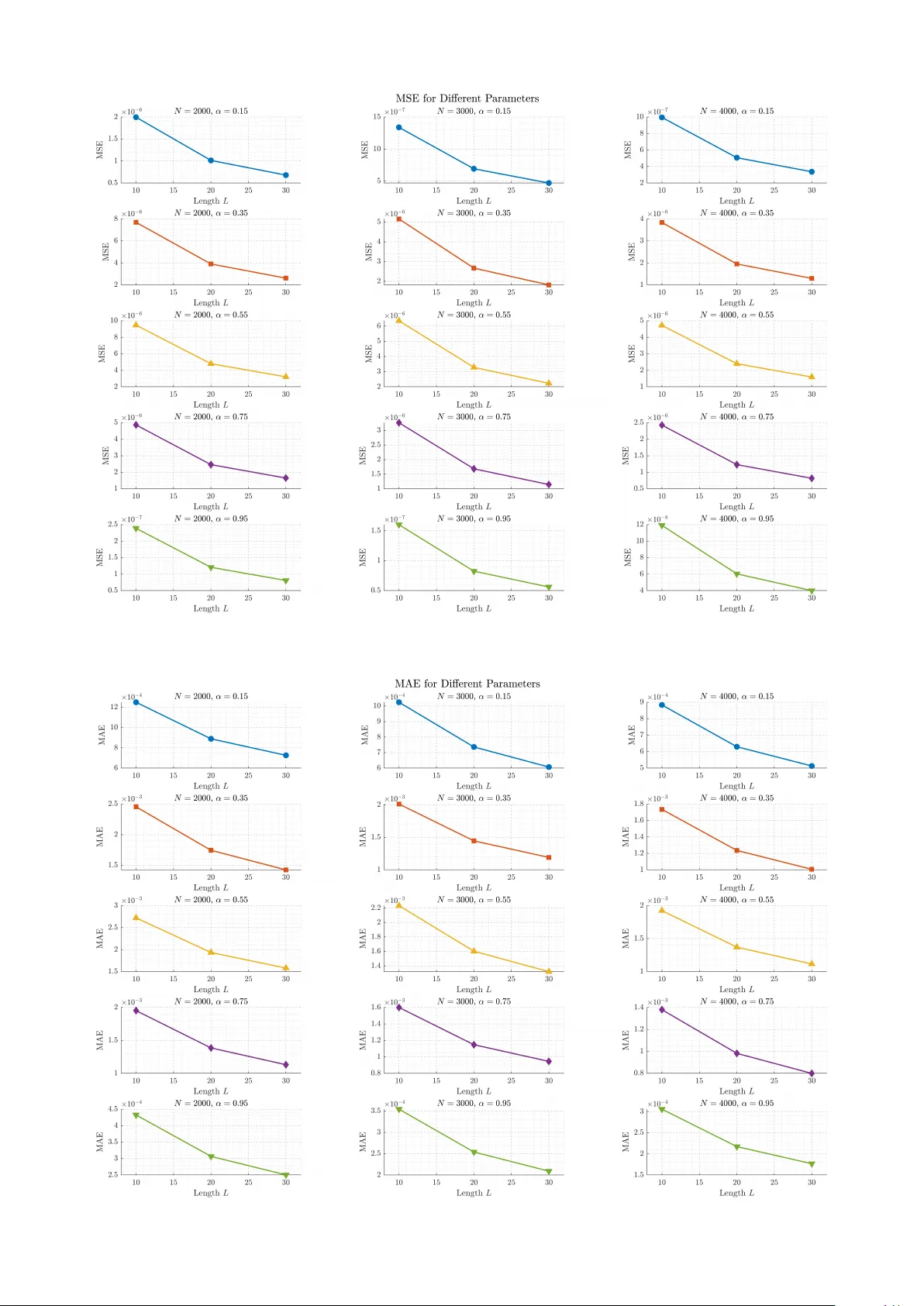
1 FGFRFT : F ast Graph Fractional F ourier T ransform via F ourier Series Approximation Ziqi Y an, Sen Shi, Feiyue Zhao, Manjun Cui, Y angfan He, and Zhichao Zhang, Member , IEEE Abstract —The graph fractional F ourier transform (GFRFT) generalizes the graph Fourier transf orm (GFT) b ut suffers from a significant computational bottleneck: determining the optimal transform order requires expensive eigendecomposi- tion and matrix multiplication, leading to O ( N 3 ) complexity . T o address this issue, we propose a fast GFRFT (FGFRFT) algorithm for unitary GFT matrices based on F ourier series approximation and an efficient caching strategy . FGFRFT reduces the complexity of generating transform matrices to O (2 LN 2 ) while preserving differentiability , thereby enabling adaptive order learning. W e validate the algorithm through theoretical analysis, approximation accuracy tests, and order learning experiments. Furthermor e, we demonstrate its prac- tical efficacy for image and point cloud denoising and pr esent the fractional specformer , which integrates the FGFRFT into the specf ormer architectur e. This integration enables the model to overcome the limitations of a fixed GFT basis and learn op- timal fractional orders for complex data. Experimental results confirm that the pr oposed algorithm significantly accelerates computation and achieves superior performance compared with the GFRFT . Index T erms —Graph signal processing, GFRFT , F ourier series approximation, FGFRFT . I . I N T R O D U C T I O N I N recent years, graph signal processing (GSP) has emerged as a powerful theoretical frame work for ana- lyzing high-dimensional data in irregular domains, such as social networks, biological systems, and sensor data [1]– [4]. It has been widely applied to tasks such as filtering, sampling, and reconstruction [5]–[11]. As the cornerstone of GSP , the graph Fourier transform (GFT) is the funda- mental tool for transforming graph signals from the vertex domain to the spectral domain. Building on this foundation, researchers have generalized the GFT to the graph fractional Fourier transform (GFRFT) by introducing the concept of transform order . The GFRFT can transform graph signals This work was supported in part by the Open Foundation of Hubei Ke y Laboratory of Applied Mathematics (Hubei University) under Grant HB AM202404; in part by the Foundation of Ke y Laboratory of System Control and Information Processing, Ministry of Education under Grant Scip20240121; and in part by the Startup Foundation for Introducing T alent of Nanjing Institute of T echnology under Grant YKJ202214. (Correspond- ing author: Zhichao Zhang.) Ziqi Y an, Sen Shi, Feiyue Zhao, and Manjun Cui are with the School of Mathematics and Statistics, Nanjing Univ ersity of Information Science and T echnology , Nanjing 210044, China (e-mail: yanziqi54@gmail.com; 202312380032@nuist.edu.cn; 202511150010@nuist.edu.cn; cmj1109@163.com). Y angfan He is with the School of Communication and Artificial In- telligence, School of Integrated Circuits, Nanjing Institute of T echnology , Nanjing 211167, China, and also with the Jiangsu Province Engineering Research Center of IntelliSense T echnology and System, Nanjing 211167, China (e-mail: Y angfan.He@njit.edu.cn). Zhichao Zhang is with the School of Mathematics and Statistics, Nanjing Univ ersity of Information Science and T echnology , Nanjing 210044, China, with the Hubei Key Laboratory of Applied Mathematics, Hubei University , W uhan 430062, China, and also with the Ke y Laboratory of System Control and Information Processing, Ministry of Education, Shanghai Jiao T ong Univ ersity , Shanghai 200240, China (e-mail: zzc910731@163.com). from the vertex domain to an intermediate domain between the vertex and spectral domains, thereby offering a more flexible approach for the representation and processing of graph signals [12]–[18]. W ang et al. first established the mathematical framework for the GFRFT based on the eigendecomposition of the graph Laplacian matrix [19]. Building on this foundation, researchers hav e verified its superiority across multiple domains. In sampling and reconstruction, W ang and Li demonstrated that, under the optimal fractional order , signal recov ery under the band-limited assumption achiev es higher accuracy than the traditional GFT [20]. In filtering and signal detection, Ozturk et al. achiev ed ef ficient signal-to- noise separation for the GFRFT -domain W iener filtering theory , whereas Cui et al. le veraged this transform to address the challenge of detecting graph linear frequency modulation signals [21], [22]. Furthermore, in data compression, Y an et al. demonstrated the advantages of fractional-domain rep- resentation for information compaction using multidimen- sional and multi-parameter GFRFT [23], [24]. Lev eraging the dual security provided by the multi-parameter space, Cui et al. pioneered new av enues for graph signal encryption and decryption [24]. Ho wev er , the determination of the transform order in these studies relies primarily on grid search strategies. T o overcome the limitations of traditional grid search in parameter determination, GFRFT is undergoing a profound shift toward a data-dri ven adaptiv e paradigm. Alikasifoglu et al. proposed an adaptiv e update strategy for the GFRFT transform order [25], laying the theoretical foundation for automated parameter optimization. On this basis, Y an et al. proposed a trainable joint time-verte x graph fractional Fourier transform, achieving end-to-end learning of opti- mal order pairs [26]. The angular GFRFT proposed by Zhao et al. demonstrated optimal denoising performance on complex data such as images and point clouds under non-stationary noise by integrating adaptiv e strategies for angle and order [27]. Subsequently , Sheng et al. advanced the integrated GFRFT with deep learning by proposing a generalized fractional-filtering embedding model that sig- nificantly improv ed performance on graph classification tasks [28]. In this context, Li et al. introduced the graph fractional Hilbert transform, which constructs precise graph- analytic signals via a parameter-adapti ve update mechanism, thereby achieving a deep alignment between the feature space and task objecti ves in speech classification [29]. This adaptiv e learning mechanism significantly enhances system robustness, thereby establishing a solid foundation for the dev elopment of intelligent and adaptive GSP systems. Despite the significant theoretical adv antages of the GFRFT , determining the optimal transform order remains a major computational bottleneck in practical applications. 2 Existing methods for order selection typically rely on grid search or gradient descent-based updates. Howe v er , these approaches require computationally expensi ve eigendecom- position and dense matrix operations for each order selection or update, resulting in computational complexity as high as O ( N 3 ) . This prohibitive computational cost not only restricts the scalability of the GFRFT on large-scale graph data but also sev erely impedes its integration as a learnable module within end-to-end deep learning frameworks. T o address this issue, focusing on unitary GFT matrices, this study proposes the FGFRFT , which combines a caching strategy with Fourier series approximation theory . This method avoids repeated eigendecomposition of the GFT matrix. By pre-caching the powers of the GFT matrix and approximating the GFRFT via Fourier series, it transforms the originally expensi ve matrix-matrix multiplications into efficient scalar-matrix linear combinations. This improve- ment reduces the computational complexity from O ( N 3 ) to O (2 LN 2 ) . Crucially , this approximation process preserves full differentiability , so the transform order need not be determined via search; instead, it can be treated directly as a network parameter, enabling end-to-end adaptiv e learning and updating during training using gradient descent. T o comprehensively ev aluate the effecti veness of the proposed algorithm, we conduct multi-faceted experimental validations. First, we analyze the numerical approximation accuracy of the algorithm and then conduct transform-order learning experiments that empirically validate its capability and con vergence in dynamically updating the transform order via gradient descent. Subsequently , in image and point cloud denoising tasks, we compare the performance of our method against the traditional GFRFT , demonstrating its dual advantages in computational ef ficiency and processing effecti v eness. Finally , to explore the algorithm’ s potential applications in deep learning, we replace the GFT module in the specformer [30] architecture with the GFRFT and FGFRFT modules, further ev aluating its compatibility and performance as a learnable component within advanced neural network models. The main contributions of this research are summarized as follo ws: • W e propose a fast approximation algorithm to mitigate the computational bottleneck of the GFRFT . By lev er- aging Fourier series approximation theory and a strate- gic caching mechanism, we successfully reduce the computational comple xity from O ( N 3 ) to O (2 LN 2 ) , making the fractional transform computationally effi- cient for large-scale graphs. • W e preserve the differentiability of the GFRFT with respect to the transform order , enabling the automatic update of the fractional order via gradient descent. This key property allows the FGFRFT to be embedded as a learnable, plug-and-play module within modern deep neural network architectures. • W e validate the effecti veness and generalization ability of the algorithm across multiple scenarios. Through numerical experiments, we verify the accuracy of the approximation and its order of con ver gence. In image and point cloud denoising tasks, we demonstrate the advantages of denoising. Furthermore, by integrating FGFRFT into the specformer architecture, we pro ve the algorithm’ s compatibility and performance improve- ment within deep learning architectures. The remainder of this research is organized as follows: Section II elaborates on the fundamental theories; Section III discusses the FGFRFT ; Section IV analyses the approx- imation accurac y and efficiency of the method; Section V presents the experimental results; and Section VI draws the conclusions of this paper . The overall framework of the research is illustrated in Fig. 1. I I . P R E L I M I NA R I E S A. GFT W e define a graph structure as G = ( V , A ) , where V = { v 1 , . . . , v N } contains N nodes. The weighted adjacency matrix A ∈ C N × N describes the connectivity relationships between nodes, where its element A m,n is non-zero if and only if there exists an edge between node n and node m ; if A m,n = 0 , it indicates no connection. T ypically , if A m,n = A n,m is satisfied, the graph is considered an undirected graph [31]. A graph signal defined on the vertices of graph G can be represented as a vector x ∈ C N . This vector establishes a mapping from the verte x set V to the comple x domain C , meaning the n -th element x n in the vector corresponds to the signal v alue on verte x v n . The definition of the GFT relies on the spectral decom- position of the graph shift operator (GSO). Let Z ∈ C N × N be a GSO of arbitrary form; common choices include the adjacency matrix A , the Laplacian matrix L , and their normalized forms [32]–[34]. The Jordan decomposition of Z can be obtained as [19]: Z = V Z J Z V Z − 1 , (1) where J Z is the Jordan normal form matrix, and the column vectors of V Z = [ v 1 , . . . , v N ] constitute the generalized eigen vectors of Z . Based on this, the GFT matrix is defined as the in verse of the eigen vector matrix, i.e., F G = V Z − 1 . For any graph signal x , its spectral representation ˜ x in the GFT domain can be calculated via the following formula: ˜ x ≜ F G x = V Z − 1 x . (2) Correspondingly , the in verse graph Fourier transform (IGFT) is used to recover the graph signal from the spectral domain to the verte x domain: x = F − 1 G ˜ x = V Z ˜ x . (3) B. GFRFT The GFRFT is a generalization of the traditional GFT , aiming to introduce the theory of fractional Fourier trans- form from classical signal processing into the graph signal domain. Given an arbitrary graph G and its GSO matrix Z , we first consider the eigendecomposition form of the unitary GFT matrix F G : F G = V − 1 Z = VΣV H , (4) where Σ is the Jordan form (diagonal eigen v alue matrix) of F G . Based on this, the GFRFT matrix with order α ∈ [0 , 1] can be defined as: F α G = VΣ α V H . (5) 3 Fig. 1: Overall framework of the paper Furthermore, to maintain consistency with the definition of classical fractional Fourier transform (FRFT) based on hyper-dif ferential operators and to support arbitrary real- number orders α ∈ R , literature [25] proposes another equiv alent definition: F α G = exp  − j απ 2  π ( D 2 G + F G D 2 G F − 1 G ) − 1 2 I N  , (6) where the operator D 2 G is gi ven by: D 2 G = 1 2 π  j 2 π log( F G ) + 1 2 I N  . (7) The above two definitions are essentially equiv alent; both satisfy inde x additi vity and possess desirable boundary prop- erties: degenerating to the identity matrix I N when α = 0 , and becoming the standard GFT matrix F G when α = 1 . C. F ourier Series Approximation Theory The Fourier series is a core mathematical tool for ana- lyzing periodic functions, stating that any periodic signal satisfying the Dirichlet conditions can be decomposed into a weighted sum of complex exponential functions [35]–[38]. For a square-integrable function g ( θ ) defined on the finite interval [ − π , π ] , we can view it as a function with a period of 2 π through periodic extension. According to the Fourier series expansion, this function can be expressed as the following complex exponential series: g ( θ ) = ∞ X n = −∞ c n e j nθ , θ ∈ [ − π , π ] , (8) where c n are the Fourier coefficients, obtained via orthog- onal projection: c n = 1 2 π Z π − π g ( θ ) e − j nθ dθ . (9) I I I . F G F R F T This section focuses on the unitary property of the GFT matrix, detailing the mathematical deriv ation of reconstruct- ing the GFRFT matrix using Fourier series approximation theory . W e deriv e the corresponding fast computation for- mulas and analyze their computational complexity . A. F ourier Series Expansion of GFRFT Eigen values Let F G be a GFT matrix that is unitary . It can be eigendecomposed as F G = VΣV H . The core operation of GFRFT in volv es performing fractional power operations on the diagonal matrix Σ after eigendecomposition, resulting in Σ α , and then re-multiplying the matrices to obtain F α G = VΣ α V H . Therefore, the GFRFT generation process requires eigen- decomposition and matrix multiplication. For the eigen- decomposition part, a caching strategy can be adopted, caching the required V , Σ , V H and only calculating Σ α to av oid repetitiv e decomposition of the GFT matrix. Howe ver , the complexity of the matrix multiplication stage remains high. Thus, we attempt to utilize Fourier series theory to approximate the entire calculation process. Based on the properties of unitary matrices, their eigen- values are distributed on the unit circle in the comple x plane. Let λ k be the k -th eigenv alue of F G , then: λ k = e j θ k , θ k ∈ ( − π , π ) , k = 1 , ..., N . (10) Accordingly , the fractional power operation on the eigen- value matrix is equi valent to performing power operations on the eigen v alues: λ α k = ( e j θ k ) α = e j αθ k . (11) This indicates that the eigen values of GFRFT are essentially a function g ( θ ) = e j αθ with respect to the phase angle θ . 4 Based on the above hypothesis, we expand e j αθ as a Fourier series: e j αθ = ∞ X n = −∞ c n ( α ) e j nθ , θ ∈ ( − π , π ) , (12) where the expansion coefficients c n ( α ) are calculated as follows. Through integral operation, the analytical solution can be obtained: c n ( α ) = 1 2 π Z π − π e j ( α − n ) θ dθ = sin( π ( α − n )) π ( α − n ) . (13) That is, the Fourier coefficients c n ( α ) follow a normalized sinc function distrib ution. Remark 1: It is worth noting that for non-integer orders α , the function g ( θ ) = e j αθ exhibits discontinuity at the interval boundaries ± π (i.e., e j απ  = e − j απ ). This boundary discontinuity leads to the Gibbs phenomenon near the endpoints in the F ourier series, thereby destroying the uniform con ver gence of the approximation. Therefore, to ensure the accuracy and validity of the series approximation, this paper assumes that the eigen values of the GFT matrix do not include − 1 . Under this condition, the function is a smooth continuous function within the region where all eigenv alues are distributed, satisfying the condition for uniform con ver gence. B. FGFRFT Definition Since the previous section demonstrates that the scalar function e j αθ can be expanded into a uniformly conv ergent Fourier series within the domain, we can substitute this series relation into each diagonal element of the diagonal matrix Σ α : Σ α = diag ∞ X n = −∞ c n ( α ) e j nθ 1 , ..., ∞ X n = −∞ c n ( α ) e j nθ N ! = ∞ X n = −∞ c n ( α ) · diag ( λ n 1 , ..., λ n N ) = ∞ X n = −∞ c n ( α ) Σ n . (14) Subsequently , multiplying the matrices V and V H on the left and right sides of Eq. (14), respectively: F α G = V ∞ X n = −∞ c n ( α ) Σ n ! V H = ∞ X n = −∞ c n ( α )( VΣ n V H ) = ∞ X n = −∞ c n ( α ) F n G . (15) Note that VΣ n V H corresponds exactly to the integer power of the original GFT matrix, denoted as F n G . Thus, we obtain the definition form of FGFRFT . This definition rev eals the core computational mechanism of FGFRFT : the transformation matrix F α G of any fractional order can be obtained by a weighted linear combination of the integer powers F n G of the GFT matrix, where the weight coeffi- cients c n ( α ) are analytically determined solely by the sinc function. Definition 1: In practical computation, we truncate the series, taking the first L terms for approximation. The matrix after truncation is defined as the order- L FGFRFT matrix: Q α L = L X n = − L c n ( α ) F n G . (16) Cor ollary 1: W e utilize the property of unitary matrices F − n G = ( F n G ) − 1 = ( F n G ) H = ( F H G ) n . By separating the positiv e and negati ve terms in the series, we deriv e the following efficient computation formula: Q α L = c 0 ( α ) I N + L X n =1 [ c n ( α ) F n G + c − n ( α )( F H G ) n ] . (17) Definition 2: Giv en a graph signal x , the action of FGFRFT on the graph signal is defined as: ˜ x L α = Q α L x . (18) Correspondingly , the action of IFGFRFT on the graph signal is defined as: x = Q − α L ˜ x L α . (19) Remark 2: Although the FGFRFT matrix is an approx- imation deriv ed based on truncated Fourier series, when the truncation order L is selected appropriately , this matrix can maintain the properties of GFRFT , such as additivity , in vertibility , and unitary property , with high precision. Remark 3: Based on the parity properties of the sinc func- tion, we observe that c n ( − α ) = c − n ( α ) . This mathematical property ensures it strictly satisfies conjugate symmetry , i.e., Q − α L = ( Q α L ) H . Remark 4: Regarding the differentiability of the FGFRFT matrix with respect to α , since the matrix po wers F n G are independent of α , the calculation of the gradient transforms into the deri vation of the coefficients c n ( α ) : ∂ Q α L ∂ α = L X n = − L d dα  sin( π ( α − n )) π ( α − n )  F n G . (20) Since the sinc function is smooth and differentiable ev- erywhere in the real domain, it indicates that the gradient of the FGFRFT matrix is well-defined and has a closed form. This implies that the error gradient can be back-propagated to α l of each layer via the chain rule, thereby realizing the adaptiv e update of the transform order . C. Complexity Analysis This section focuses on analyzing the computational complexity of the proposed algorithm versus the traditional GFRFT . For a fair comparison, we divide the computation process into two stages: offline pre-computation and on- line computation. Pre-computed matrices are cached, allow- ing direct retrie val during online computation without re- calculation. Assume the number of graph nodes is N and the truncation order is L . 1) GFRFT Algorithm: • Offline Phase: Requires performing eigendecomposi- tion on the GFT matrix once to obtain the eigenv ector matrix V , its conjugate transpose V H , and the eigen- value diagonal matrix Σ . The complexity of this step is O ( N 3 ) , and the results are cached for subsequent use. 5 • Online Phase: When the transform order α is updated, it first requires calculating the new eigen v alue powers Σ α with a complexity of O ( N ) . Howe v er , the pri- mary computational bottleneck lies in reconstructing the dense matrix F α G , i.e., executing the matrix mul- tiplication V ( Σ α V H ) . Even utilizing the sparsity of the diagonal matrix, the complexity of the final dense matrix multiplication remains O ( N 3 ) . This implies that the traditional method is extremely inefficient in scenarios requiring frequent updates of α , such as gradient descent. 2) FGFRFT Algorithm: • Offline Phase: The algorithm pre-constructs and caches the set of GFT matrix powers C = { F n G } L n =1 . The complexity of this step is O ( LN 3 ) , and the actual computational b urden can be further reduced through a recursi ve multiplication strategy . • Online Phase: When α changes, the algorithm only needs to calculate the scalar coefficients c n ( α ) , fol- lowed by executing scalar-matrix multiplication and matrix addition operations. Since the complexity of matrix addition and scalar multiplication is O (2 LN 2 ) , and the truncation order L is typically much smaller than N ( L ≪ N ), the total complexity of online calculation is significantly reduced to O ( N 2 ) . T o clearly demonstrate this, we compare the computa- tional complexity of the different algorithms in T able I, and provide the specific implementation pseudocode of the proposed FGFRFT in Algorithm 1, detailing the complete steps from offline caching to online linear combination. Through the caching strategy , the online computational com- plexity is successfully limited to O (2 LN 2 ) . In large-scale graph data processing, our proposed algorithm alleviates the computational burden of traditional methods when updating the GFRFT matrix. T ABLE I: Computational Complexity Comparison Algorithm Pre-computation Order Update Dominant Operation Traditional GFRFT Eigen-decomposition: O ( N 3 ) O ( N 3 ) Matrix-Matrix Multiplication Proposed FGFRFT Matrix Powers: O ( LN 3 ) O (2 LN 2 ) Scalar-Matrix Linear Combination I V . A NA L Y S I S O F A P P RO X I M A T I O N A C C U R A C Y A N D C O M P U T A T I O N A L E FFI C I E N C Y T o validate the theoretical low complexity and numerical approximation capability of the proposed FGFRFT algo- rithm, we conduct benchmark tests on random unitary GFT matrices of v arying scales. The standard GFRFT algorithm based on eigendecomposition served as the baseline for comparison. A. Experimental Settings and Evaluation Metrics 1) Software and Har dwar e Envir onment: All experiments are conducted with a configuration of Python 3.9.21 and PyT orch 2.6.0 on a 12th Gen Intel(R) Core(TM) i5-12600KF processor (3.70 GHz). The algorithms are implemented based on Python and the PyT orch framework. T o ensure the reproducibility of results, we fix the random seeds in all experiments. Algorithm 1 FGFRFT Require: Graph Shift Operator Z ∈ C N × N , Transform order α ∈ R , T runcation order L . Ensure: Approximated GFRFT operator Q α L ≈ F α G . 1: Stage 1: Offline Pre-computation 2: Perform eigen-decomposition: Z = VΛV − 1 . 3: Construct GFT matrix: F G ← V − 1 . { Assumption: F G is Unitary } 4: Initialize Basis Cache C ← ∅ . 5: Let P 0 = I N . 6: for n = 1 to L do 7: Compute po wer iterativ ely: P n ← F G · P n − 1 . 8: Store P n in C . 9: end for 10: Stage 2: Online Computation 11: Initialize operator: Q α L ← sinc ( α ) I N . 12: for n = 1 to L do 13: Calculate Sinc coef ficients: 14: c n ← sinc ( α − n ) 15: c − n ← sinc ( α + n ) 16: Retriev e P n from Cache C . 17: Update operator: 18: Q α L ← Q α L + c n P n + c − n P H n . 19: end for 20: return Q α L 2) Evaluation Metrics: T o quantitatively ev aluate the approximation performance of the proposed FGFRFT al- gorithm, we consider the standard GFRFT results based on eigendecomposition as the ground truth. Let N be the number of graph nodes, and the error matrix is defined as D = Q α L − F α G . W e employ the following three metrics for ev aluation: Mean squared error (MSE), mean absolute error (MAE), and normalized MSE (NMSE). M S E = 1 N 2 N X i =1 N X j =1 | D ij | 2 , (21) M AE = 1 N 2 N X i =1 N X j =1 | D ij | , (22) N M S E = ∥ D ∥ 2 F ∥ F α G ∥ 2 F , (23) where ∥ · ∥ F denotes the Frobenius norm of a matrix, and | · | denotes the modulus of a complex number . B. Impact of T runcation Order L on Appr oximation Accu- racy T o in vestigate the impact of the hyperparameter L on the algorithm’ s accuracy , we further analyze the error conv er- gence under different L values ( L ∈ { 10 , 20 , 30 } ). Figs. 2, 3, and 4 illustrate the trends of MSE, MAE, and NMSE with respect to L , under combinations of different transform orders α ∈ { 0 . 15 , 0 . 35 , 0 . 55 , 0 . 75 , 0 . 95 } and varying node counts N ∈ { 2000 , 3000 , 4000 } . It can be clearly observed from the figures that as the truncation order L increases from 10 to 100, all three error metrics exhibit a monotonic decreasing trend, validating the uniform con ver gence of the Fourier series approximation. When L = 20 , the MSE error stably drops to the level 6 of 10 − 6 or even lower , which offers sufficient precision for the v ast majority of graph signal processing tasks. Although L = 30 pro vides extremely high numerical approximation capability , considering the memory overhead of storing L power matrices, we set L ∈ [10 , 20] in practical applications to achiev e the optimal trade-off between resource consump- tion and accuracy . C. Comparison of Computational Efficiency on Lar ge-Scale Graphs W e ev aluate the online computational performance on graphs with node scales N increasing from 1000 to 8000. The truncation order was set to L = 10 . For a fair compar- ison, the recorded time includes only the time required to construct the transformation matrix based on a gi ven order α . The experimental results are shown in T able II. Experimental data indicate that FGFRFT is significantly faster than the standard GFRFT across all tested scales, with the speedup ratio reaching a peak of 7 . 59 × . This achiev ement benefits from the algorithm simplifying the complex matrix reconstruction process into an efficient cache-based linear combination. Theoretically , as N in- creases, the time difference between O ( N 3 ) and O ( N 2 ) should continue to widen, thereby yielding a continuously growing speedup ratio. Our experimental data validate this trend for N ≤ 7000 , where the rate rose from 1 . 92 to 7 . 59 . Howe v er , at N = 8000 , we observe a slight re gression in the speedup ratio. This is attributed to the reliance on reading and summing L large cached matrices during large-scale matrix operations. When N = 8000 , caching L = 10 large- scale complex matrices occupies a substantial amount of system memory , leading to memory bandwidth saturation and potential memory swapping latency . Consequently , the CPU wait time increases, causing the growth of the speedup ratio to decelerate. T ABLE II: Computation Efficienc y and Approximation Ac- curacy Comparison between Standard GFRFT and Proposed FGFRFT ( L = 10 ) Node Size ( N ) Standard Proposed Speedup MSE MAE NMSE GFRFT (s) FGFRFT (s) Ratio ( × ) 1000 0.0130 0.0068 1.92 2.05E-05 4.00E-03 2.05E-02 2000 0.0866 0.0366 2.37 1.00E-05 2.80E-03 2.01E-02 3000 0.3245 0.0845 3.84 6.58E-06 2.27E-03 1.97E-02 4000 0.7227 0.1586 4.56 4.92E-06 1.97E-03 1.97E-02 5000 1.3942 0.2484 5.61 3.98E-06 1.77E-03 1.99E-02 6000 2.3962 0.3582 6.69 3.34E-06 1.62E-03 2.00E-02 7000 3.7579 0.4952 7.59 2.83E-06 1.49E-03 1.98E-02 8000 5.5446 0.8120 6.83 2.46E-06 1.39E-03 1.57E-03 Note: The speedup ratio at N = 8000 reflects memory bandwidth saturation limits. V . E X P E R I M E N T R E S U LT S A. T ransform Order Learning Experiments This section aims to v erify whether the proposed FGFRFT possesses the capability to be embedded into deep neural networks for end-to-end training. W e first present the math- ematical formulation of a multi-layer transform network, fol- lowed by verifying its con ver gence performance in gradient descent through transform order e xperiments. Consider a cascaded network containing K layers of FGFRFT . Each layer functions similarly to a fully connected layer , where the output is controlled by a single parameter . Since Q α l L is differentiable with respect to α l , the backprop- agation algorithm can be utilized to update the parameter α l . Giv en an input graph signal X , the network output ˆ Y can be represented as the sequential product of each layer: ˆ Y = K Y l =1 Q α l L ! X , (24) where α l denotes the learnable transform order of the l -th layer . W e define the target output signal Y and the MSE loss function L : Y = F α targ et G X . (25) L = 1 N 2 ∥ ˆ Y − Y ∥ 2 F . (26) The objectiv e is to learn the optimal order for each layer such that the final MSE is minimized. W e design transform order update experiments with varying numbers of layers. The experimental setup is as follows: The network depth is set to K ∈ { 1 , 2 , 3 } . The initial order for each layer is initialized to α init = 0 . 1 . The global target total order is set to α targ et = 1 . 5 . X is set as the identity matrix. W e utilize the Adam optimizer for optimization, with a learning rate of 0.01 and 200 iterations. The experimental results are presented in T able III, showcasing the final Loss, the sum of transform orders, the error relativ e to the target transform order , total training time, and speedup for different layer counts. In Fig. 5, we display the Loss curve during model training and the trajectory of transform order updates. Algorithm 2 presents the pseudocode for the entire process. T ABLE III: Learning Performance Comparison with V ary- ing Network Depths ( K ∈ { 1 , 2 , 3 } , T arget α = 1 . 5 ) Method Network Final Final Error T otal Speedup Depth ( K ) Loss P α | ∆ α | Time (s) Ratio ( × ) Proposed FGFRFT 1 5.02E-06 1.5009 0.0009 436.61 5.15 2 7.21E-06 1.4989 0.0011 969.66 2.73 3 1.54E-05 1.4947 0.0053 1497.06 2.78 Standard GFRFT 1 4.94E-10 1.5009 0.0009 2250.78 1.00 2 4.81E-12 1.4999 0.0000 2650.25 1.00 3 1.02E-11 1.5000 0.0000 4163.34 1.00 The experimental results strongly v alidate the differen- tiability and numerical stability of the proposed FGFRFT within deep network architectures. Regardless of v ariations in network depth, the sum of the learned transform orders P α con ver ges rapidly and smoothly to the target ground truth, with the final parameter error stably controlled within the extremely low range of 0.0009 to 0.0053. This result not only corroborates the algorithm’ s approximate additivity but also reaf firms its high approximation accuracy during the dynamic optimization process. Although the con vergence loss floor of FGFRFT is approximately 10 − 5 due to the inherent characteristics of series truncation, slightly higher than standard methods based on exact eigendecomposition, it trades this for a significant training speedup of 2 . 78 ∼ 5 . 15 × . This efficienc y improvement, achieved with minimal precision sacrifice, demonstrates the efficiency and feasibil- ity of embedding this algorithm as a learnable module into deep graph neural networks. 7 Fig. 2: The trend of MSE with respect to truncation order L . Fig. 3: The trend of MAE with respect to truncation order L . 8 Fig. 4: The trend of NMSE with respect to truncation order L . Fig. 5: V isualizations of the training process showing Loss curves and transform order update trajectories under dif fer- ent network layer counts. B. Image and P oint Cloud Denoising Based on Gradient Learning T o further verify the practical utility and computational advantages of the proposed FGFRFT algorithm in large- scale graph signal processing tasks, we model images and 3D point clouds as graph signals and apply them to denoising tasks. This experiment follows the existing gradient descent-based denoising model [25], aiming to jointly optimize the transform order α and the diagonal filter coefficients H via the backpropagation algorithm, minimizing the error between the recovered signal and the ground truth, as sho wn in Eq. (23): ( α ∗ , H ∗ ) = argmin α, H ∥ F − α G HF α G y − x ∥ 2 2 . (27) Unlike previous studies that focus on exploring the op- timization strategy itself, the core objecti ve of this section is to verify whether replacing the computationally expen- siv e exact GFRFT matrix with the proposed approximate FGFRFT matrix under the same optimization framew ork, as shown in Eq. (24), can significantly reduce processing time while maintaining denoising performance: ( α ∗ , H ∗ ) = argmin α, H ∥ Q − α L HQ α L y − x ∥ 2 2 . (28) In the image denoising experiment, we select standard images ( 256 × 256 ) from the Set12 dataset [39]. T o ac- commodate memory constraints for graph signal processing, the images were split into non-overlapping 64 × 64 local patches. Each patch is flattened into a graph signal of dimension N = 4096 , and a 4-nearest neighbor grid graph is constructed in the pixel space to form the adjacency matrix. Gaussian white noise with a standard de viation of σ = 20 . 0 was add to the experiments. The optimizer used is Adam with a learning rate of 0.01, and the training rounds were set to 300 epochs. The truncation order was set to L = 10 , and the initial transform order α was set to 0.5. For comparison, the exact GFRFT method was run under identical graph structures and parameter settings. W e present the visual results in Fig. 6 and the quantitative results in T able IV. In the 3D point cloud denoising experiment, we select the microsoft voxelized dataset 3 [40] and adopt a prepro- cessing method similar to the image experiment. The point clouds are downsampled and split into multiple independent batches containing N = 4000 vertices. A denser 40-nearest neighbor graph structure is constructed based on Euclidean distance. The experiment was also conduct under a noise 9 Fig. 6: V isual comparison of image denoising performance on sample images from the Set12 dataset. T ABLE IV: Image Denoising Performance Comparison on Set12 Image Standard GFRFT Proposed FGFRFT Improv ement PSNR SSIM PSNR SSIM (PSNR) Fig 1 39.222 0.9503 40.132 0.9691 +0.91 dB Fig 2 38.499 0.9525 38.131 0.9598 -0.37 dB Fig 3 39.925 0.9694 41.517 0.9900 +1.59 dB Time Metric V alue V alue Speedup A vg Time / Batch 540 s 220 s 2.47 × T otal Time 2.40 h 0.97 h T ABLE V: 3D Point Cloud Denoising Performance Com- parison (Microsoft V ox elized Dataset) Point Cloud Standard GFRFT Proposed FGFRFT Improv ement (PSNR) PSNR (dB) PSNR (dB) David9 37.10 40.85 +3.75 dB Andrew9 38.95 39.26 +0.31 dB Sarah9 42.63 42.96 +0.33 dB Time Metric V alue V alue Speedup A vg Time / Batch 3900 s 1200 s 3.25 × T otal Time 5.42 h 1.67 h lev el of σ = 20 . 0 , with training rounds increase to 1000 epochs to ensure con v ergence; other hyperparameters remain consistent with the image experiment. W e present the visual results in Fig. 7 and the quantitative results in T able V. The experimental results demonstrate that the proposed FGFRFT algorithm achie ves an excellent balance between denoising precision and computational efficiency . In the image denoising task, the approximate algorithm not only av oid performance degradation due to series truncation but also achie ve peak signal-to-noise ratios (PSNR) slightly higher than the exact GFRFT on some test samples. For instance, in Image 1, the PSNR of the FGFRFT recon- structed image reach 40.132 dB, slightly outperforming the standard method’ s 39.222 dB. Howe ver , in terms of compu- tational efficienc y , FGFRFT exhibit significant advantages. By avoiding the O ( N 3 ) dense matrix operations in each iteration, the total training time for the image denoising task is drastically reduced from 2.4 hours for the standard method to 0.97 hours, and the av erage time per batch drop from 540 seconds to 220 seconds. Similarly , in the 3D point cloud denoising task in volving complex geometric structures, the proposed method demon- strate ev en more compelling superiority . On the David9 dataset, the PSNR of FGFRFT reach 40.85 dB, significantly surpassing the standard method’ s 37.10 dB. Meanwhile, the total training time is compressed from 5.42 hours to 1.67 hours, achieving a speedup of approximately 3.25 times. These results strongly validate that the proposed approxima- tion strategy can effecti vely reduce computational ov erhead while preserving, or e ven enhancing, signal reconstruction quality in complex manifolds. W e provide the denoising source code in Algorithm 3 below . C. F ractional Specformer Node Classification T o verify the effecti veness and compatibility of the proposed FGFRFT within deep learning frameworks, we 10 Fig. 7: V isual comparison of 3D point cloud denoising integrate it into the existing state-of-the-art graph neural network architecture. Specformer utilizes the self-attention mechanism of transformers to adapti vely learn spectral filters [30]. Howe ver , its original architecture is based on the standard GFT and is limited by a fixed orthogonal basis. This section proposes the fractional specformer , which replaces the GFT module with a learnable GFRFT module, enhancing the model’ s ability to e xtract features from com- plex graph signals and verifying the efficiency advantages of the fast algorithm in large-scale model learning tasks. Specformer transforms graph data from the spatial domain to the graph spectral domain by introducing spectral filters, thereby capturing both global structure and local features of the graph data. H out = H X h =1 F G · diag ( w h ) · F − 1 G · H in , (29) where w h represents the filter coefficients learned by the h - th attention head, and H in ∈ R N × d in and H out ∈ R N × d out denote the input and output node feature matrices, respec- tiv ely , with N being the number of nodes. W e replace the GFT matrix in Eq. (29) with the GFRFT matrix. The improv ed layer propagation formula is defined as: H out = H X h =1 T − α · diag ( w h ) · T α · H in , (30) where T α and T − α represent the GFRFT and inv erse transform matrices, respectively . α is set as a learnable parameter , allowing the model to automatically learn the optimal graph fractional domain representation during the training process. The experiment compares the following three v ariants: • GFT -Based: Original architecture with α = 1 , i.e., T α = F G . • GFRFT -Based: Adopts the exact fractional transform matrix based on eigendecomposition, T α = F α G . • FGFRFT -Based: Adopts the proposed FGFRFT ma- trix, T α = Q α L . W e conduct semi-supervised node classification tasks on six public benchmark datasets, including three homophilic graphs (Cora, Citeseer , Photo) and three heterophilic graphs (Chameleon, Squirrel, Actor). The ev aluation metrics in- clude classification accuracy and training time per epoch. Regarding hyperparameter selection, we performed fine- tuning based on the source code, with the initial value of α set to 1. The results are shown in T able VI. Experimental data indicate that introducing the fractional transform mechanism significantly improv es the model’ s classification performance. Across all six datasets, the accu- racy of the GFRFT -Based method consistently outperforms the GFT -Based baseline. This performance improvement is particularly evident on heterophilic graph datasets; for instance, on the Squirrel dataset, the accuracy improv e from 63.51% to 64.19%. This result confirms that the fractional order parameter α provides additional degrees of freedom, enabling the model to adapt more flexibly to different types of graph topological structures. 11 T ABLE VI: Performance Comparison on Node Classification: Accuracy (%) and Training Time (s/epoch) Method Metric Homophilic Heterophilic Cora Citeseer Photo Chameleon Squirrel Actor GFT -Based Acc 87 . 21 ± 0 . 57 80 . 34 ± 1 . 19 94 . 47 ± 0 . 48 75 . 40 ± 1 . 67 63 . 51 ± 1 . 32 41 . 56 ± 0 . 81 T ime 0.41 0.33 3.47 0.30 1.44 1.64 GFRFT -Based Acc 87 . 45 ± 0 . 62 80 . 67 ± 1 . 42 94 . 47 ± 0 . 47 76 . 13 ± 1 . 47 64 . 19 ± 1 . 12 41 . 79 ± 1 . 10 T ime 1.46 2.75 22.18 1.09 8.78 9.84 FGFRFT -Based Acc 87 . 49 ± 0 . 62 80 . 48 ± 1 . 35 94 . 50 ± 0 . 43 76 . 15 ± 1 . 30 64 . 50 ± 1 . 29 41 . 84 ± 1 . 09 T ime 0.76 0.67 5.90 0.84 4.21 2.79 Note: The best accuracy results are highlighted in bold. The proposed FGFRFT method achieves competitiv e accuracy with significantly reduced training time compare to the exact implementation. Algorithm 2 Transform Order Learning Network Require: Graph Shift Operator Z , Input Signal X , T arget Order α targ et , Network Depth K , T runcation L , Learn- ing Rate η . Ensure: Learned orders { α l } K l =1 and T otal Order α sum . 1: Initialization: 2: Y ← F α targ et G X . 3: Initialize learnable parameters: α = [ α 1 , . . . , α K ] with α l ← 0 . 1 . 4: Pre-computation (Once): 5: Execute Stage 1 of Alg. 1 to obtain Basis Cache C = { P n } L n =1 . 6: T raining Loop: 7: for epoch = 1 to E do 8: ˆ X (0) ← X 9: for l = 1 to K do 10: 1. Operator Update (Stag e 2 of Alg. 1) 11: Compute layer operator Q α l L using Cache C and current α l . 12: 2. Layer T ransformation 13: ˆ X ( l ) ← Q α l L · ˆ X ( l − 1) . 14: end f or 15: Predicted Output: ˆ Y ← ˆ X ( K ) . 16: Compute Loss: L ← 1 N 2 ∥ ˆ Y − Y ∥ 2 2 . 17: Compute Gradients: ∇ α L ← ∂ L ∂ α via Automatic Differentiation. 18: Update Parameters: α ← Adam ( α , ∇ α L , η ) . 19: end for 20: Result Aggregation: 21: α sum ← P K l =1 α l . 22: return α sum . Although the GFRFT -Based method brings accuracy gains, its computational cost is extremely high. As sho wn in T able VI, the training time of the GFRFT -Based method is typically multiples of the baseline method; for example, it increase by approximately 6 times on the Photo dataset. In contrast, FGFRFT -Based significantly reduces computa- tional overhead while maintaining high accuracy . Benefiting from the lo w-complexity characteristics of the algorithm, the training time of FGFRFT -Based on the Squirrel dataset is only 48% of that of GFRFT -Based, and it achiev es nearly a 4x speedup on the Photo dataset. Furthermore, experimental results show that the classification accuracy of the FGFRFT - Algorithm 3 FGFRFT Denoising Require: Noisy signal y , Reference signal x , Graph Shift Operator Z , T runcation order L . Require: Hyperparameters: Learning rate η , Max epochs T max . Ensure: Optimal fractional order α ∗ and Filter H ∗ . 1: Initialization: 2: Initialize parameters: α (0) (random or specific), H (0) (e.g., Identity I N ). 3: Set best metrics: L min ← + ∞ , α ∗ ← α (0) , H ∗ ← H (0) . 4: Pre-computation (Once): 5: Execute Stage 1 of Alg. 1 to obtain Basis Cache C = { P n } L n =1 . 6: Optimization Loop: 7: for t = 0 to T max − 1 do 8: Step 1: Operator Construction 9: Construct forward operator Q α ( t ) L using Cache C (via Alg. 1 Stage 2). 10: Step 2: F ractional Domain F iltering 11: Compute filtered signal: 12: ˜ x ( t ) ← ( Q α ( t ) L ) H · H ( t ) · Q α ( t ) L · y . 13: Step 3: Loss Evaluation 14: L ( t ) ← ∥ ˜ x ( t ) − x ∥ 2 2 . 15: if L ( t ) < L min then 16: L min ← L ( t ) , α ∗ ← α ( t ) , H ∗ ← H ( t ) . 17: end if 18: Step 4: P arameter Update (Gradient Descent) 19: Compute gradients: ∇ H L ( t ) , ∇ α L ( t ) via Auto-Dif f. 20: H ( t +1) ← H ( t ) − η ∇ H L ( t ) . 21: α ( t +1) ← α ( t ) − η ∇ α L ( t ) . 22: end for 23: return α ∗ , H ∗ Based method is highly consistent with that of the GFRFT - Based method, and even slightly superior on some datasets, demonstrating the numerical robustness and practical value of this approximate algorithm in deep learning tasks. V I . C O N C L U S I O N This study address the bottlenecks of the high com- putational complexity ( O ( N 3 ) ) of GFRFT on large-scale graph data and its difficulty in being embedded into deep 12 learning frame works, proposing a fast, dif ferentiable approx- imation algorithm named FGFRFT . By leveraging Fourier series approximation combined with an efficient matrix power caching strategy , we successfully reduce the on- line computational complexity to O ( N 2 ) , breaking through the computational barrier of traditional methods based on eigendecomposition. This provides an efficient, flexible, and theoretically rigorous bridge for integrating GSP and graph deep learning. Although FGFRFT significantly improves computational efficienc y , it essentially adopts a space-for- time strategy , facing higher memory ov erhead and pre- computation costs when processing ultra-large-scale graphs. Future research will focus on optimizing sparse matrix stor- age and dynamic caching mechanisms to further alleviate storage pressure and enhance the algorithm’ s scalability . R E F E R E N C E S [1] D. I. Shuman, S. K. Narang, P . Frossard, A. Ortega, and P . V an- derghe ynst, “The emerging field of signal processing on graphs: Extending high dimensional data analysis to networks and other irregular domains, ” IEEE Signal Processing Magazine , vol. 30, no. 3, pp. 83–98, 2013. [2] A. Sandryhaila and J. M. F . Moura, “Big data analysis with signal processing on graphs: Representation and processing of massive data sets with irregular structure, ” IEEE Signal Pr ocessing Magazine , vol. 31, no. 5, pp. 80–90, 2014. [3] M. Onuki, S. Ono, M. Y amagishi, and Y . T anaka, “Graph signal denoising via trilateral filter on graph spectral domain, ” IEEE Tr ans- actions on Signal and Information Processing over Networks , vol. 2, no. 2, pp. 137–148, 2016. [4] L. Stankovic, D. Mandic, M. Dakovic, M. Brajovic, B. Scalzo, and T . Constantinides, “Graph signal processing – Part I: Graphs, graph spectra, and spectral clustering, ” arXiv preprint , 2019. [5] S. K. Narang and A. Ortega, “Compact support biorthogonal wav elet filterbanks for arbitrary undirected graphs, ” IEEE T ransactions on Signal Processing , vol. 61, no. 19, pp. 4673–4685, 2013. [6] S. Chen, R. V arma, A. Sandryhaila, and J. K ov a ˇ cevi ´ c, “Discrete signal processing on graphs: sampling theory , ” IEEE Tr ansactions on Signal Pr ocessing , vol. 63, no. 24, pp. 6510–6523, Dec. 2015. [7] S. K. Narang and A. Ortega, “Perfect reconstruction two-channel wav elet filter banks for graph structured data, ” IEEE Tr ansactions on Signal Processing , vol. 60, no. 6, pp. 2786–2799, 2012. [8] A. Anis and A. Ortega, “T o wards a sampling theorem for signals on arbitrary graphs, ” in Pr oceedings of IEEE International Conference on Acoustics, Speech and Signal Processing (ICASSP) , May 2014, pp. 3864–3868. [9] P . Hu and W . C. Lau, “ A survey and taxonomy of graph sampling, ” Computer Science , Aug. 2013. [10] S. Chen, A. Sandryhaila, J. M. F . Moura, and J. K ova ˇ cevi ´ c, “Signal recovery on graphs: V ariation minimization, ” IEEE T ransactions on Signal Processing , vol. 63, no. 17, Sept. 2015. [11] S. K. Narang and A. Ortega, “Signal recovery on graphs: fundamental limits of sampling strategies, ” IEEE T ransactions on Signal and Information Pr ocessing over Networks , vol. 2, no. 4, pp. 539–554, Dec. 2016. [12] F . Y an and B. Li, “W indowed fractional Fourier transform on graphs: Properties and fast algorithm, ” Digital Signal Pr ocessing , v ol. 118, p. 103210, Nov . 2021. [13] F . Y an, W . Gao, and B. Li, “W indowed fractional Fourier transform on graphs: Fractional translation operator and Hausdorff-Y oung in- equality , ” in Proceedings of APSIP A Annual Summit and Conference (APSIP A ASC) , 2020, pp. 255–259. [14] F . Y an and B. Li, “Spectral graph fractional Fourier transform for directed graphs and its application, ” Signal Processing , vol. 210, p. 109099, Sep. 2023. [15] Y . Zhang and B. Li, “The graph fractional Fourier transform in Hilbert space, ” IEEE T r ansactions on Signal and Information Pr ocessing over Networks , vol. 11, pp. 242–257, 2025. [16] D. W ei and Z. Y an, “Generalized sampling of graph signals with the prior information based on graph fractional Fourier transform, ” Signal Pr ocessing , vol. 214, p. 109263, Jan. 2024. [17] D. W ei and S. Y uan, “Hermitian random walk graph Fourier transform for directed graphs and its applications, ” Digital Signal Pr ocessing , vol. 155, p. 104751, Dec. 2024. [18] T . Alikas ¸ifo ˘ glu, B. Kartal, and A. K oc ¸ , “Wiener filtering in joint time- vertex fractional Fourier domains, ” IEEE Signal Processing Letters , vol. 31, pp. 1319–1323, 2024. [19] Y . W ang, B. Li, and Q. Cheng, “The fractional Fourier transform on graphs, ” in Pr oceedings of APSIP A Annual Summit and Confer ence (APSIP A ASC) , 2017, pp. 105–110. [20] Y . W ang and B. Li, “The fractional fourier transform on graphs: Sampling and recovery , ” in 2018 14th IEEE International Conference on Signal Processing (ICSP) , 2018, pp. 1103–1108. [21] C. Ozturk, H. M. Ozaktas, S. Gezici, and A. Koc ¸ , “Optimal fractional Fourier filtering for graph signals, ” IEEE Tr ansactions on Signal Pr ocessing , vol. 69, pp. 2902–2912, 2021. [22] M. Cui, Z. Zhang, and W . Y ao, “Graph chirp signal and graph fractional vertex–frequency energy distribution, ” IEEE T ransactions on Signal Processing , vol. 73, pp. 5286–5302, 2025. [23] F .-J. Y an and B.-Z. Li, “Multi-dimensional graph fractional fourier transform and its application to data compression, ” Digital Signal Pr ocessing , vol. 129, p. 103683, 2022. [24] M. Cui, Z. Zhang, and W . Y ao, “Multiple-parameter graph fractional fourier transform: Theory and applications, ” 2025. [Online]. A vailable: https://arxiv .or g/abs/2507.23570 [25] T . Alikas ¸ifo ˘ glu, B. Kartal, and A. Koc ¸ , “Graph fractional Fourier transform: A unified theory , ” IEEE T ransactions on Signal Pr ocess- ing , vol. 72, pp. 3834–3850, 2024. [26] Z. Y an and Z. Zhang, “Trainable joint time-verte x fractional Fourier transform, ” Digital Signal Pr ocessing , vol. 173, p. 105909, 2026. [27] F . Zhao, Y . He, and Z. Zhang, “ Angular graph fractional Fourier transform: Theory and application, ” arXiv pr eprint arXiv:2511.16111 , 2025. [28] C. Sheng, Z. Zhang, and W . Y ao, “Graph embedding in the graph fractional fourier transform domain, ” 2025. [Online]. A v ailable: https://arxiv .org/abs/2508.02383 [29] D. Li and Z. Zhang, “Graph fractional Hilbert transform: Theory and application, ” F ractal and F ractional , vol. 10, no. 2, 2026. [30] D. Bo, C. Shi, L. W ang, and R. Liao, “Specformer: Spectral graph neural networks meet transformers, ” in Proceedings of International Confer ence on Learning Representations (ICLR) , 2023. [31] A. Sandryhaila and J. M. F . Moura, “Discrete signal processing on graphs, ” IEEE T ransactions on Signal Processing , vol. 61, no. 7, pp. 1644–1656, 2013. [32] A. H. Ghodrati and M. A. Hosseinzadeh, “Signless Laplacian spec- trum of a graph, ” Linear Algebra and its Applications , vol. 682, pp. 257–267, 2024. [33] F . Ji, W . P . T ay , and A. Orteg a, “Graph signal processing over a probability space of shift operators, ” IEEE T ransactions on Signal Pr ocessing , vol. 71, pp. 1159–1174, 2023. [34] F . Zhao and Z. Zhang, “Fractional graph spectral filtering based on unified graph representation matrix, ” IEEE Signal Processing Letters , 2025. [35] J. R. Partington, F ourier T ransforms and Complex Analysis . Berlin, Heidelberg: Springer Berlin Heidelberg, 2006. [36] A. V . Oppenheim, A. S. W illsk y , and S. H. Na wab, Signals & systems . Pearson Educaci ´ on, 1997. [37] E. M. Stein and R. Shakarchi, F ourier analysis: an intr oduction . Princeton University Press, 2011, vol. 1. [38] K. W . Cattermole, The F ourier transform and its applications . IET , 1965. [39] “USC-SIPI image database, ” https://sipi.usc.edu/database/, accessed: 2026. [40] L. Charles, Q. Cai, E. S. Orts, and A. C. Philip, “JPEG pleno database: microsoft voxelized upper bodies-a voxelized point cloud dataset, ” 2021.