Stochastic Discount Factors with Cross-Asset Spillovers

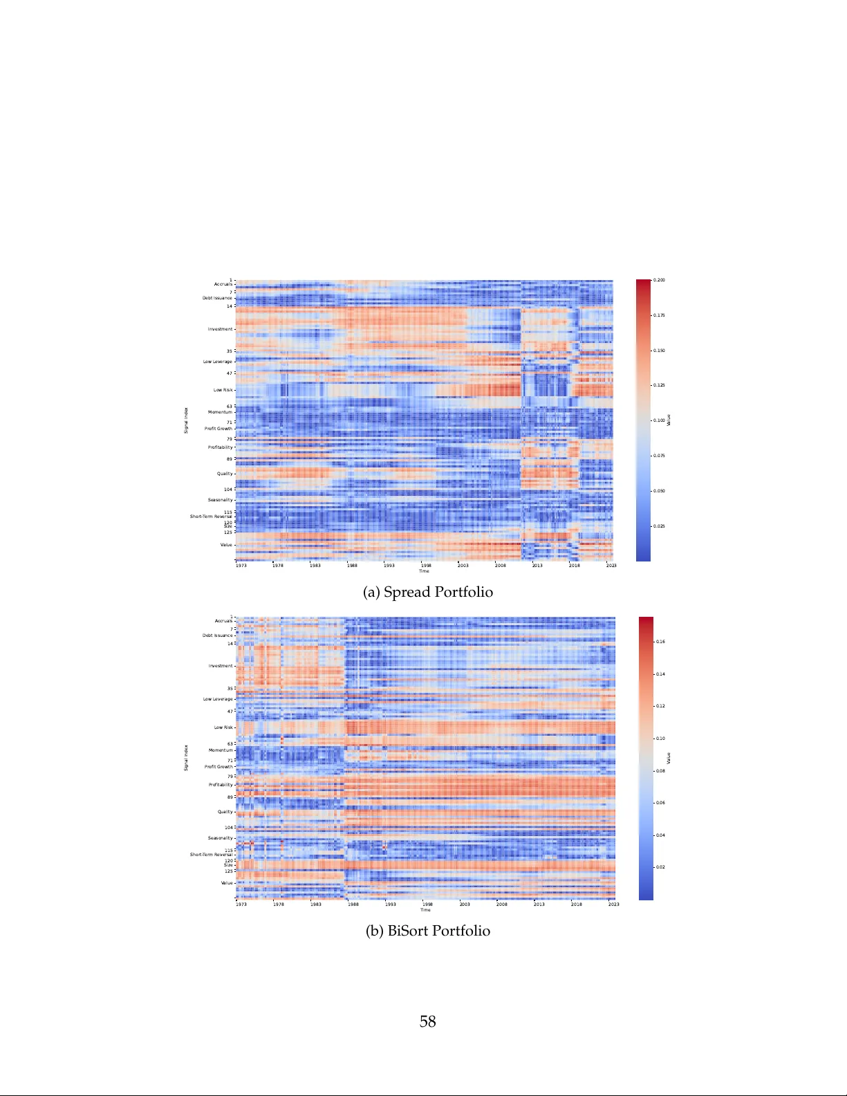
Stochastic Discount Factors with Cr oss-Asset Spillovers * Dor on A vramov Reichman University (IDC), Herzliya, Israel Xin He University of Science and T echnology of China February 25, 2026 Abstract This paper develops a uniﬁed framework that links ﬁrm-level predictive signals, cross-asset spillovers, and the stochastic discount factor (SDF). Signals and spillovers are jointly estimated by maximizing the Sharpe ratio, yielding an interpretable SDF that both ranks characteristic relevance and uncovers the direction of predictive in- ﬂuence acr oss assets. Out-of-sample, the SDF consistently outperforms self-predictive and expected-return benchmarks across investment universes and market states. The inferred information network highlights large, low-turnover ﬁrms as net transmitters. The framework offers a clear , economically grounded view of the informational archi- tecture underlying cr oss-sectional return dynamics. Key W ords: Asset Pricing, Connection Matrix, Cross-Asset Spillover , Sharpe Ratio, Stochastic Discount Factor . JEL classiﬁcation: C1, G11, G12. * W e are grateful to Utpal Bhattacharya, Lin W ill Cong, Y i Ding, Gavin Feng, Shuyi Ge, Michael Gofman, Jingyu He, Kewei Hou, W enjin Kang, Shikun Barry Ke, Junye Li, Sicong Li, Xin Liu, Semyon Malamud, Stefan Nagel, Zilong Niu, Alex Philipov , Gil Segal, Giorgia Simion, Robert Stambaugh, Y inan Su, Dragon Y ongjun T ang, Jun T u, Siwei W ang, Y anchu W ang, Dacheng Xiu, Jingzhou Y an, Jingyi Y ao, Jun Y u, Chao Zhang, Dake Zhang, Guofu Zhou, Qi Zhou, and seminar and conference participants at Hebrew University of Jerusalem, Shanghai Jiao T ong University , Sichuan University , Southwestern University of Finance and Economics, Uni- versity of Science and T echnology of China, Xiamen University , Fudan International Symposium on AI in Finance 2025, Hong Kong Confer ence for Fintech, AI, and Big Data in Business 2025, Paris December Finance Meeting 2025, SYSU Conference on Big Data, AI, and FinT ech 2025, UMacau FinT ech and Financial Markets W orkshop 2025, and USTC Frontiers in Finance Conference 2025, for constructive discussions and feedback. The authors acknowledge ﬁnancial support from Inquir e Europe. A vramov (E-mail: doron.avramov@runi.ac.il ) is at Reichman University (IDC), Herzliya, Israel. He (E-mail: xin.he@ustc.edu.cn ) is at University of Science and T echnology of China. All authors con- tributed equally to this work. 1 Introduction The central objective of empirical asset pricing is to identify ﬁrm-level signals that ex- plain the cross-section of expected stock returns—whether through exposure to risk factors or persistent mispricing. The dominant paradigm, gr ounded in the assumption of self- predictability , asserts that a ﬁrm’s own characteristics forecast its own returns (see, e.g., Cochrane ( 2011 ); Harvey et al. ( 2016 )). Complementing this view is a growing literature on cross-predictability—the idea that the characteristics or returns of one asset can help forecast the returns of others (see, e.g., Lo and MacKinlay ( 1990 ); Hou ( 2007 ); Cohen and Frazzini ( 2008 ); Cohen and Lou ( 2012 ); Huang et al. ( 2021 , 2022 )). A key mechanism un- derpinning this phenomenon is the presence of lead–lag effects, whereby price movements or information from one ﬁrm precede and predict those of related ﬁrms. Such ef fects can stem from staggered information diffusion, peer inﬂuence within industries, supply chain linkages, or correlated trading by institutional investors that induces price pressure acr oss related assets. Despite r ecent methodological advances in modeling cross-stock predictability , sev- eral foundational questions remain unresolved. Chief among them is how a mean–variance investor can analytically integrate multiple predictive signals when returns are intercon- nected across assets. Equally crucial is developing a framework that jointly captures both the relevance of individual signals and the structur e of return spillovers—enhancing port- folio performance while preserving interpr etability . This paper addresses these questions by proposing a uniﬁed and systematic frame- work for constructing maximum–Sharpe ratio strategies. W e combine ﬁrm-level signals through a ﬂexible weighting vector (the signal-aggregation vector Λ ) and model cross- asset spillovers using a structur ed connection matrix (the spillover matrix Ψ ). The resulting optimal strategy admits a transparent analytical characterization. This formulation natu- rally connects to the stochastic discount factor (SDF; see Hansen and Jagannathan ( 1991 ); Cochrane ( 2009 ); Back ( 2017 )), which, in this context, takes the form of a single factor that prices the cross-section of r eturns. An important distinction in the asset pricing literature lies between conditional and unconditional Sharpe ratio optimization. As emphasized by Hansen and Richard ( 1987 ), conditional optimization targets the best return–risk trade-off at each point in time us- ing the information then available, whereas unconditional optimization maximizes this trade-off in expectation using long-run moments. 1 Our framework follows the latter ap- 1 See also Lewellen and Nagel ( 2006 ), who emphasize the distinction between conditional and uncondi- tional beta pricing. 1 proach: while it incorporates time-varying signals—such as ﬁrm characteristics and cross- asset linkages—the stochastic discount factor is optimized to perform well on average over time. This orientation prioritizes long-horizon performance over period-by-period ef ﬁ- ciency , yielding strategies that are transparent, r obust, and empirically gr ounded. While the analytical formulation provides a population-level characterization of the Sharpe-optimal SDF , our empirical implementation uses a regression-based pr ocedur e tai- lored for high-dimensional applications. W e build on the approach of Britten-Jones ( 1999 ) and employ ridge-type regularization—with a single tuning parameter λ chosen by ﬁve- fold cross-validation—to estimate both the signal weights and the connection matrix. This method converges to the theoretical solution in large samples while enhancing numeri- cal stability and interpretability . Unlike expected return-maximization—which, under cer- tain speciﬁcations, can lead to extreme concentration in a single predictor—Sharpe ratio- maximization encourages diversiﬁcation acr oss signals, thereby enhancing r obustness and practical relevance. T o build intuition, we start with a low-dimensional toy example using ﬁve well-known ﬁrm characteristics and nine portfolios sorted by size and book-to-market. This simpliﬁed setting enables us to illustrate the estimated signal weights, cross-asset linkages, and result- ing trading strategy in full detail. W e evaluate performance with a rolling out-of-sample procedur e, re-estimating the strategy each month using the prior 10 years of data. Even in this controlled environment, the maximum–Sharpe ratio strategy based on cross-stock predictability attains an annualized Sharpe ratio of 1.22, compared with 0.60 for the self- predictive benchmark—an improvement driven simultaneously by cr oss-asset spillovers, shifts in signal relevance, and their interaction. W e then scale the framework to a compr ehensive empirical setting using 138 ﬁrm- level signals fr om the Jensen et al. ( 2023 ) dataset. Our primary investment universe con- sists of 138 univariate spread portfolios spanning 1963–2023. W e also consider a broader set of 544 bivariate portfolios sorted by ﬁrm size and a secondary characteristic. Apply- ing the same rolling 10-year estimation scheme, the maximum–Sharpe ratio (MS) strategy attains annualized Sharpe ratios of 2.21 and 3.32 on the spread and bi-sort portfolios, re- spectively—consistently outperforming both self-predictive benchmarks and maximum- expected return (MR) strategies. Speciﬁcally , the Sharpe ratio of our cr oss-predictive SDF strategy exceeds that of a self-predictive Sharpe ratio–maximizing benchmark by 0.79 on spread portfolios and more than 1.26 on bi-sorted portfolios—translating into economi- cally meaningful gains in certainty-equivalent returns. Mor eover , compar ed to expected return–maximizing strategies, our Sharpe ratio–maximizing SDF improves risk-adjusted performance by factors of 4–10, depending on the investment universe and market regime. 2 T o assess robustness, we evaluate performance across differ ent market environments. W e split the test sample by investor sentiment and by volatility regimes based on the VIX index. The Sharpe ratio–maximizing strategy maintains strong performance across all sub- samples. For example, in high-sentiment periods, the strategy delivers a Sharpe ratio of 2.19 on spread portfolios and 3.58 on bi-sort portfolios. Even in low-sentiment or high- volatility regimes—conditions that typically challenge individual anomaly-based strate- gies—the strategy sustains Sharpe ratios above 2. These results contrast with the mor e state-dependent performance of expected return–maximizing portfolios. The SDF deﬁnes a single factor that, ex ante, prices the cross-sectional variation in expected returns of the test assets. W e evaluate whether this factor ’s payoffs are priced by leading asset pricing models and ﬁnd sizable, statistically signiﬁcant alphas relative to a broad set of benchmarks. These include the liquidity factor Pastor and Stambaugh ( 2003 ), the Fama–French ﬁve-factor model Fama and French ( 2015 ), the q-factors Hou et al. ( 2015 ), the mispricing factors Stambaugh and Y uan ( 2017 ), the behavioral factors Daniel et al. ( 2020 ), and a comprehensive fourteen-factor model. Across all speciﬁcations, the strategy delivers alphas of about 0.25% per month with t -statistics above 11, indicating that the r eturn variation embedded in cr oss-asset spillovers is not captured by existing models. Upon optimizing the Sharpe ratio, we uncover the underlying economic drivers of return predictability . By examining the estimated weights assigned to ﬁrm-level charac- teristics, we ﬁnd that the most inﬂuential predictors cluster in the categories of invest- ment, value, and proﬁtability , with signals such as liquidity of book assets, dividend yield, and return on equity consistently receiving the highest weights. In contrast, r eturn-based signals—including momentum, short-term reversal, and seasonality—exhibit persistently low weights. This pattern suggests that the cross-predictive SDF is primarily anchor ed in stable ﬁrm fundamentals rather than transitory market signals. In optimizing the Sharpe ratio, we also obtain a connection matrix, denoted by Ψ , that encodes the predictive relationships acr oss stocks. Each entry Ψ i,j reﬂects the extent to which signals fr om asset i forecast the returns of asset j , while diagonal elements r epresent self-predictive str ength. Empirically , the average off-diagonal entry is substantial—often exceeding the average diagonal—indicating that cr oss-asset predictive linkages carry more information than self-predictive signals alone. Aggregating rows and columns of the ma- trix following Diebold and Yılmaz ( 2014 ), we uncover a directional structure: certain stocks consistently act as net transmitters of pr edictive signals, while others serve primarily as net receivers. T ransmitters ar e typically large and low-turnover , wher eas receivers tend to be smaller , high-turnover stocks with characteristics such as value orientation, high proﬁtabil- 3 ity , low investment activity , and strong past r eturns. It is worth noting that the Sharpe ratio of the cr oss-predictive strategy is time-varying and declines notably after 2000. In the 1990s, the strategy delivers exceptional performance, with Sharpe ratios exceeding 2 on spr ead portfolios and above 4 on bi-sort portfolios. How- ever , performance attenuates in the post-2000 period, mirr oring the broader decline in self- predictability . For instance, Green et al. ( 2017 ) document that many anomaly portfolios become less proﬁtable after 2003, attributing the decline to the widespread adoption of anomaly-based strategies, impr oved market liquidity , and the growth of passive ETF in- vesting. Despite this attenuation, the pr oposed strategy maintains strong performance fr om 2000 to 2023, achieving Sharpe ratios of 1.58 (spr ead portfolios) and 2.21 (bi-sort portfo- lios)—substantially higher than those of standard benchmark factors: 0.41 (market), 0.27 (size), 0.20 (value), 0.54 (proﬁtability), 0.43 (investment), and 0.09 (momentum). By the end of 2023, ﬁve-year trailing Sharpe ratios decline to approximately 1.2 for the spr ead and bi-sort strategies, yet both remain consistently superior to traditional benchmarks even in recent years. The paper proceeds as follows. Section 2 presents the econometric framework. Sec- tion 3 outlines the estimation methodology . Section 4 describes the data. Section 5 reports the empirical ﬁndings. Section 6 concludes. 2 Econometric Framework W e consider an investment universe consisting of N risky assets. At each time t , the investor observes a signal matrix S t ∈ R N × M , where each r ow corresponds to one asset and contains M predictive characteristics (e.g., size, valuation, pr oﬁtability , investment, past returns). Each column of S t is cross-sectionally standar dized to have zer o mean and unit variance. Although our framework allows for a time-varying number of assets, the empirical analysis focuses on a ﬁxed cross-section of sorted portfolios. W e deﬁne t = 1 as the ﬁrst period in which signals are observed, and t = T + 1 as the ﬁnal period in which asset returns ar e r ealized. 2.1 T rading Strategy A linear strategy that incorporates multiple signals and cross-predictability is speciﬁed as ω ′ t = Λ ′ S ′ t Ψ , (1) 4 where ω t ∈ R N denotes the portfolio weights, Λ ∈ R M assigns loadings to each signal, and Ψ ∈ R N × N encodes how signals from one asset inﬂuence positions across all assets. Speciﬁcally , the weight on asset i is determined by multiplying Λ ′ , S ′ t , and the i th column of Ψ , allowing all signals in S t to contribute to each asset’s position. The element Ψ i,j quantiﬁes the predictive impact of asset i ’s signals on asset j . Relative to Brandt et al. ( 2009 ), who model portfolio weights as a function of ﬁrm- speciﬁc attributes, our framework generalizes the approach by allowing economically mean- ingful cross-asset spillovers to shape portfolio allocations. Moreover , although we focus on linear strategies, the framework readily accommodates nonlinear extensions by enriching the signal matrix with polynomial or Fourier -based transformations. For instance, one can construct an expanded signal matrix of dimension N × M P , where the ﬁrst N × M block cor- responds to the original S t , the second to its elementwise squar e, and subsequent blocks to higher-or der transformations up to the P th power . Importantly , such extensions preserve the dimension of the Ψ matrix, while the Λ vector expands accordingly to accommodate the enlarged set of predictors—including higher-order powers of the original signals. W e leave the formal development and empirical implementation of such nonlinear extensions to future r esear ch. W e construct managed-portfolio returns in excess of the risk-free rate by interacting future r eturns with the curr ent values of predictive signals: Π s =  I N ⊗ r s  S t , (2) where Π s is an N 2 × M matrix of managed-portfolio returns, I N is the N × N identity matrix, r s is a vector of N excess returns realized at time s > t , and ⊗ denotes the Kronecker product. The expected returns on these managed-portfolios are then deﬁned as Π = E  Π s  . Additionally , deﬁne Φ = vec  Ψ ′  , (3) so that Φ ∈ R N 2 . The vectorized Φ and the matrix Π str eamline later expressions for port- folio outcomes. T o aid interpr etation, limit extr eme equity positions, and stabilize estimation, we im- pose Euclidean norm constraints on key parameters. Speciﬁcally , we set Λ ′ Λ = 1 , Φ ′ Φ = 1 , (4) where the Euclidean norm constraint on the vector Φ is equivalent to a Fr obenius norm 5 constraint on the matrix Ψ . From a Bayesian perspective, these constraints correspond to zero-mean Gaussian priors on Λ and Φ , inducing ridge-type regularization that penalizes large parameter values. Proposition 1 formulates the realized return of the strategy in a convenient form, along with the expected return and Sharpe ratio. Appendix A provides the pr oof. Proposition 1. The investment metrics are as follows: • The realized and expected r eturns can be expressed as π s = Λ ′ Π s Φ , (5) E ( π s ) = Λ ′ ΠΦ . (6) • The square of the Sharpe Ratio ( S R 2 ) is given by the following two equivalent expressions: S R 2 = Λ ′ A Φ Λ Λ ′ B Φ Λ , (7) S R 2 = Φ ′ A Λ Φ Φ ′ B Λ Φ . (8) Here, A Φ = Π ′ ΦΦ ′ Π , B Φ = (Φ ′ ⊗ I M )Σ Φ (Φ ⊗ I M ) , Σ Φ is the covariance matrix of vec (Π ′ s ) , and I M is the identity matrix of order M . Similarly , A Λ = ΠΛΛ ′ Π ′ , B Λ = (Λ ′ ⊗ I N 2 ) Σ Λ (Λ ⊗ I N 2 ) , Σ Λ is the covariance matrix of vec (Π s ) , and I N 2 is the identity matrix of order N 2 . W e offer several r emarks regar ding Proposition 1 . First, our empirical analysis primarily focuses on maximizing the Sharpe ratio, using expected return-maximization as a benchmark for comparison. While both objectives rely on the same expressions for expected returns, they lead to differ ent optimal estimates for the signal weight vector Λ and the vectorized connection matrix Ψ . In particular , expected return-maximization reduces to a bilinear optimization pr oblem with closed-form solu- tions, wher eas Sharpe ratio-maximization entails solving a generalized eigenvalue prob- lem via an iterative procedur e. Importantly , maximizing the squar ed Sharpe ratio necessitates the use of both repr e- sentations of the Sharpe ratio provided in Proposition 1 when estimating the optimal val- ues of Λ and Φ . Explicit solutions for both the expected r eturn and Sharpe ratio-maximization problems ar e pr esented later in the paper . Second, Pr oposition 1 makes extensive use of the vectorized form of Ψ , which fully retains the cr oss-predictive structur e embedded in Ψ . As a result, the information con- 6 tent relevant for cross-predictability is entirely preserved in Φ , ensuring that the resulting strategy remains gr ounded in the same underlying pr edictive relationships. Third, the expr ession for investment return offers an intuitive economic interpr etation of our trading strategy . Recall that Π denotes the matrix of managed-portfolio expected returns, with each of its N 2 rows repr esenting the expected value of one asset’s return multiplied by one of the M signals across the N assets. Under the normalization E [ S t ] = 0 , Π simpliﬁes to the covariance matrix between future asset r eturns and contemporaneous signal values. If characteristic m of stock j helps predict the future return of stock i , the corresponding element of Π will be nonzero, reﬂecting this pr edictability . Thus, in this framework, Λ assigns relative weights to signals, Φ encodes cross-asset interactions, and together they operate on the matrix Π to optimize investment metrics. Fourth, the expected return of the trading strategy can alternatively be expr essed as E ( π s ) = M X m =1 Λ m µ m , (9) where µ m = P N 2 p =1 Π pm Φ p repr esents a weighted combination of portfolio expected returns, with Π pm denoting the expected return of the corresponding managed-portfolio and Φ p capturing the strength of the p -th r elationship within the strategy . This expected-return expression is informative because it demonstrates that, whether subject to an L 1 constraint or left unconstrained, the optimal solution is a corner solution: the trading strategy is entirely driven by the predictor with the largest absolute value of µ m , denoted predictor j , with | Λ j | = 1 and all other elements of Λ equal to zero. In contrast, under an L 2 constraint, the optimal Λ (given Φ ) is proportional to the M -vector that collects the µ m values. By comparison, Sharpe ratio-maximization effectively harnesses the beneﬁts of diversiﬁcation across pr edictors, assigning meaningful weight to multiple signals. In the context of expected return-maximization, He et al. ( 2024 ) extend the principal portfolios framework of Kelly et al. ( 2023 ) from a single-signal to a multi-signal setting by introducing a three-dimensional pr ediction tensor . Our study should not be viewed as a multi-predictor extension of principal portfolios. Rather , we propose a framework that dif- fers in both econometric structure and economic objective. From a modeling standpoint, we focus on a two-dimensional matrix Π , where one dimension captures multiple signals and the other encodes cross-predictive relationships across assets. From an economic per- spective, the proposed methodology is explicitly designed to ﬂexibly optimize the Sharpe ratio. Fifth, the r ealized return π s of the maximum-Sharpe ratio portfolio is pr oportional to 7 the stochastic discount factor (SDF), as implied by the fundamental asset pricing identity ( Hansen and Jagannathan , 1991 ; Cochrane , 2009 ; Back , 2017 ): M s = 1 − ω ′ r s , with E [ M s r s ] = 0 , (10) where M s denotes the pricing kernel and ω is the vector of slope coefﬁcients. Identifying the true ω is challenging in ﬁnite samples due to the “limits to learning” highlighted by Didisheim et al. ( 2024 ). While the literature has proposed various estimators of the SDF , our appr oach intr oduces a novel proxy that explicitly captures cross-asset spillovers, dis- tinguishing it from prior work. Sixth, Kelly et al. ( 2023 ) focus on expected r eturn-maximization and propose an alpha- beta decomposition: the antisymmetric and symmetric components of the prediction ma- trix yield the principal alpha and principal exposure portfolios, r espectively . Although our expected return-maximizing strategy can be cast within this framework, our Sharpe ratio-maximizing strategy—by construction—excludes alpha, consistent with the SDF in- terpretation in Equation ( 10 ). Empirically , we demonstrate that expected return-maximizing and Sharpe ratio-maximizing strategies—both accounting for cr oss-asset spillovers—lead to substantially differ ent out- comes. The Sharpe ratio-maximizing strategy consistently delivers signiﬁcantly higher Sharpe ratios across the full sample, as well as during both expansion and contraction periods. Next, sorting assets by the estimated weights surfaces the portfolio’s informational backbone: it ranks assets by how much they raise the strategy’s risk-adjusted payof f. High- ranked (large-weight) assets ar e those that sharpen the payof f of the pricing kernel in three complementary ways: they carry economically meaningful fundamentals; they occupy ad- vantageous positions in the web of cr oss-asset co-movements that let the portfolio harness spillovers; and they help balance the residual risks created elsewhere in the strategy . An as- set can rank highly even if its own return is not strongly predictable—when it acts as a con- duit that improves how the portfolio captures cross-asset structur e or when it completes the diversiﬁcation needed to express valuable payoff dir ections more cleanly . Lower -ranked assets contribute less to efﬁciency either because their information is largely redundant or because they add volatility without commensurate beneﬁt. Finally , as shown in Appendix B , the connection matrix Ψ closely aligns with the pro- jection of stock returns onto the distinct elements of the signals. 8 2.2 Zero-Cost and Leverage Constraints Up to this point, we have only imposed norm constraints on the strategy’s positions. However , empirical asset pricing typically requir es a trading strategy , factor , or anomaly to take the form of a long-short portfolio—that is, to be zero-cost with total leverage equal to two. The following proposition imposes this zer o-cost constraint on the strategy . Proposition 2. A zero-cost trading strategy can be expr essed as follows: ω ′ t = Λ ′ S ′ t Ψ − 1 N Λ ′ S ′ t Ψ A, (11) = Λ ′ S ′ t ΨΘ , (12) where A is an N × N matrix, with each element set to one, and Θ = I N − 1 N A . Notice that ω ′ t ι N = 0 , wher e ι N is an N -vector of ones. Fortunately , all previous deriva- tions remain valid under the zer o-cost constraint. The necessary modiﬁcations are as follows. Deﬁne Π si = Θ( r s S ′ it ) for each i = 1 , 2 , . . . , N , and construct Π s by vertically stacking Π si . All investment metrics in Proposition 1 can then be re-derived under the zer o-cost constraint. In Appendix C , we demonstrate that the zero-cost constraint reduces the expected proﬁtability of the trading strategy . However , this constraint is essential for ensuring com- parability across strategies. In our empirical analyses, we primarily focus on zer o-cost strategies, wher e the long and short positions are of equal magnitude by construction. T o further ensur e comparabil- ity , we rescale these positions so that total portfolio leverage equals two. This adjustment aligns our strategies with standard practice in the literatur e (e.g., Fama and Fr ench , 1993 ). 3 Estimating the Unknown Parameters W e provide methods for estimating the unknown parameters underlying the trading strategy . 3.1 Maximizing Expected Return The following proposition pr esents the solution for the strategy that maximizes ex- pected return. 9 Proposition 3. By the Singular V alue Decomposition (SVD), Π can be decomposed as Π = U Λ Π V ′ , (13) where U is an N 2 × N 2 orthogonal matrix, Λ Π is an N 2 × M diagonal matrix of singular values, and V ′ is an M × M orthogonal matrix. The estimated parameters that maximize expected returns ar e given by ˆ Λ = V (: , 1) , (14) ˆ Φ = U (: , 1) . (15) These estimates correspond to the ﬁrst singular vectors from the matrices V and U , respectively . This choice ensures that the optimal trading strategy leverages the directions that capture the greatest variance in the pr ediction matrix Π , thereby extracting the most informative signal structure. Importantly , ˆ Λ and ˆ Φ are obtained from the singular value decomposition of the sample-based matrix Π , and should therefor e be interpreted as em- pirical estimators rather than population parameters. 3.2 Maximizing Sharpe Ratio The following pr opositions formulate the estimates that maximize the squared Sharpe ratio. Appendix D provides the pr oof and detailed derivations. Proposition 4. Assume that Φ is given. Based on ( 7 ) , deﬁne C Φ = B − 1 Φ A Φ . (16) The optimal Λ is the principal eigenvector Λ max of the eigenvalue problem C Φ Λ = λ Λ . (17) Similarly , assume Λ is given. Based on Equation ( 8 ) , deﬁne C Λ = B − 1 Λ A Λ . The optimal value for Φ is the largest eigenvector Φ max of the following eigenvalue problem: C Λ Φ = λ Φ . (18) The optimal solutions for Λ and Φ are obtained by iteratively applying these two equations until convergence. We further r escale each solution to have unit norm. 10 In this way , we utilize both alternative expressions for the Sharpe ratio in Proposition 1 to iteratively estimate the optimal parameters Λ and Φ . However , the eigenvalue pr ob- lems in ( 17 ) and ( 18 ) requir e computing the inverse of large matrices, which is challenging in high-dimensional settings. T o address this, we propose the following pr oposition to iteratively estimate Λ and Ψ . Proposition 5. Consider a set of managed-portfolios χ Φ of dimension T × M : χ Φ =       ( χ Φ ) ′ 2 ( χ Φ ) ′ 3 . . . ( χ Φ ) ′ T +1       , (19) where ( χ Φ ) s = Π ′ s Φ . (20) The pr oblem in ( 17 ) is essentially an asset-allocation exercise: it seeks to maximize the squar ed Sharpe ratio by investing in χ Φ composed of M assets. This is equivalent to estimating Λ as the mean-variance efﬁcient portfolio weights. Following Britten-Jones ( 1999 ), the estimate of Λ is obtained from the following regr ession: 1 = χ Φ Λ + u , (21) where 1 is a T -vector of ones and T denotes the sample size. T o handle high-dimensional settings, we adopt ridge regr ession ( Kelly and Xiu , 2023 ; Shen and Xiu , 2024 ). The estimator for Λ is then given by: ˆ Λ = ( χ ′ Φ χ Φ + λI M ) − 1 χ ′ Φ 1 , (22) where λ is a Ridge-type parameter that shrinks the regression coefﬁcients towards zer o. Similarly , we deﬁne a set of managed-portfolios χ Λ of dimension T × N 2 : χ Λ =       ( χ Λ ) ′ 2 ( χ Λ ) ′ 3 . . . ( χ Λ ) ′ T +1       , (23) where ( χ Λ ) s = Π s Λ . (24) 11 The problem in ( 18 ) is another asset allocation exercise: it seeks to maximize the squared Sharpe ratio by investing in χ Λ . The estimator for Φ is ˆ Φ = ( χ ′ Λ χ Λ + λI N 2 ) − 1 χ ′ Λ 1 . (25) W e highlight several key aspects of Sharpe ratio-maximization. First, the pr eceding propositions r ecast the problem as a managed-portfolio optimiza- tion, yielding the optimal weights for the tangency portfolio—or equivalently , for the stochas- tic discount factor (SDF). Second, we impose a common ridge penalty λ when estimating both Λ and Φ , thereby enforcing uniform shrinkage across all components. This shared r egularization parameter simpliﬁes exposition, enhances replicability , and mitigates overﬁtting in ﬁnite samples. W e implement the ﬁve-fold cross-validation scheme to select λ dynamically . Third, although the generalized eigenvalue solution pr ovides a population-level char- acterization of the Sharpe ratio-maximizer , in practice we replace the unknown moment matrices with their sample analogues and apply the same ridge penalty . Rather than solv- ing a generalized eigenvalue problem dir ectly , we cast the estimation as a single ridge- penalized regr ession. This approach recovers the optimal SDF direction in ﬁnite samples, improves numerical stability by shrinking weights on weak or collinear signals, and avoids the computational burden of eigendecomposition. The resulting weight vector exactly co- incides with the theoretical maximizer under the ridge-r egularized sample formulation. Fourth, the solution to the Sharpe ratio-maximizing strategy can be interpreted as a regularized linear combination of the principal components (PCs) of the matrix Π , with both Λ and Φ estimated via ridge regr essions on projected versions of Π . Unlike expected return-maximizing approaches that primarily load on the leading PCs, this strategy opti- mizes portfolio weights across the full spectrum of PCs. As a result, it captures predictive signals even in low-variance directions—consistent with the ﬁndings of Kelly et al. ( 2025 )— and achieves superior risk-adjusted performance. Fifth, our methodology for estimating the stochastic discount factor offers a distinct contribution to r ecent advances that emphasize ﬁrm characteristics (e.g., Kelly et al. ( 2019 ); Lettau and Pelger ( 2020 ); Chen et al. ( 2024 ); Feng et al. ( 2024 ); Didisheim et al. ( 2024 ); Cong et al. ( 2025 ); Liu et al. ( 2025 )). Unlike these approaches that treat assets independently , we incorporate structured cr oss-asset dependencies. This not only enhances empirical perfor- mance in out-of-sample tests but also yields a more interpretable economic narrative for how information propagates acr oss securities. Cross-asset dependencies are also central to recent transformer-based approaches in 12 asset pricing, which leverage multi-headed attention mechanisms to extract and aggregate predictive signals acr oss assets. For instance, Cong et al. ( 2022 ) intr oduce AlphaPortfolio, a deep reinforcement learning framework with cross-asset attention networks (CAAN) that model interdependencies among securities. Similarly , the AIPM framework of Kelly et al. ( 2024 ) embeds transformer architectur es within the SDF , showing that nonlinear informa- tion sharing across assets can signiﬁcantly impr ove empirical performance. While these transformer models offer substantial modeling ﬂexibility , our framework provides a complementary linear alternative that emphasizes transparency and interpretabil- ity . W e capture cross-asset spillovers through a connection matrix Ψ , where each element Ψ i,j quantiﬁes the predictive inﬂuence of asset i ’s signals on asset j ’s returns. Although related to the linear surrogate of the transformer , our approach dif fers in a key respect. The linear transformer models the attention matrix as a function of asset-level signals, requir - ing estimation of O ( M 3 ) parameters, wher e M denotes the number of characteristics. In such setups, signal r elevance and cr oss-asset dependencies ar e entangled within the signal space. By contrast, we disentangle these two components: signal relevance is captured by a vector Λ , while cross-asset connections are modeled separately via Ψ . This separation reduces parameter complexity to O ( M + N 2 ) , promotes computational ef ﬁciency , enables straightforward replication, and delivers an economically interpretable decomposition of predictive str ength and cr oss-asset signal spillovers. 4 Data Our dataset combines monthly stock returns from the Center for Research in Security Prices (CRSP), accounting variables from Compustat, and analyst coverage and earnings forecasts from the Institutional Br okers’ Estimate System (IBES). W e assume that quarterly and annual ﬁnancial statements from Compustat become publicly available four months after the end of the corr esponding ﬁscal quarter . The full sample spans January 1963 to De- cember 2023. Out-of-sample evaluation begins in February 1973, with estimation win dows based on rolling samples of the most r ecent 120 monthly observations. 4.1 Predictive Characteristics W e employ 138 ﬁrm-level signals across 13 characteristic themes: Accruals, Debt Is- suance, Investment, Leverage, Low Risk, Momentum, Proﬁt Gr owth, Pr oﬁtability , Quality , 13 Seasonality , Size, Short-T erm Reversal, and V alue. These signals originate from Jensen et al. ( 2023 ). 2 4.2 Spread Portfolios For each of the 138 signals, we sort stocks into ter ciles each month and compute high- minus-low factor returns. T o form factor-level signals, we aggregate stock-level signals into corresponding factor portfolios. Returns and signals are value-weighted by market equity , with individual market-equity weights winsorized at the 80th per centile of NYSE capitalization, following the data providers’ r ecommendations. 4.3 Bivariate Sorting on Size and Other Characteristics W e also construct bivariate sorted portfolios to serve as alternative investment uni- verse. First, stocks are sorted into two size gr oups (big vs. small) based on market equity . Independently , each signal sorts stocks into three groups (high, medium, low). Cr oss- classifying these sorts pr oduces six portfolios; we retain only the high and low portfolios for each size gr oup, resulting in four portfolios per signal. As with the spr ead portfo- lios, r eturns and signals ar e capped-value-weighted by winsorized market equity . W e om it the bivariate portfolios for the characteristic ami_126d due to missing r eturns in 2023. Moreover , since size already plays a role in the sorting procedur e, we consider a total of 136 × 4 = 544 portfolios. Thus, we consider two investment universes: one constructed from univariate sorts comprising 138 spread portfolios, and the other from bivariate sorts comprising 544 port- folios. Each portfolio is associated with a time series of returns and 138 signal observations. 2 W e use the “Global Stock Returns and Characteristics” dataset under “Contributed Data Forms” on WRDS: https://wrds- www.wharton.upenn.edu/pages/get- data/contributed- data- forms/ global- factor- data/ . T able IA.II of Jensen et al. ( 2023 ) details the signal deﬁnitions and refer ences. Of the original 153 signals, we exclude 15 that begin after 1963 to satisfy the sample-coverage requirements of Kelly et al. ( 2023 ). W e apply standard ﬁlters to retain only observations with: (i) excntry = “USA ”, (ii) CRSP shrcd ∈ { 10 , 11 } , (iii) CRSP exchcd ∈ { 1 , 2 , 3 } , and (iv) non-missing monthly excess return ( ret_exc ) and next-month excess return ( ret_exc_lead1m ). Each characteristic is standardized to have a mean of zero and a standard deviation of one. 14 5 Results 5.1 An Illustrative T oy Example T o build intuition for the proposed framework, we construct a low-dimensional toy dataset comprising ﬁve ﬁrm characteristics—market equity (ME), book-to-market ratio (BM), operating proﬁts to lagged book equity (OP), asset gr owth (INV), and 12-month mo- mentum (MOM)—and nine portfolios formed by a 3 × 3 sort on ME and BM (ranging from ME1×BM1 to ME3×BM3). This simpliﬁed setup allows us to explicitly report the estimated low-dimensional pa- rameters Λ and Ψ , as well as the weight vector ω . It also enables a comparison of key performance metrics for: (i) strategies subject to unit-norm constraints without an explicit zero-cost r equir ement; and (ii) zero-cost strategies with total leverage constrained to two. W e implement expected return and Sharpe ratio-maximizing strategies, as formulated in sections 2 and 3 . These strategies, which target differ ent objectives, yield notable differ- ences in parameter estimates and performance outcomes. T able 1 summarize the monthly average returns, monthly standard deviations, and annualized Sharpe ratios for each strat- egy over the out-of-sample period from Febr uary 1973 to December 2023. The ﬁrst two rows of the table consider the case in which the zero-cost assumption is not imposed. The r esults show that the strategy maximizing expected return (MR Cross) delivers a high average monthly r eturn of 5.56%, but with substantial volatility (standard deviation of 61.9%), yielding a Sharpe ratio of just 0.31. The Sharpe ratio-maximizing strategy (MS Cross) attains a mean return of 2.36% and a much lower volatility (9.78 %), yielding a Sharpe ratio of 0.84. Consequently , a mean– variance investor would ﬁnd the Sharpe ratio-maximizing strategy considerably more at- tractive, wher eas an investor solely targeting expected returns would prefer the expected return-maximizing strategy . Thus far , the out-of-sample performance aligns closely with the ex ante investment objectives. Next, we consider a strategy that maximizes the Sharpe ratio using self-prediction to isolate the incremental contribution of cr oss-predictive relations relative to self-predictive relations. The key distinction between these two strategies lies in the structure of the connection matrix Ψ . Under cross-pr ediction, Ψ is a full 9 × 9 matrix, capturing all pair- wise interactions among the characteristics and returns of assets. In contrast, under self- prediction, Ψ is restricted to its diagonal terms. The second and third rows of T able 1 report the performance of the Sharpe ratio–maximizing strategies under cr oss-prediction and self-prediction, respectively . The cross-pr ediction 15 strategy (MS Cross) delivers a Sharpe ratio of 0.84 with a mean return of 2.36%, whereas the self-prediction variant (MS Self) achieves a lower Sharpe ratio of 0.60 and the lowest mean return of 1.31% . This gap in both risk-adjusted and absolute returns illustrates the incremental beneﬁt of incorporating cross-pr edictive r elationships beyond self-prediction alone, underscoring the pivotal role of cr oss-predictive dynamics in enhancing portfolio performance. T o provide further economic perspective on the value of accounting for cross-stock predictability , we compute the certainty equivalent return of the investment strategies. The certainty equivalent is deﬁned as C E = µ − γ 2 σ 2 , where µ and σ ar e the expected return and volatility of the strategy , respectively , and the risk aversion parameter γ is set to 2. Accounting for cr oss-predictability , the certainty equivalent rate of r eturn is appr oximately 16.84% per year—8.00% higher than that of self-pr edictability—indicating economically signiﬁcant gains. W e next maximize expected return and Sharpe ratio under the zero-cost and leverage- two constraints. The fourth and ﬁfth rows of T able 1 report these constrained strategies, conﬁrming that imposing the zer o-cost r estriction reduces expected returns for both objec- tives. Nevertheless, even with zero cost and ﬁxed leverage, the Sharpe ratio–maximizing strategy outperforms the expected-r eturn–maximizing strategy , delivering a higher mean return (0.50% vs. 0.49%) and a substantially higher Sharpe ratio (1.22 vs. 0.53). T o provide additional insight into cross-pr ediction and self-prediction strategies, T a- ble 2 reports the estimated values of Λ , Ψ , and ω for each approach without imposing the zero-cost constraint. The estimation window spans 120 months, fr om December 2003 to November 2023, covering our last out-of-sample period. Panel A presents the Sharpe ratio-maximizing cross-pr ediction strategy; Panel B presents the Sharpe ratio-maximizing self-prediction strategy; and Panel C reports the differ ences in the portfolio weights ω be- tween the two. In T able 2 , Panel A shows that the estimated Λ coefﬁcient for book-to-market equity (BM) is − 0 . 34 , whereas the coefﬁcients for the other four characteristics are all positive, with the smallest value at 0 . 21 . This suggests that the Sharpe ratio–maximizing strategy with cross-pr ediction is well balanced across the ﬁve characteristics. The full 9 × 9 matrix Ψ exhibits substantial values both on and off the diagonal: the average absolute value of its diag onal entries is 0 . 0068 , compared to an average absolute off-diagonal entry of 0 . 0805 , indicating that cr oss-predictive relationships play an even more substantial role in deﬁning the trading strategy . Panel B of T able 2 shows that under self-prediction the estimated Λ coefﬁcients exhibit greater dispersion—asset gr owth (INV) even turns negative—while Ψ is constrained to its 16 diagonal (average absolute value of 0 . 0288 , all of f-diagonals zer o). This contrast highlights the structural ef fect of cross-predict ability: including cross-predictive terms not only yields nonzero off-diagonal elements of Ψ but also shifts the estimated Λ coef ﬁcients, altering the relative importance of characteristics. Panel C reports how the optimal weights ω shift between cross- and self-prediction: under cross-pr ediction, long exposures to ME3 BM1 decrease, and shorts in ME1 BM2 deepen. For example, the ME1 BM2 position is − 0 . 27 under cr oss-prediction—driven by off-diagonal Ψ entries of 0 . 24 and 0 . 25 —wher eas it is substantially smaller under self-prediction. As noted earlier , the optimal trading strategy that accounts for cross-pr edictability delivers a 8.00% higher certainty equivalent return, suggesting that the estimated Λ and Ψ , which determine the portfolio weights ω , differ to an economically signiﬁcant degree when cross-pr edictability is incorporated, r elative to the benchmark case of self-predictability . In summary , the results in T ables 1 and 2 conﬁrm that incorporating cross-pr edictive relationships is valuable for constructing robust investment strategies, even in a low-dimensional illustrative setting. T able 1: Performance of Strategies of a T oy Example This table reports the monthly average return (%), monthly standard deviation (%), and annualized Sharpe ratio for ﬁve strategies in a low-dimensional toy example involving ﬁve characteristics and nine assets. The strategies are: 1. Unconstrained expected return-maximization with cross-pr ediction; 2. Unconstrained Sharpe ratio-maximization with cross-prediction; 3. Unconstrained Sharpe ratio-maximization with self-prediction; 4. Zero-cost, leverage-two expected return-maximization with cr oss-prediction; 5. Zero-cost, leverage-two Sharpe ratio-maximization with cross-pr ediction. µ σ SR Cost MR Cross 5.56 61.9 0.31 Not Zero Cost MS Cross 2.36 9.78 0.84 Not Zero Cost MS Self 1.31 7.57 0.60 Not Zero Cost MR Cross ZC 0.49 3.22 0.53 Zero Cost MS Cross ZC 0.50 1.43 1.22 Zer o Cost 17 T able 2: Estimates for Λ and Ψ of a T oy Example This tables r eports the estimates for λ , Ψ , and ω of the Sharpe ratio-maximization strategies of the last rolling- window estimation, with cross-pr ediction in Panel A and self-prediction in Panel B. These strategies are fr ee from zer o-cost and leverage-two constraints. The Λ vector has ﬁve elements corr esponding to ﬁve character - istics: ME, BM, OP , INV , and MOM. There ar e nine assets for investment: the three-by-thr ee sorted portfolios on ME and BM. Speciﬁcally , they are ME1 BM1, ME1 BM2, ME1 BM3, ME2 BM1, ME2 BM2, ME2 BM3, ME3 BM1, ME3 BM2, ME3 BM3. The Ψ is a nine-by-nine matrix, where the element i,j corresponds to the strength of the predictive relationship of the asset i’s signals to asset j’s returns. For cross-prediction in Panel A, the Ψ has 81 values to estimate, while for self-prediction in Panel B, the Ψ is only active in 9 values in the diag- onal. In addition, the following two rows of panels A and B report the absolute average of the diagonal and off-diagonal terms of Ψ . Finally , Panel C shows the change of ω from cr oss- to self-prediction strategies. Panel A: Cross-Pr ediction Λ ME BM OP INV MOM 0.21 -0.34 0.29 0.53 0.69 Ψ 0.02 -0.05 0.01 -0.01 0.03 -0.03 -0.01 -0.04 0.02 0.03 -0.21 -0.05 0.06 0.16 -0.09 0.01 -0.06 0.15 0.03 0.24 -0.08 -0.02 -0.17 0.18 -0.04 0.09 -0.17 -0.12 0.15 0.06 0.02 0.12 -0.22 0.00 -0.03 0.07 0.09 -0.03 -0.09 -0.04 -0.01 0.04 0.02 0.10 -0.01 -0.03 -0.13 0.12 -0.05 -0.11 0.04 0.11 -0.07 0.07 0.13 -0.14 0.14 0.01 -0.26 0.23 0.08 0.00 -0.21 -0.14 0.25 -0.26 -0.05 0.13 0.00 -0.10 0.03 0.15 -0.02 -0.09 0.15 0.09 0.09 -0.14 -0.06 -0.02 -0.06 Absolute A verage of Diagonal T erms Ψ 0.0068 Absolute A verage of Off-Diagonal T erms Ψ 0.0805 ω -0.03 -0.27 0.20 0.00 -0.03 0.03 0.09 -0.06 -0.06 Panel B: Self-Prediction Λ ME BM OP INV MOM -0.09 -0.89 0.41 -0.14 0.12 Ψ -0.14 0 0 0 0 0 0 0 0 0 0.51 0 0 0 0 0 0 0 0 0 -0.13 0 0 0 0 0 0 0 0 0 -0.04 0 0 0 0 0 0 0 0 0 0.41 0 0 0 0 0 0 0 0 0 0.02 0 0 0 0 0 0 0 0 0 0.35 0 0 0 0 0 0 0 0 0 -0.63 0 0 0 0 0 0 0 0 0 -0.09 Absolute A verage of Diagonal T erms Ψ 0.0288 Absolute A verage of Off-Diagonal T erms Ψ 0 ω -0.14 -0.10 0.19 -0.03 0.00 -0.02 0.47 -0.32 0.08 Panel C: Change of W eights from Cross- to Self-Pr ediction ID ME1 BM1 ME1 BM2 ME1 BM3 ME2 BM1 ME2 BM2 ME2 BM3 ME3 BM1 ME3 BM2 ME3 BM3 0.10 -0.17 0.00 0.03 -0.03 0.05 -0.37 0.26 -0.13 18 T able 3: Performance of Cross-Pr edictive Strategies This table reports the monthly average return (%), monthly standard deviation (%), and annualized Sharpe ratio of cross-predictive strategies. The strategies are zero-cost and leverage two. MR and MS are strategies to maximize expected return and Sharpe ratio, respectively . Panels A and C are for investing in 138 spread portfolios, and Panels B and D are for 544 bivariate sorted portfolios. In Panels A and B, we report the r esults of the whole out-of-sample period from February 1973 to December 2023 and the high and low sentiment periods split by the sentiment median value over the sample periods from February 1973 to December 2023. In Panels C and D, we report for January 1990 to December 2023, and the high and low VIX periods split by the VIX median value over the sample periods from 1990 to 2023. 1973:02-2023:12 SENT High SENT Low µ σ SR µ σ SR µ σ SR Panel A: Spread Portfolios MR 0.42 3.23 0.45 0.73 3.79 0.67 0.11 2.53 0.15 MS 0.29 0.45 2.21 0.30 0.47 2.19 0.27 0.43 2.22 Panel B: BiSort Portfolios MR 0.45 3.02 0.52 0.48 3.35 0.49 0.42 2.66 0.54 MS 0.26 0.27 3.32 0.28 0.27 3.58 0.24 0.27 3.08 1990:01-2023:12 VIX High VIX Low µ σ SR µ σ SR µ σ SR Panel C: Spread Portfolios MR 0.33 3.83 0.30 0.59 4.97 0.41 0.07 2.14 0.12 MS 0.24 0.43 1.92 0.30 0.52 2.02 0.18 0.31 1.98 Panel D: BiSort Portfolios MR 0.39 3.20 0.42 0.57 3.87 0.51 0.20 2.33 0.30 MS 0.24 0.29 2.90 0.28 0.34 2.89 0.20 0.22 3.13 19 5.2 Zero-Cost Linear Strategies T able 3 reports the performance of linear cross-pr edictive strategies implemented as zero-cost, leverage-two portfolios, comparable to common factor and anomaly implemen- tations. MR and MS denote the strategies that maximize expected return and the Sharpe ratio, r espectively . In Panel A, we consider an investment universe with 138 spread port- folios detailed in the data section. Over the full sample period, MR achieves a monthly average r eturn of 0.42% with an annualized Sharpe ratio of 0.45, wher eas MS r ecords a lower monthly average return of 0.29% but a substantially higher annualized Sharpe ratio of 2.21. W e further analyze performance during evolving market states by splitting the out-of-sample period at the median of the investor sentiment index ( Baker and W urgler , 2006 ). 3 Dur- ing high-sentiment regimes, MR delivers an average monthly return of 0.73%, while in low-sentiment r egimes its r eturn falls to 0.11%. The MS strategy exhibits r obust Sharpe ra- tios across both regimes: 2.19 in high-sentiment periods and 2.22 in low-sentiment periods. In Panel B, we evaluate investments in 544 bi-variate sorted portfolios as detailed in the data section. Over the full out-of-sample period (January 1973–December 2023), MR delivers a monthly average return of 0.45% and an annualized Sharpe ratio of 0.52, whereas MS achieves an exceptionally high annualized Sharpe ratio of 3.32. In sub-period analyses, MR’s average r eturn incr eases during high-sentiment regimes, while MS maintains Sharpe ratios above 3 in both high- and low-sentiment periods. In Panels C and D, we split the period January 1990–December 2023 at the median of the VIX index. 4 In Panel C (spread portfolios), MR’s average return is 0.59% dur- ing high-VIX regimes and 0.07% during low-VIX regimes (0.33% full sample), while MS recor ds Sharpe ratios of 2.02 and 1.98 in high- and low-VIX r egimes (1.92 full sample). In Panel D (bi-variate sorted portfolios), MR attains a monthly average r eturn of 0.39% and an annualized Sharpe ratio of 0.42, while MS achieves a Sharpe ratio of 2.90. MR’s return r emains higher in high-VIX r egimes, and MS sustains Sharpe ratios around 3 in both high- and low-VIX regimes. In summary , MR strategies deliver high expected returns during high-sentiment and high-VIX r egimes, but considerably lower expected returns otherwise. In contrast, MS strategies consistently achieve superior Sharpe ratios across all market states. 3 The sentiment data spans July 1965 to December 2023 and is obtained from the variable ‘SENT” on Jeffrey W urgler ’s website: https://pages.stern.nyu.edu/~jwurgler/data/SENTIMENT.xlsx . 4 The VIX data spans 1990 to 2023 and is obtained from the CBOE: http://www.cboe.com/products/ vix- index- volatility/vix- options- and- futures/vix- index/vix- historical- data/ . 20 5.2.1 Comparing with Principal Portfolios (PP) W e compare the principal portfolio-based trading strategies of Kelly et al. ( 2023 ) with our own over the out-of-sample period from 1973 to 2019, as in their study . The r esults are reported in T able 4 . Panel A, row 1 (PP–ME), reports the performance of the ﬁrst principal portfolio on the market-equity signal: a 3.27% monthly expected r eturn, a 0.51 annualized Sharpe ratio, and a sum of absolute equity positions equal to 23.22. Rows 2 and 3 pr esent the ﬁrst princi- pal portfolios for the book-to-market and momentum signals, which achieve Sharpe ratios of 0.60 and 0.48, r espectively , with similarly high leverage. The principal portfolio can be applied to only one signal at a time. W e also consider to take the 1/N equal-weighted strat- egy of the ﬁrst principal portfolios acr oss all 138 signals, namely the PPEW strategy , which delivers a 2.83% monthly expected return and a 0.56 annualized Sharpe ratio. Notably , the leverage of PPEW is only 1.35, reﬂecting substantial diversiﬁcation beneﬁts by equal weighted average across pr edictors. Our maximum-expected return strategy achieves an 135.14% monthly expected re- turn and a 0.52 annualized Sharpe ratio, with leverage of 537.70. Overall, the maximum- expected return strategy slightly underperforms the principal portfolios in Sharpe ratio, albeit remains r easonably close to them. By contrast, the MS strategy harnesses multiple predictors to diversify exposures and optimize risk-adjusted r eturns, achieving an annualized Sharpe ratio of 2.22 with a lever - age factor of 438.01. While the principal portfolio appr oach tar gets expected r eturn subject to a volatility constraint, our strategy is derived dir ectly from Sharpe ratio-maximization. As a r esult, it places greater emphasis on balancing return and risk, leading to improved performance on risk-adjusted metrics in our empirical setting. T o enhance implementability , we impose zero-cost and leverage-two constraints on both strategies. Panel B of T able 4 reports the resulting performance. Under these con- straints, the maximum-expected-return strategy (Row 1) achieves a 0.46% monthly ex- pected return and an annualized Sharpe ratio of 0.51, while the maximum-Sharpe ratio strategy (Row 2) attains a 0.30% monthly expected return and an annualized Sharpe ratio of 2.33. In both cases, the portfolios maintain zero net cost and a constant leverage of two in every period. Overall, the maximum-Sharpe ratio strategy remains highly competitive—delivering superior risk-adjusted performance relative to a range of recent approaches, including principal portfolios. Accordingly , we focus our subsequent analyses to the constrained max-SR strategy . 21 T able 4: A First Comparison on the Performance of PP , MR, and MS This table reports each strategy’s monthly average return (%), monthly standard deviation (%), annualized Sharpe ratio, time-series average of the sum of positions on basic assets, and time-series average of the ab- solute sum of positions on basic assets. PP-ME is the Principal Portfolio strategy using the market-equity signal; PP-BM uses book-to-market; PP-MOM uses momentum. PP-EW is an equal-weighted combination of the ﬁrst principal portfolios of 138 signals. MR is our maximum-expected return strategy , and MS is our maximum-Sharpe ratio strategy . Panel A places no leverage or cost constraints on the strategies. Panel B imposes two constraints—a zero-cost requir ement and a leverage restriction—on all strategies. Data span January 1963 through December 2019 (from PP’s replication package on the Journal of Finance website), with the out-of-sample period running fr om February 1973 to December 2019. Strategy µ σ SR Sum ASum Panel A: Strategies PP-ME 3.27 22.32 0.51 23.21 23.22 PP-BM 4.64 26.94 0.60 12.62 14.45 PP-MOM 3.65 26.41 0.48 23.94 25.34 PPEW 2.83 17.52 0.56 1.03 1.35 MR 135.14 895.59 0.52 95.83 537.70 MS 68.65 107.15 2.22 48.33 438.01 Panel B: Strategies with Zero Cost MR 0.46 3.10 0.51 0.00 2.00 MS 0.30 0.45 2.33 0.00 2.00 22 T able 5: Cross- vs Self-Pr ediction This table reports the monthly average returns (%), monthly standard deviation(%), and annualized Sharpe ratio, time-series average of the sum of positions on basic assets, and time-series average of the absolute sum of positions on basic assets. The objective of the strategies is to maximize the Sharpe ratio. Notably , the cross-prediction strategies can be solved with and without the zero-cost constraint; however , the self- prediction strategy does not have an analytic solution once adding the zero-cost constraint. Panel A invests on spr ead portfolios and Panel B is for bivariate sorted portfolios. The out-of-sample period is Febr uary 1973 to December 2023. µ σ SR Sum ASum Panel A: Spread Portfolios MS Self 6.76 16.54 1.42 1.26 30.93 MS Cross 64.43 107.19 2.08 45.06 438.46 MS Cross ZC 0.29 0.45 2.21 0.00 2.00 Panel B: BiSort Portfolios MS Self 15.83 26.64 2.06 2.34 99.05 MS Cross 389.99 450.02 3.00 112.14 2154.07 MS Cross ZC 0.26 0.27 3.32 0.00 2.00 5.2.2 Cross-Prediction SDF versus Self-Prediction SDF The existing literature on SDF estimation has predominantly focused on self-pr edictive frameworks, where each asset’s signals are used solely to forecast its own returns. Kelly et al. ( 2019 ) pr opose Instrumented PCA with the belief that the factor loadings on SDF are determined by assets characteristics, overcoming the limitations of static loading in PCA. Lettau and Pelger ( 2020 ) ﬁnd that the SDF estimated on Risk-Premium PCA is more highly correlated with the true SDF than those estimated on PCA. Luo et al. ( 2025 ) esti- mate the SDF with observable characteristics-based factors with L1-penalized SDF regr es- sion; whereas, Didisheim et al. ( 2024 ) apply the L2-penalized SDF regr ession on observable and Random-Fourier -Feature generated factors. All of these papers have been working on high-dimensional characteristics-based portfolios to estimate the SDF , wher e the belief of self-prediction ar e embedded the portfolios. By contrast, our framework utilizes managed-portfolios inherently reﬂecting the belief 23 of cross-pr ediction: π s ( 6 ), χ Φ ( 19 ), and χ Λ ( 23 ). Whether cr oss-predictive strategies—where signals from one asset help predict the returns of others—can systematically outperform self-predictive ones in high-dimensional settings r emains an open question. T o investigate this, we construct the self-pr edictive strategy by restricting the matrix Ψ to its diagonal, thereby eliminating all cr oss-asset interactions. Panel A of T able 5 reports the empirical performance of the Sharpe ratio–maximizing strategies on the 138 spr ead portfolios. The self-pr edictive strategy achieves a Sharpe ratio of 1.42, while the cross-predictive counterparts attain Sharpe ratios of 2.08 without zero- cost requir ement and 2.21 with zero-cost and leverage-two constraints. This more than 0.60 differ ence in Sharpe ratio underscores the incremental value of incorporating cross-asset predictive signals. Panel B reports r esults for the 544 bivariate sorted portfolios. The self-predictive strat- egy achieves a Sharpe ratio of 2.06, while the cross-predictive variants reach 3.32 and 3.00 under constrained and unconstrained implementations, respectively . This gap of mor e than 1.00 in Sharpe ratio highlights the signiﬁcant contribution of off-diagonal elements in Ψ to improved portfolio performance. Overall, the evidence conﬁrms that cross-pr edictive strategies materially enhance the estimation and performance of stochastic discount factors—particularly in richer portfolio universes and longer samples. 5.2.3 Factor Spanning T ests W e conduct a series of factor-spanning tests to assess whether the established asset pricing factors fully explain the expected returns of the Sharpe ratio-maximizing strategies. T able 6 reports monthly alphas (%), factor loadings, and associated t -statistics. Panel A presents the Sharpe ratio-maximizing strategy on the spread portfolios, while Panel B r e- ports for the bivariate sorted portfolios. W e ﬁrst evaluate the Fama and Fr ench ( 2015 ) ﬁve-factor model (FF5). The strategy on spread portfolio exhibits modest loadings on Market ( β = − 0 . 01 , t = − 2 . 56 ) and SMB ( β = 0 . 01 , t = 1 . 78 ) but insigniﬁcant exposures to the other four factors, while delivering a highly signiﬁcant monthly alpha of 0.29% ( t = 13 . 29 ). This suggests that the strategy’s returns are largely orthogonal to the FF5 factors. Also, we augment the FF5 model with mo- mentum (UMD), short-term reversal (REV), and liquidity (LIQ) factors ( Pastor and Stam- baugh , 2003 ). In this expanded speciﬁcation, the strategy shows signiﬁcant loadings on UMD and REV but not on LIQ, while its alpha remains economically and statistically sig- niﬁcant at 0.26% ( t = 11 . 54 ). These ﬁndings indicate that momentum and reversal effects 24 partially explain the strategy’s performance, with little role for liquidity risk. Next, we then examine the Hou et al. ( 2015 ) four -factor model, which incorporates in- vestment (R_IA) and proﬁtability (R_ROE) factors alongside market and size factors. The strategy displays negligible loadings on R_IA and R_ROE, while maintaining a highly sig- niﬁcant alpha. The Stambaugh and Y uan ( 2017 ) mispricing factors—MGMT and PERF— also fail to subsume the strategy’s returns: The strategy shows minimal exposures to both factors, with an alpha of 0.28% ( t = 10 . 20 ). Then, we assess the Daniel et al. ( 2020 ) model, which includes the market factor and two behavioral factors, PEAD and FIN. While the strategy loads signiﬁcantly on PEAD, its alpha r emains robust at 0.29% ( t = 11 . 09 ), and it shows no meaningful exposure to FIN. Finally , in a comprehensive regr ession incorporat- ing all fourteen factors, The strategy maintains an alpha of 0.26% ( t = 8 . 04 ), with statisti- cally signiﬁcant but economically small loadings on SMB, UMD, REV , LIQ, FIN, and R_IA. These results collectively demonstrate that the strategy’s expected returns cannot be fully explained by existing factor models. Panel B corroborates these ﬁndings. The strategy on bivariate sorted portfolio displays statistically signiﬁcant but economically modest loadings on RMW , CMA, REV , PERF , R_IA, MGMT , and PERF . Notably , it maintains a monthly alpha of 0.25% ( t = 11 . 36 ) even after controlling for all fourteen factors, further supporting the strategy’s robustness to estab- lished factor models. Across all speciﬁcations—including the Fama–French ﬁve-factor model with UMD, REV , and LIQ augmentations, Hou–Xue–Zhang, Stambaugh–Y uan, and Daniel–Hirshleifer–Sun frameworks, and even the compr ehensive fourteen-factor regression—the Sharpe ratio- maximizing strategies on the spread and bivariate sorted portfolios exhibit persistently large and highly signiﬁcant alphas with only moderate loadings on existing factors. This suggests that conventional models may miss the cross-asset return pr edictability captured by our strategy . Below , we further analyze the pricing content of the Sharpe ratio-maximizing strategies. 25 T able 6: Alpha and Factor Loadings This table reports the monthly alphas (%), factor loadings, and their t -values (in parentheses) obtained from the factor-spanning tests of regressing the strategy returns on other asset pricing factors. W e have scaled the original strategy and factor returns by 100 for percentage compatibility , aiding coefﬁcient comparability . This table focus on the Sharpe ratio-maximizing strategies with zero cost and leverage two. Panel A displays the results for investing in spread portfolios, while Panel B shows for bivariate sorted portfolios. The factors include FF5 factor , momentum factor (UMD), short-term reversal factor (REV), liquidity factor (LIQ) from Pastor and Stambaugh ( 2003 ), short-horizon inattention factor (PEAD) and long-horizon ﬁnancing factor (FIN) fr om Daniel et al. ( 2020 ), investment factor (R_IA) and r eturn on equity factor (R_ROE) fr om Hou et al. ( 2015 ), management factor (MGMT) and performance factor (PERF) from Stambaugh and Y uan ( 2017 ). PEAD and FIN are available before December 2018. MGMT and PERF are available befor e December 2016. All other factors are available during the whole sample period. W e report with the Newey and W est ( 1987 ) t -statistics using a Bartlett kernel and lag length L = 4( T / 100) 2 / 9 . One, two, and three asterisks indicate signiﬁcance at the 10%, 5%, and 1% levels, respectively . Alpha Market SMB HML RMW CMA UMD REV LIQ PEAD FIN R_IA R_ROE MGMT PERF Panel A: Spread Portfolios 0.29*** -0.01** 0.01* -0.01 0.01 0.02 (13.29) (-2.56) (1.78) (-1.02) (0.98) (1.53) 0.26*** -0.01** 0.01 -0.00 0.01 0.01 0.03*** 0.02*** -0.00 (11.54) (-2.26) (1.48) (-0.16) (0.68) (0.91) (3.34) (2.74) (-0.82) 0.29*** -0.01 0.03** 0.01 (11.09) (-1.56) (2.14) (0.91) 0.28*** -0.01** 0.01* 0.01 0.01 (12.91) (-2.56) (1.95) (0.73) (1.24) 0.28*** -0.00 0.02** 0.02 0.03*** (10.20) (-0.47) (2.51) (1.19) (3.66) 0.26*** -0.01 0.01 -0.00 0.01 -0.03 0.01* 0.03*** -0.00 0.01 0.00 0.04 -0.05*** 0.01 0.04*** (8.04) (-0.92) (0.83) (-0.13) (0.44) (-0.72) (1.74) (3.05) (-0.51) (0.90) (0.37) (1.23) (-2.92) (0.51) (2.61) Panel B: BiSort Portfolios 0.25*** -0.00 0.01* -0.00 0.03*** 0.01 (16.67) (-0.62) (1.94) (-0.62) (3.96) (1.20) 0.24*** -0.00 0.01 0.00 0.02*** 0.01 0.02** 0.01 -0.00 (13.98) (-0.01) (1.59) (0.72) (3.92) (0.63) (2.21) (1.09) (-0.37) 0.25*** 0.00 0.02** 0.02*** (13.15) (1.23) (1.99) (2.70) 0.24*** -0.00 0.01** 0.01 0.02*** (14.61) (-0.53) (2.03) (1.23) (2.68) 0.26*** 0.01* 0.01 0.02*** 0.02*** (14.12) (1.81) (1.55) (3.02) (3.92) 0.25*** 0.01 0.01 0.00 0.02* -0.02 0.01 0.01 0.00 0.01 0.00 0.03 -0.02 0.01 0.02*** (11.36) (1.42) (1.58) (0.15) (1.88) (-0.96) (1.04) (1.51) (0.12) (1.38) (0.39) (1.11) (-1.29) (1.05) (2.69) 26 5.2.4 Evolution of Sharpe Ratios over the Sample Period T o assess the persistence and evolution of risk-adjusted r eturns over time, Figure 1 Panel A shows the ten-year trailing Sharpe ratios of our three maximum-Sharpe ratio strategies—MS Spr ead, MS BiSort and MS BiSort ﬁxed—alongside those of the market and momentum factors for comparison. 5 By smoothing over a decade window , we can observe how the trading strategies respond to changing market conditions. These strategies deliver eye-catching Sharpe ratios in the 1990s—MS BiSort climbs as high as 4–7 before 2000, and MS Spread approaches 4—reﬂecting their ability to capture persistent value-enhancing opportunities. After 2000, however , it is natural to see some attenuation: wider adoption of anomaly tradings, increased market liquidity , and a lower- volatility regime tend to compress excess returns over time. Accordingly , by the end of 2023, the trailing Sharpe of MS Spread and MS BiSort has moderated to about 1.2. By contrast, the MS BiSort ﬁxed seems to deliver even higher Sharpe ratios than MS BiSort, suggesting that our cross-validation scheme is conservative and provides a low bound for the out-of-sample performance. T o make more clear comparison, Figure 1 Panel B shows the Sharpe ratio of each strat- egy relative to that of MS BiSort ﬁxed. In early sample before 2000, the Sharpe ratio of MS Spread (MS BiSort) is approximately 60% (90%) that of MS BiSort ﬁxed, and market and momentum factors have below 20% Shape ratio relative to MS BiSort. In the most recent sample, the Sharpe ratios of MS Spread, MS BiSort, MKT -RF , and UMD are 70%, 75%, 43%, and 4% that of MS BiSort ﬁxed. For context, both the market factor ’s rolling Sharpe ratio and that of the momentum factor remain well below our strategies over the entire forty-year span. Although the per- formance gap narr ows in the post-2000 era, both maximum-Sharpe ratio strategies con- tinue to deliver robust risk-adjusted r eturns r elative to these benchmarks. T able 7 reports the (annualized) Sharpe ratios of the cross-predictive maximum-Sharpe ratio strategies, Fama-French ﬁve factors, and momentum factor for three sample periods: the whole OOS period fr om 1973:02 to 2023:12, before 2000:01, and after 2000:01. Although, the Sharpe ratios of our strategies attenuate after 2000, they remain competitive compared to the benchmark factors in three sample periods. 5 The shrinkage parameter λ for MS Spread and MS BiSort are selected via cross-validation. Appendix E reports the selected parameter values of time. MS BiSort ﬁxed uses a ﬁxed λ = 1 , which is the most frequently selected value. 27 Figure 1: Sharpe Ratio of Strategies The ﬁgure depicts ten-year trailing (annualized) Sharpe ratios for the cross-predictive maximum-Sharpe ratio strategies. “MS Spread” is the strategy to maximize Sharpe ratio investing in the spread portfolios.“MS BiSort” is the strategy to maximize Sharpe ratio investing in the bivariate sorted portfolios. “MS BiSort ﬁxed” uses a ﬁxed λ = 1 , which is the most frequently selected value. Panel A shows the Sharpe ratio, while Panel B shows the Sharpe ratio of each strategy divided by that of “MS BiSort.” The out-of-sample period is from February 1973 to December 2023 in monthly frequency , and the ﬁrst ten-year Sharpe ratio is obtained for January 1983. For comparison, the market factor (MKT -RF) and momentum factor (UMD) are included. 1990 2000 2010 2020 0 2 4 6 8 MS BiSort fix ed MS BiSort MS Spr ead MK T -RF UMD (a) Sharpe Ratio 1990 2000 2010 2020 0.0 0.2 0.4 0.6 0.8 1.0 (b) Sharpe Ratio Relative to MS BiSort 28 T able 7: Comparing Sharpe Ratios with Prevailing Factors The table reports the (annualized) Sharpe ratios of the cross-predictive strategies, Fama-French ﬁve factors, and momentum. Three sample periods ar e 1973:02 to 2023:12, 1973:02 to 1999:12, and 2000 to 2023. MS Spread MS BiSort MKT -RF SMB HML RMW CMA UMD 1973-2023 2.21 3.32 0.45 0.21 0.33 0.45 0.5 0.45 1973-1999 2.84 4.98 0.48 0.16 0.47 0.36 0.58 0.96 2000-2023 1.58 2.21 0.41 0.27 0.20 0.54 0.43 0.09 T able 8: T op T en Signals by Λ This table reports the top ten most important signals, Panel A for spread portfolios and Panel B for bivariate sorted portfolios. The columns are abbreviation, theme, time-series average of absolute Λ , full name, and original publication of the signals. There ar e 13 themes following Jensen et al. ( 2023 ). Abbreviation Theme Λ Full Name Publication Panel A: Spread Portfolio 2 aliq_at Investment 0.139 Liquidity of book assets Ortiz-Molina and Phillips ( 2014 ) 34 div12m_me V alue 0.126 Dividend yield Litzenberger and Ramaswamy ( 1979 ) 7 at_me V alue 0.125 Assets-to-market Eugene and French ( 1992 ) 9 be_gr1a Investment 0.125 Change in common equity Richardson et al. ( 2005 ) 44 emp_gr1 Investment 0.123 Hiring rate Belo et al. ( 2014 ) 45 eq_dur V alue 0.123 Equity duration Dechow et al. ( 2004 ) 24 col_gr1a Investment 0.123 Change in current ope. lia. Richar dson et al. ( 2005 ) 116 sale_gr3 Investment 0.123 Sales growth (3 years) Lakonishok et al. ( 1994 ) 15 bev_mev V alue 0.121 Book-to-market equity Penman et al. ( 2007 ) 10 be_me V alue 0.120 Book-to-market enterprise value Rosenberg et al. ( 1985 ) Panel B: BiSort Portfolio 71 ni_be Proﬁtability 0.141 Return on equity Haugen and Baker ( 1996 ) 86 ope_bel1 Proﬁtability 0.138 Ope. proﬁts-to-lagged be Fama and Fr ench ( 2015 ) 85 ope_be Proﬁtability 0.136 Operating proﬁts-to-be Fama and French ( 2015 ) 77 o_score Proﬁtability 0.135 Ohlson O-score Dichev ( 1998 ) 42 ebit_sale Proﬁtability 0.134 Proﬁt margin Soliman ( 2008 ) 90 prc Size 0.133 Price per share Miller and Scholes ( 1982 ) 41 ebit_bev Pr oﬁtability 0.132 Return on net operating assets Soliman ( 2008 ) 16 bidaskhl_21d Low Leverage 0.130 The high-low bid-ask spread Corwin and Schultz ( 2012 ) 65 mispricing_perf Quality 0.126 Performance Based Mispricing Stambaugh and Y uan ( 2017 ) 58 ivol_capm_252d Low Risk 0.126 Idio. vol. to CAPM (21 days) Ali et al. ( 2003 ) 29 5.3 Signal Importance T o understand the economic underpinnings of our Sharpe ratio-maximizing strategies or SDF , we examine the estimated values of Λ , which assign weights to ﬁrm-level predic- tive signals. These weights reﬂect the relative contribution of each signal to the SDF . W e focus on the absolute value of these weights averaged over time to assess long-term signal importance. T able 8 presents the ten most inﬂuential signals, ranked by their time-series average of absolute | Λ | values, where Panel A is for spread portfolios and Panel B is for bivariate sorted portfolios. Panel A, investing in spread portfolios, indicates that the most important signals ar e concentrated in the investment and value categories. For instance, the top signal— liquidity of book assets ( Ortiz-Molina and Phillips , 2014 )—receives an average importance of 0.139, while dividend yield ( Litzenberger and Ramaswamy , 1979 ), the leading signal in the value theme, ranks seventh overall with an importance of 0.126. These ﬁndings suggest that the strategy places greater emphasis on ﬁrm fundamentals linked to capital structur e, ﬁnanc- ing constraints, and valuation, rather than technical or return-based indicators. As for Panel B, proﬁtability dominates the top ten signals, followed by size , low leverage , and low risk themes. For instance, return on equity ( Haugen and Baker , 1996 ) and operating proﬁtability-to-lagged book equity ( Fama and French , 2015 ) are top signals, all belonging to proﬁtability . Besides, price per share ( Miller and Scholes , 1982 ) emerges from the size theme, recalling str onger size ef fects in the test assets sorted on size and other signals. Figure 2 presents the importance measures for all 138 signals, organized into 13 the- matic categories (as deﬁned in the Data section). Sub-ﬁgures (a) and (b) display theme- level importance for spread portfolios and bivariate-sorted portfolios, respectively . 6 The heatmap visualization employs color intensity to indicate importance levels—with red (blue) representing high (low) importance–allowing clear identiﬁcation of which signals consistently inﬂuence portfolio construction. In sub-ﬁgure (a) for spread portfolios, investment - and value -related signals dominate the r ed spectrum, reinfor cing the r ole of tangible ﬁrm fundamentals. In contrast, momen- tum , pr oﬁt growth , debt issuance , seasonality , and short-term reversal appear consistently in the blue range, indicating minimal weight in the Sharpe ratio-maximizing SDF . T urning to sub-ﬁgure (b) for bivariate-sorted portfolios, the proﬁtability theme dom- inates the heatmap, particularly following a pronounced r egime shift in the late 1980s. The size theme exhibits persistent importance thr oughout the sample period, r eﬂecting the strong cross-sectional dispersion in ﬁrm size within our test assets. In contrast, accruals , 6 W e provide the time-varying signal-level importance measur es in Figure F .1 of the Appendix F . 30 Figure 2: Signal Importance This ﬁgure depicts the heatmaps of signal importance Λ for each rolling-window estimation. Sub-ﬁgures (a) and (b) are for spr ead portfolios and bivariate sorted portfolios, respectively . For interpretation, we focus on the absolute value of elements in Λ . W e calculate the theme-level importance as the average of all signal-level importance within each theme. There ar e 13 themes following Jensen et al. ( 2023 ). 1973 1978 1983 1988 1993 1998 2003 2008 2013 2018 2023 T ime A ccruals Debt Issuance Investment L ow L everage L ow Risk Momentum P r ofit Gr owth P r ofitability Quality Seasonality Short T er m R eversal Size V alue Signal Theme Inde x 0.02 0.04 0.06 0.08 0.10 0.12 0.14 V alue (a) Spread Portfolio: Theme-Level 1973 1978 1983 1988 1993 1998 2003 2008 2013 2018 2023 T ime A ccruals Debt Issuance Investment L ow L everage L ow Risk Momentum P r ofit Gr owth P r ofitability Quality Seasonality Short T er m R eversal Size V alue Signal Theme Inde x 0.02 0.04 0.06 0.08 0.10 0.12 0.14 V alue (b) BiSort Portfolio: Theme-Level 31 proﬁt gr owth , seasonality , and short-term reversal show consistently low importance over the entire sample. Our analysis reveals that while the dominant predictive role of investment , value , prof- itability , and size themes remains stable over time, certain signals—particularly accruals and quality —exhibit heightened importance during high-volatility or low-sentiment peri- ods. This time variation suggests dynamic shifts in return predictability patterns, which our framework successfully captures thr ough its adaptive structur e. In summary , our signal importance analysis demonstrates that the cr oss-predictive SDF is primarily driven by stable, economically grounded predictors , with negligible depen- dence on transient or noisy effects. These ﬁndings not only underscore the robustness and economic interpretability of our framework but also open new avenues for investigating the fundamental drivers of cross-sectional r eturn pr edictability . 5.4 Networks in the Cross Section T o uncover the economic structure embedded in the cross-predictive matrix Ψ , we in- terpret Ψ as the adjacency matrix of a directed network acr oss N assets. This representation enables us to move beyond portfolio-level ef fects and examine how predictive information ﬂows through the cross-section. That is we identify assets that function as net transmit- ters or receivers of signals and assessing the alignment of these linkages with economic groupings such as ﬁrm size. Following the connectedness methodology of Diebold and Yılmaz ( 2014 ), we compute three metrics for each asset i — outgoing connectedness ( FROM ), incoming connectedness ( TO ) and net connectedness ( NET )—along with a market-level overall network intensity ( TOT AL ). Let Ψ i,j denote the pr edictive inﬂuence of asset i on asset j . W e deﬁne the network metrics as follows: FR OM i = N X j =1 j  = i | Ψ i,j | , (26) TO j = N X i =1 i  = j | Ψ i,j | , (27) NET k = TO k − FROM k , (28) TOT AL = 1 N N X i,j =1 i  = j | Ψ i,j | . (29) 32 Here, FR OM i measures the total str ength of predictive signals sent fr om asset i to others, capturing how much i contributes to forecasting the returns of other assets. TO j measures the total strength of predictive signals received by asset j from all other assets, reﬂecting how much j is inﬂuenced by the r est of the network. NET k is the differ ence between incoming and outgoing connectedness, indicating whether asset k is a net trans- mitter ( < 0 ) or net receiver ( > 0 ) of predictive information. TOT AL aggregates the overall off-diagonal magnitude of Ψ across all asset pairs, summarizing the average intensity of cross-asset pr edictive linkages in the network. The use of absolute values follows Diebold and Yılmaz ( 2014 ) and ensures all measur es are non-negative, thereby capturing signal strength r egar dless of sign. W e compute these metrics monthly for two asset universes—138 spread portfolios and 544 bivariate sorted portfolios—over T = 611 months. T o investigate the ﬁrm-level char- acteristics driving variation in connectedness, we estimate monthly cross-sectional regr es- sions: Connectedness i,t = α t + β ′ Char i,t + ε i,t , (30) where Connectedness i,t is one of FROM i , TO i , or NET i , and Char i,t is a vector of observ- able characteristics. W e r eport time-series averages of the estimated coef ﬁcients along with Newey–W est ( Newey and W est , 1987 ) t -statistics using a Bartlett kernel and lag length L = 4( T / 100) 2 / 9 ≈ 5 . T able 9 reports the r esults of monthly cr oss-sectional regr essions of thr ee network con- nectedness measures— FR OM , TO , and NET —on ﬁrm characteristics for two groups of test assets: spread portfolios (Panel A) and bivariate sorted portfolios (Panel B). The re- sults reveal economically intuitive patterns linking a stock’s network role to size, valuation, proﬁtability , investment, momentum, and several trading frictions. In Panel A for spr ead portfolios, the FR OM regr essions, measuring how much a stock helps predict others, we observe that smaller stocks (low ME), high book-to-market (BM), high proﬁtability (OP), and high momentum (MOM) stocks tend to transmit stronger sig- nals to others. These ﬁrms—small, value, proﬁtable, and past winners—have greater fore- casting inﬂuence, possibly because they aggregate market-wide information or drive co- movements. Additionally , stocks with low illiquidity (ILL) and low turnover (TRN) exhibit higher FROM, suggesting that liquidity increase a stock’s impact to the network. V olatil- ity (VL T), by contrast, enters positively , implying that more volatile stocks spill predictive attention. Notably , the coefﬁcient on size (ME) becomes insigniﬁcant, once contr olling ﬁve trading frictions, which means that the size effect on FROM is a manifestation of trading frictions but not size itself. 33 The TO regr essions, which capture how strongly a stock is predicted by others, show the opposite patterns on many characteristics. Stocks with high ME, high BM, low OP , low INV , high MOM, high VL T , and high BET A receive more pr edictive inputs fr om others. This suggests that ﬁrms that are large, volatile, illiquid, and priced as value stocks appear more susceptible to being forecasted using cross-asset information. Inter estingly , high- MOM stocks both receive and transmit signals, indicating they may act as informational ampliﬁers within the network. The NET r egressions, deﬁned as TO − FROM , consolidate these ef fects to identify whether a stock is a net receiver or transmitter of predictive information. Stocks that are large (high-ME), low-BM, low-OP , low-INV , and low-MOM tend to be net receivers, while small, value, proﬁtable, non-investing, and momentum-driven stocks are net transmitters. These directional patterns highlight a persistent asymmetry: small, value, strong proﬁtabil- ity , and conservative investment ﬁrms disseminate predictive signals, while lar ger and illiquid ﬁrms absorb them. In Panel B for bivariate sorted portfolio, these patterns still exist. For ease of interpre- tation, we focus on the NET r egressions. W e ﬁnd that small, low-BM, high-OP , low-INV , and low-MOM ﬁrms are net receivers in the network, while big, value, weak-proﬁtable, conservative-investing, and high-momentum stocks ar e net transmitters. After controlli ng ﬁve trading frictions in the regressions, the coefﬁcient on size become signiﬁcantly posi- tive, while other four coefﬁcients are unchanged. As for trading frictions, stocks with low volume, low volatility , high turnover , and low market-beta tend to receive spillovers from others than transmitting signals to others. T ogether , two sets of test assets demonstrate signiﬁcant correlations between network connectedness and asset characteristics, shedding light on that the determinants of cross- asset spillover effects. The estimated Ψ matrix embeds an economically interpretable hi- erarchy of signal ﬂows, shaped by ﬁrm fundamentals and market frictions. This struc- ture supports imposing sparsity or blockwise restrictions to enhance interpretability and control overﬁtting—especially by limiting signal ﬂows that contradict observed economic asymmetries. Nevertheless, the correlation between connectedness and asset character- istics depends on the choice of test assets. That is, differ ent test assets r eﬂect dif ferent patterns in asset pricing, see Feng et al. ( 2020 ); A vramov et al. ( 2025 ). In this speciﬁc exer- cise, we conﬁrm the prominent status of size as an asset characteristic in building sorted portfolios as test assets ( Fama and French , 1993 ). T able 9 connects to several literatur e. For bivariate portfolios (Panel B), we initially corroborate Lo and MacKinlay ( 1990 ), ﬁnding big stocks lead small stocks (coef ﬁcient - 0.15, row 1 on NET )—a r esult r obust to controlling for BM, OP , INV , and MOM (coef ﬁ- 34 cient -0.19, row 2). However , contr olling for trading frictions reverses the size coefﬁcient, suggesting big stocks become net receivers, warranting further investigation of size’s role in lead-lag effects. 7 Contrary to Chordia and Swaminathan ( 2000 ), we ﬁnd low-turnover stocks transmit signal to high-turnover stocks after controlling for size. 8 It holds for both spread and bivariate sorts. The divergence from prior papers reﬂects discretion in test as- sets and sample periods. Moreover , the two papers focus exclusively on weekly return spillovers, whereas we incorporate multiple ﬁrm-level monthly signals, including past re- turns. Collectively , we demonstrate that cross-asset spillovers ar e fundamentally linked to asset characteristics. Figure 3 depicts the TOT AL connectedness index—the average intensity of the of f- diagonal elements in Ψ —for both the 138 spread portfolios (dashed line) and the 544 bi-sort portfolios (solid line) ov er the 1973–2023 period. Four key ﬁndings emer ge. First, the time- series of TOT AL connectedness on the spread portfolios varies markedly through time: it troughs in the mid-1980s and again after 2020, but peaks around the early 1990s and during the post ﬁnancial crises, 2010s. Second, the indices for bivariate sorted portfolios share the trough in mid-1980s and peak in early 1990s, however , slight ﬂuctuations after 2000. Overall, the average level of TOT AL of spread portfolios is almost equal to that of bivariate sorted portfolios before 2000, but become higher after 2000. Thir d, despite these episodic surges, the time series reverts to a long-run mean near 0.72, suggesting a stable baseline level of cross-asset information transmission. T aken together , Figure 3 demonstrates that cross-asset spillover effects intensify dur - ing turbulent periods but persist as a pervasive market feature. These ﬁndings underscore the importance of modeling the full Ψ matrix—rather than restricting attention to its diag- onal elements—for constructing Sharpe ratio-maximizing portfolios. 7 For comparability , we replicate results for 1973-1987 (matching Lo and MacKinlay ( 1990 )’s sample end) and ﬁnd consistent size coefﬁcient signs. 8 While Chordia and Swaminathan ( 2000 ) uses "T rading V olume" in their title, they actually employ daily turnover as their volume proxy . 35 T able 9: Understanding Connectedness This table reports the time-series average and the Newey and W est ( 1987 ) t -statistics of cross-sectional re- gressions estimates for each month that regress a connectedness measure on asset characteristics. The assets are 138 spread portfolios in Panel A, and 544 bivariate sorted portfolios in Panel B. For ease of interpre- tation, the coefﬁcients are r eported with values multiplied by 1000. There are thr ee connectedness mea- sures: FROM , TO , and NET . The characteristics of interest are size (“market_equity”), book-to-market eq- uity (“be_me”), operating proﬁts-to-lagged book equity (“ope_bel1”), asset growth (“at_gr1”), price momen- tum t-12 to t-1 (“ret_12_1”), Amihud illiquidity(“ami_126d”), volume(“dolvol_126d”), volatility(“rvol_21d”), turnover(“turnover_126d”), CAPM beta (“beta_60m”), with abbreviations ME, BM, INV , OP , MOM, ILL, VLM, VL T , TRN, and BET A. There is an inter cept in the regression, but the estimates ar e omitted in the table. The sample period is from Febr uary 1973 to December 2023. ME BM OP INV MOM ILL VLM VL T TRN BET A Panel A: Spread Portfolio FROM -1.26 (-9.39) -2.62 7.78 4.75 0.80 4.83 (-7.62) (16.82) (8.39) (3.86) (20.28) 0.37 8.9 7.04 0.41 6.47 -7.49 -7.04 4.68 -2.49 -0.07 (0.16) (27.91) (14.08) (1.66) (21.42) (-1.35) (-1.5) (7.36) (-2.58) (-0.19) TO 0.72 (3.19) 1.65 0.90 -2.79 -1.66 2.63 (7.22) (3.27) (-7.43) (-9.71) (7.77) 17.47 2.84 -1.06 -1.77 4.03 -4.29 -15.46 5.55 -1.90 2.03 (8.3) (11.55) (-3.01) (-10.42) (9.79) (-1.11) (-3.55) (13.35) (-2.14) (5.38) NET 1.98 (6.45) 4.27 -6.88 -7.53 -2.46 -2.20 (9.78) (-14.07) (-11.09) (-11.32) (-6.05) 17.09 -6.06 -8.10 -2.19 -2.44 3.19 -8.42 0.86 0.58 2.11 (4.36) (-19.12) (-13.52) (-8.65) (-4.45) (0.49) (-1.42) (1.06) (0.38) (4.22) Panel B: BiSort Portfolio FROM 0.25 (12.53) 0.36 0.38 -0.30 0.59 0.52 (13.77) (16.23) (-16.54) (20.59) (20.31) 0.32 0.53 -0.16 0.69 0.73 1.39 2.22 0.56 -0.93 -0.03 (1.21) (18.89) (-6.22) (19.2) (15.16) (2.36) (2.98) (7.82) (-4.57) (-0.41) TO 0.10 (1.66) 0.17 -0.26 0.07 -0.33 -0.06 (2.86) (-4.79) (0.95) (-5.14) (-0.85) 3.82 -0.05 0.41 -0.45 -0.04 0.77 -3.96 -0.23 2.34 -0.50 (8.13) (-0.68) (5.21) (-6.84) (-0.54) (0.7) (-3.99) (-1.65) (10.22) (-3.7) NET -0.15 (-2.41) -0.19 -0.64 0.38 -0.92 -0.58 (-3.35) (-11.56) (4.54) (-11.36) (-10.22) 3.50 -0.59 0.58 -1.14 -0.77 -0.63 -6.18 -0.79 3.27 -0.47 (6.05) (-7.97) (6.49) (-13.19) (-10.66) (-0.63) (-5.47) (-5.92) (9.36) (-3.2) 36 Figure 3: T otal Connectedness This ﬁgure depicts the time-series plot of total connectedness of Ψ matrix over OOS period form February 1973 to December 2023. The blue dash line is for 138 spread portfolios, and the orange solid line is for 544 bivariate sorted portfolios. The shadow areas indicate for NBER r ecession periods. 1980 1990 2000 2010 2020 0.600 0.625 0.650 0.675 0.700 0.725 0.750 0.775 0.800 Spr ead BiSort R ecession T o analyze directional spillover effects in the bivariate-sorted portfolios mor e precisely , we decompose the Ψ matrix into four blocks (A, B, C, and D) according to ﬁrm size. Figure 4 presents the r esulting pr edictive information ﬂows across these partitions. Figure 5 presents the time series of absolute average values for each of the four blocks in Ψ . The r esults r eveal consistently stronger predictive relations in Block A (Small → Small) and Block C (Big → Small) compar ed to Block B (Small → Big) and Block D (Big → Big), particularly during the last two decades. The time-series averages ar e 1.50 and 1.53 for Blocks A and C, respectively , versus 1.09 and 1.11 for Blocks B and D. Notably , the divergence between the A/C and B/D blocks has incr eased substantially in r ecent years. These ﬁndings conﬁrm an asymmetric predictive structure, which aligns with the NET regr ession coefﬁcient of − 0 . 15 reported in Panel B of T able 9 . This result is consistent with the evidence in Lo and MacKinlay ( 1990 ), showing that lar ge stocks tend to lead small stocks, but not vice versa. The persistent and stable natur e of these patterns over time supports the economic rationale for imposing restrictions on Ψ , particularly by excluding 37 small-to-large pr edictive links. Furthermor e, the long-run regularity of these asymmetries suggests that dynamic sparsity str uctures—which adapt to time-varying network block strengths while maintaining economically motivated constraints—could of fer signiﬁcant modeling value. In summary , the connectedness analysis reveals that the connection matrix Ψ encodes economically meaningful structure. For bivariate sorted portfolios on size and other sig- nals, big stocks act as net transmitters of predictive signals; contr olling more signals, we ﬁnd that low trading volume, high turnover ratio, and low-beta stocks are net transmit- ters. Meanwhile, value, proﬁtable, non-investing, and high-momentum assets are mor e likely to be net receivers. The strength of cross-pr edictive relations is comparable to that of self-predictive effects. The overall network intensity ﬂuctuates over time, but remains around a stable level. Decomposing Ψ by ﬁrm size shows that predictive ﬂows from large to small ﬁrms dominate those in the reverse dir ection. Figure 4: Partition of Ψ in Size. This ﬁgure decomposes the Ψ matrix to four blocks based on ﬁrm size. They are: • A: Small (Stock Signals) → Small (Stock Returns), • B: Small → Big, • C: Big → Small, • D: Big → Big. A B C D Small Signal Big Signal Small Return Big Return 38 Figure 5: Absolute A verage of Four Blocks in Ψ : BiSort Portfolios This ﬁgur e shows the time-series plot of the absolute average of elements in four blocks of Ψ . The basic assets are the bivariate sorted portfolios, where four blocks A, B, C, and D repr esent the strength of cross- predictive relations for (1) small stock signals predict small stock returns, (2) small stock signals predict big stock returns, (3) big stock signals predict small stock returns, and (4) big stock signals predict big stock returns. The sample period is form February 1973 to December 2023. The shadow areas indicate for NBER recession periods. 1980 1990 2000 2010 2020 0.8 1.0 1.2 1.4 1.6 1.8 A B C D 39 6 Conclusion This paper develops a structured framework for constructing Sharpe ratio–maximizing investment strategies using multiple ﬁrm-level signals and accounting for informational linkages across assets. By jointly estimating signal relevance and a matrix capturing cr oss- asset pr edictive relationships, our approach yields closed-form portfolio weights derived from a generalized eigenvalue decomposition. In high-dimensional settings, estimation is implemented through Ridge-SDF regressions, which offer a stable and interpretable managed-portfolio repr esentation of the decision variables. The r esulting stochastic dis- count factor consistently delivers high out-of-sample Sharpe ratios across a range of asset universes and market conditions, outperforming both self-pr edictive models and expected return-maximization. Economically , the strategy is primarily driven by fundamental char- acteristics related to investment, valuation, and pr oﬁtability . In addition, the estimated connection matrix reveals that large and low-turnover stocks tend to act as net transmitters of pr edictive signals, while the overall strength of cr oss-asset linkages r emains persistently high over time. The paper opens several promising avenues for future research. First, the framework could be extended to other asset classes where cr oss-asset interdependencies ar e economi- cally meaningful, such as corporate bonds, curr encies, sover eign credit, or international eq- uities. For instance, in the corporate bond market, issuer fundamentals or equity-side infor- mation may predict bond returns through industry linkages, shared ownership networks, or common analyst coverage. Similarly , in curr ency markets, major r eserve curr encies may act as informational hubs whose movements help forecast subsequent shifts in peripheral currencies. Second, incorporating economic structur e into the modeling of cr oss-asset r ela- tionships could enhance both interpretability and predictive performance. As the number of assets and signals expands, estimating all possible interactions becomes incr easingly challenging. Imposing economically motivated constraints—such as directional spillovers based on ﬁrm size or sectoral hierarchies—could pr ovide a more structur ed and scalable approach. 40 References Ali, A., L.-S. Hwang, and M. A. T rombley (2003). Arbitrage risk and the book-to-market anomaly . Journal of Financial Economics 69 (2), 355–373. A vramov , D., G. Feng, J. He, and S. Xiao (2025). Schrödinger ’s sparsity in the cross section of stock returns. A vailable at SSRN: https://ssrn.com/abstract=5370960 . Back, K. (2017). Asset pricing and portfolio choice theory: 2nd edition . Oxford University Pr ess. Baker , M. and J. W urgler (2006). Investor sentiment and the cross-section of stock returns. Journal of Finance 61 (4), 1645–1680. Belo, F ., X. Lin, and S. Bazdresch (2014). Labor hiring, investment, and stock return pr e- dictability in the cross section. Journal of Political Economy 122 (1), 129–177. Brandt, M. W ., P . Santa-Clara, and R. V alkanov (2009). Parametric portfolio policies: Ex- ploiting characteristics in the cr oss-section of equity returns. Review of Financial Stud- ies 22 (9), 3411–3447. Britten-Jones, M. (1999). The sampling error in estimates of mean-variance ef ﬁcient portfo- lio weights. Journal of Finance 54 (2), 655–671. Chen, L., M. Pelger , and J. Zhu (2024). Deep learning in asset pricing. Management Sci- ence 70 (2), 714–750. Chordia, T . and B. Swaminathan (2000). T rading volume and cross-autocorr elations in stock returns. Journal of Finance 55 (2), 913–935. Cochrane, J. H. (2009). Asset pricing: Revised edition . Princeton university press. Cochrane, J. H. (2011). Presidential addr ess: Discount rates. Journal of Finance 66 (4), 1047– 1108. Cohen, L. and A. Frazzini (2008). Economic links and pr edictable returns. Journal of Fi- nance 63 (4), 1977–2011. Cohen, L. and D. Lou (2012). Complicated ﬁrms. Journal of Financial Economics 104 (2), 383–400. Cong, L. W ., G. Feng, J. He, and X. He (2025). Growing the ef ﬁcient fr ontier on panel trees. Journal of Financial Economics 167 , 104024. 41 Cong, L. W ., K. T ang, J. W ang, and Y . Zhang (2022). Alphaportfolio: Direct construction through deep reinfor cement learning and interpretable ai. A vailable at SSRN: https: //ssrn.com/abstract=3554486 . Corwin, S. A. and P . Schultz (2012). A simple way to estimate bid-ask spr eads from daily high and low prices. Journal of Finance 67 (2), 719–760. Daniel, K., D. Hirshleifer , and L. Sun (2020). Short- and long-horizon behavioral factors. Review of Financial Studies 33 (4), 1673–1736. Dechow , P . M., R. G. Sloan, and M. T . Soliman (2004). Implied equity duration: A new measure of equity risk. Review of Accounting Studies 9 , 197–228. Dichev , I. D. (1998). Is the risk of bankruptcy a systematic risk? Journal of Finance 53 (3), 1131–1147. Didisheim, A., S. B. Ke, B. T . Kelly , and S. Malamud (2024). Apt or “aipt”? the surpris- ing dominance of large factor models. NBER Working Paper: http://www.nber.org/ papers/33012 . Diebold, F . X. and K. Yılmaz (2014). On the network topology of variance decompositions: Measuring the connectedness of ﬁnancial ﬁrms. Journal of Econometrics 182 (1), 119–134. Eugene, F . and K. Fr ench (1992). The cross-section of expected stock returns. Journal of Finance 47 (2), 427–465. Fama, E. F . and K. R. Fr ench (1993). Common risk factors in the returns on stocks and bonds. Journal of Financial Economics 33 (1), 3–56. Fama, E. F . and K. R. French (2015). A ﬁve-factor asset pricing model. Journal of Financial Economics 116 (1), 1–22. Feng, G., S. Giglio, and D. Xiu (2020). T aming the factor zoo: A test of new factors. Journal of Finance 75 (3), 1327–1370. Feng, G., J. He, N. G. Polson, and J. Xu (2024). Deep learning in characteristics-sorted factor models. Journal of Financial and Quantitative Analysis 59 (7), 3001–3036. Green, J., J. R. Hand, and X. F . Zhang (2017). The characteristics that provide independent information about average us monthly stock returns. Review of Financial Studies 30 (12), 4389–4436. 42 Hansen, L. P . and R. Jagannathan (1991). Implications of security market data for models of dynamic economies. Journal of Political Economy 99 (2), 225–262. Hansen, L. P . and S. F . Richard (1987). The role of conditioning information in deducing testable restrictions implied by dynamic asset pricing models. Econometrica , 587–613. Harvey , C. R., Y . Liu, and H. Zhu (2016). . . . and the cross-section of expected returns. Review of Financial Studies 29 (1), 5–68. Haugen, R. A. and N. L. Baker (1996). Commonality in the determinants of expected stock returns. Journal of Financial Economics 41 (3), 401–439. He, S., M. Y uan, and G. Zhou (2024). Principal portfolios: The multi-signal case. A vailable at SSRN: https://ssrn.com/abstract=4245333 . Hou, K. (2007). Industry information diffusion and the lead-lag effect in stock r eturns. Review of Financial Studies 20 (4), 1113–1138. Hou, K., C. Xue, and L. Zhang (2015). Digesting anomalies: An investment appr oach. Review of Financial Studies 28 (3), 650–705. Huang, S., C. M. Lee, Y . Song, and H. Xiang (2022). A fr og in every pan: Information discreteness and the lead-lag returns puzzle. Journal of Financial Economics 145 (2), 83– 102. Huang, S., T .-C. Lin, and H. Xiang (2021). Psychological barrier and cross-ﬁrm r eturn predictability . Journal of Financial Economics 142 (1), 338–356. Jensen, T . I., B. Kelly , and L. H. Pedersen (2023). Is there a r eplication crisis in ﬁnance? Journal of Finance 78 (5), 2465–2518. Kelly , B., B. Kuznetsov , S. Malamud, and T . A. Xu (2024). Artiﬁcial intelligence asset pricing models. NBER W orking Paper: http://www.nber.org/papers/33351 . Kelly , B., S. Malamud, and L. H. Pedersen (2023). Principal portfolios. Journal of Fi- nance 78 (1), 347–387. Kelly , B. and D. Xiu (2023). Financial machine learning. Foundations and T rends® in Fi- nance 13 (3-4), 205–363. Kelly , B. T ., S. Malamud, M. Pourmohammadi, and F . T rojani (2025). Universal portfolio shrinkage. NBER W orking Paper: http://www.nber.org/papers/w32004 . 43 Kelly , B. T ., S. Pruitt, and Y . Su (2019). Characteristics are covariances: A uniﬁed model of risk and return. Journal of Financial Economics 134 (3), 501–524. Lakonishok, J., A. Shleifer , and R. W . V ishny (1994). Contrarian investment, extrapolation, and risk. Journal of Finance 49 (5), 1541–1578. Lettau, M. and M. Pelger (2020). Factors that ﬁt the time series and cross-section of stock returns. Review of Financial Studies 33 (5), 2274–2325. Lewellen, J. and S. Nagel (2006). The conditional capm does not explain asset-pricing anomalies. Journal of Financial Economics 82 (2), 289–314. Litzenberger , R. H. and K. Ramaswamy (1979). The ef fect of personal taxes and dividends on capital asset prices: Theory and empirical evidence. Journal of Financial Economics 7 (2), 163–195. Liu, Y ., G. Zhou, and Y . Zhu (2025). Maximizing the sharpe ratio: A genetic programming approach. A vailable at SSRN: https://ssrn.com/abstract=3726609 . Lo, A. W . and A. C. MacKinlay (1990). When are contrarian proﬁts due to stock market overreaction? Review of Financial Studies 3 (2), 175–205. Luo, B., G. Zhou, and T . Zhou (2025). Pricing kernel in high dimension: Factor selection, publication bias and relation to corporate bonds. Available at SSRN: https:// ssrn. com/abstract=5030128 . Miller , M. H. and M. S. Scholes (1982). Dividends and taxes: Some empirical evidence. Journal of Political Economy 90 (6), 1118–1141. Newey , W . K. and K. D. W est (1987). A simple, positive semi-deﬁnite, heteroskedasticity and autocorrelation consistent covariance matrix. Econometrica 55 (3), 703–708. Ortiz-Molina, H. and G. M. Phillips (2014). Real asset illiquidity and the cost of capital. Journal of Financial and Quantitative Analysis 49 (1), 1–32. Pastor , L. and R. F . Stambaugh (2003). Liquidity risk and expected stock returns. Journal of Political Economy 111 (3), 642–685. Penman, S. H., S. A. Richar dson, and I. T una (2007). The book-to-price effect in stock returns: Accounting for leverage. Journal of Accounting Research 45 (2), 427–467. 44 Richardson, S. A., R. G. Sloan, M. T . Soliman, and I. T una (2005). Accrual reliability , earn- ings persistence and stock prices. Journal of Accounting and Economics 39 (3), 437–485. Rosenberg, B., K. Reid, and R. Lanstein (1985). Persuasive evidence of market inefﬁciency . The Journal of Portfolio Management 11 (3), 9–17. Shen, Z. and D. Xiu (2024). Can machines learn weak signals? NBER Working Paper: http://www.nber.org/papers/w33421 . Soliman, M. T . (2008). The use of dupont analysis by market participants. The Accounting Review 83 (3), 823–853. Stambaugh, R. F . and Y . Y uan (2017). Mispricing factors. Review of Financial Studies 30 (4), 1270–1315. 45 Appendices A Proof of Proposition 1 Expected Return W e ﬁrst express π s , the realized return on the trading strategy , as a func- tion of the model parameters. Recognize that π s = Λ ′ S ′ t Ψ r s = P N i =1 Ψ ′ i r s S ′ it Λ = tr h Λ P N i =1 Ψ ′ i Π si i = Λ ′ Π ′ s Φ , wher e Ψ ′ i is a 1 × N vector which is the i -th row of Ψ , S ′ it is a 1 × M vector , which is the i -th row of S t , tr stands for the trace operator , and Π s is an N 2 × M matrix that vertically stacks the N × M matrices Π si = r s S ′ it for i = 1 , 2 , · · · , N . Then, on the basis of realized r eturn, the expected value is given by E ( π s ) = Λ ′ Π ′ Φ = Φ ′ ΠΛ . (A.1) V ariance Let Σ Φ be the covariance matrix of vec (Π ′ s ) . W e express π s in terms of vec (Π ′ s ) : π s = Λ ′ Π ′ s Φ = Λ ′ vec (Π ′ s Φ) . (A.2) Using the property of vectorization vec ( AB C ) = ( C ′ ⊗ A ) vec ( B ) , we get: vec (Π ′ s Φ) = (Φ ′ ⊗ I M ) vec (Π ′ s ) . (A.3) Therefor e: π s = Λ ′ (Φ ′ ⊗ I M ) vec (Π ′ s ) . (A.4) The variance of π s is: V ar ( π s ) = Λ ′ (Φ ′ ⊗ I M )Σ Φ (Φ ⊗ I M )Λ , = Λ ′ B Φ Λ , (A.5) 46 where B Φ = (Φ ′ ⊗ I M )Σ Φ (Φ ⊗ I M ) . W e consider an alternative expression of V ar ( π s ) . Let Σ Λ be the covariance matrix of vec (Π s ) . W e express π s in terms of vec (Π s ) : π s = Φ ′ Π s Λ = Φ ′ vec (Π s Λ) . (A.6) Again using the property of vectorization, we get: vec (Π s Λ) = (Λ ′ ⊗ I N 2 ) vec (Π s ) . (A.7) Therefor e: π s = Φ ′ (Λ ′ ⊗ I N 2 ) vec (Π s ) . (A.8) The variance of π s is: V ar ( π s ) = Φ ′ (Λ ′ ⊗ I N 2 )Σ Λ (Λ ⊗ I N 2 )Φ , = Φ ′ B Λ Φ , (A.9) where B Λ = (Λ ′ ⊗ I N 2 )Σ Λ (Λ ⊗ I N 2 ) . Sharpe Ratio W ith the expected return and variance, we express the Sharpe ratio square as: S R 2 = Λ ′ A Φ Λ Λ ′ B Φ Λ , (A.10) where A Φ = Π ′ ΦΦ ′ Π , B Φ = (Φ ′ ⊗ I M ) Σ Φ (Φ ⊗ I M ) , and Σ Φ is the covariance matrix of vec (Π ′ s ) . Alternatively , we express the Sharpe ratio squared as: S R 2 = Φ ′ A Λ Φ Φ ′ B Λ Φ , (A.11) 47 where A Λ = ΠΛΛ ′ Π ′ , B Λ = (Λ ′ ⊗ I N 2 ) Σ Λ (Λ ⊗ I N 2 ) , and Σ Λ is the covariance matrix of vec (Π s ) . These alternative expressions of S R 2 assist in ﬁnding the solution to maximize the Sharpe ratio. B Relating Φ to B When M = 1 Setup. Consider the return-generating pr ocess: r s = B S t + ε s , (B.1) where: • S t ∈ R N × 1 is the signal vector , • B ∈ R N × N is the slope matrix, • ε s ∼ (0 , Σ ε ) is a zero-mean innovation, • Σ S = E [ S t S ′ t ] is the signal covariance matrix. Managed-Portfolio Return. The managed-portfolio return vector is deﬁned as: Π s = ( I N ⊗ r s ) S t . (B.2) T aking expectations: Π = E [Π s ] = vec ( E [ r s S ′ t ]) = vec ( B Σ S ) . (B.3) In the case of a single signal, both Π and Π s are vectors of dimension N 2 , and Σ Λ denotes the covariance matrix of Π s . 48 Sharpe Ratio Maximization. W e maximize the Sharpe ratio subject to ∥ Φ ∥ = 1 : max Φ: ∥ Φ ∥ =1 Φ ′ Π √ Φ ′ Σ Λ Φ . (B.4) The optimal solution is: Φ = Σ − 1 Λ vec ( B Σ S ) ∥ Σ − 1 Λ vec ( B Σ S ) ∥ . (B.5) Thus, we obtain: B = unvec (Σ Λ Φ) · Σ − 1 S , (B.6) where un vec denotes the reshaping of an N 2 -vector into an N × N matrix. Expected Return Maximization. W e now maximize expected return subject to ∥ Φ ∥ = 1 : max Φ: ∥ Φ ∥ =1 Φ ′ vec ( B Σ S ) (B.7) The solution is: Φ = vec ( B Σ S ) ∥ vec ( B Σ S ) ∥ . (B.8) Inverting gives: B = unvec (Φ) · Σ − 1 S . (B.9) Intuition: Why Are the B Matrices Dif ferent? The differ ence stems from the objective: • Maximizing Expected Return: aligns Φ with the direction of highest expected payoff, ignoring variance. • Maximizing Sharpe Ratio: adjusts for risk by incorporating Σ Λ , penalizing high- volatility directions. 49 C Proof of Expected Return Reduction due to Zero-Cost Con- straint Consider the matrix Π formed by vertically stacking N matrices Π i , each of dimension N × M , and let ˜ Π be the matrix obtained after pre-multiplying each Π i by the matrix Θ , where Θ = I N − 1 N ι N ι ′ N . Here, Θ is a projection matrix that projects vectors onto the space orthogonal to the vector ι N of ones. Properties of Θ : • Θ is symmetric and idempotent, i.e., Θ 2 = Θ and Θ ′ = Θ , conﬁrming that it is a projection matrix. • The eigenvalues of Θ are 0 along the direction of ι N and 1 along all dir ections orthog- onal to ι N . Impact on Singular V alues: 1. The matrix Θ modiﬁes Π i by removing its component in the direction of ι N . This operation reduces the variance in Π i that is aligned with ι N . 2. Given the singular value decomposition of Π = U Σ V ′ , the transformation ˜ Π = (ΘΠ i ) can be viewed through the lens of modiﬁed singular vectors. Since Θ acts as an iden- tity on the space orthogonal to ι N and zeroes out components along ι N , it does not increase the magnitude of any singular vector components. 3. The singular values λ i ( ˜ Π) of the transformed matrix ˜ Π correspond to the norms of the vectors Θ U i , wher e U i are the left singular vectors of Π . Since Θ is a pr ojection (and thus a norm-reducing operation except wher e it acts as the identity), we have: ∥ Θ U i ∥ ≤ ∥ U i ∥ . (C.1) 50 4. Therefor e, the singular values of ˜ Π must satisfy: λ i ( ˜ Π) ≤ λ i (Π) . (C.2) for each i , because the projection does not increase vector norms and reduces them for vectors with non-zero components in the dir ection of ι N . T o be mor e pr ecise, the highest singular value of the transformed matrix does not change due to the preservation of the highest singular value by Θ . However , the transfor- mation induced by Θ results in a reduction of singular values in the transformed matrix ˜ Π in the other singular values, leading to a decrease in variance explained by certain com- ponents. Speciﬁcally , at least one singular value of ˜ Π is str ongly diminished compared to the corresponding singular value of the original matrix Π . This reduction underscores the effectiveness of the transformation in diminishing the inﬂuence of certain components in Π and highlights its r ole in variance r eduction. Hence, both expected r eturn and risk of the trading strategy are lower in the pr esence of the zer o-cost restriction. D Proof and Derivations for Propositions 4 and 5 This section focuses on maximizing the squared Sharpe ratio of a linear strategy . The results extend naturally to the Sharpe ratio maximization of a nonlinear strategy with an augmented signal space, for which we leave for future r esear ch. Maximizing the squar ed Sharpe ratio constitutes a generalized Rayleigh quotient problem , which can be solved via an eigenvalue problem . However , in empirical settings, the solution to this eigenvalue problem often becomes ill-conditioned in high-dimensional settings. T o address this issue, we employ Ridge-SDF regr essions to estimate the decision vari- ables, providing an intuitive managed-portfolio interpretation. Finally , we present an iter- ative algorithm to estimate Λ and Φ until conver gence. The details are as follows. 51 Deﬁne the squared Sharpe ratio as a function of Λ . According to Proposition 1 , the squared Sharpe ratio takes the form: S R 2 = Λ ′ A Φ Λ Λ ′ B Φ Λ , (D.1) where A Φ = Π ′ ΦΦ ′ Π , B Φ = (Φ ′ ⊗ I M )Σ Φ (Φ ⊗ I M ) , and Σ Φ is the covariance matrix of vec (Π ′ s ) . Maximizing the squared Sharpe ratio with respect to Λ . From ( A.10 ), the optimization problem is formulated as: max Λ Λ ′ A Φ Λ Λ ′ B Φ Λ . (D.2) This is equivalent to the constrained optimization problem: max Λ Λ ′ A Φ Λ s.t. Λ ′ B Φ Λ = κ. (D.3) Given the norm constraint on Λ , we set κ = 1 without loss of generality . Applying the method of Lagrange multipliers, we deﬁne the Lagrangian function: L (Λ , λ ) = Λ ′ A Φ Λ − λ (Λ ′ B Φ Λ − 1) . (D.4) T aking derivatives with respect to Λ yields the generalized eigenvalue problem : A Φ Λ = λB Φ Λ . (D.5) Multiplying both sides by B − 1 Φ gives: B − 1 Φ A Φ Λ = λ Λ . (D.6) 52 Deﬁning C Φ = B − 1 Φ A Φ , we obtain the standard eigenvalue pr oblem : C Φ Λ = λ Λ . (D.7) Solving ( D.7 ) pr ovides the eigenvector corresponding to the largest eigenvalue, Λ max . Nor- malizing for the norm constraint, we set: Λ = Λ max || Λ max || . (D.8) Since the solution for Λ depends on Φ , we deﬁne the function: Λ = arg max Λ Λ ′ A Φ Λ Λ ′ B Φ Λ = Λ (Φ) . (D.9) Estimating high-dimensional Λ using ridge regression. In high-dimensional settings where M is large relative to the number of observations T , the solution in ( D.9 ) often fails in out-of-sample tests. T o address this, consider a set of managed-portfolios χ Φ of dimension T × M : χ Φ =          ( χ Φ ) ′ 2 ( χ Φ ) ′ 3 . . . ( χ Φ ) ′ T +1          , (D.10) where ( χ Φ ) s = Π ′ s Φ . (D.11) The optimization in ( D.9 ) is an asset allocation problem in which the goal is to deter- mine the investment weights Λ for the managed-portfolios χ Φ to maximize the squared Sharpe ratio. This is equivalent to estimating Λ as the mean-variance efﬁcient portfolio weights. 53 Following Britten-Jones ( 1999 ), we estimate Λ using the regression: 1 = χ Φ Λ + u , (D.12) where 1 is a T -vector of ones. T o improve out-of-sample performance, we adopt ridge regr ession, as in Kelly and Xiu ( 2023 ); Shen and Xiu ( 2024 ): ˆ Λ = ( χ ′ Φ χ Φ + λI M ) − 1 χ ′ Φ 1 , (D.13) where λ is a shrinkage parameter . The solution in ( D.13 ) coincides with ( D.9 ) when λ = 0 . While ( D.13 ) may underperform in-sample, it improves robustness for out-of-sample applications. Deﬁne the squared Sharpe ratio as a function of Φ . Alternatively , we express the squared Sharpe ratio as: S R 2 = Φ ′ A Λ Φ Φ ′ B Λ Φ , (D.14) where A Λ = ΠΛΛ ′ Π ′ , B Λ = (Λ ′ ⊗ I N 2 )Σ Λ (Λ ⊗ I N 2 ) , and Σ Λ is the covariance matrix of vec (Π s ) . Maximizing the squared Sharpe ratio with respect to Φ . Referring to Eq. ( A.11 ), we formulate the optimization problem as: Φ = arg max Φ Φ ′ A Λ Φ Φ ′ B Λ Φ = Φ (Λ) . (D.15) Solving ( D.15 ) follows the same procedur e as ( D.9 ). 54 Estimating high-dimensional Φ using ridge regression. Analogous to ( D.13 ), we deﬁne managed-portfolios χ Λ of dimension T × N 2 : χ Λ =          ( χ Λ ) ′ 2 ( χ Λ ) ′ 3 . . . ( χ Λ ) ′ T +1          , (D.16) where ( χ Λ ) s = Π s Λ . (D.17) Applying ridge regr ession, we estimate Φ as: ˆ Φ = ( χ ′ Λ χ Λ + λI N 2 ) − 1 χ ′ Λ 1 . (D.18) Algorithm and Iteration. T o solve the whole problem, we do iterations until conver- gence. In each iteration, we have four steps: 1. Given Π , Σ Λ , Λ , update the values of A Λ , B Λ , C Λ , 2. Solve Eq.( D.18 ) to get the updated Φ , 3. Given Π , Σ Φ , Φ , update the values of A Φ , B Φ , C Φ , 4. Solve Eq.( D.13 ) to get the updated Λ . A full description of the algorithm is in Algorithm 1 . 55 Algorithm 1 Maximize Sharpe Ratio 1: procedure M A X S R ( Λ , Φ ) 2: Input Asset returns r s and signals S t . 3: outcome Investment decision variables Λ , Φ . 4: Calculate Π , Σ Φ , Σ Λ . ▷ These variables are Constant. 5: Initialize index of iteration k = 0 . ▷ W e use k in notation Λ { k } , Φ { k } . 6: Initialize Λ { 0 } . ▷ E.g., the solution in Max Expected Return strategy . 7: while T ermination Conditions not Activated do 8: Update A Λ , B Λ , C Λ with Λ { k } . 9: Update Φ { k +1 } by solving Eq.( 25 ). Φ { k +1 } = Φ (Λ { k } ) . 10: Update A Φ , B Φ , C Φ with Φ { k +1 } , 11: Update Λ { k +1 } by solving Eq.( 22 ). Λ { k +1 } = Λ (Φ { k +1 } ) . 12: k = k + 1 . 13: end while 14: return Λ { k } , Φ { k } 15: end procedure 56 E Cross-V alidation for λ the Ridge Shrinkage Parameter W e employ the ﬁve-fold cr oss-validation to select the λ parameter in ridge regr essions ( 22 ) and ( 25 ), and then apply to out-of-sample investment. The parameter grid is 10 x , where x ∈ [4 , 3 , 2 , · · · , − 5 , − 6] . Figure E.1 shows the parameters selected by cross-validation in each r olling window estimation. W e ﬁnd the selected parameters are time-varying, wan- dering in the parameter grid. Figure E.1: Selected Parameter by Cross-V alidation This table reports the selection results of λ in ( 22 ) and ( 25 ) via the ﬁve-fold cross-validation. The parame- ter grid is [10 4 , 10 3 , 10 2 , 10 1 , 10 0 , 10 − 1 , 10 − 2 , 10 − 3 , 10 − 4 , 10 − 5 , 10 − 6 ] . Each point in the ﬁgur e represents the selected λ for a rolling window estimation. 1979 1989 1999 2009 2019 6 5 4 3 2 1 0 1 (A) Spread Portfolio 1979 1989 1999 2009 2019 6 5 4 3 2 1 0 1 (B) BiSort Portfolio 57 F Signal-Level Importance Figure F .1: Signal Importance This ﬁgure complements the theme-level signal importance in Figure 2 by pr oviding the 138 signal-level importance in full detail. These signals of the same theme are gr ouped in the vertical axis, where the 13 themes follow Jensen et al. ( 2023 ). For interpretation, we focus on the absolute value of elements in Λ . Sub- ﬁgures (a) and (b) r eport for spread portfolios and bivariate sorted portfolios, r espectively . 1973 1978 1983 1988 1993 1998 2003 2008 2013 2018 2023 T ime 1 A ccruals 7 Debt Issuance 14 Investment 35 L ow L everage 47 L ow Risk 63 Momentum 71 P r ofit Gr owth 79 P r ofitability 89 Quality 104 Seasonality 115 Short- T er m R eversal 120 Size 125 V alue Signal Inde x 0.025 0.050 0.075 0.100 0.125 0.150 0.175 0.200 V alue (a) Spread Portfolio 1973 1978 1983 1988 1993 1998 2003 2008 2013 2018 2023 T ime 1 A ccruals 7 Debt Issuance 14 Investment 35 L ow L everage 47 L ow Risk 63 Momentum 71 P r ofit Gr owth 79 P r ofitability 89 Quality 104 Seasonality 115 Short- T er m R eversal 120 Size 125 V alue Signal Inde x 0.02 0.04 0.06 0.08 0.10 0.12 0.14 0.16 V alue (b) BiSort Portfolio 58

Stochastic Discount Factors with Cross-Asset Spillovers

Original Paper

Comments & Academic Discussion

Leave a Comment

Original Paper

Related Papers

Comments & Academic Discussion

Leave a Comment