Entropy stable numerical schemes for divergence diminishing Chew, Goldberger & Low equations for plasma flows

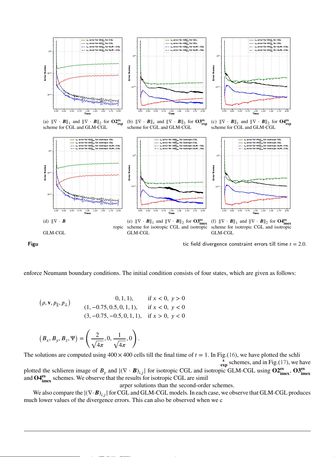
Entropy stable numer ical schemes f or diver g ence diminishing Che w , Goldberg er & Lo w equations f or plasma ﬂow s Chetan Singh a , ∗ , Harish Kumar a,b , Deepak Bhoriya c and Dinsha w S. Balsara d,e a Department of Mathematics, Indian Institute of T echnology Delhi, India b IITD-Abu Dhabi, Abu Dhabi, U AE c Department of Mathematics, BITS-Pilani, Pilani, Rajasthan, India d Physics Department, Univer sity of Notre Dame, USA e A CMS, Univ ersity of Notr e Dame, USA A R T I C L E I N F O Keyw ords : CGL equations GLM-CGL equations GLM technique Entropy stability Diver gence Cleaning Entropy stable numerical schemes A B S T R A C T Chew , Goldberg er & Low (CGL) equations are a set of hyperbolic PDEs with non-conservative products used to model the plasma ﬂows, when the assumption of local thermodynamic equilibrium is not valid, and the pressure tensor is assumed to be rotated by t he magnetic ﬁeld. This results in the pressure tensor, which is described by the two scalar components. As the magnetic ﬁeld also evol ves, controlling t he diver gence of the magnetic ﬁeld is important. In this wor k, we consider the generalized Lagrange multiplier (GLM) technique for the CGL model. The resulting model is referred to as the GLM-CGL system. To make the system suitable for entropy-s table schemes, we reformulate the GLM-CGL system by treating some conservative terms as non-conservative. The resulting system has a non-conservative part t hat does not aﬀect entropy ev olution. W e then propose entropy stable numerical methods for the GLM-CGL model. The numerical results for the GLM-CGL system are then compared wit h the CGL system wit hout the GLM diver gence diminishing approach to demonstrate that t he GLM approach indeed leads to signiﬁcant improv ement in the magnetic ﬁeld divergence diminishing. 1. Introduction MHD has been prov en remarkabl y successful in modelling a wide range of astroph ysical phenomena (see [ 1 , 2 , 3 ]), including planet ary magnetospheres (see [ 4 , 5 , 6 ]), heliosphere (see [ 7 , 8 , 9 ]), astrosphere (see [ 10 , 11 , 12 ]), turbulence (see [ 13 , 14 , 15 ]), and star f ormation (see [ 16 , 17 , 18 ]). MHD assumes local ther modynamic equilibrium for t he plasma, which results in the isotropic pressure. How ev er , for sev eral applications, plasma is eﬀectiv ely collisionless; hence, the pressure cannot be assumed to be isotropic (see [ 19 , 20 , 21 , 22 , 23 , 24 , 25 , 26 , 27 , 28 , 29 , 30 , 31 , 32 , 33 ]). T o o vercome this, Chew , Goldberger and Low’ s equations were ﬁrst introduced in [ 34 ]. The model assumes a gyrotropic descr iption of pressure based on the two scalar pressure components (see [ 35 , 36 , 37 , 33 ]). The CGL equations are hyperbolic in nature and also contain non-conser vativ e terms. Hence, the solutions can be discontinuous and weak solutions need to be considered. For numerical solutions, t he presence of a non-conservative product leads to additional complications as the solution needs to consider a particular pat h (see [ 38 , 39 ]). In practice, how ev er , only linear paths are considered (see [ 33 , 37 ]). In [ 40 ], t he authors present WENO ﬁnite volume schemes for the model. Also, in [ 41 ], an entropy stable discretization is presented. In [ 42 ], the suitability of the CGL model for the heliospheric interface simulations is discussed. More recentl y , in [ 43 ], t he eigen values and the r ight eigen v ectors are presented f or the model. These are then used to design HLL and HLLI appro ximated Riemann solv ers and AFD- WENO schemes [ 44 , 45 ]. For the tw o-dimensional simulations, the solutions of the CGL systems need t o satisfy t he diverg ence-free condition for the magnetic ﬁeld. How ev er, t his is not guaranteed for numerical simulations ev en for MHD equations (see [ 46 , 47 , 48 ]). Hence, several strategies ha ve been dev eloped to o vercome this diﬃculty (see [ 49 , 50 , 51 , 52 , 53 , 54 , 55 , 56 , 57 , 58 , 59 , 60 ]). Fur ther more, similar to the MHD, in CGL equations, the entropy evolution equation inv ol ves diver gence of the magnetic ﬁeld (see [ 41 ]). As t he CGL system is hyperbolic, t he entropy stability of t he numerical ∗ Corresponding author. maz218518@iitd.ac.in (C. Singh); hkumar@iitd.ac.in (H. Kumar); dkbhoriya@gmail.com (D. Bhor iya); dbalsara@nd.edu (D.S. Balsara) OR CI D (s): 0009-0002-6822-8696 (C. Singh) Singh et al.: Preprint submitted to Elsevier Page 1 of 39 Entrop y stable numerical schemes for GLM-CGL system solution is also highly desirable. Hence, two key stability cr iteria for numerical schemes of the CGL equations are diver gence-diminishing/free of the magnetic ﬁeld and entrop y stability . In this ar ticle, our aim is to address these issues using the follo wing steps: • Follo wing the diverg ence diminishing strategy based on t he Generalized Lag range Multiplier (GLM) technique from [ 49 , 51 , 57 , 58 ], we ﬁrst propose the GLM-CGL system. W e t hen analyze the entropy ev olution of GLM- CGL model. • Follo wing [ 41 ], we ref or mulate the system by treating some conservativ e ter ms as non-conser vativ e term, in such a w ay that t he new non-conservative ter ms do not eﬀect entropy production. W e also symmetrize the conser vativ e part by f ollowing [ 61 , 41 , 57 , 58 ]. • T o constr uct diverg ence diminishing entrop y-stable schemes, we ﬁrst design entrop y-conservativ e numer ical ﬂuxes. Following [ 62 ], higher -order numer ical diﬀusion operators are designed using a sign-preserving recon- struction and entropy-scaled eigen vectors. The derivatives in the non-conser vativ e terms are approximated by appropriate central diﬀerence schemes. The whole spatial discretization is prov ed to entropy stable. • For the numer ical validation, sev eral one and two-dimensional problems are considered. In all 2D test cases, we show t hat the GLM approach is beneﬁcial in controlling the diver gence er ror of the magnetic ﬁeld ev olution. The rest of t he ar ticle is organized as f ollow s: In Section 2 , we brieﬂy descr ibe t he CGL equations. In Section 3 , we propose, analyze and reformulate the GLM-CGL system. In Section 4 , we present numerical discretization of the system. In Section 5 , we discuss the fully discrete scheme by presenting time discretization. In Section 6 , numer ical tests are presented. Finall y , we present concluding remarks in Section 7 2. CGL Model The CGL model equations descr ibing the plasma ﬂow are given by (see [ 34 , 35 , 41 , 40 , 43 ]),            v  ∥  𝑩       + ∇ ⋅         v  vv +  ⟂ I + (  ∥ −  ⟂ ) 𝒃𝒃 −  𝑩 𝑩 −  𝑩  2 2 I   ∥ v v   +  ⟂ +  𝑩  2 2  + v ⋅  (  ∥ −  ⟂ ) 𝒃𝒃 − 𝑩 𝑩  v 𝑩 − 𝑩 v        =       0 0 −2  ∥ 𝒃 ⋅ ∇ v ⋅ 𝒃 0 0       . (a) (b) (c) (d) (e) (1) Here , v = (   ,   ,   )  and 𝑩 = (   ,   ,   )  denote density , velocity , and magnetic ﬁelds for the plasma ﬂow . W e denote unit magnetic vector as 𝒃 = (   ,   ,   )  = 𝑩  𝑩  . Using the unit vector , the symmetric pressure tensor 𝑷 is described as, 𝑷 =  ∥ 𝒃𝒃 +  ⟂ ( I − 𝒃𝒃 ) . Here  ∥ is the parallel component and  ⟂ is the perpendicular component of the pressure tensor . W e also deﬁne the a verag e scalar pressure as  = 2  ⟂ +  ∥ 3 . Using this, we close t he system by deﬁning total energy  as follo w s:  = 1 2    v  2 +  𝑩  2 + 3   , (2) In addition, we need to impose diverg ence-free condition on the magnetic ﬁeld, i.e. ∇ ⋅ 𝑩 = 0 . 3. GLM-CGL sys tem One possible approach to control the div ergence er ror is based on the generalized Lag range multiplier (GLM) method (see [ 49 , 51 , 59 ]). For the MHD equations, t he ﬁrst GLM-based reformulation was proposed in [ 51 ]. How ev er , this f or mulation is not consistent wit h t he entropy condition. In t he same work, the authors also introduced an e xtended version of the GLM-based MHD reformulation, referred to as t he EGLM-MHD system . Several aut hors [ 63 , 59 ] hav e also adopted this formulation. Although t his system is consistent with t he entropy condition, t he ninth component of Singh et al.: Preprint submitted to Elsevier P age 2 of 39 Entrop y stable numerical schemes for GLM-CGL system its entropy variable vanishes (see [ 57 ]), which makes t his f or mulation unsuitable for the constr uction of entropy-s table schemes. Sev eral other GLM-based diverg ence-diminishing approaches are considered in [ 64 , 65 , 66 ], but these are also not consistent wit h the entropy condition. More recently , in [ 57 ], authors ha ve proposed an entropy -consistent GLM reformulation of ideal MHD equations. W e f ollow the same f or mulation to ref or mulate the CGL equations. The approach inv ol ves incor porating a Lag range multiplier in the CGL system, namely , an auxiliary scalar ﬁeld Ψ . In t he rest of the article, we use red text to indicate the GLM terms. Follo wing [ 57 ], we introduce the GLM-variable Ψ , which ev olv es as,  Ψ   +   (∇ ⋅ 𝑩 ) + v ⋅ ∇Ψ = 0 , (3) where   is the h yperbolic diverg ence cleaning speed. The transpor t speed of Ψ is taken as the velocity v , consistent with t he velocity acting on B in the ( 1 e). The magnetic ﬁeld equation is now modiﬁed to,  𝑩   + ∇ ⋅ ( v 𝑩 − 𝑩 v +   Ψ I ) = 0 . (4) Follo wing [ 57 ], we note that the scalar Ψ → 0 as ∇ ⋅ 𝑩 → 0 . In addition, all t he red-colored ter ms also vanish, allowing t he model to return to the CGL equations ( 1 ). Thus, the GLM modiﬁcation to the CGL system is consistent. W e also modify the total energy (Eqn. ( 2 )) to reﬂect the contribution of t he GLM-variable Ψ and consider  =  + 1 2 Ψ 2 =   v  2 2 +  𝑩  2 2 + 3  2 + 1 2 Ψ 2 , (5) as the new equation of state wit h the total energy equation as     + ∇ ⋅  v   +  ⟂ +  𝑩  2 2  + v ⋅  (  ∥ −  ⟂ ) 𝒃𝒃 − 𝑩 𝑩  +   Ψ 𝑩  + Ψ v ⋅ ∇Ψ = 0 . (6) Finall y , the GLM-CGL system is given by ,              v  ∥  𝑩 Ψ         + ∇ ⋅                          v  vv +  ⟂ I + (  ∥ −  ⟂ ) 𝒃𝒃 −  𝑩 𝑩 −  𝑩  2 2 I   ∥ v v   +  ⟂ +  𝑩  2 2  + v ⋅  (  ∥ −  ⟂ ) 𝒃𝒃 − 𝑩 𝑩  v 𝑩 − 𝑩 v 0               f   +         0 0 0   Ψ 𝑩   Ψ I   𝑩            f                  +         0 0 0 Ψ v 0 v         ⋅ (∇Ψ)         =         0 0 −2  ∥ 𝒃 ⋅ ∇ v ⋅ 𝒃 0 0 0                 (a) (b) (c) (d) (e) (f) (7) The eigen values of the GLM-CGL system ( 7 ) are presented in Appendix A . 3.1. Entrop y analy sis Let us denote U = ( ,  v ,  ∥ ,  , 𝑩 , Ψ)  to be the conser vativ e variable for the GLM-CGL system. Following [ 41 ], the entropy function is given by  = − . Also, t he entropy ﬂuxes are given by q  =    and q  =    with,  = ln  det 𝑷  5  = ln   ∥  2 ⟂  5  . Then the entropy variable V =    U f or t he GLM-CGL system ( 7 ) is, V =  5 −  −  ⟂  v  2 , 2  ⟂ v , −  ∥ +  ⟂ , − 2  ⟂ , 2  ⟂ 𝑩 , 2  ⟂ Ψ   , (8) where  ⟂ =   ⟂ and  ∥ =   ∥ . W e ha ve the follo wing lemma. Singh et al.: Preprint submitted to Elsevier P age 3 of 39 Entrop y stable numerical schemes for GLM-CGL system Lemma 3.1. The smooth solutions of ( 7 ) satisﬁes    +   q  +   q  + 2  ( v ⋅ 𝑩 )  ⟂ (∇ ⋅ 𝑩 ) = 0 , (9) whic h im plies    +   q  +   q  = 0 , (10) if ∇ ⋅ 𝑩 = 0 . Pr oof. W e ﬁrst note that V  (∇ ⋅ f   ) = −2  ⟂  ∇ ⋅ (   Ψ 𝑩 )  + 2  ⟂ 𝑩  ∇ ⋅ (   Ψ I )  + 2  ⟂ Ψ(∇ ⋅ (   𝑩 )) = −2  ⟂  ∇ ⋅ (   Ψ 𝑩 )  + 2  ⟂ 𝑩  ∇(   Ψ)  + 2  ⟂ Ψ(∇ ⋅ (   𝑩 )) = −2  ⟂  ∇ ⋅ (   Ψ 𝑩 )  + 2  ⟂  ∇ ⋅ (   Ψ 𝑩 )  = 0 . (11) and V     = −2  ⟂ ( Ψ v ⋅ (∇Ψ) ) + 2  ⟂ Ψ ( v ⋅ (∇Ψ) ) = 0 . (12) Furt hermore, from [ 41 ], we hav e V ⋅ (   U + ∇ ⋅ f    −     ) =    +   q  +   q  + 2  ( v ⋅ 𝑩 )  ⟂ (∇ ⋅ 𝑩 ) = 0 . (13) Combining ( 13 ), ( 11 ) and ( 12 ), we get V  ⋅ (   U + ∇ ⋅ ( f    + f   ) +    −     ) =    +   q  +   q  + 2  ( v ⋅ 𝑩 )  ⟂ (∇ ⋅ 𝑩 ) = 0 . (14) W e also note t hat the equality ( 10 ), tur ns into inequality    +   q  +   q  ≤ 0 . (15) f or t he non-smooth solutions. Follo wing [ 57 , 58 ], t he system ( 7 ) is consistent with t he entropy inequality ( 15 ). 3.2. Ref ormulation of the GLM-CGL system Follo wing [ 67 , 41 ], we reformulate the GLM-CGL system by considering some conser vativ e ter ms as non- conservative products. W e get,              v  ∥  𝑩 Ψ         + ∇ ⋅           v  vv +  ⟂ I −  𝑩 𝑩 −  𝑩  2 2 I   ∥ v v   +  ⟂ +  𝑩  2 2  − v ⋅ ( 𝑩 𝑩 ) +   Ψ 𝑩 v 𝑩 − 𝑩 v +   Ψ I   𝑩               f  +         0 0 0 Ψ v 0 v         ⋅ (∇Ψ)         +         0 ∇ ⋅ (  ∥ −  ⟂ ) 𝒃𝒃 2  ∥ 𝒃 ⋅ ∇ v ⋅ 𝒃 ∇ ⋅  v ⋅  (  ∥ −  ⟂ ) 𝒃𝒃  0 0                 = 0 . (a) (b) (c) (d) (e) (f) (16) W e note t hat the choice of non-conservative terms    (blue colored) is such t hat V  ⋅    = 0 (see [ 41 ]). Also, from Eqn. ( 12 ), we already hav e V  ⋅    = 0 . In two dimensions, we can now rewrite t he GLM-CGL system ( 16 ) as f ollow s:  U   +  f    +  f    + Υ   Ψ   + Υ   Ψ   + C  ( U )  U   + C  ( U )  U   = 0 . (17) Singh et al.: Preprint submitted to Elsevier P age 4 of 39 Entrop y stable numerical schemes for GLM-CGL system The ﬂux functions are f  =                   2  +  ⟂ −   2  −  𝑩  2 2      −         −      ∥       +  ⟂ +  𝑩  2 2  −   ( 𝑩 ⋅ v ) +   Ψ     Ψ     −         −                        , f  =                      −      2  +  ⟂ −   2  −  𝑩  2 2      −      ∥       +  ⟂ +  𝑩  2 2  −   ( 𝑩 ⋅ v ) +   Ψ       −       Ψ     −                        . The vectors Υ  , Υ  are deﬁned as Υ  =  0 , 0 , 0 , Ψ   , 0 ,     and Υ  =  0 , 0 , 0 , Ψ   , 0 ,     . The matr ices C  ( U ) and C  ( U ) are given in Appendix B . The conser vativ e ﬂuxes f  and f  are similar to t he GLM-MHD ﬂuxes deﬁned in [ 57 ]. Following [ 67 , 41 ], we note that q  ′ ( U ) = Vf  ′ ( U ) , q  ′ ( U ) = Vf  ′ ( U ) , (18) and V  Υ  = V  Υ  = 0 , (19) Follo wing [ 41 ], we also note t hat V  C  ( U ) = V  C  ( U ) = 0 . (20) Hence, for the system( 17 ), f ollowing [ 67 ], the entropy-entropy ﬂux pair is given by (  , q  , q  ). Fur ther more, we make f ollowing remark about the symmetrizability of the GLM-CGL system: Remar k 3.1. F ollowing [ 41 ], the GLM-CGL syst em is not symmetrizable. 3.3. Symmetrization T o make equations suitable f or the construction of entropy -stable numer ical schemes, we now follo w Godunov’ s process from [ 41 , 68 , 69 , 61 , 57 , 70 ] for t he conser vativ e par t. W e consider ,  U   +  f    +  f    = 0 . (21) Follo wing[ 41 ], we note t hat  f   V ≠   f   V   and  f   V ≠   f   V   , hence the conservative system is not symmetrizable, wit hout assuming ∇ ⋅ 𝑩 = 0 . Follo wing [ 71 , 68 , 69 , 61 , 57 , 70 , 41 ], we rewrite the term 2  ( v ⋅ 𝑩 )  ⟂ using, Φ( V ) = V Φ ′ ( V ) = 2  ( v ⋅ 𝑩 )  ⟂ . (22) Diﬀerentiating, Φ ′ ( V ) = [0 , 𝑩 , 0 , 𝑩 ⋅ v , v , 0 ] . (23) W e also deﬁne the entropy ﬂuxes q  and q  q  = V ⋅ f  + Φ   −   , (24) Singh et al.: Preprint submitted to Elsevier P age 5 of 39 Entrop y stable numerical schemes for GLM-CGL system q  = V ⋅ f  + Φ   −   , (25) with entropy potentials   and     = V ⋅ f  + Φ   − q  = 2   +  ⟂    𝑩  2 + 2    ⟂ Ψ   , (26)   = V ⋅ f  + Φ   − q  = 2   +  ⟂    𝑩  2 + 2    ⟂ Ψ   . (27) Finall y , the Eqn. ( 21 ) is no w symme tr izable if we consider t he term −Φ ′ ( V )  (∇ ⋅ 𝑩 ) on the right-hand side (red colored), which results in              v  ∥  𝑩 Ψ         + ∇ ⋅           v  vv +  ⟂ I −  𝑩 𝑩 −  𝑩  2 2 I   ∥ v v   +  ⟂ +  𝑩  2 2  − v ⋅ ( 𝑩 𝑩 ) +   Ψ 𝑩 v 𝑩 − 𝑩 v +   Ψ I   𝑩          = −         0 𝑩 0 v ⋅ 𝑩 v 0         (∇ ⋅ 𝑩 ) . (a) (b) (c) (d) (e) (f) (28) T ogether with GLM ter ms, we get,  U   +  f    +  f    + Φ ′ ( V )  (∇ ⋅ 𝑩 ) + Υ   Ψ   + Υ   Ψ   = 0 . (29) The system is similar to the GLM-MHD system der iv ed in [ 57 ]. W e fur ther remark that with GLM ter ms, the system ( 29 ) is also symmetrizable. The  -direction eigenv alues of t he system ( 29 ) are,   =    ,   ,   ±   ,   ±   ,   ±   ,   ±    , (30) where  2  =  2   ,  2  = 𝑩 2  ,  2 = 2  ⟂  , and  2  , = 1 2  (  2  +  2 ) ±  (  2  +  2 ) 2 − 4  2   2  . Similarl y , for  -direction,   =    ,   ,   ±   ,   ±   ,   ±   ,   ±    (31) where,  2  =  2   ,  2  = 𝑩 2  ,  2 = 2  ⟂  , and  2  , = 1 2  (  2  +  2 ) ±  (  2  +  2 ) 2 − 4  2   2  . Follo wing [ 68 , 61 , 41 ], we derive and present the entropy-scaled r ight eigen vectors for the system ( 29 ) in t he  - and  -directions in Appendix C . 4. Semi-discret e numerical schemes Combining the Godunov ter ms, GLM terms and additional non-conservative ter ms, we get,  U   +  f    +  f    + Φ ′ ( V )  (∇ ⋅ 𝑩 ) + Υ   Ψ   + Υ   Ψ   + C  ( U )  U   + C  ( U )  U   = 0 . (32) W e will now propose entropy stable numer ical schemes f or these equations using ﬁnite diﬀerence method. Consider a unif or m mesh for the computational domain with cells   of size Δ  × Δ . W e assume t hat the centers of the cell   is denoted by (   ,   ) . The cell vertices are given by (   + 1 2 ,   + 1 2 ) , wit h   + 1 2 =   +   +1 2 and   + 1 2 =   +   +1 2 . A general Singh et al.: Preprint submitted to Elsevier P age 6 of 39 Entrop y stable numerical schemes for GLM-CGL system semi-discrete ﬁnite diﬀerence scheme for ( 32 ) on the uniform mesh is then given by    U , + f , + 1 2 , − f , − 1 2 , Δ  + f ,, + 1 2 − f ,, − 1 2 Δ  + Φ ′ ( V , )          , +        ,  +  (Υ  ) ,   Ψ    , + (Υ  ) ,   Ψ    ,  + C  ( U , )   U    , + C  ( U , )   U    , = 0 . (33) Here, f , + 1 2 , and f ,, + 1 2 are the numer ical ﬂuxes, consistent with the continuous ﬂuxes f  and f  in  - and  -directions, respectiv ely . The der iv atives in non-conservativ e ter ms are discretized with central diﬀerence of appropriate orders (see Appendix D ). For the g rid function  , , let us introduce the notations [ [  ] ]  + 1 2 , =   +1 , −  , , [ [  ] ] , + 1 2 =  , +1 −  , f or t he jumps across t he cell inter faces and    + 1 2 , =   +1 , +  , 2 ,   , + 1 2 =  , +1 +  , 2 , f or t he a verag es across the cell boundaries. 4.1. Entrop y conservativ e schemes Follo wing [ 72 , 61 , 41 ], to design entropy conser vativ e scheme, we ﬁrst need to satisfy t he jump relations, [ [ V ] ]  + 1 2 , ⋅  f , + 1 2 , = [ [   ] ]  + 1 2 , − [ [Φ] ]  + 1 2 ,   , + 1 2 , , (34) [ [ V ] ] , + 1 2 ⋅  f ,, + 1 2 = [ [   ] ] , + 1 2 − [ [Φ] ] , + 1 2   ,, + 1 2 . (35) Follo wing [ 41 ], the entropy conser vativ e ﬂux  f  =    (1)  ,   (2)  ,   (3)  ,   (4)  ,   (5)  ,   (6)  ,   (7)  ,   (8)  ,   (9)  ,   (10)    , is given by ,   (1)  =  ln    ,   (2)  =     ⟂ +      (1)  + 1 2  𝑩  2 −         (3)  =      (1)  −       ,   (4)  =      (1)  −       ,   (5)  =   (1)   ln ∥ ,   (7)  =   Ψ  ⟂   ⟂ ,   (8)  = 1   ⟂   ⟂      −  ⟂       ,   (9)  = 1   ⟂   ⟂      −  ⟂       ,   (10)  =      ,   (6)  = 1 2  2  ln ⟂ −  v  2    (1)  +      (2)  +      (3)  +      (4)  +   (5)  2 +      (7)  +      (8)  +      (9)  − 1 2     𝑩  2 +        +       +           , where  ln = [ [  ] ] [ [ln  ] ] denotes t he logar ithmic av erag e for the scalar g rid function  . W e hav e ignored the spatial indexing to simplify t he notations. Similarly ,  f  , the entropy conservative ﬂux in  -direction can be obt ained. Theref ore, the numer ical scheme ( 33 ) wit h entropy conservative numerical ﬂuxes  f , + 1 2 , =  f  ( U , , U  +1 , ) and  f ,, + 1 2 =  f  ( U , , U , +1 ) is entropy conser vativ e and second-order accurate. W e hav e highlighted the additional terms in red, compared to the numerical ﬂux in [ 41 ]. These ter ms ar ise due to the GLM formulation. Singh et al.: Preprint submitted to Elsevier P age 7 of 39 Entrop y stable numerical schemes for GLM-CGL system T o obtain t he higher -order entropy conservative numer ical schemes, we f ollow [ 73 ] to construct 2   -order accurate ﬂuxes using second-order ﬂux es for an y positive integer  . In par ticular f or (  = 2) , the 4  -order  -directional entropy conservative ﬂux  f 4 , + 1 2 , is given below  f 4 , + 1 2 , = 4 3  f  ( U , , U  +1 , ) − 1 6   f  ( U  −1 , , U  +1 , ) +  f  ( U , , U  +2 , )  . (36) Similarl y , we can der ive t he fourth-order entropy conser vativ e ﬂux  f 4 ,, + 1 2 in  -direction. Again, follo wing [ 41 ], t he numerical scheme ( 33 ) with fourth order numer ical ﬂuxes descr ibed abov e and f our th order discretization of derivativ es of the non-conservative der ivativ e results in a fourth order entropy conser vativ e scheme. 4.2. Entrop y stable schemes T o design entropy-stable numerical schemes, f ollowing [ 72 ], we modify the entropy conser vativ e numer ical ﬂuxes as follo w s  f , + 1 2 , =  f , + 1 2 , − 1 2 D , + 1 2 , [ [ V ] ]  + 1 2 , ,  f ,, + 1 2 =  f ,, + 1 2 − 1 2 D ,, + 1 2 [ [ V ] ] , + 1 2 , (37) where D , + 1 2 , and D ,, + 1 2 are symmetr ic positive deﬁnite matrices. W e use Rusano v’ s type diﬀusion matrices, given by D , + 1 2 , =   , + 1 2 , Λ , + 1 2 ,    , + 1 2 , and D ,, + 1 2 =   ,, + 1 2 Λ ,, + 1 2    ,, + 1 2 , (38) where,    ,  ∈ { ,  } are the matr ices of entropy -scaled right eigen vectors der ived in Appendix C , f ollowing [ 68 , 41 ]. Also, Λ  are, Λ  =  max 1 ≤  ≤ 10       𝐈 10×10 , where {    ∶ 1 ≤  ≤ 10} are given by ( 30 ) and ( 31 ) for t he system ( 29 ) in  and  -directions, respectivel y . T o achiev e higher order, we follo w [ 74 ], to reconstruct scaled entropy variables  ± ,, =    , ± 1 2 , V , , using the ENO procedure, to get the reconstructed polynomials  ± ,, (   ± 1 2 ) of appropr iate order . The ENO procedure has t he sign-preserving property [ 62 ], which ensures t he entropy stability . For the second order . W e use the MinMod limiter , which also has sign-preser ving proper ty . The reconstructed values of scaled entropy variables are given by   ± ,, =  ± ,, (   ± 1 2 ) . Using these, we deﬁne the reconstructed scaled variables as  V ± ,, =     , ± 1 2 ,  (−1)   ± ,, . Finall y , we denote,  f  , + 1 2 , =  f 2  , + 1 2 , − 1 2 D , + 1 2 , [ [  V ] ]  , + 1 2 , . (39) where [ [  V ] ]  , + 1 2 , =  V − , +1 , −  V + ,, . Similarl y , we get,  f  ,, + 1 2 =  f 2  ,, + 1 2 − 1 2 D ,, + 1 2 [ [  V ] ]  ,, + 1 2 . (40) An appropr iate value of  is considered for t he diﬀerent orders of schemes. For t he scheme ( 33 ), we now get, Singh et al.: Preprint submitted to Elsevier P age 8 of 39 Entrop y stable numerical schemes for GLM-CGL system Theorem 4.1 ( see [ 41 ] ) . The scheme using entropy stable ﬂuxes ( 39 ) , ( 40 ) and with second-order (for  = 2 ) and fourth-or der (for  = 3 , 4 ) central diﬀerence appro ximations for        , ,        , ,   Ψ    , ,   Ψ    , ,   U    , , and   U    , is   -or der accurate and entrop y stable (wher e  = 2 , 3 , 4 ), i.e. it satisﬁes     ( U , ) + 1 Δ    q  , + 1 2 , −  q  , − 1 2 ,  + 1 Δ    q  ,, + 1 2 −  q  ,, − 1 2  ≤ 0 , (41) wher e  q   and  q   ar e given by  q  , + 1 2 , =  q 2  , + 1 2 , − 1 2  V   + 1 2 , D , + 1 2 , [ [  V ] ]  , + 1 2 , and  q  ,, + 1 2 =  q 2  ,, + 1 2 − 1 2  V  , + 1 2 D ,, + 1 2 [ [  V ] ]  ,, + 1 2 . T o compute the isotropic limit solutions, we consider t he follo wing source ter m, S =  𝟎 1×4 ,  ⟂ −  ∥  , 𝟎 1×4 , 0   (42) This source relaxes the solution to t he isotropic limit. Here,  is a constant. 5. Time discre tization Let U  be t he solution at  =   and Δ  =   +1 −   . Then the scheme ( 33 ) including the source ter m S ( U , ) , can be represented as,    U , (  ) =  , ( U (  )) + S ( U , (  )) , (43) where,  , ( U (  )) = −  f  , + 1 2 , −  f  , − 1 2 , Δ  −  f  ,, + 1 2 −  f  ,, − 1 2 Δ  − Φ ′ ( V , )          , +        ,  −  (Υ  ) ,   Ψ    , + (Υ  ) ,   Ψ    ,  − C  ( U , )   U    , + C  ( U , )   U    , . When we compute the anisotropic (CGL) solutions, w e do not consider the source term S . So, we use t he explicit SSP-RK methods from [ 75 ]. These schemes are summar ized as follo ws: • O2 es exp ∶ W e take  = 1 for t he entropy conservative numer ical ﬂux. For the diﬀusion operator, we use MinMod -based sign-preser ving reconstr uction. The derivativ es        , ,        , ,   Ψ    , ,   Ψ    , ,   U    , , and   U    , are approximated by second order central diﬀerence. For t he time update, we use the second-order SSP-RK method. • O3 es exp ∶ Here, we take  = 2 f or the entropy conservativ e par t. For the diﬀusion operator, we use t hird-order ENO-based sign-preser ving reconstruction. The derivatives        , ,        , ,   Ψ    , ,   Ψ    , ,   U    , , and   U    , , are appro ximated using f ourt h-order central diﬀerence. For the time update, w e use the t hird-order SSP-RK method. Singh et al.: Preprint submitted to Elsevier P age 9 of 39 Entrop y stable numerical schemes for GLM-CGL system • O4 es exp ∶ Here, we t ake  = 2 for the entropy conser vativ e part.. For the diﬀusion operator , we use f our th-order ENO-based sign-preser ving reconstruction. The derivatives        , ,        , ,   Ψ    , ,   Ψ    , ,   U    , , and   U    , , are approximated using f our th-order central diﬀerence. For t he time update, we use the f our th-order SSP-RK method. T o compute isotr opic (MHD) solutions, we consider the source terms ( 42 ). As low er values of  make the system stiﬀ, we use ARK -IMEX schemes [ 76 , 77 ], where we treat  , ( U (  )) explicitly and S ( U , (  )) implicitly . W e summar ize these schemes as f ollow s: • O2 es imex ∶ The discretization of  , ( U (  )) is same as in t he case of O2 es exp . For t he ARK -IMEX time update, we f ollow , [ 76 ] and consider second-order scheme which is L -stable, where S ( U , (  )) is treated implicitly . • O3 es imex ∶ The discretization of  , ( U (  )) is same as in O3 es exp . The source term S ( U , (  )) is treated implicitly , in the t hird-order ARK -IMEX scheme from [ 77 ]. • O4 es imex ∶ The ter m  , ( U (  )) is discretized as in O4 es exp . W e use fourth order ARK-IMEX scheme from [ 77 ], where we treat S ( U , (  )) , implicitly . 6. Numerical results In this section, we present t he numer ical results for the various one and tw o-dimensional test cases. Following [ 57 , 58 ], we take t he hyperbolic div ergence cleaning speed   =   max  𝚲  − {   +   ,   −   }  ,  ∈ (0 , 1] , f or t he one-dimensional cases. For the tw o-dimensional cases, we take   =   max  𝚲  − {   +   ,   −   } , 𝚲  − {   +   ,   −   }  ,  ∈ (0 , 1] . W e take  = 1 . 0 . The time-step size is estimated as Δ  = CFL max ,    ( U , ) Δ  +   ( U , ) Δ   , where   = max  ∈ 𝚲     and   = max  ∈ 𝚲     . W e take CFL = 0 . 4 for all test cases. For the source terms, we take  = 10 −5 . W e call these solutions as isotr opic GLM-CGL solutions. The solution wit hout the source ter ms is ter med as GLM-CGL solutions. If no GLM diverg ence diminishing is used, t he solution without source ter ms is called CGL solution. Similarly , solutions with source ter ms, but no GLM div ergence diminishing, are termed as isotr opic CGL solutions. T o compare the isotropic solutions and MHD solutions, we hav e computed MHD solutions. For t hat, we use second-order ﬁnite volume methods wit h MinMod-based reconstruction. W e use the Rusano v solv er for t he numer ical ﬂux. For 1D, we use 10000 cells. For 2D, we use highly reﬁned mesh of 1000 × 1000 cells. For tw o-dimensional test cases, to sho w the eﬀect of GLM ter ms on the simulations, we calculate t he div ergence er rors f or t he magnetic ﬁeld in  1 − norm,  ∇ ⋅ 𝑩  1 = 1         =1     =1    (∇ ⋅ 𝑩 ) ,    , and  2 -norm,  ∇ ⋅ 𝑩  2 =     1         =1     =1    (∇ ⋅ 𝑩 ) ,    2     1 2 . Singh et al.: Preprint submitted to Elsevier P age 10 of 39 Entrop y stable numerical schemes for GLM-CGL system Number of cells O2 es exp O3 es exp O4 es exp  1 error Order  1 error Order  1 error Order 12 4.86E-02 – 7.14E-03 – 1.98E-03 – 24 1.51E-02 1.688145847 9.35E-04 2.932342894 2.09E-04 3.241997756 48 6.67E-03 1.176375673 1.18E-04 2.986256366 1.61E-05 3.704200874 96 1.93E-03 1.789540351 1.48E-05 2.996555203 1.16E-06 3.793435746 192 5.32E-04 1.85985482 1.85E-06 2.999133857 8.02E-08 3.852029024 384 1.46E-04 1.863664412 2.31E-07 2.999760591 5.40E-09 3.892946082 T able 1 One-dimensional accuracy test :  1 erro rs and o rder of accuracy for  . Here   and   denote t he number of gr id cells in t he  and  -directions. The discrete diver gence er ror (∇ ⋅ 𝑩 ) , is ev aluated using (∇ ⋅ 𝑩 ) , =  , +1 , −  , −1 , 2Δ  +  ,, +1 −  ,, −1 2Δ  . 6.1. One-dimensional accuracy test In this test case, we demonstrate t he accuracy of t he proposed numer ical schemes for the GLM-CGL system. W e adapt the MHD test problem from [ 78 ]. The computational domain is [0 , 2  ] , with per iodic boundary conditions. The initial data is given as,  ( , 0) = 1 + 0 . 2 sin ,  v ,  ∥ ,  ⟂ , 𝑩 , Ψ  = ( 1 , 0 , 0 , 2 , 2 , 0 . 5 , 1 . 0 , 1 . 5 , 0 ) . W e do not consider t he source term in this test case. The simulations are per formed till time  = 1 . 3 . The exact solution of the problem is  ( ,  ) = 1 + 0 . 2 sin (  −  ) , which is the advection of the density proﬁle with unit velocity in t he  -direction. In T able ( 1 ), we ha ve presented the  1 -er rors and numer ical order of conv erg ence f or density variables, using O2 es exp , O3 es exp and O4 es exp schemes f or the GLM-CGL system. All the schemes ha ve achie ved the predicted order . 6.2. One-dimensional artiﬁcial non-zero magnetic ﬁeld diverg ence test Follo wing [ 57 ], in this test, we consider an initial condition with non-zero diver gence. As numerically , the initial conditions might not hav e a non-zero diver gence of the magnetic ﬁeld (poorl y c hosen initial conditions), we want to present the GLM-CGL framew ork to demonstrate the ability of the method to deal with such a situation. The computational domain is t aken to [−1 , 1] with Neumann boundar y conditions. The magnetic ﬁeld component   is given by ,   =        0 . 0 , if  ≤ −0 . 8 −2(  + 0 . 8) , if − 0 . 8 <  ≤ −0 . 6 exp  − (  ∕0 . 11) 2 2  , if − 0 . 6 <  ≤ 0 . 6 0 . 5 , otherwise. The rest of the variables are taken to be constants and given by ,  , v ,  ∥ ,  ⟂ ,   ,   , Ψ  = ( 1 , 0 , 0 , 0 , 1 , 1 , 0 , 0 , 0 ) . T o demonstrate the eﬀect of GLM-based formulation, we ha ve compared t he GLM-CGL formulation with t he CGL equations without GLM. The numer ical results f or O2 es exp , O3 es exp and O4 es exp schemes for both the f ormulations are presented in Figure ( 1 ) at time  = 0 , 1 , 2 and 3 . For the CGL eq uation wit hout GLM, we obser v e t hat O2 es exp , O3 es exp and O4 es exp schemes (Figures ( 1(a) ), ( 1(b) ) and ( 1(c) )) preser v e the initial proﬁle of t he  − magnetic ﬁeld component (   ) . So, the diver gence of the initial proﬁle is not diminished. W e observe only slight diﬀusion in the   proﬁle ov er time. Singh et al.: Preprint submitted to Elsevier P age 11 of 39 Entrop y stable numerical schemes for GLM-CGL system 1.00 0.75 0.50 0.25 0.00 0.25 0.50 0.75 1.00 0.4 0.2 0.0 0.2 0.4 0.6 0.8 1.0 t = 0 t = 1 t = 2 t = 3 (a)   f or O2 es exp scheme for CGL 1.00 0.75 0.50 0.25 0.00 0.25 0.50 0.75 1.00 0.4 0.2 0.0 0.2 0.4 0.6 0.8 1.0 t = 0 t = 1 t = 2 t = 3 (b)   f or O3 es exp scheme for CGL 1.00 0.75 0.50 0.25 0.00 0.25 0.50 0.75 1.00 0.4 0.2 0.0 0.2 0.4 0.6 0.8 1.0 t = 0 t = 1 t = 2 t = 3 (c)   f or O4 es exp scheme for CGL 1.00 0.75 0.50 0.25 0.00 0.25 0.50 0.75 1.00 0.4 0.2 0.0 0.2 0.4 0.6 0.8 1.0 t = 0 t = 1 t = 2 t = 3 (d)   f or O2 es exp scheme for GLM-CGL 1.00 0.75 0.50 0.25 0.00 0.25 0.50 0.75 1.00 0.4 0.2 0.0 0.2 0.4 0.6 0.8 1.0 t = 0 t = 1 t = 2 t = 3 (e)   f or O3 es exp scheme for GLM-CGL 1.00 0.75 0.50 0.25 0.00 0.25 0.50 0.75 1.00 0.4 0.2 0.0 0.2 0.4 0.6 0.8 1.0 t = 0 t = 1 t = 2 t = 3 (f)   f or O4 es exp scheme for GLM- CGL Figure 1: One-dimensional artiﬁcial non-zero magnetic ﬁeld divergence test : Plots of magnetic ﬁeld evolution fo r O2 es exp , O3 es exp and O4 es exp schemes for CGL and GLM-CGL at four diﬀerent time steps. In Figures ( 1(d) ), ( 1(e) ) and ( 1(f) ), we hav e plotted the magnetic ﬁeld ev olution   f or the O2 es exp , O3 es exp and O4 es exp schemes f or GLM-CGL. In this case, we obser ve that as time increases, t he diver gence of the magnetic ﬁeld decreases and becomes zero at  = 3 . This demonstrates that the GLM-CGL f ormulation deals with the diverg ence eﬀectivel y , ev en in a one-dimensional case. W e also observe t hat all the numer ical schemes beha ve similarly , with higher-or der schemes being less diﬀusive. Fur ther more, the results are comparable to those obt ained in [ 57 ] for MHD equations. 6.3. Brio- W u shock tube problem In this test, we generalize the Brio-W u shock tube test case f or MHD equations [ 79 ]. The test was also considered in [ 41 , 43 ]. Follo wing [ 41 ], we t ake t he computational domain to be [−1 , 1] with Neumann boundary conditions. The initial conditions are: ( , v ,  ∥ ,  ⟂ ,   ,   ,   , Ψ) =  (1 , 0 , 0 , 0 , 1 , 1 , 0 . 75 , 1 , 0 , 0) , if  ≤ 0 (0 . 125 , 0 , 0 , 0 , 0 . 1 , 0 . 1 , 0 . 75 , −1 , 0 , 0) , otherwise In Figure ( 2 ), we present the numer ical results at time  = 0 . 2 for CGL and GLM-CGL formulations. W e also consider t he isotropic CGL and isotropic GLM-CGL by considering the source term and using IMEX schemes O2 es imex , O3 es imex and O4 es imex . The simulations use 2000 cells. W e ha ve also compared MHD and isotropic solutions. W e hav e plotted proﬁles of density ,  ∥ and  ⟂ f or all the test cases. For t he CGL and GLM-CGL, we obser v e that all schemes successfully resolv e the wa v es. W e obser ve small-scale oscillations (similar to t hose in [ 41 ]), but t hey decrease with fur ther reﬁnements. W e also obser v e that t he GLM-CGL solutions are slightly more diﬀusiv e t han the CGL solutions f or the same order of scheme. For t he isotropic cases, we note t hat both  ∥ and  ⟂ ha ve the same proﬁle (whic h matches the MHD pressure proﬁle), as expected. Fur ther more, the density proﬁle matches the MHD density proﬁle. Fur ther more, we again see that isotropic GLM-CGL solutions are slightly more diﬀusiv e t han the isotropic CGL solution. In all the cases, we also observe that higher -order schemes are more accurate. Singh et al.: Preprint submitted to Elsevier P age 12 of 39 Entrop y stable numerical schemes for GLM-CGL system 1.00 0.75 0.50 0.25 0.00 0.25 0.50 0.75 1.00 0.2 0.4 0.6 0.8 1.0 O 2 e s e x p f o r C G L O 2 e s e x p f o r G L M - C G L O 3 e s e x p f o r C G L O 3 e s e x p f o r G L M - C G L O 4 e s e x p f o r C G L O 4 e s e x p f o r G L M - C G L 0.10 0.05 0.00 0.625 0.650 0.675 0.700 (a) Density for explicit schemes for CGL and GLM-CGL 1.00 0.75 0.50 0.25 0.00 0.25 0.50 0.75 1.00 0.2 0.4 0.6 0.8 1.0 O 2 e s e x p f o r C G L O 2 e s e x p f o r G L M - C G L O 3 e s e x p f o r C G L O 3 e s e x p f o r G L M - C G L O 4 e s e x p f o r C G L O 4 e s e x p f o r G L M - C G L (b)  ∥ f or explicit schemes for CGL and GLM-CGL 1.00 0.75 0.50 0.25 0.00 0.25 0.50 0.75 1.00 0.2 0.4 0.6 0.8 1.0 O 2 e s e x p f o r C G L O 2 e s e x p f o r G L M - C G L O 3 e s e x p f o r C G L O 3 e s e x p f o r G L M - C G L O 4 e s e x p f o r C G L O 4 e s e x p f o r G L M - C G L (c)  ⟂ f or explicit schemes for CGL and GLM-CGL 1.00 0.75 0.50 0.25 0.00 0.25 0.50 0.75 1.00 0.2 0.4 0.6 0.8 1.0 MHD O 2 e s i m e x f o r i s o t r o p i c C G L O 2 e s i m e x f o r i s o t r o p i c G L M - C G L O 3 e s i m e x f o r i s o t r o p i c C G L O 3 e s i m e x f o r i s o t r o p i c G L M - C G L O 4 e s i m e x f o r i s o t r o p i c C G L O 4 e s i m e x f o r i s o t r o p i c G L M - C G L 0.10 0.08 0.06 0.04 0.02 0.00 0.7 0.8 0.9 (d) Density f or IMEX schemes for isotropic CGL and isotropic GLM-CGL 1.00 0.75 0.50 0.25 0.00 0.25 0.50 0.75 1.00 0.2 0.4 0.6 0.8 1.0 MHD O 2 e s i m e x f o r i s o t r o p i c C G L O 2 e s i m e x f o r i s o t r o p i c G L M - C G L O 3 e s i m e x f o r i s o t r o p i c C G L O 3 e s i m e x f o r i s o t r o p i c G L M - C G L O 4 e s i m e x f o r i s o t r o p i c C G L O 4 e s i m e x f o r i s o t r o p i c G L M - C G L (e)  ∥ f or IMEX schemes for isotropic CGL and isotropic GLM-CGL 1.00 0.75 0.50 0.25 0.00 0.25 0.50 0.75 1.00 0.2 0.4 0.6 0.8 1.0 MHD O 2 e s i m e x f o r i s o t r o p i c C G L O 2 e s i m e x f o r i s o t r o p i c G L M - C G L O 3 e s i m e x f o r i s o t r o p i c C G L O 3 e s i m e x f o r i s o t r o p i c G L M - C G L O 4 e s i m e x f o r i s o t r o p i c C G L O 4 e s i m e x f o r i s o t r o p i c G L M - C G L (f)  ⟂ f or IMEX sc hemes for isotropic CGL and isotropic GLM-CGL Figure 2: Brio-Wu sho ck tube p roblem : Plots of density , parallel and perp endicular pressure comp onents fo r explicit schemes and IMEX schemes using 2000 cells at ﬁnal time  = 0 . 2 . Number of cells O2 es exp O3 es exp O4 es exp  1 error Order  1 error Order  1 error Order 24 × 24 2.22E-02 – 1.47E-03 – 3.29E-04 – 48 × 48 9.66E-03 1.197102245 1.88E-04 2.97345722 2.60E-05 3.665723172 96 × 96 3.00E-03 1.685415758 2.35E-05 2.995912704 1.87E-06 3.79493394 192 × 192 8.43E-04 1.834041352 2.94E-06 2.999439213 1.30E-07 3.845890159 384 × 384 2.32E-04 1.858969497 3.68E-07 2.999783442 8.78E-09 3.888987053 T able 2 T wo-dimensional accuracy test :  1 erro rs and o rder of accuracy for  . 6.4. T wo-dimensional accuracy test For the tw o-dimensional accuracy test, we g eneralize the one-dimensional accuracy test in Section 6.1 to two dimensions for the GLM-CGL system. W e consider the computational domain [0 , 2  ] × [0 , 2  ] with periodic boundar y conditions. The initial conditions are given below ,  ( , , 0) = 1 + 0 . 2 sin (  +  ) ,  v ,  ∥ ,  ⟂ , 𝑩 , Ψ  = ( 0 . 5 , 0 . 5 , 0 , 2 , 2 , 0 . 5 , 1 . 0 , 1 . 5 , 0 ) . The ex act solution is then given by  ( , ,  ) = 1 + 0 . 2 sin (  +  −  ) . For the O2 es exp , O3 es exp and O4 es exp schemes with GLM, the  1 -er rors of the density are shown in Table( 2 ) at the ﬁnal time of  = 1 . 3 . W e note that all the schemes con ver ge with t he theoretically predicted order of accuracy . 6.5. T wo-dimensional Circularly polarized Alfv én wa v es T o test the accuracy of the magnetic ﬁeld components, in this test we consider the generalization of the tw o- dimensional MHD circularly polar ized alfvén w a ves problem, which was introduced in [ 80 ], for the GLM-CGL system. W e consider the comput ational domain is  0 , 1 cos   ×  0 , 1 sin   , with per iodic boundar y conditions. The initial condition Singh et al.: Preprint submitted to Elsevier P age 13 of 39 Entrop y stable numerical schemes for GLM-CGL system Number of cells O2 es exp O3 es exp O4 es exp  1 error Order  1 error Order  1 error Order 32 × 32 2.53E-02 – 1.25E-03 – 2.92E-04 – 64 × 64 8.06E-03 1.649122178 1.57E-04 2.997015955 2.39E-05 3.606907328 128 × 128 3.49E-03 1.208907716 2.01E-05 2.964144554 1.69E-06 3.825756677 256 × 256 9.84E-04 1.824933152 2.55E-06 2.978762804 1.13E-07 3.898604125 512 × 512 2.75E-04 1.840806962 3.26E-07 2.965870547 6.36E-09 4.153053838 T able 3 T wo-dimensional Circularly p olarized Alfvén waves :  1 erro rs and o rder of accuracy for   . is given as  ,  ∥ ,  ⟂ , Ψ  = ( 1 , 0 . 1 , 0 . 1 , 0 ) , v =  −  ⟂ sin  ,  ⟂ cos  , 0 . 1 cos (2    )  , 𝑩 =    cos  −  ⟂ sin  ,   sin  +  ⟂ cos  ,    , where   = 1 ,  ⟂ =  ⟂ = 0 . 1 sin (2    ) and   =  cos  +  sin  . Circularl y polarized alfvén wa ve hav e a unit w av elength in the direction of the  -axis and propagate at an angle  = 30  . For the GLM-CGL with O2 es exp , O3 es exp and O4 es exp schemes, the  1 -er rors of   are sho wn in T able( 3 ). W e note that ev er y scheme has the desired order of accuracy . 6.6. Orszag- T ang Problem Follo wing the Orszag- T ang problem f or MHD [ 81 , 80 , 61 ], we present a generalized version of the problem for the GLM-CGL (see [ 41 ]). The domain for the problem is [0 , 1] × [0 , 1] , with per iodic boundar y conditions. The initial state is giv en as,  ,  ∥ ,  ⟂ , Ψ  =  25 36  , 5 12  , 5 12  , 0  , v = ( − sin (2   ) , sin (2   ) , 0 ) , 𝑩 = 1  4  ( − sin (2   ) , sin (4   ) , 0 ) . It was obser ved in [ 41 , 40 ] that the CGL model without the source ter m (anisotropic case) has diﬃculty in simulating this test case. Hence, we consider t he isotropic CGL and isotropic GLM-CGL cases only . This also makes the solution suitable to compare with the MHD solution. The numer ical results are presented in Figures ( 3 ), ( 4 ) and ( 5 ). W e hav e used 400 × 400 cells and simulated till the ﬁnal time  = 0 . 5 , using t he numerical schemes O2 es imex , O3 es imex and O4 es imex . From t he 2D density plots, we do not see any signiﬁcant diﬀerence betw een the solutions. How ev er, to obser ve more closely , we ha ve plotted a one-dimensional cut plot at  = 0 . 3125 of density and  ⟂ f or diﬀerent schemes and compared with the MHD solutions. All t he solutions are similar to the MHD solutions. W e obser ve t hat all schemes produce solutions that are close to t he MHD solution. W e furt her obser v e t hat GLM-CGL solutions are slightly more diﬀusiv e when compared with CGL solutions of t he same order . The numer ical results are presented in Figures ( 3 ), ( 4 ) and ( 5 ). W e hav e used 400 × 400 cells and simulated till the ﬁnal time  = 0 . 5 , using t he numerical schemes O2 es imex , O3 es imex and O4 es imex . From t he 2D density plots, we do not see any signiﬁcant diﬀerence betw een the solutions. How ev er, to obser ve more closely , we ha ve plotted a one-dimensional cut plot at  = 0 . 3125 of density and  ⟂ f or diﬀerent schemes and compared with t he MHD solutions. All the isotropic solutions are close to t he MHD solution. W e fur ther observe that GLM-CGL solutions are slightly more diﬀusiv e when compared with CGL solutions of the same order . In Figure ( 3 ), we obser ved that t he diverg ence er rors for the GLM-CGL model are signiﬁcantly low er than the CGL model (almost one-third) for all the schemes. This is fur ther obser ved in the Figure ( 4 ), where we hav e plotted the time ev olution of t he  1 and  2 er rors for diverg ence of t he magnetic ﬁeld. W e again obser ve that the GLM-CGL diver gence er rors are signiﬁcantly lower t han the CGL case, f or all orders. Singh et al.: Preprint submitted to Elsevier P age 14 of 39 Entrop y stable numerical schemes for GLM-CGL system 0.2 0.4 0.6 0.8 x 0.2 0.4 0.6 0.8 y 0.12 0.16 0.20 0.24 0.28 0.32 0.36 0.40 0.44 (a) Density for O2 es imex scheme for isotropic CGL 0.2 0.4 0.6 0.8 x 0.2 0.4 0.6 0.8 y 0.12 0.16 0.20 0.24 0.28 0.32 0.36 0.40 0.44 (b) Density for O3 es imex scheme for isotropic CGL 0.2 0.4 0.6 0.8 x 0.2 0.4 0.6 0.8 y 0.12 0.16 0.20 0.24 0.28 0.32 0.36 0.40 0.44 0.48 (c) Density for O4 es imex scheme for isotropic CGL 0.2 0.4 0.6 0.8 x 0.2 0.4 0.6 0.8 y 0.12 0.16 0.20 0.24 0.28 0.32 0.36 0.40 0.44 (d) Density for O2 es imex scheme for isotropic GLM-CGL 0.2 0.4 0.6 0.8 x 0.2 0.4 0.6 0.8 y 0.12 0.16 0.20 0.24 0.28 0.32 0.36 0.40 0.44 (e) Density for O3 es imex scheme for isotropic GLM-CGL 0.2 0.4 0.6 0.8 x 0.2 0.4 0.6 0.8 y 0.12 0.16 0.20 0.24 0.28 0.32 0.36 0.40 0.44 (f) Density for O4 es imex scheme for isotropic GLM-CGL 0.2 0.4 0.6 0.8 x 0.2 0.4 0.6 0.8 y 1.5 3.0 4.5 6.0 7.5 9.0 10.5 12.0 13.5 (g)  (∇ ⋅ 𝑩 ) ,  for O2 es imex scheme f or isotropic CGL 0.2 0.4 0.6 0.8 x 0.2 0.4 0.6 0.8 y 3 6 9 12 15 18 21 24 27 (h)  (∇ ⋅ 𝑩 ) ,  for O3 es imex scheme f or isotropic CGL 0.2 0.4 0.6 0.8 x 0.2 0.4 0.6 0.8 y 3 6 9 12 15 18 21 24 27 (i)  (∇ ⋅ 𝑩 ) ,  for O4 es imex scheme for isotropic CGL 0.2 0.4 0.6 0.8 x 0.2 0.4 0.6 0.8 y 0.2 0.4 0.6 0.8 1.0 1.2 1.4 1.6 (j)  (∇ ⋅ 𝑩 ) ,  for O2 es imex scheme for isotropic GLM-CGL 0.2 0.4 0.6 0.8 x 0.2 0.4 0.6 0.8 y 0.8 1.6 2.4 3.2 4.0 4.8 5.6 6.4 (k)  (∇ ⋅ 𝑩 ) ,  for O3 es imex scheme f or isotropic GLM-CGL 0.2 0.4 0.6 0.8 x 0.2 0.4 0.6 0.8 y 0.8 1.6 2.4 3.2 4.0 4.8 5.6 6.4 (l)  (∇ ⋅ 𝑩 ) ,  for O4 es imex scheme for isotropic GLM-CGL Figure 3: Orszag-T ang Problem : Plots of densit y and  (∇ ⋅ 𝑩 ) ,  fo r O2 es imex , O3 es imex and O4 es imex schemes fo r isotropic CGL and isotropic GLM-CGL at time  = 0 . 5 . Singh et al.: Preprint submitted to Elsevier P age 15 of 39 Entrop y stable numerical schemes for GLM-CGL system 0.0 0.1 0.2 0.3 0.4 0.5 T i m e 1 0 4 1 0 3 1 0 2 1 0 1 1 0 0 E r r o r N o r m s L 1 e r r o r f o r O 2 e s i m e x f o r i s o t r o p i c C G L L 2 e r r o r f o r O 2 e s i m e x f o r i s o t r o p i c C G L L 1 e r r o r f o r O 2 e s i m e x f o r i s o t r o p i c G L M C G L L 2 e r r o r f o r O 2 e s i m e x f o r i s o t r o p i c G L M C G L (a)  ∇ ⋅ 𝑩  1 and  ∇ ⋅ 𝑩  2 f or O2 es imex scheme f or isotropic CGL and isotropic GLM-CGL 0.0 0.1 0.2 0.3 0.4 0.5 T i m e 1 0 4 1 0 3 1 0 2 1 0 1 1 0 0 E r r o r N o r m s L 1 e r r o r f o r O 3 e s i m e x f o r i s o t r o p i c C G L L 2 e r r o r f o r O 3 e s i m e x f o r i s o t r o p i c C G L L 1 e r r o r f o r O 3 e s i m e x f o r i s o t r o p i c G L M C G L L 2 e r r o r f o r O 3 e s i m e x f o r i s o t r o p i c G L M C G L (b)  ∇ ⋅ 𝑩  1 and  ∇ ⋅ 𝑩  2 f or O3 es imex scheme f or isotropic CGL and isotropic GLM-CGL 0.0 0.1 0.2 0.3 0.4 0.5 T i m e 1 0 4 1 0 3 1 0 2 1 0 1 1 0 0 E r r o r N o r m s L 1 e r r o r f o r O 4 e s i m e x f o r i s o t r o p i c C G L L 2 e r r o r f o r O 4 e s i m e x f o r i s o t r o p i c C G L L 1 e r r o r f o r O 4 e s i m e x f o r i s o t r o p i c G L M C G L L 2 e r r o r f o r O 4 e s i m e x f o r i s o t r o p i c G L M C G L (c)  ∇ ⋅ 𝑩  1 and  ∇ ⋅ 𝑩  2 f or O4 es imex scheme f or isotropic CGL and isotropic GLM-CGL Figure 4: Orszag-T ang Problem : Evolution of the magnetic ﬁeld divergence constraint errors till time  = 0 . 5 . 0.0 0.2 0.4 0.6 0.8 1.0 x-axis 0.05 0.10 0.15 0.20 0.25 p MHD O 2 e s i m e x f o r i s o t r o p i c C G L O 2 e s i m e x f o r i s o t r o p i c G L M - C G L O 3 e s i m e x f o r i s o t r o p i c C G L O 3 e s i m e x f o r i s o t r o p i c G L M - C G L O 4 e s i m e x f o r i s o t r o p i c C G L O 4 e s i m e x f o r i s o t r o p i c G L M - C G L 0.060 0.065 0.070 0.075 0.080 0.085 0.090 0.095 0.100 0.18 0.20 0.22 0.24 Zoom (a) Cut of pressure component  ∥ f or isotropic CGL and isotropic GLM-CGL along  = 0 . 3125 0.0 0.2 0.4 0.6 0.8 1.0 x-axis 0.05 0.10 0.15 0.20 0.25 p MHD O 2 e s i m e x f o r i s o t r o p i c C G L O 2 e s i m e x f o r i s o t r o p i c G L M - C G L O 3 e s i m e x f o r i s o t r o p i c C G L O 3 e s i m e x f o r i s o t r o p i c G L M - C G L O 4 e s i m e x f o r i s o t r o p i c C G L O 4 e s i m e x f o r i s o t r o p i c G L M - C G L 0.060 0.065 0.070 0.075 0.080 0.085 0.090 0.095 0.100 0.18 0.20 0.22 0.24 Zoom (b) Cut of pressure component  ⟂ f or isotropic CGL and isotropic GLM-CGL along  = 0 . 3125 Figure 5: Orszag-T ang Problem : Cut plots of pressure components along  = 0 . 3125 at time  = 0 . 5 . Singh et al.: Preprint submitted to Elsevier P age 16 of 39 Entrop y stable numerical schemes for GLM-CGL system 0.2 0.4 0.6 0.8 x 0.2 0.4 0.6 0.8 y 0.08 0.16 0.24 0.32 0.40 0.48 0.56 0.64 0.72 (a)  ⟂ f or O2 es exp scheme for CGL 0.2 0.4 0.6 0.8 x 0.2 0.4 0.6 0.8 y 0.08 0.16 0.24 0.32 0.40 0.48 0.56 0.64 0.72 0.80 (b)  ⟂ f or O3 es exp scheme for CGL 0.2 0.4 0.6 0.8 x 0.2 0.4 0.6 0.8 y 0.08 0.16 0.24 0.32 0.40 0.48 0.56 0.64 0.72 0.80 (c)  ⟂ f or O4 es exp scheme for CGL 0.2 0.4 0.6 0.8 x 0.2 0.4 0.6 0.8 y 0.08 0.16 0.24 0.32 0.40 0.48 0.56 0.64 0.72 (d)  ⟂ f or O2 es exp scheme for GLM- CGL 0.2 0.4 0.6 0.8 x 0.2 0.4 0.6 0.8 y 0.1 0.2 0.3 0.4 0.5 0.6 0.7 0.8 (e)  ⟂ f or O3 es exp scheme for GLM- CGL 0.2 0.4 0.6 0.8 x 0.2 0.4 0.6 0.8 y 0.1 0.2 0.3 0.4 0.5 0.6 0.7 0.8 (f)  ⟂ f or O4 es exp scheme f or GLM- CGL 0.2 0.4 0.6 0.8 x 0.2 0.4 0.6 0.8 y 0.0 1.5 3.0 4.5 6.0 7.5 9.0 10.5 (g)  (∇ ⋅ 𝑩 ) ,  for O2 es exp scheme for CGL 0.2 0.4 0.6 0.8 x 0.2 0.4 0.6 0.8 y 0.0 2.5 5.0 7.5 10.0 12.5 15.0 17.5 20.0 (h)  (∇ ⋅ 𝑩 ) ,  for O3 es exp scheme for CGL 0.2 0.4 0.6 0.8 x 0.2 0.4 0.6 0.8 y 0 3 6 9 12 15 18 21 24 (i)  (∇ ⋅ 𝑩 ) ,  f or O4 es exp scheme for CGL 0.2 0.4 0.6 0.8 x 0.2 0.4 0.6 0.8 y 0.2 0.4 0.6 0.8 1.0 1.2 1.4 1.6 1.8 (j)  (∇ ⋅ 𝑩 ) ,  f or O2 es exp scheme for GLM-CGL 0.2 0.4 0.6 0.8 x 0.2 0.4 0.6 0.8 y 0.3 0.6 0.9 1.2 1.5 1.8 2.1 2.4 2.7 (k)  (∇ ⋅ 𝑩 ) ,  for O3 es exp scheme for GLM-CGL 0.2 0.4 0.6 0.8 x 0.2 0.4 0.6 0.8 y 0.6 1.2 1.8 2.4 3.0 3.6 4.2 4.8 (l)  (∇ ⋅ 𝑩 ) ,  f or O4 es exp scheme for GLM-CGL Figure 6: Rotor problem : Plots of  ⟂ and  (∇ ⋅ 𝑩 ) ,  for O2 es exp , O3 es exp and O4 es exp schemes for CGL and GLM-CGL at time  = 0 . 295 . Singh et al.: Preprint submitted to Elsevier P age 17 of 39 Entrop y stable numerical schemes for GLM-CGL system 0.2 0.4 0.6 0.8 x 0.2 0.4 0.6 0.8 y 0.08 0.16 0.24 0.32 0.40 0.48 0.56 0.64 0.72 (a)  ⟂ f or O2 es imex scheme for isotropic CGL 0.2 0.4 0.6 0.8 x 0.2 0.4 0.6 0.8 y 0.08 0.16 0.24 0.32 0.40 0.48 0.56 0.64 0.72 (b)  ⟂ f or O3 es imex scheme f or isotropic CGL 0.2 0.4 0.6 0.8 x 0.2 0.4 0.6 0.8 y 0.08 0.16 0.24 0.32 0.40 0.48 0.56 0.64 0.72 (c)  ⟂ f or O4 es imex scheme for isotropic CGL 0.2 0.4 0.6 0.8 x 0.2 0.4 0.6 0.8 y 0.08 0.16 0.24 0.32 0.40 0.48 0.56 0.64 0.72 (d)  ⟂ f or O2 es imex scheme f or isotropic GLM-CGL 0.2 0.4 0.6 0.8 x 0.2 0.4 0.6 0.8 y 0.08 0.16 0.24 0.32 0.40 0.48 0.56 0.64 0.72 (e)  ⟂ f or O3 es imex scheme for isotropic GLM-CGL 0.2 0.4 0.6 0.8 x 0.2 0.4 0.6 0.8 y 0.08 0.16 0.24 0.32 0.40 0.48 0.56 0.64 0.72 (f)  ⟂ f or O4 es imex scheme for isotropic GLM-CGL 0.2 0.4 0.6 0.8 x 0.2 0.4 0.6 0.8 y 0 2 4 6 8 10 12 14 16 (g)  (∇ ⋅ 𝑩 ) ,  for O2 es imex scheme f or isotropic CGL 0.2 0.4 0.6 0.8 x 0.2 0.4 0.6 0.8 y 0.0 2.5 5.0 7.5 10.0 12.5 15.0 17.5 20.0 22.5 (h)  (∇ ⋅ 𝑩 ) ,  for O3 es imex scheme f or isotropic CGL 0.2 0.4 0.6 0.8 x 0.2 0.4 0.6 0.8 y 0 3 6 9 12 15 18 21 24 27 (i)  (∇ ⋅ 𝑩 ) ,  for O4 es imex scheme for isotropic CGL 0.2 0.4 0.6 0.8 x 0.2 0.4 0.6 0.8 y 0.15 0.30 0.45 0.60 0.75 0.90 1.05 (j)  (∇ ⋅ 𝑩 ) ,  for O2 es imex scheme for isotropic GLM-CGL 0.2 0.4 0.6 0.8 x 0.2 0.4 0.6 0.8 y 0.3 0.6 0.9 1.2 1.5 1.8 2.1 2.4 2.7 (k)  (∇ ⋅ 𝑩 ) ,  for O3 es imex scheme f or isotropic GLM-CGL 0.2 0.4 0.6 0.8 x 0.2 0.4 0.6 0.8 y 0.5 1.0 1.5 2.0 2.5 3.0 3.5 4.0 4.5 (l)  (∇ ⋅ 𝑩 ) ,  for O4 es imex scheme for isotropic GLM-CGL Figure 7: Rotor problem : Plots of  ⟂ and  (∇ ⋅ 𝑩 ) ,  for O2 es imex , O3 es imex and O4 es imex schemes for isotropic CGL and isotropic GLM-CGL at time  = 0 . 295 . Singh et al.: Preprint submitted to Elsevier P age 18 of 39 Entrop y stable numerical schemes for GLM-CGL system 0.0 0.2 0.4 0.6 0.8 1.0 x-axis 0.0 0.1 0.2 0.3 0.4 0.5 0.6 0.7 p MHD O 2 e s i m e x f o r i s o t r o p i c C G L O 2 e s i m e x f o r i s o t r o p i c G L M - C G L O 3 e s i m e x f o r i s o t r o p i c C G L O 3 e s i m e x f o r i s o t r o p i c G L M - C G L O 4 e s i m e x f o r i s o t r o p i c C G L O 4 e s i m e x f o r i s o t r o p i c G L M - C G L (a) Cut of pressure component  ∥ f or isotropic CGL and isotropic GLM-CGL along  = 0 . 489 using 400 × 400 cells 0.0 0.2 0.4 0.6 0.8 1.0 x-axis 0.0 0.1 0.2 0.3 0.4 0.5 0.6 0.7 p MHD O 2 e s i m e x f o r i s o t r o p i c C G L O 2 e s i m e x f o r i s o t r o p i c G L M - C G L O 3 e s i m e x f o r i s o t r o p i c C G L O 3 e s i m e x f o r i s o t r o p i c G L M - C G L O 4 e s i m e x f o r i s o t r o p i c C G L O 4 e s i m e x f o r i s o t r o p i c G L M - C G L (b) Cut of pressure component  ⟂ f or isotropic CGL and isotropic GLM-CGL along  = 0 . 489 using 400 × 400 cells Figure 8: Rotor problem : Cut plot of pressure components  ∥ and  ⟂ at time  = 0 . 295 . 0.00 0.05 0.10 0.15 0.20 0.25 0.30 T i m e 1 0 3 1 0 2 1 0 1 E r r o r N o r m s L 1 e r r o r f o r O 2 e s e x p f o r C G L L 2 e r r o r f o r O 2 e s e x p f o r C G L L 1 e r r o r f o r O 2 e s e x p f o r G L M C G L L 2 e r r o r f o r O 2 e s e x p f o r G L M C G L (a)  ∇ ⋅ 𝑩  1 and  ∇ ⋅ 𝑩  2 f or O2 es exp scheme for CGL and GLM-CGL 0.00 0.05 0.10 0.15 0.20 0.25 0.30 T i m e 1 0 3 1 0 2 1 0 1 1 0 0 E r r o r N o r m s L 1 e r r o r f o r O 3 e s e x p f o r C G L L 2 e r r o r f o r O 3 e s e x p f o r C G L L 1 e r r o r f o r O 3 e s e x p f o r G L M C G L L 2 e r r o r f o r O 3 e s e x p f o r G L M C G L (b)  ∇ ⋅ 𝑩  1 and  ∇ ⋅ 𝑩  2 f or O3 es exp scheme for CGL and GLM-CGL 0.00 0.05 0.10 0.15 0.20 0.25 0.30 T i m e 1 0 3 1 0 2 1 0 1 1 0 0 E r r o r N o r m s L 1 e r r o r f o r O 4 e s e x p f o r C G L L 2 e r r o r f o r O 4 e s e x p f o r C G L L 1 e r r o r f o r O 4 e s e x p f o r G L M C G L L 2 e r r o r f o r O 4 e s e x p f o r G L M C G L (c)  ∇ ⋅ 𝑩  1 and  ∇ ⋅ 𝑩  2 f or O4 es exp scheme for CGL and GLM-CGL 0.00 0.05 0.10 0.15 0.20 0.25 0.30 T i m e 1 0 3 1 0 2 1 0 1 E r r o r N o r m s L 1 e r r o r f o r O 2 e s i m e x f o r i s o t r o p i c C G L L 2 e r r o r f o r O 2 e s i m e x f o r i s o t r o p i c C G L L 1 e r r o r f o r O 2 e s i m e x f o r i s o t r o p i c G L M C G L L 2 e r r o r f o r O 2 e s i m e x f o r i s o t r o p i c G L M C G L (d)  ∇ ⋅ 𝑩  1 and  ∇ ⋅ 𝑩  2 f or O2 es imex scheme for isotropic CGL and isotropic GLM-CGL 0.00 0.05 0.10 0.15 0.20 0.25 0.30 T i m e 1 0 3 1 0 2 1 0 1 1 0 0 E r r o r N o r m s L 1 e r r o r f o r O 3 e s i m e x f o r i s o t r o p i c C G L L 2 e r r o r f o r O 3 e s i m e x f o r i s o t r o p i c C G L L 1 e r r o r f o r O 3 e s i m e x f o r i s o t r o p i c G L M C G L L 2 e r r o r f o r O 3 e s i m e x f o r i s o t r o p i c G L M C G L (e)  ∇ ⋅ 𝑩  1 and  ∇ ⋅ 𝑩  2 f or O3 es imex scheme for isotropic CGL and isotropic GLM-CGL 0.00 0.05 0.10 0.15 0.20 0.25 0.30 T i m e 1 0 3 1 0 2 1 0 1 1 0 0 E r r o r N o r m s L 1 e r r o r f o r O 4 e s i m e x f o r i s o t r o p i c C G L L 2 e r r o r f o r O 4 e s i m e x f o r i s o t r o p i c C G L L 1 e r r o r f o r O 4 e s i m e x f o r i s o t r o p i c G L M C G L L 2 e r r o r f o r O 4 e s i m e x f o r i s o t r o p i c G L M C G L (f)  ∇ ⋅ 𝑩  1 and  ∇ ⋅ 𝑩  2 f or O4 es imex scheme for isotropic CGL and isotropic GLM-CGL Figure 9: Rotor problem : Evolution of the magnetic ﬁeld divergence constraint errors till time  = 0 . 295 . Singh et al.: Preprint submitted to Elsevier P age 19 of 39 Entrop y stable numerical schemes for GLM-CGL system 6.7. Ro tor problem Another interesting test case for MHD equations is the rotor test case, which is considered in [ 48 , 54 , 80 , 57 , 82 ]. Here, we generalize t his test to the CGL model. W e consider a computational domain of [0 , 1] × [0 , 1] with Neumann boundary conditions. The initial density proﬁle is given by ,  =      10 . 0 , if  < 0 . 1 , 1 + 9  (  ) , if 0 . 1 ≤  < 0 . 115 , 1 . 0 , other wise, where,  ( ,  ) =  ( ,  ) − (0 . 5 , 0 . 5)  and  (  ) = 23−200  3 . The initial velocity vector is t aken to be, v =      ( −(10  − 5) , (10  − 5) , 0 ) , if  < 0 . 1 , ( −(10  − 5)  (  ) , (10  − 5)  (  ) , 0 ) , if 0 . 1 ≤  < 0 . 115 , ( 0 , 0 , 0 ) , otherwise. The rest of the states are taken to be,   ∥ ,  ⟂ ,   ,   ,   , Ψ  =  0 . 5 , 0 . 5 , 2 . 5  4  , 0 , 0 , 0  . The numerical simulations are per formed using 400 × 400 cells till the ﬁnal time  = 0 . 295 . The results f or the CGL and GLM-CGL systems are plotted in Figure ( 6 ), using O2 es exp , O3 es exp and O4 es exp schemes. W e see t hat all the schemes ha ve resolved complicated shock str uctures in  ⟂ variable. W e ha ve also plotted the absolute value of the magnetic ﬁeld diverg ence. When compar ing the results of CGL and GLM-CGL, we obser ve that the GLM-CGL model produces signiﬁcantly lower diverg ence er ror when compared with the CGL model. In Figure ( 7 ), we ha v e plotted the results f or the isotropic case using O2 es imex , O3 es imex and O4 es imex schemes at 400 × 400 cells at ﬁnal time  = 0 . 295 . W e again see that the solutions are very similar to the MHD case, and all t he schemes are able to resolve w a ve structures. Furt hermore, similar to the anisotropic case, the GLM-CGL model pr oduces signiﬁcantl y lo wer diver gence er rors. T o compare the iso tropic solutions with the MHD solution, in Figure ( 8 ), we hav e plotted a one-dimensional cut of the isotropic solutions and compared it with t he MHD solution. W e observe that both pressure components match t he MHD pressure. Again, we also observ e that the GLM-CGL solutions are slightly more diﬀusiv e t han the CGL solutions f or the same scheme. T o monitor the diver gence er ror over time, we hav e plotted the ev olution of the  1 and  2 er rors of t he diverg ence of the magnetic ﬁeld. W e note that t he er rors are st able; ho we ver , GLM-CGL er rors are signiﬁcantly less than t he CGL er rors f or both isotropic and anisotropic cases. 6.8. Field loop advection problem Follo wing [ 83 , 32 ], we consider t he ﬁeld loop advection problem f or t he CGL model. The computation domain for the test case is [−1 , 1] × [−0 . 5 , 0 . 5] with periodic boundar y conditions. The solutions are computed till the ﬁnal time  = 2 . 0 . The initial conditions are given by ,  , v ,  ∥ ,  ⟂ , Ψ  =  2 × 10 6 , 1 , 2 , 0 , 2 × 10 6 , 2 × 10 6 , 0  The magnetic ﬁeld loop is given in the form of a vector potential as   ( ,  ) =  (  −  ) , if  ≤ , 0 , otherwise . where  =   2 +  2 is the distance from the origin and  = 0 . 3 . The numer ical results are presented in Figures ( 10 ), ( 11 ) and ( 12 ) using 400 ×200 cells. W e hav e plotted  𝑩  2 f or CGL, GLM-CGL, isotropic CGL and isotropic GLM-CGL. W e obser ve t hat the third and fourth order schemes are much less diﬀusive than t he second order schemes. From t he  (∇ ⋅ 𝑩 ) ,  plots, we obser ved t hat the GLM-CGL model produces much low er values t han the CGL model. The time ev olution of the  1 and  2 diver gence of the magnetic ﬁeld sho w s that CGL and GLM-CGL models hav e similar ev olutions. Singh et al.: Preprint submitted to Elsevier P age 20 of 39 Entrop y stable numerical schemes for GLM-CGL system 0.75 0.50 0.25 0.00 0.25 0.50 0.75 x 0.4 0.2 0.0 0.2 0.4 y 0.00 0.15 0.30 0.45 0.60 0.75 0.90 1.05 (a)  𝑩  2 f or O2 es exp scheme for CGL 0.75 0.50 0.25 0.00 0.25 0.50 0.75 x 0.4 0.2 0.0 0.2 0.4 y 0.00 0.15 0.30 0.45 0.60 0.75 0.90 (b)  𝑩  2 f or O3 es exp scheme for CGL 0.75 0.50 0.25 0.00 0.25 0.50 0.75 x 0.4 0.2 0.0 0.2 0.4 y 0.00 0.15 0.30 0.45 0.60 0.75 0.90 (c)  𝑩  2 f or O4 es exp scheme for CGL 0.75 0.50 0.25 0.00 0.25 0.50 0.75 x 0.4 0.2 0.0 0.2 0.4 y 0.0 0.1 0.2 0.3 0.4 0.5 0.6 0.7 0.8 0.9 (d)  𝑩  2 f or O2 es exp scheme for GLM-CGL 0.75 0.50 0.25 0.00 0.25 0.50 0.75 x 0.4 0.2 0.0 0.2 0.4 y 0.00 0.15 0.30 0.45 0.60 0.75 0.90 (e)  𝑩  2 f or O3 es exp scheme for GLM-CGL 0.75 0.50 0.25 0.00 0.25 0.50 0.75 x 0.4 0.2 0.0 0.2 0.4 y 0.00 0.15 0.30 0.45 0.60 0.75 0.90 (f)  𝑩  2 f or O4 es exp scheme for GLM-CGL 0.75 0.50 0.25 0.00 0.25 0.50 0.75 x 0.4 0.2 0.0 0.2 0.4 y 0.0 0.3 0.6 0.9 1.2 1.5 1.8 2.1 2.4 2.7 (g)  (∇ ⋅ 𝑩 ) ,  for O2 es exp scheme for CGL 0.75 0.50 0.25 0.00 0.25 0.50 0.75 x 0.4 0.2 0.0 0.2 0.4 y 0.00 0.15 0.30 0.45 0.60 0.75 0.90 1.05 1.20 1.35 (h)  (∇ ⋅ 𝑩 ) ,  for O3 es exp scheme for CGL 0.75 0.50 0.25 0.00 0.25 0.50 0.75 x 0.4 0.2 0.0 0.2 0.4 y 0.0 0.4 0.8 1.2 1.6 2.0 2.4 2.8 3.2 3.6 (i)  (∇ ⋅ 𝑩 ) ,  for O4 es exp scheme for CGL 0.75 0.50 0.25 0.00 0.25 0.50 0.75 x 0.4 0.2 0.0 0.2 0.4 y 0.005 0.010 0.015 0.020 0.025 0.030 0.035 0.040 (j)  (∇ ⋅ 𝑩 ) ,  for O2 es exp scheme for GLM-CGL 0.75 0.50 0.25 0.00 0.25 0.50 0.75 x 0.4 0.2 0.0 0.2 0.4 y 0.08 0.16 0.24 0.32 0.40 0.48 0.56 (k)  (∇ ⋅ 𝑩 ) ,  for O3 es exp scheme for GLM-CGL 0.75 0.50 0.25 0.00 0.25 0.50 0.75 x 0.4 0.2 0.0 0.2 0.4 y 0.15 0.30 0.45 0.60 0.75 0.90 1.05 1.20 1.35 (l)  (∇ ⋅ 𝑩 ) ,  for O4 es exp scheme for GLM-CGL Figure 10: Field loop advection p roblem : Plots of  𝑩  2 and  (∇ ⋅ 𝑩 ) ,  for O2 es exp , O3 es exp and O4 es exp schemes for CGL and GLM-CGL at time  = 2 . 0 . 6.9. CGL Riemann problem Follo wing MHD Riemann problem in [ 84 , 85 ], we present t he corresponding CGL test case. The computational domain is taken to be [−0 . 4 , 0 . 4] × [−0 . 4 , 0 . 4] with Neumann boundar y conditions. The initial conditions are giv en below :  ,  ∥ ,  ⟂  =  (10 , 15 , 15)) , if  < 0 ,  < 0 , (1 , 0 . 5 , 0 . 5) , other wise.  v ,   ,   ,   , Ψ  =  0 , 0 , 0 , 1  2 , 1  2 , 0 , 0  . The numer ical solutions f or   are plotted in Figures ( 13 ), ( 14 ), and ( 15 ). W e obser ve t hat the higher -order schemes are much more accurate t han the second-order schemes. W e also note that the results of the isotropic cases are similar to the MHD case in [ 84 ]. Fur ther more, CGL and GLM-CGL results are diﬀerent from the isotropic case. Singh et al.: Preprint submitted to Elsevier P age 21 of 39 Entrop y stable numerical schemes for GLM-CGL system 0.75 0.50 0.25 0.00 0.25 0.50 0.75 x 0.4 0.2 0.0 0.2 0.4 y 0.00 0.15 0.30 0.45 0.60 0.75 0.90 1.05 (a)  𝑩  2 f or O2 es imex scheme for isotropic CGL 0.75 0.50 0.25 0.00 0.25 0.50 0.75 x 0.4 0.2 0.0 0.2 0.4 y 0.00 0.15 0.30 0.45 0.60 0.75 0.90 (b)  𝑩  2 f or O3 es imex scheme for isotropic CGL 0.75 0.50 0.25 0.00 0.25 0.50 0.75 x 0.4 0.2 0.0 0.2 0.4 y 0.00 0.15 0.30 0.45 0.60 0.75 0.90 (c)  𝑩  2 f or O4 es imex scheme for isotropic CGL 0.75 0.50 0.25 0.00 0.25 0.50 0.75 x 0.4 0.2 0.0 0.2 0.4 y 0.0 0.1 0.2 0.3 0.4 0.5 0.6 0.7 0.8 0.9 (d)  𝑩  2 f or O2 es imex scheme for isotropic GLM- CGL 0.75 0.50 0.25 0.00 0.25 0.50 0.75 x 0.4 0.2 0.0 0.2 0.4 y 0.00 0.15 0.30 0.45 0.60 0.75 0.90 (e)  𝑩  2 f or O3 es imex scheme for isotropic GLM- CGL 0.75 0.50 0.25 0.00 0.25 0.50 0.75 x 0.4 0.2 0.0 0.2 0.4 y 0.00 0.15 0.30 0.45 0.60 0.75 0.90 (f)  𝑩  2 f or O4 es imex scheme for isotropic GLM- CGL 0.75 0.50 0.25 0.00 0.25 0.50 0.75 x 0.4 0.2 0.0 0.2 0.4 y 0.0 0.3 0.6 0.9 1.2 1.5 1.8 2.1 2.4 2.7 (g)  (∇ ⋅ 𝑩 ) ,  for O2 es imex scheme for isotropic CGL 0.75 0.50 0.25 0.00 0.25 0.50 0.75 x 0.4 0.2 0.0 0.2 0.4 y 0.00 0.15 0.30 0.45 0.60 0.75 0.90 1.05 1.20 1.35 (h)  (∇ ⋅ 𝑩 ) ,  for O3 es imex scheme for isotropic CGL 0.75 0.50 0.25 0.00 0.25 0.50 0.75 x 0.4 0.2 0.0 0.2 0.4 y 0.0 0.4 0.8 1.2 1.6 2.0 2.4 2.8 3.2 3.6 (i)  (∇ ⋅ 𝑩 ) ,  for O4 es imex scheme f or isotropic CGL 0.75 0.50 0.25 0.00 0.25 0.50 0.75 x 0.4 0.2 0.0 0.2 0.4 y 0.005 0.010 0.015 0.020 0.025 0.030 0.035 0.040 (j)  (∇ ⋅ 𝑩 ) ,  for O2 es imex scheme f or isotropic GLM-CGL 0.75 0.50 0.25 0.00 0.25 0.50 0.75 x 0.4 0.2 0.0 0.2 0.4 y 0.06 0.12 0.18 0.24 0.30 0.36 0.42 0.48 0.54 (k)  (∇ ⋅ 𝑩 ) ,  for O3 es imex scheme for isotropic GLM-CGL 0.75 0.50 0.25 0.00 0.25 0.50 0.75 x 0.4 0.2 0.0 0.2 0.4 y 0.15 0.30 0.45 0.60 0.75 0.90 1.05 1.20 (l)  (∇ ⋅ 𝑩 ) ,  for O4 es imex scheme for isotropic GLM- CGL Figure 11: Field lo op advection p roblem : Plots of  𝑩  2 and  (∇ ⋅ 𝑩 ) ,  for O2 es imex , O3 es imex and O4 es imex schemes for isotropic CGL and isotropic GLM-CGL at time  = 2 . 0 . From the plots of  (∇ ⋅ 𝑩 ) ,  , in Figures ( 13 ) and ( 14 ), we obser ve that in each case, GLM-CGL produces much low er values than the CGL case. This is also evident from the time evolution of t he  1 and  2 norms of the diverg ence of the magnetic ﬁeld in Figure ( 15 ). 6.10. T wo-Dimensional Riemann problem In the last test case, we consider a two-dimensional Riemann problem with four states, motivated by t he similar MHD test case in [ 86 , 85 ]. W e consider a rect angular computational domain given by [−1 . 5 , 1 . 5] × [−1 . 5 , 1 . 5] . W e Singh et al.: Preprint submitted to Elsevier P age 22 of 39 Entrop y stable numerical schemes for GLM-CGL system 0.00 0.25 0.50 0.75 1.00 1.25 1.50 1.75 2.00 T i m e 1 0 2 1 0 1 1 0 0 E r r o r N o r m s L 1 e r r o r f o r O 2 e s e x p f o r C G L L 2 e r r o r f o r O 2 e s e x p f o r C G L L 1 e r r o r f o r O 2 e s e x p f o r G L M C G L L 2 e r r o r f o r O 2 e s e x p f o r G L M C G L (a)  ∇ ⋅ 𝑩  1 and  ∇ ⋅ 𝑩  2 f or O2 es exp scheme for CGL and GLM-CGL 0.00 0.25 0.50 0.75 1.00 1.25 1.50 1.75 2.00 T i m e 1 0 1 1 0 0 E r r o r N o r m s L 1 e r r o r f o r O 3 e s e x p f o r C G L L 2 e r r o r f o r O 3 e s e x p f o r C G L L 1 e r r o r f o r O 3 e s e x p f o r G L M C G L L 2 e r r o r f o r O 3 e s e x p f o r G L M C G L (b)  ∇ ⋅ 𝑩  1 and  ∇ ⋅ 𝑩  2 f or O3 es exp scheme for CGL and GLM-CGL 0.00 0.25 0.50 0.75 1.00 1.25 1.50 1.75 2.00 T i m e 1 0 1 1 0 0 E r r o r N o r m s L 1 e r r o r f o r O 4 e s e x p f o r C G L L 2 e r r o r f o r O 4 e s e x p f o r C G L L 1 e r r o r f o r O 4 e s e x p f o r G L M C G L L 2 e r r o r f o r O 4 e s e x p f o r G L M C G L (c)  ∇ ⋅ 𝑩  1 and  ∇ ⋅ 𝑩  2 f or O4 es exp scheme for CGL and GLM-CGL 0.00 0.25 0.50 0.75 1.00 1.25 1.50 1.75 2.00 T i m e 1 0 2 1 0 1 1 0 0 E r r o r N o r m s L 1 e r r o r f o r O 2 e s i m e x f o r i s o t r o p i c C G L L 2 e r r o r f o r O 2 e s i m e x f o r i s o t r o p i c C G L L 1 e r r o r f o r O 2 e s i m e x f o r i s o t r o p i c G L M C G L L 2 e r r o r f o r O 2 e s i m e x f o r i s o t r o p i c G L M C G L (d)  ∇ ⋅ 𝑩  1 and  ∇ ⋅ 𝑩  2 f or O2 es imex scheme for isotropic CGL and isotropic GLM-CGL 0.00 0.25 0.50 0.75 1.00 1.25 1.50 1.75 2.00 T i m e 1 0 1 1 0 0 E r r o r N o r m s L 1 e r r o r f o r O 3 e s i m e x f o r i s o t r o p i c C G L L 2 e r r o r f o r O 3 e s i m e x f o r i s o t r o p i c C G L L 1 e r r o r f o r O 3 e s i m e x f o r i s o t r o p i c G L M C G L L 2 e r r o r f o r O 3 e s i m e x f o r i s o t r o p i c G L M C G L (e)  ∇ ⋅ 𝑩  1 and  ∇ ⋅ 𝑩  2 f or O3 es imex scheme for isotropic CGL and isotropic GLM-CGL 0.00 0.25 0.50 0.75 1.00 1.25 1.50 1.75 2.00 T i m e 1 0 1 1 0 0 E r r o r N o r m s L 1 e r r o r f o r O 4 e s i m e x f o r i s o t r o p i c C G L L 2 e r r o r f o r O 4 e s i m e x f o r i s o t r o p i c C G L L 1 e r r o r f o r O 4 e s i m e x f o r i s o t r o p i c G L M C G L L 2 e r r o r f o r O 4 e s i m e x f o r i s o t r o p i c G L M C G L (f)  ∇ ⋅ 𝑩  1 and  ∇ ⋅ 𝑩  2 f or O4 es imex scheme for isotropic CGL and isotropic GLM-CGL Figure 12: Field lo op advection problem : Evolution of the magnetic ﬁeld divergence constraint errors till time  = 2 . 0 . enf orce Neumann boundar y conditions. The initial condition consists of f our states, which are given as f ollow s:  , v ,  ∥ ,  ⟂  , =        (1 , 0 . 75 , −0 . 5 , 0 , 1 , 1) , if  > 0 ,  > 0 (2 , 0 . 75 , 0 . 5 , 0 , 1 , 1) , if  < 0 ,  > 0 (1 , −0 . 75 , 0 . 5 , 0 , 1 , 1) , if  < 0 ,  < 0 (3 , −0 . 75 , −0 . 5 , 0 , 1 , 1) , if  > 0 ,  < 0    ,   ,   , Ψ  =  2  4  , 0 , 1  4  , 0  . The solutions are computed using 400 × 400 cells till the ﬁnal time of  = 1 . In Fig.( 16 ), we hav e plotted the schlieren images of   and  (∇ ⋅ 𝑩 ) ,  f or CGL and GLM-CGL using O2 es exp , O3 es exp and O4 es exp schemes, and in Fig.( 17 ), we ha ve plotted t he schlieren image of   and  (∇ ⋅ 𝑩 ) ,  f or isotropic CGL and isotropic GLM-CGL using O2 es imex , O3 es imex and O4 es imex schemes. W e observe that the results for isotropic CGL are similar to those presented in [ 85 ]. Fur ther more, higher -order schemes produce much shar per solutions than the second-order schemes. W e also compare the  (∇ ⋅ 𝑩 ) ,  f or CGL and GLM-CGL models. In each case, we obser v e that GLM-CGL produces much lower values of the diver gence er rors. This can also be obser v ed when we compare the time evolution of the  1 and  2 norms diver gence of t he magnetic ﬁelds. W e consistently obser ve that the GLM-CGL produces much low er values t han the CGL model in all cases. Singh et al.: Preprint submitted to Elsevier P age 23 of 39 Entrop y stable numerical schemes for GLM-CGL system 0.3 0.2 0.1 0.0 0.1 0.2 0.3 x 0.3 0.2 0.1 0.0 0.1 0.2 0.3 y 0.2 0.0 0.2 0.4 0.6 0.8 1.0 1.2 1.4 1.6 (a)   f or O2 es exp scheme for CGL 0.3 0.2 0.1 0.0 0.1 0.2 0.3 x 0.3 0.2 0.1 0.0 0.1 0.2 0.3 y 0.0 0.2 0.4 0.6 0.8 1.0 1.2 1.4 (b)   f or O3 es exp scheme for CGL 0.3 0.2 0.1 0.0 0.1 0.2 0.3 x 0.3 0.2 0.1 0.0 0.1 0.2 0.3 y 0.0 0.2 0.4 0.6 0.8 1.0 1.2 1.4 (c)   f or O4 es exp scheme for CGL 0.3 0.2 0.1 0.0 0.1 0.2 0.3 x 0.3 0.2 0.1 0.0 0.1 0.2 0.3 y 0.0 0.2 0.4 0.6 0.8 1.0 1.2 1.4 (d)   f or O2 es exp scheme f or GLM- CGL 0.3 0.2 0.1 0.0 0.1 0.2 0.3 x 0.3 0.2 0.1 0.0 0.1 0.2 0.3 y 0.0 0.2 0.4 0.6 0.8 1.0 1.2 1.4 (e)   f or O3 es exp scheme for GLM- CGL 0.3 0.2 0.1 0.0 0.1 0.2 0.3 x 0.3 0.2 0.1 0.0 0.1 0.2 0.3 y 0.0 0.2 0.4 0.6 0.8 1.0 1.2 1.4 (f)   f or O4 es exp scheme for GLM- CGL 0.3 0.2 0.1 0.0 0.1 0.2 0.3 x 0.3 0.2 0.1 0.0 0.1 0.2 0.3 y 0 3 6 9 12 15 18 21 24 (g)  (∇ ⋅ 𝑩 ) ,  for O2 es exp scheme for CGL 0.3 0.2 0.1 0.0 0.1 0.2 0.3 x 0.3 0.2 0.1 0.0 0.1 0.2 0.3 y 0 5 10 15 20 25 30 35 40 45 (h)  (∇ ⋅ 𝑩 ) ,  for O3 es exp scheme for CGL 0.3 0.2 0.1 0.0 0.1 0.2 0.3 x 0.3 0.2 0.1 0.0 0.1 0.2 0.3 y 0 8 16 24 32 40 48 56 64 (i)  (∇ ⋅ 𝑩 ) ,  f or O4 es exp scheme for CGL 0.3 0.2 0.1 0.0 0.1 0.2 0.3 x 0.3 0.2 0.1 0.0 0.1 0.2 0.3 y 0.0 0.3 0.6 0.9 1.2 1.5 1.8 2.1 2.4 2.7 (j)  (∇ ⋅ 𝑩 ) ,  f or O2 es exp scheme for GLM-CGL 0.3 0.2 0.1 0.0 0.1 0.2 0.3 x 0.3 0.2 0.1 0.0 0.1 0.2 0.3 y 0 1 2 3 4 5 6 7 8 9 (k)  (∇ ⋅ 𝑩 ) ,  for O3 es exp scheme for GLM-CGL 0.3 0.2 0.1 0.0 0.1 0.2 0.3 x 0.3 0.2 0.1 0.0 0.1 0.2 0.3 y 0.0 1.5 3.0 4.5 6.0 7.5 9.0 10.5 12.0 (l)  (∇ ⋅ 𝑩 ) ,  f or O4 es exp scheme for GLM-CGL Figure 13: CGL Riemann p roblem : Plots of   and  (∇ ⋅ 𝑩 ) ,  for O2 es exp , O3 es exp and O4 es exp schemes for CGL and GLM-CGL at time  = 0 . 1 . Singh et al.: Preprint submitted to Elsevier P age 24 of 39 Entrop y stable numerical schemes for GLM-CGL system 0.3 0.2 0.1 0.0 0.1 0.2 0.3 x 0.3 0.2 0.1 0.0 0.1 0.2 0.3 y 0.2 0.4 0.6 0.8 1.0 1.2 1.4 1.6 (a)   f or O2 es imex scheme f or isotropic CGL 0.3 0.2 0.1 0.0 0.1 0.2 0.3 x 0.3 0.2 0.1 0.0 0.1 0.2 0.3 y 0.2 0.4 0.6 0.8 1.0 1.2 1.4 1.6 (b)   f or O3 es imex scheme for isotropic CGL 0.3 0.2 0.1 0.0 0.1 0.2 0.3 x 0.3 0.2 0.1 0.0 0.1 0.2 0.3 y 0.2 0.4 0.6 0.8 1.0 1.2 1.4 1.6 (c)   f or O4 es imex scheme f or isotropic CGL 0.3 0.2 0.1 0.0 0.1 0.2 0.3 x 0.3 0.2 0.1 0.0 0.1 0.2 0.3 y 0.2 0.4 0.6 0.8 1.0 1.2 1.4 1.6 (d)   f or O2 es imex scheme for isotropic GLM-CGL 0.3 0.2 0.1 0.0 0.1 0.2 0.3 x 0.3 0.2 0.1 0.0 0.1 0.2 0.3 y 0.2 0.4 0.6 0.8 1.0 1.2 1.4 1.6 (e)   f or O3 es imex scheme f or isotropic GLM-CGL 0.3 0.2 0.1 0.0 0.1 0.2 0.3 x 0.3 0.2 0.1 0.0 0.1 0.2 0.3 y 0.2 0.4 0.6 0.8 1.0 1.2 1.4 1.6 (f)   f or O4 es imex scheme for isotropic GLM-CGL 0.3 0.2 0.1 0.0 0.1 0.2 0.3 x 0.3 0.2 0.1 0.0 0.1 0.2 0.3 y 0.0 0.5 1.0 1.5 2.0 2.5 3.0 3.5 4.0 (g)  (∇ ⋅ 𝑩 ) ,  for O2 es imex scheme f or isotropic CGL 0.3 0.2 0.1 0.0 0.1 0.2 0.3 x 0.3 0.2 0.1 0.0 0.1 0.2 0.3 y 0.0 1.5 3.0 4.5 6.0 7.5 9.0 10.5 12.0 13.5 (h)  (∇ ⋅ 𝑩 ) ,  for O3 es imex scheme f or isotropic CGL 0.3 0.2 0.1 0.0 0.1 0.2 0.3 x 0.3 0.2 0.1 0.0 0.1 0.2 0.3 y 0.0 2.5 5.0 7.5 10.0 12.5 15.0 17.5 20.0 (i)  (∇ ⋅ 𝑩 ) ,  for O4 es imex scheme for isotropic CGL 0.3 0.2 0.1 0.0 0.1 0.2 0.3 x 0.3 0.2 0.1 0.0 0.1 0.2 0.3 y 0.0 0.2 0.4 0.6 0.8 1.0 1.2 1.4 1.6 (j)  (∇ ⋅ 𝑩 ) ,  for O2 es imex scheme for isotropic GLM-CGL 0.3 0.2 0.1 0.0 0.1 0.2 0.3 x 0.3 0.2 0.1 0.0 0.1 0.2 0.3 y 0.0 0.8 1.6 2.4 3.2 4.0 4.8 5.6 6.4 7.2 (k)  (∇ ⋅ 𝑩 ) ,  for O3 es imex scheme f or isotropic GLM-CGL 0.3 0.2 0.1 0.0 0.1 0.2 0.3 x 0.3 0.2 0.1 0.0 0.1 0.2 0.3 y 0.0 1.5 3.0 4.5 6.0 7.5 9.0 10.5 (l)  (∇ ⋅ 𝑩 ) ,  for O4 es imex scheme for isotropic GLM-CGL Figure 14: CGL Riemann p roblem : Plots of   and  (∇ ⋅ 𝑩 ) ,  for O2 es imex , O3 es imex and O4 es imex schemes for isotropic CGL and isotropic GLM-CGL at time  = 0 . 1 . Singh et al.: Preprint submitted to Elsevier P age 25 of 39 Entrop y stable numerical schemes for GLM-CGL system 0.00 0.02 0.04 0.06 0.08 0.10 T i m e 1 0 4 1 0 3 1 0 2 1 0 1 E r r o r N o r m s L 1 e r r o r f o r O 2 e s e x p f o r C G L L 2 e r r o r f o r O 2 e s e x p f o r C G L L 1 e r r o r f o r O 2 e s e x p f o r G L M C G L L 2 e r r o r f o r O 2 e s e x p f o r G L M C G L (a)  ∇ ⋅ 𝑩  1 and  ∇ ⋅ 𝑩  2 f or O2 es exp scheme for CGL and GLM-CGL 0.00 0.02 0.04 0.06 0.08 0.10 T i m e 1 0 4 1 0 3 1 0 2 1 0 1 1 0 0 E r r o r N o r m s L 1 e r r o r f o r O 3 e s e x p f o r C G L L 2 e r r o r f o r O 3 e s e x p f o r C G L L 1 e r r o r f o r O 3 e s e x p f o r G L M C G L L 2 e r r o r f o r O 3 e s e x p f o r G L M C G L (b)  ∇ ⋅ 𝑩  1 and  ∇ ⋅ 𝑩  2 f or O3 es exp scheme for CGL and GLM-CGL 0.00 0.02 0.04 0.06 0.08 0.10 T i m e 1 0 4 1 0 3 1 0 2 1 0 1 1 0 0 E r r o r N o r m s L 1 e r r o r f o r O 4 e s e x p f o r C G L L 2 e r r o r f o r O 4 e s e x p f o r C G L L 1 e r r o r f o r O 4 e s e x p f o r G L M C G L L 2 e r r o r f o r O 4 e s e x p f o r G L M C G L (c)  ∇ ⋅ 𝑩  1 and  ∇ ⋅ 𝑩  2 f or O4 es exp scheme for CGL and GLM-CGL 0.00 0.02 0.04 0.06 0.08 0.10 T i m e 1 0 4 1 0 3 1 0 2 1 0 1 E r r o r N o r m s L 1 e r r o r f o r O 2 e s i m e x f o r i s o t r o p i c C G L L 2 e r r o r f o r O 2 e s i m e x f o r i s o t r o p i c C G L L 1 e r r o r f o r O 2 e s i m e x f o r i s o t r o p i c G L M C G L L 2 e r r o r f o r O 2 e s i m e x f o r i s o t r o p i c G L M C G L (d)  ∇ ⋅ 𝑩  1 and  ∇ ⋅ 𝑩  2 f or O2 es imex scheme for isotropic CGL and isotropic GLM-CGL 0.00 0.02 0.04 0.06 0.08 0.10 T i m e 1 0 4 1 0 3 1 0 2 1 0 1 E r r o r N o r m s L 1 e r r o r f o r O 3 e s i m e x f o r i s o t r o p i c C G L L 2 e r r o r f o r O 3 e s i m e x f o r i s o t r o p i c C G L L 1 e r r o r f o r O 3 e s i m e x f o r i s o t r o p i c G L M C G L L 2 e r r o r f o r O 3 e s i m e x f o r i s o t r o p i c G L M C G L (e)  ∇ ⋅ 𝑩  1 and  ∇ ⋅ 𝑩  2 f or O3 es imex scheme for isotropic CGL and isotropic GLM-CGL 0.00 0.02 0.04 0.06 0.08 0.10 T i m e 1 0 4 1 0 3 1 0 2 1 0 1 E r r o r N o r m s L 1 e r r o r f o r O 4 e s i m e x f o r i s o t r o p i c C G L L 2 e r r o r f o r O 4 e s i m e x f o r i s o t r o p i c C G L L 1 e r r o r f o r O 4 e s i m e x f o r i s o t r o p i c G L M C G L L 2 e r r o r f o r O 4 e s i m e x f o r i s o t r o p i c G L M C G L (f)  ∇ ⋅ 𝑩  1 and  ∇ ⋅ 𝑩  2 f or O4 es imex scheme for isotropic CGL and isotropic GLM-CGL Figure 15: CGL Riemann problem : Evolution of the magnetic ﬁeld divergence constraint errors till time  = 0 . 1 . 7. Conclusion In this ar ticle, we ha ve presented a diver gence-diminishing strategy based on the GLM f or mulation of the CGL equations. This is inspired by a similar strategy f or MHD equations. The resulting system is named t he GLM-CGL model. W e then rewrite t he system in such a wa y that t he non-conser vativ e terms do not contr ibute to entropy production. Fur thermore, the conser vativ e par t is then symmetrized. The resulting ref or mulation makes the GLM-CGL system ideal f or proposing entropy -stable schemes. W e then design higher-order entropy stable ﬁnite diﬀerence schemes for the system by designing an entropy conservative ﬂux and a higher-order entropy diﬀusion operator . The entropy diﬀusion operator uses the entropy -scaled right eigen v ectors. W e also consider a source term to compute t he isotropic solutions. For the numer ical test cases, we consider se veral 1D and 2D test cases. W e demonstrate that in all the test cases, the proposed schemes hav e the expected numerical order of accuracy . Also, t he isotropic solutions are comparable to the MHD solutions. Fur ther more, in each numerical test case, the GLM-CGL formulation is obser v ed to be super ior in diminishing the diverg ence of t he magnetic ﬁeld. A ckno wledg ements Dinsha w S. Balsara and Har ish Kumar acknow ledg e suppor t from a V ajra aw ard (VJR/2018/00129). Singh et al.: Preprint submitted to Elsevier P age 26 of 39 Entrop y stable numerical schemes for GLM-CGL system 1.0 0.5 0.0 0.5 1.0 x 1.0 0.5 0.0 0.5 1.0 y 0.0 0.8 1.6 2.4 3.2 4.0 4.8 5.6 6.4 (a) Schlieren image of   f or O2 es exp scheme for CGL 1.0 0.5 0.0 0.5 1.0 x 1.0 0.5 0.0 0.5 1.0 y 0.0 2.5 5.0 7.5 10.0 12.5 15.0 17.5 20.0 (b) Schlieren image of   f or O3 es exp scheme for CGL 1.0 0.5 0.0 0.5 1.0 x 1.0 0.5 0.0 0.5 1.0 y 0 2 4 6 8 10 12 14 16 (c) Schlieren image of   f or O4 es exp scheme for CGL 1.0 0.5 0.0 0.5 1.0 x 1.0 0.5 0.0 0.5 1.0 y 0.6 1.2 1.8 2.4 3.0 3.6 4.2 4.8 5.4 (d) Schlieren image of   f or O2 es exp scheme for GLM-CGL 1.0 0.5 0.0 0.5 1.0 x 1.0 0.5 0.0 0.5 1.0 y 2 4 6 8 10 12 14 16 18 (e) Schlieren image of   f or O3 es exp scheme for GLM-CGL 1.0 0.5 0.0 0.5 1.0 x 1.0 0.5 0.0 0.5 1.0 y 2 4 6 8 10 12 14 16 (f) Schlieren image of   f or O4 es exp scheme for GLM-CGL 1.0 0.5 0.0 0.5 1.0 x 1.0 0.5 0.0 0.5 1.0 y 0.00 0.15 0.30 0.45 0.60 0.75 0.90 1.05 (g)  (∇ ⋅ 𝑩 ) ,  for O2 es exp scheme for CGL 1.0 0.5 0.0 0.5 1.0 x 1.0 0.5 0.0 0.5 1.0 y 0.0 0.2 0.4 0.6 0.8 1.0 1.2 1.4 (h)  (∇ ⋅ 𝑩 ) ,  for O3 es exp scheme for CGL 1.0 0.5 0.0 0.5 1.0 x 1.0 0.5 0.0 0.5 1.0 y 0.0 0.2 0.4 0.6 0.8 1.0 1.2 1.4 1.6 1.8 (i)  (∇ ⋅ 𝑩 ) ,  f or O4 es exp scheme for CGL 1.0 0.5 0.0 0.5 1.0 x 1.0 0.5 0.0 0.5 1.0 y 0.04 0.08 0.12 0.16 0.20 0.24 0.28 0.32 (j)  (∇ ⋅ 𝑩 ) ,  f or O2 es exp scheme for GLM-CGL 1.0 0.5 0.0 0.5 1.0 x 1.0 0.5 0.0 0.5 1.0 y 0.15 0.30 0.45 0.60 0.75 0.90 (k)  (∇ ⋅ 𝑩 ) ,  for O3 es exp scheme for GLM-CGL 1.0 0.5 0.0 0.5 1.0 x 1.0 0.5 0.0 0.5 1.0 y 0.15 0.30 0.45 0.60 0.75 0.90 1.05 (l)  (∇ ⋅ 𝑩 ) ,  f or O4 es exp scheme for GLM-CGL Figure 16: T wo-Dimensional Riemann problem : Schlieren image of   and plots of  (∇ ⋅ 𝑩 ) ,  fo r O2 es exp , O3 es exp and O4 es exp schemes for CGL and GLM-CGL at time  = 1 . 0 . Singh et al.: Preprint submitted to Elsevier P age 27 of 39 Entrop y stable numerical schemes for GLM-CGL system 1.0 0.5 0.0 0.5 1.0 x 1.0 0.5 0.0 0.5 1.0 y 0.0 0.8 1.6 2.4 3.2 4.0 4.8 5.6 (a) Sc hlieren image of   f or O2 es imex scheme for isotropic CGL 1.0 0.5 0.0 0.5 1.0 x 1.0 0.5 0.0 0.5 1.0 y 0.0 0.8 1.6 2.4 3.2 4.0 4.8 5.6 6.4 7.2 (b) Sc hlieren image of   f or O3 es imex scheme for isotropic CGL 1.0 0.5 0.0 0.5 1.0 x 1.0 0.5 0.0 0.5 1.0 y 0 1 2 3 4 5 6 7 8 (c) Sc hlieren image of   f or O4 es imex scheme for isotropic CGL 1.0 0.5 0.0 0.5 1.0 x 1.0 0.5 0.0 0.5 1.0 y 0.6 1.2 1.8 2.4 3.0 3.6 4.2 4.8 (d) Sc hlieren image of   f or O2 es imex scheme for isotropic GLM-CGL 1.0 0.5 0.0 0.5 1.0 x 1.0 0.5 0.0 0.5 1.0 y 0.8 1.6 2.4 3.2 4.0 4.8 5.6 6.4 (e) Sc hlieren image of   f or O3 es imex scheme for isotropic GLM-CGL 1.0 0.5 0.0 0.5 1.0 x 1.0 0.5 0.0 0.5 1.0 y 1 2 3 4 5 6 7 8 (f) Schlieren image of   f or O4 es imex scheme for isotropic GLM-CGL 1.0 0.5 0.0 0.5 1.0 x 1.0 0.5 0.0 0.5 1.0 y 0.00 0.06 0.12 0.18 0.24 0.30 0.36 0.42 0.48 0.54 (g)  (∇ ⋅ 𝑩 ) ,  for O2 es imex scheme f or isotropic CGL 1.0 0.5 0.0 0.5 1.0 x 1.0 0.5 0.0 0.5 1.0 y 0.00 0.08 0.16 0.24 0.32 0.40 0.48 0.56 0.64 0.72 (h)  (∇ ⋅ 𝑩 ) ,  for O3 es imex scheme f or isotropic CGL 1.0 0.5 0.0 0.5 1.0 x 1.0 0.5 0.0 0.5 1.0 y 0.00 0.15 0.30 0.45 0.60 0.75 0.90 1.05 (i)  (∇ ⋅ 𝑩 ) ,  for O4 es imex f or isotropic CGL 1.0 0.5 0.0 0.5 1.0 x 1.0 0.5 0.0 0.5 1.0 y 0.01 0.02 0.03 0.04 0.05 0.06 0.07 0.08 0.09 (j)  (∇ ⋅ 𝑩 ) ,  for O2 es imex scheme for isotropic GLM-CGL 1.0 0.5 0.0 0.5 1.0 x 1.0 0.5 0.0 0.5 1.0 y 0.015 0.030 0.045 0.060 0.075 0.090 0.105 0.120 0.135 (k)  (∇ ⋅ 𝑩 ) ,  for O3 es imex scheme f or isotropic GLM-CGL 1.0 0.5 0.0 0.5 1.0 x 1.0 0.5 0.0 0.5 1.0 y 0.025 0.050 0.075 0.100 0.125 0.150 0.175 0.200 0.225 (l)  (∇ ⋅ 𝑩 ) ,  for O4 es imex scheme for isotropic GLM-CGL Figure 17: T w o-Dimensional Riemann problem : Schlieren image of   and plots of  (∇ ⋅ 𝑩 ) ,  for O2 es imex , O3 es imex and O4 es imex schemes for isotropic CGL and isotropic GLM-CGL at time  = 1 . 0 . Singh et al.: Preprint submitted to Elsevier P age 28 of 39 Entrop y stable numerical schemes for GLM-CGL system 0.0 0.2 0.4 0.6 0.8 1.0 T i m e 1 0 5 1 0 4 1 0 3 1 0 2 E r r o r N o r m s L 1 e r r o r f o r O 2 e s e x p f o r C G L L 2 e r r o r f o r O 2 e s e x p f o r C G L L 1 e r r o r f o r O 2 e s e x p f o r G L M C G L L 2 e r r o r f o r O 2 e s e x p f o r G L M C G L (a)  ∇ ⋅ 𝑩  1 and  ∇ ⋅ 𝑩  2 f or O2 es exp scheme for CGL and GLM-CGL 0.0 0.2 0.4 0.6 0.8 1.0 T i m e 1 0 5 1 0 4 1 0 3 1 0 2 E r r o r N o r m s L 1 e r r o r f o r O 3 e s e x p f o r C G L L 2 e r r o r f o r O 3 e s e x p f o r C G L L 1 e r r o r f o r O 3 e s e x p f o r G L M C G L L 2 e r r o r f o r O 3 e s e x p f o r G L M C G L (b)  ∇ ⋅ 𝑩  1 and  ∇ ⋅ 𝑩  2 f or O3 es exp scheme for CGL and GLM-CGL 0.0 0.2 0.4 0.6 0.8 1.0 T i m e 1 0 5 1 0 4 1 0 3 1 0 2 1 0 1 E r r o r N o r m s L 1 e r r o r f o r O 4 e s e x p f o r C G L L 2 e r r o r f o r O 4 e s e x p f o r C G L L 1 e r r o r f o r O 4 e s e x p f o r G L M C G L L 2 e r r o r f o r O 4 e s e x p f o r G L M C G L (c)  ∇ ⋅ 𝑩  1 and  ∇ ⋅ 𝑩  2 f or O4 es exp scheme for CGL and GLM-CGL 0.0 0.2 0.4 0.6 0.8 1.0 T i m e 1 0 5 1 0 4 1 0 3 1 0 2 E r r o r N o r m s L 1 e r r o r f o r O 2 e s i m e x f o r i s o t r o p i c C G L L 2 e r r o r f o r O 2 e s i m e x f o r i s o t r o p i c C G L L 1 e r r o r f o r O 2 e s i m e x f o r i s o t r o p i c G L M C G L L 2 e r r o r f o r O 2 e s i m e x f o r i s o t r o p i c G L M C G L (d)  ∇ ⋅ 𝑩  1 and  ∇ ⋅ 𝑩  2 f or O2 es imex scheme for isotropic CGL and isotropic GLM-CGL 0.0 0.2 0.4 0.6 0.8 1.0 T i m e 1 0 5 1 0 4 1 0 3 1 0 2 E r r o r N o r m s L 1 e r r o r f o r O 3 e s i m e x f o r i s o t r o p i c C G L L 2 e r r o r f o r O 3 e s i m e x f o r i s o t r o p i c C G L L 1 e r r o r f o r O 3 e s i m e x f o r i s o t r o p i c G L M C G L L 2 e r r o r f o r O 3 e s i m e x f o r i s o t r o p i c G L M C G L (e)  ∇ ⋅ 𝑩  1 and  ∇ ⋅ 𝑩  2 f or O3 es imex scheme for isotropic CGL and isotropic GLM-CGL 0.0 0.2 0.4 0.6 0.8 1.0 T i m e 1 0 5 1 0 4 1 0 3 1 0 2 1 0 1 E r r o r N o r m s L 1 e r r o r f o r O 4 e s i m e x f o r i s o t r o p i c C G L L 2 e r r o r f o r O 4 e s i m e x f o r i s o t r o p i c C G L L 1 e r r o r f o r O 4 e s i m e x f o r i s o t r o p i c G L M C G L L 2 e r r o r f o r O 4 e s i m e x f o r i s o t r o p i c G L M C G L (f)  ∇ ⋅ 𝑩  1 and  ∇ ⋅ 𝑩  2 f or O4 es imex scheme for isotropic CGL and isotropic GLM-CGL Figure 18: T wo-Dimensional Riemann p roblem : Evolution of the magnetic ﬁeld divergence constraint errors till time  = 1 . 0 . CRedi T authorship contribution statement Chetan Singh: Formal analy sis, Inv estigation, Methodology , Sof tw are, Visualization, V alidation, Conceptualiza- tion, W r iting – original draf t. Harish Kumar: Conceptualization, Methodology , Supervision, Writing – or iginal draft, W r iting – re view & editing, Funding acquisition . Deepak Bhoriya: Formal anal ysis, Inv estigation, Visualization, Software, W r iting – review & editing. Dinsha w S. Balsara: Conceptualization, Methodology , Super vision, Writing – revie w & editing, Funding acquisition. Declarations Conﬂict of interest The authors declare that t he y hav e no Conﬂict of interest. Data a vailibility Data will be made a vailable on request. Ref erences [1] V aler y M Nakariako v and Dmitr ii Y Kolotk ov . Magnetohydrodynamic wa ves in the solar cor ona. Annual Review of Astronomy and Astr ophysics , 58(1):441–481, 2020. [2] Claudio Zanni, Attilio Ferrar i, Silv ano Massaglia, Gianluigi Bodo, and Paola Rossi. On the mhd acceleration of astrophysical jets. Astrophysics and Space Science , 293:99–106, 2004. Singh et al.: Preprint submitted to Elsevier P age 29 of 39 Entrop y stable numerical schemes for GLM-CGL system [3] Alex ander Koso vichev . Astroph ysical processes on t he sun, 2013. [4] Xianzhe Jia, Kenneth C Hansen, Tamas I Gombosi, Margaret G Kivelson, Gabor Tóth, Dar ren L DeZeeuw , and Aaron J Ridley . Magnetospheric conﬁguration and dynamics of satur n ’ s magnetosphere: A global mhd simulation. Journal of Geophysical Resear ch: Space Physics , 117(A5), 2012. [5] Xianzhe Jia, Raymond J W alker, Margaret G Kivelson, Krishan K Khurana, and Jon A Linker . Three-dimensional mhd simulations of gan ymede’ s magnetosphere. Jour nal of Geophysical Resear ch: Space Physics , 113(A6), 2008. [6] Lev Zelenyi, Helmi Malova, Elena Grigorenko, Victor Popo v , and Dominique Delcourt. Cur rent sheets in planetary magnetospheres. Plasma Physics and Controlled F usion , 61(5):054002, 2019. [7] Timur J Linde, T amas I Gombosi, Philip L Roe, Kenneth G Powell, and Darren L DeZeeuw . Heliosphere in the magnetized local interstellar medium: Results of a three-dimensional mhd simulation. Jour nal of Geophysical Researc h: Space Physics , 103(A2):1889–1904, 1998. [8] Laxman Adhikari, Gary P Zank, and Lingling Zhao. The transpor t and ev olution of mhd turbulence throughout the heliosphere: models and observations. Fluids , 6(10):368, 2021. [9] VV Izmodenov and DB Alexasho v . Three-dimensional kinetic-mhd model of t he global heliosphere with the heliopause-sur face ﬁtting. The Astr ophysical Jour nal Supplement Series , 220(2):32, 2015. [10] Klaus Scherer , Lennart R Baalmann, Horst Fichtner, Jens Kleimann, Dominik J Bomans, Kerstin W eis, Stefan ES Ferreira, and Konstantin Herbst. Mhd-shock structures of astrospheres:  cephei-like astrospheres. Monthly Notices of the Royal Astr onomical Society , 493(3):4172– 4185, 2020. [11] D MA Mey er, A Mignone, M Petro v , K Scherer, PF V elázquez, and P Boumis. 3d mhd astrospheres: applications to irc-10414 and betelgeuse. Monthly Notices of the Royal Astr onomical Society , 506(4):5170–5189, 2021. [12] Lennart R Baalmann, Klaus Scherer, Jens Kleimann, Horst Fichtner , Dominik J Bomans, and Kerstin W eis. Modelling o-star astrospheres with diﬀerent relative speeds between the ism and t he star: 2d and 3d mhd model compar ison. Astronomy & Astr ophysics , 663:A10, 2022. [13] Alex ander A Schek ochihin. Mhd turbulence: a biased revie w . Journal of Plasma Physics , 88(5):155880501, 2022. [14] JoëL Sommeria and René Moreau. Why , how , and when, mhd turbulence becomes tw o-dimensional. Jour nal of Fluid Mechanics , 118:507– 518, 1982. [15] Dieter Biskamp. Magnetohydr odynamic turbulence . Cambridge Univ ersity Press, 2003. [16] Romain Te yssier and Benoît Commerçon. Numerical methods for simulating star formation. F rontier s in Astr onomy and Space Sciences , 6:51, 2019. [17] Eden Girma and Romain Te yssier . A new star formation recipe for magnetohydrodynamics simulations of galaxy f ormation. Monthly Notices of the Royal Astronomical Society , 527(3):6779–6794, 2024. [18] Masahiro N Machida, T omoaki Matsumoto, and Shu-ichiro Inutsuka. Magnetoh ydrodynamics of population iii star f ormation. The Astr ophysical Jour nal , 685(2):690, 2008. [19] Eliot Quataer t. Radiativel y ineﬃcient accretion ﬂow models of sgr a. Astronomisc he Nac hrichten: Astronomical Notes , 324(S1):435–443, 2003. [20] SETSUO Ichimaru. Bimodal behavior of accretion disk s-theory and application to cygnus x-1 transitions. The Astrophysical Journal , 214:840– 855, 1977. [21] Benjamin DG Chandran, Timothy J Dennis, Eliot Quataer t, and Stuart D Bale. Incor porating kinetic physics into a two-ﬂuid solar-wind model with temperature anisotropy and low -frequency alfvén-wa ve turbulence. The Astrophysical Journal , 743(2):197, 2011. [22] Joseph V Hollweg. Collisionless electron heat conduction in the solar wind. Journal of Geophysical Resear ch , 81(10):1649–1658, 1976. [23] Ioannis Zouganelis, Milan Maksimovic, N Mey er- V ernet, Her vé Lamy , and Karine Issautier . A transonic collisionless model of the solar wind. The Astrophysical Journal , 606(1):542, 2004. [24] JL Burch, TE Moore, RB Torbert, and BL -https Giles. Magnetospheric multiscale overview and science objectives. Space Science Reviews , 199:5–21, 2016. [25] Homa Kar imabadi, V Roytershte yn, HX Vu, Y A Omelchenko, J Scudder, W Daughton, Andrew Dimmock, K Nykyr i, M W an, D Sibeck, et al. The link between shocks, turbulence, and magnetic reconnection in collisionless plasmas. Physics of Plasmas , 21(6), 2014. [26] Y u V Dumin. The corotation ﬁeld in collisionless magnetospheric plasma and its inﬂuence on averag e electr ic ﬁeld in the lower atmosphere. Advances in Space Researc h , 30(10):2209–2214, 2002. [27] M Heinemann. Role of collisionless heat ﬂux in magnetospheric convection. Journal of Geophysical Researc h: Space Physics , 104(A12):28397–28410, 1999. [28] Chhanda Sen and Harish Kumar . Entrop y Stable Schemes For T en-Moment Gaussian Closure Equations. Journal of Scientiﬁc Com puting , 75(2):1128–1155, May 2018. [29] Asha Kumari Meena, Har ish Kumar , and Pra veen Chandrashekar . Positivity-preserving high-order discontinuous Galerkin schemes for Ten- Moment Gaussian closure equations. Journal of Computational Physics , 339:370–395, June 2017. [30] Asha Kumari Meena and Harish Kumar . R obust numerical schemes for two-ﬂuid ten-moment plasma ﬂow equations. Zeitsc hrift für ang ewandte Mathematik und Physik , 70:1–30, 2019. [31] Ammar H Hakim. Extended mhd modelling with the ten-moment equations. Journal of Fusion Energy , 27:36–43, 2008. [32] Kota Hirabay ashi, Masahiro Hoshino, and Takanobu Amano. A new framewor k f or magnetoh ydrodynamic simulations with anisotropic pressure. Jour nal of Computational Physics , 327:851–872, 12 2016. [33] Zhenguang Huang, Gábor Tót h, Bar t van der Holst, Y uxi Chen, and T amas Gombosi. A six-moment multi-ﬂuid plasma model. Journal of Computational Physics , 387:134–153, 2019. [34] GF Chew , ML Goldberger , and FE Low . The boltzmann equation and the one-ﬂuid hydromagnetic equations in the absence of par ticle collisions. Proceedings of the Royal Society of London. Ser ies A . Mathematical and Physical Sciences , 236(1204):112–118, 1956. [35] P Hunana, A T enerani, GP Zank, E Khomenko, ML Goldstein, GM W ebb, PS Cally , M Collados, M V elli, and L Adhikari. An introductory guide to ﬂuid models with anisotropic temperatures. par t 1. cgl descr iption and collisionless ﬂuid hierarch y . Journal of Plasma Physics , Singh et al.: Preprint submitted to Elsevier P age 30 of 39 Entrop y stable numerical schemes for GLM-CGL system 85(6):205850602, 2019. [36] GM W ebb, SC Anco, SV Meleshko, and GP Zank. Action principles and conservation la ws for chew –goldberger –lo w anisotropic plasmas. Journal of Plasma Physics , 88(4):835880402, 2022. [37] Xing Meng, Gábor Tóth, Igor V Sokolov , and Tamas I Gombosi. Classical and semirelativistic magnetohydr odynamics with anisotropic ion pressure. Jour nal of Computational Physics , 231(9):3610–3622, 2012. [38] Gianni Dal Maso, Philippe G Leﬂoc h, and François Murat. Deﬁnition and w eak stability of nonconservativ e products. Journal de mathématiques pures et appliquées , 74(6):483–548, 1995. [39] Rémi Abgrall and Smadar Kar ni. A comment on the computation of non-conser vativ e products. Journal of Computational Physics , 229(8):2759–2763, 2010. [40] Deepak Bhoriya, Dinshaw Balsara, Vladimir Florinski, and Harish Kumar . Going beyond the mhd approximation: Phy sics-based numer ical solution of the cgl equations. The Astr ophysical Jour nal , 970(2):154, jul 2024. [41] Chetan Singh, Anshu Y ada v , Deepak Bhoriya, Harish Kumar, and Dinsha w S Balsara. Entropy stable ﬁnite diﬀerence schemes for chew , goldberger and low anisotropic plasma ﬂow equations. Journal of Scientiﬁc Com puting , 102(2):51, 2025. [42] Vladimir Flor inski, Dinsha w S Balsara, Deepak Bhoriya, Gary P Zank, Shishir Biswas, Swati Shar ma, and Sethupathy Subramanian. An anisotropic plasma model of the heliospher ic inter face. The Astrophysical Journal , 985(1):6, 2025. [43] Chetan Singh, Deepak Bhoriya, Anshu Y adav , Harish Kumar, and Dinshaw S Balsara. Chew , goldberg er & low equations: Eigensys tem analy sis and applications to one-dimensional test problems. Com puter s & Mathematics with Applications , 188:195–220, 2025. [44] Dinsha w S Balsara, Deepak Bhoriya, Chi-W ang Shu, and Har ish Kumar . Eﬃcient alternative ﬁnite diﬀerence weno schemes f or hyperbolic conservation laws. Communications on Applied Mathematics and Computation , pages 1–54, 2024. [45] Dinsha w S Balsara, Deepak Bhoriya, Chi-W ang Shu, and Har ish Kumar . Eﬃcient alternative ﬁnite diﬀerence weno schemes f or hyperbolic systems with non-conservative products. Communications on Applied Mathematics and Computation , pages 1–50, 2024. [46] Jeremiah U Brackbill and Daniel C Barnes. The eﬀect of nonzero ∇ ⋅ 𝐁 on the numer ical solution of the magnetohydr odynamic equations. Journal of Computational Physics , 35(3):426–430, 1980. [47] Jeremiah Brackbill. Fluid modeling of magnetized plasmas. Space Science Reviews , 42(1):153–167, 1985. [48] Dinsha w S Balsara and Daniel S Spicer . A staggered mesh algor ithm using high order godunov ﬂuxes to ensure solenoidal magnetic ﬁelds in magnetohydr odynamic simulations. Jour nal of Computational Physics , 149(2):270–292, 1999. [49] C-D Munz, Pascal Omnes, Rudolf Schneider, Eric Sonnendr ücker , and Ursula V oss. Div ergence cor rection techniques for maxwell solv ers based on a hyperbolic model. Journal of Computational Physics , 161(2):484–511, 2000. [50] Dinsha w S Balsara. Diverg ence-free adaptive mesh reﬁnement for magnetohydrodynamics. Journal of Computational Physics , 174(2):614– 648, 2001. [51] Andreas Dedner, Friedemann Kemm, Dietmar Kröner, C-D Munz, Thomas Schnitzer, and Matthias W esenberg. Hyperbolic diver gence cleaning for t he mhd equations. Jour nal of Computational Physics , 175(2):645–673, 2002. [52] Dinsha w S Balsara, Rakesh Kumar , and Pra veen Chandrashekar . Globally diver gence-free dg sc heme f or ideal compressible mhd. Communications in Applied Mathematics and Computational Science , 16(1):59–98, 2021. [53] Fengyan Li and Chi- W ang Shu. Locally diver gence-free discontinuous galerkin methods for mhd equations. Jour nal of Scientiﬁc Computing , 22:413–442, 2005. [54] Dinsha w S Balsara. Second-order-accurate schemes f or magnetoh ydrodynamics with diver gence-free reconstr uction. The Astrophy sical Journal Supplement Series , 151(1):149, 2004. [55] Dinsha w S Balsara and Michael Dumbser. Divergence-free mhd on unstr uctured meshes using high order ﬁnite volume schemes based on multidimensional r iemann solv ers. Jour nal of Computational Physics , 299:687–715, 2015. [56] Dinsha w S Balsara, Tobias Rumpf, Michael Dumbser, and Claus-Dieter Munz. Eﬃcient, high accuracy ader-w eno schemes for hydrodynamics and divergence-free magnetoh ydrodynamics. Journal of Computational Physics , 228(7):2480–2516, 2009. [57] Dominik Derigs, Andrew R Winters, Gregor J Gassner, Stef anie W alch, and Mar vin Bohm. Ideal glm-mhd: about the entropy consistent nine-wa v e magnetic ﬁeld diver gence diminishing ideal magnetohydr odynamics equations. Journal of Computational Physics , 364:420–467, 2018. [58] Andrés M Rueda-Ramírez, Aleksey Sikstel, and Gregor J Gassner. An entropy -stable discontinuous galerkin discretization of the ideal multi- ion magnetohydrodynamics system. Jour nal of Computational Physics , 523:113655, 2025. [59] Andrea Mignone, Petr os Tzeferacos, and Gianluigi Bodo. High-order conser vativ e ﬁnite diﬀerence glm–mhd schemes f or cell-centered mhd. Journal of Computational Physics , 229(17):5896–5920, 2010. [60] Dinsha w S Balsara, Deepak Bhoriya, Chetan Singh, Har ish Kumar, Rog er K äppeli, and Feder ico Gatti. Physical constraint preser ving higher order ﬁnite volume schemes for diverg ence-free astroph ysical mhd and rmhd. The Astr ophysical Jour nal , 988:134, 2025. [61] Pra veen Chandrashekar and Christian Klingenberg. Entropy stable ﬁnite volume scheme for ideal compressible mhd on 2-d car tesian meshes. SIAM Jour nal on Numerical Analysis , 54(2):1313–1340, 2016. [62] Ulrik S Fjordholm, Siddhar tha Mishra, and Eitan T admor . Eno reconstruction and eno interpolation are stable. F oundations of Computational Mathematics , 13(2):139–159, 2013. [63] Margare te O Domingues, Anna Karina F Gomes, SM Gomes, O Mendes, B Di Pier ro, and K Schneider . Extended generalized lag rangian multipliers for magnetohydrodynamics using adaptive multiresolution methods. In ESAIM: Proceedings , volume 43, pages 95–107. EDP Sciences, 2013. [64] Jonathan Macke y and Andrew J Lim. Eﬀects of magnetic ﬁelds on photoionized pillars and globules. Monthl y Notices of the Royal Astr onomical Society , 412(3):2079–2094, 2011. [65] T er rence S Tricco and Daniel J Pr ice. Constrained hyperbolic diver gence cleaning f or smoothed par ticle magnetohydrodynamics. Journal of Computational Physics , 231(21):7214–7236, 2012. Singh et al.: Preprint submitted to Elsevier P age 31 of 39 Entrop y stable numerical schemes for GLM-CGL system [66] T er rence S Tricco, Daniel J Price, and Matt hew R Bate. Constrained hyperbolic diver gence cleaning in smoothed particle magnetoh ydrody- namics wit h variable cleaning speeds. Jour nal of Computational Physics , 322:326–344, 2016. [67] Anshu Y adav , Deepak Bhor iya, Har ish Kumar, and Praveen Chandrashekar . Entropy stable schemes for the shear shallow water model equations. Journal of Scientiﬁc Computing , 97(3):77, 2023. [68] Timothy J Barth. N umerical methods for gasdynamic systems on unstructured meshes. An Introduction to Recent Developments in Theory and Numerics for Conser vation Laws: Proceedings of the Inter national School on Theor y and Numerics for Conservation Law s, F reibur g/Littenw eiler , October 20–24, 1997 , pages 195–285, 1999. [69] Timothy Bar th. On the role of inv olutions in the discontinuous galerkin discretization of maxwell and magnetoh ydrodynamic systems. IMA V olumes in Mathematics and its Applications , 142:69, 2006. [70] Dominik Derigs, Andrew R Winters, Gregor J Gassner, and Stefanie W alch. A nov el high-order, entropy stable, 3d amr mhd solver with guaranteed positive pressure. Journal of Computational Physics , 317:223–256, 2016. [71] Sergei K Godunov . Symmetr ic form of the equations of magnetoh ydrodynamics. Numerical Methods for Mechanics of Continuum Medium , 1:26–34, 1972. [72] Eitan T admor . Entropy stability theory for diﬀerence approximations of nonlinear conser vation law s and related time-dependent problems. Acta Numerica , 12:451–512, 2003. [73] Philippe G Leﬂoch, Jean-Marc Mercier, and Christian Rohde. Fully discrete, entropy conservative schemes of arbitraryorder . SIAM Journal on Numerical Analysis , 40(5):1968–1992, 2002. [74] Ulrik S Fjordholm, Siddhart ha Mishra, and Eit an T admor . Arbitrarily high-order accurate entropy stable essentially nonoscillatory schemes f or systems of conservation laws. SIAM Jour nal on Numerical Analysis , 50(2):544–573, 2012. [75] Sigal Gottlieb, Chi- W ang Shu, and Eitan Tadmor . Strong stability-preserving high-order time discretization methods. SIAM review , 43(1):89– 112, 2001. [76] Lorenzo Pareschi and Giovanni Russo. Implicit–explicit r unge–kutta schemes and applications to hyperbolic systems with relaxation. Jour nal of Scientiﬁc computing , 25:129–155, 2005. [77] Christopher A Kennedy and Mark H Car penter . Additive runge–kutt a schemes for conv ection–diﬀusion–reaction equations. Applied numerical mathematics , 44(1-2):139–181, 2003. [78] Y ong Liu, Jianf ang Lu, and Chi- W ang Shu. An entropy stable essentially oscillation-free discontinuous galerkin method for solving ideal magnetohydr odynamic equations. Journal of Computational Physics , 530:113911, 2025. [79] M Brio and C.C W u. An upwind diﬀerencing scheme for the equations of ideal magnetohydrodynamics. Journal of Computational Physics , 75(2):400–422, 4 1988. [80] Gábor Tót h. The div b= 0 constraint in shock -capturing magnetohydrodynamics codes. Journal of Computational Physics , 161(2):605–652, 2000. [81] Stev en A Orszag and Cha-Mei Tang. Small-scale str ucture of two-dimensional magnetohydrodynamic turbulence. Jour nal of Fluid Mechanics , 90(1):129–143, 1979. [82] Franz Georg Fuchs, Andrew D McMur r y , Siddhar tha Mishra, Nils Henr ik Risebro, and Knut W aagan. Approximate r iemann solv ers and robust high-order ﬁnite volume schemes for multi-dimensional ideal mhd equations. Communications in Computational Physics , 9(2):324–362, 2011. [83] Thomas A Gardiner and James M Stone. An unsplit godunov method for ideal mhd via constrained transport. Journal of Computational Physics , 205(2):509–539, 2005. [84] Manuel T or rilhon. Locally diverg ence-preser ving upwind ﬁnite volume schemes for magnetohydrodynamic equations. SIAM Jour nal on Scientiﬁc Computing , 26(4):1166–1191, 2005. [85] Robert Ar tebrant and Manuel Torrilhon. Increasing the accuracy in locally divergence-pr eser ving ﬁnite volume schemes for mhd. Journal of computational physics , 227(6):3405–3427, 2008. [86] W enlong Dai and Paul R W oodw ard. A simple ﬁnite diﬀerence scheme for multidimensional magnetohydrodynamical equations. Journal of Computational Physics , 142(2):331–369, 1998. [87] Y usuke Kato, Masay oshi Ta jiri, and Tosiy a Taniuti. Propagation of hydromagnetic wa ves in collisionless plasma. i. Journal of the Physical Society of Japan , 21(4):765–777, 1966. A. Eigen v alues and admissible domain of GLM-CGL sys tem Follo wing [ 87 , 41 , 43 ], the set of eigen values of GLM-CGL system ( 7 ) in  -direction is given below ,  𝚲  =    ,   , 1 2    ±  4  2  +  2   ,   ±   ,   ±   ,   ±    (44) where,   =   2   − (  ∥ −  ⟂ )  2   ,   = 1  2    𝑩  2 + 2   +  2  (2  ∥ −  ⟂ ) + {(  𝑩  2 + 2  ⟂ +  2  (2  ∥ −  ⟂ )) 2 Singh et al.: Preprint submitted to Elsevier P age 32 of 39 Entrop y stable numerical schemes for GLM-CGL system + 4(  2 ⟂  2  (1 −  2  ) − 3  ∥  ⟂  2  (2 −  2  ) + 3  2 ∥  4  − 3  2   ∥ )} 1 2  1 2 ,   = 1  2    𝑩  2 + 2  ⟂ +  2  (2  ∥ −  ⟂ ) − {(  𝑩  2 + 2  ⟂ +  2  (2  ∥ −  ⟂ )) 2 + 4(  2 ⟂  2  (1 −  2  ) − 3  ∥  ⟂  2  (2 −  2  ) + 3  2 ∥  4  − 3  2   ∥ )} 1 2  1 2 . Here,   deﬁne the entropy and pressure anisotropy wa v e and 1 2    ±  4  2  +  2   deﬁne the r ight and lef t going GLM wa v es. Similarly ,   ±   deﬁnes the r ight- and left-going Alfvén wa ves. Also,   ±   and   ±   are the r ight and left going fast and slow wa v es. In the GLM-CGL system, we hav e extra eigen values cor responding to t he right and left going GLM wa v es, and all other eigen values are equal to the CGL system. In [ 87 ], the aut hors show that the CGL system is not alwa ys hyperbolic, and additional constraints need to be imposed to ensure hyperbolicity . W e deﬁne   =  2  6   + 3  𝑩  2 , and   =  𝑩  2 +   . Then, the admissible domain f or the CGL system is given by , Ω = { U ∈ ℝ 10   > 0 ,  ∥ > 0 ,  ⟂ > 0 ,   ≤  ∥ ≤   } . (45) The solution domain Ω then must be par titioned because it w as obser ved in [ 87 ] that the slow wa v e is not alwa ys slow er than t he Alfvén wa ve. So, we impose 1.   ≤  ∥ ≤   4 , if   ≤   ≤   , 2.   4 ≤  ∥ ≤   4 + 3   4 , if   ≤   <   , 3.   4 + 3   4 ≤  ∥ ≤   , if   ≤   <   . With t hese conditions, t he sys tem is hyperbolic. As discussed abov e, the GLM-CGL system will also be hyperbolic under the same assumptions. Similarly , the eigen v alues in  -direction are,  𝚲  =    ,   , 1 2    ±  4  2  +  2   ,   ±   ,   ±   ,   ±    (46) where,   =   2   − (  ∥ −  ⟂ )  2   ,   = 1  2    𝑩  2 + 2   +  2  (2  ∥ −  ⟂ ) + {(  𝑩  2 + 2  ⟂ +  2  (2  ∥ −  ⟂ )) 2 + 4(  2 ⟂  2  (1 −  2  ) − 3  ∥  ⟂  2  (2 −  2  ) + 3  2 ∥  4  − 3  2   ∥ )} 1 2  1 2 ,   = 1  2    𝑩  2 + 2  ⟂ +  2  (2  ∥ −  ⟂ ) − {(  𝑩  2 + 2  ⟂ +  2  (2  ∥ −  ⟂ )) 2 + 4(  2 ⟂  2  (1 −  2  ) − 3  ∥  ⟂  2  (2 −  2  ) + 3  2 ∥  4  − 3  2   ∥ )} 1 2  1 2 . Follo wing [ 57 ], instead of using t he abov e eigen values, we consider eigen values of the system ( 32 ) for the  -direction, which is given below: 𝚲 𝒙 =    ,   ,   ±   ,   ±   ,   ±   ,   ±    (47) where,   =   2   − (  ∥ −  ⟂ )  2   , Singh et al.: Preprint submitted to Elsevier P age 33 of 39 Entrop y stable numerical schemes for GLM-CGL system   = 1  2    𝑩  2 + 2   +  2  (2  ∥ −  ⟂ ) + {(  𝑩  2 + 2  ⟂ +  2  (2  ∥ −  ⟂ )) 2 + 4(  2 ⟂  2  (1 −  2  ) − 3  ∥  ⟂  2  (2 −  2  ) + 3  2 ∥  4  − 3  2   ∥ )} 1 2  1 2 ,   = 1  2    𝑩  2 + 2  ⟂ +  2  (2  ∥ −  ⟂ ) − {(  𝑩  2 + 2  ⟂ +  2  (2  ∥ −  ⟂ )) 2 + 4(  2 ⟂  2  (1 −  2  ) − 3  ∥  ⟂  2  (2 −  2  ) + 3  2 ∥  4  − 3  2   ∥ )} 1 2  1 2 . W e consider eigen values of the system ( 32 ) f or  -direction, which is given below : 𝚲 𝒚 =    ,   ,   ±   ,   ±   ,   ±   ,   ±    (48) where,   =   2   − (  ∥ −  ⟂ )  2   ,   = 1  2    𝑩  2 + 2   +  2  (2  ∥ −  ⟂ ) + {(  𝑩  2 + 2  ⟂ +  2  (2  ∥ −  ⟂ )) 2 + 4(  2 ⟂  2  (1 −  2  ) − 3  ∥  ⟂  2  (2 −  2  ) + 3  2 ∥  4  − 3  2   ∥ )} 1 2  1 2 ,   = 1  2    𝑩  2 + 2  ⟂ +  2  (2  ∥ −  ⟂ ) − {(  𝑩  2 + 2  ⟂ +  2  (2  ∥ −  ⟂ )) 2 + 4(  2 ⟂  2  (1 −  2  ) − 3  ∥  ⟂  2  (2 −  2  ) + 3  2 ∥  4  − 3  2   ∥ )} 1 2  1 2 . B. Matrices for the Non-Conservativ e T erms The matr ix C  ( U ) is giv en by ,                 0 0 0 0 0 0 0 0 0 0 −  2   v  2 2  2     2     2    3 2  2  −  2   2    + 2Γ     𝑩   2    − 2Δ     𝑩   2    − 2Δ     𝑩   2  Ψ −      v  2 2                   3 2     −           + Γ    −Δ     𝑩        + Γ    −Δ     𝑩        − 2Δ     𝑩      Ψ −      v  2 2                   3 2     −           + Γ    −Δ     𝑩        − 2Δ     𝑩        + Γ    −Δ     𝑩      Ψ − 2  ∥    ( 𝒃 ⋅ v ) 2  ∥      2  ∥      2  ∥      0 0 0 0 0 0 Υ  1 Υ  2 Υ  3 Υ  4 3 2   ( 𝒃 ⋅ v ) −   ( 𝒃 ⋅ v )   ( 𝒃 ⋅ v )   + Θ  1   ( 𝒃 ⋅ v )   + Θ  2   ( 𝒃 ⋅ v )   + Θ  3   ( 𝒃 ⋅ v )Ψ 0 0 0 0 0 0 0 0 0 0 0 0 0 0 0 0 0 0 0 0 0 0 0 0 0 0 0 0 0 0 0 0 0 0 0 0 0 0 0 0                 and matr ix C  ( U ) is giv en as,                0 0 0 0 0 0 0 0 0 0 −      v  2 2                   3 2     −           + Γ    −Δ     𝑩        + Γ    −Δ     𝑩        − 2Δ     𝑩      Ψ −  2   v  2 2  2     2     2    3 2  2  −  2   2    − 2Δ     𝑩   2    + 2Γ     𝑩   2    − 2Δ     𝑩   2  Ψ −      v  2 2                   3 2     −           − 2Δ     𝑩        + Γ    −Δ     𝑩        + Γ    −Δ     𝑩      Ψ − 2  ∥    ( 𝒃 ⋅ v ) 2  ∥      2  ∥      2  ∥      0 0 0 0 0 0 Υ  1 Υ  2 Υ  3 Υ  4 3 2   ( 𝒃 ⋅ v ) −   ( 𝒃 ⋅ v )   ( 𝒃 ⋅ v )   + Θ  1   ( 𝒃 ⋅ v )   + Θ  2   ( 𝒃 ⋅ v )   + Θ  3   ( 𝒃 ⋅ v )Ψ 0 0 0 0 0 0 0 0 0 0 0 0 0 0 0 0 0 0 0 0 0 0 0 0 0 0 0 0 0 0                where, Δ  = (  ∥ −  ⟂ ) , Γ  = Δ  (1 −  2  ) , ∀  ∈ { , ,  } ,   =       , ∀ , ,  ∈ { , ,  } Singh et al.: Preprint submitted to Elsevier P age 34 of 39 Entrop y stable numerical schemes for GLM-CGL system Θ  1 = {( 𝒃 ⋅ v ) +     }  Γ   𝑩   − Δ   2       𝑩  − Δ   2       𝑩  , Θ  2 = Γ        𝑩   − Δ           𝑩  − {( 𝒃 ⋅ v ) +     } Δ       𝑩  , Θ  3 = Γ        𝑩   − Δ           𝑩  − {( 𝒃 ⋅ v ) +     } Δ       𝑩  , Θ  1 = Γ        𝑩   − Δ           𝑩  − {( 𝒃 ⋅ v ) +     } Δ       𝑩  , Θ  2 = {( 𝒃 ⋅ v ) +     }  Γ   𝑩   − Δ   2       𝑩  − Δ   2       𝑩  , Θ  3 = Γ        𝑩   − Δ           𝑩  − {( 𝒃 ⋅ v ) +     } Δ       𝑩  , Υ  1 = −   ( 𝒃 ⋅ v )  v  2 2 − Δ    ( 𝒃 ⋅ v )  , Υ  2 =   ( 𝒃 ⋅ v )   + Δ   2   , Υ  3 =   ( 𝒃 ⋅ v )   + Δ       , Υ  4 =   ( 𝒃 ⋅ v )   + Δ       Υ  1 = −   ( 𝒃 ⋅ v )  v  2 2 − Δ    ( 𝒃 ⋅ v )  , Υ  2 =   ( 𝒃 ⋅ v )   + Δ       , Υ  3 =   ( 𝒃 ⋅ v )   + Δ   2   and Υ  4 =   ( 𝒃 ⋅ v )   + Δ       . C. Entrop y scaling of r ight eigen vectors The eigen vectors f or ( 29 ) are detailed in Section C.1 . The entropy-scaled eigen v ectors are der ived in Section C.2 . W e perform all of t he analy sis using primitive variables w = { ,   ,   ,   ,  ∥ ,  ⟂ ,   ,   ,   , Ψ} . C.1. Right eigen v ectors The right eigen vectors for the pr imitive f or mulation of the system ( 29 ) with respect to t he pr imitive variables w in  -direction for t he eigen values   (deﬁne in Section 3.3 ) are given as f ollow s:  1   =              1 0 0 0 0 0 0 0 0 0              ,  2   =              0 0 0 0 1 0 0 0 0 0              ,    ±   =              0 0 0 0 0 0 ±1 0 0 1              ,    ±   =              0 0 ±   ∓   0 0 0 −     (   )       (   )   0              ,    ±   =                 ±     ∓         (   ) ∓         (   )    ∥    2 0             0              ,    ±   =                 ±     ±         (   ) ±         (   )    ∥    2 0 −       −       0              , where,  2  =  2   ,  2  =  𝑩  2  ,  2 = 2  ⟂  ,  2  , = 1 2  (  2  +  2 ) ±  (  2  +  2 ) 2 − 4  2   2  .  2  =  2 −  2   2  −  2  ,  2  =  2  −  2  2  −  2  ,   =     2  +  2  ,   =     2  +  2  . Singh et al.: Preprint submitted to Elsevier P age 35 of 39 Entrop y stable numerical schemes for GLM-CGL system Similarl y , for the  -direction, eigen vectors corresponding to t he eigen values   (deﬁne in Section 3.3 ) are given below:  1   =              1 0 0 0 0 0 0 0 0 0              ,  2   =              0 0 0 0 1 0 0 0 0 0              ,    ±   =              0 0 0 0 0 0 0 ±1 0 1              ,    ±   =              0 ±   0 ∓   0 0 −     (   )   0     (   )   0              ,    ±   =                 ∓         (   ) ±     ∓         (   )    ∥    2       0       0              ,    ±   =                 ±         (   ) ±     ±         (   )    ∥    2 −       0 −       0              , where,  2  =  2   ,  2  =  𝑩  2  ,  2 = 2  ⟂  ,  2  , = 1 2  (  2  +  2 ) ±  (  2  +  2 ) 2 − 4  2   2  .  2  =  2 −  2   2  −  2  ,  2  =  2  −  2  2  −  2  ,   =     2  +  2  ,   =     2  +  2  . The set of eigen v ectors in both directions is linearl y independent. C.2. Entrop y -scaled right eigen v ectors via Barth scaling process Here we will follo w the Bar th scaling process [ 68 ] and calculate the entropy-scaled right eigen v ectors f or  - direction. For the system ( 29 ), le t   be t he r ight eigen vector matrix f or the sys tem ( 29 ) in ter ms of conser vativ e variables and   w be r ight eigen vectors in terms of the primitive variables descr ibed in C.1 . Then we hav e   =  U  w   w Singh et al.: Preprint submitted to Elsevier P age 36 of 39 Entrop y stable numerical schemes for GLM-CGL system where,  U  w is the Jacobian matr ix for t he change of variable, given by  U  w =               1 0 0 0 0 0 0 0 0 0    0 0 0 0 0 0 0 0   0  0 0 0 0 0 0 0   0 0  0 0 0 0 0 0 0 0 0 0 1 0 0 0 0 0 v 2 2       1 2 1       Ψ 0 0 0 0 0 0 1 0 0 0 0 0 0 0 0 0 0 1 0 0 0 0 0 0 0 0 0 0 1 0 0 0 0 0 0 0 0 0 0 1               . and the matrix   w is the right eigenv ector matr ix f or the system ( 29 ) in ter ms of pr imitive variable (see C.1 ), which is given below ,   w =     −      −      −      −    1    2      +      +      +      +    . Our aim is to ﬁnd the scaling matrix   such t hat the scaled r ight eigen vector matr ix    =     satisﬁes  U  V =        (49) where V is the entropy variable vector as in ( 8 ). No w we f ollow [ 68 ] and deﬁne the matrix   = (   w ) −1  w  V   U  w   −  (   w ) −  After doing some calculations, we get   =                  1 8  0 0 0 0 0 0 0 0 0 0 1 8  0 0 0 0 0 0 0 0 0 0  ⟂ 4  0 0 0 0 0 0 0 0 0 0  ⟂ 4  2 0 0 0 0 0 0 0 0 0 0  4  ∥ 4 0 0 0 0 0 0 0 0  ∥ 4 5  2 ∥ 4  0 0 0 0 0 0 0 0 0 0  ⟂ 4  2 0 0 0 0 0 0 0 0 0 0  ⟂ 4  0 0 0 0 0 0 0 0 0 0 1 8  0 0 0 0 0 0 0 0 0 0 1 8                   . Singh et al.: Preprint submitted to Elsevier P age 37 of 39 Entrop y stable numerical schemes for GLM-CGL system Then the scaling matr ix   is the square root of   is given below                        1 2  2  0 0 0 0 0 0 0 0 0 0 1 2  2  0 0 0 0 0 0 0 0 0 0   ⟂ 2   0 0 0 0 0 0 0 0 0 0   ⟂ 2  0 0 0 0 0 0 0 0 0 0   (2  ∥ +  ) 2  5  2 ∥ +4  ∥  +  2  ∥   2  5  2 ∥ +4  ∥  +  2 0 0 0 0 0 0 0 0  ∥   2  5  2 ∥ +4  ∥  +  2  ∥ (5  ∥ +2  ) 2   (5  2 ∥ +4  ∥  +  2 ) 0 0 0 0 0 0 0 0 0 0   ⟂ 2  0 0 0 0 0 0 0 0 0 0   ⟂ 2   0 0 0 0 0 0 0 0 0 0 1 2  2  0 0 0 0 0 0 0 0 0 0 1 2  2                         . In a similar manner, f or t he  -direction, we obt ain the scaling matr ix   . Combining all t he discussions, in  - direction, the entropy -scaled r ight eigen vectors matrix in ter ms of pr imitive variables is given by ,    w =   w      w =      −       −       −       −     1     2       +       +       +       +    . where,   1   =                   (2  ∥ +  ) 2  5  2 ∥ +4  ∥  +  2 0 0 0  ∥   2  5  2 ∥ +4  ∥  +  2 0 0 0 0 0                 ,   2   =                  ∥   2  5  2 ∥ +4  ∥  +  2 0 0 0  ∥ (5  ∥ +2  ) 2   (5  2 ∥ +4  ∥  +  2 ) 0 0 0 0 0                 ,     ±   = 1 2                0 0 0 0 0 0 ±   ⟂  0 0   ⟂                 ,     ±   = 1 2                 0 0 ±   ⟂    ∓   ⟂    0 0 0 −   ⟂      ⟂    0                 ,     ±   = 1 2  2                     ±       ∓         ∓            ∥       2 0         0                 ,     ±   = 1 2  2                     ±       ±         ±            ∥       2 0 −     −     0                 Singh et al.: Preprint submitted to Elsevier P age 38 of 39 Entrop y stable numerical schemes for GLM-CGL system Similarl y , in t he  -direction, t he entropy-scaled r ight eigen vectors matr ix in terms of pr imitive variables is given by ,    w =   w      w =      −       −       −       −     1     2       +       +       +       +    . where,   1   =                   (2  ∥ +  ) 2  5  2 ∥ +4  ∥  +  2 0 0 0  ∥   2  5  2 ∥ +4  ∥  +  2 0 0 0 0 0                 ,   2   =                  ∥   2  5  2 ∥ +4  ∥  +  2 0 0 0  ∥ (5  ∥ +2  ) 2   (5  2 ∥ +4  ∥  +  2 ) 0 0 0 0 0                 ,     ±   =                0 0 0 0 0 0 0 ±   ⟂  0   ⟂                 ,     ±   = 1 2                 0 ±   ⟂    0 ∓   ⟂    0 0 −   ⟂    0   ⟂    0                 ,     ±   = 1 2  2                     ∓         ±       ∓            ∥       2     0     0                 ,     ±   = 1 2  2                     ±         ±       ±            ∥       2 −     0 −     0                 , All the notations are deﬁned in C.1 . D. Central Diﬀerence formulas for derivatives in non-conservativ e terms For a gr id function  , , t he second-order central diﬀerence approximations to approximate the derivatives       , and       , in  and  -directions are giv en b y ,       , =   +1 , −   −1 , 2Δ  and       , =  , +1 −  , −1 2Δ  . Similarl y , the fourth-order central diﬀerence approximations to approximate the der ivativ es       , and       , in  and  -directions are given below       , = −   +2 , + 8   +1 , − 8   −1 , +   −2 , 12Δ  , and       , = −  , +2 + 8  , +1 − 8  , −1 +  , −2 12Δ  . Singh et al.: Preprint submitted to Elsevier P age 39 of 39

Entropy stable numerical schemes for divergence diminishing Chew, Goldberger & Low equations for plasma flows

Original Paper

Comments & Academic Discussion

Leave a Comment

Original Paper

Related Papers

Comments & Academic Discussion

Leave a Comment